2 Derivation of the equations of Balk

In this section we derive the governing equations for irrotational inviscid surface gravity waves in a conformally mapped reference frame. This formulation has a number of distinct advantages, including the ability to model wave overturning, a knowledge of the truncated properties (a necessary feature of any numerical model) of the waves (e.g. energy, momentum), and a relatively straightforward recipe for numerical implementation. Although the model is algebraically intensive, the tools needed to derive these results are relatively simple (cf. the boundary integral methods of Longuet-Higgins & Cokelet (Reference Longuet-Higgins and Cokelet1976) and Dold & Peregrine (Reference Dold and Peregrine1986)). Instead of following Balk directly, we make use of some results from Dyachenko et al. (Reference Dyachenko, Kuznetsov, Spector and Zakharov1996) and show how this approach leads to a more natural derivation of the governing equations originally found by Balk.

To this end, we consider irrotational two-dimensional inviscid flow in a fluid of infinite depth with a free surface. Density and the gravity constant are set to 1 and the flow is assumed to be $2\unicode[STIX]{x03C0}$ periodic in the $x$ -coordinate.

The domain in the complex plane of the fluid is given by $z=x+\text{i}y$ , which can be considered to be the conformal image of the lower half-plane described by $\unicode[STIX]{x1D701}=\unicode[STIX]{x1D709}+\text{i}\unicode[STIX]{x1D705}$ (these variables are time dependent, but this is not explicitly written now for clarity of presentation).

The transformation from the $(\unicode[STIX]{x1D709},\unicode[STIX]{x1D705})$ plane to the $(x,y)$ plane is given by $z(\unicode[STIX]{x1D701})=x(\unicode[STIX]{x1D709},\unicode[STIX]{x1D705})+\text{i}y(\unicode[STIX]{x1D709},\unicode[STIX]{x1D705})$ . The velocity of fluid $w=u+\text{i}v$ is given by the complex potential $f(z)=\unicode[STIX]{x1D711}(x,y)+\text{i}\unicode[STIX]{x1D6F9}(x,y)$ (here $\unicode[STIX]{x1D711}$ and $\unicode[STIX]{x1D6F9}$ represent the velocity potential and streamfunction, respectively, and we assume they satisfy the condition $v\rightarrow 0$ as $y\rightarrow -\infty$ ). That is,

(2.1) $$\begin{eqnarray}w^{\ast }=\frac{\text{d}f}{\text{d}z}=\left(\frac{\text{d}{\mathcal{C}}}{\text{d}\unicode[STIX]{x1D701}}\right)\left(\frac{\text{d}z}{\text{d}\unicode[STIX]{x1D701}}\right)^{-1},\end{eqnarray}$$

where ${\mathcal{C}}(\unicode[STIX]{x1D701})=a(\unicode[STIX]{x1D709},\unicode[STIX]{x1D705})+\text{i}b(\unicode[STIX]{x1D709},\unicode[STIX]{x1D705})$ is the complex potential in the $\unicode[STIX]{x1D701}$ plane and $^{\ast }$ denotes the complex conjugate. The surface of the fluid is going to be the image of the real axis in the $\unicode[STIX]{x1D701}$ -plane, i.e.

(2.2a,b ) $$\begin{eqnarray}X(\unicode[STIX]{x1D709})\equiv x(\unicode[STIX]{x1D709},0),\quad Y(\unicode[STIX]{x1D709})\equiv y(\unicode[STIX]{x1D709},0),\end{eqnarray}$$

and the surface values of the velocity potential and streamfunction are

(2.3a,b ) $$\begin{eqnarray}A(\unicode[STIX]{x1D709})\equiv a(\unicode[STIX]{x1D709},0),\quad B(\unicode[STIX]{x1D709})\equiv b(\unicode[STIX]{x1D709},0).\end{eqnarray}$$

We note that $\{X,Y,A,B\}$ completely determine the state of the fluid. Furthermore, Balk notes that knowledge of $\{Y(\unicode[STIX]{x1D709}),B(\unicode[STIX]{x1D709})\}$ are sufficient to completely characterize the fluid, since the boundary values at $\unicode[STIX]{x1D705}=0$ of the real parts of analytic functions in the lower half-plane can be found from the imaginary parts via the Hilbert transform.

Recall, in the $x$ – $y$ plane, we have from Zakharov (Reference Zakharov1968, see also Miles Reference Miles1977) that the action for water waves can be written as

(2.4) $$\begin{eqnarray}S=\int \unicode[STIX]{x1D713}\unicode[STIX]{x1D702}_{t}-\left(\int _{-\infty }^{\unicode[STIX]{x1D702}}\frac{1}{2}(\unicode[STIX]{x1D735}\unicode[STIX]{x1D719})^{2}\,\text{d}y+\frac{1}{2}\unicode[STIX]{x1D702}^{2}\right)\,\text{d}x\,\text{d}t,\end{eqnarray}$$

where $\unicode[STIX]{x1D713}=\unicode[STIX]{x1D719}(x,\unicode[STIX]{x1D702},t)$ .

Now, from the chain rule the time derivative of the free surface $\unicode[STIX]{x1D702}$ can be rewritten in terms of the conformal variables as (cf. Dyachenko et al. Reference Dyachenko, Kuznetsov, Spector and Zakharov1996, equation (2.14))

(2.5) $$\begin{eqnarray}\displaystyle \unicode[STIX]{x1D702}_{t}\,\text{d}x & = & \displaystyle \left(\frac{\text{d}Y}{\text{d}t}\frac{\text{d}X}{\text{d}\unicode[STIX]{x1D709}}-\frac{\text{d}X}{\text{d}t}\frac{\text{d}Y}{\text{d}\unicode[STIX]{x1D709}}\right)\text{d}\unicode[STIX]{x1D709}\nonumber\\ \displaystyle & = & \displaystyle {\dot{Y}}X^{\prime }\,\text{d}\unicode[STIX]{x1D709}-{\dot{X}}Y^{\prime }\,\text{d}\unicode[STIX]{x1D709},\end{eqnarray}$$

where dots and primes over the summation symbol represent differentiation with respect to time and $\unicode[STIX]{x1D709}$ , respectively. Therefore, this term in the action becomes

(2.6) $$\begin{eqnarray}\int \unicode[STIX]{x1D713}\unicode[STIX]{x1D702}_{t}\,\text{d}x=\frac{1}{2\unicode[STIX]{x03C0}}\int _{0}^{2\unicode[STIX]{x03C0}}A({\dot{Y}}X^{\prime }-{\dot{X}}Y^{\prime })\,\text{d}\unicode[STIX]{x1D709}.\end{eqnarray}$$

Next, the kinetic and potential energy densities, per unit wavelength, can be written as

(2.7) $$\begin{eqnarray}V=\frac{1}{2}\int \unicode[STIX]{x1D702}^{2}\,\text{d}x=\frac{1}{2}\frac{1}{2\unicode[STIX]{x03C0}}\int _{0}^{2\unicode[STIX]{x03C0}}Y^{2}X^{\prime }\,\text{d}\unicode[STIX]{x1D709},\end{eqnarray}$$

while the kinetic energy density is given by (via a Green integral identity)

(2.8) $$\begin{eqnarray}T=\frac{1}{2}\int ((\unicode[STIX]{x1D6FC}_{x})^{2}+(\unicode[STIX]{x1D6FC}_{y})^{2})\,\text{d}y\,\text{d}x=-\frac{1}{2}\frac{1}{2\unicode[STIX]{x03C0}}\int _{0}^{2\unicode[STIX]{x03C0}}AB^{\prime }\,\text{d}\unicode[STIX]{x1D709}.\end{eqnarray}$$

Finally, exploiting the analyticity of ${\mathcal{C}}$ , we can use the Cauchy–Riemann equations to rewrite (2.4) as

(2.9) $$\begin{eqnarray}S=\int _{t_{a}}^{t_{b}}\left(\frac{1}{2\unicode[STIX]{x03C0}}\int _{0}^{2\unicode[STIX]{x03C0}}A({\dot{Y}}X^{\prime }-{\dot{X}}Y^{\prime })-\frac{1}{2}AB^{\prime }-\frac{1}{2}Y^{2}X^{\prime }\,\text{d}\unicode[STIX]{x1D709}\right)\,\text{d}t,\end{eqnarray}$$

with the time interval $(t_{a},t_{b})$ chosen so that the dependent variables are fixed at these times.

Now, variations of $S$ with respect to $A$ give

(2.10) $$\begin{eqnarray}B^{\prime }=({\dot{X}}Y^{\prime }-{\dot{Y}}X^{\prime }),\end{eqnarray}$$

which is precisely the kinematic boundary condition, in the conformally mapped coordinates (equation (2) in the paper of Balk). The constraint that mass is conserved is the condition

(2.11) $$\begin{eqnarray}\frac{\text{d}}{\text{d}t}\int \unicode[STIX]{x1D702}\,\text{d}x=\frac{\text{d}}{\text{d}t}\frac{1}{2\unicode[STIX]{x03C0}}\int _{0}^{2\unicode[STIX]{x03C0}}YX^{\prime }\,\text{d}\unicode[STIX]{x1D709}=0,\end{eqnarray}$$

so that taking the constant of integration to be 0, corresponding to the mean water level being at $y=0$ , we find

(2.12) $$\begin{eqnarray}\frac{1}{2\unicode[STIX]{x03C0}}\int _{0}^{2\unicode[STIX]{x03C0}}YX^{\prime }\,\text{d}\unicode[STIX]{x1D709}=0,\end{eqnarray}$$

which is equation (3) in Balk.

Substituting (2.10) into (2.9) we find that the action becomes

(2.13) $$\begin{eqnarray}S=\int _{t_{a}}^{t_{b}}T-V\,\text{d}t,\end{eqnarray}$$

with the constraint given in (2.12). In the derivation given above, the constraints on the system enter naturally by a change of variables in the action, whereas in Balk’s derivation, he simply imposes these conditions.

Note, a priori there is no reason that the Lagrangian should be the difference of kinetic and potential energies (e.g. see (2.4)) in an Eulerian framework, which has led to significant confusion in the literature (see, for example, the discussion in Luke (Reference Luke1967) and Salmon (Reference Salmon1988)). However, both Balk’s original formulation and equation (8) in Luke (Reference Luke1967) constrain the system to obey conservation of mass, the kinematic boundary condition, and the condition of no flow at the bottom. When these conditions are met, then the Lagrangian for water waves may be set equal to the difference of kinetic and potential energies (see the discussion in Luke (Reference Luke1967)).

Conservation of mass can explicitly be built into the Lagrangian by exploiting the periodicity of the flow in the $x$ -direction. This property implies the following Fourier expansions:

(2.14) $$\begin{eqnarray}X(\unicode[STIX]{x1D709},t)+\text{i}Y(\unicode[STIX]{x1D709},t)=\unicode[STIX]{x1D709}+\mathop{\sum }_{k=-\infty }^{\infty }(X_{k}(t)+\text{i}Y_{k}(t))\text{e}^{-\text{i}k\unicode[STIX]{x1D709}},\end{eqnarray}$$

and

(2.15) $$\begin{eqnarray}A(\unicode[STIX]{x1D709},t)+\text{i}B(\unicode[STIX]{x1D709},t)=\mathop{\sum }_{k=-\infty }^{\infty }(A_{k}(t)+\text{i}B_{k}(t))\text{e}^{-\text{i}k\unicode[STIX]{x1D709}},\end{eqnarray}$$

where we also must have $Y_{-k}=Y_{k}^{\ast },X_{-k}=X_{k}^{\ast },A_{-k}=A_{k}^{\ast },B_{-k}=B_{k}^{\ast }$ for $\{X,Y,A,B\}$ to be real. The Hilbert transform then implies ( $k\neq 0$ )

(2.16a,b ) $$\begin{eqnarray}X_{k}=\text{i}\unicode[STIX]{x1D70E}_{k}Y_{k},\quad A_{k}=\text{i}\unicode[STIX]{x1D70E}_{k}B_{k},\end{eqnarray}$$

where $\unicode[STIX]{x1D70E}_{k}=(1,0,-1)$ for $(k>0,k=0,k<0)$ , respectively. This gives us relationships between the real and imaginary parts of the conjugate pairs. We note explicitly

(2.17) $$\begin{eqnarray}\displaystyle & \displaystyle X=\unicode[STIX]{x1D709}+\mathop{\sum }_{1}^{\infty }2\text{Re}[Y_{k}]\sin k\unicode[STIX]{x1D709}-2\text{Im}[Y_{k}]\cos k\unicode[STIX]{x1D709}, & \displaystyle\end{eqnarray}$$

(2.18) $$\begin{eqnarray}\displaystyle & \displaystyle Y=Y_{0}+\mathop{\sum }_{1}^{\infty }2\text{Re}[Y_{k}]\cos k\unicode[STIX]{x1D709}+2\text{Im}[Y_{k}]\sin k\unicode[STIX]{x1D709}, & \displaystyle\end{eqnarray}$$

(2.19) $$\begin{eqnarray}\displaystyle & \displaystyle \unicode[STIX]{x1D709}\in (0,2\unicode[STIX]{x03C0}), & \displaystyle\end{eqnarray}$$

where $\text{Re}/\text{Im}$ stand for the real and imaginary parts, respectively.

Using the kinematic boundary condition, i.e. equation (2.10), we find (for $n\neq 0$ )

(2.20) $$\begin{eqnarray}B_{n}=\frac{\text{i}}{n}\left(-{\dot{Y}}_{n}+\mathop{\sum }_{j+k=n}{\dot{Y}}_{j}Y_{k}k(\unicode[STIX]{x1D70E}_{j}-\unicode[STIX]{x1D70E}_{k})\right).\end{eqnarray}$$

The complex potential is defined up to an arbitrary constant, so that without loss of generality, we may set $A_{0}=B_{0}=0$ .

Substituting the Fourier expansions of $\{A,B\}$ into the equation for the kinetic energy, i.e. equation (2.8), we find

(2.21) $$\begin{eqnarray}T=\frac{1}{2}\mathop{\sum }_{k=-\infty }^{\infty }|k|B_{k}B_{-k}.\end{eqnarray}$$

Similarly, with these expansions the potential energy is found directly from (2.7) and (2.14) (see also Longuet-Higgins Reference Longuet-Higgins2000)

(2.22) $$\begin{eqnarray}V=\frac{1}{2}\mathop{\sum }_{k=-\infty }^{\infty }Y_{k}Y_{-k}+\frac{1}{2}\mathop{\sum }_{k+j+l=0}|l|Y_{k}Y_{j}Y_{l}.\end{eqnarray}$$

The Lagrangian, $L=T-V$ , can now be written as

(2.23) $$\begin{eqnarray}L=\frac{1}{2}\mathop{\sum }_{k=-\infty }^{\infty }|k|B_{k}B_{-k}-\frac{1}{2}\mathop{\sum }_{k=-\infty }^{\infty }Y_{k}Y_{-k}-\frac{1}{2}\mathop{\sum }_{k+j+l=0}|l|Y_{k}Y_{j}Y_{l},\end{eqnarray}$$

where $B_{k}$ is given in (2.20) and we choose $Y_{0}$ to satisfy the constraint given in (2.12), namely,

(2.24) $$\begin{eqnarray}Y_{0}=-\mathop{\sum }_{k=-\infty }^{\infty }|k|Y_{k}Y_{-k}.\end{eqnarray}$$

The two most obvious conserved quantities associated with this Lagrangian are the $x$ -momentum (associated with phase shift invariance), defined as

(2.25) $$\begin{eqnarray}{\mathcal{P}}=\int \unicode[STIX]{x1D6FD}_{y}\,\text{d}x\,\text{d}y=\frac{1}{2\unicode[STIX]{x03C0}}\int _{0}^{2\unicode[STIX]{x03C0}}BX^{\prime }\,\text{d}\unicode[STIX]{x1D709}=\mathop{\sum }_{k=-\infty }^{\infty }|k|B_{k}Y_{-k},\end{eqnarray}$$

and energy (associated with time shift invariance) given by

(2.26) $$\begin{eqnarray}H\equiv T+V=\frac{1}{2}\mathop{\sum }_{k=-\infty }^{\infty }|k|B_{k}B_{-k}+\frac{1}{2}\mathop{\sum }_{k=-\infty }^{\infty }Y_{k}Y_{-k}+\frac{1}{2}\mathop{\sum }_{k+j+l=0}|l|Y_{k}Y_{j}Y_{l}.\end{eqnarray}$$

Next, the governing equations are found by varying the Lagrangian (2.23) with respect to $Y_{k}$ . This yields the Euler–Lagrange equations for each mode $k$

(2.27) $$\begin{eqnarray}\frac{\text{d}}{\text{d}t}\left(\frac{\unicode[STIX]{x2202}L}{\unicode[STIX]{x2202}{\dot{Y}}_{k}}\right)=\frac{\unicode[STIX]{x2202}L}{\unicode[STIX]{x2202}Y_{k}}.\end{eqnarray}$$

For partial wave solutions, the infinite sums used in the Fourier expansion of the dependent variables will be truncated at a finite $N$ , so that we will have a truncated Lagrangian $L_{N}=T_{N}-V_{N}$ . This is advantageous since we know the conserved quantities associated with this truncated Lagrangian before deriving the dynamical evolution equations (see Salmon (Reference Salmon1988) for a thorough discussion).

3 Equations of motion

In order to better understand the governing equations, we extend the work of Longuet-Higgins (Reference Longuet-Higgins2000, Reference Longuet-Higgins2001) from the special case of standing waves to the more general equations of motion.

First, from (2.21) we have for $n>0$ ,

(3.1) $$\begin{eqnarray}\displaystyle \text{i}nB_{n} & = & \displaystyle \cdots +2|n+2|Y_{n+2}{\dot{Y}}_{-2}+2|n+1|Y_{n+1}{\dot{Y}}_{-1}\nonumber\\ \displaystyle & & \displaystyle +\,|n|Y_{n}{\dot{Y}}_{0}+{\dot{Y}}_{n}+2|1|Y_{-1}{\dot{Y}}_{n+1}+2|2|Y_{-2}{\dot{Y}}_{n+2}+\cdots \,,\end{eqnarray}$$

and similarly for $n<0$ ,

(3.2) $$\begin{eqnarray}\text{i}nB_{n}=\cdots +2|2|Y_{2}{\dot{Y}}_{n-2}+2Y_{1}{\dot{Y}}_{n-1}+{\dot{Y}}_{n}+|n|Y_{n}{\dot{Y}}_{0}+2|n-1|Y_{n-1}{\dot{Y}}_{1}+2|n-2|Y_{n-2}{\dot{Y}}_{2}+\cdots \,.\end{eqnarray}$$

By substituting these two expressions into (2.21) we find that we can write the kinetic energy as

(3.3) $$\begin{eqnarray}T=\mathop{\sum }_{m=1}^{N}\left(\mathop{\sum }_{k=-N}^{N}P_{mk}{\dot{Y}}_{k}\right)\left(\mathop{\sum }_{l=-N}^{N}P_{-ml}{\dot{Y}}_{l}\right),\end{eqnarray}$$

where

(3.4) $$\begin{eqnarray}P_{mn}=\frac{2}{\sqrt{[m]}}(f(m-n)|m-n|Y_{m-n}-|mn|Y_{m}Y_{-n}).\end{eqnarray}$$

The operator $[\ast ]$ is defined as

$$\begin{eqnarray}\displaystyle [j]=\left\{\begin{array}{@{}ll@{}}|\,j|: & j\neq 0,\\ 1: & j=0,\end{array}\right. & & \displaystyle \nonumber\end{eqnarray}$$

and

$$\begin{eqnarray}\displaystyle f(m-k)=\left\{\begin{array}{@{}ll@{}}0: & \text{Sign}(k)=\text{Sign}(m-k),\\ 1: & \text{otherwise},\end{array}\right. & & \displaystyle \nonumber\end{eqnarray}$$

and $Y_{k}\equiv 0$ when $k>N$ for $N$ the number of Fourier modes in our model, i.e. the resolution. Note, by construction, the first term in parentheses in (3.3) is the complex conjugate of the second term.

By using these definitions, and reversing the order of summation, the kinetic energy can be rewritten as

(3.5) $$\begin{eqnarray}T=\mathop{\sum }_{k=-N}^{N}\mathop{\sum }_{l=-N}^{N}Q_{kl}{\dot{Y}}_{k}{\dot{Y}}_{l},\end{eqnarray}$$

where

(3.6) $$\begin{eqnarray}Q_{kl}=\mathop{\sum }_{m=1}^{N}P_{mk}P_{-ml}.\end{eqnarray}$$

That is, the matrix $Q_{kl}$ is related to the column by column multiplication of two $P$ matrices.

We now use these definitions to solve for the equations of motion. Substituting the kinetic energy into the first term of equation (2.27) we find

(3.7) $$\begin{eqnarray}\displaystyle \frac{\text{d}}{\text{d}t}\left(\frac{\unicode[STIX]{x2202}T}{\unicode[STIX]{x2202}{\dot{Y}}_{n}}\right) & = & \displaystyle \frac{\text{d}}{\text{d}t}\left(\frac{\unicode[STIX]{x2202}}{\unicode[STIX]{x2202}{\dot{Y}}_{n}}\right)\mathop{\sum }_{k}\mathop{\sum }_{l}Q_{kl}{\dot{Y}}_{k}{\dot{Y}}_{l}=\frac{\text{d}}{\text{d}t}\left(\mathop{\sum }_{k}Q_{kn}{\dot{Y}}_{k}+\mathop{\sum }_{l}Q_{nl}{\dot{Y}}_{l}\right)\nonumber\\ \displaystyle & = & \displaystyle \mathop{\sum }_{k}Q_{nk}\ddot{Y} _{k}+\mathop{\sum }_{l}Q_{nl}\ddot{Y} _{l}+\mathop{\sum }_{k}\frac{\text{d}Q_{kn}}{\text{d}t}{\dot{Y}}_{k}+\mathop{\sum }_{l}\frac{\text{d}Q_{nl}}{\text{d}t}{\dot{Y}}_{l}.\end{eqnarray}$$

Next, we note that

(3.8) $$\begin{eqnarray}\frac{\text{d}Q_{kn}}{\text{d}t}=\mathop{\sum }_{j}\frac{\unicode[STIX]{x2202}Q_{kn}}{\unicode[STIX]{x2202}Y_{j}}{\dot{Y}}_{j},\end{eqnarray}$$

which implies that (3.7) becomes

(3.9) $$\begin{eqnarray}\mathop{\sum }_{k}Q_{nk}\ddot{Y} _{k}+\mathop{\sum }_{l}Q_{nl}\ddot{Y} _{l}+\mathop{\sum }_{k}\mathop{\sum }_{l}\frac{\unicode[STIX]{x2202}Q_{kn}}{\unicode[STIX]{x2202}Y_{l}}{\dot{Y}}_{l}{\dot{Y}}_{k}+\frac{\unicode[STIX]{x2202}Q_{nl}}{\unicode[STIX]{x2202}Y_{k}}{\dot{Y}}_{l}{\dot{Y}}_{k}.\end{eqnarray}$$

Finally, the second term in the Euler–Lagrange equation, i.e. equation (2.27), is given by

(3.10) $$\begin{eqnarray}\frac{\unicode[STIX]{x2202}T}{\unicode[STIX]{x2202}Y_{n}}=\mathop{\sum }_{k}\mathop{\sum }_{l}\frac{\unicode[STIX]{x2202}Q_{kl}}{\unicode[STIX]{x2202}Y_{n}}{\dot{Y}}_{k}{\dot{Y}}_{l}.\end{eqnarray}$$

Putting this together, we see that our governing equations are now of the form

(3.11) $$\begin{eqnarray}\mathop{\sum }_{k}Q_{kn}\ddot{Y} _{k}+\mathop{\sum }_{l}Q_{nl}\ddot{Y} _{l}+\mathop{\sum }_{k}\mathop{\sum }_{l}\left(\frac{\unicode[STIX]{x2202}Q_{kn}}{\unicode[STIX]{x2202}Y_{l}}{\dot{Y}}_{l}{\dot{Y}}_{k}+\frac{\unicode[STIX]{x2202}Q_{nl}}{\unicode[STIX]{x2202}Y_{k}}{\dot{Y}}_{l}{\dot{Y}}_{k}-\frac{\unicode[STIX]{x2202}Q_{kl}}{\unicode[STIX]{x2202}Y_{n}}{\dot{Y}}_{k}{\dot{Y}}_{l}\right)-\frac{\unicode[STIX]{x2202}V}{\unicode[STIX]{x2202}Y_{n}}=0,\end{eqnarray}$$

for each $n=(\pm 1,\pm 2,\ldots \pm N)$ .

Further simplifications of these equations can be made by realizing that

(3.12) $$\begin{eqnarray}\frac{\unicode[STIX]{x2202}Q_{kl}}{\unicode[STIX]{x2202}Y_{n}}=\frac{\unicode[STIX]{x2202}}{\unicode[STIX]{x2202}Y_{n}}\mathop{\sum }_{m}P_{mk}P_{-ml}=\mathop{\sum }_{m}\frac{\unicode[STIX]{x2202}P_{mk}}{\unicode[STIX]{x2202}Y_{n}}P_{-ml}+P_{mk}\frac{\unicode[STIX]{x2202}P_{-ml}}{\unicode[STIX]{x2202}Y_{n}}.\end{eqnarray}$$

From the definition of $P_{ij}$ , i.e. equation (3.4), we find that

$$\begin{eqnarray}\displaystyle \frac{\unicode[STIX]{x2202}P_{mk}}{\unicode[STIX]{x2202}Y_{n}}=\frac{2}{\sqrt{[m]}}\left\{\begin{array}{@{}l@{}}f(m-k)|m-k|:\quad m-k-n=0,\\ -|mk|Y_{m}:\quad k+n=0,\\ -|mk|Y_{-k}:\quad m-n=0.\end{array}\right. & & \displaystyle \nonumber\end{eqnarray}$$

Next, we consider the potential energy term, which, from equation (2.7), can be written as

(3.13) $$\begin{eqnarray}\displaystyle 2V & = & \displaystyle -4\left(\mathop{\sum }_{n=1}^{\infty }|n|Y_{n}Y_{-n}\right)^{2}+2\mathop{\sum }_{n=1}^{\infty }Y_{n}Y_{-n}\nonumber\\ \displaystyle & & \displaystyle +\,8\mathop{\sum }_{i=-\infty }^{\infty }\mathop{\sum }_{j=-\infty }^{\infty }\mathop{\sum }_{k=-\infty }^{\infty }F(i,j,k)\frac{Y_{i}Y_{j}Y_{k}}{8[j][k]},\end{eqnarray}$$

where

$$\begin{eqnarray}\displaystyle F(i,j,k)=\left\{\begin{array}{@{}ll@{}}|ijk|: & i+j+k=0\;\text{and}\;i,j,k\neq 0,\\ 0: & \text{otherwise}.\end{array}\right. & & \displaystyle \nonumber\end{eqnarray}$$

Finally, we define

(3.14) $$\begin{eqnarray}S_{nkl}=\left(\frac{\unicode[STIX]{x2202}Q_{lk}}{\unicode[STIX]{x2202}Y_{n}}-\frac{\unicode[STIX]{x2202}Q_{nl}}{\unicode[STIX]{x2202}Y_{k}}-\frac{\unicode[STIX]{x2202}Q_{ln}}{\unicode[STIX]{x2202}Y_{k}}\right),\end{eqnarray}$$

so that the governing equation becomes

(3.15) $$\begin{eqnarray}\mathop{\sum }_{l}(Q_{nl}+Q_{ln})\ddot{Y} _{l}=\mathop{\sum }_{l}\mathop{\sum }_{k}S_{nkl}{\dot{Y}}_{k}{\dot{Y}}_{l}+\frac{\unicode[STIX]{x2202}V}{\unicode[STIX]{x2202}Y_{n}}\quad \quad (n=\pm 1,\pm 2,\ldots ).\end{eqnarray}$$

Note, this can be written more concisely as

(3.16) $$\begin{eqnarray}\mathbb{Q}_{nl}\ddot{Y} _{l}-S_{nkl}{\dot{Y}}_{k}{\dot{Y}}_{l}-\frac{\unicode[STIX]{x2202}V}{\unicode[STIX]{x2202}Y_{n}}=0,\quad (n=\pm 1,\pm 2,\ldots )=0,\end{eqnarray}$$

where

(3.17) $$\begin{eqnarray}\mathbb{Q}_{nl}=Q_{nl}+Q_{ln},\end{eqnarray}$$

and Einstein summation is assumed. Together with initial conditions at time $t=0$ for $Y_{n}$ and ${\dot{Y}}_{n}$ , equation (3.16) are the complete equations for surface gravity waves written in a compact form.

Analytically, we may also check that our equations reduce to those of Longuet-Higgins (Reference Longuet-Higgins2000), for the case where all $Y_{k}$ are real, which corresponds to standing waves. It is a simple matter to show that under the condition that $Y_{-k}=Y_{k}$ , and by mapping into the coordinates used in that work, namely $a_{n}=2|n|Y_{n}$ with $a_{0}=1$ , then the entries of $P$ become

(3.18) $$\begin{eqnarray}P_{mn}\rightarrow \frac{1}{2}\frac{1}{\sqrt{|m|}|n|}(a_{n-m}+a_{m+n}-a_{m}a_{n}).\end{eqnarray}$$

With this identification, the rest of our variables can easily be shown to be equivalent to those of Longuet-Higgins (Reference Longuet-Higgins2000).

4 Example: $N=1$

In this section we consider a simple example where only one mode is present. We perform linear stability analysis of permanent progressive waves, as this system illustrates many properties of the large $N$ Stokes waves to be considered in the next section. Furthermore, we examine properties of general solutions to this system of equations.

4.1 Governing equations

To begin, we let $\unicode[STIX]{x1D6FC}=Y_{1}$ and $\unicode[STIX]{x1D6FD}=Y_{-1}$ , to find

(4.1) $$\begin{eqnarray}T=[(1-2\unicode[STIX]{x1D6FC}\unicode[STIX]{x1D6FD})\dot{\unicode[STIX]{x1D6FC}}-2\unicode[STIX]{x1D6FC}^{2}\dot{\unicode[STIX]{x1D6FD}}][(1-2\unicode[STIX]{x1D6FC}\unicode[STIX]{x1D6FD})\dot{\unicode[STIX]{x1D6FD}}-2\unicode[STIX]{x1D6FD}^{2}\dot{\unicode[STIX]{x1D6FC}}],\end{eqnarray}$$

and

(4.2) $$\begin{eqnarray}V=\unicode[STIX]{x1D6FC}\unicode[STIX]{x1D6FD}-2(\unicode[STIX]{x1D6FC}\unicode[STIX]{x1D6FD})^{2}.\end{eqnarray}$$

The Euler–Lagrange equations for $(\unicode[STIX]{x1D6FC},\unicode[STIX]{x1D6FD})$ then imply

(4.3) $$\begin{eqnarray}\displaystyle & \displaystyle L\ddot{\unicode[STIX]{x1D6FC}}+M\ddot{\unicode[STIX]{x1D6FD}}=-2[L_{\unicode[STIX]{x1D6FC}}\dot{\unicode[STIX]{x1D6FC}}^{2}+2L_{\unicode[STIX]{x1D6FD}}\dot{\unicode[STIX]{x1D6FC}}\dot{\unicode[STIX]{x1D6FD}}+(2M_{\unicode[STIX]{x1D6FD}}-N_{\unicode[STIX]{x1D6FC}})\dot{\unicode[STIX]{x1D6FD}}^{2}]-C_{1}, & \displaystyle\end{eqnarray}$$

(4.4) $$\begin{eqnarray}\displaystyle & \displaystyle M\ddot{\unicode[STIX]{x1D6FC}}+N\ddot{\unicode[STIX]{x1D6FD}}=-2[(2M_{\unicode[STIX]{x1D6FC}}-L_{\unicode[STIX]{x1D6FD}})\dot{\unicode[STIX]{x1D6FC}}^{2}+2N_{\unicode[STIX]{x1D6FC}}\dot{\unicode[STIX]{x1D6FC}}\dot{\unicode[STIX]{x1D6FD}}+N_{\unicode[STIX]{x1D6FD}}\dot{\unicode[STIX]{x1D6FD}}^{2}]-C_{2}, & \displaystyle\end{eqnarray}$$

where

(4.5) $$\begin{eqnarray}\displaystyle & \displaystyle L=4\unicode[STIX]{x1D6FC}\unicode[STIX]{x1D6FD}^{3}-2\unicode[STIX]{x1D6FD}^{2}, & \displaystyle\end{eqnarray}$$

(4.6) $$\begin{eqnarray}\displaystyle & \displaystyle M={\textstyle \frac{1}{2}}+4\unicode[STIX]{x1D6FC}^{2}\unicode[STIX]{x1D6FD}^{2}-2\unicode[STIX]{x1D6FC}\unicode[STIX]{x1D6FD}, & \displaystyle\end{eqnarray}$$

(4.7) $$\begin{eqnarray}\displaystyle & \displaystyle N=4\unicode[STIX]{x1D6FC}^{3}\unicode[STIX]{x1D6FD}-2\unicode[STIX]{x1D6FC}^{2}, & \displaystyle\end{eqnarray}$$

and

(4.8a,b ) $$\begin{eqnarray}C_{1}=4\unicode[STIX]{x1D6FC}\unicode[STIX]{x1D6FD}^{2}-\unicode[STIX]{x1D6FD},\quad C_{2}=4\unicode[STIX]{x1D6FC}^{2}\unicode[STIX]{x1D6FD}-\unicode[STIX]{x1D6FC}.\end{eqnarray}$$

Note, these governing equations can be rewritten as

(4.9) $$\begin{eqnarray}\left[\begin{array}{@{}cc@{}}L & M\\ M & N\end{array}\right]\left[\begin{array}{@{}c@{}}\ddot{\unicode[STIX]{x1D6FC}}\\ \ddot{\unicode[STIX]{x1D6FD}}\end{array}\right]=\left[\begin{array}{@{}c@{}}F_{1}\\ F_{2}\end{array}\right],\end{eqnarray}$$

where $F_{1},F_{2}$ are the right-hand sides of equations (4.3) and (4.4), respectively. We define the coefficient matrix $\mathbb{Q}$ as

(4.10) $$\begin{eqnarray}\mathbb{Q}=\left[\begin{array}{@{}cc@{}}L & M\\ M & N\end{array}\right].\end{eqnarray}$$

Now, equation (4.9) has solutions provided that $\mathbb{Q}$ is invertible. Therefore, there is some interest in looking at how the wave evolution breaks down as $\text{det}(\mathbb{Q})\rightarrow 0$ . To this end, the determinant of $\mathbb{Q}$ is

(4.11) $$\begin{eqnarray}\text{det}(\mathbb{Q})=LN-M^{2}=0\;\Longrightarrow \;\unicode[STIX]{x1D6FC}\unicode[STIX]{x1D6FD}=1/4.\end{eqnarray}$$

The reality condition on the Fourier components mandates that $\unicode[STIX]{x1D6FC}^{\ast }=\unicode[STIX]{x1D6FD}$ , so that letting $\unicode[STIX]{x1D6FC}={\mathcal{A}}+i{\mathcal{B}}=\unicode[STIX]{x1D6FD}^{\ast }$ , this condition implies that $({\mathcal{A}},{\mathcal{B}})$ must lie within a circle of radius $1/2$ , i.e.

(4.12) $$\begin{eqnarray}{\mathcal{A}}^{2}+{\mathcal{B}}^{2}<1/4.\end{eqnarray}$$

In the case ${\mathcal{B}}=0$ , we have the result of the $N=1$ case for standing waves, as discussed by Longuet-Higgins (Reference Longuet-Higgins2000).

4.2 Permanent progressive waves

A simplified class of solutions to equation (4.9) are those of the permanent progressive type. That is, we choose

(4.13a,b ) $$\begin{eqnarray}\unicode[STIX]{x1D6FC}=\unicode[STIX]{x1D6FC}_{0}\text{e}^{\text{i}ct},\quad \unicode[STIX]{x1D6FD}=\unicode[STIX]{x1D6FC}_{0}\text{e}^{-\text{i}ct},\end{eqnarray}$$

where $c$ is a to be determined phase velocity of the waves. When this ansatz is made, we find from (4.9) the following relationship between $c$ and $\unicode[STIX]{x1D6FC}_{0}$ :

(4.14) $$\begin{eqnarray}c^{2}=1-4\unicode[STIX]{x1D6FC}_{0}^{2}.\end{eqnarray}$$

Figure 1.

Permanent progressive solutions to the $N=1$ equations of motion. For larger values of $\unicode[STIX]{x1D6FC}_{0}$ , the waves become peakier at the trough and flatter at the crests. For $\unicode[STIX]{x1D6FC}_{0}\rightarrow 1/2$ , the solution forms a cusp so that there is a limiting wave in this system.

For $\unicode[STIX]{x1D6FC}_{0}$ small we approach the infinitesimal sinusoidal wave solution we expect from linear theory for deep-water surface gravity waves (Phillips Reference Phillips1977). As $\unicode[STIX]{x1D6FC}_{0}\rightarrow 1/2$ , the free surface forms a cusp (note this is also when the coefficient matrix $\mathbb{Q}$ becomes singular), taking the form of a cycloid (see figure 1). This may also be seen as the point where $X_{\unicode[STIX]{x1D709}}(\unicode[STIX]{x1D709}=\unicode[STIX]{x03C0})=Y_{\unicode[STIX]{x1D709}}(\unicode[STIX]{x1D709}=\unicode[STIX]{x03C0})=0$ .

The total energy of these waves $T+V$ is conserved, and takes the form

(4.15) $$\begin{eqnarray}T+V=2\unicode[STIX]{x1D6FC}_{0}^{2}(1-3\unicode[STIX]{x1D6FC}_{0}^{2}).\end{eqnarray}$$

Similar to Stokes waves (Schwartz Reference Schwartz1974; Longuet-Higgins Reference Longuet-Higgins1975), the energy does not monotonically increase with $\unicode[STIX]{x1D6FC}_{0}$ . The energy maximum occurs when $\unicode[STIX]{x1D6FC}_{0}=1/\sqrt{6}$ . This has implications for the stability of the system, as is discussed below.

4.3 Normal mode stability analysis

The linear stability analysis of this system is performed by letting

(4.16a,b ) $$\begin{eqnarray}Y_{1}=(\unicode[STIX]{x1D6FC}_{1}+\unicode[STIX]{x1D716}{\mathcal{A}}(t))\text{e}^{\text{i}ct},\quad \quad Y_{-1}=(\unicode[STIX]{x1D6FC}_{1}+\unicode[STIX]{x1D716}{\mathcal{A}}^{\ast }(t))\text{e}^{-\text{i}ct},\end{eqnarray}$$

where $\unicode[STIX]{x1D716}\ll 1$ is an ordering parameter. Applying Hamilton’s principle to the Lagrangian at second order in $\unicode[STIX]{x1D716}$ , i.e. $O(\unicode[STIX]{x1D716}^{2})$ , we find

(4.17) $$\begin{eqnarray}\mathbb{M}\ddot{\boldsymbol{A}}+2\text{i}c\mathbb{K}\dot{\boldsymbol{A}}+\unicode[STIX]{x1D708}\mathbb{C}\boldsymbol{A}=\mathbf{0},\end{eqnarray}$$

where $(\mathbb{M},\mathbb{K},\mathbb{C})$ are $2\times 2$ matrices and $\boldsymbol{A}=(A,A^{\ast })$ . Defining $\unicode[STIX]{x1D708}=-4\unicode[STIX]{x1D6FC}_{0}^{2}$ and $\unicode[STIX]{x1D707}=\unicode[STIX]{x1D708}(1-2\unicode[STIX]{x1D6FC}_{0}^{2})$ , the matrices are given by

(4.18a-c ) $$\begin{eqnarray}\mathbb{M}=\left[\begin{array}{@{}cc@{}}\unicode[STIX]{x1D707} & 1+\unicode[STIX]{x1D707}\\ 1+\unicode[STIX]{x1D707} & \unicode[STIX]{x1D707}\end{array}\right],\quad \mathbb{K}=\left[\begin{array}{@{}cc@{}}0 & 1\\ -1 & 0\end{array}\right],\quad \mathbb{C}=\left[\begin{array}{@{}cc@{}}1 & 1\\ 1 & 1\end{array}\right].\end{eqnarray}$$

Note, $\mathbb{M}$ and $\mathbb{C}$ are symmetric while $\mathbb{K}$ is skew–symmetric.

We now let $A=A_{0}\text{e}^{\unicode[STIX]{x1D706}t}$ , where $\unicode[STIX]{x1D706}$ is the normal mode eigenvalue and $(A_{0},A_{0}^{\ast })$ the corresponding eigenvector. The eigenvalues are found by requiring that the determinant of the left-hand side of equation (4.17) vanishes. That is

(4.19) $$\begin{eqnarray}\text{det}\left[\begin{array}{@{}cc@{}}\unicode[STIX]{x1D707}\unicode[STIX]{x1D706}^{2}+\unicode[STIX]{x1D708} & \unicode[STIX]{x1D706}^{2}(1+\unicode[STIX]{x1D707})+\unicode[STIX]{x1D708}+2c\unicode[STIX]{x1D706}\\ \unicode[STIX]{x1D706}^{2}(1+\unicode[STIX]{x1D707})+\unicode[STIX]{x1D708}-2c\unicode[STIX]{x1D706} & \unicode[STIX]{x1D707}\unicode[STIX]{x1D706}^{2}+\unicode[STIX]{x1D708}\end{array}\right]=0.\end{eqnarray}$$

This implies that the eigenvalues are given by

(4.20) $$\begin{eqnarray}-\unicode[STIX]{x1D706}^{2}=\frac{4(1-6\unicode[STIX]{x1D6FC}_{0}^{2})}{(1-4\unicode[STIX]{x1D6FC}_{0}^{2})^{2}}=\frac{4(1-6\unicode[STIX]{x1D6FC}_{0}^{2})}{c^{4}}.\end{eqnarray}$$

We see immediately that the eigenvalues are real when

(4.21) $$\begin{eqnarray}\unicode[STIX]{x1D6FC}_{0}>\sqrt{1/6},\end{eqnarray}$$

which is equivalent to the point at which the energy becomes a maximum. This is in agreement with existing studies on Stokes waves (Saffman Reference Saffman1985; MacKay & Saffman Reference MacKay and Saffman1986).

The corresponding eigenvectors are found by solving equation (4.17) with the eigenvalues substituted in. These are unique up to a rescaling by a complex constant.

4.4 General solutions

In this subsection we consider more general solutions to (4.3) and (4.4). To this end, we consider two integrals of motion: the total energy $H$ , i.e. equation (2.26) and the momentum ${\mathcal{P}}$ , i.e. equation (2.25). These take relatively simple form when we let

(4.22) $$\begin{eqnarray}\unicode[STIX]{x1D6FC}=\unicode[STIX]{x1D70C}(t)\text{e}^{\text{i}\unicode[STIX]{x1D703}(t)}=\unicode[STIX]{x1D6FD}^{\ast }.\end{eqnarray}$$

Then, we have

(4.23) $$\begin{eqnarray}(1-4\unicode[STIX]{x1D70C}^{2})^{2}\dot{\unicode[STIX]{x1D70C}}^{2}+\unicode[STIX]{x1D70C}^{2}(1+\dot{\unicode[STIX]{x1D703}}^{2}-2\unicode[STIX]{x1D70C}^{2})=H,\end{eqnarray}$$

and

(4.24) $$\begin{eqnarray}2\unicode[STIX]{x1D70C}^{2}\dot{\unicode[STIX]{x1D703}}={\mathcal{P}}.\end{eqnarray}$$

From the last equation we find $\dot{\unicode[STIX]{x1D703}}$ as a function of $\unicode[STIX]{x1D70C}$ , which may be substituted into (4.23) to give

(4.25) $$\begin{eqnarray}(1-4\unicode[STIX]{x1D70C}^{2})^{2}\dot{\unicode[STIX]{x1D70C}}^{2}+\frac{{\mathcal{P}}^{2}}{4\unicode[STIX]{x1D70C}^{2}}+\unicode[STIX]{x1D70C}^{2}(1-2\unicode[STIX]{x1D70C}^{2})=H,\end{eqnarray}$$

which may be rearranged to find

(4.26) $$\begin{eqnarray}{\textstyle \frac{1}{2}}\dot{\unicode[STIX]{x1D70C}}^{2}+\unicode[STIX]{x1D6F1}(\unicode[STIX]{x1D70C})=0,\end{eqnarray}$$

where

(4.27) $$\begin{eqnarray}\unicode[STIX]{x1D6F1}(\unicode[STIX]{x1D70C})=\frac{1}{2}\frac{1}{(1-4\unicode[STIX]{x1D70C}^{2})^{2}}\left(\frac{{\mathcal{P}}^{2}}{4\unicode[STIX]{x1D70C}^{2}}-H+\unicode[STIX]{x1D70C}^{2}(1-2\unicode[STIX]{x1D70C}^{2})\right).\end{eqnarray}$$

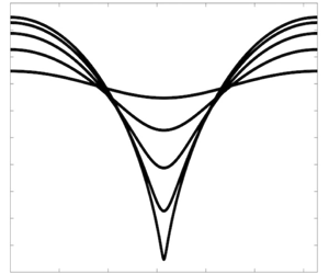
Equation (4.26) describes a particle trapped in a potential well, immediately yielding insightful qualitative information about the evolution of the amplitudes. Examples of potentials are shown in figure 2.

Figure 2.

Potential $\unicode[STIX]{x1D6F1}(\unicode[STIX]{x1D70C})$ when $\unicode[STIX]{x1D6EC}>0$ (black line) and $\unicode[STIX]{x1D6EC}<0$ (red line), where $\unicode[STIX]{x1D6EC}$ is defined in (4.28) and $\unicode[STIX]{x1D70C}=|\unicode[STIX]{x1D6FC}|$ . For the case of $\unicode[STIX]{x1D6EC}>0$ , the solutions are stable for all times. When $\unicode[STIX]{x1D6EC}<0$ , solutions may be unstable, leading to the formation of a cusp in the free surface as $\unicode[STIX]{x1D70C}\rightarrow 1/2$ .

For $\unicode[STIX]{x1D70C}$ small we see the potential goes to positive infinity, as ${\mathcal{P}}^{2}\geqslant 0$ . For $\unicode[STIX]{x1D70C}\rightarrow 1/2$ , the sign of the potential is given by the sign of

(4.28) $$\begin{eqnarray}\unicode[STIX]{x1D6EC}={\mathcal{P}}^{2}-H+1/8.\end{eqnarray}$$

When $\unicode[STIX]{x1D6EC}<0$ , solutions might lead to cusp formation as the value of $\unicode[STIX]{x1D70C}$ can approach $1/2$ .

5 Stokes waves

The normal mode linear stability of Stokes waves has been studied in detail by, for example, Longuet-Higgins (Reference Longuet-Higgins1978a ), McLean et al. (Reference McLean, Ma, Martin, Saffman and Yuen1981), Tanaka (Reference Tanaka1983) and MacKay & Saffman (Reference MacKay and Saffman1986). Here, we present an alternative derivation of the linear stability analysis with the added benefit that the system of equations takes a particularly simple form and is general. That is, once the Stokes coefficients (this may, for instance, be for class $M$ Stokes waves (Saffman Reference Saffman1980)) are determined, the stability analysis follows readily by solving an eigenvalue problem with prescribed matrix entries which are low-order polynomials in the dependent variables, making this approach particularly suitable for numerical implementation.

5.1 Stokes waves

We now consider permanent progressive solutions to the system where $N$ is taken to large enough to properly resolve the physical scenario in question.

To this end, we note that Stokes wave solutions to our system of equations take the simple form (Balk Reference Balk1996)

(5.1) $$\begin{eqnarray}Y_{k}=\unicode[STIX]{x1D6FC}_{k}\text{e}^{\text{i}ckt},\end{eqnarray}$$

so that $B_{k}=cY_{k}$ . The Lagrangian can then be written as

(5.2) $$\begin{eqnarray}L=-\frac{c^{2}Y_{0}}{2}+V,\end{eqnarray}$$

with $V$ given by equation (2.7). Therefore, the system governing the coefficients $\unicode[STIX]{x1D6FC}_{k}$ is (Longuet-Higgins (Reference Longuet-Higgins1985), see also Longuet-Higgins (Reference Longuet-Higgins1978c ))

(5.3) $$\begin{eqnarray}F_{n}=\unicode[STIX]{x1D6FC}_{n}(1+n\unicode[STIX]{x1D6FC}_{0})+\frac{1}{4}\sum (|n|+2|\,j|)\unicode[STIX]{x1D6FC}_{j}\unicode[STIX]{x1D6FC}_{k},\end{eqnarray}$$

for $F_{n}=0$ . There are $N+1$ equations here, so we must prescribe a parameter to close the system. Generally, the phase speed $c$ has been used. However, $c$ does not increase monotonically with increasing slope and contains critical points, which leads to loss in numerical accuracy (see § 5 of Longuet-Higgins (Reference Longuet-Higgins1985)). Alternatively, a variety of other parameters which do increase monotonically with increasing $ak$ have been proposed. Following Longuet-Higgins (Reference Longuet-Higgins1985), we take the parameter $Q=1-q_{crest}^{2}$ , where $q_{crest}$ is the particle speed at the crest. From Bernoulli’s equation, we have $Q=1+Y(0)=1+\frac{1}{2}\unicode[STIX]{x1D6FC}_{0}+\unicode[STIX]{x1D6FC}_{1}+\unicode[STIX]{x1D6FC}_{2}+\cdots \,.$ To solve the system of equations, i.e. (5.3), we employ a Newton–Raphson-type method.

5.2 Linear stability analysis

To find the form of the linear normal modes, we next let

(5.4) $$\begin{eqnarray}Y_{k}=(\unicode[STIX]{x1D6FC}_{k}+\unicode[STIX]{x1D716}A_{k}\text{e}^{\unicode[STIX]{x1D706}t})\text{e}^{\text{i}kct},\end{eqnarray}$$

where $\unicode[STIX]{x1D716}$ is a small parameter, $\unicode[STIX]{x1D706}$ is the normal mode eigenvalue and $A_{k}$ are the coefficients of the eigenvector.

The Lagrangian to $O(\unicode[STIX]{x1D716}^{2})$ becomes

(5.5) $$\begin{eqnarray}L=\frac{1}{2}\mathop{\sum }_{-N}^{N}|k|B_{k}B_{-k}+\frac{1}{2}Y_{0}^{2}-\mathop{\sum }_{1}^{N}Y_{k}Y_{-k}-\frac{1}{2}\mathop{\sum }_{j+k+l=0}^{\prime }|l|Y_{j}Y_{k}Y_{l},\end{eqnarray}$$

where

(5.6) $$\begin{eqnarray}B_{k}=\frac{\text{i}}{k}\left(-{\dot{Y}}_{k}-{\dot{Y}}_{0}Y_{k}|k|+\sum ^{\prime }{\dot{Y}}_{j}Y_{l}l(\unicode[STIX]{x1D70E}_{j}-\unicode[STIX]{x1D70E}_{l})\right),\end{eqnarray}$$

and primes represent sums over all indices except 0. Explicitly, the mean surface displacement is given by

(5.7) $$\begin{eqnarray}Y_{0}=-2\mathop{\sum }_{1}^{N}|k|\unicode[STIX]{x1D6FC}_{k}^{2}-\unicode[STIX]{x1D716}\mathop{\sum }_{-N}^{N}|k|\unicode[STIX]{x1D6FC}_{k}A_{-k}-\unicode[STIX]{x1D716}^{2}\mathop{\sum }_{-N}^{N}|k|A_{k}A_{-k},\end{eqnarray}$$

so that its time derivative is

(5.8) $$\begin{eqnarray}{\dot{Y}}_{0}=-\unicode[STIX]{x1D716}\mathop{\sum }_{-N}^{N}|k|\unicode[STIX]{x1D6FC}_{k}{\dot{A}}_{-k}-2\unicode[STIX]{x1D716}^{2}\mathop{\sum }_{-N}^{N}|k|{\dot{A}}_{k}A_{-k}.\end{eqnarray}$$

Substituting these relationships into the $B_{k}$ term, we find

(5.9) $$\begin{eqnarray}\displaystyle B_{k} & = & \displaystyle c\unicode[STIX]{x1D6FC}_{k}+\frac{\text{i}\unicode[STIX]{x1D716}}{k}\left(-({\dot{A}}_{k}+\text{i}ckA_{k})+\unicode[STIX]{x1D6FC}_{k}|k|\mathop{\sum }_{-N}^{N}|l|\unicode[STIX]{x1D6FC}_{l}{\dot{A}}_{-l}\right.\end{eqnarray}$$

(5.10) $$\begin{eqnarray}\displaystyle & & \displaystyle +\left.\sum [2\text{i}c(\unicode[STIX]{x1D6FC}_{j}A_{l}+\unicode[STIX]{x1D6FC}_{l}A_{j})+(\unicode[STIX]{x1D6FC}_{j}{\dot{A}}_{l}+\unicode[STIX]{x1D6FC}_{l}{\dot{A}}_{j})]\,jl(\unicode[STIX]{x1D70E}_{j}-\unicode[STIX]{x1D70E}_{l})\right)\end{eqnarray}$$

(5.11) $$\begin{eqnarray}\displaystyle & & \displaystyle +\,\frac{\text{i}\unicode[STIX]{x1D716}^{2}}{k}\left(-{\dot{Y}}_{0}^{(2)}|k|\unicode[STIX]{x1D6FC}_{k}-{\dot{Y}}_{0}^{(1)}|k|A_{k}+\sum ^{\prime }{\dot{A}}_{j}A_{l}l(\unicode[STIX]{x1D70E}_{j}-\unicode[STIX]{x1D70E}_{l})\right),\end{eqnarray}$$

where superscripts imply we are taking terms of that order from the expansion.

This is sufficient to define the Lagrangian. Applying the Euler–Lagrange equations, we find that the governing equation takes the form (cf. the discussion for the $N=1$ case in § 4) of a quadratic eigenvalue problem (Tisseur & Meerbergen Reference Tisseur and Meerbergen2001). Namely, we have

(5.12) $$\begin{eqnarray}(\unicode[STIX]{x1D706}^{2}\mathbb{M}+\unicode[STIX]{x1D706}\mathbb{C}+\mathbb{K})\boldsymbol{A}=\mathbf{0},\end{eqnarray}$$

where

(5.13) $$\begin{eqnarray}\unicode[STIX]{x1D6FE}_{n,m}=\frac{\text{i}}{n}\unicode[STIX]{x1D6FF}_{-n,m}+\frac{\text{i}}{n}\unicode[STIX]{x1D6FC}_{-n-m}(n+m)(\unicode[STIX]{x1D70E}_{m}-\unicode[STIX]{x1D70E}_{-n-m})-2\text{i}\unicode[STIX]{x1D70E}_{n}\unicode[STIX]{x1D6FC}_{n}|m|\unicode[STIX]{x1D6FC}_{m},\end{eqnarray}$$

for $\unicode[STIX]{x1D6FF}_{m,n}$ the Kronecker delta function, while

(5.14) $$\begin{eqnarray}\displaystyle \mathbb{M}_{n,m}=-\text{i}\unicode[STIX]{x1D70E}_{n}\unicode[STIX]{x1D6FE}_{n,m}+2\text{i}|n|\unicode[STIX]{x1D6FC}_{n}\left(\mathop{\sum }_{-N}^{N}l\unicode[STIX]{x1D6FC}_{l}\unicode[STIX]{x1D6FE}_{l,m}\right)+\text{i}\mathop{\sum }_{-N}^{N}\unicode[STIX]{x1D70E}_{l}\unicode[STIX]{x1D6FC}_{l-n}(l-n)\unicode[STIX]{x1D6FE}_{l,m}(\unicode[STIX]{x1D70E}_{n}-\unicode[STIX]{x1D70E}_{n-l}), & & \displaystyle\end{eqnarray}$$

(5.15) $$\begin{eqnarray}\displaystyle \mathbb{C}_{n,m} & = & \displaystyle 2\text{i}c\unicode[STIX]{x1D6FC}_{n+m}\unicode[STIX]{x1D70E}_{n+m}(\unicode[STIX]{x1D70E}_{m}-\unicode[STIX]{x1D70E}_{n})G(n,m)+2\text{i}cn|m|\unicode[STIX]{x1D6FC}_{n}\unicode[STIX]{x1D6FC}_{m}+c|n|\unicode[STIX]{x1D6FE}_{n,m}\nonumber\\ \displaystyle & & \displaystyle +\,\text{i}c\unicode[STIX]{x1D70E}_{n}\unicode[STIX]{x1D6FF}_{-n,m}+\text{i}c\unicode[STIX]{x1D70E}_{-m}(n+m)\unicode[STIX]{x1D6FC}_{n+m}(\unicode[STIX]{x1D70E}_{n}-\unicode[STIX]{x1D70E}_{-n-m})G(n,m),\end{eqnarray}$$

(5.16) $$\begin{eqnarray}\displaystyle \mathbb{K}_{n,m} & = & \displaystyle (1-c^{2}|n|)\unicode[STIX]{x1D6FF}_{-n,m}-4\left(\mathop{\sum }_{1}l\unicode[STIX]{x1D6FC}_{l}^{2}\right)|m|\unicode[STIX]{x1D6FF}_{n,-m}\nonumber\\ \displaystyle & & \displaystyle +\,-4|nm|\unicode[STIX]{x1D6FC}_{n}\unicode[STIX]{x1D6FC}_{m}+(|n|+|m|+G(n,m)|n+m|)\unicode[STIX]{x1D6FC}_{n+m},\end{eqnarray}$$

where $G(n,m)=1$ if $-N-m\leqslant n\leqslant N-m$ and 0 otherwise. The entries of these matrices are low-order polynomials in the Stokes coefficients, making them particularly suitable for numerical implementation. Furthermore, these results are general in the sense that one may examine subharmonic instabilities (Longuet-Higgins Reference Longuet-Higgins1978b ) by considering class $M$ , for $M$ a positive integer, Stokes waves (Saffman Reference Saffman1980; Zufiria Reference Zufiria1987).

To validate these algebraically complex computations, the eigenvalues corresponding to superharmonic perturbations of steep Stokes waves are computed from this method and are shown on top of the previous computations due to Tanaka (Reference Tanaka1983) in figure 3. Agreement between the predictions of equation (5.12) and Tanaka’s results are found. Furthermore, the change in (minus) total energy versus slope, $ak$ , is shown in the plot, showing that the change in stability corresponds to the critical point in the energy.

Figure 3.

A comparison of the eigenvalues squared of Tanaka (Reference Tanaka1983) (red dashed-dot line) versus the prediction given by Balk’s system, i.e. equation (5.12), shown by the black dots. The change in (minus) energy, $-E$ , with respect to $ak$ is shown by the blue dashed line.