


1. Motivation
The ARC $^{\textrm {TM}}$
Footnote
1
tokamak, designed to be a commercial fusion power plant (FPP), is part of a class of future machines that will operate as commercial power plants rather than flexible experimental devices. The manifestation of fusion-relevant plasmas at this scale will require robust operation to minimise the risk from plasma instabilities and disruptions, with more stringent limitations on diagnostics and control than on present research devices. For this reason, stable plasma scenarios must be designed and assessed prior to machine operation.
$^{\textrm {TM}}$
Footnote
1
tokamak, designed to be a commercial fusion power plant (FPP), is part of a class of future machines that will operate as commercial power plants rather than flexible experimental devices. The manifestation of fusion-relevant plasmas at this scale will require robust operation to minimise the risk from plasma instabilities and disruptions, with more stringent limitations on diagnostics and control than on present research devices. For this reason, stable plasma scenarios must be designed and assessed prior to machine operation.
In this paper, we discuss scenario and machine optimisation in ARC through the lens of magnetohydrodynamic (MHD) stability and control. In tokamaks, MHD stability can manifest itself through various critical phenomena, including the triggering of deleterious edge-Localised modes (ELMs) or global modes like the $n=0$
and
$n=0$
and $n=1$
modes, where
$n=1$
modes, where $n$
is the toroidal mode number of the instability. These instabilities place both hard and soft limits on the achievable plasma pressure normalised by the magnetic field pressure, known as the plasma beta (
$n$
is the toroidal mode number of the instability. These instabilities place both hard and soft limits on the achievable plasma pressure normalised by the magnetic field pressure, known as the plasma beta ( $\beta$
), and constrain the operational space available to any given machine.
$\beta$
), and constrain the operational space available to any given machine.
In order to assess the role that MHD stability will play in defining the accessible scenarios on the ARC tokamak, we utilise a series of well-validated physics codes to understand how changes in the ARC machine design will impact performance and control of the baseline power-producing scenario. As the design of ARC is still evolving, the following analyses are based on the ARC Version 3A and directly inform future iterations.
In § 2 the kinetic profiles and equilibrium as well as predicted rotation profiles used throughout this study are introduced. The first MHD stability investigated is the vertical stability control in § 3. Next, in § 4 the intrinsic three-dimensional (3-D) stability of the ARC baseline scenario is predicted. Specifically the ideal kink beta limit, linear tearing stability and neoclassical tearing modes are assessed. Lastly, in § 5 the critical $n=1$
error field causing locked modes and disruptions is predicted, and a physics basis to inform the design of error field correction coils (EFCCs) is formulated.
$n=1$
error field causing locked modes and disruptions is predicted, and a physics basis to inform the design of error field correction coils (EFCCs) is formulated.
2. The ARC kinetic equilibrium and profiles
For an as accurate as possible analysis of MHD physics a kinetic equilibrium is required in addition to estimated rotation profiles. This section describes how the kinetic profiles, rotation profiles and the kinetic equilibrium were informed and calculated. The starting point for this is a magnetic equilibrium generated by FreeGS (Dudson Reference Dudson2024) that was identified with cfsPOPCON (Body Reference Body2025) to meet the ARC target of approximately ${400}\,\textrm{MW}$
of net electricity with a fusion gain factor of
${400}\,\textrm{MW}$
of net electricity with a fusion gain factor of $Q = {50}{}$
. ARC uses an up–down symmetric double-null configuration with a triangularity of about
$Q = {50}{}$
. ARC uses an up–down symmetric double-null configuration with a triangularity of about $0.65$
and elongation of
$0.65$
and elongation of $1.8$
. More information on the process to generate this magnetic equilibrium is provided in Hillesheim et al. (Reference Hillesheim2026).
$1.8$
. More information on the process to generate this magnetic equilibrium is provided in Hillesheim et al. (Reference Hillesheim2026).
2.1. Kinetic profiles
The kinetic profiles are based on a combination of EPED (Snyder et al. Reference Snyder, Groebner, Leonard, Osborne and Wilson2009, Reference Snyder, Groebner, Hughes, Osborne, Beurskens, Leonard, Wilson and Xu2011) to set the H-mode pedestal width and height, and turbulent transport simulations to calculate the profiles in the core region. The core profiles used here are informed by ASTRA (Pereverzev & Yushmanov Reference Pereverzev and Yushmanov1991) coupled to the transport model TGLF (Staebler, Kinsey & Waltz Reference Staebler, Kinsey and Waltz2004) using saturation rule SAT2 (Staebler et al. Reference Staebler, Candy, Belli, Kinsey, Bonanomi and Patel2020). Furthermore, the separatrix temperature and density are informed by compatibility with detachment and operation in an ELM-free regime (Eich et al. Reference Eich2026). An overview of the transport simulation informing the ARC kinetic profiles as well as further high-fidelity simulations of core transport can be found in Howard et al. (Reference Howard2026).
The profiles of electron and main ion densities, temperatures and pressures are shown in figure 1 after slight smoothing and adding a boundary condition on the magnetic axis of vanishing derivatives. The main ions (50/50 deuterium and tritium) contribute to 85 % of the electron density across the entire radial range. The remaining electrons are the result of helium ash, hydrogen for ion cyclotron minority heating, tungsten and additional heavier impurities injected into the plasma to achieve the desired effective charge $Z_{\mathrm{eff}}$
. They are not further specified at this stage and a constant
$Z_{\mathrm{eff}}$
. They are not further specified at this stage and a constant $Z_{\mathrm{eff}}$
of 1.5 is assumed across the entire plasma.
$Z_{\mathrm{eff}}$
of 1.5 is assumed across the entire plasma.
Radial profiles of the electron and ion density (a), temperature (b) and pressure (c) as a function of the normalised poloidal flux. The dashed pressure line indicates the total pressure.

2.2. Kinetic equilibrium
The recently developed Grad–Shafranov solver TokaMaker (Hansen et al. Reference Hansen, Stewart, Burgess, Pharr, Guizzo, Logak, Nelson and Paz-Soldan2024) is used to calculate the Grad–Shafranov equilibrium which can be seen in figure 2(a). In order to reproduce the shape of the original FreeGS magnetic equilibrium the TokaMaker calculation is constrained by the two main x-points as well as a list of isoflux points that span the last closed flux surface (LCFS) of the original magnetic equilibrium all the way into the closed divertor. The high-field side (HFS) and low-field side (LFS) gaps between the wall and LCFS are set to approximately ${2}\,\mathrm{cm}$
. The kinetic profiles discussed in the previous section are used to constrain the pressure (b) and current profiles (c) including the bootstrap current
${2}\,\mathrm{cm}$
. The kinetic profiles discussed in the previous section are used to constrain the pressure (b) and current profiles (c) including the bootstrap current $j_{\mathrm{BS}}$
(Sauter, Angioni & Lin-Liu Reference Sauter, Angioni and Lin-Liu1999) over the whole radial range. ARC is designed to have a right-hand helicity with a negative plasma current
$j_{\mathrm{BS}}$
(Sauter, Angioni & Lin-Liu Reference Sauter, Angioni and Lin-Liu1999) over the whole radial range. ARC is designed to have a right-hand helicity with a negative plasma current $I_{\mathrm{p}}$
and negative toroidal magnetic field
$I_{\mathrm{p}}$
and negative toroidal magnetic field $B_{\mathrm{T}}$
pointing in the same toroidal direction. This results in a positive safety factor
$B_{\mathrm{T}}$
pointing in the same toroidal direction. This results in a positive safety factor $q$
profile, as seen in figure 2(b) with
$q$
profile, as seen in figure 2(b) with $q_{\mathrm{0}} \lt 1$
and
$q_{\mathrm{0}} \lt 1$
and $q_{\mathrm{95}} = 3.77$
. Rational surfaces used in the following studies are marked in figure 2(b) with vertical dashed lines in the core at
$q_{\mathrm{95}} = 3.77$
. Rational surfaces used in the following studies are marked in figure 2(b) with vertical dashed lines in the core at $q=1.5, 2.0, 2.5$
and in the edge near the pedestal top at
$q=1.5, 2.0, 2.5$
and in the edge near the pedestal top at $q=3.0, 3.33, 3.5$
.
$q=3.0, 3.33, 3.5$
.
(a) Poloidal cross-section of the kinetic equilibrium. (b) Total pressure and safety factor profile with relevant core and pedestal top rational surfaces indicated by vertical dashed lines with zoom-in in (c). (d) Current profiles and (e) radial electric field profiles from empirical extrapolations (blue) and a low rotation (green) and high rotation (red) case assuming a variation of 0.5× and 2.0× of the model results to cover the uncertainty bands. The vertical dashed line in (e) indicates the $q=2$
surface location which the empirical model was developed for.
$q=2$
surface location which the empirical model was developed for.

2.3. Rotation estimates
Because the workflows used in § 5 depend strongly on the $\boldsymbol{E}\times \boldsymbol{B}$
rotation with the electric field
$\boldsymbol{E}\times \boldsymbol{B}$
rotation with the electric field $\boldsymbol{E}$
and the magnetic field
$\boldsymbol{E}$
and the magnetic field $\boldsymbol{B}$
, predictions are made in the following to derive an
$\boldsymbol{B}$
, predictions are made in the following to derive an $\boldsymbol{E}\times \boldsymbol{B}$
rotation profile for ARC. Since ARC will use purely wave heating and no neutral beam injection, no substantial external torque input can be provided. Although substantial progress has been made over the last years in understanding the intrinsic torque and intrinsic plasma rotation, scalings and extrapolations are still uncertain and many contradicting scalings can be found (Rice et al. Reference Rice2007; Grierson et al. Reference Grierson, Burrell, Solomon, Budny and Candy2013; Chrystal et al. Reference Chrystal, Grierson, Haskey, Sontag, Poli, Shafer and deGrassie2020). Hence, the following extrapolations should be viewed with scepticism and we try to address this issue by including low and a high rotation cases to evaluate the impact of the highly uncertain rotation prediction.
$\boldsymbol{E}\times \boldsymbol{B}$
rotation profile for ARC. Since ARC will use purely wave heating and no neutral beam injection, no substantial external torque input can be provided. Although substantial progress has been made over the last years in understanding the intrinsic torque and intrinsic plasma rotation, scalings and extrapolations are still uncertain and many contradicting scalings can be found (Rice et al. Reference Rice2007; Grierson et al. Reference Grierson, Burrell, Solomon, Budny and Candy2013; Chrystal et al. Reference Chrystal, Grierson, Haskey, Sontag, Poli, Shafer and deGrassie2020). Hence, the following extrapolations should be viewed with scepticism and we try to address this issue by including low and a high rotation cases to evaluate the impact of the highly uncertain rotation prediction.
In order to estimate a radial electric field and consequent $\boldsymbol{E}\times \boldsymbol{B}$
rotation, we split the radial electric field
$\boldsymbol{E}\times \boldsymbol{B}$
rotation, we split the radial electric field $E_r$
profile up into a core and an edge part separated by a zero crossing assumed to be at a normalized poloidal flux of
$E_r$
profile up into a core and an edge part separated by a zero crossing assumed to be at a normalized poloidal flux of $\varPsi _{\mathrm{N}} = 0.93$
which is close to the pedestal top. Furthermore we assume a vanishing radial electric field at the separatrix. In the core, the radial electric field is defined mostly by the contribution from the toroidal rotation, which is estimated based on an empirical scaling developed in Rice et al. (Reference Rice2007) for purely wave-heated plasmas including multiple tokamaks of varying size. In particular, the toroidal rotation measured on the
$\varPsi _{\mathrm{N}} = 0.93$
which is close to the pedestal top. Furthermore we assume a vanishing radial electric field at the separatrix. In the core, the radial electric field is defined mostly by the contribution from the toroidal rotation, which is estimated based on an empirical scaling developed in Rice et al. (Reference Rice2007) for purely wave-heated plasmas including multiple tokamaks of varying size. In particular, the toroidal rotation measured on the $q=2$
surface normalised to the Alfvén velocity, that is the Alfvén Mach number
$q=2$
surface normalised to the Alfvén velocity, that is the Alfvén Mach number $M_{\mathrm{A}}$
, was identified to scale well with the toroidal beta
$M_{\mathrm{A}}$
, was identified to scale well with the toroidal beta $\beta _{\mathrm{t}}$
and the cylindrical safety factor
$\beta _{\mathrm{t}}$
and the cylindrical safety factor $q^*$
as
$q^*$
as $M_{\mathrm{A}} = 0.65 \beta _{\mathrm{T}}^{1.4}q^{*2.3}$
. While this scaling was only developed for the rotation at the
$M_{\mathrm{A}} = 0.65 \beta _{\mathrm{T}}^{1.4}q^{*2.3}$
. While this scaling was only developed for the rotation at the $q=2$
surface, the codes used in this work require complete radial profiles. Therefore it is assumed that it is a reasonable approximation in the whole core region ranging from
$q=2$
surface, the codes used in this work require complete radial profiles. Therefore it is assumed that it is a reasonable approximation in the whole core region ranging from $\varPsi _{\mathrm{N}} = 0.0$
to
$\varPsi _{\mathrm{N}} = 0.0$
to $\varPsi _{\mathrm{q=2}} + 0.05$
. In the edge, the radial electric field in an H-mode plasma typically forms a so-called
$\varPsi _{\mathrm{q=2}} + 0.05$
. In the edge, the radial electric field in an H-mode plasma typically forms a so-called $E_{\mathrm{r}}$
well. Due to the steep gradients at this location, for the main ions species the diamagnetic term in the radial ion force balance is dominant and can be used as an approximation for the
$E_{\mathrm{r}}$
well. Due to the steep gradients at this location, for the main ions species the diamagnetic term in the radial ion force balance is dominant and can be used as an approximation for the $E_{\mathrm{r}}$
well (Viezzer et al. Reference Viezzer, Pütterich, Angioni, Bergmann, Dux, Fable, McDermott, Stroth and Wolfrum2013). Combining the
$E_{\mathrm{r}}$
well (Viezzer et al. Reference Viezzer, Pütterich, Angioni, Bergmann, Dux, Fable, McDermott, Stroth and Wolfrum2013). Combining the $E_{\mathrm{r}}$
estimates in the core and edge results in the radial electric field profiles as shown in figure 2(e) for the three different cases: the model prediction (blue), a high rotation case with 2x the intrinsic rotation prediction (red) and a low rotation case with a multiplier of 0.5 (green). This captures the uncertainty of the model well.
$E_{\mathrm{r}}$
estimates in the core and edge results in the radial electric field profiles as shown in figure 2(e) for the three different cases: the model prediction (blue), a high rotation case with 2x the intrinsic rotation prediction (red) and a low rotation case with a multiplier of 0.5 (green). This captures the uncertainty of the model well.
Furthermore, a simple model for error field correction introduced later in Appendix A requires the intrinsic torque of the plasma. The intrinsic torque for ARC V0 is also predicted in Rice et al. (Reference Rice, Cao, Tala, Chrystal, Greenwald, Hughes, Marmar, Reinke, Fernandez and Salmi2021) as $T_{\mathrm{0}} = {8}\,\,\mathrm{Nm}$
. Considering the uncertainties in this model and the current ARC V3A design, using the scaling law a reasonable intrinsic torque would be in the range of
$T_{\mathrm{0}} = {8}\,\,\mathrm{Nm}$
. Considering the uncertainties in this model and the current ARC V3A design, using the scaling law a reasonable intrinsic torque would be in the range of $5$
–
$5$
– ${20}\,\mathrm{Nm}$
.
${20}\,\mathrm{Nm}$
.
Currently, rotation modelling lacks a precise boundary condition in the plasma edge, as the underlying physical processes are still under discussion. Therefore, to map out the effects of various models, a second workflow is applied using an alternative approach. Within the plasma core, turbulent momentum transport governs the formation of the rotation profile in the absence of strong transient events. Under these conditions, the workflow presented in Zimmermann et al. (Reference Zimmermann2024), which incorporates semi-empirical and validated turbulent momentum transport models, can be applied. For this purpose, it is conservative to assume zero edge rotation, for example, at the pedestal top. A dimensionless, normalised version of this model yields an intrinsic torque of approximately ${30}\,\mathrm{Nm}$
at the
${30}\,\mathrm{Nm}$
at the $q=2$
surface. It exceeds even the optimistic prediction from Rice et al. (Reference Rice, Cao, Tala, Chrystal, Greenwald, Hughes, Marmar, Reinke, Fernandez and Salmi2021) by a factor of 1.5. This intrinsic torque leads only to moderate toroidal rotation values due to the correspondingly large plasma mass. With a predicted
$q=2$
surface. It exceeds even the optimistic prediction from Rice et al. (Reference Rice, Cao, Tala, Chrystal, Greenwald, Hughes, Marmar, Reinke, Fernandez and Salmi2021) by a factor of 1.5. This intrinsic torque leads only to moderate toroidal rotation values due to the correspondingly large plasma mass. With a predicted ${3}{}$
–
${3}{}$
– ${9}\,\mathrm{krad\,s}^{-1}$
it predicts values similar to the pessimistic case, and one finds slightly lower rotation values at
${9}\,\mathrm{krad\,s}^{-1}$
it predicts values similar to the pessimistic case, and one finds slightly lower rotation values at $q = 2$
than those predicted by the scaling in Rice et al. (Reference Rice2007). This comparison confirms that a choice of a low rotation case with the low toroidal rotation of 0.5× the model prediction and
$q = 2$
than those predicted by the scaling in Rice et al. (Reference Rice2007). This comparison confirms that a choice of a low rotation case with the low toroidal rotation of 0.5× the model prediction and $T_{\mathrm{0}}={5}\,\mathrm{Nm}$
, a mid rotation case with the model prediction for the toroidal rotation and
$T_{\mathrm{0}}={5}\,\mathrm{Nm}$
, a mid rotation case with the model prediction for the toroidal rotation and $T_{\mathrm{0}}={10}\,\mathrm{Nm}$
and a high rotation case with the high toroidal rotation of 2.0x the model prediction and
$T_{\mathrm{0}}={10}\,\mathrm{Nm}$
and a high rotation case with the high toroidal rotation of 2.0x the model prediction and $T_{\mathrm{0}}={20}\,\mathrm{Nm}$
provides good coverage of possible rotation profiles.
$T_{\mathrm{0}}={20}\,\mathrm{Nm}$
provides good coverage of possible rotation profiles.
3. Vertical stability of the ARC baseline scenario
Vertical stability, or control of the $n=0$
resistive wall mode, is a fundamental issue for tokamak designs as it both limits the maximum achievable elongation in a particular scenario and constrains the engineering of superconducting poloidal field (PF) coil sets and their respective power supplies. In order to assess the feasibility of vertical control for the ARC machine, a series of iterative studies are performed with the MEQ-FGE/FGS/FBT (Carpanese Reference Carpanese2021) and TokaMaker (Hansen et al. Reference Hansen, Stewart, Burgess, Pharr, Guizzo, Logak, Nelson and Paz-Soldan2024) codes, following the generalised procedures outlined in previous work for the SPARC device (Nelson et al. Reference Nelson, Garnier, Battaglia, Paz-Soldan, Stewart, Reinke, Creely and Wai2024). Importantly, the vertical control capabilities of ARC both need to function under the power supply requirements associated with active superconducting coils and be able to demonstrate robustness against the large eddy currents that will develop in the thick conducting ARC vacuum vessel and structures. The conducting elements of the ARC vessel and the associated
$n=0$
resistive wall mode, is a fundamental issue for tokamak designs as it both limits the maximum achievable elongation in a particular scenario and constrains the engineering of superconducting poloidal field (PF) coil sets and their respective power supplies. In order to assess the feasibility of vertical control for the ARC machine, a series of iterative studies are performed with the MEQ-FGE/FGS/FBT (Carpanese Reference Carpanese2021) and TokaMaker (Hansen et al. Reference Hansen, Stewart, Burgess, Pharr, Guizzo, Logak, Nelson and Paz-Soldan2024) codes, following the generalised procedures outlined in previous work for the SPARC device (Nelson et al. Reference Nelson, Garnier, Battaglia, Paz-Soldan, Stewart, Reinke, Creely and Wai2024). Importantly, the vertical control capabilities of ARC both need to function under the power supply requirements associated with active superconducting coils and be able to demonstrate robustness against the large eddy currents that will develop in the thick conducting ARC vacuum vessel and structures. The conducting elements of the ARC vessel and the associated $L/R$
time with inductance
$L/R$
time with inductance $L$
and resistance
$L$
and resistance $R$
are also important for studies of disruption mitigation, as discussed in Sweeney et al. (Reference Sweeney2026). Both codes employed here are capable of solving the integrated temporal dynamics of conductor current evolution and resistive plasma current decay, allowing for accurate assessments of the plasma and machine state during the rapid motion expected during a vertical displacement event. For details on the formulation of these calculations, the reader is directed to expanded discussions in Carpanese (Reference Carpanese2021), Hansen et al. (Reference Hansen, Stewart, Burgess, Pharr, Guizzo, Logak, Nelson and Paz-Soldan2024), Nelson et al. (Reference Nelson, Garnier, Battaglia, Paz-Soldan, Stewart, Reinke, Creely and Wai2024), Guizzo et al. (Reference Guizzo, Nelson, Hansen, Logak and Paz-Soldan2024) and Kumar et al. (Reference Kumar, Clauser, Carpanese, Wai, Golfinopoulos, Battaglia, Garnier, Granetz, Sweeney and Boyer2026). For all calculations presented here, good agreement is observed between the TokaMaker and MEQ-FGE models. Critically, to further increase confidence in the ARC design, both models will be validated upon SPARC data when they become available.
$R$
are also important for studies of disruption mitigation, as discussed in Sweeney et al. (Reference Sweeney2026). Both codes employed here are capable of solving the integrated temporal dynamics of conductor current evolution and resistive plasma current decay, allowing for accurate assessments of the plasma and machine state during the rapid motion expected during a vertical displacement event. For details on the formulation of these calculations, the reader is directed to expanded discussions in Carpanese (Reference Carpanese2021), Hansen et al. (Reference Hansen, Stewart, Burgess, Pharr, Guizzo, Logak, Nelson and Paz-Soldan2024), Nelson et al. (Reference Nelson, Garnier, Battaglia, Paz-Soldan, Stewart, Reinke, Creely and Wai2024), Guizzo et al. (Reference Guizzo, Nelson, Hansen, Logak and Paz-Soldan2024) and Kumar et al. (Reference Kumar, Clauser, Carpanese, Wai, Golfinopoulos, Battaglia, Garnier, Granetz, Sweeney and Boyer2026). For all calculations presented here, good agreement is observed between the TokaMaker and MEQ-FGE models. Critically, to further increase confidence in the ARC design, both models will be validated upon SPARC data when they become available.
(a) The separatrix of an example ARC equilibrium evolving through an initial ${10}\,\mathrm{cm}$
vertical displacement towards nominal conditions under vertical control with the PF5 coil (red), as modelled with the TokaMaker code. For a scan of varying initial displacements, the magnetic axis location (b), the current used for vertical control (c) and the power supply voltage needed to create this current (d) are also plotted.
${10}\,\mathrm{cm}$
vertical displacement towards nominal conditions under vertical control with the PF5 coil (red), as modelled with the TokaMaker code. For a scan of varying initial displacements, the magnetic axis location (b), the current used for vertical control (c) and the power supply voltage needed to create this current (d) are also plotted.

One of the key performance metrics for a vertical control system is maximum controllable displacement $\varDelta Z_{\mathrm{max}}$
, which characterises the robustness of a vertical control system to spontaneous vertical excursions that may arise from measurement noise, internal MHD events, rapid changes in the plasma current distribution or ELMs (Humphreys et al. Reference Humphreys2009; Nelson et al. Reference Nelson, Garnier, Battaglia, Paz-Soldan, Stewart, Reinke, Creely and Wai2024). In general, the ability to control displacements of the order of
$\varDelta Z_{\mathrm{max}}$
, which characterises the robustness of a vertical control system to spontaneous vertical excursions that may arise from measurement noise, internal MHD events, rapid changes in the plasma current distribution or ELMs (Humphreys et al. Reference Humphreys2009; Nelson et al. Reference Nelson, Garnier, Battaglia, Paz-Soldan, Stewart, Reinke, Creely and Wai2024). In general, the ability to control displacements of the order of $\varDelta Z_{\mathrm{max}}/a_{\mathrm{minor}}\sim 5\,\%$
, where
$\varDelta Z_{\mathrm{max}}/a_{\mathrm{minor}}\sim 5\,\%$
, where $a_{\mathrm{minor}}$
is the minor radius of the plasma, corresponds to ‘safe’ operation in which a tolerable number of vertical excursions are stabilised before leading to a full disruption. As such, the ARC, SPARC, ITER and DEMO designs all target that their control systems be able to, at a minimum, stabilise vertical excursions with initial displacements of
$a_{\mathrm{minor}}$
is the minor radius of the plasma, corresponds to ‘safe’ operation in which a tolerable number of vertical excursions are stabilised before leading to a full disruption. As such, the ARC, SPARC, ITER and DEMO designs all target that their control systems be able to, at a minimum, stabilise vertical excursions with initial displacements of $\varDelta Z_{\mathrm{max}}/a_{\mathrm{minor}}\gtrsim 5\,\%$
(Humphreys et al. Reference Humphreys2009; Villone et al. Reference Villone, Barbato, Mastrostefano and Ventre2013; Hahn et al. Reference Hahn2020; Nelson et al. Reference Nelson, Hyatt, Wehner, Welander, Paz-Soldan, Osborne, Anand and Thome2023; Nelson et al. Reference Nelson, Garnier, Battaglia, Paz-Soldan, Stewart, Reinke, Creely and Wai2024). On ARC, this suggests that the vertical stability system must be able to tolerate displacements of at least
$\varDelta Z_{\mathrm{max}}/a_{\mathrm{minor}}\gtrsim 5\,\%$
(Humphreys et al. Reference Humphreys2009; Villone et al. Reference Villone, Barbato, Mastrostefano and Ventre2013; Hahn et al. Reference Hahn2020; Nelson et al. Reference Nelson, Hyatt, Wehner, Welander, Paz-Soldan, Osborne, Anand and Thome2023; Nelson et al. Reference Nelson, Garnier, Battaglia, Paz-Soldan, Stewart, Reinke, Creely and Wai2024). On ARC, this suggests that the vertical stability system must be able to tolerate displacements of at least $\varDelta Z_{\mathrm{max}} \sim 6$
cm for safe operation.
$\varDelta Z_{\mathrm{max}} \sim 6$
cm for safe operation.
To evaluate $\varDelta Z_{\mathrm{max}}$
for ARC, equilibria subject to a minimum initial displacement are allowed to evolve in both TokaMaker and MEQ-FGE subject to applied control schemes and self-consistent vessel and eddy currents. An example of this evolution is shown in figure 3(a) for a representative ARC equilibrium. Due to the hostile environment in a high fusion power tokamak, ARC will utilise its poloidal shaping coils for vertical stability control instead of dedicated in-vessel coils. Only the upper and lower PF5 coils (shown in red) are used here to enforce the vertical stability circuit in a split-control configuration. As both TokaMaker and MEQ-FGE allow for explicit design of the target machine, scans of elongation and variations in the ARC shaping coil locations were conducted in parallel to other performance and engineering design tasks. For each iteration of the ARC design, calculations of
$\varDelta Z_{\mathrm{max}}$
for ARC, equilibria subject to a minimum initial displacement are allowed to evolve in both TokaMaker and MEQ-FGE subject to applied control schemes and self-consistent vessel and eddy currents. An example of this evolution is shown in figure 3(a) for a representative ARC equilibrium. Due to the hostile environment in a high fusion power tokamak, ARC will utilise its poloidal shaping coils for vertical stability control instead of dedicated in-vessel coils. Only the upper and lower PF5 coils (shown in red) are used here to enforce the vertical stability circuit in a split-control configuration. As both TokaMaker and MEQ-FGE allow for explicit design of the target machine, scans of elongation and variations in the ARC shaping coil locations were conducted in parallel to other performance and engineering design tasks. For each iteration of the ARC design, calculations of $\varDelta Z_{\mathrm{max}}$
were extracted from scans of
$\varDelta Z_{\mathrm{max}}$
were extracted from scans of $\varDelta Z_{\mathrm{0}}$
, as shown in figure 3(b), to inform design decisions such as the target elongation. As an illustration of this process, figures 3(c) and 3(d) show the current (
$\varDelta Z_{\mathrm{0}}$
, as shown in figure 3(b), to inform design decisions such as the target elongation. As an illustration of this process, figures 3(c) and 3(d) show the current ( $I_{\mathrm{VS}}$
) and voltage (
$I_{\mathrm{VS}}$
) and voltage ( $V_{\mathrm{VS}}$
) of the vertical stability circuit, respectively, for a particular set of engineering constraints, which may continue to evolve as ARC is constructed. The presented simulation is conducted with an assumption of 100 turns per PF coil, similar to the coil designs of the SPARC tokamak (Nelson et al. Reference Nelson, Garnier, Battaglia, Paz-Soldan, Stewart, Reinke, Creely and Wai2024). This assumption, which impacts the coil self-inductance and required voltage but will not likely substantially change the vertical controllability of ARC plasmas, is expected to change as the power supply systems for ARC are refined. In addition, future iterations of the ARC design may include additional passive stabilising elements to alleviate the burden of vertical stability control on the power supplies. In the simulation shown in figure 3, which includes a
$V_{\mathrm{VS}}$
) of the vertical stability circuit, respectively, for a particular set of engineering constraints, which may continue to evolve as ARC is constructed. The presented simulation is conducted with an assumption of 100 turns per PF coil, similar to the coil designs of the SPARC tokamak (Nelson et al. Reference Nelson, Garnier, Battaglia, Paz-Soldan, Stewart, Reinke, Creely and Wai2024). This assumption, which impacts the coil self-inductance and required voltage but will not likely substantially change the vertical controllability of ARC plasmas, is expected to change as the power supply systems for ARC are refined. In addition, future iterations of the ARC design may include additional passive stabilising elements to alleviate the burden of vertical stability control on the power supplies. In the simulation shown in figure 3, which includes a ${100}\,\mathrm{ms}$
delay in the control system and a maximum rate of change of
${100}\,\mathrm{ms}$
delay in the control system and a maximum rate of change of ${200}\,\mathrm{kV}\,\mathrm{s}^{-1}$
for the vertical stability power supplies, the
${200}\,\mathrm{kV}\,\mathrm{s}^{-1}$
for the vertical stability power supplies, the $I_{\mathrm{VS}}$
slew rate limit of
$I_{\mathrm{VS}}$
slew rate limit of ${2.5}\,\mathrm{kA}\,(\mathrm{ms})^{-1}$
becomes the limiting parameter for vertical stability control. Using these parameters,
${2.5}\,\mathrm{kA}\,(\mathrm{ms})^{-1}$
becomes the limiting parameter for vertical stability control. Using these parameters, $\varDelta Z_{\mathrm{max}}\sim {12}\,\mathrm{cm}$
is achieved for the ARC baseline scenario, which is approximately twice the expected margin needed for safe operation.
$\varDelta Z_{\mathrm{max}}\sim {12}\,\mathrm{cm}$
is achieved for the ARC baseline scenario, which is approximately twice the expected margin needed for safe operation.
In addition to large scale changes to equilibrium and machine conditions, several potential design trade-offs associated with vertical stability modelling result from specifics of the power supplies that control the coils used for vertical stability control. In particular, variations in the voltage and current slew rates, limits in the maximum power supply voltage and the time delay of filters and diagnostics can all significantly impact the controllability of ARC plasmas. To illustrate this point, sensitivity scans of the voltage slew rate limit and the vertical control filter time are presented in figure 4 for cases where the PF5s are voltage limited, as opposed to the current-limited case presented in figure 3. The requirement that $\varDelta Z_{\mathrm{max}}/a_{\mathrm{minor}}\gt 5\,\%$
be maintained for safe machine operation places direct demands on the engineering parameters associated with the power supplies. Predictions of
$\varDelta Z_{\mathrm{max}}/a_{\mathrm{minor}}\gt 5\,\%$
be maintained for safe machine operation places direct demands on the engineering parameters associated with the power supplies. Predictions of $\varDelta Z_{\max}$
are also sensitive to the number of turns of each PF coil, which was also scanned in this work but remains a free parameter in the present ARC design that will ultimately be set by magnet and power supply design. The precise behaviour of the vertical stability system is expected to change as this value is updated in future iterations of the ARC machine: more turns will reduce the
$\varDelta Z_{\max}$
are also sensitive to the number of turns of each PF coil, which was also scanned in this work but remains a free parameter in the present ARC design that will ultimately be set by magnet and power supply design. The precise behaviour of the vertical stability system is expected to change as this value is updated in future iterations of the ARC machine: more turns will reduce the $I_{\mathrm{VS}}$
per turn needed for stabilisation but increase the effective inductance and required power supply voltage.
$I_{\mathrm{VS}}$
per turn needed for stabilisation but increase the effective inductance and required power supply voltage.
The maximum controllable displacement for the ARC baseline design for various filter delay times and voltage slew rates calculated with the MEQ-FGE code. The requirement of $\varDelta Z_{max}/a_{minor}\gt 5\,\%$
where
$\varDelta Z_{max}/a_{minor}\gt 5\,\%$
where $a_{minor}={1.18}\,\mathrm{m}$
sets engineering limits for power supplies and current systems in ARC.
$a_{minor}={1.18}\,\mathrm{m}$
sets engineering limits for power supplies and current systems in ARC.

This design of the ARC tokamak also features a liquid immersion blanket with the molten salt FLiBe, which provides cooling to the vacuum vessel, functions both as a tritium breeding medium and a neutron multiplier, and provides neutron shielding to the coils (Hillesheim et al. Reference Hillesheim2026). While the FLiBe blanket provides many benefits for the ARC design, it also introduces another source of uncertainty into machine modelling as the fusion community is still relatively inexperienced in working with the material. To assess the potential impact of a thick FLiBe layer throughout the blanket region, an additional conducting layer with a conductivity of 200 Sm−1, which is estimated to be appropriate for FLiBe at 600 $^\circ$
C based on (Janz Reference Janz1988), was added to the ARC design in TokaMaker. Since other machine elements are orders of magnitude more conducting, the addition of the FLiBe blanket is found to have little effect on the growth or control of vertical instabilities in ARC. Any induced motion in the FLiBe, while expected to be small compared with the timescale of the magnetic field changes, is ignored in this analysis.
$^\circ$
C based on (Janz Reference Janz1988), was added to the ARC design in TokaMaker. Since other machine elements are orders of magnitude more conducting, the addition of the FLiBe blanket is found to have little effect on the growth or control of vertical instabilities in ARC. Any induced motion in the FLiBe, while expected to be small compared with the timescale of the magnetic field changes, is ignored in this analysis.
While the precise determination of parameters associated with the vertical stability control system are still being finalised, the scans presented here highlight the impact that predictive vertical stability modelling can have on critical design decisions. Notably, the above results demonstrate that ARC plasmas should be controllable without a dedicated vertical stability coil inside of the vacuum vessel, which could otherwise be complicated to design, install and maintain.
4. Intrinsic 3-D stability
The thermal pressure of every tokamak plasma is ultimately limited by the magnetic pressure of the magnetic field confining the plasma. In practice, this limit can never be reached due to plasma instabilities such as kink and ballooning modes that already become unstable at a much lower thermal pressure or plasma beta, which scales roughly with $I_{\mathrm{p}} / (a_{\mathrm{minor}} \boldsymbol{\cdot }B_{\mathrm{T}})$
. This motivates the definition of the normalised plasma beta as
$I_{\mathrm{p}} / (a_{\mathrm{minor}} \boldsymbol{\cdot }B_{\mathrm{T}})$
. This motivates the definition of the normalised plasma beta as $\beta _{\mathrm{N}} = {\beta }/({I_{\mathrm{p}} / (a_{\mathrm{minor}} \boldsymbol{\cdot }B_{\mathrm{T}})})$
. In a conventional (non-spherical) tokamak the maximum achievable
$\beta _{\mathrm{N}} = {\beta }/({I_{\mathrm{p}} / (a_{\mathrm{minor}} \boldsymbol{\cdot }B_{\mathrm{T}})})$
. In a conventional (non-spherical) tokamak the maximum achievable $\beta _{\mathrm{N}}$
is in the range of roughly
$\beta _{\mathrm{N}}$
is in the range of roughly $3{-}6$
(Strait Reference Strait2005), which is generally considered sufficient for a power plant design. However, resistive MHD instabilities such as neoclassical tearing modes can lead to an even lower soft
$3{-}6$
(Strait Reference Strait2005), which is generally considered sufficient for a power plant design. However, resistive MHD instabilities such as neoclassical tearing modes can lead to an even lower soft $\beta$
limit. In this section we investigate the ideal beta limit in § 4.1, which is the
$\beta$
limit. In this section we investigate the ideal beta limit in § 4.1, which is the $\beta _{\mathrm{N}}$
at which ideal kink or ballooning modes become unstable, as well as ideal and resistive stability of classical and neoclassical tearing modes in § 4.2.
$\beta _{\mathrm{N}}$
at which ideal kink or ballooning modes become unstable, as well as ideal and resistive stability of classical and neoclassical tearing modes in § 4.2.
4.1. Ideal kink pressure limit
The Direct Criterion of Newcomb (DCON) code (Glasser Reference Glasser2016) uses the formalism described in Newcomb (Reference Newcomb1960) to calculate the ideal MHD kink stability of a plasma for toroidal axisymmetric geometry. As a metric for stability, DCON calculates the total energy matrix $W_{\mathrm{T}}$
including the plasma response. If
$W_{\mathrm{T}}$
including the plasma response. If $W_{\mathrm{T}}$
has any negative eigenvalues, then an external mode is unstable. We use this criterion to assess the beta limit for ideal MHD stability of an ARC plasma for
$W_{\mathrm{T}}$
has any negative eigenvalues, then an external mode is unstable. We use this criterion to assess the beta limit for ideal MHD stability of an ARC plasma for $n=1$
.
$n=1$
.
In order to assess the beta limit, the original ARC equilibrium with $\beta _{\mathrm{N}} = 1.65$
is evaluated as well as a set of equilibria that are generated with TokaMaker by scaling the pressure profile up or down and solving the free-boundary equilibrium with self-consistent bootstrap current. Figure 5(a) shows the minimum eigenvalue of the
$\beta _{\mathrm{N}} = 1.65$
is evaluated as well as a set of equilibria that are generated with TokaMaker by scaling the pressure profile up or down and solving the free-boundary equilibrium with self-consistent bootstrap current. Figure 5(a) shows the minimum eigenvalue of the $W_{\mathrm{T}}$
matrix as a function of
$W_{\mathrm{T}}$
matrix as a function of $\beta _{\mathrm{N}}$
for three different cases. The blue dots represent the case without a conducting wall and without kinetic effects. The minimum
$\beta _{\mathrm{N}}$
for three different cases. The blue dots represent the case without a conducting wall and without kinetic effects. The minimum $W_{\mathrm{T}}$
eigenvalues become negative, i.e. the ideal beta limit is reached, at
$W_{\mathrm{T}}$
eigenvalues become negative, i.e. the ideal beta limit is reached, at $\beta _{\mathrm{N}} \approx 3.2$
which is roughly a factor of
$\beta _{\mathrm{N}} \approx 3.2$
which is roughly a factor of $2$
above the nominal value. Hence, we conclude that the ARC plasma is stable and operates at a safe distance from the ideal beta limit. Including a conducting wall can lead to a passive stabilisation of the plasma due to eddy currents in the wall. The DCON code generates a conducting wall with the same shape as the LCFS at a given distance, which we assumed such as to have the conducting wall just behind the first wall of ARC as shown in figure 5(b). As expected, the eigenvalue minima are higher in the wall case (green dots) than in the no-wall case (blue dots) meaning that the plasma is even more stable. Including kinetic damping effects (Logan et al. Reference Logan, Park, Kim, Wang and Berkery2013; Park & Logan Reference Park and Logan2017) in addition to the conducting wall (red crosses) has only a negligible effect, of the order of 1 %.
$2$
above the nominal value. Hence, we conclude that the ARC plasma is stable and operates at a safe distance from the ideal beta limit. Including a conducting wall can lead to a passive stabilisation of the plasma due to eddy currents in the wall. The DCON code generates a conducting wall with the same shape as the LCFS at a given distance, which we assumed such as to have the conducting wall just behind the first wall of ARC as shown in figure 5(b). As expected, the eigenvalue minima are higher in the wall case (green dots) than in the no-wall case (blue dots) meaning that the plasma is even more stable. Including kinetic damping effects (Logan et al. Reference Logan, Park, Kim, Wang and Berkery2013; Park & Logan Reference Park and Logan2017) in addition to the conducting wall (red crosses) has only a negligible effect, of the order of 1 %.
In conclusion, even when assuming the most unstable case without the stabilisation from a conducting wall or kinetic effects, the plasma is still predicted to be far away from the ideal kink beta limit for ARC.
(a) The minimum of the total response matrix $W_{\mathrm{T}}$
eigenvalues as a function of the normalised beta
$W_{\mathrm{T}}$
eigenvalues as a function of the normalised beta $\beta _{\mathrm{N}}$
. Three different cases are shown, the no-wall limit (blue), including a conducting wall (green) and including a conducting wall as well as kinetic effects (red). The vertical dashed black line indicates the
$\beta _{\mathrm{N}}$
. Three different cases are shown, the no-wall limit (blue), including a conducting wall (green) and including a conducting wall as well as kinetic effects (red). The vertical dashed black line indicates the $\beta _{\mathrm{N}}$
of the nominal ARC V3A equilibrium. (b) Poloidal cross-section showing the separatrix (red), the first wall (green) and the location of the conducting wall as used in DCON (blue).
$\beta _{\mathrm{N}}$
of the nominal ARC V3A equilibrium. (b) Poloidal cross-section showing the separatrix (red), the first wall (green) and the location of the conducting wall as used in DCON (blue).

4.2. Tearing stability
Tearing modes are deleterious resistive MHD instabilities that grow on rational ( $q=m/n$
for poloidal and toroidal mode numbers
$q=m/n$
for poloidal and toroidal mode numbers $m$
and
$m$
and $n$
) surfaces, breaking nested flux surfaces into periodic magnetic islands that can reduce confinement and lead to disruptions. Once grown to sufficient size, tearing modes can induce eddy currents in the device wall that brake their toroidal rotation and drag on the plasma, potentially leading to mode locking and disruption (de Vries et al. Reference de Vries, Johnson, Alper, Buratti, Hender, Koslowski, Riccardo and Contributors2011; Sweeney et al. Reference Sweeney, Choi, La Haye, Mao, Olofsson and Volpe2017). In § 4.2.1 we calculate using STRIDE (Glasser & Kolemen Reference Glasser and Kolemen2018) and an analytic proxy for Glasser stabilisation (Glasser et al. Reference Glasser, Greene and Johnson1975; Lütjens et al. Reference Lütjens, Luciani and Garbet2001) that ARC is robustly linearly stable to tearing modes, a necessary hurdle for any tokamak fusion plant. In § 4.2.2 we evaluate the nonlinear tearing stability of ARC in the context of other hypothetical plasma scenarios, using a modified Rutherford equation analysis (Rutherford Reference Rutherford1973; Hegna Reference Hegna1999; Schlutt & Hegna Reference Schlutt and Hegna2012).
$n$
) surfaces, breaking nested flux surfaces into periodic magnetic islands that can reduce confinement and lead to disruptions. Once grown to sufficient size, tearing modes can induce eddy currents in the device wall that brake their toroidal rotation and drag on the plasma, potentially leading to mode locking and disruption (de Vries et al. Reference de Vries, Johnson, Alper, Buratti, Hender, Koslowski, Riccardo and Contributors2011; Sweeney et al. Reference Sweeney, Choi, La Haye, Mao, Olofsson and Volpe2017). In § 4.2.1 we calculate using STRIDE (Glasser & Kolemen Reference Glasser and Kolemen2018) and an analytic proxy for Glasser stabilisation (Glasser et al. Reference Glasser, Greene and Johnson1975; Lütjens et al. Reference Lütjens, Luciani and Garbet2001) that ARC is robustly linearly stable to tearing modes, a necessary hurdle for any tokamak fusion plant. In § 4.2.2 we evaluate the nonlinear tearing stability of ARC in the context of other hypothetical plasma scenarios, using a modified Rutherford equation analysis (Rutherford Reference Rutherford1973; Hegna Reference Hegna1999; Schlutt & Hegna Reference Schlutt and Hegna2012).
4.2.1. Linear tearing stability
The classical tearing stability index $\varDelta '$
measures the discontinuity in the perturbed flux at a rational surface, representing the amount of free magnetic energy available for tearing from the perspective of ideal MHD (Furth Reference Furth1973). The sign of
$\varDelta '$
measures the discontinuity in the perturbed flux at a rational surface, representing the amount of free magnetic energy available for tearing from the perspective of ideal MHD (Furth Reference Furth1973). The sign of $\varDelta '$
corresponds to the stability of this surface against linear tearing modes in the low pressure limit (Furth Reference Furth1973), with
$\varDelta '$
corresponds to the stability of this surface against linear tearing modes in the low pressure limit (Furth Reference Furth1973), with $\varDelta '\gt 0$
representing favourable free energy and therefore instability. Using
$\varDelta '\gt 0$
representing favourable free energy and therefore instability. Using $\varDelta '$
to probe tearing stability in experimental discharges is an ongoing effort, with past analyses suggesting that linear instability may make mode onset more likely but does not correlate with mode triggering and onset (Kim et al. Reference Kim, Park, La Haye and Na2025).
$\varDelta '$
to probe tearing stability in experimental discharges is an ongoing effort, with past analyses suggesting that linear instability may make mode onset more likely but does not correlate with mode triggering and onset (Kim et al. Reference Kim, Park, La Haye and Na2025).
The Glasser effect refers to tearing mode stabilisation in tokamak plasmas with good average curvature ( $D_R \lt 0$
) and high Lundquist number
$D_R \lt 0$
) and high Lundquist number $S$
(i.e. high temperature). Ideal MHD linear tearing stability analysis can be extended by considering Glasser stabilisation and its modification by thermal transport effects in the resistive region near the rational surface, which can influence the pressure perturbations that lead to tearing mode stabilisation. A critical length scale
$S$
(i.e. high temperature). Ideal MHD linear tearing stability analysis can be extended by considering Glasser stabilisation and its modification by thermal transport effects in the resistive region near the rational surface, which can influence the pressure perturbations that lead to tearing mode stabilisation. A critical length scale $w_d$
has been previously derived that is distinct from the resistive layer width
$w_d$
has been previously derived that is distinct from the resistive layer width $\delta _s$
, and in the case where
$\delta _s$
, and in the case where $w_d \gt \delta _s$
, it was found that local flattening of the pressure profile can be used as a proxy for the stabilising influence of thermal transport (Lütjens et al. Reference Lütjens, Luciani and Garbet2001). In other words, when
$w_d \gt \delta _s$
, it was found that local flattening of the pressure profile can be used as a proxy for the stabilising influence of thermal transport (Lütjens et al. Reference Lütjens, Luciani and Garbet2001). In other words, when $w_d \gt \delta _s$
, stabilisation due to favourable curvature and thermal transport can be modelled by reducing the free energy available for a tearing mode (
$w_d \gt \delta _s$
, stabilisation due to favourable curvature and thermal transport can be modelled by reducing the free energy available for a tearing mode ( $\varDelta '$
) into a new ‘effective’ tearing stability index
$\varDelta '$
) into a new ‘effective’ tearing stability index $\varDelta _{\mathrm{eff}}$
(Lütjens et al. Reference Lütjens, Luciani and Garbet2001; Fitzpatrick Reference Fitzpatrick2025), defined (using a large aspect ratio approximation) as
$\varDelta _{\mathrm{eff}}$
(Lütjens et al. Reference Lütjens, Luciani and Garbet2001; Fitzpatrick Reference Fitzpatrick2025), defined (using a large aspect ratio approximation) as
 \begin{equation} \varDelta _{\mathrm{eff}} = \varDelta ' - \varDelta _{\mathrm{crit}} = \varDelta ' - \sqrt {2} \pi ^{3/2} \frac {D_R}{w_d}. \end{equation}
The critical length scale is given by
 \begin{equation} w_d = 2 \sqrt {2} \left ( \frac {\chi _{\perp }}{\chi _{\parallel }} \right )^{1/4} \frac {1}{(\epsilon s n)^{1/2}}, \end{equation}
with
 \begin{equation} \chi _{\parallel } = (\chi _{\parallel }^{\textit {smfp}} \chi _{\parallel }^{\textit {lmfp}})/(\chi _{\parallel }^{\textit {smfp}} + \chi _{\parallel }^{\textit {lmfp}}), \end{equation}
 \begin{equation} \chi _{\parallel }^{\textit {smfp}} = (1.581 \tau _{ee} v^2_{te})/(1+0.2535Z_{\mathrm{eff}}), \end{equation}
and
 \begin{equation} \chi _{\parallel }^{\textit {lmfp}} = (2 R_0 v_{te} r_s)/(\sqrt {\pi }nsw_d) \end{equation}
(Fitzpatrick Reference Fitzpatrick2023). Here, $\chi _{\perp }$
is the perpendicular energy diffusivity,
$\chi _{\perp }$
is the perpendicular energy diffusivity, $\epsilon = a/R_0$
,
$\epsilon = a/R_0$
, $s = rq'/q$
,
$s = rq'/q$
, $R_0$
is the major radius of the magnetic axis,
$R_0$
is the major radius of the magnetic axis, $n$
is the toroidal mode number,
$n$
is the toroidal mode number, $\tau _{ee}$
is the electron-ion collision time,
$\tau _{ee}$
is the electron-ion collision time, $v_{te}$
is the electron thermal velocity and
$v_{te}$
is the electron thermal velocity and $r_s$
is the minor radius of the rational surface.
$r_s$
is the minor radius of the rational surface.
Our previous instability threshold of $\varDelta '\gt 0$
now becomes
$\varDelta '\gt 0$
now becomes $\varDelta _{\mathrm{eff}}\gt 0$
. Figure 6 shows a
$\varDelta _{\mathrm{eff}}\gt 0$
. Figure 6 shows a $\beta _N$
scan around the ARC baseline H-mode value of
$\beta _N$
scan around the ARC baseline H-mode value of $\beta _N = 1.65$
, using
$\beta _N = 1.65$
, using $\varDelta '$
values calculated by STRIDE and
$\varDelta '$
values calculated by STRIDE and $\varDelta _{\mathrm{eff}}$
values calculated via the formalism above. The
$\varDelta _{\mathrm{eff}}$
values calculated via the formalism above. The $\varDelta '$
values calculated with an ideal conducting wall at a distance of 0.15 times the minor radius are presented alongside the no-wall values (this is the same ‘DCON’ conducting wall used in § 4.1 and shown in figure 5). At all
$\varDelta '$
values calculated with an ideal conducting wall at a distance of 0.15 times the minor radius are presented alongside the no-wall values (this is the same ‘DCON’ conducting wall used in § 4.1 and shown in figure 5). At all $\beta _N$
investigated, all
$\beta _N$
investigated, all $\varDelta _{\mathrm{eff}}$
values are robustly stable. The stabilising effects of thermal transport and curvature increase with increasing
$\varDelta _{\mathrm{eff}}$
values are robustly stable. The stabilising effects of thermal transport and curvature increase with increasing $\beta _N$
, overpowering the moderate increase in
$\beta _N$
, overpowering the moderate increase in $\varDelta '$
instability. This presents an optimistic picture for linear tearing stability during a high powered flat top (though such high values of
$\varDelta '$
instability. This presents an optimistic picture for linear tearing stability during a high powered flat top (though such high values of $\beta _N$
carry increased risk of neoclassical tearing modes).
$\beta _N$
carry increased risk of neoclassical tearing modes).
ARC $\beta _N$
scan, showing both increasing
$\beta _N$
scan, showing both increasing $\varDelta '$
and increasing Glasser stabilisation with
$\varDelta '$
and increasing Glasser stabilisation with $\beta _N$
; stabilisation effects dominate, leading to a net decrease in
$\beta _N$
; stabilisation effects dominate, leading to a net decrease in $\varDelta _{\mathrm{eff}}$
. (a) Dashed lines: STRIDE self-coupled
$\varDelta _{\mathrm{eff}}$
. (a) Dashed lines: STRIDE self-coupled $\varDelta '$
values. Solid lines:
$\varDelta '$
values. Solid lines: $\varDelta _{\mathrm{eff}} = \varDelta ' - \varDelta _{\mathrm{crit}}$
. (b) V3A baseline scenario at
$\varDelta _{\mathrm{eff}} = \varDelta ' - \varDelta _{\mathrm{crit}}$
. (b) V3A baseline scenario at $\beta _N = 1.65$
is marked with a dashed line.
$\beta _N = 1.65$
is marked with a dashed line.

The exact inductive current profile ( $j_{\mathrm{ohmic}}$
) in the ARC baseline H-mode is uncertain, due to a variety of factors such as the projected presence of sawtooth oscillations and uncertainties in the magnitude of non-inductive current sources such as the bootstrap current
$j_{\mathrm{ohmic}}$
) in the ARC baseline H-mode is uncertain, due to a variety of factors such as the projected presence of sawtooth oscillations and uncertainties in the magnitude of non-inductive current sources such as the bootstrap current $j_{\mathrm{BS}}$
. We chose to model the
$j_{\mathrm{BS}}$
. We chose to model the $j_{\mathrm{BS}}$
contribution using Sauter’s formula (Sauter et al. Reference Sauter, Angioni and Lin-Liu1999), and address uncertainties by scanning the bootstrap fraction from 0.25 to 1.25. This scan also has the function of altering the internal inductance
$j_{\mathrm{BS}}$
contribution using Sauter’s formula (Sauter et al. Reference Sauter, Angioni and Lin-Liu1999), and address uncertainties by scanning the bootstrap fraction from 0.25 to 1.25. This scan also has the function of altering the internal inductance $\ell _i$
from 1.16 at the lowest bootstrap fraction to 0.93 at the highest bootstrap fraction. The
$\ell _i$
from 1.16 at the lowest bootstrap fraction to 0.93 at the highest bootstrap fraction. The $j_{\mathrm{ohmic}}$
profile is set such that
$j_{\mathrm{ohmic}}$
profile is set such that $q_0 \gt 1$
in all cases. As seen in figure 7, STRIDE combined with our proxy for Glasser stabilisation finds all
$q_0 \gt 1$
in all cases. As seen in figure 7, STRIDE combined with our proxy for Glasser stabilisation finds all $\varDelta _{\mathrm{eff}} \lt 0$
. Ideal wall
$\varDelta _{\mathrm{eff}} \lt 0$
. Ideal wall $\varDelta '$
values are reported alongside the no-wall results. A weak inverse scaling of
$\varDelta '$
values are reported alongside the no-wall results. A weak inverse scaling of $\varDelta '$
with
$\varDelta '$
with $\ell _i$
can be seen, since
$\ell _i$
can be seen, since $\partial j_{\phi } / \partial \psi$
at the q = 2/1 and q = 3/2 surfaces decreases with increasing
$\partial j_{\phi } / \partial \psi$
at the q = 2/1 and q = 3/2 surfaces decreases with increasing $j_{\phi }$
profile peakedness.
$j_{\phi }$
profile peakedness.
These predictions suggest stability against linear tearing modes within the bounds of these $\beta _N$
and
$\beta _N$
and $\ell _i$
scans for the profiles shapes explored when the stabilisation effects of curvature and thermal transport as represented by the proxy
$\ell _i$
scans for the profiles shapes explored when the stabilisation effects of curvature and thermal transport as represented by the proxy $\varDelta _{\mathrm{eff}}$
are included. However, it is important to note that these results are highly sensitive to the current profile shape as more substantially increasing the broadness of the current profile will drive the ideal
$\varDelta _{\mathrm{eff}}$
are included. However, it is important to note that these results are highly sensitive to the current profile shape as more substantially increasing the broadness of the current profile will drive the ideal $\varDelta '$
more significantly unstable, and conditions with reduced electron temperature and Lundquist number
$\varDelta '$
more significantly unstable, and conditions with reduced electron temperature and Lundquist number $S$
(e.g. ramp up) may have insufficient curvature and transport stabilisation to maintain
$S$
(e.g. ramp up) may have insufficient curvature and transport stabilisation to maintain $\varDelta _{\mathrm{eff}} \lt 0$
. Additionally, excessive radiation may drive the current profile toward instability due to current contraction in the core or edge (Pucella et al. Reference Pucella2021). Further investigation is planned to probe off-normal and more dynamic scenarios where instability may be possible, and SPARC will provide a vital testbed for validating these models as well as testing ways to manipulate the current profiles in order to improve predictions of linear tearing stability on ARC. Further studies also focus on a proper uncertainty assessment of
$\varDelta _{\mathrm{eff}} \lt 0$
. Additionally, excessive radiation may drive the current profile toward instability due to current contraction in the core or edge (Pucella et al. Reference Pucella2021). Further investigation is planned to probe off-normal and more dynamic scenarios where instability may be possible, and SPARC will provide a vital testbed for validating these models as well as testing ways to manipulate the current profiles in order to improve predictions of linear tearing stability on ARC. Further studies also focus on a proper uncertainty assessment of $\varDelta '$
and
$\varDelta '$
and $\varDelta _{\mathrm{eff}}$
.
$\varDelta _{\mathrm{eff}}$
.
ARC $\ell _i$
scan, showing weak dependency of the
$\ell _i$
scan, showing weak dependency of the $3/2$
$3/2$ $\varDelta '$
on
$\varDelta '$
on $\ell _i$
and robust Glasser stabilisation. (a) Dashed lines: STRIDE self-coupled
$\ell _i$
and robust Glasser stabilisation. (a) Dashed lines: STRIDE self-coupled $\varDelta '$
values. Solid lines:
$\varDelta '$
values. Solid lines: $\varDelta _{\mathrm{eff}} = \varDelta ' - \varDelta _{\mathrm{crit}}$
. (b) V3A baseline scenario
$\varDelta _{\mathrm{eff}} = \varDelta ' - \varDelta _{\mathrm{crit}}$
. (b) V3A baseline scenario $\ell _i = 0.97$
. Dashed lines:
$\ell _i = 0.97$
. Dashed lines: $j_{\mathrm{ohmic}}$
profiles. Dotted lines: scaled
$j_{\mathrm{ohmic}}$
profiles. Dotted lines: scaled $j_{\mathrm{BS}}$
profiles as calculated by the Sauter formula (Sauter et al. Reference Sauter, Angioni and Lin-Liu1999).
$j_{\mathrm{BS}}$
profiles as calculated by the Sauter formula (Sauter et al. Reference Sauter, Angioni and Lin-Liu1999).

4.2.2. Nonlinear tearing stability
While the ARC equilibrium configuration is linearly stable to tearing modes, transient plasma instabilities including sawteeth and toroidal Alfvén eigenmodes may cause reconnection at rational surfaces in the core. This process can ‘seed’ neoclassical tearing modes (NTMs), which are driven nonlinearly unstable by the local loss of bootstrap current that results from pressure flattening inside the island separatrix. To analyse NTM stability in ARC, we can apply the toroidal modified Rutherford equation (Hegna Reference Hegna1999; Schlutt & Hegna Reference Schlutt and Hegna2012; La Haye Reference La Haye2006, Reference La Haye2017), which models the evolution of a single tearing mode’s width ‘ $w$
’ in normalised flux coordinates after it has exceeded the linear layer width
$w$
’ in normalised flux coordinates after it has exceeded the linear layer width $\delta _s \propto S^{-1/3}$
 \begin{align} \frac {1.22^{-1}}{\eta *}\frac {\text{d}w}{\text{d}t} = &\ \varDelta '|\frac {w}{2}|^{-2\alpha _-}\sqrt {-4D_I} + \frac {w}{w^2+\ {1.7}/{0.5} w_d^2} 1.7 D_{nc} \nonumber \\ &+\frac {1}{w+ {1.7}/{(0.3(1+\alpha _+)})w_d}\frac {1.7 D_R}{\alpha _+-H} + \varDelta _{pol}. \end{align}
Here, $\eta ^*[s^{-1}]$
is the resistive diffusion coefficient in normalised flux space (Hegna Reference Hegna1999),
$\eta ^*[s^{-1}]$
is the resistive diffusion coefficient in normalised flux space (Hegna Reference Hegna1999), $D_I$
and
$D_I$
and $D_R$
are the Mercier and resistive interchange stability criteria, respectively (Glasser et al. Reference Glasser, Greene and Johnson1975),
$D_R$
are the Mercier and resistive interchange stability criteria, respectively (Glasser et al. Reference Glasser, Greene and Johnson1975), $\alpha _\pm = 1/2 \pm \sqrt {-4 D_I}$
,
$\alpha _\pm = 1/2 \pm \sqrt {-4 D_I}$
, $H=1/2-\sqrt {D_R-D_I}$
(Glasser et al. Reference Glasser, Greene and Johnson1975),
$H=1/2-\sqrt {D_R-D_I}$
(Glasser et al. Reference Glasser, Greene and Johnson1975), $D_{nc}\sim (J_{boot}/\langle J_\parallel \rangle )q/q'$
(Hegna Reference Hegna1999; La Haye Reference La Haye2017) captures the neoclassical tearing drive and
$D_{nc}\sim (J_{boot}/\langle J_\parallel \rangle )q/q'$
(Hegna Reference Hegna1999; La Haye Reference La Haye2017) captures the neoclassical tearing drive and $w_d$
is the characteristic island width beneath which cross-field transport prevents any pressure perturbation forming in the island (Fitzpatrick Reference Fitzpatrick1995; Schlutt & Hegna Reference Schlutt and Hegna2012). Further,
$w_d$
is the characteristic island width beneath which cross-field transport prevents any pressure perturbation forming in the island (Fitzpatrick Reference Fitzpatrick1995; Schlutt & Hegna Reference Schlutt and Hegna2012). Further, $\varDelta '|w/2|^{-\alpha _-}\sqrt {-4D_I}$
is the finite-pressure contribution from the equilibrium tearing stability parameter
$\varDelta '|w/2|^{-\alpha _-}\sqrt {-4D_I}$
is the finite-pressure contribution from the equilibrium tearing stability parameter $\varDelta '$
(Kotschenreuther, Hazeltine & Morrison Reference Kotschenreuther, Hazeltine and Morrison1985; Hegna Reference Hegna1999) and
$\varDelta '$
(Kotschenreuther, Hazeltine & Morrison Reference Kotschenreuther, Hazeltine and Morrison1985; Hegna Reference Hegna1999) and $\varDelta _{pol}$
represents the stabilising effect (Waelbroeck Reference Waelbroeck2005; Ishizawa et al. Reference Ishizawa, Waelbroeck, Fitzpatrick, Horton and Nakajima2012) of the two-fluid ion polarisation current, which we will exclude as its sensitivity to the motion of the tearing mode relative to the bulk plasma (La Haye et al. Reference La Haye, Chrystal, Strait, Callen, Hegna, Howell, Okabayashi and Wilcox2022) renders it somewhat unreliable for suppressing NTMs. Across all linearly stable ARC-like high-field H-mode scenarios the first and third terms in (4.6) will keep
$\varDelta _{pol}$
represents the stabilising effect (Waelbroeck Reference Waelbroeck2005; Ishizawa et al. Reference Ishizawa, Waelbroeck, Fitzpatrick, Horton and Nakajima2012) of the two-fluid ion polarisation current, which we will exclude as its sensitivity to the motion of the tearing mode relative to the bulk plasma (La Haye et al. Reference La Haye, Chrystal, Strait, Callen, Hegna, Howell, Okabayashi and Wilcox2022) renders it somewhat unreliable for suppressing NTMs. Across all linearly stable ARC-like high-field H-mode scenarios the first and third terms in (4.6) will keep $\text{d}w/\text{d}t$
negative in the small-island limit. However, if
$\text{d}w/\text{d}t$
negative in the small-island limit. However, if $w$
exceeds some marginal width
$w$
exceeds some marginal width $w_m \sim w_d$
, the neoclassical tearing drive can turn
$w_m \sim w_d$
, the neoclassical tearing drive can turn $\text{d}w/\text{d}t$
positive and an NTM will grow. This requires a seed island of size
$\text{d}w/\text{d}t$
positive and an NTM will grow. This requires a seed island of size $w\gt w_m$
at the rational surface to initiate growth.
$w\gt w_m$
at the rational surface to initiate growth.
Some degree of island seeding will likely occur in ARC, due to the prevalence of sawteeth (Brennan et al. Reference Brennan, Turnbull, Chu, La Haye, Lao, Osborne and Galkin2007; Yu et al. Reference Yu, Günter, Lackner, Strumberger and Igochine2019) which are common in high-temperature inductive plasmas operating at low safety factor. One strategy to minimise the risk of NTM onset in the presence of seeding, however, is to identify and operate in scenarios that have large marginally stable island widths for all core poloidal and toroidal $m,n$
modes (Benjamin et al. Reference Benjamin, Keith, Maris, Kumar, Logan, Hansen, Howell, Marmar and Rea2026). We can quantify this metric using the minimum marginally stable island width
$m,n$
modes (Benjamin et al. Reference Benjamin, Keith, Maris, Kumar, Logan, Hansen, Howell, Marmar and Rea2026). We can quantify this metric using the minimum marginally stable island width $w_m^*$
defined as
$w_m^*$
defined as $w_m^*\leq w_m(m,n)$
for all
$w_m^*\leq w_m(m,n)$
for all $m,n$
of interest.
$m,n$
of interest.
Minimum marginally stable island width calculations on 12,452 Monte Carlo generated high-field ARC-like equilibria (normalised to a minimum 400 MW fusion power) suggest that the passive NTM stability of a FFP can be strongly influenced with scenario design alone (Benjamin et al. Reference Benjamin, Keith, Maris, Kumar, Logan, Hansen, Howell, Marmar and Rea2026). ARC marginally stable island widths from the $l_i$
scan (figure 7) were overlaid on this synthetic equilibrium database in figure 8. The principal physics term dominating the trend in
$l_i$
scan (figure 7) were overlaid on this synthetic equilibrium database in figure 8. The principal physics term dominating the trend in $w_m^*$
across the database was the bootstrap drive
$w_m^*$
across the database was the bootstrap drive $D_{\mathrm{nc}}$
, with smaller bootstrap drive strongly correlated with larger minimum marginally stable island widths. Full stabilisation (
$D_{\mathrm{nc}}$
, with smaller bootstrap drive strongly correlated with larger minimum marginally stable island widths. Full stabilisation ( $\text{d}w/\text{d}t\lt 0$
for all
$\text{d}w/\text{d}t\lt 0$
for all $w$
) occurred for 17 % of cases, located in the top left of figure 8. For the internal-mode ARC cases, the current profiles with higher internal inductance demonstrated increased NTM stability through
$w$
) occurred for 17 % of cases, located in the top left of figure 8. For the internal-mode ARC cases, the current profiles with higher internal inductance demonstrated increased NTM stability through $w_m$
; a more peaked current profile shifted core rational surfaces outwards, reducing local pressure gradient and hence
$w_m$
; a more peaked current profile shifted core rational surfaces outwards, reducing local pressure gradient and hence $D_{nc}$
. When compared with the rest of the database, the ARC internal-mode marginally stable island widths lie on the more unstable side of the
$D_{nc}$
. When compared with the rest of the database, the ARC internal-mode marginally stable island widths lie on the more unstable side of the $D_{nc}$
trend. This is partially due to a systematic difference in current profile shape generation for ARC versus the rest of the synthetic database (Benjamin et al. Reference Benjamin, Keith, Maris, Kumar, Logan, Hansen, Howell, Marmar and Rea2026). Adding an ideal conducting wall at 0.15 times the minor radius reduced ARC’s
$D_{nc}$
trend. This is partially due to a systematic difference in current profile shape generation for ARC versus the rest of the synthetic database (Benjamin et al. Reference Benjamin, Keith, Maris, Kumar, Logan, Hansen, Howell, Marmar and Rea2026). Adding an ideal conducting wall at 0.15 times the minor radius reduced ARC’s $m,n=2,1$ $w_m$
values by up to an order of magnitude while leaving
$w_m$
values by up to an order of magnitude while leaving $m,n=3,2$ $w_m$
values largely unchanged. This was primarily because
$w_m$
values largely unchanged. This was primarily because $m,n=2,1$ $\varDelta '$
showed greater sensitivity to the vacuum region than the
$\varDelta '$
showed greater sensitivity to the vacuum region than the $3,2$
$3,2$ $\varDelta '$
(see figure 7).
$\varDelta '$
(see figure 7).
Two-dimensional histogram of minimum marginally stable island widths vs bootstrap drive $D_{nc}$
at the least stable mode, for ARC-like H-mode equilibria. Seventeen per cent of cases in the top left corner are fully stabilised. Since
$D_{nc}$
at the least stable mode, for ARC-like H-mode equilibria. Seventeen per cent of cases in the top left corner are fully stabilised. Since $w_m^*$
is not defined for stables cases, they are included as
$w_m^*$
is not defined for stables cases, they are included as $w_m^*=1$
.
$w_m^*=1$
. $r_{spear}$
is Spearman correlation coefficient. The labelled ARC cases describe
$r_{spear}$
is Spearman correlation coefficient. The labelled ARC cases describe $m,n = 2,1$
(green) and
$m,n = 2,1$
(green) and $3,2$
(yellow)
$3,2$
(yellow) $w_m$
values calculated from the current profiles presented in figure 7. STRIDE was used to compute
$w_m$
values calculated from the current profiles presented in figure 7. STRIDE was used to compute $\varDelta '$
with an ideal wall at 0.15 times the minor radius, as well as internal-mode
$\varDelta '$
with an ideal wall at 0.15 times the minor radius, as well as internal-mode $\varDelta '$
to compare with the database.
$\varDelta '$
to compare with the database.

Overall, with a marginally stable island width of the order of just ${0.1}{\,\%}$
of the normalised poloidal flux, this raises concern that even very small seeding islands can grow into an NTM. This general conclusion is somewhat in line with empirical scalings of NTM onset, which suggest that the
${0.1}{\,\%}$
of the normalised poloidal flux, this raises concern that even very small seeding islands can grow into an NTM. This general conclusion is somewhat in line with empirical scalings of NTM onset, which suggest that the $\beta _{\mathrm{N}}$
threshold for NTM onset scales with the normalised ion Larmor radius
$\beta _{\mathrm{N}}$
threshold for NTM onset scales with the normalised ion Larmor radius $\rho ^{\mathrm{*}}$
(La Haye et al. Reference La Haye, Buttery, Günter, Huysmans, Maraschek and Wilson2000; Buttery et al. Reference Buttery2000; Hender et al. Reference Staebler, Kinsey and Waltz2004). For ARC the predicted
$\rho ^{\mathrm{*}}$
(La Haye et al. Reference La Haye, Buttery, Günter, Huysmans, Maraschek and Wilson2000; Buttery et al. Reference Buttery2000; Hender et al. Reference Staebler, Kinsey and Waltz2004). For ARC the predicted $\rho ^{\mathrm{*}}$
calculated on the magnetic axis is about
$\rho ^{\mathrm{*}}$
calculated on the magnetic axis is about $0.0016$
, which is a factor of
$0.0016$
, which is a factor of $4$
lower than the lowest
$4$
lower than the lowest $\rho ^{\mathrm{*}}$
data included in the aforementioned studies. If those linear scalings were valid at that low
$\rho ^{\mathrm{*}}$
data included in the aforementioned studies. If those linear scalings were valid at that low $\rho ^{\mathrm{*}}$
, then the predicted critical
$\rho ^{\mathrm{*}}$
, then the predicted critical $\beta _{\mathrm{N}} = 0.5$
would be well exceeded in the nominal ARC scenario with
$\beta _{\mathrm{N}} = 0.5$
would be well exceeded in the nominal ARC scenario with $\beta _{\mathrm{N}} = 1.65$
. This scaling also competes with the scaling of seed island widths, which decrease as well with decreasing
$\beta _{\mathrm{N}} = 1.65$
. This scaling also competes with the scaling of seed island widths, which decrease as well with decreasing $\rho ^{\mathrm{*}}$
(La Haye et al. Reference La Haye, Buttery, Günter, Huysmans, Maraschek and Wilson2000). At low
$\rho ^{\mathrm{*}}$
(La Haye et al. Reference La Haye, Buttery, Günter, Huysmans, Maraschek and Wilson2000). At low $\rho ^{\mathrm{*}}$
such as at ARC, this is predicted to lead to a very sharp increase of the critical
$\rho ^{\mathrm{*}}$
such as at ARC, this is predicted to lead to a very sharp increase of the critical $\beta _{\mathrm{N}}$
for NTM onset, however, the exact
$\beta _{\mathrm{N}}$
for NTM onset, however, the exact $\rho ^{\mathrm{*}}$
where this reversal of the trend occurs depends strongly on physics assumptions (La Haye et al. Reference La Haye, Buttery, Günter, Huysmans, Maraschek and Wilson2000; Buttery et al. Reference Buttery2000) and no data exist at that
$\rho ^{\mathrm{*}}$
where this reversal of the trend occurs depends strongly on physics assumptions (La Haye et al. Reference La Haye, Buttery, Günter, Huysmans, Maraschek and Wilson2000; Buttery et al. Reference Buttery2000) and no data exist at that $\rho ^{\mathrm{*}}$
to validate predictions. Also in contrast to that, it is believed that in an FPP sawteeth become more stable due to fast ion effects leading to slower sawtooth cycles and larger sawteeth, which lead to larger seed islands.
$\rho ^{\mathrm{*}}$
to validate predictions. Also in contrast to that, it is believed that in an FPP sawteeth become more stable due to fast ion effects leading to slower sawtooth cycles and larger sawteeth, which lead to larger seed islands.
Furthermore, the critical $\beta _{\mathrm{N}}$
for NTM onset is also found to reduce for decreasing plasma rotation (Buttery et al. Reference Buttery, La Haye, Gohil, Jackson, Reimerdes and Strait2008; La Haye & Buttery Reference La Haye and Buttery2009; La Haye et al. Reference La Haye, Brennan, Buttery and Gerhardt2010, Reference La Haye, Petty and Politzer2011). In Bardóczi et al. (Reference Bardóczi, Dudkovskaia, Logan, Richner, Brown, Callen, La Haye and Strait2025) it is identified that in particular the differential rotation between the
$\beta _{\mathrm{N}}$
for NTM onset is also found to reduce for decreasing plasma rotation (Buttery et al. Reference Buttery, La Haye, Gohil, Jackson, Reimerdes and Strait2008; La Haye & Buttery Reference La Haye and Buttery2009; La Haye et al. Reference La Haye, Brennan, Buttery and Gerhardt2010, Reference La Haye, Petty and Politzer2011). In Bardóczi et al. (Reference Bardóczi, Dudkovskaia, Logan, Richner, Brown, Callen, La Haye and Strait2025) it is identified that in particular the differential rotation between the $q=1$
surface and the NTM resonant surface is critical. This effect can be further amplified by error fields or intentionally applied 3-D fields that brake the plasma and can destabilise NTMs when operating close to the
$q=1$
surface and the NTM resonant surface is critical. This effect can be further amplified by error fields or intentionally applied 3-D fields that brake the plasma and can destabilise NTMs when operating close to the $\beta _{\mathrm{N}}$
threshold (Buttery et al. Reference Buttery, Gerhardt, La Haye, Liu, Reimerdes, Sabbagh, Chu, Osborne, Park, Pinsker, Strait and Yu2011). As mentioned already in § 2, due to the absence of external torque the plasma rotation in an FPP will be fairly small and be dominated by intrinsic rotation, which cannot be reliably predicted.
$\beta _{\mathrm{N}}$
threshold (Buttery et al. Reference Buttery, Gerhardt, La Haye, Liu, Reimerdes, Sabbagh, Chu, Osborne, Park, Pinsker, Strait and Yu2011). As mentioned already in § 2, due to the absence of external torque the plasma rotation in an FPP will be fairly small and be dominated by intrinsic rotation, which cannot be reliably predicted.
Ongoing experimental database studies and simulations in M3D-C1 will attempt to correlate a likelihood of tearing onset with these marginally stable island widths as well as predict seed island widths caused by sawteeth. As tearing mode dynamics, seed islands and their interactions are theoretically challenging and no data exist to validate those models in FPP like conditions, making predictions about the threat of NTMs for FPPs a challenging issue. The SPARC tokamak with a normalised Larmor radius $\rho ^{\mathrm{*}}$
of approximately
$\rho ^{\mathrm{*}}$
of approximately $0.003$
bridges a large gap in experimental data towards FPP conditions. These new data from SPARC will be relied upon to test both the predictive capability of these analyses, and to empirically quantify the tearability of high-field, fully inductive burning plasmas. SPARC also has a set of 3-D coils able to study the effect of 3-D fields on tearing stability.
$0.003$
bridges a large gap in experimental data towards FPP conditions. These new data from SPARC will be relied upon to test both the predictive capability of these analyses, and to empirically quantify the tearability of high-field, fully inductive burning plasmas. SPARC also has a set of 3-D coils able to study the effect of 3-D fields on tearing stability.
5. Error fields
In this section we use an empirical model to predict the $n=1$
error field that leads to mode locking and a disruption in the ARC scenario. Based on the finding, a physics basis to inform the design of EFCCs optimised for
$n=1$
error field that leads to mode locking and a disruption in the ARC scenario. Based on the finding, a physics basis to inform the design of EFCCs optimised for $n=1$
error field correction is built. The goal of this section is to map a large coil geometry space that can serve as a basis to guide the design of EFCCs for ARC, identify the most restricted and most flexible components of the design and finally provide a potential coil design based on those findings. Although the capability to correct
$n=1$
error field correction is built. The goal of this section is to map a large coil geometry space that can serve as a basis to guide the design of EFCCs for ARC, identify the most restricted and most flexible components of the design and finally provide a potential coil design based on those findings. Although the capability to correct $n=1$
error fields is the only criterion that guides the design of the EFCCs, their potential for other applications such as
$n=1$
error fields is the only criterion that guides the design of the EFCCs, their potential for other applications such as $n=2$
error field correction and suppression of ELMs is addressed as well. Initially in addition to picture-frame coils, individual coil filaments that only extend in horizontal or vertical direction were considered due to their simpler geometry and the fact that they take less space. The latter got quickly deselected due to their weak coupling, and hence this work focuses purely on picture-frame coils. They are the standard coil variant used for error field correction and 3-D physics in today’s tokamaks and are also planned for ITER (Foussat et al. Reference Foussat, Libeyre, Mitchell, Gribov, Jong, Bessette, Gallix, Bauer and Sahu2010) and SPARC (Logan et al. Reference Logan, Paz-Soldan, Creely and Sweeney2022) due to their versatility and easy installation around ports.
$n=2$
error field correction and suppression of ELMs is addressed as well. Initially in addition to picture-frame coils, individual coil filaments that only extend in horizontal or vertical direction were considered due to their simpler geometry and the fact that they take less space. The latter got quickly deselected due to their weak coupling, and hence this work focuses purely on picture-frame coils. They are the standard coil variant used for error field correction and 3-D physics in today’s tokamaks and are also planned for ITER (Foussat et al. Reference Foussat, Libeyre, Mitchell, Gribov, Jong, Bessette, Gallix, Bauer and Sahu2010) and SPARC (Logan et al. Reference Logan, Paz-Soldan, Creely and Sweeney2022) due to their versatility and easy installation around ports.
The analysis of this section uses a modelling framework of DCON, the Generalised Perturbed Equilibrium Code (GPEC) and Perturbed Equilibrium Non-Ambipolar Transport Code (PENTRC). The two main metrics being used are the overlap of the external field with dominant mode of the plasma $\delta _{\mathrm{core}}$
as well as the maximum correctable error field
$\delta _{\mathrm{core}}$
as well as the maximum correctable error field $\delta _{\mathrm{max}}$
. The
$\delta _{\mathrm{max}}$
. The $\delta _{\mathrm{core}}$
metrics describes how well an externally applied perturbation field couples to the dominant mode of the plasma and hence gets amplified. The
$\delta _{\mathrm{core}}$
metrics describes how well an externally applied perturbation field couples to the dominant mode of the plasma and hence gets amplified. The $\delta _{\mathrm{max}}$
metrics represents the largest error field that can still be corrected based on a simple model that includes the reduction of the critical error field due to the neoclassical toroidal viscosity (NTV) torque of the applied external field. The framework and the metrics are described in detail in the Appendix A.
$\delta _{\mathrm{max}}$
metrics represents the largest error field that can still be corrected based on a simple model that includes the reduction of the critical error field due to the neoclassical toroidal viscosity (NTV) torque of the applied external field. The framework and the metrics are described in detail in the Appendix A.
5.1. Error field prediction
In Logan et al. (Reference Logan2020) an empirical scaling of the mode locking probability for a given $n=1$
error field was developed based on a multi-machine database. Figure 9 shows this prediction of the module locking probability for the kinetic ARC equilibrium as a function of
$n=1$
error field was developed based on a multi-machine database. Figure 9 shows this prediction of the module locking probability for the kinetic ARC equilibrium as a function of $\delta$
which is the dominant
$\delta$
which is the dominant $n=1$
error field component normalised to the toroidal field. The uncertainty band is representing the range of deviation from the prediction for up to 20 % variation in the input parameters with significant potential for uncertainty, which are the electron density at the
$n=1$
error field component normalised to the toroidal field. The uncertainty band is representing the range of deviation from the prediction for up to 20 % variation in the input parameters with significant potential for uncertainty, which are the electron density at the $q=2$
surface
$q=2$
surface $n_{\mathrm{e}} = {2.3}\times 10^{20}\,\mathrm{m}^{-3}$
, the normalised plasma beta
$n_{\mathrm{e}} = {2.3}\times 10^{20}\,\mathrm{m}^{-3}$
, the normalised plasma beta $\beta _{\mathrm{N}} = 1.65$
and internal inductance
$\beta _{\mathrm{N}} = 1.65$
and internal inductance $l_{\mathrm{i}} = 1.19$
. No uncertainty is assumed for major radius
$l_{\mathrm{i}} = 1.19$
. No uncertainty is assumed for major radius $R_{\mathrm{0}}$
and the toroidal field
$R_{\mathrm{0}}$
and the toroidal field $B_{\mathrm{T}}$
. In addition, SPARC (full field/current L-mode scenario with
$B_{\mathrm{T}}$
. In addition, SPARC (full field/current L-mode scenario with $R_{\mathrm{0}}= {1.85}\,\mathrm{m}, B_{\mathrm{T}}= {12.16}\,\mathrm{T}, n_{\mathrm{e}}={1.12}\times{10^{20}\, \mathrm{m}^{-3}}, \beta _{\mathrm{N}}=1.0, l_{\mathrm{i}}=1.1$
) and ITER (full field/current H-mode scenario with
$R_{\mathrm{0}}= {1.85}\,\mathrm{m}, B_{\mathrm{T}}= {12.16}\,\mathrm{T}, n_{\mathrm{e}}={1.12}\times{10^{20}\, \mathrm{m}^{-3}}, \beta _{\mathrm{N}}=1.0, l_{\mathrm{i}}=1.1$
) and ITER (full field/current H-mode scenario with $R_{\mathrm{0}}={6.2}\,\mathrm{m}, B_{\mathrm{T}}={5.3}\,\mathrm{T}, n_{\mathrm{e}}={0.98}\times{10^{20}\, {\rm m}^{-3}}, \beta _{\mathrm{N}}=1.8, l_{\mathrm{i}}=1.0$
) scenarios are included for comparison. The scaling predicts a stronger sensitivity of mode locking on a given error field amplitude for ARC as compared with ITER, i.e. a higher chance of mode locking for a given normalised error field. However, compared with SPARC the chances for mode locking are smaller at any given normalised error field. This suggests that the predicted error field that imposes a reasonably low risk for mode locking between
$R_{\mathrm{0}}={6.2}\,\mathrm{m}, B_{\mathrm{T}}={5.3}\,\mathrm{T}, n_{\mathrm{e}}={0.98}\times{10^{20}\, {\rm m}^{-3}}, \beta _{\mathrm{N}}=1.8, l_{\mathrm{i}}=1.0$
) scenarios are included for comparison. The scaling predicts a stronger sensitivity of mode locking on a given error field amplitude for ARC as compared with ITER, i.e. a higher chance of mode locking for a given normalised error field. However, compared with SPARC the chances for mode locking are smaller at any given normalised error field. This suggests that the predicted error field that imposes a reasonably low risk for mode locking between $0.01$
% and
$0.01$
% and ${0.1}{\,\%}$
and consequent requirements for engineering precision is within the existing range of experience from SPARC and ITER.
${0.1}{\,\%}$
and consequent requirements for engineering precision is within the existing range of experience from SPARC and ITER.
For further calculations in the following sections, we deduce the critical error field, i.e. the error field that according to the scaling leads to mode locking (near 100 % mode locking probability in figure 9), to be $\delta _{\mathrm{crit}} = {2}\times{10^{-4}}$
.
$\delta _{\mathrm{crit}} = {2}\times{10^{-4}}$
.
Empirical extrapolation of the mode locking probability as a function of the dominant $n=1$
EF amplitude normalised to the toroidal field. The ARC scenario (red) is compared with predictions for SPARC (blue) and ITER (green). The uncertainty band for the ARC scenario represents a 20 % variation of density, normalised plasma beta and internal inductance put into the scaling law.
$n=1$
EF amplitude normalised to the toroidal field. The ARC scenario (red) is compared with predictions for SPARC (blue) and ITER (green). The uncertainty band for the ARC scenario represents a 20 % variation of density, normalised plasma beta and internal inductance put into the scaling law.

5.2. Design of error field correction coils
Firstly we focus on a singular row of picture-frame coils that can be defined in the poloidal plane as shown in figure 10 by the distance $d$
between the centre of the coil and the plasma surface, their extent in the poloidal plane here dubbed height
$d$
between the centre of the coil and the plasma surface, their extent in the poloidal plane here dubbed height $h$
, their poloidal angle or rotation angle
$h$
, their poloidal angle or rotation angle $\theta _{\mathrm{rot}}$
measured from the LFS midplane in counter-clockwise direction and the tilt angle with respect to the plasma surface
$\theta _{\mathrm{rot}}$
measured from the LFS midplane in counter-clockwise direction and the tilt angle with respect to the plasma surface $\theta _{\mathrm{tilt}}$
in counter-clockwise direction in the poloidal plane.
$\theta _{\mathrm{tilt}}$
in counter-clockwise direction in the poloidal plane.
Visualisation of the geometric coil parameters in a poloidal cross-section showing the plasma separatrix (black) and a window-frame coil (blue).

Scans of core overlap normalised to the toroidal field $\delta _{\mathrm{core}}$
. Panel (a) covers scans of the rotation and tilt angles of the coil at constant height and distance and (b) covers scans of the height and distance of the coil at constant rotation and tilt angles. Dashed white line in (b) indicates the distance from the plasma surface to the outer boundary of the toroidal field coils.
$\delta _{\mathrm{core}}$
. Panel (a) covers scans of the rotation and tilt angles of the coil at constant height and distance and (b) covers scans of the height and distance of the coil at constant rotation and tilt angles. Dashed white line in (b) indicates the distance from the plasma surface to the outer boundary of the toroidal field coils.

Scans of those four different coil parameters are shown in figure 11 for a single row of coils. The top row shows contours of the core overlap normalised to the toroidal field $\delta _{\mathrm{core}}$
(a) for a scan of the rotation
$\delta _{\mathrm{core}}$
(a) for a scan of the rotation $\theta _{\mathrm{rot}}$
and tilt
$\theta _{\mathrm{rot}}$
and tilt $\theta _{\mathrm{tilt}}$
angles that has been performed at constant coil distance
$\theta _{\mathrm{tilt}}$
angles that has been performed at constant coil distance $d={2}\,\mathrm{m}$
and coil height
$d={2}\,\mathrm{m}$
and coil height $h={1}\mathrm 4{m}$
. The
$h={1}\mathrm 4{m}$
. The $\theta _{\mathrm{rot}}$
scan spans from the midplane at
$\theta _{\mathrm{rot}}$
scan spans from the midplane at $\theta _{\mathrm{rot}}={0}{^\circ }$
to the HFS at
$\theta _{\mathrm{rot}}={0}{^\circ }$
to the HFS at $\theta _{\mathrm{rot}}={0}{^\circ }$
. Due to the up–down symmetry of the ARC equilibrium only the range above the midplane is covered. The
$\theta _{\mathrm{rot}}={0}{^\circ }$
. Due to the up–down symmetry of the ARC equilibrium only the range above the midplane is covered. The $\theta _{\mathrm{tilt}}$
scan spans from a coil parallel to the plasma surface at
$\theta _{\mathrm{tilt}}$
scan spans from a coil parallel to the plasma surface at $\theta _{\mathrm{tilt}}={0}{^\circ }$
to a coil perpendicular to the plasma surface
$\theta _{\mathrm{tilt}}={0}{^\circ }$
to a coil perpendicular to the plasma surface $\theta _{\mathrm{tilt}}={90}{^\circ }$
. At
$\theta _{\mathrm{tilt}}={90}{^\circ }$
. At $\theta _{\mathrm{tilt}}={0}{^\circ }$
, the core overlap with either normalisation maximises off-midplane at around
$\theta _{\mathrm{tilt}}={0}{^\circ }$
, the core overlap with either normalisation maximises off-midplane at around $\theta _{\mathrm{rot}}={45}{^\circ }$
and at those locations the overlap also maximises when the coil is parallel to the plasma surface. For coils located near the midplane around
$\theta _{\mathrm{rot}}={45}{^\circ }$
and at those locations the overlap also maximises when the coil is parallel to the plasma surface. For coils located near the midplane around $\theta _{\mathrm{rot}}={0}{^\circ }$
the overlaps surprisingly increase as the coil is being tilted to be more perpendicular to the plasma.
$\theta _{\mathrm{rot}}={0}{^\circ }$
the overlaps surprisingly increase as the coil is being tilted to be more perpendicular to the plasma.
When the coil is within ${2}\,\mathrm{m}$
of the plasma surface, clear optima can be seen in the coil height in figure 11(b). This can be explained by the height of the coil being close to the half-wavelength of the dominant mode. At a distance of
${2}\,\mathrm{m}$
of the plasma surface, clear optima can be seen in the coil height in figure 11(b). This can be explained by the height of the coil being close to the half-wavelength of the dominant mode. At a distance of ${1}\,\mathrm{m}$
a coil of approximately
${1}\,\mathrm{m}$
a coil of approximately ${2.3}\,\mathrm{m}$
height has the largest overlap with the dominant mode, but the optimum in terms of
${2.3}\,\mathrm{m}$
height has the largest overlap with the dominant mode, but the optimum in terms of $\delta _{\mathrm{core}}$
is shifted towards larger coils around the farther away they are. At distances further away from the plasma, the dependence of
$\delta _{\mathrm{core}}$
is shifted towards larger coils around the farther away they are. At distances further away from the plasma, the dependence of $\delta _{\mathrm{core}}$
on the coil length becomes weaker and eventually vanishes.
$\delta _{\mathrm{core}}$
on the coil length becomes weaker and eventually vanishes.
One constraint for the 3-D coils is that they are being installed inside the cryostat but outside the toroidal field coils (TF-coils) due to the lack of space closer to the plasma. Dashed white lines provide a rough estimate of the outer boundary of the toroidal field coils. At this distance, the coil length has no optimum within a reasonable range of coil heights, and thus larger is better due to the overall larger field generated as seen in the plot of $\delta _{\mathrm{core}}$
. From here on we focus on 3-D coils installed directly on the outside of the TF-coils due to simplicity of mounting them there and the importance of minimising the distance to the plasma.
$\delta _{\mathrm{core}}$
. From here on we focus on 3-D coils installed directly on the outside of the TF-coils due to simplicity of mounting them there and the importance of minimising the distance to the plasma.
5.2.1. Coil location
To further narrow down the best location of the 3-D coils mounted on the TF-coils, a scan along the TF-coils is performed. This of course removes the tilt angle as a parameter of freedom and it is set by the shape of the TF-coils at the mounting location. Figure 12(c) shows a poloidal cross-section including noteworthy 3-D coil locations. The coil metrics as a function of $\theta$
show distinct characteristics in figure 12(a). As generally expected for typical positive triangularity plasma shapes,
$\theta$
show distinct characteristics in figure 12(a). As generally expected for typical positive triangularity plasma shapes, $\delta _{\mathrm{core}}$
(black line) is largest near the LFS midplane. The maxima are at approximately
$\delta _{\mathrm{core}}$
(black line) is largest near the LFS midplane. The maxima are at approximately $\theta = \pm {38}{^\circ }$
and at the midplane (red vertical line and coil)
$\theta = \pm {38}{^\circ }$
and at the midplane (red vertical line and coil) $\delta _{\mathrm{core}}$
is approximately
$\delta _{\mathrm{core}}$
is approximately ${30}{\,\%}$
lower. The maximum correctable error field
${30}{\,\%}$
lower. The maximum correctable error field $\delta _{\mathrm{max}}$
peaks further off-midplane at around
$\delta _{\mathrm{max}}$
peaks further off-midplane at around ${60}{^\circ }$
for all rotation cases as indicated by the blue lines. The peaks exist despite the reduced
${60}{^\circ }$
for all rotation cases as indicated by the blue lines. The peaks exist despite the reduced $\delta _{\mathrm{core}}$
at those locations due to the also strongly reduced NTV torque for coils at those locations (see figure 12(b)). The exact location of the
$\delta _{\mathrm{core}}$
at those locations due to the also strongly reduced NTV torque for coils at those locations (see figure 12(b)). The exact location of the $\delta _{\mathrm{max}}$
optimum and its benefit over a row of midplane coils are set mainly by NTV torque profile, which in turn depends strongly on the kinetic equilibrium.
$\delta _{\mathrm{max}}$
optimum and its benefit over a row of midplane coils are set mainly by NTV torque profile, which in turn depends strongly on the kinetic equilibrium.
Overall, these scans suggest that the exact location of coils mounted on the TF-coils can have a significant impact on the capability to correct error fields. The optimum location is generally off-midplane on the LFS at $40{^\circ }$
–
$40{^\circ }$
– ${80}{^\circ }$
and can be increased by a factor of 2.
${80}{^\circ }$
and can be increased by a factor of 2.
(a) The core overlap $\delta _{\mathrm{core}}$
and maximum correctable error field
$\delta _{\mathrm{core}}$
and maximum correctable error field $\delta _{\mathrm{max}}$
metrics as well as (b) NTV torque
$\delta _{\mathrm{max}}$
metrics as well as (b) NTV torque $T_{\mathrm{NTV}}$
as a function of
$T_{\mathrm{NTV}}$
as a function of $\theta$
for the three different rotation cases. (c) Poloidal cross-section illustrating the location scan
$\theta$
for the three different rotation cases. (c) Poloidal cross-section illustrating the location scan $\theta$
of the 3-D coils mounted on the TF-coils. In addition, the central solenoid (vertically stacked black boxes on the HFS), shaping coils (remaining black boxes) and vacuum vessel are included. Vertical dashed lines in (a,b) correspond to the coils in (c).
$\theta$
of the 3-D coils mounted on the TF-coils. In addition, the central solenoid (vertically stacked black boxes on the HFS), shaping coils (remaining black boxes) and vacuum vessel are included. Vertical dashed lines in (a,b) correspond to the coils in (c).

5.2.2. Coil height
For the midplane coil (red) and the off-midplane coils (purple) identified in figure 12, scans of the coil height $h$
are performed as shown in figure 13. The core overlaps
$h$
are performed as shown in figure 13. The core overlaps $\delta _{\mathrm{core}}$
in figure 13(a) show a near linear increase with the coil height as expected due to the linearly increasing perturbation field at the cost of slightly less efficiency. The maximum correctable error field
$\delta _{\mathrm{core}}$
in figure 13(a) show a near linear increase with the coil height as expected due to the linearly increasing perturbation field at the cost of slightly less efficiency. The maximum correctable error field $\delta _{\mathrm{max}}$
for intrinsic torques of
$\delta _{\mathrm{max}}$
for intrinsic torques of $T_{\mathrm{0}} = 5$
,
$T_{\mathrm{0}} = 5$
, $10$
and
$10$
and ${20}\,\mathrm{Nm}$
shown in figure 13(b) has only a negligible dependence on the coil height within a reasonable range for all cases beyond
${20}\,\mathrm{Nm}$
shown in figure 13(b) has only a negligible dependence on the coil height within a reasonable range for all cases beyond $h={0.6}\,\mathrm{m}$
. The coil currents
$h={0.6}\,\mathrm{m}$
. The coil currents $I_{\mathrm{max}}$
required to reach those
$I_{\mathrm{max}}$
required to reach those $\delta _{\mathrm{max}}$
values are shown in figure 13(c), and have a strong nonlinear dependence on the coil height. A steep fall-off between
$\delta _{\mathrm{max}}$
values are shown in figure 13(c), and have a strong nonlinear dependence on the coil height. A steep fall-off between $h = {0}\,\mathrm{m}$
and approximately
$h = {0}\,\mathrm{m}$
and approximately ${1.5}\,\mathrm{m}$
can be seen in all cases and becomes especially important for the off-midplane coils. In combination with the weak dependence of
${1.5}\,\mathrm{m}$
can be seen in all cases and becomes especially important for the off-midplane coils. In combination with the weak dependence of $\delta _{\mathrm{max}}$
one can see that going beyond approximately
$\delta _{\mathrm{max}}$
one can see that going beyond approximately $h = {2}\,\mathrm{m}$
has only minimal benefits reducing the power supplies demands a bit at the cost of slightly reducing
$h = {2}\,\mathrm{m}$
has only minimal benefits reducing the power supplies demands a bit at the cost of slightly reducing $\delta _{\mathrm{max}}$
.
$\delta _{\mathrm{max}}$
.
In conclusion, the coil height is also rather flexible beyond a lower limit of approximately ${1.5}\,\mathrm{m}$
to avoid high power supply demands.
${1.5}\,\mathrm{m}$
to avoid high power supply demands.
(a) Core overlap $\delta _{\mathrm{core}}$
, (b) maximum correctable error field
$\delta _{\mathrm{core}}$
, (b) maximum correctable error field $\delta _{\mathrm{max}}$
and (c) required coil current
$\delta _{\mathrm{max}}$
and (c) required coil current $I_{\mathrm{max}}$
at an intrinsic torque of
$I_{\mathrm{max}}$
at an intrinsic torque of ${5}$
,
${5}$
, ${10}$
and
${10}$
and ${20}\,\mathrm{Nm}$
as a function of the coil height for the midplane (red) and off-midplane (purple) coil identified in figure 12.
${20}\,\mathrm{Nm}$
as a function of the coil height for the midplane (red) and off-midplane (purple) coil identified in figure 12.

5.2.3. Number of coil rows
Optimising coil geometries was so far only applied to single rows of coils. However, it can be beneficial to have multiple rows of coils which allows for a better control of the poloidal mode spectrum and a larger field in sum. In the following we consider three different sets of window-frame coils. The first set of coils consists of a single row of coils on the LFS midplane with a coil height of ${4}\,\mathrm{m}$
(see location of red coil in figure 12(a)). The second set consists of two rows of off-midplane coils at the locations optimised to achieve the maximum correctable error field (see location of purple coils in figure 12(a)) with a coil height of
${4}\,\mathrm{m}$
(see location of red coil in figure 12(a)). The second set consists of two rows of off-midplane coils at the locations optimised to achieve the maximum correctable error field (see location of purple coils in figure 12(a)) with a coil height of ${2}\,\mathrm{m}$
. The third set is a combination of all three rows of coils. The increased coil height of the midplane coil is chosen such as to accommodate for possible ports that the vertical and horizontal legs of the coils cannot intersect with.
${2}\,\mathrm{m}$
. The third set is a combination of all three rows of coils. The increased coil height of the midplane coil is chosen such as to accommodate for possible ports that the vertical and horizontal legs of the coils cannot intersect with.
(a) The maximum correctable $n=1$
error field
$n=1$
error field $\delta _{\mathrm{max}}$
relative to the critical error field
$\delta _{\mathrm{max}}$
relative to the critical error field $\delta _{\mathrm{crit}}$
is shown for the three different design choices related to a row of LFS midplane coils with
$\delta _{\mathrm{crit}}$
is shown for the three different design choices related to a row of LFS midplane coils with ${4}\,\mathrm{m}$
height and two off-midplane coils with
${4}\,\mathrm{m}$
height and two off-midplane coils with ${2}\,\mathrm{m}$
height (see coils in figure 12(c)) for the three different rotation cases. The maximum coil current in any of the coils rows is limited to
${2}\,\mathrm{m}$
height (see coils in figure 12(c)) for the three different rotation cases. The maximum coil current in any of the coils rows is limited to ${20}\,\mathrm{kA}$
. The dashed line indicates
${20}\,\mathrm{kA}$
. The dashed line indicates $\delta _{\mathrm{max}} / \delta _{\mathrm{crit}} = 2$
. (b) The impact of the differential phase angle
$\delta _{\mathrm{max}} / \delta _{\mathrm{crit}} = 2$
. (b) The impact of the differential phase angle $\varDelta \varPhi _{\mathrm{U-L}}$
and the coil current amplitude ratio between upper and lower off-midplane coil rows on
$\varDelta \varPhi _{\mathrm{U-L}}$
and the coil current amplitude ratio between upper and lower off-midplane coil rows on $\delta _{\mathrm{max}}$
for the high torque case.
$\delta _{\mathrm{max}}$
for the high torque case.

The metric used in the comparison is again the maximum error field that can be corrected before the NTV torque effect takes over at higher EFCC currents (turning point in figure 19). For the coil sets with multiple rows of coils the differential phase angles between the individual coil rows $\varDelta \varPhi$
and the ratio of coil current amplitudes in each row have a great impact on the maximum correctable error field. Therefore, differential phase scans have been performed in the range of
$\varDelta \varPhi$
and the ratio of coil current amplitudes in each row have a great impact on the maximum correctable error field. Therefore, differential phase scans have been performed in the range of $0$
–
$0$
– $2\pi$
and amplitude ratio scans in the range of
$2\pi$
and amplitude ratio scans in the range of $0$
–
$0$
– $10$
for all coil sets. An additional constraint is that only cases with less than
$10$
for all coil sets. An additional constraint is that only cases with less than ${20}\,\mathrm{kA}$
in each coil are being considered. For each coil set, the largest possible maximum correctable error field relative to the critical error field is shown in figure 14(a) for the three cases of low, mid and high rotation and torque (different colours). The dashed line indicates
${20}\,\mathrm{kA}$
in each coil are being considered. For each coil set, the largest possible maximum correctable error field relative to the critical error field is shown in figure 14(a) for the three cases of low, mid and high rotation and torque (different colours). The dashed line indicates $\delta _{\mathrm{max}} / \delta _{\mathrm{crit}} = 2$
which has been deemed a sufficient capability for the EFCC design of SPARC (Logan et al. Reference Logan, Paz-Soldan, Creely and Sweeney2022). This criterion is not met for any of the rotation cases of the coil design with only the LFS midplane coil. Due to strong the NTV drive of midplane coils relative to their overlap with the core dominant mode (see figure 12), these coils seem unlikely to be suitable for error field correction on their own for most plasmas. The low NTV drive of off-midplane coils enables them correct error fields up to 8 times higher than the critical error field depending on the rotation. When combined with the off-midplane coils, the midplane row is actually enabling even higher error fields to be corrected. The dependence of
$\delta _{\mathrm{max}} / \delta _{\mathrm{crit}} = 2$
which has been deemed a sufficient capability for the EFCC design of SPARC (Logan et al. Reference Logan, Paz-Soldan, Creely and Sweeney2022). This criterion is not met for any of the rotation cases of the coil design with only the LFS midplane coil. Due to strong the NTV drive of midplane coils relative to their overlap with the core dominant mode (see figure 12), these coils seem unlikely to be suitable for error field correction on their own for most plasmas. The low NTV drive of off-midplane coils enables them correct error fields up to 8 times higher than the critical error field depending on the rotation. When combined with the off-midplane coils, the midplane row is actually enabling even higher error fields to be corrected. The dependence of $\delta _{\mathrm{max}}$
on
$\delta _{\mathrm{max}}$
on $\varDelta \varPhi$
and the amplitude ratio in the case of the design with two off-midplane rows is shown in figure 14(b) for the mid rotation case. The choice of the right
$\varDelta \varPhi$
and the amplitude ratio in the case of the design with two off-midplane rows is shown in figure 14(b) for the mid rotation case. The choice of the right $\varDelta \varPhi$
is critical and highlights the importance of having enough coils in each row to be able to adjust
$\varDelta \varPhi$
is critical and highlights the importance of having enough coils in each row to be able to adjust $\varDelta \varPhi$
accordingly. For
$\varDelta \varPhi$
accordingly. For $n=1$
error field correction the minimum number of coils is 4 per row with individual power supplies to enable that. The maximum of
$n=1$
error field correction the minimum number of coils is 4 per row with individual power supplies to enable that. The maximum of $\delta _{\mathrm{max}}$
is at an amplitude ratio of
$\delta _{\mathrm{max}}$
is at an amplitude ratio of $1$
between the upper and lower rows of coils, which is not surprising given the up–down symmetry of the ARC equilibrium and the symmetrical locations of the two coil rows.
$1$
between the upper and lower rows of coils, which is not surprising given the up–down symmetry of the ARC equilibrium and the symmetrical locations of the two coil rows.
The conclusion of this comparison is that a single row of midplane coils appears to be generally incompatible with error field correction due to the high NTV torque induced by it. On the other hand, even when limited to below ${20}\,\mathrm{kA}$
coil currents, the use of two off-midplane rows of coils at optimised locations can enable compensation of the extrapolated critical error field with at least a factor of
${20}\,\mathrm{kA}$
coil currents, the use of two off-midplane rows of coils at optimised locations can enable compensation of the extrapolated critical error field with at least a factor of $3$
overhead even in the pessimistic low rotation case. And while there is a significant increase in the maximum correctable error field when additionally using the midplane row of coils, we conclude that this is not necessary for reliable error field correction.
$3$
overhead even in the pessimistic low rotation case. And while there is a significant increase in the maximum correctable error field when additionally using the midplane row of coils, we conclude that this is not necessary for reliable error field correction.
5.2.4. Discussion of a design recommendation
The analysis in the previous sections suggest that a design with only a midplane row is high risk due to the strong NTV drive of coils at the LFS midplane in most plasmas. And while a 3-row design with a midplane row and off-midplane rows can significantly increase the maximum correctable error field, the 2-row design consisting only of off-midplane coils is a good compromise between maximum correctable error fields and the complexity of the coil set. Such a set is shown in figure 15. The coil height used is ${2}\,\mathrm{m}$
in order to reduce the demands to power supplies. The coil heights could be further reduced to as low as
${2}\,\mathrm{m}$
in order to reduce the demands to power supplies. The coil heights could be further reduced to as low as ${1}\,\mathrm{m}$
and still meet the
${1}\,\mathrm{m}$
and still meet the $\delta _{\mathrm{max}} / \delta _{\mathrm{crit}} = 2$
criterion at the cost of approximately
$\delta _{\mathrm{max}} / \delta _{\mathrm{crit}} = 2$
criterion at the cost of approximately ${50}{\,\%}$
higher coil current amplitudes up to
${50}{\,\%}$
higher coil current amplitudes up to ${15}\,\mathrm{kA}$
.
${15}\,\mathrm{kA}$
.
Three-dimensional depiction of two rows of off-midplane EFCCs at optimised locations and coil height mounted on the toroidal field coils.

Note that the optimisation of the coils is very sensitive to the NTV torque induced by coils, and the NTV torque in turn is very sensitive to the toroidal current and rotation profile predictions, which are highly uncertain. This could motivate further studies in future design iterations for ARC focusing on more dedicated rotation predictions by performing momentum transport calculations including the NTV torque. As it can be seen in figure 15 the toroidal gaps between neighbouring coils are, with only ${6}{^\circ }$
, rather narrow. The impact of the toroidal gap size is another parameter of freedom that has not been investigated in this study, but will be included when approaching a more matured ARC design. Its main effect would be the creation of higher
${6}{^\circ }$
, rather narrow. The impact of the toroidal gap size is another parameter of freedom that has not been investigated in this study, but will be included when approaching a more matured ARC design. Its main effect would be the creation of higher $n$
side bands with increasing gap size due to spatial aliasing, which can have an effect on the maximum correctable error field via the NTV torque.
$n$
side bands with increasing gap size due to spatial aliasing, which can have an effect on the maximum correctable error field via the NTV torque.
5.3. Potential for other applications
5.3.1. The n = 2 error field correction
The cross-machine model for error field predictions (Logan et al. Reference Logan2020) shows that the critical $n=2$
error field leading to mode locking and a disruption is of similar size as the critical
$n=2$
error field leading to mode locking and a disruption is of similar size as the critical $n=1$
error field. And not only can
$n=1$
error field. And not only can $n=2$
error fields lead to disruptions, but it can also couple to
$n=2$
error fields lead to disruptions, but it can also couple to $n=1$
error fields and reduce the critical error fields of the latter. Yet,
$n=1$
error fields and reduce the critical error fields of the latter. Yet, $n=2$
error field correction was not included in the optimisation since most large error fields are
$n=2$
error field correction was not included in the optimisation since most large error fields are $n=1$
, such as misalignment of the central solenoid or PF coils. In order to do
$n=1$
, such as misalignment of the central solenoid or PF coils. In order to do $n=2$
error field correction at least 6 coils are required in each row of coils in order to allow to adjust the absolute orientation of the
$n=2$
error field correction at least 6 coils are required in each row of coils in order to allow to adjust the absolute orientation of the $n=2$
field.
$n=2$
field.
An assessment of the capability to correct $n=2$
with the three different EFCC sets identified in 5.2 is summarised in figure 16 for the three rotation scenarios. Similar to the
$n=2$
with the three different EFCC sets identified in 5.2 is summarised in figure 16 for the three rotation scenarios. Similar to the $n=1$
error field, the
$n=1$
error field, the $n=2$
error field cannot be corrected with only the midplane row of EFCCs due to the overwhelming NTV torque. And while the other EFCC sets utilising off-midplane coils are capable to some degree of error field correction, neither meet the desired design criterion of
$n=2$
error field cannot be corrected with only the midplane row of EFCCs due to the overwhelming NTV torque. And while the other EFCC sets utilising off-midplane coils are capable to some degree of error field correction, neither meet the desired design criterion of $\delta _{\mathrm{max}} / \delta _{\mathrm{crit}} = 2$
. So if
$\delta _{\mathrm{max}} / \delta _{\mathrm{crit}} = 2$
. So if $n=2$
error field correction becomes more relevant for the ARC design, it should be included in future updated EFCC design optimisations.
$n=2$
error field correction becomes more relevant for the ARC design, it should be included in future updated EFCC design optimisations.
The maximum correctable $n=2$
error field
$n=2$
error field $\delta _{\mathrm{max}}$
relative to the critical error field
$\delta _{\mathrm{max}}$
relative to the critical error field $\delta _{\mathrm{crit}}$
is shown for the three different design choices related to a row of LFS midplane coils with
$\delta _{\mathrm{crit}}$
is shown for the three different design choices related to a row of LFS midplane coils with ${4}\,\textrm{m}$
height and two off-midplane coils with
${4}\,\textrm{m}$
height and two off-midplane coils with ${2}\,\mathrm{m}$
height (see coils in figure 12(c)) for the three different rotation cases. The maximum coil current in any of the coils rows is limited to
${2}\,\mathrm{m}$
height (see coils in figure 12(c)) for the three different rotation cases. The maximum coil current in any of the coils rows is limited to ${20}\,\mathrm{kA}$
. The dashed line indicates
${20}\,\mathrm{kA}$
. The dashed line indicates $\delta _{\mathrm{max}} / \delta _{\mathrm{crit}} = 2$
.
$\delta _{\mathrm{max}} / \delta _{\mathrm{crit}} = 2$
.

5.3.2. Suppression of edge-localised modes
Another application of 3-D fields are resonant magnetic perturbations (RMPs) at the edge of the plasma, which can lead to a complete suppression of ELMs (Fenstermacher et al. Reference Fenstermacher2025). While naturally ELM-free regimes may be preferable, access to such regimes (including RMP ELM suppression) cannot be predicted with high confidence. Therefore, RMP ELM suppression can still be considered as a possible alternate method among others for avoiding large edge transients. Achieving RMP ELM suppression is not prioritised in the optimisation process for the 3-D coils, rather we simply assess whether the 3-D field coil set-up optimised for $n=1$
error field correction has the potential to also suppress ELMs.
$n=1$
error field correction has the potential to also suppress ELMs.
A recent cross-machine database study has compared different 3-D field metrics in terms of how well they serve as an access criterion for RMP ELM suppression independent of their toroidal mode number (Logan et al. Reference Logan2025). There the overlap between the externally applied field and dominant mode leading to edge resonance $\delta _{\mathrm{edge}}$
is identified as the most suitable metric to describe the access to RMP ELM suppression and to inform future 3-D coil designs. In this study, an edge overlap of
$\delta _{\mathrm{edge}}$
is identified as the most suitable metric to describe the access to RMP ELM suppression and to inform future 3-D coil designs. In this study, an edge overlap of $\delta _{\mathrm{edge}} = {7.5}\times{10^{-4}}$
was large enough to cover
$\delta _{\mathrm{edge}} = {7.5}\times{10^{-4}}$
was large enough to cover ${95}{\,\%}$
of the ELM suppression cases and is therefore used as a design criterion in the following analysis. Some classes of models (e.g. Snyder et al. Reference Snyder, Osborne, Burrell, Groebner, Leonard, Nazikian, Orlov, Schmitz, Wade and Wilson2012; Hu et al. Reference Hu, Nazikian, Grierson, Logan, Orlov, Paz-Soldan and Yu2020) propose additional criteria such as a particular relationship between the location of resonant surfaces and the pedestal top location. Such criteria can potentially be satisfied via relatively small modifications of
${95}{\,\%}$
of the ELM suppression cases and is therefore used as a design criterion in the following analysis. Some classes of models (e.g. Snyder et al. Reference Snyder, Osborne, Burrell, Groebner, Leonard, Nazikian, Orlov, Schmitz, Wade and Wilson2012; Hu et al. Reference Hu, Nazikian, Grierson, Logan, Orlov, Paz-Soldan and Yu2020) propose additional criteria such as a particular relationship between the location of resonant surfaces and the pedestal top location. Such criteria can potentially be satisfied via relatively small modifications of $q_{95}$
. However, there is significant uncertainty about whether ARC density, rotation and exhaust solutions are compatible with RMP ELM suppression. And while recent progress has been made in achieving RMP ELM suppression in FPP-like double-null configurations in MAST-U and DIII-D, it is not known yet what makes it difficult in the first place in those shapes.
$q_{95}$
. However, there is significant uncertainty about whether ARC density, rotation and exhaust solutions are compatible with RMP ELM suppression. And while recent progress has been made in achieving RMP ELM suppression in FPP-like double-null configurations in MAST-U and DIII-D, it is not known yet what makes it difficult in the first place in those shapes.
Hence, the conclusions drawn here are only on whether or not the 3-D coil set-up is capable of producing large enough fields required for RMP ELM suppression, and not on detailed development of an RMP ELM suppression scenario in ARC plasmas. SPARC operation should provide significant new information on the applicability of RMP ELM suppression to ARC.
We include the three designs consisting of the midplane coil, the two off-midplane coils, or all three coil rows combined mounted on the TF-coils as described in § 5.2 and displayed in figure 12(c). And since the current designs of the 3-D coil set-ups consist of 6 individual coils in each toroidal row of coils, we can only consider ELM suppression with $n=1,2$
or
$n=1,2$
or $3$
fields. The edge overlap
$3$
fields. The edge overlap $\delta _{\mathrm{edge}}$
includes interaction with the resonant surfaces closest to the pedestal top. For
$\delta _{\mathrm{edge}}$
includes interaction with the resonant surfaces closest to the pedestal top. For $n=1$
that is the
$n=1$
that is the $q=3/1$
surface, for
$q=3/1$
surface, for $n=2$
that are the
$n=2$
that are the $q=6/2$
and
$q=6/2$
and $q=7/2$
surfaces, and for
$q=7/2$
surfaces, and for $n=3$
that are the
$n=3$
that are the $q=9/3$
and
$q=9/3$
and $q=10/3$
surfaces. The location of these resonant surfaces relative to the pedestal top can be seen in figure 2(c). For the coil sets with multiple rows of coils the differential phase angles between the individual coil rows
$q=10/3$
surfaces. The location of these resonant surfaces relative to the pedestal top can be seen in figure 2(c). For the coil sets with multiple rows of coils the differential phase angles between the individual coil rows $\varDelta \varPhi$
and the ratio of coil current amplitudes in each row impact the poloidal mode spectrum of the applied perturbation field and hence change the overlap with the dominant modes in the edge. Therefore, differential phase scans have been performed in the range of
$\varDelta \varPhi$
and the ratio of coil current amplitudes in each row impact the poloidal mode spectrum of the applied perturbation field and hence change the overlap with the dominant modes in the edge. Therefore, differential phase scans have been performed in the range of $0$
–
$0$
– $2\pi$
and amplitude ratio scans in the range of
$2\pi$
and amplitude ratio scans in the range of $0$
–
$0$
– $10$
for all coil sets. Figure 17(a) summarises the largest achievable
$10$
for all coil sets. Figure 17(a) summarises the largest achievable $\delta _{\mathrm{edge}}$
by optimising the differential phases and amplitude ratios for all coil sets and toroidal mode numbers given a field with an average
$\delta _{\mathrm{edge}}$
by optimising the differential phases and amplitude ratios for all coil sets and toroidal mode numbers given a field with an average ${1}\,\mathrm{kA}$
coil current amplitude across all coil rows. As expected
${1}\,\mathrm{kA}$
coil current amplitude across all coil rows. As expected $\delta _{\mathrm{edge}}$
tends to drop for an increasing toroidal mode number due to the stronger radial falloff of the perturbation field amplitude with poloidal, and consequently also toroidal, mode numbers. In figure 17(b) the average coil current amplitudes required to meet the
$\delta _{\mathrm{edge}}$
tends to drop for an increasing toroidal mode number due to the stronger radial falloff of the perturbation field amplitude with poloidal, and consequently also toroidal, mode numbers. In figure 17(b) the average coil current amplitudes required to meet the $\delta _{\mathrm{edge}} = {7.5}\times{10^{-4}}$
criteria are shown. This ranges from
$\delta _{\mathrm{edge}} = {7.5}\times{10^{-4}}$
criteria are shown. This ranges from ${6}\,\mathrm{kA}$
for
${6}\,\mathrm{kA}$
for $n=1$
with the combined coil set-up to approximately
$n=1$
with the combined coil set-up to approximately ${60}\,\mathrm{kA}$
for
${60}\,\mathrm{kA}$
for $n=3$
with only the off-midplane coils. While for
$n=3$
with only the off-midplane coils. While for $n=1$
the required coil currents are with just
$n=1$
the required coil currents are with just $6$
–
$6$
– ${15}\,\mathrm{kA}$
, in a range comparable to today’s devices, it is generally advisable to not use
${15}\,\mathrm{kA}$
, in a range comparable to today’s devices, it is generally advisable to not use $n=1$
field for ELM control. That is due to the significant
$n=1$
field for ELM control. That is due to the significant $m/n = 2/1$
component that
$m/n = 2/1$
component that $n=1$
fields can have, if the 3-D coil set-up is not optimised for decoupling edge and core resonances. This component can then couple to the
$n=1$
fields can have, if the 3-D coil set-up is not optimised for decoupling edge and core resonances. This component can then couple to the $q=2$
surface potentially leading to mode locking and consequent substantial confinement degradation or even a disruption (Hu et al. Reference Hu, Du, Yu, Logan, Kolemen, Nazikian and Jiang2022). With the off-midplane coil set the required currents for ELM suppression with
$q=2$
surface potentially leading to mode locking and consequent substantial confinement degradation or even a disruption (Hu et al. Reference Hu, Du, Yu, Logan, Kolemen, Nazikian and Jiang2022). With the off-midplane coil set the required currents for ELM suppression with $n=2$
and
$n=2$
and $n=3$
are rather high, but are possible. For the combined coil set of all three rows the current are of the same magnitude as in some of today’s experiments.
$n=3$
are rather high, but are possible. For the combined coil set of all three rows the current are of the same magnitude as in some of today’s experiments.
Overview of the (a) $\delta _{\mathrm{edge}}$
per kA coil current amplitude, (b) required coil current amplitude
$\delta _{\mathrm{edge}}$
per kA coil current amplitude, (b) required coil current amplitude $I_{\mathrm{coil}}$
to meet the RMP ELM suppression criterion of
$I_{\mathrm{coil}}$
to meet the RMP ELM suppression criterion of $\delta _{\mathrm{edge}} = {7.5}\times{10^{-4}}$
.
$\delta _{\mathrm{edge}} = {7.5}\times{10^{-4}}$
.

One crucial issue with RMP ELM suppression is, however, that any of the applied 3-D fields create a very large NTV torque in ARC of several dozens to $100\,\text{s}$
of
$100\,\text{s}$
of ${}\,\mathrm{Nm}$
(similar to ITER predictions (Yan et al. Reference Yan, Sun, Li, Liu, Bao, Loarte, Pinches and Wan2023)). This has the potential to cause strong enough rotational breaking to lead to locked modes and disruptions. If future design changes of ARC make RMP ELM suppression a necessity, more dedicated analysis using quasi-symmetric optimisation of the applied RMP field to minimise the NTV torque (Park et al. Reference Park, Yang, Logan, Hu, Zhu, Zarnstorff, Nazikian, Paz-Soldan, Jeon and Ko2021) may be applied.
${}\,\mathrm{Nm}$
(similar to ITER predictions (Yan et al. Reference Yan, Sun, Li, Liu, Bao, Loarte, Pinches and Wan2023)). This has the potential to cause strong enough rotational breaking to lead to locked modes and disruptions. If future design changes of ARC make RMP ELM suppression a necessity, more dedicated analysis using quasi-symmetric optimisation of the applied RMP field to minimise the NTV torque (Park et al. Reference Park, Yang, Logan, Hu, Zhu, Zarnstorff, Nazikian, Paz-Soldan, Jeon and Ko2021) may be applied.
6. Conclusions
When designing a future power plant, assessing and mitigating the impact of MHD modes is necessary for high confidence in reliable operation. This work provides a basis for vertical stability control, the ideal kink limit, tearing modes as well as NTMs, and error field correction in the current ARC baseline scenario V3A. Future adjustments to the still evolving ARC design will not only be informed by the presented analysis, but also by insights gathered at SPARC. Applying the same models to assess MHD behaviour in SPARC can serve as validation for the ARC predictions.
Vertical stability control has been shown to be possible using the poloidal shaping coils instead of a dedicated vertical stability coil installed closer to the plasma. This is highly beneficial from an engineering point of view by omitting the need to design, install and maintain vertical stability coils close to the plasma, which is a challenging environment for coils in a high fusion power tokamak. Simulations of vertical displacement events using the MEQ-FGE/FGS/FBT and TokaMaker codes shows that the PF5 coils can be used to control vertical stability with initial displacements of up to ${12}\,\mathrm{cm}$
. This exceeds the widely agreed upon criteria of 5 % of the minor radius, which in case of ARC would be 6 cm. Given this criterion, scans of the power supply voltage slew rate and vertical control filter delay times can inform the requirements for the power supplies controlling the PF5 coils when the latter are used for vertical stability control. This ranges from a voltage slew rate of approximately 40 kVs−1 at a high filter delay time of
${12}\,\mathrm{cm}$
. This exceeds the widely agreed upon criteria of 5 % of the minor radius, which in case of ARC would be 6 cm. Given this criterion, scans of the power supply voltage slew rate and vertical control filter delay times can inform the requirements for the power supplies controlling the PF5 coils when the latter are used for vertical stability control. This ranges from a voltage slew rate of approximately 40 kVs−1 at a high filter delay time of ${500}\,{\unicode{x03BC} \mathrm{s}}$
, to 80 kVs−1 at 50
${500}\,{\unicode{x03BC} \mathrm{s}}$
, to 80 kVs−1 at 50 $\unicode{x03BC} \mathrm{s}$
.
$\unicode{x03BC} \mathrm{s}$
.
Stability calculations with the DCON code reveal that the ARC baseline scenario operates far away from the beta limit, which is defined by the growth of an external kink mode. Scans of the normalised plasma beta $\beta _{\mathrm{N}}$
around its nominal value of
$\beta _{\mathrm{N}}$
around its nominal value of $1.65$
show the ideal kink becoming unstable at
$1.65$
show the ideal kink becoming unstable at $\beta _{\mathrm{N}} = 3.2$
under the most unstable assumption of no wall and no kinetic effects. This is being stabilised further by including a conducting wall as well as kinetic damping. To find the most realistic beta limit from artificial beta scans, TokaMaker was used to create free-boundary equilibria with self-consistent bootstrap current.
$\beta _{\mathrm{N}} = 3.2$
under the most unstable assumption of no wall and no kinetic effects. This is being stabilised further by including a conducting wall as well as kinetic damping. To find the most realistic beta limit from artificial beta scans, TokaMaker was used to create free-boundary equilibria with self-consistent bootstrap current.
The stability of tearing modes is described by a negative classical tearing stability index $\varDelta '\lt 0$
. At the
$\varDelta '\lt 0$
. At the $m/n = 3/2$
and
$m/n = 3/2$
and $2/1$
rational surfaces of the ARC baseline scenario,
$2/1$
rational surfaces of the ARC baseline scenario, $\varDelta '$
through the whole scanned range of
$\varDelta '$
through the whole scanned range of $0.5 \lt \beta _{\mathrm{N}} \lt 2.5$
and
$0.5 \lt \beta _{\mathrm{N}} \lt 2.5$
and $0.92 \lt l_{\mathrm{i}} \lt 1.15$
is always positive, i.e. tearing modes are linearly unstable, as calculated by RDCON. However, including Glasser stabilisation suggests stability for the range of profiles explored. Yet, other transient instabilities such as sawteeth can still seed magnetic islands which can grow into NTMs, if their width is above the marginally stable island width. The toroidal modified Rutherford equation was used to model the evolution of tearing modes and determine the marginal island width for the
$0.92 \lt l_{\mathrm{i}} \lt 1.15$
is always positive, i.e. tearing modes are linearly unstable, as calculated by RDCON. However, including Glasser stabilisation suggests stability for the range of profiles explored. Yet, other transient instabilities such as sawteeth can still seed magnetic islands which can grow into NTMs, if their width is above the marginally stable island width. The toroidal modified Rutherford equation was used to model the evolution of tearing modes and determine the marginal island width for the $m/n = 3/2$
and
$m/n = 3/2$
and $2/1$
modes. In the extreme cases of an ideal wall and low
$2/1$
modes. In the extreme cases of an ideal wall and low $l_{\mathrm{i}}=0.93$
, the marginally stable island width was calculated to be below
$l_{\mathrm{i}}=0.93$
, the marginally stable island width was calculated to be below ${0.1}{\,\%}$
of the normalised poloidal flux. This raises major concern as it would suggest that virtually any seeding events have the potential to trigger NTMs. While empirical scalings of the critical
${0.1}{\,\%}$
of the normalised poloidal flux. This raises major concern as it would suggest that virtually any seeding events have the potential to trigger NTMs. While empirical scalings of the critical $\beta _{\mathrm{N}}$
for NTM onset as well as expected large sawteeth due to fast ion stabilisation show concerning trends, the scaling of seed islands sizes towards FPPs is more optimistic. However, there is a total lack of experimental data especially at FPP relevant normalised ion Larmor radii. This together with the fact that the stability analysis for classical and NTMs is highly sensitive to the uncertainties in kinetic profiles means that a proper model verification with experimental data and rigorous uncertainty quantification are necessary before drawing ultimate conclusions on the impact of NTMs on ARC and how to address them. This is the subject of significant ongoing effort and will benefit hugely from SPARC data, which bridges the gap from today’s tokamaks to an FPP.
$\beta _{\mathrm{N}}$
for NTM onset as well as expected large sawteeth due to fast ion stabilisation show concerning trends, the scaling of seed islands sizes towards FPPs is more optimistic. However, there is a total lack of experimental data especially at FPP relevant normalised ion Larmor radii. This together with the fact that the stability analysis for classical and NTMs is highly sensitive to the uncertainties in kinetic profiles means that a proper model verification with experimental data and rigorous uncertainty quantification are necessary before drawing ultimate conclusions on the impact of NTMs on ARC and how to address them. This is the subject of significant ongoing effort and will benefit hugely from SPARC data, which bridges the gap from today’s tokamaks to an FPP.
The critical $n=1$
error field leading to a disruption in ARC was predicted by an empirical multi-machine model to be larger than in SPARC but smaller than in ITER. This suggests that the demands to an axisymmetric design, manufacturing and assembly are at the level of current engineering experience. In order to inform a set of EFCCs for
$n=1$
error field leading to a disruption in ARC was predicted by an empirical multi-machine model to be larger than in SPARC but smaller than in ITER. This suggests that the demands to an axisymmetric design, manufacturing and assembly are at the level of current engineering experience. In order to inform a set of EFCCs for $n=1$
error field correction, wide scans of different error geometries are performed which includes the size and location in the poloidal plane as well as its distance and orientation to the plasma surface. The coupling of the EFCCs to the dominant
$n=1$
error field correction, wide scans of different error geometries are performed which includes the size and location in the poloidal plane as well as its distance and orientation to the plasma surface. The coupling of the EFCCs to the dominant $n=1$
eigenmode of the plasma does not show an optimum coil size when the coils are installed outside the TF coil, but bigger is generally better and reduced required coil currents. The scan of poloidal location and orientation relative to the plasma surface show an optimum on the LFS off-midplane with coils parallel to the plasma surface. A simple model can be used to include an approximation of the rotation braking effect by the NTV torque and inform a maximum correctable error field. This limit appears due to the scaling of the NTV torque with the square of the EFCC current while the correction field strength only scales linearly. Using this metric and the engineering limitation to mount the EFCCs on the TF coils, an optimal coil set has been identified to be on the LFS off-midplane symmetrically above and below the midplane. We assume that finding a solution for EFCCs that has the capability to correct for error fields as high as twice the critical error field for disruptions provides sufficient safety margin. This is achieved with two rows of off-midplane coils with a coil height of
$n=1$
eigenmode of the plasma does not show an optimum coil size when the coils are installed outside the TF coil, but bigger is generally better and reduced required coil currents. The scan of poloidal location and orientation relative to the plasma surface show an optimum on the LFS off-midplane with coils parallel to the plasma surface. A simple model can be used to include an approximation of the rotation braking effect by the NTV torque and inform a maximum correctable error field. This limit appears due to the scaling of the NTV torque with the square of the EFCC current while the correction field strength only scales linearly. Using this metric and the engineering limitation to mount the EFCCs on the TF coils, an optimal coil set has been identified to be on the LFS off-midplane symmetrically above and below the midplane. We assume that finding a solution for EFCCs that has the capability to correct for error fields as high as twice the critical error field for disruptions provides sufficient safety margin. This is achieved with two rows of off-midplane coils with a coil height of ${2}\,\mathrm{m}$
and a total coil current amplitude of less than
${2}\,\mathrm{m}$
and a total coil current amplitude of less than ${20}\,\mathrm{kA}$
. Because the NTV drive peaks sharply around the LFS midplane, a single row of midplane EFCCs is not suitable for error field correction in ARC. Furthermore, we showed that
${20}\,\mathrm{kA}$
. Because the NTV drive peaks sharply around the LFS midplane, a single row of midplane EFCCs is not suitable for error field correction in ARC. Furthermore, we showed that $n=2$
error field correction is only possible to a small degree and requires the off-midplane coils. The optimised coil set also couples well enough to the edge dominant mode which according to the current understanding of the scaling of RMP requirements will provide strong enough fields to suppress ELMs with reasonably large, required coil currents. Lastly, this study shows the high sensitivity of the NTV drive, and hence the simple model for error field correction, on the plasma rotation, and rotation predictions for future devices are highly uncertain in the core and have no reasonable physics basis for the edge rotation at all. This highlights the necessity for better predictive models to increase the fidelity of EFCC designs. Since the EFCC set for SPARC has been developed using similar approaches and predictions, it will serve as a validation for the ARC design.
$n=2$
error field correction is only possible to a small degree and requires the off-midplane coils. The optimised coil set also couples well enough to the edge dominant mode which according to the current understanding of the scaling of RMP requirements will provide strong enough fields to suppress ELMs with reasonably large, required coil currents. Lastly, this study shows the high sensitivity of the NTV drive, and hence the simple model for error field correction, on the plasma rotation, and rotation predictions for future devices are highly uncertain in the core and have no reasonable physics basis for the edge rotation at all. This highlights the necessity for better predictive models to increase the fidelity of EFCC designs. Since the EFCC set for SPARC has been developed using similar approaches and predictions, it will serve as a validation for the ARC design.
Acknowledgments
This work was funded by Commonwealth Fusion Systems. This material is based upon work supported by the U.S. Department of Energy, Office of Science, Fusion Energy Sciences, under the Milestone-Based Fusion Development Program under Award Number DE-SC0024885. We would also like to thank Dr C. Chrystal for his helpful discussions on plasma rotations.
Editor Troy Carter thanks the referees for their advice in evaluating this article.
Disclaimer
This report was prepared as an account of work sponsored by an agency of the United States Government. Neither the United States Government nor any agency thereof, nor any of their employees, makes any warranty, express or implied, or assumes any legal liability or responsibility for the accuracy, completeness or usefulness of any information, apparatus, product, or process disclosed, or represents that its use would not infringe privately owned rights. Reference herein to any specific commercial product, process or service by trade name, trademark, manufacturer or otherwise does not necessarily constitute or imply its endorsement, recommendation or favouring by the United States Government or any agency thereof. The views and opinions of authors expressed herein do not necessarily state or reflect those of the United States Government or any agency thereof.
Declaration of interests
The authors report no conflicts of interest.
Appendix A. The Generalised Perturbed Equilibrium Code modelling framework
A modelling suite comprising the DCON code (Glasser Reference Glasser2016), the GPEC (Park et al. Reference Park, Boozer and Glasser2007, Reference Park, Boozer, Menard, Garofalo, Schaffer, Hawryluk, Kaye, Gerhardt, Sabbagh and Team2009) and the PENTRC (Park Reference Park2011; Logan et al. Reference Logan, Park, Kim, Wang and Berkery2013) is used to calculate metrics used for optimising a set of 3-D coils for error field correction. All these codes utilise a Fourier decomposition of the poloidal and toroidal coordinates in order to describe the non-axisymmetric surface perturbations and perturbations with different toroidal mode numbers $n$
are treated separately in these codes. The workflow is as follows.
$n$
are treated separately in these codes. The workflow is as follows.
The DCON code is used for calculating the ideal or kinetic (requires kinetic profiles) MHD stability for a given axisymmetric equilibrium. It iterates through various edge truncations and identifies the truncation which leads to the most stable equilibrium. This stable, truncated equilibrium is then forwarded to GPEC together with 3-D coil geometries and currents.
Then GPEC calculates the plasma response to the externally applied field. Due to its linear nature, GPEC can utilise a matrix formalism that allows for time efficient post analysis. One such matrix is the resonant coupling matrix $\boldsymbol{C_{\mathrm{xe}}}$
, which relates the flux of the externally applied perturbation field
$\boldsymbol{C_{\mathrm{xe}}}$
, which relates the flux of the externally applied perturbation field $\varPhi _{\mathrm{xe}}$
to the flux on each resonant surfaces
$\varPhi _{\mathrm{xe}}$
to the flux on each resonant surfaces $\varPhi _{\mathrm{res}} = \boldsymbol{C_{\mathrm{xe}}} \boldsymbol{\cdot }\varPhi _{\mathrm{xe}}$
. Here,
$\varPhi _{\mathrm{res}} = \boldsymbol{C_{\mathrm{xe}}} \boldsymbol{\cdot }\varPhi _{\mathrm{xe}}$
. Here, $\boldsymbol{C_{\mathrm{xe}}}$
is a
$\boldsymbol{C_{\mathrm{xe}}}$
is a $m \times r$
matrix with
$m \times r$
matrix with $m$
being the number of poloidal modes and
$m$
being the number of poloidal modes and $r$
being the number of resonant surfaces in the plasma based on the chosen toroidal mode number and the range of poloidal mode numbers. A singular value decomposition can be performed for
$r$
being the number of resonant surfaces in the plasma based on the chosen toroidal mode number and the range of poloidal mode numbers. A singular value decomposition can be performed for $\boldsymbol{C_{\mathrm{xe}}}$
, which provides the eigenmodes and associated eigenvalues of the coupling matrix. For typical plasma equilibria and 3-D coils usually one eigenvalue and eigenmode stand out, which is responsible for the largest contribution to the plasma response. This mode is dubbed the dominant mode and its right singular vector is referred to as
$\boldsymbol{C_{\mathrm{xe}}}$
, which provides the eigenmodes and associated eigenvalues of the coupling matrix. For typical plasma equilibria and 3-D coils usually one eigenvalue and eigenmode stand out, which is responsible for the largest contribution to the plasma response. This mode is dubbed the dominant mode and its right singular vector is referred to as $\varPhi _{\mathrm{dom}}$
. Figure 18 shows the poloidal cross-section of the dominant eigenmode of the ARC equilibrium projected on the plasma boundary.
$\varPhi _{\mathrm{dom}}$
. Figure 18 shows the poloidal cross-section of the dominant eigenmode of the ARC equilibrium projected on the plasma boundary.
Poloidal cross-section illustrating the poloidal mode structure of the core dominant mode projected on the plasma boundary by plotting the energy normalised flux.

Lastly, if DCON and GPEC are ran including kinetic effects, PENTRC can then be used to calculate the NTV torque caused by the perturbation field. The torque matrix $\boldsymbol{T_{\mathrm{xe}}}$
, which relates the flux of the externally applied perturbation field
$\boldsymbol{T_{\mathrm{xe}}}$
, which relates the flux of the externally applied perturbation field $\varPhi _{\mathrm{xe}}$
to the integrated (core to a given flux surface
$\varPhi _{\mathrm{xe}}$
to the integrated (core to a given flux surface $\varPsi$
) torque
$\varPsi$
) torque $T(\varPsi ) = \varPhi _{\mathrm{xe}} \boldsymbol{\cdot }\boldsymbol{T_{\mathrm{xe}}} \boldsymbol{\cdot }\varPhi _{\mathrm{xe}}$
. Here,
$T(\varPsi ) = \varPhi _{\mathrm{xe}} \boldsymbol{\cdot }\boldsymbol{T_{\mathrm{xe}}} \boldsymbol{\cdot }\varPhi _{\mathrm{xe}}$
. Here, $\boldsymbol{T_{\mathrm{xe}}}$
is a
$\boldsymbol{T_{\mathrm{xe}}}$
is a $m \times s$
matrix with
$m \times s$
matrix with $s$
being the number of flux surfaces. We refer to the torque across the whole plasma as
$s$
being the number of flux surfaces. We refer to the torque across the whole plasma as $T_{\mathrm{NTV}}$
.
$T_{\mathrm{NTV}}$
.
Using the dominant mode $\varPhi _{\mathrm{dom}}$
and the NTV torque
$\varPhi _{\mathrm{dom}}$
and the NTV torque $T_{\mathrm{NTV}}$
the following two metrics used for optimising the 3-D coil design can be defined.
$T_{\mathrm{NTV}}$
the following two metrics used for optimising the 3-D coil design can be defined.
Dominant mode overlap $\delta$

The first metric is the dominant mode overlap $\delta = (\varPhi _{\mathrm{dom}} \boldsymbol{\cdot }\varPhi _{\mathrm{xe}}) / B_{\mathrm{T}}$
, that is the overlap between the externally applied field and the dominant mode normalised to the toroidal field
$\delta = (\varPhi _{\mathrm{dom}} \boldsymbol{\cdot }\varPhi _{\mathrm{xe}}) / B_{\mathrm{T}}$
, that is the overlap between the externally applied field and the dominant mode normalised to the toroidal field $B_{\mathrm{T}}$
. The externally applied field can be of any nature, i.e. the dominant mode overlap can be used to describe error fields as well as intentionally applied 3-D fields. Throughout this work, when
$B_{\mathrm{T}}$
. The externally applied field can be of any nature, i.e. the dominant mode overlap can be used to describe error fields as well as intentionally applied 3-D fields. Throughout this work, when $\delta$
is calculated to describe a set of 3-D coils, they are powered such that the coil with the highest current is carrying exactly
$\delta$
is calculated to describe a set of 3-D coils, they are powered such that the coil with the highest current is carrying exactly ${1}\,\mathrm{kA}$
. This way
${1}\,\mathrm{kA}$
. This way $\delta$
can be seen as an efficiency metric describing the coupling strength of the externally applied 3-D field to the plasma per
$\delta$
can be seen as an efficiency metric describing the coupling strength of the externally applied 3-D field to the plasma per ${1}\,\mathrm{kA}$
coil current.
${1}\,\mathrm{kA}$
coil current.
Furthermore, since the coil coupling matrix $C_{\mathrm{xe}}$
describes the coupling to the specific resonant surfaces in its columns, the coupling only to a selected number of resonant surfaces can be achieved by dropping the remaining columns. The safety factor
$C_{\mathrm{xe}}$
describes the coupling to the specific resonant surfaces in its columns, the coupling only to a selected number of resonant surfaces can be achieved by dropping the remaining columns. The safety factor $q$
profile of the ARC equilibrium is shown in figure 2 with the locations of resonant surfaces for toroidal mode numbers of
$q$
profile of the ARC equilibrium is shown in figure 2 with the locations of resonant surfaces for toroidal mode numbers of $n=1,2,3$
being marked. When optimising the 3-D coils for error field correction the focus is set on core modes, especially the
$n=1,2,3$
being marked. When optimising the 3-D coils for error field correction the focus is set on core modes, especially the $m/n = 2/1$
mode as locked modes on that resonant surface are most likely to lead to a disruption. Therefore,
$m/n = 2/1$
mode as locked modes on that resonant surface are most likely to lead to a disruption. Therefore, $\delta _{\mathrm{core}}$
is used for optimisation which describes the overlap of the externally applied 3-D field with the dominant mode that drives most core resonance in the region of
$\delta _{\mathrm{core}}$
is used for optimisation which describes the overlap of the externally applied 3-D field with the dominant mode that drives most core resonance in the region of $\varPsi = 0.0$
–
$\varPsi = 0.0$
– $0.9$
. As a metric for ELM control, the overlap of the externally applied 3-D field with the dominant mode that drives most edge resonance
$0.9$
. As a metric for ELM control, the overlap of the externally applied 3-D field with the dominant mode that drives most edge resonance $\delta _{\mathrm{edge}}$
is used covering 1–2 resonant surfaces close to the pedestal top.
$\delta _{\mathrm{edge}}$
is used covering 1–2 resonant surfaces close to the pedestal top.
Maximum correctable error field
$\delta _{\mathrm{max}}$

The second metric used in this work is the maximum correctable error field $\delta _{\mathrm{max}}$
. While the first metric
$\delta _{\mathrm{max}}$
. While the first metric $\delta$
is an efficiency metric,
$\delta$
is an efficiency metric, $\delta _{\mathrm{max}}$
tries to describe the largest possible error field that can be corrected for given a 3-D coil design. It is based on a simple model that is described in the following including the assumptions going into the model.
$\delta _{\mathrm{max}}$
tries to describe the largest possible error field that can be corrected for given a 3-D coil design. It is based on a simple model that is described in the following including the assumptions going into the model.
At a critical error field $\delta _{\mathrm{crit}}$
mode locking occurs followed by a disruption. Therefore, the coil current
$\delta _{\mathrm{crit}}$
mode locking occurs followed by a disruption. Therefore, the coil current $I$
in the 3-D coils needs to be large enough such that any given error field
$I$
in the 3-D coils needs to be large enough such that any given error field $\delta _{\mathrm{EF}}$
balanced by the correction by the 3-D fields
$\delta _{\mathrm{EF}}$
balanced by the correction by the 3-D fields $C \boldsymbol{\cdot }I$
is smaller than
$C \boldsymbol{\cdot }I$
is smaller than $\delta _{\mathrm{crit}}$
 \begin{equation} \delta _{\mathrm{crit}} \gt \delta _{\mathrm{EF}} - \boldsymbol{C} \boldsymbol{\cdot }I. \end{equation}
Since the correction term is linear with $I$
this would assume that error fields of any magnitude can be corrected for when
$I$
this would assume that error fields of any magnitude can be corrected for when $I$
is large enough (see blue linear curve in figure 19). However, it is generally observed that
$I$
is large enough (see blue linear curve in figure 19). However, it is generally observed that $\delta _{\mathrm{crit}}$
is smaller the slower a plasma rotates (La Haye et al. Reference La Haye, Fitzpatrick, Hender, Morris, Scoville and Todd1992) and we assume that when the plasma rotation is basically zero an infinitesimal small error field already leads to mode locking. Note that even when error field correction is applied by the 3-D coils, the intrinsic error field can never be completely corrected for due to the geometric limitations of the 3-D coils and the complex structure of error fields. When 3-D fields are applied to a plasma, the NTV torque induced by the toroidal asymmetry brakes the plasma rotation (Shaing & Callen Reference Shaing and Callen1983) and we assume zero rotation when the NTV torque balances the intrinsic torque
$\delta _{\mathrm{crit}}$
is smaller the slower a plasma rotates (La Haye et al. Reference La Haye, Fitzpatrick, Hender, Morris, Scoville and Todd1992) and we assume that when the plasma rotation is basically zero an infinitesimal small error field already leads to mode locking. Note that even when error field correction is applied by the 3-D coils, the intrinsic error field can never be completely corrected for due to the geometric limitations of the 3-D coils and the complex structure of error fields. When 3-D fields are applied to a plasma, the NTV torque induced by the toroidal asymmetry brakes the plasma rotation (Shaing & Callen Reference Shaing and Callen1983) and we assume zero rotation when the NTV torque balances the intrinsic torque $T_{\mathrm{0}}$
of the plasma. Including this NTV effect into (A1) leads to the simple model
$T_{\mathrm{0}}$
of the plasma. Including this NTV effect into (A1) leads to the simple model
 \begin{equation} \delta _{\mathrm{crit}} \boldsymbol{\cdot }(T_{\mathrm{0}} - \boldsymbol{T_{\mathrm{NTV}}} \boldsymbol{\cdot }I^{\mathrm{2}})/T_0 \gt \delta _{\mathrm{EF}} - \boldsymbol{C} \boldsymbol{\cdot }I. \end{equation}
Due to that quadratic dependence of the NTV torque on $I$
, this causes the curve in figure 19 to curl back (red line). The model is valid while the total torque
$I$
, this causes the curve in figure 19 to curl back (red line). The model is valid while the total torque $T_{\mathrm{total}} = T_{\mathrm{0}} - \boldsymbol{T_{\mathrm{NTV}}} \boldsymbol{\cdot }I^{\mathrm{2}}$
is larger than
$T_{\mathrm{total}} = T_{\mathrm{0}} - \boldsymbol{T_{\mathrm{NTV}}} \boldsymbol{\cdot }I^{\mathrm{2}}$
is larger than $0$
. When
$0$
. When $T_{\mathrm{total}} = 0$
we assume that any infinitesimal small error field already leads to mode locking and the error field at which this conditions is fulfilled we call the maximum correctable error field
$T_{\mathrm{total}} = 0$
we assume that any infinitesimal small error field already leads to mode locking and the error field at which this conditions is fulfilled we call the maximum correctable error field $\delta _{\mathrm{max}}$
and the corresponding 3-D coil current
$\delta _{\mathrm{max}}$
and the corresponding 3-D coil current $I_{\mathrm{max}}$
.
$I_{\mathrm{max}}$
.
Current in the EFCC as a function of the dominant error field normalised by the toroidal field $\delta$
. The critical error field
$\delta$
. The critical error field $\delta _{\mathrm{crit}}$
as extrapolated in § 5.1. The case without the NTV torque effect is shown in blue, the case including the NTV torque effect at an intrinsic torque of
$\delta _{\mathrm{crit}}$
as extrapolated in § 5.1. The case without the NTV torque effect is shown in blue, the case including the NTV torque effect at an intrinsic torque of $T_{\mathrm{0}} = {5}\,\mathrm{Nm}$
is shown in red.
$T_{\mathrm{0}} = {5}\,\mathrm{Nm}$
is shown in red.


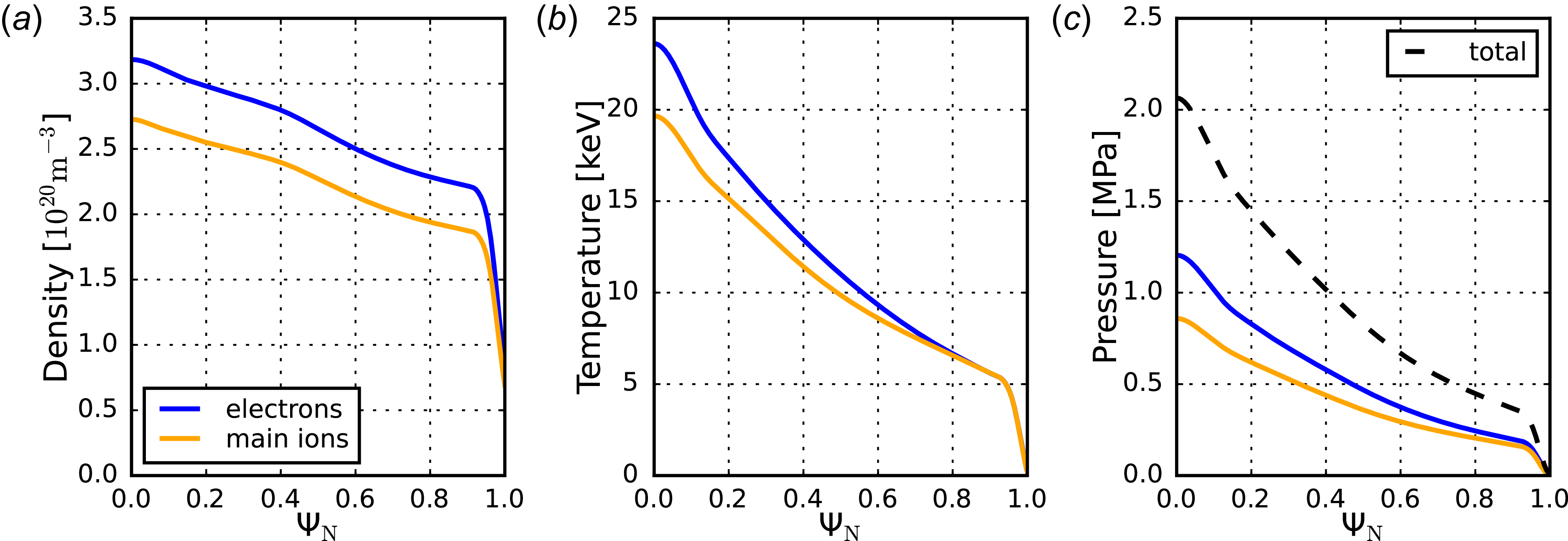


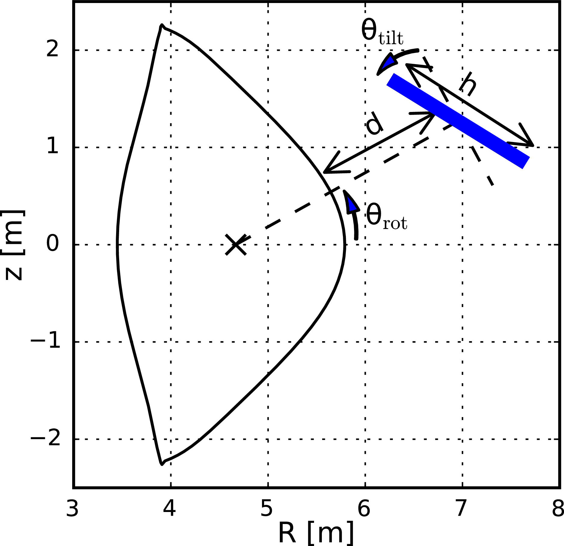


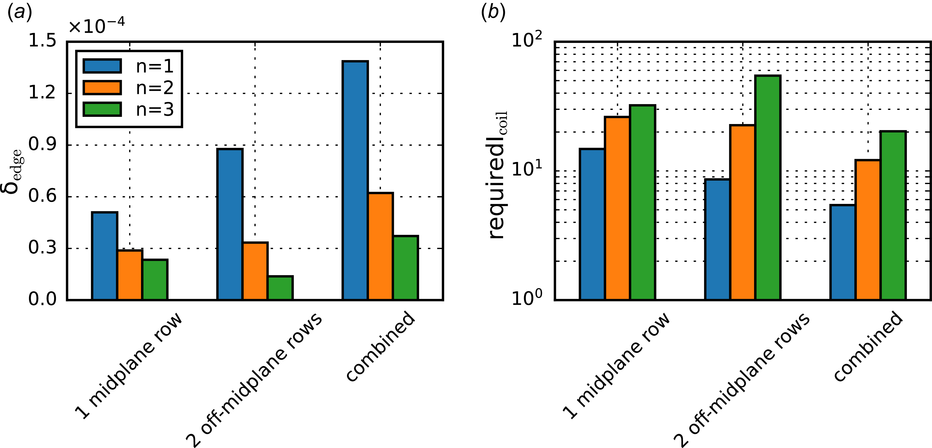


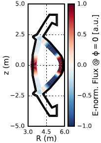
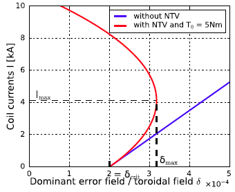


 Open access