


1. Introduction
The interaction of a rolling cylinder or wheel with a pool of liquid resting on a substrate is relevant to many practical problems such as roll coating, lubrication of bearings and rail transport. In rail transport, which primarily motivated this work, a pool of ‘liquid friction modifier’, a viscous liquid containing small amounts of microscopic solid lubricants like graphite, is deposited on the track ahead of the approaching train. Some of this liquid is picked up by the passing wheel and can reduce wheel and rail wear, noise and fuel consumption (Harmon & Lewis Reference Harmon and Lewis2016; Stock et al. Reference Stock, Stanlake, Hardwick, Yu, Eadie and Lewis2016; Rahmani & Green Reference Rahmani and Green2017). When the approaching wheel contacts this liquid pool, the lubrication pressure developed can be sufficient to raise the wheel slightly off the track. The fluid passes through this gap and splits at a downstream meniscus, with part of the fluid adhering to the wheel and part remaining on the track; ahead of the gap, the fluid accumulates in a bow wave (figure 1). The split film adhering to the wheel is conveyed further along where it may be deposited back onto the track in a subsequent carry-down process.
Sketches of the geometry for lubricated rolling over a viscous fluid layer, showing (a) the wheel rolling into the initial pool, and (b) the details of the lubrication film, with various physical parameters indicated. The axial direction is defined as the direction of the cylinder/substrate motion and the lateral direction is perpendicular to the page, along the cylinder width ( $z$-axis).

The lubricated rolling process illustrated in figure 1 is similar to the levitation problems considered by Eggers, Kerswell & Mullin (Reference Eggers, Kerswell and Mullin2013), Mullin, Ockendon & Ockendon (Reference Mullin, Ockendon and Ockendon2020) and Dalwadi et al. (Reference Dalwadi, Cimpeanu, Ockendon, Ockendon and Mullin2021), wherein a solid object is held aloft by a vertical moving belt coated with a thin layer of viscous fluid. The splitting of the film at the downstream meniscus also features in a great many other coating problems (Greener & Middleman Reference Greener and Middleman1975; Benkreira, Edwards & Wilkinson Reference Benkreira, Edwards and Wilkinson1981; Coyle, Macosko & Scriven Reference Coyle, Macosko and Scriven1986; Decré, Gailly & Buchlin Reference Decré, Gailly and Buchlin1995; Weinstein & Ruschak Reference Weinstein and Ruschak2004; Ascanio & Ruiz Reference Ascanio and Ruiz2006; Becerra et al. Reference Becerra, Romero, Azevedo and Carvalho2007). In particular, the associated two-dimensional flow is known to be prone to the so-called printer's instability, which generates a complicated three-dimensional filamentary structure (Pearson Reference Pearson1960; Pitts & Greiller Reference Pitts and Greiller1961). As will be shown in § 3.1, for the rolling flows considered here, the film splitting is complicated still further by the generation of substantial negative pressures that likely induce cavitation or de-gassing. Such cavitation in a lubrication setting has been observed by Taylor (Reference Taylor1963), Dowson & Taylor (Reference Dowson and Taylor1979) and others.
The purpose of the present paper is to provide an experimental study of the rolling process illustrated in figure 1. The apparatus is designed with the rail transport application in mind, reproducing some of the relevant physical conditions. However, we introduce a number of idealizations to better suit an interrogation of the underlying fluid mechanics. The apparatus consists of the blade of a band saw fitted with wheels and instrumentation. We take pressure measurements, use a proximity sensor to record the separation of the wheel and rail, and map out the depth of the film of fluid left on the track once the wheel rolls by using laser-induced fluorescence. We also image the bow wave and film splitting at the downstream meniscus using high-speed cameras and a borescope. The band-saw blade provides a relatively long flat track; up to six interactions between the wetted part of the wheel and rail are possible before the wheel returns to the original pool. Overall, the observations provide contemporaneous, quantitative measurements of various aspects of the rolling dynamics, which can be combined to build a relatively complete picture of the lubrication process.
To complement the experiments we also provide a theoretical model based on Reynolds lubrication theory. The analysis broadly follows that provided by Eggers et al. (Reference Eggers, Kerswell and Mullin2013), Mullin et al. (Reference Mullin, Ockendon and Ockendon2020) and Dalwadi et al. (Reference Dalwadi, Cimpeanu, Ockendon, Ockendon and Mullin2021), although here we must also deal with the finite width of the wheel, which permits significant amounts of fluid to leak out sideways. We make further simplifications by introducing some cruder approximations at the bow wave and downstream meniscus. In previous work on the two-dimensional version of the problem, matched asymptotic expansions are exploited to treat those regions more accurately than in the lubrication analysis, which formally breaks down owing to sharp streamwise gradients. The matched asymptotics allow one to incorporate a more faithful representation of the bow wave and film splitting, albeit at the expense of treating the full fluid mechanical problem at these locations (Ruschak Reference Ruschak1982; Coyle et al. Reference Coyle, Macosko and Scriven1986; Taroni et al. Reference Taroni, Breward, Howell and Oliver2012; Dalwadi et al. Reference Dalwadi, Cimpeanu, Ockendon, Ockendon and Mullin2021). Rather than dealing with such complications, and because the flow under the rolling wheel inevitably becomes three-dimensional (particularly at film splitting) and may cavitate, we opt for the cruder approach of replacing these finely scaled regions by simple, but plausible boundary conditions on the lubrication theory along the lines discussed by Coyle et al. (Reference Coyle, Macosko and Scriven1986).
The details of our experimental arrangement are provided in § 2, with additional discussion of some of the components given in the appendices. A summary of the key findings is provided in § 3. The complementary theoretical model is derived and compared against the experimental results in § 4. Our conclusion in § 5 includes a discussion of the open questions arising from this research.
2. Experimental details
As sketched in figure 2, the experimental arrangement consists of the blade of a woodworking band saw fitted with wheels, motors, pneumatic air cylinders and sensors. The band-saw blade provides a long and continuous moving flat track. The wheels were machined from mild steel and had a radius of  $R=10$ cm; four different widths of $W=2$, 5, 10 and 20 mm were used. The wheels were loaded by means of pneumatic air cylinders that were controlled by fast-acting solenoid valves. Two magnetic Hall effect sensors, with a 15 kHz sampling rate, measured the speed $U$ of the blade and wheel. A 2 kN load cell measured the normal force at the wheel–rail contact patch. The backing wheel was not driven and prevented any deflection of the blade under the applied normal load. Both wheels were mounted on a linear rail guide to ensure smooth and accurate activation. The parallelism of the wheel axle and the blade surface was verified by placing pressure-sensitive papers (Fujifilm Prescale HHS PS) between the wheel and the dry blade and observing the uniformity of the pressure distribution across the wheel width. To reduce the light reflection from the surface of the band saw blade (which is a requirement for the film thickness measurement technique, described later), the blade was chemically treated with black oxide (magnetite). The treated blade had a root-mean-square roughness of $850$ nm, measured by an optical profilometer. On the treated blade the two test liquids used in experiments, silicone oil and glycerin, had contact angles of $\theta _c=16\pm 3^{\circ }$ and $\theta _c=62\pm 4^{\circ }$, respectively (as measured by shadowgraphy, see Appendix A).
Schematic of the experimental apparatus, showing the wheel–rail interaction. The wheel on the left represents the train wheel and the blade represents the rail. The backing wheel provides support to prevent the deflection of the band saw blade under a large normal load. The load is applied through an air cylinder and various components measure the speeds and force.

A high-speed camera (Phantom V.12, with a resolution of  $512 \times 512$ pixels, and frame rates of 2000–5000 f.p.s.) and LED light source were used to image fluid flow upstream of the nip from the side. To observe the downstream meniscus, we used a 90 degree, 4 mm-diameter rigid borescope (MEDIT 9430E) coupled to a camera with illumination provided by two fibre optic lights (MO150-JH Technologies and MidoriTM-35 Watt).
To measure the instantaneous gap size between the wheel and the blade, a laser-based proximity sensor (Baumer OM20-P0026.HH.YIN), with a sampling rate of 5 kHz and an accuracy of 1  $\mathrm {\mu }$m, was mounted on the bed of the experimental apparatus. The sensor measured the distance to the wheel axle (shown in figure 2).
Pockets were machined in each quadrant of the largest (20 mm width) wheel to accommodate a small-scale piezoelectric gauge pressure transducer (Kistler, type 603CBA01000). The sensor has a rise time less than  $0.4\,\mathrm {\mu }$s, a natural frequency exceeding 500 kHz and a pressure range up to 1000 bar. To measure the lateral pressure distribution, 4 custom pressure taps, each 1 mm in diameter, were press fit into the wheel and the pressure transducer was connected to each tap in turn. A slip ring (SparkFun Electronics, ROB-13063) was used to transfer the electronic signal generated by the rotating pressure transducer from the rotating wheel. Further details of the pressure measurement system are provided in Appendix B.
At the start of each experiment a pool of liquid with a known thickness and length was applied to the blade. The pool length was varied from  $L_0=3$ to $L_0=80$ mm (typical value: $L_0=40$ mm) and the pool thickness was varied from $h_{in}=370$ to $h_{in}=1000\,\mathrm {\mu }$m (typical value: $h_{in}=500\,\mathrm {\mu }$m). The test liquid was either a water–glycerin solution or silicone oil. The water–glycerin solutions had dynamic viscosities of $\mu =0.73 - 1.19$ Pa s, density $\rho =1210\,{\rm kg}\,{\rm m}^{-3}$ and a fluid–air surface tension of $\gamma =60\,{\rm mN}\,{\rm m}^{-1}$. The silicone oil was characterized by $\mu =8.72$ Pa s, $\rho =950\,{\rm kg}\,{\rm m}^{-3}$ and $\gamma =21\,{\rm mN}\,{\rm m}^{-1}$. Trace amounts of a fluorescent dye (Rhodamine-B) were added to both liquids; several rheological experiments confirmed that the minute amount of added dye (0.04 % by mass) does not change the fluid viscosity.
To initiate the experiment, the speeds of the wheel and the blade, and the pneumatic cylinders operating pressure, were set. Once a photo diode sensor detects a marker on the blade, the pneumatic cylinders were activated, driving the wheel into contact with the blade upstream of the pool of liquid. The wheel then rolls over the liquid pool and picks up some of the liquid as it passes. One circumference downstream from the original pool, the liquid adhering to the wheel returns to the nip between the wheel and the blade, and the process repeats. The large length of the blade allowed six wheel–rail interactions before the wheel returned to the initial pool location. During the course of the experiments, the gap between the wheel and the blade, the fluid pressure, and the applied load were recorded. Once the experiment was complete, laser-induced fluorescence (LIF) of the deposited liquid was used to infer the film thickness. Details of the LIF technique are provided in Appendix A.
Experiments were carried out to study the effects of speed  $U$, load $L$ and viscosity $\mu$ on the rolling process. The wheel-blade speeds $U$ were varied between $0.2 - 8\,{\rm m\ s}^{-1}$, the fluid viscosities were varied from $\mu =0.73$ Pa s (water–glycerin solutions) to $\mu =8.72$ Pa s (silicone oil), and four different load-to-width ratios ( $L/W=11.2, 17.1, 38.8, 76.3\,{\rm kN}\,{\rm m}^{-1}$) were used.
3. Results
3.1. Interaction one
We refer to the passage of the wheel through the initial pool as Interaction One; Interactions Two and more refer to carry-down, where the liquid present on the wheel (from Interaction One) is subsequently transferred from the wheel back to the blade. The image on the left of figure 3(a) shows a typical example of the measured film on the band saw blade after Interaction One, and illustrates several aspects of the fluid mechanics of the lubricated rolling process. First, the finite depth of the film above the band on the track over which the wheel rolled highlights how the cylinder is lifted off that surface by the fluid pressure; the corresponding displacement recorded by the proximity sensor is shown in figure 4. The lubrication film extends both in front of the original pool, demonstrating how liquid is ploughed ahead of the rolling wheel, and also slightly behind it (a feature that is barely visible in figure 3(a), but more evident in other examples). The backward advance of the fluid edge results from the finite depth of the initial pool: contact between the wheel and fluid takes place before the location where the wheel touches the rail, and fluid is then pushed backwards into the small intervening gap (cf. figure 1a).
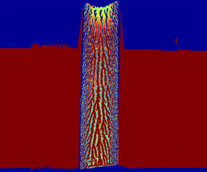
Deposited film thickness of six interactions for (a,b) silicone oil and (c) glycerin. The track is moving from top to bottom (equivalent to the wheel moving from bottom to top over a stationary track). Shown is a colour map of the liquid thickness in  $\mathrm {\mu }$m (the original pool is very deep, which causes the LIF signal to saturate in places). In (a), the wheel edge is not cleaned after first interaction; in (b,c), the wheel is cleaned. The dashed circles highlight sectors of the film over which the thickness pattern is reproduced during an interaction. Test conditions: $U=1\,{\rm m\ s}^{-1},\ L/W=11.2\,{\rm kN}\,{\rm m}^{-1},\ L_0=4\,{\rm cm}$, $h_{in}=500\,\mathrm {\mu }$m and $W=10$ mm.

The gap  $h_0$ between the wheel and track as measured by the proximity sensor. Also shown is the scaled thickness of the deposited fluid film on the track. Test conditions: $U=1\,{\rm m\ s}^{-1},\ L/W=11.2\,{\rm kN}\,{\rm m}^{-1},\ \mu =8.72$ Pa s (silicone oil), $W=10$ mm, $L_0=4$ cm and $h_{in}=500\,\mathrm {\mu }$m. The typical error bar of the gap measurement corresponds to the standard deviation of three experiments run under identical conditions.

In addition to the forward ploughing, liquid is also squeezed out to the side from the gap between the wheel and rail. This ‘side flux’ (the lateral spreading of liquid out of the nip caused by the high lubrication pressure) creates the two thin stripes bordering the ploughed-ahead film. Note that the initial pool is too deep for the side flux to be detected where the wheel rolls over the original pool, with the signal saturating there (red regions in figure 3).
Although the fluid-filled gap between the rail and wheel is constant across the width, the deposited film thickness forms a distinctive pattern. Indeed, as mentioned earlier, when a film of fluid passes through a narrow gap and splits at the meniscus, the film-splitting flow is prone to the printer's instability (Pearson Reference Pearson1960; Pitts & Greiller Reference Pitts and Greiller1961; Coyle, Macosko & Scriven Reference Coyle, Macosko and Scriven1990). For the typical Capillary number  $Ca=\mu U / \gamma$ and ratio of minimum gap $h_0$ to wheel radius $R$ encountered in our experiments ( $h_0/R \sim 0.001$), the splitting flow is expected to be unstable (Pitts & Greiller Reference Pitts and Greiller1961). The instability leads to a filamentation of the fluid film deposited on the track and wheel, as seen in figure 3(a), for the silicone oil. For the glycerin experiment shown on the left of figure 3(c) the interaction process is similar, with the film filamenting as it splits. This time, however, the glycerin filaments subsequently break and bead up on the blade surface, due to the higher surface tension and contact angle.
From the perspective of the lubrication dynamics of the rolling wheel, the patterning of the deposited films by the printer's instability is a distraction that can be eliminated by averaging the film thickness over an area exceeding the typical length scale of the filamentary structure. Such average film thicknesses for the first interaction are plotted against distance down the track in figure 4 and is compared with the proximity sensor measurements tracking the wheel position. For these examples, the film thickness is averaged laterally across the path of the wheel, and over sliding windows of length 0.25 cm in the direction of motion. Just after the wheel makes contact with the pool, the film thickness rises rapidly, then remains constant for a distance  $l_c$ (region II). The fluid ploughed ahead of the wheel supports the wheel for a further distance of $l_p$, over which the film thickness first decreases slowly (region III) before diminishing abruptly (region IV).
The average film thickness, when scaled by a suitable constant factor (of  $1.84$), closely tracks the wheel displacement. Thus, the take-off of the wheel from the deposited film does not substantially redistribute the fluid other than by creating the pattern of filaments, and the average film thickness consequently reflects primarily the wheel position. That said, however, some lateral redistribution of fluid does occur near the sides of the wheel, as illustrated in figure 5, which shows results for different wheel widths. In these tests, the ratio $L/W$ is held fixed, which would imply similar lubrication dynamics in the absence of side flux. However, the amount of side flux varies with the wheel width, which modifies the volume of fluid ploughed forwards and adjusts the minimum gap $h_0$ (figure 5b). The final take-off of the wheel from the film also introduces a distinctive decrease in film thickness towards the sides (figure 5c). The factor 1.84 minimizes the root-mean-square (r.m.s.) deviation between the film thickness deposited on the substrate and the instantaneous gap size measured in the constant film thickness regime for this particular experiment. This factor, which is an indication of the strength of the pressure-driven flow between the meniscus and nip, typically varies from 1.8 to 2 for various experimental parameters and pool depths, as discussed later in figure 14(f).
Variation of film thickness from Interaction One for different wheel widths. In (a) we show the thickness distribution calculated by averaging the LIF measurements over 2 mm square windows to eliminate the filament pattern resulting from the printer's instability, for  $W=10$ mm. In (b), we plot film thickness averaged laterally over the path of the wheel against distance along the track for four wheel widths. For (c), the film thickness is first averaged over the strip of length $l_c$, and then averaged laterally over running windows of length $0.2$ mm. Test conditions: $L/W=11.2\,{\rm kN}\,{\rm m}^{-1}$, $U=1\,{\rm m\ s}^{-1},\ \mu =8.72$ Pa s, $L_0=4$ cm and $h_{in}=500\,\mathrm {\mu }$m. Error bars correspond to one standard deviation of the data with three repeats.

Figure 6(a) displays the minimum gap observed for pools with different initial pool length  $L_0$. In agreement with figure 4, the steady gap is established after the wheel has run approximately 7 mm into the pool. For these test conditions, initial pools with $L_0\lesssim$ 7 mm cannot therefore reach steady state, as observed for the shortest two pools in figure 6(a). For $L_0\gtrsim 7$ mm, a steady state is attained over a distance $l_c$ depending on $L_0$, and the steady minimum gap $h_0$ and final ploughing length $l_p$ then become independent of pool length. For the remainder of this study, we consider pools that are significantly longer (typically $L_0=4$ cm) than the distance over which the wheel lifts up to ensure that the steady state is achieved.
(a) Gap size measurements for Interaction One vs the axial distance for different pool lengths when pool depth is constant,  $h_{in}=500\,\mathrm {\mu }$m, (b) film thickness for Interaction One, averaged laterally, vs the axial distance for different pool depths when pool length is constant, $L_0=4$ cm. The gap size (or equivalently film thickness) is constant over a distance $l_c$, and then declines over a ‘ploughing length’ $l_p$. Test conditions: $U=1\,{\rm m\ s}^{-1},\ L/W=11.2\,{\rm kN}\,{\rm m}^{-1},\ \mu =8.72$ Pa s (silicone oil) and $W=10$ mm. Error bars correspond to one standard deviation of the data with three repeats.

Figure 6(b) shows averaged film thicknesses for pools with different depth  $h_{in}$. The constant film thickness over $l_c$ is, to within experimental error, independent of the initial pool depth $h_{in}$ but depends on wheel speed, loading and width. The ploughing length $l_p$, however, increases with the pool depth due to the larger ploughed volume ahead of the wheel.
Observations of the bow wave and downstream meniscus during the first interaction are shown in figures 7 and 8. The two side views in figure 7 show the bow wave during and at the end of the passage through the initial pool. The bow wave forms a steep face lying some distance ahead of the minimum gap (figure 7a). Once the bow wave reaches the end of the pool, the side profile changes and the position recedes to the minimum gap (figure 7b). Measurements of the bow-wave position as a function of time show that  $x_l$ generally follows the trend of gap size shown in figure 4: $|x_l|$ increases quickly initially as fluid rapidly accumulates ahead of the wheel, generating the lift force that raises the wheel until the incoming flux matches that underneath the wheel. Over the ensuing steady state, $x_l$ remains roughly constant, before falling in the same fashion as $h_0$ once the wheel reaches the end of the pool. Images from the borescope clearly reveal the filamentation produced by the printer's instability at the downstream meniscus (figure 8); the typical distance between fluid filaments in the image matches that inferred from film thickness measurements (see below), to within 10 %.
High-speed images of the upstream fluid–air interface when the wheel is (a) midway through, and (b) beyond the initial pool. Also indicated is the position  $x_l$, relative to the minimum gap, where the bow wave contacts the wheel. Test conditions: $U=1\,{\rm m\ s}^{-1},\ L/W=11.2\,{\rm kN}\,{\rm m}^{-1},\ \mu =8.72$ Pa s (silicone oil), $W=20$ mm and $h_{in}=500\,\mathrm {\mu }$m.

Borescope image of the film-splitting meniscus, showing the fluid filaments in the lateral direction and the filamented pattern in the deposited films. The top surface is the rotating wheel and the bottom surface is the moving rail. The borescope was positioned approximately 3 cm downstream the minimum gap location. Test conditions:  $U=1\,{\rm m\ s}^{-1},\ L/W=11.2\,{\rm kN}\,{\rm m}^{-1},\ \mu =8.72$ Pa s (silicone oil), $W=20$ mm and $h_{in}=500\,\mathrm {\mu }$m.

Pressure measurements during the first interaction are shown in figure 9. Substantial lubrication pressures are encountered as fluid moves towards the minimum gap; just beyond the nip, the pressure falls substantially and becomes sub-atmospheric. Note that pressure traces in figure 9 and other figures are all gauge pressure measured relative to atmospheric pressure (i.e.  $p=0$ corresponds to the atmospheric value). The sub-atmospheric pressure (visible in inset of figure 9a), of the order of the vapour pressure, is likely an indication of cavitation or degassing. For reference, silicone oil and glycerin have vapour pressures of ${<}1.3$ kPa and ${<}0.05$ kPa absolute at $25\,^\circ$C, respectively (Ross & Heideger Reference Ross and Heideger1962; Yaws Reference Yaws2015). Pressures are almost constant for the middle two pressure ports ( $z=0,2.5$ mm), but drop nearer the edge of the wheel (figure 9b). The implied lateral pressure gradient drives the side flux and may play a role in the redistribution process at take-off that leads to the lateral variation of film thickness in figure 5. For the three test conditions shown in figure 9(b), the pressure profile is slightly flatter and falls more quickly towards the sides for wheels that are relatively wider, as quantified by the length scale ratio, $W/\sqrt {Rh_0}$, a dimensionless parameter that we employ in § 4.
(a) Axial pressure variation at different lateral locations for  $U=1\,{\rm m\ s}^{-1},\ L/W=11.2\,{\rm kN}\,{\rm m}^{-1},\ \mu =8.72$ Pa s and $W=20$ mm. (b) Variations of the normalized peak pressure in the lateral direction for multiple test conditions at constant width $W=20$ mm. The peak pressure is normalized by centreline pressure for each test condition. The peak pressures vary by a factor of almost 3 for test conditions in (b), from 1.6 MPa for $U=2\,{\rm m\ s}^{-1}$, $L/W=11.2\,{\rm kN}\,{\rm m}^{-1}$ to 5.0 MPa for $U=1\,{\rm m\ s}^{-1}$, $L/W=22.4\,{\rm kN}\,{\rm m}^{-1}$. Test fluid is silicone oil.

3.2. Higher interactions
Figure 3 also displays film thicknesses for higher interactions. Turning first to the silicone oil experiment shown in figure 3(a), we see that the fluid left on the running track reduces in depth each time the film splits, weakening the filamented pattern left behind. Also, the side flux during Interaction One leaves fluid adhering to the sides of the wheel, which then transfers back on to the track in subsequent revolutions to reproduce the stripes on either side of the running band. To verify that fluid did not re-enter the gap from the sides during the higher interactions, we conducted other experiments in which the experiment was immediately stopped after the first wheel–rail interaction, the sides of the wheel cleaned, and the experiment resumed with liquid only present on the contact band of the wheel. Figure 3(b) displays the repeat of the experiment in figure 3(a), but with the sides of the wheel cleaned after Interaction One. The two tests have comparable average film thicknesses on the running band, verifying that an insignificant amount of fluid is transferred back from the sides of the wheel during the higher interactions.
As highlighted by the dashed circles also drawn in figure 3(b,c), the patterns for higher interactions contain common features between consecutive interactions. To explore this observation further, we cross-correlate the images, with the results shown in figure 10. This analysis indicates that Interactions One and Two have relatively small peaks in correlation coefficients (0.13 for silicone oil and 0.08 for glycerin) for spatial shifts that are located far from the centre of the images. On the other hand, the interaction pairs Three/Four and Four/Five have relatively large peak correlation coefficients (of 0.85 or 0.92 for silicone oil, and 0.69 and 0.58 for glycerin), occurring at the centre of the images. Interactions Two and Three are somewhere between, having correlation coefficients of 0.15 or 0.24 at zero spatial shift. This leads us to conclude that the higher interactions are strongly correlated (taking this to be implied by peak values above 0.5 at zero spatial shift), the first and second interactions are essentially uncorrelated, and interactions Two and Three are perhaps weakly correlated.
Cross-correlation of the experimental images (from figure 3) between different interactions for (a) silicone oil and (b) glycerin. As an example, Column ‘12’ refers to the cross-correlation between Interaction pair One/Two;  $U=1\,{\rm m\ s}^{-1},\ L/W=11.2\,{\rm kN}\,{\rm m}^{-1}$, $W=10$ mm and $h_{in}=500\,\mathrm {\mu }$m.

The cross-correlation map for silicone oil has negative peaks a short distance to the left and right of the peak coefficient, followed by secondary peaks at twice that distance to either side. These secondary peaks arise from the characteristic length scale present in the pattern of the deposited film in each image, namely the separation between the filaments. The length scale estimated from the cross-correlation is in agreement with direct visual observations using the borescope, as mentioned earlier. For glycerin, however, the secondary peaks are not present because the beading up on the surface generates a largely random pattern of droplets that cannot be aligned for any non-zero spatial shift.
The cross-correlation analysis implies that the pattern in the deposited film is reproduced during the higher interactions, where the liquid layer on the wheel is thin. Evidently, in these interactions, the fluid film is not squeezed back into a uniform sheet by the passage of the wheel. Otherwise, it would suffer another film-splitting instability to generate an uncorrelated pattern. Instead, the existing filaments or droplets must retain their shape and become evenly split and ‘printed’ back on the blade after passage through the nip. The fluid mechanics of this ‘printing’ process is very different from that sketched in figure 1(b).
Given that the radius of curvature of the wheel is relatively large ( $R/h_0>1000$), one expects the film splitting at the meniscus to be almost symmetric, with equal amounts of fluid coating the blade and adhering to the wheel. Indeed, by placing aluminium strips on the blade and wheel, it was possible to directly measure the mass of the split films. The split masses after each interaction were equal to within the experimental error, indicating a symmetric film split.
In view of the symmetrical film split, if there is no side flux, the net mass of the lubrication film on the blade for Interaction  $i$ should be exactly half the mass at Interaction $i-1$. Figure 11 is a plot of twice this mass ratio. The lubricated film mass for Interactions Two and Three is somewhat less than half that at the previous interaction, and the discrepancy identifies side flux. The side flux is obviously important for Interaction One, but cannot be directly measured as the side flux is pushed into the original pool. For Interactions Four and above, the side flux is insignificant. Referring to figure 3(b), one can alternatively calculate the side flux by measuring the mean thicknesses (and thus mass) of the two long strips adjacent to the lubrication film at Interaction Two. This alternative calculation agrees with the direct mass measurements to within experimental error.
Mass  $m_{i{th}}$ left on the blade after Interaction $i$ multiplied by two and divided by this mass at the previous interaction plotted against $i$. Test conditions are $\mu =8.72$ Pa s and $W=10$ mm. Experiments are averaged over three repetitions and the error bars correspond to one standard deviation of the data.

3.3. Wheel lift-off
Although the wheel was pushed off the substrate to deposit a fluid film with finite average thickness in many of our experiments, such lift-off did not always occur. As illustrated in figure 12, the wheel failed to take off at relatively low speed or high load, leaving behind a film with a thickness that was undetectable by the LIF technique. This figure presents experimental film thicknesses averaged over width and the strip of constant depth with length  $L_c$ for different speeds (a) and loads (b). Note that, as expected from previous discussion, when the wheel lifts off, the deposited film thickness falls by almost a factor of two between interactions. Moreover, for the first interaction, the thickness is roughly proportional to speed and inversely proportional to load (the depth falls by close to a factor of two as the speed is adjusted from 8 to $4\,{\rm m\ s}^{-1}$ in figure 12(a), then increases by a similar factor when the load decreases from 38.8 to $17.1\,{\rm kN}\,{\rm m}^{-1}$ in (b)).
Film thickness vs interaction number for (a) varying speed  $U$, with a glycerin–water mixture, and (b) varying load, with silicone oil. The initial pool has depth $h_{in}=500\,\mathrm {\mu }$m and length $L_0=4$ cm. The error bars correspond to one standard deviation of the data with three repeats.

One might expect that lift-off fails to occur when the minimum gap required for the fluid flow to build up the lubrication pressure to balance the wheel load becomes smaller than the roughness scale of the solid surfaces, as in bearings (Vogelpohl Reference Vogelpohl1965; Lu & Khonsari Reference Lu and Khonsari2005). To test the possibility that lift-off was sensitive to surface roughness, thin metal shims were roughened to differing degrees and attached to the blade (creating surfaces with r.m.s. roughness scale  $\epsilon =2.60,4.30\,\mathrm {\mu }$m, note that the original blade has a roughness $\epsilon =0.85\,\mathrm {\mu }$m). The roughness of each shim was measured using an optical profiling system. The liquid was then pooled on top of the shims, and the experiments were conducted as for the original blade surface. To better show the dependence of the lift-off as a function of speed, load and surface roughness, we combine the data from Interaction One for various speeds and loads, and plot them against ${\mu U R W}/{L}$ in figure 13. As we explain in § 4 below, ${\mu U R W}/{L}$ is the primary scaling of the minimum gap predicted by lubrication theory. The graph also includes measurements for different rough shims. The extrapolation of the film thickness (black dashed line) shows the expected film thickness for smaller values ${\mu U R W}/{L}$ (equivalently lower speeds or higher loads). For instance, for the case $U=1\,{\rm m\ s}^{-1}$ in figure 12(a) (corresponding to ${\mu U R W}/{L} \approx 10\,\mathrm {\mu }$m), the expected film thickness is $h_{out} \approx 10\,\mathrm {\mu }$m, though the thickness was undetectable in the experiments. It is clear that extrapolation from higher speeds results in a film thickness well above the detection limit of LIF, so if lift-off were to happen, it should be detectable. Moreover, no difference was observed in the conditions for lift-off when the surface was rough, leading us to conclude that surface roughness did not play any role in lift-off. In fact, the tests suggested that for the first interaction, lift-off usually occurred provided that
 \begin{equation} \frac{\mu U R W}{L} > 19\,\mathrm{\mu}{\rm m}. \end{equation}
The criterion in (3.1) is equivalent to one on the minimum gap  $h_0$ and implies a threshold that is far larger than the surface roughness scale. Indeed, for some of the cases without lift-off conducted on the original blade surface, gravimetric measurements of the small amount of liquid that does pass through the nip and becomes left on the blade indicates an average thickness of about $400$ nm, with the fluid filling the valleys created by the surface roughness rather than forming a continuous sheet. Thus, in these situations, metal-to-metal contact likely occurs between the wheel and track and lubrication pressures are evidently insufficient to counter the applied load and lift the wheel. A similar situation arises for hydro-planing, although the Reynolds numbers reached there are much higher, and the surface topography of the wheel plays an important role (Kulakowski & Harwood Reference Kulakowski and Harwood1990; Seta et al. Reference Seta, Nakajima, Kamegawa and Ogawa2000; Löwer et al. Reference Löwer, Wagner, Unrau, Bederna and Gauterin2020).
Lift-off threshold during Interaction One as a function of speed, load and surface roughness. Also shown on the graph are the detection limit of LIF and the film thickness extrapolation from higher speeds.

Somewhat surprisingly, the criterion in (3.1) is clearly violated for many of the higher interactions of the cases with lift-off in figure 12. The reason for this disagreement is not apparent, although the cross-correlation analysis performed in § 3.2 highlights how the higher interactions do not take place with the formation of a continuous lubrication film. Rather, the filamentary pattern generated by the printer's instability becomes printed between interactions. Perhaps this spatial inhomogeneity is sufficient to permit lift-off in cases where a continuous film of the same amount of fluid cannot generate the required lubrication pressure.
4. Lubrication analysis
Our observations suggest that, when the wheel lifts off, a steady lubrication film is quickly established underneath the cylinder that provides the lift force to counter the load. The steady lubrication continues until the fluid that is ploughed forwards reaches the end of the reservoir entering the gap. In this section, we exploit standard lubrication theory to provide a model for the steady lubrication layer, ignoring the final thinning of the film and touchdown of the wheel back on to the track. We then compare the predictions of the theory with our experimental observations.
4.1. Mathematical formulation
As illustrated in figure 1, we use a Cartesian coordinate system  $(x,y,z)$ to describe the geometry, in which the $x$-axis points in the forwards direction and the $y$-axis is perpendicular to the rail. We consider the fluid in the nip region from the location of the bow wave $x=x_l$ to the downstream separation at the meniscus $x=x_m$. Over this region, the gap $h$ in the $y$-direction is much smaller than both $W$ (width) and the length scale $\sqrt {Rh_0}$ characterizing variations in the $x$-direction. The leading-order expressions of mass conservation and force balance then demand
 $$\begin{gather} u_x + v_y + w_z = 0, \end{gather}$$
 $$\begin{gather}p_x = \mu u_{yy}, \end{gather}$$
 $$\begin{gather}p_y = 0, \end{gather}$$
 $$\begin{gather}p_z = \mu w_{yy}, \end{gather}$$
where the fluid velocity and pressure are  $(u,v,w)$ and $p$ (respectively), and we have used subscripts as a short-hand notation for partial derivatives. Here, we have neglected gravity, in view of the high pressures experienced underneath the wheel, and inertia, because the Reynolds number for typical experimental conditions is low ( $Re=\rho U h_0 / \mu =O(10^{-2})$ for $\rho =10^3\,{\rm kg}\,{\rm m}^{-3}$, $U=1\,{\rm m\ s}^{-1}$, $h_0=10^{-4}$ m and $\mu =10$ Pa s).
The positions,  $x_l$ and $x_m$, as well as the minimum gap $h_0$ are not known at the outset, but must be determined as a part of the solution to the lubrication equations after the imposition of suitable boundary conditions. On the rail and wheel we have no slip
 $$\begin{gather} u=U \quad {\rm and} \quad v=w=0 \quad {\rm at} \ y=0, \end{gather}$$
 $$\begin{gather}u=U,\quad v=Uh_x \quad {\rm and}\quad w=0 \quad {\rm at} \ y=h. \end{gather}$$
Our observations of the free surface profile upstream demonstrate that the bow wave is too steep to be modelled by the lubrication mechanism (figure 7). Therefore, we treat this region as infinitely narrow and replace the bow wave by a discontinuity in depth, applying continuity of mass (i.e. flux) across the resulting shock. Because typical capillary numbers are large ( $Ca=\mu U / \gamma = 10^2$ for surface tensions $\gamma$ of order $0.1\,{\rm Nm}^{-1}$), we also neglect surface tension and set the pressure to the atmospheric value $p_{atm}$.
Any treatment of the downstream meniscus is more complicated in view of the severe low pressures that are achieved there, the cavitation or de-gassing that likely results, and the ever-present printer's instability. We avoid such complications by assuming that the printer's instability does not affect the net flow across the meniscus region, and that the fluid cavitates at its vapour pressure  $p=p_{vap}$ here with zero pressure gradient. Note that if we do not limit the pressure in this way, but continue the lubrication flow further along to a separation point of the kind considered by Ruschak (Reference Ruschak1982), Coyle et al. (Reference Coyle, Macosko and Scriven1986) and Dalwadi et al. (Reference Dalwadi, Cimpeanu, Ockendon, Ockendon and Mullin2021), then unphysically large negative pressures are generated.
4.2. Reduction
Equation (4.3) implies that the pressure is independent of  $y$; in view of the boundary conditions in (4.5a,b)–(4.6a–c), we may then integrate (4.2) and (4.4) to find the velocity components $u$ and $w$ together with their associated flow rates. The integral of (4.1) across the gap then leads to the Reynolds equation,
 \begin{equation} \frac{\partial}{\partial x} \left( Uh - \frac{h^3}{12\mu}p_x\right) - \frac{\partial}{\partial z} \left( \frac{h^3}{12\mu}p_z\right)= 0, \end{equation}
where
 \begin{equation} h \approx h_0 + \frac{x^2}{2R}. \end{equation}
In general settings, the solution of (4.7) is complicated by the unknown locations of the curves along the  $(x,z)$-plane identifying the bow wave and downstream meniscus. As our treatment of these locations is rudimentary anyway, to avoid such complications, we adopt a cruder approach. In this approach, we assume that the wheel is sufficiently wide that the pressure distribution remains close to that of the two-dimensional problem. With this assumption, the bow wave and downstream meniscus follow approximately straight lines ( $x_l$ and $x_m$ are independent of $z$), and we may solve (4.7) more simply. The key is to first integrate the equation over the wheel width, assuming symmetry about the centreline $z=0$
$z=0$
 \begin{equation} \frac{\partial}{\partial x} \left( Uh - \frac{h^3}{12\mu} {\bar{p}}_x \right) = \left[ \frac{h^3}{6\mu W} p_z \right]_{z=({1}/{2})W},\end{equation}
where
 \begin{equation} {\bar{p}} = \frac{2}{W} \int_0^{({1}/{2})W} (p-p_{atm}) \,{\rm d} z. \end{equation}
To relate the lateral pressure gradient at the edge to the average pressure  ${\bar {p}}$, we employ the approximation,
 \begin{equation} \left[ p_z \right]_{z=({1}/{2})W} ={-} \frac{{\bar{p}}}{\varDelta}, \end{equation}
where  $\varDelta$ denotes the characteristic length scale in $z$ over which the pressure falls to its atmospheric value as we approach the side of the wheel. For relatively wide wheels for which the width W is irrelevant, and without the input of any further physics applying at the edge, the only choice for this length scale is $\sqrt {Rh_0}$. So, we take $\varDelta = C \sqrt {Rh_0}$, where $C$ is a dimensionless constant that must be calibrated by other means. Hence
 \begin{equation} \frac{\partial}{\partial x} \left( Uh - \frac{h^3}{12\mu} {\bar{p}}_x \right) ={-} \frac{h^3}{6\mu W \varDelta} {\bar{p}}. \end{equation}
Note that the right-hand side of (4.12) models the loss of fluid at the edges of the wheel; i.e. the side flux. For an infinitely wide wheel  $W\to \infty$, this term disappears (two-dimensional lubrication) and the equation can be integrated analytically to find the pressure distribution (e.g. Coyle et al. Reference Coyle, Macosko and Scriven1986).
Having eliminated the dependence on the lateral coordinate  $z$ in this fashion, we must next impose the boundary conditions at $x_l$ and $x_m$, including an average across the wheel. In particular, at the bow wave we impose
 \begin{equation} {\bar{p}}(x_l) = 0 \quad {\rm and} \quad Q_{in} = Uh_{in} = \left[U h - \frac{h^3}{12\mu} {\bar{p}}_x\right]_{x=x_l}, \end{equation}
and at the downstream meniscus,
 \begin{equation} {\bar{p}}(x_m) = p_{vap} - p_{atm} \quad {\rm and} \quad {\bar{p}}_x(x_m) = 0. \end{equation}
Finally, the force balance on the wheel dictates that the net lubrication pressure must balance the applied load
 \begin{equation} \frac{L}{W} = \int_{x_l}^{x_m} {\bar{p}} \,{\rm d}\kern0.7pt x. \end{equation}
The second-order differential equation (4.12) in combination with the five conditions (4.13a,b)–(4.15) determines the average pressure distribution  ${\bar {p}}(x)$ together with the unknown parameters $x_l$, $x_m$ and $h_0$. For this task, we solve the equations numerically, employing MATLAB's in-built boundary-value solver, BVP4C.
4.3. Sample solutions
To provide some physical insight into the solutions of the model, we display a family of solutions in figure 14. For this, we fix the wheel geometry and speed ( $R$,
$R$,  $W$ and $U$), the fluid properties ( $\mu$ and $p_{vap}$) and the applied load $L$, but vary the incoming flux $Q_{in}$ by adjusting the incoming pool depth $h_{in}$. The dimensionless constant $C$ is taken to be $0.87$ (the rationale for this choice is provided in § 4.4).
Model solutions for varying initial pool depth  $h_{in}$. The solid (blue) curves show result for $W=1$ cm; the dashed (red) lines show results for an infinitely wide wheel. In (a) we plot a selection of pressure profiles for $h_{in}=50,200,1000\,\mathrm {\mu }$m (solution for an infinitely wide wheel is not possible for $h_{in}$ beyond ${\sim }350\,\mathrm {\mu }$m, therefore two red curves correspond to $h_{in}=50,200\,\mathrm {\mu }$m). Below, against $h_{in}$, we plot (b) $h_0$, (c) $x_m$ and (d) $x_l$. In (e) and (f), for the model with $W=1$ cm, we respectively plot the fraction of fluid that is diverted to the sides and the ratio $h_0/h_{out}$. For (b,d,e,f), we include results from tests conducted at the same experimental parameter settings, showing the gap size, $x_l$, side-flux fraction and $h_0/h_{out}$ during the first interaction for a pool with initial depth $h_{in}=1000\,\mathrm {\mu }$m, and then those variables (except $x_l$) for all six interactions for a pool with $h_{in}=500\,\mathrm {\mu }$m. The bow wave does not form after Interaction Two due to printing, therefore $x_l$ is plotted only for the first two interactions in (d). Here, $U=1\,{\rm m\ s}^{-1},\ L/W=11.2\,{\rm kN}\,{\rm m}^{-1},\ \mu =8.72$ Pa s, $C=0.87$, $p_{vap}-p_{atm}=-0.1 MPa$. The error bars correspond to one standard deviation of the data with three repeats.

For low incoming fluxes, the fluid cannot build up appreciably in front of the minimum gap. As a result, the wheel descends close to the rail, with the decrease in  $h_0$ offsetting the relatively small wetted length ( $x_m-x_l$) to raise the net lubrication pressure. As the flux is increased, the wheel sits further from the rail and the wetted length increases. For somewhat higher fluxes, the wetted length continues to increase, but the minimum gap $h_0$ and meniscus position $x_m$ level off. This feature reflects how the pressure distribution becomes largely independent of $h_{in}$ once the incoming flux is sufficiently large, and so the load can be balanced without changing $h_0$. The higher fluxes are compensated chiefly by an increase in the upstream length $|x_l|$. The increased wetted length enhances the side flux, whilst permitting the flow through the nip to remain unchanged.
For comparison, figure 14 also shows corresponding results for an infinitely wide wheel ( $W\to \infty$). In this case, steady force balance cannot be maintained for all $h_{in}$. Below a threshold flux, steady states are possible with a finite wetted length; i.e. ‘planing states’, as observed when the wheel has finite width and there is side flux. By contrast, above the threshold, the incoming flux is too high to permit steady force balance. Instead, the steady solution disappears and we anticipate a ‘flooding state.’ In a flooding state, the upstream length continually increases with time, all the while maintaining the same minimum gap.
A key feature of the solutions for typical experimental parameter settings is that the peak gauge pressures near the nip are far larger than the pressure at which the fluid cavitates. Consequently,  ${\bar {p}}$ becomes small at $x=x_m$, and the solution becomes insensitive to the precise pressure imposed at the downstream meniscus (as long as it remains small). In this setting, in view of (4.12), we then expect the pressure to scale as $\mu U R^{1/2} h_0^{-3/2}$ (the usual pressure scale for a journal bearing or rolling cylinder). However, the pressure also depends on the length scale ratio ${\mathcal {R}}=Rh_0/(W\varDelta )$ (from the side-flux term) and the dimensionless incoming flux $\lambda = Q_{in}/(Uh_0)$, which mostly controls the position of the bow wave. Thus, the load condition implies a scaling of the form
 \begin{equation} h_0 \sim \frac{\mu U R W}{L}I\left({\mathcal{R}}, \lambda \right), \end{equation}
where the dimensionless factor  $I$ incorporates the relative effect of side flux and the bow-wave position. This scaling is unfortunately implicit because $\mathcal {R}$ and $\lambda$ depend on $h_0$. Nevertheless, when the wheel is wide and the wetted length is sufficiently large, the pressure distribution becomes insensitive to $x_l$. In that case, $I$ is approximately constant and (4.16) identifies the main dependencies of the minimum gap on the experimental parameters. Even if the wheel is not wide and the wetted length is not large (so that the problem remains sensitive to the incoming flux), the minimum gap is expected to depend only on load and viscosity through the combination $L/\mu$. The dependence on wheel width and speed is more convoluted, as changing those parameters affects the wetted length and degree of side flux.
4.4. Calibration of  $C$
$C$

Our method for dealing with side flux in the model introduces a free parameter  $C$ that requires calibration. For this task, for each of the tests that we conducted, we match the experimental parameters and then find (using Newton iteration) the value of $C$ for which the theoretical prediction for the final deposited film thickness $h_{out}$ matches that measured experimentally. Although $h_{out}$ does not appear in the lubrication equations (unlike $h_0$), one can infer it from the minimum gap by using the flux balance at the meniscus $h_{out}=({\lambda _m}/{2}) h_0$, where $\lambda _m$ is the non-dimensional axial flux at the meniscus that is predicted by the model. The resulting values of $C$ are plotted against ${W}/{\sqrt {Rh_0}}$ in figure 15(a). Three regions are identified on this graph: for relatively wide wheels with ${W}/{\sqrt {Rh_0}}>9$ (labelled III in the figure), there is much scatter in the fitted values of $C$. This scatter reflects how the side flux for such cases is small, and any attempt to fit the corresponding parameter $C$ of the theory is suspicious. In addition, this is also the region where printing interactions can occur and the model does not apply. For moderate wheel widths, $2.5<{W}/{\sqrt {Rh_0}}<9$ (region II in the figure), the scatter in the fitted values of $C$ is less and the experiments support the parameterization of the model, $\varDelta = C \sqrt {Rh_0}$ with $C \approx 0.87$. At yet lower wheel widths ${W}/{\sqrt {Rh_0}}<2.5$ (labelled I in the figure), the fitted values for $C$ depend systematically on the ratio ${W}/{\sqrt {Rh_0}}$. For such narrow wheels, we conclude that the parametrization $\varDelta \sim \sqrt {Rh_0}$ is poor, owing to significant lateral pressure gradients and side flux. An alternative for these cases is to use the wheel width $W$ for the length scale $\varDelta$ over which the pressure declines near the side of the wheel. As shown in figure 15(b), the alternative parameterization $\varDelta = C' W$ with $C'\approx 0.36$ (or $C=C'({W}/{\sqrt {Rh_0}})$) performs better here. In view of these findings, to complete the model, we set
 \begin{equation} \varDelta=\begin{cases} C'W\approx0.36W & \text{for}\ \dfrac{W}{\sqrt{Rh_0}}<2.5 \\ C\sqrt{Rh_0}\approx0.87\sqrt{Rh_0} & \text{for}\ \dfrac{W}{\sqrt{Rh_0}}>2.5 \end{cases}. \end{equation}
(a) Fits of the constant  $C$ as a function of the ratio ${W}/{\sqrt {Rh_0}}$. Three distinct regions are identified based on whether the fitted values depend systematically on ${W}/{\sqrt {Rh_0}}$ (I), are independent of this ratio (II) or inaccurately identified because side flux is low (III). In (b) the results for ${W}/{\sqrt {Rh_0}}<2.5$ are replotted, scaling $C$ with ${W}/{\sqrt {Rh_0}}$.

4.5. Comparison of theory and experiments
The performance of the calibrated model in predicting the final average film thickness is shown in figure 16. Figure 14 also makes a direct comparison of the theory and experiment for a particular pair of tests. In figure 16, we include results from all the interactions from experiments conducted with different pool depths, pool lengths, wheel widths, velocities, fluid viscosities and loadings. For comparison, we also show the corresponding results in which the side flux is neglected (labelled as ‘No side flux,  $C=0$’). That version of the model is insufficient to reproduce the observations, particularly for the first interaction. By contrast, for the full model (labelled as ‘Parameterization (4.17)’), the r.m.s. discrepancy between the model and the experiments is 5.9 %, which is comparable to the experimental error. Note that, strictly speaking, the model cannot apply to Interaction Three and higher, owing to the switch of the dynamics for these interactions to printing. Nevertheless, the model continues to perform well, simply because it predicts a weak fluid flow under the wheel and an equal split of the film between wheel and rail, leading to $h_{out}=\frac 12 h_{in}$, as for printing. As evident from figure 3, the fluids used in this study (silicone oil and glycerin) have different wetting properties. However, according to figure 16, which includes measurements for both fluids, the role played by the wetting characteristics is insignificant in our problem as the scaling ${hL}/{\mu URW}$ is successful in collapsing all the experimental data.
Scaled film thicknesses  $h_{out}L/(\mu U R W)$ predicted by the model plotted against those measured experimentally. The model results labelled ‘ $W \rightarrow \infty$’ are calculated ignoring any side flux; those labelled ‘Finite W’ are for the full model using the calibration in (4.17). Different colours represent film thicknesses for different interactions. For example, 1st and 2nd refer to the Interactions One and Two, and so on. The inset magnifies the results for Interactions Four to Six.

Although the agreement in figure 16 is satisfying, the predictive power of the model is offset by the need for the calibration in (4.17). A more demanding test of the model is shown in figure 17. This figure compares measured and predicted average pressure profiles  ${\bar {p}}$ for the wide wheel ( $W=20$ mm) for three different parameter settings. For this comparison, the experimental pressure profiles from the four ports across the wheel (at $z=0$, $2.5$, 5 and 7.5 mm), shown in figure 9, are integrated by the trapezoid rule. We further assume that the pressure distribution is symmetrical about the centreline $z=0$ and that $p=p_{atm}$ at the sides. In addition to the pressure distribution comparisons of figure 17, we also made measurements for other test settings. In all cases, the model reasonably matches the observations, with differences of 8 % and 2 % in the peak and net pressures, and a comparable mismatch in the apparent wetted length. However, the observations of the lateral pressure gradients at the wheel edge in figure 9(b) do not fully support the parameterization in (4.11) with $\varDelta = C\sqrt {Rh_0}$ (the observed pressure profiles are little different, even though $\sqrt {Rh_0}$ varies by a factor of approximately two).
Experimental (dashed) and theoretical (solid) pressure profiles, averaged across the wheel and plotted against distance down the track. Other test conditions:  $\mu =8.72$ Pa s and $W=20$ mm.

Further experimental measurements can be compared against the theory. Those measurements include the direct measurement of the upstream position of the bow wave from the side profiles (i.e.  $x_l$; see figure 7), and the ratio of the minimum gap $h_0$ from the proximity probe to the final film thickness $h_{out}$ from LIF (cf. figure 4). For a particular test condition, these comparisons are included in figure 14 for $x_l$ (d) and $h_0/h_{out}$ (f). The predicted ratios $h_0/h_{out}$ from the model match the measured values to within experimental uncertainties. This ratio is expected to be 2 for higher interactions where printing occurs and the lubrication theory breaks down. On the other hand, the theory consistently over predicts the bow-wave position by 1.8 mm on average for the bulk of the experimental conditions. For instance, for the test in figure 7, the theory predicts that $x_l=-16.3$ mm, whereas the direct measurement is $x_l=-14.1$ mm, in agreement with what one would infer from the pressure measurements in figures 9 and 17. Side-flux fractions, predicted by the model, are also in agreement with the observations to within experimental error (see figure 14 (e)).
5. Conclusions
In this paper, we provided an experimental exploration of a cylinder rolling on a substrate through a pool of viscous fluid. When the cylinder rolls over the pool, some fluid is ploughed ahead of the cylinder, some is pushed laterally, and in some cases, a lubrication film forms between the cylinder and the substrate. Measurements were taken of the gap between the cylinder and substrate, the fluid pressure and the residual film of fluid deposited on the running band. The thickness of the lubrication film rapidly rises to a steady value (which is a function of the fluid viscosity and the cylinder speed, load and width, but not dependent on the depth and length of the initial pool) until the fluid ploughed ahead of the cylinder reaches the end of the pool, whereupon the film thins and the wheel returns to the substrate. The lubrication film splits behind the wheel at a meniscus, but suffers the printer's instability which breaks the deposited films up into filamentary patterns. After this first interaction, the fluid adhering to the cylinder is then rotated back round to prompt further events of lubricated rolling. The amount of ploughing and side flux declines quickly during these higher interactions, with the film always splitting evenly between the wheel and substrate.
The steady state attained during the bulk of the interaction motivated the development of a model based on Reynolds lubrication theory. The model incorporates the bow wave at the front of the ploughed fluid, the splitting of the downstream meniscus and the flux of fluid to the sides in a cruder fashion. The model neglects gravity, inertia and surface tension. The two-dimensional Reynolds equation is averaged along the  $z$-axis, leading to a one-dimensional equation. The side flux is dealt with by introducing a parameterization of the lateral pressure gradient at the sides of the wheel which requires a constant to be calibrated. With that fitted constant, the model is able to predict the minimum gap, coating thickness, peak fluid pressure and bow-wave position to within r.m.s. errors of less than ten per cent. This success is, perhaps, surprising in view of the simplistic approach we have taken in the modelling and given the more complex fluid mechanics that arises at the wheel's sides, bow wave and filamented meniscus.
The work raises a number of questions that warrant further attention: first, at low speeds or high loads, the cylinder does not lift off from the substrate but maintains solid-to-solid contact. By contrast, the model predicts that lift off should always occur. Surprisingly, the condition for the failure of lift-off is not sensitive to the roughness of the surfaces, as in the lubrication of bearings (Vogelpohl Reference Vogelpohl1965; Lu & Khonsari Reference Lu and Khonsari2005). Second, during the higher interactions, the filamentary pattern generated by the printer's instability is visibly reproduced after the passage of the cylinder. This indicates that the fluid pattern does not become squeezed back into a continuous film underneath the cylinder, but becomes printed on to the substrate without significant fluid flow. Our lubrication model does not apply to such printing interactions, which require a three-dimensional squeeze-flow analysis. We hypothesize that failure to lift-off is associated with the presence of the continuous liquid pool, as lift-off does occur with the discontinuous droplets or filaments present during printing. The model also does not apply to the unsteady touchdown of the cylinder at the end of each interaction. Finally, in rail transport applications, the liquid applied to the track to modify frictional properties is nearly always non-Newtonian and the wheel has a specific crowned lateral profile. In future work, we hope to study the effect of rheology and wheel shape on lubricated rolling.
Supplementary material and movie
Supplementary material and movie are available at https://doi.org/10.1017/jfm.2021.1100.
Funding
We thank L.B. Foster Rail Technologies and NSERC for their support of this research. This research was undertaken, in part, thanks to funding from the Canada Research Chairs program.
Declaration of interests
The authors report no conflict of interest.
Appendix A. Optical technique
The optical set-up is shown in figure 18(a). A 1000 mW diode-pumped solid-state green laser (532 nm) was spatially expanded prior to passing through an optical filter cube (Nikon 67007 gold-spectrum filter cube set, dichroic filter cutoff: 552 nm, excitation range: 530–554 nm, emission range: 570–613 nm). The light was then directed onto the liquid, causing fluorescence of the Rhodamine-B dye. The light emitted by the dye passed back through the filter cube and was collected by an intensified CCD camera (FLIR Blackfly S3 camera). A two-dimensional map of the film thicknesses is generated based on the fluorescence signal.
(a) LIF and shadowgraphy measurements of the droplet geometry. (b) Typical calibration curve (glycerin–water liquid). The normalized LIF signal is a linear function ( $R^2=0.968$) of the film thickness.

Figure 18(b) shows a typical calibration curve for the LIF set-up. For this case, the LIF signal is linearly proportional to the film thickness for thicknesses below  $200\,\mathrm {\mu }$m. At larger film thicknesses (not shown), the intensity asymptotically approaches a maximum value. The typical error, and also the smallest thickness measurable, using the current set-up is $2.3\,\mathrm {\mu }$m.
It is conventional to calibrate LIF signals with measurements of liquid layers of known thickness. However, producing samples of liquid layers with exact micrometre-scale thicknesses, varying from 0 to  $200\,\mathrm {\mu }$m, is difficult. Several attempts were made to prepare samples by placing a metal shim with known thickness between two glass slides and filling the gap with the liquid. However, those attempts failed because they often generated large measurement errors. In addition, this approach applies to a condition where the liquid surface curvature is negligible; whereas, the deposited liquids on the track have high curvature. The surface curvature could impact the measured LIF signal owing to refraction effects. Instead, we chose to calibrate the LIF signal using the shadowgraph images of droplets to infer their geometry.
A capillary glass tube was used to generate droplets of different sizes, with peak heights ranging from  $30$ to $180\,\mathrm {\mu }$m. Droplets were deposited on the surface, and the droplet thickness distribution was measured by shadowgraphy with an uncertainty of $2.3\,\mathrm {\mu }$m. Simultaneously, the fluorescence signal was measured with LIF. Once two interface profiles were obtained via LIF and shadowgraphy, a single fitting parameter was used to correlate the LIF signal with the liquid thickness. To investigate the effects of the surface wettability, tests were also carried out on surfaces with different contact angles. It was observed that even on a surface with high contact angle, LIF and shadowgraphy were in good agreement. Although one cross-section of the droplet from shadowgraphy is shown in figure 19(a), other cross-sections were also imaged by mounting the droplet on a rotary stage.
(a) One cross-section of droplet profile from shadowgraphy, (b) normalized LIF signal for the same droplet, (c) matched profile. The  $y$-axis scale is greatly exaggerated for graph clarity. (d) Validation of fluorescence imaging technique. The r.m.s. difference between the fluorescence-imaging-inferred mass and the directly measured mass is 6.1 %.

Figure 18(b) shows the normalized fluorescence intensity vs liquid thickness, measured for 18 droplets. The calibration is highly linear ( $R^2=0.986$).
The LIF calibration was also validated against gravimetric measurements (figure 19d). As the density of the liquid droplet is known, and its volume can be inferred from the LIF imaging, its mass can be calculated. The comparison of the droplets’ LIF-inferred mass with the direct measurement of mass yielded excellent agreement with a r.m.s. error of 6.1 %.
Appendix B. Pressure measurement system
Figure 20 shows the pressure measurement system, including the general view and the schematic of the pressure transducer mounting. A wheel with a thickness of 20 mm was machined from mild steel. Four pressure taps were built (one for each quadrant of the wheel), each with an orifice diameter of 1 mm. The tapping diameter was relatively small compared with the scale of pressure variation. The pressure taps were mounted on the surface of the wheel, each at a different lateral location (the centres of the pressure taps are at  $z=0$, 2.5, 5, 7.5 mm, where $z=0$ mm corresponds to the wheel centreline and $z=10$ mm corresponds to the edge of the wheel). After placement into the wheel, the pressure taps were carefully machined flush with the surface. Under each pressure port, a cut out was made from the wheel to accommodate the transducer. All the cavities, from the tapping area to the sensing tip, were filled with vacuum grease. To transfer pressure transducer signal from the rotating wheel frame of reference to the laboratory frame of reference, a slip ring (not shown here) was used.
(a) General view of the wheel and centreline pressure port, (b) mounting of the pressure transducer and the pressure tap (dimensions in mm). The schematic is not to scale.


 Open access