


“Man and not nature initiates, but nature in large measure controls.”
Halford J. Mackinder, 1904The title of this paper sounds far-fetched: how could Britain possibly have unified Germany? We argue that Britain contributed to the economic unification of Germany in a crucial way, due to an intervention at the Congress of Vienna to shift the borders of Prussia westward. As a consequence, Prussia gained control over two major waterways of Germany, which led to the formation of the Zollverein in 1834.
The argument that the “relocation of Prussia to the Rhine” was fundamental for the foundation of the German Empire and the “strongest driver of Prussian power politics” during the early nineteenth century is well known in German historiography (Nipperdey Reference Nipperdey1983, p. 91). Yet, the mechanism behind this remains obscure. Our principal contribution with this paper is to clarify the economic logic behind this border change: it changed the political economy of trade at the time—enhancing Prussia’s bargaining power over that of other German states—because Prussia had control over many of the profitable trade routes to the North Sea. As we will show, this ties in nicely with recent contributions to the economic history of the Zollverein by Keller and Shiue (2014) as well as Ploeckl (Reference Ploeckl2015, Reference Ploeckl2021).
Moreover, we suggest that this logic of location and trade routes mattered more generally. We argue that whenever trade costs depend on trade routes, the location of a state can affect its bargaining power, and thereby multilateral relations between states. Trade carried out via the sea and inland waterways is physically advantageous, and the fact that one state can gain revenue from controlling the trade routes of its neighbors is an important and underexplored aspect of economic history. A reason for this might be that it is challenging to demonstrate empirically how location and trade routes matter. First, political borders (and hence relative locations) do not change often. If they do, the change is unlikely to be exogenous to trade or factor flows, but rather the outcome of a struggle over, for example, access to the sea. The second empirical challenge results from the strategic nature of interaction in such a setting. Not only are trade policies between states interdependent, but a change in policy can also change the optimal (usually the cheapest) trade routes. Notably, the sequence of decisions can also matter. The main idea in our paper is to leverage an exogenous change in borders that occurred at a time when water transport was still dominant. This provides us with large exogenous variation in trade routes and a plausible counterfactual—in the absence of the border change. We use this to show that a change in location can fundamentally change a state’s bargaining position, with far-reaching consequences. In our case, this caused the formation of the German Zollverein.
We approach this in three steps: First, we introduce our historical case study and provide an analytical narrative of how trade routes influenced the formation of the German Zollverein. In the second part, we produce descriptive evidence suggesting that routes (and hence transits) mattered for the timing of access to the Zollverein. We provide a theoretical framework in our third and final part and simulate this for the observed and for counterfactual borders to make a causal argument: we show that the Zollverein in 1834 would not have formed without the manipulation of Prussian borders in 1815. As this border change happened against the intention of Prussia but due to a policy intervention on the part of Britain at the Congress of Vienna, we conclude that in fact “Britain unified Germany.”
More specifically, we use our theoretical framework to simulate the events that had led to the Zollverein of 1834. We limit our attention to the observed chain of events and several alternative options that were discussed in the contemporary debates. As tariff revenues in the Prussian-led customs unions were split between states in proportion to population size, we express all tariff revenues in per capita terms relative to Prussia 1827. The simulation results support our analytical narrative, notably the timing of decisions made by the Hessian states, Bavaria, and Württemberg. We find that the decisions of all states followed a logic of revenue maximization, while Prussia, after the border changes of 1814/15, should be seen as an agenda setter, as suggested by Ploeckl (Reference Ploeckl2015).
Our paper is related to several strands in the literature, notably on trade costs and trade agreements, an emerging literature on geoeconomics, and, of course, the historical literature on the formation of the Zollverein. To begin with the latter, several authors have tried to explain the emergence of customs unions, and in particular, that of the Zollverein. Viner (Reference Viner1950, p. 123), in his foundational work on the economics of customs unions, already considered the Zollverein to be the “pioneer and by far the most important customs union.” There is a small but prominent historical literature on the formation of the Zollverein (see Reckendrees Reference Reckendrees, Pfister and Wolf2023, for a recent survey). In his seminal work on the Zollverein, Dumke (Reference Dumke1976) considered several possible motives for joining the customs union. He argued that German states hoped to benefit from economies of scale in the collection of tariff revenues and from a larger market for industrial products (in other words, Smithian growth), while simultaneously staying in control of these revenues, and provided several pieces of descriptive evidence to support his argument. Voth (Reference Voth and Dwyer2001) surveyed the existing literature to challenge the common view that the Zollverein was important for the ensuing economic or political development of Germany, calling for more evidence. More recently, Keller and Shiue (2014) have estimated the effect of the Zollverein on market integration in a setting with wheat price gaps for city pairs, taking into account that the incentives to join were endogenous to ex ante trade.Footnote 1 To address concerns about the endogeneity of Zollverein membership, they use distance to the coast as an instrument. This captures the idea that access to the sea mattered for the decision to join, but it neglects the strategic complementarities between these choices and the crucial role of trade routing. In two insightful studies, Ploeckl (Reference Ploeckl2015, Reference Ploeckl2021) explores the negotiations over Zollverein membership and argues that German states were playing a bargaining game with Prussia as the agenda setter. In particular, he provides descriptive evidence for the hypothesis that Prussia negotiated sequentially with German states over their membership in order to maximize coalition externalities on states still outside the union. Our contribution to this literature is threefold. First, we provide a new theoretical framework that can be seen as a synthesis of earlier ideas and matters beyond the specific historical context of the Zollverein. Building on Ploeckl (Reference Ploeckl2021), we show how and why Prussia became the agenda setter, and how transit trade and tariffs gave rise to external effects in a sequential game of policy decisions. We also draw upon Keller and Shiue (2014) to show that the distance to the coast is a crucial variable. However, we argue that it is more generally the routing of trade that matters. Second, we are the first to trace the formation of the Zollverein back to the exogenous change in political borders at the Congress of Vienna in 1814/15. Third, we provide evidence on transit trade as the underlying mechanism, using descriptive statistics and a simulation study.
The recent literature has improved our understanding of trade costs. Important new contributions have considered physical trade costs, notably Allen and Arkolakis (Reference Allen and Arkolakis2014), Fajgelbaum and Schaal (Reference Fajgelbaum and Schaal2020), and Brancaccio, Kalouptsidi, and Papageorgiou (Reference Brancaccio, Kalouptsidi and Papageorgiou2020). These papers use a general equilibrium framework to show how geography gives rise to a topography of physical trade costs. However, they abstract from political trade costs. Our paper explores how physical trade costs can shape political trade costs. Related to this is the large literature on trade agreements, including Baldwin (Reference Baldwin, Jagdish and Panagariya1999), Evenett (Reference Evenett2004), Ossa (Reference Ossa2011, Reference Ossa2012), and Antràs and Staiger (Reference Antràs and Staiger2012). These papers argue that trade agreements can reduce negative externalities from tariffs due to profit-shifting, firm relocation, or trade-volume externalities, beyond the older arguments based on terms of trade effects. For example, Antràs and Staiger (Reference Antràs and Staiger2012) discuss the implications of offshoring and resulting lock-in effects for buyers and sellers regarding trade policy. In their case, the fragmentation of production and trade into upstream and downstream firms gives rise to a hold-up problem that can be remedied by trade agreements. Instead, we abstract from fragmented production and focus on the relative geographical position of states, showing how this affects incentives to coordinate tariff policy. Our setting also pioneers a more complex understanding of geography. While the role of geographical distance and market access has been fairly well understood since the theoretical advances on the gravity model (Anderson and van Wincoop Reference Anderson and van Wincoop2003; Eaton and Kortum Reference Eaton and Kortum2002; Redding and Venables Reference Redding and Venables2004), the routing of trade has typically been ignored in the recent literature. A recent exception is the work by Heiland et al. (Reference Heiland, Moxnes, Ulltveit-Moe and Zi2022), who analyze how a trade cost shock specific to some routes mattered for trade in the presence of shipping networks. Moreover, there is a small literature on landlocked countries and the specific challenges they face (such as Faye et al. (Reference Faye, McArthur, Sachs and Snow2004)). Relatedly, routing has always played a prominent role in the literature on operational research and logistics in the face of increasingly fragmented production processes (e.g., the survey by Nagy and Salhi (Reference Nagy and Salhi2007) on the so-called location-routing problem) and for energy trade in pipelines or transmission networks. We propose the Zollverein as the most prominent historical example of how location and trade routes can affect trade policy.
Finally, our paper is related to the quickly growing literature on geoeconomics. As argued by Eichengreen, Mehl, and Chiţu (Reference Eichengreen, Mehl and Chiţu2019, Reference Eichengreen, Mehl and Chiţu2021), both economics and geopolitics matter for decisions about trade or currency arrangements. For example, Martin, Mayer, and Thoenig (Reference Martin, Mayer and Thoenig2008) show that trade flows have ambiguous effects on military conflicts, contrasting bilateral and multilateral trade openness. More recently, Cosar and Thomas (Reference Cosar and Thomas2021) simulate the effects of politically motivated trade route closures on trade, GDP, and welfare using least-cost maritime paths, and show how potential threats are related to observed military spending. We argue that route dependency of trade flows introduces an important geographical element into economic policy. The most recent example is pipeline-dependent energy trade with strategic implications for Russia, Ukraine, and all European states. We use a prominent case study from European history, highlighting the decisive role of waterways and access to the sea for trade policy.
We proceed as follows. In the next section, we introduce our historical case: the formation of the German Zollverein. A central element here is the exogeneity of the change in borders and the role of waterways in providing the cheapest trade routes. In the following section, we provide descriptive and reduced form evidence suggesting that trade routes influenced decisions on whether to join a customs union. This is followed by a theory section that briefly presents our theoretical framework (which we elaborate on in the Online Appendix), explains how we use this to run simulations, and how to validate these simulations. The next section presents our main results on the fit and explanatory power of the simulated model. We then return to our historical narrative and show how the model captures the sequence of events that led to the formation of the Zollverein. We also test robustness with respect to some critical assumptions and finally show that under counterfactual borders—assuming the absence of a British intervention—the Zollverein would not have formed. We end with a conclusion.
FROM THE CONGRESS OF VIENNA TO THE ZOLLVEREIN
We study the formation of the Zollverein in the German lands of the nineteenth century as an example of how location influenced institutional change. In this section, we provide some basic historical context and an analytical narrative on the link between the change in borders and location, trade routes, and the formation of the Zollverein. First, we outline why the change in Prussia’s borders at the Congress of Vienna was exogenous to economic rationales, notably to trade. Second, we explain why trade costs should be treated as endogenous for the period under consideration. This includes a discussion on the role of tariffs and transit trade for government revenues. Third, we discuss the role of access to the sea and the Rhine. Fourth, we discuss some of the dynamics that led to the formation of the Zollverein, including failed attempts to form alternative customs unions. We will later use our theoretical framework to replicate the main aspects of these factual and counterfactual dynamics.
Great Power Politics at the Congress of Vienna
The French Revolution of 1789 shook the foundations of the European continent and sparked a war between the French revolutionary armies and their allies and the Habsburg Empire, Prussia, Russia, and the United Kingdom as defenders of the old order, the “Ancien Régime.” After a series of victories under Napoléon Bonaparte, the French armies were ultimately defeated at the Battle of Waterloo in 1815. At this point, only Russia and the United Kingdom were left as major military powers. The Habsburg Empire, Prussia, and defeated France attempted to consolidate their position at the expense of the many smaller states that had survived the recent wars, notably the former allies of Napoleon, Saxony, and Poland. To negotiate peace, Habsburg’s imperial chancellor Metternich convened a congress in Vienna. A central object of the negotiations at this congress was the redrawing of the European map, especially the so-called Polish-Saxon question. We know from the correspondence between the major negotiators at Vienna that economic aspects and the position of Prussia were of minor importance to the outcome of the congress. Instead, the negotiations were dominated by military-strategic considerations between the two great powers. The crucial issue was that Tsar Alexander I of Russia hoped to establish a dual monarchy of Russia and Poland. This expansion of Russia to the West met stiff opposition from Britain and the Habsburg Empire. Britain’s ambassador, Lord Castlereagh, warned his Prime Minister, Earl Robert Jenkison, that this “would have the colour of an attempt to revive the system we all united to destroy, namely one colossal military power holding two powerful states in a species of dependence and subjection, and through them making her influence in the remotest parts of Europe” (Müller Reference Müller1986, p. 206).
Prussia’s chancellor, August von Hardenberg, who led the Prussian delegation at Vienna, was driven by his main military-strategic aim: in order to ease the defense of Prussia’s territory and capital, he intended to annex the entire Kingdom of Saxony (Clark Reference Clark2007, p. 389).Footnote 2 Castlereagh consented under the condition that Prussia would support the British position in the Polish Question, and so did the Austrian foreign minister Klemens von Metternich.Footnote 3 Under the leadership of Castlereagh, the three formed an informal coalition against Russia. However, Prussia left this alliance under pressure from Alexander because Russian troops had occupied Saxony (Burg Reference Burg1993, p. 12ff.). In a desperate move to secure the Saxon territory for Prussia, Hardenberg offered in late 1814 to relocate the entire court of Saxony to the Rhine, including “a city pleasantly situated at the Rhine, suitable for a residence” for the Saxon king (Müller Reference Müller1986, p. 262). As this offer was rejected, Hardenberg, seeing the Prussian position decaying between the Tsar’s plans and “British interest” threatened with war. The response was a defense alliance between Great Britain, Austria, and France against Prussia and Russia, which put Europe on the brink of a new war in late 1814 (Burg Reference Burg1993, p. 27).
Ultimately, the Congress ended as a compromise, shaped significantly by Great Britain’s attempt to contain Russia’s westward expansion. Poland was divided (again) between Russia (“Congress Poland”), Prussia, and Austria. Also, Saxony was divided into two parts. The Kingdom of Saxony was reduced to its southern part, while the northern part formed the new Prussian province of Saxony. As compensation for not being allowed to annex the remaining part of Saxony, Prussia was also given the Rhineland and Westphalia in the West, to become the “Warden of the German gate against France” (Clapham Reference Clapham1921, p. 98). Figure 1 shows the map of Germany after 1815. Nipperdey (Reference Nipperdey1983, p. 91) has gone as far as to suggest that this “relocation of Prussia to the Rhine” was one of the foundations for the German Empire of 1866–71 and the “strongest driver of Prussian power politics.” We argue that this worked via the effect of Prussia’s new control over major trade routes to pave the way for the German Zollverein. This may have made the later political unification more likely, but certainly not a foregone conclusion (see the recent discussion in Kersting and Wolf Reference Kersting, Wolf, Pfister and Wolf2023).
MAP OF THE GERMAN LANDS AFTER THE CONGRESS OF VIENNA, INCLUDING THE MAJOR RIVERS
Source: Authors’ illustration.

To conclude, the outcome of the Congress of Vienna was a change in Prussian borders that can be considered exogenous to Prussia. As Clark (Reference Clark2007, p. 389) summarizes, “Berlin failed to get what it wanted and got what it did not want. […] The creation of a large Western wedge along the river Rhine was a British, not a Prussian, idea.”
The Geoeconomics of Tariffs: Transits and Physical Trade Costs
While the Congress of Vienna settled the large geopolitical issues, most German states still faced existential threats after 1815. To start with, after years of war and territorial changes back and forth (and indeed after financial difficulties inherited from the pre-Napoleonic era), the German states were heavily indebted (Borchard Reference Borchard1968). Fundamental administrative reform and new sources of revenue were indispensable. Prussia, pressed hard after the defeat in 1806, had initiated a series of reforms, including a fundamental reorganization of the administration, agrarian reforms, changes in the educational system, and some first attempts to reform taxation. But still in 1821, six years after the end of the war, the ratio of Prussia’s government debt to total state income remained above 400 percent (Mieck Reference Mieck and Büsch1992, p. 124). A major step toward a new financial system was Prussia’s tariff law of 1818, which abolished all internal tariffs and established one common tariff along the external border, following the examples of France and Britain (Onishi Reference Onishi1973). This, along with the introduction of a class-wise income tax system, helped to consolidate Prussia’s state finances in the following decades, and put other states in Germany under pressure to react. The revenue from tariffs and taxes on foreign goods increased between 1819 and 1831 from around six million to above 16 million Reichsthaler, and their share in overall revenue from indirect taxes increased from 35 percent in 1819 to 69 percent in 1831 (Onishi Reference Onishi1973). However, the main challenge from a Prussian perspective was to connect the two separate territories of East and West for both administrative and strategic reasons. Here, Prussia faced resistance from smaller states that feared the loss of their independence. It turned out that the main asset of Prussia pressing its case was its newly favorable geographic position for trade policy.
Trade policy was at center stage for government revenue at the time, due to tariff income as well as the indirect effect of market access on industrial growth and related tax revenue. In Central Europe, trade flows often had to pass a dozen tariff borders even on relatively short distances. This was considered by many contemporaries to be a significant disadvantage compared to politically unified territories (such as France or the United Kingdom). As we show in the theoretical section, the fact that tariffs were usually also levied on transit trade (until the Barcelona Statute of 1921) had far-reaching implications for tariff policy at large (Uprety Reference Uprety2006, p. 48ff). Prussia’s tariff law of 1818 forced traders to either embark on long detours or accept the tollage. As Clapham puts it, “The analogy between the King of Prussia and some robber baron of the Middle Ages could not but occur to the least learned pamphleteer” (Clapham Reference Clapham1921, p. 99). In turn, for states located on the few available detour routes, such as the state of Hesse-Cassel, this was a major source of income.
Traders were often willing to incur transit tariffs because they lacked alternatives. In the early nineteenth century, these alternatives were mostly determined by geography. Transport on water was much cheaper than transport over land (Bogart Reference Bogart, Diebolt and Haupert2019), in pre-railway Europe, often dramatically so. According to Sombart (Reference Sombart1902), the average freight cost per ton-kilometer in early nineteenth-century Germany on rivers was between a mere 0.6 and 1.5 percent of the average freight cost on country roads. The main instrument for improving the transport infrastructure, apart from building canals, was to construct paved roads with a fully developed drainage system (“Chausseen”) that made them usable even during bad weather conditions. This could bring down the average freight cost per ton-kilometer on paved roads to 25 percent of the cost on standard roads. However, transport on new paved roads would still be much more expensive than transport on water. Additionally, road construction was expensive and time-consuming—hence, not a viable option in the short run. Railroad construction started in Germany only after 1835, with most lines being built in the two decades following 1848. In short, trade routes were largely determined by waterways.
The multitude of tariff barriers also had consequences for the type of goods that could be traded over longer distances. In 1829, almost 80 percent of the value in exports from Amsterdam upriver originated from only two goods: coffee and sugar (Kutz Reference Kutz1974, p. 341). Wine (as well as other alcoholic beverages) was another important item. These three goods, sugar, coffee, and wine, could be traded in spite of the high trade costs because their import demand was highly inelastic. First, they faced only limited competition from local substitutes. Sugar beet production on a significant scale started only in the late 1830s in Germany, and initially required government support. Around 1840, domestic production of wine and spirits accounted for only a seventh of demand in the Zollverein (Dieterici Reference Dieterici1846). Coffee could not be grown in Germany. Second, all these goods are “drug-alike,” which suggests that demand should respond relatively little to variation in prices. What Ferguson noted for the British Empire was similarly true for the German Zollverein: “the empire, it might be said, was built on a huge sugar, caffeine and nicotine rush—a rush nearly everyone could experience” (Ferguson Reference Ferguson2002). According to Onishi (Reference Onishi1973), sugar, coffee, and wine alone accounted for more than half of Prussia’s revenues from tariffs in the 1820s, which increased to around 80 percent in 1831.
Rivers as Pipelines: The Role of the Rhine
Navigable rivers attracted the bulk of all trade flows due to their much lower physical transport costs per ton-kilometer. However, river banks were historically fragmented. Adam Smith noted that “the navigation of the Danube is of very little use to the different states […] in comparison of what it would be if any of them possessed the whole of its course till it falls into the Black Sea” (Smith 1776, p. 19). This is especially true when states maximize revenues. One single state can harm all others’ revenues, and credible commitment makes everyone better off—a classical prisoner’s dilemma.Footnote 4 Wilson (Reference Wilson2016, p. 469) views the inability of the Rhine states to coordinate policies as a major failure of the Holy Roman Empire. Running through over 30 toll stations, much of the Rhine trade was eventually rerouted over land, notably through the Hessian hills.
Napoleon’s unification of smaller Rhenish states into larger ones was the first step to address the problem of fragmentation. Soon after 1815, Prussia had gained control over much of the Rhine, and its officials realized that the Rhine would be a substantial source of revenue if the tariff levels could be lowered and unified. Hans Count of Bülow, Prussian Minister of Finance, noted in 1817 that “The long coast, the location of the Rhenish and Westphalian provinces between France, the Netherlands and Germany, make this country very suitable for ‘transito’.” The greater the freedom, the more trade one will be able to seize.”Footnote 5 This outlines a central motive of Prussia—exploiting the geographic position to raise tariff revenues induced by, and not in spite of, trade liberalization. Central to this is an understanding that multiple taxation reduces overall revenue because of multiple marginalization. However, still after 1815, trade on the Rhine was subject to a multitude of political trade costs, including tariffs, staple rights, and the requirement to use specific shipping companies for parts of the voyage, and—crucially—duties payable at the port of Rotterdam to the Dutch (Spaulding Reference Spaulding2011). One event that contributed to a major reduction in tariff fragmentation along the Rhine was the Belgian revolution in 1830–31. The (prospective) independence of Belgium from the Netherlands, and the rise of Antwerp as a competitor to Rotterdam, limited the bargaining power of the Netherlands, and helped the negotiations between the various riparian states to reduce tariffs along the Rhine (Looz-Corswarem Reference Looz-Corswarem2020). As a consequence, after 1831, more traders used the Rhine, and much less trade was routed over land through the Hessian states, notably through Hesse-Cassel (Hahn Reference Hahn1984, p. 60).
Failed Unions and Agreements
The high levels of debt accrued by small German states called for immediate action following the Napoleonic Wars. The main source of new revenue had to be taxation, given that the revenue from state monopolies and state-owned farms or factories could not be easily increased at the time (Ullmann Reference Ullmann2005, p. 34). However, smaller states must have feared that by joining the Prussian Customs Union they would gain revenue at the risk of giving up sovereignty to Prussia. The option to form a free trade area rather than a customs union, which would have allowed states to set their external tariff independently, was not viable at the time. Ploeckl (Reference Ploeckl2015) argues that this is also due to difficulties in implementing a rule of origin in the fragmented German state system. The perceived solution to this problem appeared to be a customs union excluding Prussia. And indeed, the 1820s witnessed several attempts to form such customs unions. Bavaria, Württemberg, Baden, and two Hessian states (Hesse-Darmstadt and Hesse-Cassel) signed a preliminary agreement in 1820 to begin negotiations on a customs union excluding both Prussia and Austria. However, the negotiations did not succeed, mostly because such a union was unlikely to pay: the interests of Baden and Hesse-Darmstadt diverged too far from those of Bavaria and Württemberg. Calls upon Austria in the early 1820s to lead a tariff union, prominently put forward by Friedrich List, were turned down, as Austrian trade was mostly directed in the flowing direction of the Danube, toward the Black Sea (Hahn Reference Hahn1984, p. 31). The only tangible result was the formation of a customs union between Bavaria and Württemberg in January 1828.
In the meantime, the small state of Hesse-Darmstadt had started to turn to Prussia. A look at the map (Figure 1) suggests why: the Prussian territories in the East and in the West were separated by the two states of Hesse-Darmstadt and Hesse-Cassel. Hesse-Darmstadt was in the worst financial situation among all German states. It was divided into two territories and was economically more dependent than others on the neighboring Rhineland, now under Prussian control. Its first attempt to reach an agreement with Prussia in 1825 was rejected on the grounds that only a simultaneous agreement with both Hessian states would be attractive to the Prussian side. However, Hesse-Cassel was much less pressured and actually benefited from trade diverted away from the Rhine (see Figure 1). In 1827, Prussian negotiators began to realize that the desperation of Hesse-Darmstadt was a strategic opportunity, useful for to exerting pressure on other southern states. In the negotiations during that year, Prussia was eager to be as benevolent as possible toward Hesse-Darmstadt. In February 1828, the two states formed a customs union between two equal sovereign partners, where, in exchange for Hesse-Darmstadt’s agreement to adopt the Prussian customs law of 1818, Prussia treated the small state as its equal, such that all changes in tariff policy would have to be agreed upon unanimously (Hahn Reference Hahn1984, p. 46). This helped to increase the tariff revenue of Hesse-Darmstadt, but it hardly contributed to higher revenues for Prussia.
As argued by Ploeckl (Reference Ploeckl2015), the strategic value of this can, however, be seen in the externalities of this Prusso-Hessian customs union on other states. This was rightly considered as a first step to enable Prussia to connect its two territories and dominate southern German states. Hence, the reactions across German states, as well as in Vienna, London, and Paris, were quick and harsh. In September 1828, Hanover (still in personal union with the United Kingdom), Saxony, Hesse-Cassel, Nassau, the free city of Frankfurt, and the Thuringian states signed a defensive contract—precluding agreements with anyone else (Hahn Reference Hahn1984, p. 50). Also, the governments of Bavaria and Württemberg tried to contain a further expansion of Prussian influence, as they were increasingly aware of their dependency on Prussian tariff policy. However, by late 1828, they gave up. The Bavarian government started to negotiate an agreement and eventual merger between the customs unions of Bavaria-Württemberg and Prussia-Hesse-Darmstadt. In May 1829, Bavaria and Württemberg signed a preliminary tariff treaty with the customs union of Prussia and Hesse-Darmstadt, which was seen as a first step toward a merger.
The remaining missing link to connect the two parts of Prussia was Hesse-Cassel, which stubbornly refused to negotiate with Prussia. It was the reduction of tariffs on the Rhine in the wake of the Belgian revolution that forced the government of Hesse-Cassel to join the union of Prussia and Hesse-Darmstadt. The opening of the Rhine diverted overland trade away from the Hessian hills, which had been most important for Hesse-Cassel (Hahn Reference Hahn1984, p. 58ff). A treaty between Hesse-Cassel and Prussia signed in August 1831 completed the territorial connection between the two parts of Prussia. In a final step, this move put the Southern states under further pressure to formally join the Prussian Customs Union. As this breached the earlier treaty of September 1828, the Habsburg Empire, in an alliance with the United Kingdom, attempted to sue Hesse-Cassel over this in the courts of the German Federation—a last attempt to stop the Prussians. But economic incentives proved to be stronger. In 1833, the Southern Customs Union was merged with the Prusso-Hessian customs union and enlarged by the inclusion of others (including Saxony and the Thuringian states) to form the German Zollverein in January 1834. Baden followed in 1835, Brunswick in 1841. Even Hanover joined in 1851, and Oldenburg a year later. Only states with direct access to the sea stayed out of the arrangement until the formation of the German Empire in 1871. Their seaports made them the least affected by Prussian tariff policy.
The chancellor of the Habsburg Empire, Metternich, always considered the Zollverein a tool to establish Prussia’s dominance in Germany and tried to prevent its formation (Mieck Reference Mieck and Büsch1992, p. 163). In hindsight, he was right. While we do not claim that the Zollverein fully determined Prussia’s path to becoming hegemonic within Germany, it was clearly instrumental in this process.Footnote 6 The Zollverein helped Prussia to consolidate its new territory and later use the benefits from the industrializing regions in the West to assist its rise as a European political and military power. In the next sections, we show theoretically and empirically how geographic location and transit trade shaped institutional change. We can explain many of these historical facts: how the customs union between Bavaria and Württemberg mattered for Prussia, why the customs union between Prussia and Hesse-Darmstadt increased pressure on the remaining states in Central and Southern Germany, and why this pressure was more limited for states closer to the coast. Crucially, we can show that a different outcome in Vienna—one lacking British intervention—would have likely prevented the formation of the Zollverein.
DESCRIPTIVE EVIDENCE
In this section, we provide evidence suggesting that location and transit trade were indeed central for the formation of the Zollverein. We also explain how geography allowed Prussia to set the agenda and why two other states—Hesse-Cassel and Hesse-Darmstadt—were important.
Did Transit Matter?
We want to show that geographic location can affect a state’s bargaining position due to transit trade: the higher the share of a state’s imports that pass via another state, the more the former would benefit from a tariff agreement with the latter. Let us first consider a highly stylized graph of the historical setting. For this, we calculate least-cost paths from London, assuming that all goods with significant tariff revenue entered from the Atlantic economy. This is informed by the observation that, in the case of Prussia, revenue from colonial goods (sugar, coffee, etc.) accounted for 50 percent in 1822, growing to almost 80 percent in 1831 (Onishi Reference Onishi1973). We generate variables from GIS using state borders, coastlines, roads from Kunz and Zipf (Reference Kunz and Zipf2008), rivers from the European Environment Agency, and historical transport costs from Sombart (Reference Sombart1902).Footnote 7 At this stage, we ignore the effect of tariffs. The resulting least-cost paths can be illustrated in the form of a network graph, as shown in Figure 2. This reveals some initial insights: Hesse-Cassel provided alternative routes from London (via Hamburg or Bremen) to southern states. Also, in terms of connectivity, Hesse-Darmstadt is more relevant for Bavaria or Württemberg than for Prussia (which has its own access to world markets), but in union with Prussia, it can limit transits through Hesse-Cassel. From this picture, we can see that the two Hessian states were crucial due to their location on least-cost paths to London.
THE CRUCIAL PLAYERS IN THE NEGOTIATIONS ARE PRUSSIA, HESSE-CASSEL, AND HESSE DARMSTADT, WHICH CONTROL THE WORLD MARKET ACCESS OF BAVARIA AND WÜRTTEMBERG
Notes: This is an extract from a network graph with nodes for the states and edges between states if they are connected directly (via rivers, roads, or sea routes). Neither the sizes of the nodes nor the length of the edges have any meaning.
Source: Authors’ illustration.

To see how transit trade determined the decision to join a customs union with Prussia, consider Table 1. Our dependent variable is the year in which any of the 41 German states signed a treaty with Prussia to join the Zollverein. All variables, except dummies, are standardized to a mean of zero and a standard deviation of one to ease the interpretation of coefficients. The variable Transits Prussia 0, 1 is coded one if the territory of Prussia is crossed on this least-cost path from London, zero otherwise. Keller and Shiue (2014) employ distance to oceans as an instrument for access to the Zollverein. We argue that such distance should matter because it is related to dependency on Prussia. We use two specifications: first, a simple OLS in Panel (a) and a Cox proportional-hazards model in Panel (b). Consider Regression (1) in Panel (a). This suggests that states with better access to the ocean would indeed join the Zollverein later. In Column (2), we introduce our simple binary variable on transit via Prussia, which is negative, statistically significant, and similar in size to access to the ocean. This suggests that states whose trade flows to the ocean were routed via Prussia tended to join earlier. In Column (3), we show that these two measures, which are of course closely related (bi-variate correlation 0.7644), are both statistically significant in a joint regression. This result is robust to the inclusion of a dummy that equals one if a state has direct access to either the North or the Baltic Sea (Column (4)), and the inclusion of an interaction effect (Columns (5) and (6)). Unsurprisingly, this reduces the coefficient on distance to oceans and the one on transits, but both remain significant. Moreover, Onishi (Reference Onishi1973) points toward the political system, arguing that the Zollverein was attractive for rulers because it generated revenues that were exempt from parliamentary control. We test this with data from Kunz and Zipf (Reference Kunz and Zipf2008) to create a dummy variable for absolute monarchy, but find little support for it (see Column (7)). Finally, we test whether variation in economic size (proxied by population) drives our effect in Column (8); this is not the case. In Panel (b), we repeat these regressions using a Cox proportional– hazards model, predicting the event hazard, that is, the year at which a state would join the Zollverein. The coefficients show the estimated hazard ratio. A number larger than one implies an increasing event hazard, a number below one suggests a decreasing hazard. We see that this leaves all of our results qualitatively unchanged: in particular, both transits through Prussia and distance from the sea make it significantly more likely that a state would join earlier.
REDUCED FORM: THE TIME OF JOINING THE ZOLLVEREIN

Notes: *** p<0.01, ** p<0.05, * p<0.1. For the Cox proportional-hazards model, the reported number is the hazard ratio. The unit of observation is always the state. Transits Prussia is a dummy variable that shows whether the least-cost path from London to any state’s capitals, as listed, is running via Prussia (see our Online Appendix for a complete list). Sea harbor is a dummy variable that indicates whether a state has at least one harbor on either the North Sea or the Baltic Sea within its territory. Absolute Monarchy is a dummy that is one for all states coded by Kunz and Zipf (Reference Kunz and Zipf2008) as “monarchic-autocratic” or “monarchic-absolutist.” The population data is also from Kunz and Zipf (Reference Kunz and Zipf2008). All variables indicated “std.” are standardized to mean zero and standard deviation of one. Robust standard errors in parentheses. Summary statistics of all variables are provided in our Online Appendix.
Source: See Online Appendix.
The Strategic Nature of Trade Policy
The evidence presented previously has severe limitations. First, the number of observations is small. More importantly, joining decisions cannot be treated as entirely independent of each other. We have plenty of archival evidence suggesting that policy makers understood the strategic aspects of tariff decisions, notably with regard to transit trade. For example, in 1820, the delegate of Baden at negotiations in Darmstadt, Karl Friedrich Nebenius, complained that the Dutch set their transit tariffs up to the point that “there would be just a small advantage left to trade colonial goods on the Rhine and that all natural advantage that this stream provides for the states in Southern Germany, would be lost to them” (Eisenhardt Rothe and Ritthaler 1934, I, p. 402).Footnote 8 In 1822, Wilhelm Anton von Klewiz, then Prussian Minister of Finance, speculated about the strategic consequences of various states entering a customs union with Prussia. If Hesse-Cassel would join, this would be of “greatest interest; it connects the two states” (Eisenhardt Rothe and Ritthaler 1934, II, p. 49).Footnote 9 After Hesse-Darmstadt joined the Prussian Zollverein in 1828, Bavaria and Württemberg signed a preliminary agreement with the enlarged Prussian Customs Union shortly afterward, while several other small German states still attempted to prevent a further expansion of the Prussian Zollverein. A major concern was, as argued by the Cabinet of Hanover, that “their trade routes from and to other states would not be blocked”—by Prussia (Eisenhardt Rothe and Ritthaler 1934, II, p. 397).Footnote 10
To show the strategic nature of trade policy in a relatively simple way, consider the evidence in Table 2. As for Figure 2, we calculate least-cost paths from London in the absence of tariffs. Based on this, for the most important German states in our setting, we show how trade costs along least-cost paths from London would change if transit through another state were entirely blocked (e.g., due to prohibitively high tariffs).
LEAST-COSTS PATHS FROM LONDON TO DESTINATION STATES, WITH AND WITHOUT THE NECESSITY OF A DETOUR, AND THEIR GEOGRAPHIC LENGTHS AND COSTS

Note: The paths to larger states were calculated for each province and then aggregated, using province population as weight.
Source: See Online Appendix
Please read Table 2 from the first column to the furthest right. The first column shows the costs of cheapest paths in marks per ton from London, with the length of the least-cost path in parentheses, in the absence of any tariffs. In the next columns, we show how this changes if any one of the listed states must be circumvented. For example, a circumvention of Hesse-Darmstadt would increase least-cost paths (in terms of both distance and cost) to Bavaria and Württemberg, but neither for Hesse-Cassel nor Prussia or Saxony. Blocking transit via Prussia, hence having to circumvent Prussia, would increase the least costs for all states except for Hesse-Cassel. The effect on Hesse-Darmstadt would be substantial. Note that the table suggests a strong position for Prussia and for Hesse-Cassel, as neither state can be blocked by any other state. However, both might still see a decline in tariff revenue if they lost transit trade—a point to which we will return. Overall, Table 2 suggests that in the setting of German states after 1815, decisions on political trade costs had strategic implications. What is more, the timing of such decisions matters, as the formation of a customs union between any two states could have even larger effects on others. Finally, we see that tariffs will always have an upper bound, as detours are costly but possible. Hence, to understand the formation of the Zollverein, we need to understand how the decision of any state to join a customs union with other states affected everyone else, given their geographic location and existing tariff agreements.
THEORETICAL CONSIDERATIONS AND EMPIRICAL APPROACH
A Model of Revenue Maximization and Geography
The evidence from the last section is incomplete because it neglects the endogenous nature of trade policy decisions. In order to address this issue in detail, we first have to develop a theory that endogenizes the change in least-cost paths when states either maximize their revenues by setting their tariffs individually and to an optimum, or choose to join a customs union, which means that they create a common customs border with the other members and collectively set a common optimal tariff. This theory will allow us to calibrate a simulation in which states decide whether to join factual or counterfactual customs unions based on their expected revenue, given their own geography and the geography of all other states. These simulations form the core of this paper.
In the interest of space, we provide our full theoretical model in the Online Appendix and outline the intuition here. Irwin (Reference Irwin1998) provides us with the optimization problem of a state that sets its tariff rate to maximize revenue, a framework also in line with the literature on the German customs debates after the Congress of Vienna. Irwin considers a linear demand function, focuses on one good, and studies the one-country case that behaves without considering transit trade (the United States). Irwin assumes, implicitly, that all imports reach the country via the sea and not via a neighboring state. What is a reasonable assumption for quasi-insular states like the United States is over-simplistic for the nineteenth-century German lands, since at this time the majority of states did not have access to the sea. Secondly, in Irwin’s case, all consumers purchase the goods at the same location, and there are no price differences between coastal and continental locations. As our background involves several countries, we augment Irwin’s formulation by disaggregating consumer prices at the first port at which goods enter Europe (“the world price”), the costs of physically shipping goods from there to the consumer’s location, and the political costs en route. These political costs are the import and transit tariffs charged by all countries that have to be passed through.
Based on this framework, we introduce more countries to understand how relative geography matters for these revenue-maximizing states. Figure 3 provides an illustration of these steps. It shows that for any state wishing to gain revenue from transit trade to another state, it is essential to know how elastic this transit trade is concerning changes in tariffs. This is given by geography—precisely the costs of circumventing the first country. If a state cannot be circumvented, it can charge higher tariffs and hence generate more revenue. If detours are possible, this state has to be very careful not to overcharge traders and force them to avoid its territory. As we show in the Online Appendix, it may be optimal for a state to forfeit transit income from one or more other states.
STYLIZED INFLUENCE OF RELATIVE GEOGRAPHY ON UPSTREAM AND DOWNSTREAM STATES
Notes: The left sketch shows the stylized geography of two states, A and B, in which there is demand for products from the world W. The left line (light gray) indicates a river that allows transportation one unit cheaper than via the land road (dark gray). The optimization of state A is depicted in the graph on the right. A has initial domestic demand (imports, blue line starting at 2), indexed to one. State B’s demand, satisfied via A, is depicted in light green, starting at 3. With any one unit increase in tariffs, consumers react by demanding one unit less. A can obtain revenues from imports (curve starting at origin, violet), and transits to B (curve in center, dark green). Overall trade, the sum of imports and transits, is depicted in orange. In this example, we assume that at any tariff above one, transit trade will start detouring A, using the land road shown on the left. Therefore, the maximum overall revenue (shown in red) is retrieved at a tariff marginally below one. With tariffs above this, overall revenue (red) shows a discontinuity and declines to revenue from imports only (violet). Note that the function for overall revenue is not differentiable.
Source: Authors’ Illustration.

In a final step, we use our model to study the effects of customs unions, defined here as two or more states that decide to maximize their revenue jointly, as if they were one country: they abolish their internal borders while combining their external borders, treating all of their consumers equally, and finally splitting their maximized revenue by an agreed mechanism. Following the historical precedent, we distribute their revenues per capita. An interesting proposition coming out of the analysis of these customs unions is that states with a “favorable” geography (they are more difficult to circumvent) are less likely to find a customs union attractive. This formalizes the intuition in Keller and Shiue (2014) that distance to the coast should matter for the decision to join a customs union.
Predicting States’ Decisions on Whether to Join the Zollverein
The model sketched earlier allows us to answer several questions that are important for the analysis of the German Zollverein. First, it tells us the optimal tariff rate that a state would set to maximize revenues, taking the tariffs of all other states as given. This allows us to assess the bargaining power of states in a first pass. As a rule, states close to the coastline will have higher bargaining power than states further inland. Second, it allows us to compare the revenues from collecting tariffs independently with the share of revenues this state would receive from being part of a customs union. Still, we assume that states decide in simultaneity, which is a serious limitation, given that sequencing could be important. While algebraic solutions that account for sequencing are straightforward for two players, the introduction of a third player leads to multiple equilibria, and single algebraic solutions are unavailable. Hence, the question remains as to how we can use our model to determine the actions of many states, and we must determine states’ decisions one after the other. Important aspects are: can we start with one state and then have all other states respond in rounds? How relevant is the ordering of decisions? Do different sequences lead to similar results? Do we need to try all possible combinations of all our states—which will be technically unfeasible—or is it enough to compare a manageable number of random combinations? These questions are no longer of theoretical, but of empirical nature. In the absence of the first-best solution — solving the model algebraically (impossible) —or at least exhausting all possible combinations in which states can act (also impossible)—simulations are the second-best and only option.
We therefore test our hypothesis that geography was decisive for the Zollverein by first calibrating the model to run simulations. We then review their validity and interpret the results in light of the historical background. In the following, we explain the calibration process and evaluate our simulation. In our results section, we proceed to the interpretation of our results and alternative specifications.
Data and Calibration
CONSUMPTION BASKET
A first decision to simulate is whether we model several significant import goods separately or whether we compile them into a consumption basket with a given composition. We opt for the latter approach with an eye on calculation and tractability. Already, this option will yield several results to interpret. Fortunately, as already noted by Onishi (Reference Onishi1973), only three goods make up the bulk (61.6 percent) of states’ tariff revenues, at least in the case of Prussia: coffee, sugar, and imported spirits (especially port and rum). The advantage of these three goods is that domestic substitutes were, at the time, unavailable or imperfect, and that consumers were willing to pay for the high costs of political and physical transport. The fourth most significant import good, tobacco, faced sizable domestic competition at the time. If we set the total of the three goods to a hundred percent, the import data from Dieterici (Reference Dieterici1846), averaged over the years 1818–1831, yields relative weights of 35 percent for coffee, 50 percent for sugar, and 15 percent for spirits.
DEMAND FUNCTION
For our simulation, we use a CES demand function with a choke price (see the Online Appendix for details), which is common in empirical work and makes our work comparable to other studies. We show in the Online Appendix (proposition 6) that our theoretical framework encompasses both a system with linear demand, as in Irwin (Reference Irwin1998), and a CES demand function with a choke price. We explain how we calculated the demand elasticity and a choke quantity for this basket in the Online Appendix.Footnote 11 Our calculations lead to a demand elasticity of –2.344 for the entire basket of goods, which is a little high compared to other studies, such as Hersh and Voth (Reference Hersh and Voth2022) or Horrell (Reference Horrell1996). In our robustness analysis, we will return to this and show that this assumption is not critical for our results.
PHYSICAL TRANSPORT COSTS
We want to use our theoretical framework for a simulation exercise to gain insights into the decisions of German states, especially for the main actors in the process of the formation of the Zollverein: Prussia, the two Hessian states, Bavaria, and Württemberg.Footnote 12 In the next step, we therefore populate our model with GIS data on the boundaries of all 42 German states, as well as eight neighboring European states, because least-cost paths might cross their territory, using all available trade routes as of 1820, together with data on their costs (sea trade, rivers, and the road network). These costs are calculated using least-cost paths that rely on per-kilometer freight rates from that time.Footnote 13 These rates come from Sombart (Reference Sombart1902).Footnote 14
TRANSPORT NETWORK FOR TRANSIT TRADE
We rely on PostgreSQL to create a digital transport network of around 1820 by compiling GIS data on sea, river, and road connections into a directed graph.Footnote 15 For larger states (Prussia, Austria, and Bavaria), we distinguish between their provinces. We load the location of 73 state or provincial capitals as the start and end points of all routes. These capitals proxy for the locus of demand in their respective territories. We then connect all sea harbors with one another.Footnote 16 Data on the position of navigable rivers is available from Kunz and Zipf (Reference Kunz and Zipf2008). We add information on the actual flow direction of rivers to discriminate between upstream and downstream river transport, and then split the rivers into segments to allow for “intermodal trade,” for example, routes that use only part of the river. We then load the road network from Kunz and Zipf (Reference Kunz and Zipf2008) and perform the same segmentation. To ensure connectivity of river and road segments, as well as sea harbors, we also overlay an auxiliary road network that connects all loose segments in close proximity to each other. This ensures that a provincial capital that is a maximum of 10km away from a road is technically still connected to it.Footnote 17 Since all of these data were not designed to serve as a routing algorithm, extensive route testing was undertaken. To calculate the costs of each of these sea, river, and road segments, we multiply the per-kilometer rates from Sombart (Reference Sombart1902) by the GIS length of each of these segments. For our auxiliary network, to ensure it is used only for small parts of the way, we use the country road per-kilometer rate, the highest rate Sombart records. In a final step, we create dummy variables transits s for each segment and state pair, being equal to one if a transport segment is within the boundaries of a specific state s. The state boundaries are taken from the 1820 map of Kunz and Zipf (Reference Kunz and Zipf2008).
Validating Our Simulations
Our empirical setup is challenging because a single state’s decision to change tariffs can alter the least-costs path to consumers in many other states. As such, we have to undergo complex calculations that consider the physical transport costs across our network. Instead of relying on pre-calculated least-cost paths that we can import into our statistical software to run regressions, we have to go beyond the traditional GIS workflow in empirical research and literally move “post-GIS.”Footnote 18 We do not generate variables for the least-costs paths in a GIS software (like ArcGIS or QGIS) to feed them back into your preferred statistical software (like Stata or R), but run simulations that provide us with least-cost paths that consider the political decisions of the states. As such, we use GIS data both as inputs and outputs, for example, when we apply a reaction function that respects GIS data to a decision that is itself based on GIS data.
In order to check whether these simulations yield numbers that correspond to the historical records we have, we run our simulation with the data for the late 1820s (before the Zollverein). We order our states randomly and allow them to adjust their tariffs over 50 periods. We then repeat this a hundred times, which generates a probability distribution for each simulated value. From these simulations, we learn that tariff rates stabilized in all cases after 30 to 40 rounds, so we could safely stop all further simulations after 50 rounds.
The results from these simulations (the tariff rates states set and the structure of their tariff revenues) show that the sequence in which states decide can make some difference to the resulting tariff revenues, but not to the point that the sequence is a major factor. Put differently, we find a unimodal frequency distribution of optimal tariff rates for virtually all states, but with varying ranges. States that lie directly on the coast have a higher per capita revenue than states with less fortunate relative geography. States with many transit possibilities have, as expected, consistently higher revenue per capita. Importantly, Prussia’s per capita revenues are close to their historical average at the time and estimated with acceptable precision. In the Online Appendix, we provide a histogram for several key states. These initial results make us confident that simulations are indeed a reasonable way of testing our hypotheses, but that we need to report some intervals. As such, we always report the average tariff revenues from a hundred different simulations with 50 periods each and random decision sequences, along with the 25/75 intervals (the latter indicating that 50 percent of the simulations fell within this range) in all following tables.
In the Online Appendix, we provide a graph depicting a representative decision sequence. We see that states steadily increase the tariff until they reach a stable tariff level, which is maximizing their revenue given constraints from geography and decisions of all other states.
MAIN RESULTS
Toward the Zollverein
We use our framework to simulate the events leading to the Zollverein of 1833–34—with the ultimate objective of producing a plausible counterfactual. Instead of calculating all mathematically possible customs unions, we limit our attention to the observed chain of events and several alternative options that were discussed in the contemporary debate. To ease comparison across states and over time, we express all tariff revenues in per capita terms relative to Prussia 1827. This is motivated by the fact that tariff revenues in the Prussian-led customs unions were split between states in proportion to population size. The results are shown in Table 3 (see Huning and Wolf (2025) for the replication files).
SIMULATED TARIFF REVENUES PER CAPITA OF SELECTED STATES, FOLLOWING THE HISTORIC SEQUENCE OF DECISIONS TO JOIN THE GERMAN ZOLLVEREIN, INDEXED TO PRUSSIA 1827 (= 100)

Notes: These simulations are based on the GIS maps of the European geography and the calibration parameters (please see our Online Appendix for details). The first number reports the arithmetic mean of the simulated tariff revenues. The numbers in the first brackets indicate the interval between the 40th and the 60th percentiles of its distribution; the second bracket reports the interval between the 25th and the 75th percentiles, respectively. The changes due to the Belgian Revolution are included by replacing the geographic borders of the Netherlands 1820 with borders of the Netherlands and Belgium as of 1831, each provided with respective population data of 1831 and allowing them to set tariffs independently.
Source: See Online Appendix.
Our simulation supports the analytical narrative. Apparently, the decisions of all states can be understood as following a logic of revenue maximization. The main motive for Prussia was to improve the connection between its eastern and the new western territories.Footnote 19 Friedrich von Motz, the Prussian Minister of Finance who was instrumental in the creation of the Zollverein, argued in 1829 that a treaty with the Southern states and the Hessian states could well lead to a short-term decline in tariff income, while the long-term financial and political gains would more than outweigh this.Footnote 20 Hence, we can view Prussia after the border changes of 1815 as an agenda setter, in the spirit of Ploeckl (Reference Ploeckl2015).Footnote 21 Our simulation tells a clear story about the incentives for the two critical Hessian states and the short-lived fate of the Southern Customs Union.
We start with the historical situation in late 1827, where all German states set their tariffs independently. There is a Prussian Customs Union that includes its two separate territories in the east and west, along with major enclaves, but no other sovereign state. As shown in Table 3, Column (1), the Prussian Customs Union generates tariff revenues per capita that were much higher than those elsewhere. Hesse-Cassel benefits from its excellent location as a transit state between the eastern and western parts of Prussia and between Southern and Northern Germany. Bavaria, Württemberg, and Hesse-Darmstadt instead suffer from multiple marginalization due to their hinterland position. Note that at this point in time, the Rhine was almost entirely blocked for trade due to high Dutch customs. Column (2) shows the situation in January 1828, after the kingdoms of Württemberg and Bavaria had agreed to form the Southern Customs Union (the first modern customs union in Germany). This union was apparently more beneficial to Württemberg than to Bavaria, in line with the fact that the initiative for this treaty came from Württemberg (Hahn Reference Hahn1984, p. 41). Bavaria considered this as a first step toward a union with Hesse-Darmstadt to integrate its Rheinpfalz exclave. This customs union had some immediate impact on the Hessian states, but not the ones Bavaria expected: it increased transit via Hesse-Darmstadt (between mainland Bavaria and the Bavarian Palatinate) and slightly reduced transit via Hesse-Cassel.
At this point, Hesse-Darmstadt moved into the spotlight. Attempts by Hesse-Darmstadt to find a customs agreement with Prussia in earlier years had been rejected, and the state had started negotiations for membership in the Southern Union. Prussia had been reluctant to make any concessions to the tiny Hessian state because it expected very little benefit from these arrangements. The Prussian position until 1827 had been that any negotiations would have to include the larger Hesse-Cassel. This was because for Prussia, the territory of the latter provided the missing land connection between its eastern parts (at the Baltic Sea) and its western parts (at the Rhine). Consider Columns (3) and (4) in Table 3: according to our simulation, Hesse-Darmstadt would benefit significantly from a customs union with Prussia (Column (4)) but not from a customs union with the Southern Customs Union (Column (3)). Moreover, a comparison between Column (2) and Column (4) shows that the treaty with Hesse-Darmstadt was tactical: it did not increase Prussian tariff revenue; it benefited Hesse-Darmstadt but hurt everyone else.
So why did Prussia agree to a customs union with Hesse-Darmstadt? As argued by Ploeckl (Reference Ploeckl2015), Prussia was the agenda setter. The main strategic aim after 1815 was to establish a land bridge between its eastern and western parts. The Hessian states, most notably Hesse-Cassel, were the missing link. After the formation of the Southern Customs Union, Prussia realized the possibility of exerting pressure on Hesse-Cassel via a union with Hesse-Darmstadt and an agreement with the southern states because this could divert trade away from Hesse-Cassel. The treaty with Hesse-Darmstadt, signed in February 1828, was remarkable not only because it was hardly beneficial to Prussia in the short run. Also, the small Hessian state was treated as an equal partner by the much larger Prussia. Both parties agreed that all tariffs required the consent of both sides. This was intended as a signal that Prussia would respect the political sovereignty of her trade partners. The southern states soon realized that they had lost Hesse-Darmstadt but they could still benefit from a union with the new Prusso-Hessian Union, given their own unfavorable geography. In May 1829, Bavaria and Württemberg signed a preliminary agreement with the now enlarged Prusso-Hessian customs union to prepare their future merger. As we can see from Column (5), a realization of this proposed merger would have led to a massive reduction in transit and, hence, tariff revenue for Hesse-Cassel. But while the pressure increased, negotiations continued, and the prince-elector of Hesse-Cassel, Wilhelm II, tried everything to avoid a customs union with Prussia. In September 1828, he had formed an agreement with Saxony, Hanover, and several other states to fend off what were seen as attempts by Prussia to expand with the Mitteldeutscher Handelsverein. At the same time, the economic situation of Hesse-Cassel deteriorated, and many citizens demanded a change in policy and an agreement with Prussia. In September 1830, enraged citizens even destroyed customs offices in Hesse-Cassel (Hahn Reference Hahn1984, p. 60). Perhaps more importantly, the situation along the Rhine changed fundamentally due to yet another exogenous shock: the Belgian Revolution.
Since the start of the Belgian Revolution, the Netherlands had been under pressure to give in to long-standing demands from states further upstream (in a geographical sense), notably from Prussia, for lower tariffs and a liberalization of shipping rules. The independence of Belgium was confirmed at the London Conference in December 1830, and with it the emergence of Antwerp as a competitor to the port of Rotterdam. After many years of negotiations, the Netherlands gave in, and in March 1831, the riparian states on the Rhine signed the Mainz Convention to liberalize trade on the river. This was the last blow for Hesse-Cassel, as it essentially eliminated overland transit as its main source of income. We see this clearly in our simulation: once we split Belgium from the Netherlands and let both states set their tariffs individually, the Rhine essentially opens up. The implication was that transit via Hesse-Cassel collapsed, and with it tariff revenues, as we see when comparing Columns (4) and (6) in our simulation. The effect of opening the Rhine was similar to that of the Southern Customs Union joining the Prussian Customs Union. In August 1831, Hesse-Cassel gave in and signed an agreement to join the Prussian Customs Union, and Electorate Wilhelm II resigned in favor of his son Friedrich Wilhelm I in September 1831. Hence, after 1831, Prussia was at the height of its influence. It finally exerted full control over large parts of the Elbe and the Rhine and could use this power to enforce the unification of its two territorial parts in terms of tariff policy. Moreover, it now had substantial influence over Southern Germany, which suffered from being blocked by the combined Prusso-Hessian Union (compare Columns (4), (6), and (7)). The best option for Bavaria and Württemberg in that situation was to join this union, which led to the creation of the German Zollverein in March 1833. Our simulation suggests that this was economically beneficial for Prussia (Column (8)), in addition to the strategic gain of the desired land bridge between East and West. Even better for Prussia, the abolition of internal tariffs was expected to facilitate an expansion of economic activity and trade, which would pay off over the course of several years and would help Prussia’s industry take advantage of the scale it had already reached. Data from Onishi (Reference Onishi1973) supports this interpretation.
Counterfactual: Customs Unions under Alternative Political Borders
We now return to our initial hypothesis: how important was the westward expansion of Prussia that resulted from Britain’s intervention in late 1814—did Britain really help to “unify” the German lands? We focus our attention on a counterfactual political geography. As discussed earlier, a main objective of Prussia at the Congress of Vienna was to annex the entire Kingdom of Saxony, and the king and his advisors were willing to sacrifice the Rhineland and Westphalia to obtain this. Hence, we consider the counterfactual that Prussia is extended southward to include the entire Kingdom of Saxony, while Rhineland-Westphalia now constitutes a new sovereign political entity (possibly as the new seat of the King of Saxony). To facilitate comparisons with the results noted previously, we only consider situations where a Southern Customs Union has already formed and where the Rhine is already “open.” The latter means that we run our simulations with the Netherlands and Belgium within their borders after the “Belgian revolution.”Footnote 22 The results are shown in Table 4, again expressed as tariff revenue per capita, indexed to Prussia in 1827, as in Table 3.
SIMULATED TARIFF REVENUES PER CAPITA OF SELECTED STATES FOR A COUNTERFACTUAL GEOGRAPHY OF A PRUSSIA.ALL VALUES INDEXED TO PRUSSIA 1827 (= 100)

Notes: These simulations are based on the GIS maps of the European geography and calibrated demand functions; we provide a table with all the parameters for this calibration in our Online Appendix. The first number reports the arithmetic mean of the simulated tariff revenues. The numbers in the first brackets indicate the interval between the 40th and the 60th percentiles of its distribution; the second bracket reports the interval between the 25th and the 75th percentiles, respectively. The counterfactual is based only on relabeling of territories in the factual historic borders. The two Prussian provinces, Rhine province and Westphalia, were relabeled as not part of the Prussian state but act as independent players. Absolute revenues from our model are netted out with a constant per-kilometer cost for administration. The kingdom of Saxony in this simulation is treated as Prussian territory, in addition to the Saxon provinces gained at Vienna. The changes due to the Belgian Revolution are included by replacing the shapes of the Netherlands in 1820 with the Netherlands in 1831 and Belgium in 1831, each provided with population data from 1831.
Source: See Online Appendix.
The main finding from Table 4 is that a Prussia that sets its tariffs independently is always much better off. Neither the Southern German customs union (due to its hinterland position) nor the Hessian states (because transit trade is less important with lower Rhine tariffs) are worse off. Comparing Columns (1) and (4) shows that a sovereign Rhineland-Westphalia would have had some limited incentive to join a customs union around Prussia that would include the Hessian states and the Southern German customs union. However, such a union would have been unlikely to form in the first place because a counterfactual Prussia would have had no interest in such an arrangement; it would neither benefit from higher tariff revenues nor geo-strategically. More surprisingly, the results in Column (3) suggest that a West German customs union (similar to the boundaries of a West German state as it formed after 1945) would have been unlikely to be established because this would have been against the interests of a sovereign Rhineland-Westphalia. Finally, as has been suggested previously, a counterfactual Prussia including Saxony would not have benefited from the formation of a Zollverein, as shown by comparing Column (4) to Column (1) of Table 4.
To summarize: Under a counterfactual geography the most likely outcome would have been a landscape of several smaller customs unions around a Prussian state (including Saxony), possibly with a Southern German customs union, but with an independent state on the Rhine and independent Hessian states. Without the westward expansion of Prussia, it would have been much less attractive and more difficult for Prussia to use tariff policy as a means of increasing its political influence over other German states. Put differently, we conclude that Britain’s strategy to install Prussia as a watchdog on the Rhine to keep France and Russia out of Germany had a remarkable side-effect: unintentionally, Britain created incentives for Prussia to establish a land bridge between east and west and put Prussia into a position to force other states into an enlarged customs union. It is unclear whether this would have succeeded without the Belgian Revolution and the opening of the Rhine (but this remains possible). In any case, Prussia’s position on the Rhine was clearly a necessary (if maybe not a sufficient) condition for the formation of the Zollverein.
Robustness
To further understand these results and test which of the parameters we provide to the calibration drives these results, we ran ample robustness and sensitivity tests. The most obvious test is to rerun our simulation with different demand elasticities, given that this parameter governs how consumers and traders will respond to changes in trade costs. In our main specification, we always assume a price elasticity of demand of –2.344, which is rather high compared to other studies. As a robustness check, we rerun all our simulations with an elasticity of –0.3, which, in turn, is low. Our prior is that this should reduce the bargaining power of Prussia and increase tariff revenues for other states in nearly all settings.Footnote 23 However, this lower demand elasticity does not overturn our main result. The Hessian states would still have a large incentive to join a union with Prussia. Also, our counterfactual exercise remains qualitatively unchanged.Footnote 24
It is also interesting to what degree the advantage that Prussia had over the southern states (especially Bavaria and Württemberg) can be attributed to the rivers Rhine and Elbe. To test this, we rerun our simulations with uniform per-kilometer rates (ignoring Sombart’s figures altogether). We opt for a uniform per-kilometer rate of 10 Pf per kilometer, a number that is in the ballpark of the other numbers. Our expectation is that the main geographic disadvantage of Hesse-Cassel, its position in hilly terrain and a lack of waterways flowing to the sea, should disappear entirely. A customs union with Prussia should be unappealing to the Hessians, given this literally leveled playing field without the advantage of rivers and sea harbors. The results of this exercise confirm this intuition.Footnote 25 The absolute revenues of Prussia decrease to around 35 percent of what they could expect under standard conditions. Hesse-Cassel can raise almost three times the per capita income from tariffs compared to Prussia, and a customs union would be a bad idea from a revenue perspective.
The takeaway from these further results is that, indeed, control over the rivers Rhine and Elbe, which Prussia gained as a result of British intervention, was key. Without this effect, Prussia would have had no economic power over Hesse-Cassel, which was the central piece in the puzzle. Instead, Prussia would have had to use other means (such as brute military force) to reach its objectives.
CONCLUSION
We motivated this paper with the question of how geographic location influences development, for example, by fostering the establishment of institutions (such as the Zollverein). Our main argument is that the relative position of a state matters for its bargaining power with others as long as the costs of trade flows depend on their routes. This logic still applies today, even in the absence of tariffs, as suggested by various modern conflicts over access to the sea (e.g., at the Horn of Africa) or transit via pipelines (e.g., gas pipelines passing through Ukraine). In fact, it stands at the heart of “geoeconomics.” But at times when waterways determined the cheapest routes, and in the presence of transit tariffs, which were common until the 1920s, this was a quite general and powerful mechanism. We applied the idea to the formation of the German Zollverein in 1834, thereby combining contributions from Keller and Shiue (2014) and Ploeckl (Reference Ploeckl2021) into a novel theoretical framework on location, transit trade, and tariff policy. Our historical case study refers back to the border changes in 1815 as a result of the Congress of Vienna, which changed the physical geography of Germany’s largest state, Prussia. We showed that this change in borders was exogenous to trade. It took place for military-strategic reasons, enforced by Britain and against the explicit aspirations of Prussia and Russia. However, with the new borders in place, Prussia had strong bargaining power over the southern German states. Prussia now controlled the most important south-north waterways (Elbe and Rhine) and hence transit trade for colonial goods, which generated most of the tariff revenue of the time. This bargaining power was used in sequential tariff negotiations that led to the formation of the first customs union in history (and paved the way for the political unification of Germany under Prussian leadership). Finally, we used our framework to simulate counterfactual political borders—the borders to which Prussia aspired at the Congress of Vienna, encompassing all of Saxony but no control over the Rhine. The results strongly suggest that the Zollverein would not have formed. We see this as a prominent historical example of geoeconomics because geographic constraints and economic decisions interact in a complex manner.
Let us conclude with a note on European economic history. The formation of the Zollverein is one of many cases in which national economic developments need to be studied within a wider international perspective. This includes geographical features such as rivers and seaports that frequently connect states. The economic unification of the German lands can only be understood from a European perspective, involving Russia, Poland, the Netherlands, Belgium, and, not least, Britain, the state that inadvertently unified Germany back in 1815.
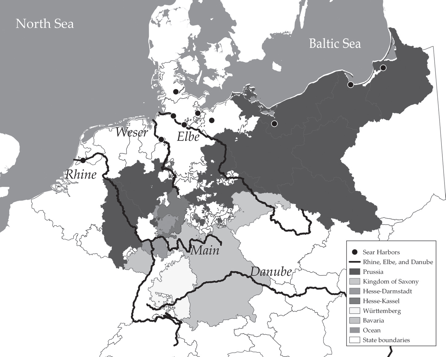
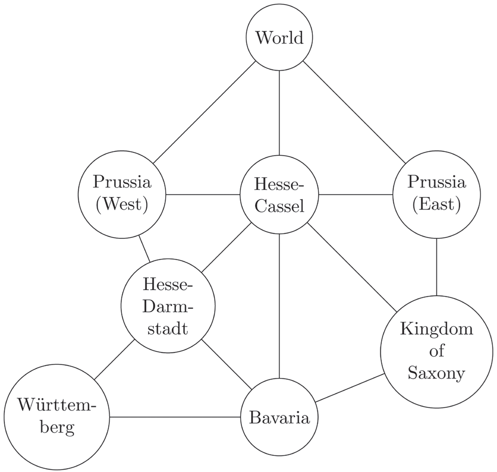
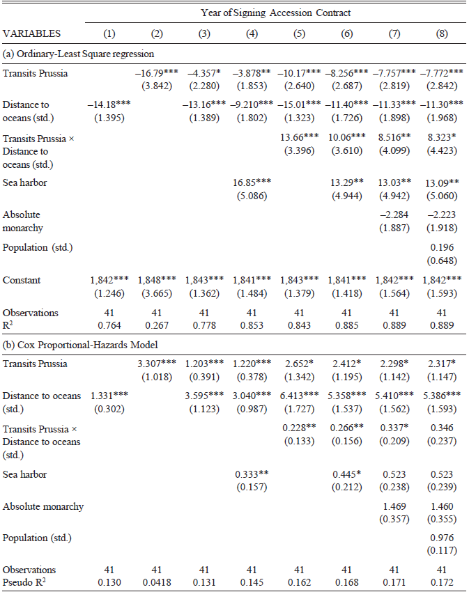
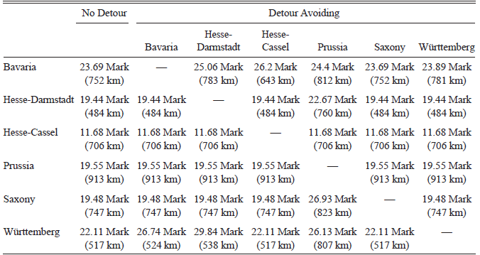
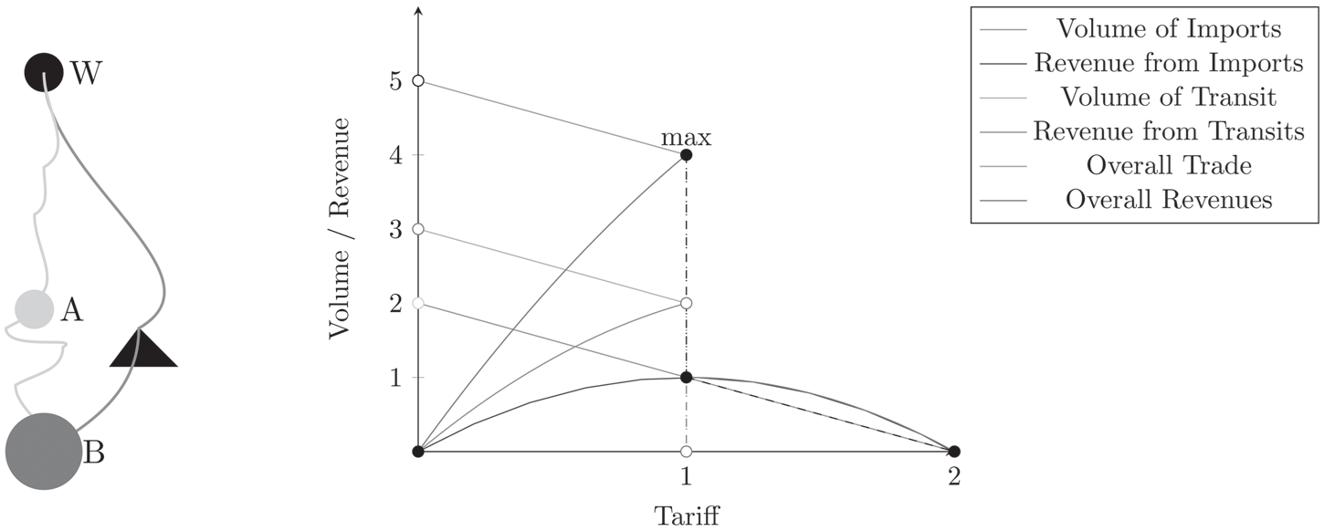
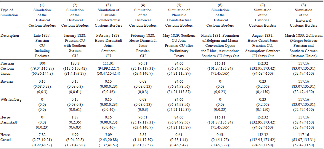
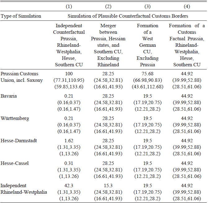


 Open access