2. The wall-wake formulation

While there is no first-principles theory that leads to the turbulent boundary layer velocity profile, the wall-wake formulation introduced by Coles (Reference Coles1956) in his landmark paper provides a very good correlation that accurately reflects the relative balance between viscous and turbulent stresses across most of the layer and can be used to compare flows at different Reynolds numbers. In this formulation, the ${y}$-coordinate and streamwise velocity are normalized using friction variables

(2.1a,b)\begin{equation} {y^+{=} \frac { u_\tau y}{\nu}},\quad {u^+{=} \frac { u}{ u_\tau}}. \end{equation}

The friction Reynolds number, sometimes called the Kármán number and sometimes denoted $\delta ^+$, is the ${y^+}$ coordinate evaluated at ${\delta _h}$,

(2.2)\begin{equation} R_\tau = \frac{u_\tau \delta_h} {\nu}. \end{equation}

Here, $R_\tau$ will be the primary measure of flow Reynolds number in this paper. There is a lower limit, ${R_\tau \approx 100}$, below which wall turbulence cannot be sustained (Schlichting & Gersten Reference Schlichting and Gersten2000, p. 535), whereas the highest Reynolds number laboratory wall flows studied to date can reach ${R_\tau > 500\,000}$ while geophysical flows can reach much higher values. In this range, ${ u^+ }$ at the outer edge of the boundary layer, ${u^+ = u_e / u_\tau }$, varies from a low of approximately $15$ to a high close to $40$ or more.

At the wall, the velocity profile is linear, ${ {\tau _w} / {\rho } = \nu {\partial u} / {\partial y} = \nu { u} / { y }}$, and to a good approximation,

(2.3)\begin{equation} { u^+{=} y^+} \end{equation}

within the so-called viscous sublayer, ${(0 < y^+ \lessapprox 5 ) }$. The Coles wall-wake profile given by

(2.4)\begin{equation} {u^+{=} \frac {1}{\kappa} \ln \left(y^+ \right)} + C + \frac {\varPi \left( x \right)}{\kappa} W \left( \frac{y^+}{R_\tau} \right) \end{equation}

is a good approximation in the range ${( \approx 100 < y^+ < R_\tau )}$. The first two terms of (2.4) comprise the law of the wall introduced by von Kármán (Reference von Kármán1931). Coles (Reference Coles1956) recommends ${ k = 0.41 }$ and ${ C = 5.0 }$. The last term in (2.4) is the law of the wake that Coles determined from a careful study of a variety of flow data for various pressure gradients. The function ${W}$ provides the self-similar shape of the velocity profile in the outer flow, while the function ${\varPi }$ is used to change the amplitude of the outer velocity profile to account for the effect of the pressure gradient. Coles suggested ${W = 2 \sin ^2 (({{\rm \pi} }/{2}) ({y}/{\delta }))}$, where ${{y^+}/{R_\tau } = {y}/{\delta }}$ and ${\delta }$ is the boundary layer thickness, as a good choice for the wake-like shape of the outer velocity profile. For ${d {p_e}/ {\textrm {d}x} = 0}$, Coles used ${\varPi = 0.62}$. The part of the velocity profile that connects the viscous sublayer (2.3) to the beginning of the law of the wall in (2.4) is called the buffer layer.

Missing from the theory at that time, and highly sought after by a number of investigators including Deissler (Reference Deissler1954), van Driest (Reference van Driest1956) and others, was a single formula that could span the entire wall layer connecting the viscous sublayer (2.3) through the buffer layer to the law of the wall. The problem was solved by Spalding (Reference Spalding1961), who came up with the implicit formula,

(2.5)\begin{equation} y^+{=} {u^+} + {\textrm{e}^{-\kappa C} {\left(\textrm{e}^{\kappa {u^+}} - 1 -\kappa {u^+} - \tfrac {1}{2} \left({\kappa {u^+}}\right)^2 - \tfrac {1}{6} \left({\kappa {u^+}}\right)^3 - \tfrac {1}{24} \left({\kappa {u^+}}\right)^4 {\cdots} \right)}} \end{equation}

shown in figure 2. Although somewhat awkward to use, this formula asymptotes to the linear profile at the wall at small ${u^+}$ and approaches the logarithm as the exponential term inside the parentheses dominates the algebraic terms for ${u^+ > 30}$. There are several features of the Coles wall-wake formulation of the velocity profile that can be noted.

1. (i) The velocity derivative has a small discontinuity at the outer edge of the boundary layer owing to the log term that continues to increase with ${y^+}$.

2. (ii) There is a discontinuity at the matching point between the Spalding and Coles profiles where they overlap. At low Reynolds number, the discontinuity becomes quite apparent, requiring additional terms to be included in (2.5).

3. (iii) There is a long running debate as to the validity of the logarithmic dependence of the velocity profile outside the viscous wall layer. The profile (2.4) assumes the log law.

4. (iv) The profile is not connected to any model of the turbulent shear stress.

Figure 2.

Equation (2.5) used by Spalding (Reference Spalding1961) to connect the sublayer to the log region. Dashed curve is ${u^+ = y^+}$. Constants are $\kappa = 0.41$ and $C = 5.0$.

3. The universal velocity profile

Expressing (1.4) in wall normalized coordinates, integrating once and applying the free stream condition, ${\textrm {d} u^+/{\textrm {d}y}^+ = 0}$ at $y^+ = R_\tau$, the result is

(3.1)\begin{equation} {{\tau^+} +\frac {\textrm{d} {u^+}}{\textrm{d}{y^+}} - \left( 1 - \frac {y^+}{R_\tau} \right) = 0}, \end{equation}

where $\tau ^+ = - \overline {u' v'} / (u_\tau )^2$. This equation is identical to the governing stress balance in pipe flow. This fact motivated Subrahmanyam, Cantwell & Alonso (Reference Subrahmanyam, Cantwell and Alonso2021) to approximate velocity profiles in channel flow and the zero pressure gradient boundary layer using the same universal velocity profile used by Cantwell (Reference Cantwell2019) to approximate the Princeton Superpipe (PSP) data (Zagarola Reference Zagarola1996; Zagarola & Smits Reference Zagarola and Smits1998; Jiang, Li & Smits Reference Jiang, Li and Smits2003; McKeon Reference McKeon2003).

In this approach, the shear stress is modelled using classical mixing length theory (von Kármán Reference von Kármán1931; Prandtl Reference Prandtl1934; van Driest Reference van Driest1956),

(3.2)\begin{equation} {\tau^+} = \left( {\lambda \left( y^+ \right)} {\frac{\textrm{d} u^+}{{\textrm{d}y}^+}} \right)^2, \end{equation}

where $\lambda (y^+)$ is the mixing length function. When (3.2) is substituted into (3.1), the result is a quadratic equation for ${\textrm {d} u^+/{\textrm {d}y}^+}$. We use the positive root

(3.3)\begin{equation} \frac{\textrm{d} u^+}{{\textrm{d}y}^+} ={-}\frac{1}{2\lambda(y^+)^2}+ \frac{1}{2\lambda(y^+)^2}\left[1+4\lambda(y^+)^2\left(1-\frac{y^+}{R_\tau}\right)\right]^{1/2}. \end{equation}

Equation (3.3) is integrated from the wall to $y^+$ to obtain the velocity profile in the form of an integral dependent on the non-dimensional mixing length $\lambda (y^+)$ and $R_\tau$,

(3.4)\begin{equation} u^+(y^+) = \int_0^{y^+}\left[-\frac{1}{2\lambda(s)^2}+\frac{1}{2\lambda(s)^2} \left(1+4\lambda(s)^2\left(1-\frac{s}{R_\tau}\right)\right)^{1/2}\right]\textrm{d} s. \end{equation}

At low Reynolds number, (3.4) approaches the laminar channel flow solution

(3.5)\begin{equation} \lim_{R_\tau \to 0} u^+(y^+) = y^+ \left(1- \frac{y^+}{2 R_\tau} \right), \end{equation}

where, in the laminar limit, ${R_\tau = ( 2 {u_e \delta _h} / \nu )^{1/2}}$. The mixing length model introduced by Cantwell (Reference Cantwell2019) to approximate pipe data and used here to approximate channel and boundary layer flow is

(3.6)\begin{equation} \lambda(y^+) = \frac{ky^+\left( 1-\text{e}^{-(y^+{/}a)^m} \right)}{\left(1+\left(\dfrac{y^+}{bR_\tau}\right)^n\right)^{1/n}}. \end{equation}

This model contains five free parameters. The constant ${k}$ is closely related to the Kármán constant and, at high Reynolds number, is essentially equivalent to the $\kappa$ in the wall-wake profile (2.4). The parameter ${a}$ constitutes a wall-damping length scale. The wall model is similar to the exponential decay proposed by van Driest (Reference van Driest1956) except for the exponent ${m}$ that determines the rate of damping. Together, $k$, $a$ and $m$ set the overall size of the wall layer from the viscous sublayer through the buffer layer to the end of the logarithmic region. The outer flow is accounted for in the denominator of (3.6) and includes a length scale ${b}$, which is proportional to the fraction of the wall-bounded layer thickness where wake-like behaviour begins, as well as an exponent ${n}$ that helps shape the outer part of the profile.

The model parameters ${(k, a, m, b, n)}$ for the mixing length model (3.6) are selected by minimizing the total squared error between a given $R_\tau$ data profile and the universal velocity profile (3.4) using the cost function

(3.7)\begin{equation} G = \sum_{i = 1}^N(u^+(k, a, m, b, n, R_\tau, y_i^+)-u_i^+(y_i^+))^2, \end{equation}

where ${N}$ is the number of data points in a given profile. It should be pointed out that the minimization problem solved here is not convex and alternate minima can be found. Further discussion of this issue with an example can be found in the paper by Cantwell (Reference Cantwell2019). At the end of the day, the low ${{u^+}_{rms}}$ error on the order of ${0.2\,\%}$ or less, computed using multiple DNS and experimental data sources, supports the determined parameter values and the efficacy of the universal velocity profile.

The following limits near the wall and approaching the free stream are obtained for $n > 1$:

(3.8)\begin{equation} \left.\begin{gathered} \lim_{y^+ \to 0} \frac {\lambda(y^+)}{ky^+} = (1-\text{e}^{-(y^+{/}a)^m}),\\ \lim_{y^+ \to R_\tau} \frac {\lambda(y^+)}{ky^+} = \frac {1}{\left(1+ \left(\dfrac {1}{b}\right)^n \right)^{1/n}}. \end{gathered}\right\} \end{equation}

Note that if $b< 1$, which is generally the case, and $n$ is large, which can occur in an adverse pressure gradient flow, the normalized mixing length is just ${\lambda (y^+)}/{ky^+} \approx b$ as the free stream is approached. The friction law is generated by evaluating (3.4) at $y^+ = R_\tau$:

(3.9)\begin{equation} \frac{u_e}{u_\tau} = \int_0^{R_\tau}\left[-\frac{1}{2\lambda(s)^2}+ \frac{1}{2\lambda(s)^2}\left(1+4\lambda(s)^2\left(1-\frac{s}{R_\tau}\right)\right)^{1/2}\right]\textrm{d} s. \end{equation}

3.1. The universal velocity profile shape function

Cantwell (Reference Cantwell2019) showed that the universal velocity profile can be expressed in terms of a shape function. Equations (3.4) and (3.6) are repeated here with the full dependence on (${k,a,m,b,n,R_\tau }$) shown:

(3.10)\begin{equation} {u^ + }\left( {k,a,m,b,n,{R_\tau },{y^ + }} \right) = \int_0^{{y^ + }} {\left( { - \frac{1}{{2{\lambda ^2}}} + \frac{1}{{2{\lambda ^2}}}{{\left( {1 + 4{\lambda ^2} \left( {1 - \frac{s}{{{R_\tau }}}} \right)} \right)}^{1/2}}} \right)}\textrm{d} s, \end{equation}

where

(3.11)\begin{equation} \lambda \left( {k,a,m,b,n,{R_\tau },{y^ + }} \right) = \frac{{k{y^ + } \left( {1 - {\exp\left({ - {{\left( {\dfrac{{{y^ + }}}{a}} \right)}^m}}\right)}} \right)}}{{{{\left( {1 + {{\left( {\dfrac{{{y^ + }}}{{b{R_\tau }}}} \right)}^n}} \right)}^{{1}/{n}}}}}. \end{equation}

Equations (3.10) and (3.11) admit a scaling that can be used to reduce the number of independent model parameters by one and determine the high Reynolds number limiting behaviour of a wall-bounded layer. Use the group, ${u / u_0 \to ku / u_0}$, ${y^+ \to ky^+}$ and ${R_ \tau \to kR_ \tau }$ to define a modified wall-wake mixing length function by multiplying and dividing various terms in (3.11) by ${k}$:

(3.12)\begin{align} & \lambda \left( {k,a,m,b,n,{R_\tau },{y^ + }} \right) = \frac{{k{y^ + }\left( {1 - {\exp\left({ - {{\left( {\dfrac{{{y^ + }}}{a}} \right)}^m}}\right)}} \right)}}{{{{\left( {1 + {{\left( {\dfrac{{{y^ + }}}{{b{R_\tau }}}} \right)}^n}} \right)}^{{1}/{n}}}}} \nonumber\\ &\quad =\frac{{k{y^ + }\left( {1 - {\exp\left({ - {{\left( {\dfrac{{k{y^ + }}}{{ka}}} \right)}^m}}\right)}} \right)}}{{{{\left( {1 + {{\left( {\dfrac{{k{y^ + }}}{{b\left( {k{R_\tau }} \right)}}} \right)}^n}} \right)}^{{1}/{n}}}}} = \tilde \lambda \left( {ka,m,b,n,k{R_\tau },k{y^ + }} \right). \end{align}

In the reduced space, ${k}$ and ${a}$ are not independent parameters. Multiply both sides of (3.10) by ${k}$ and insert the modified mixing length function (3.12). Choose the integration variable, ${\alpha = ky^+}$,

(3.13)\begin{equation} k{u^ + } = \int_0^{k{y^ + }} {\left( { - \frac{1}{{2{{\tilde \lambda }^2}}} + \frac{1}{{2{{\tilde \lambda }^2}}}{{\left( {1 + 4{{\tilde \lambda }^2} \left( {1 - \frac{\alpha }{{k{R_\tau }}}} \right)} \right)}^{1/2}}} \right)} \textrm{d}\alpha. \end{equation}

Equation (3.13) is a ${k}$-independent model velocity profile, $k u^+$, with four model parameters, (${ka,m,b,n}$) in a wall-bounded layer at the scaled friction Reynolds number, ${k R_\tau }$. Now, define the shape function:

(3.14)\begin{align} & \varPhi \left( {ka,b,m,n,k{R_\tau },k{y^ + }} \right) \nonumber\\ &\quad =\int_0^{k{y^ + }} {\left( { - \frac{1}{{2{{\tilde \lambda }^2}}} + \frac{1}{{2{{\tilde \lambda }^2}}}{{\left( {1 + 4{{\tilde \lambda }^2} \left( {1 - \frac{\alpha }{{k{R_\tau }}}} \right)} \right)}^{1/2}}} \right)} \textrm{d}\alpha - \ln\left( {k{y^ + }} \right). \end{align}

Note that ${k{y^ + } = (y/\delta _h )k{R_\tau }}$. The shape function, (3.14), has the property that, for fixed ${( {y/\delta _h} )}$, it approaches a constant value as ${k{R_\tau } \to \infty }$. Importantly, the limit is approached quite rapidly, and for ${k{R_\tau } > 2000 }$, the limit is fully established over almost the entire thickness of the wall-bounded layer except very close to the wall:

(3.15)\begin{equation} \phi ( ka, m, b, n, y/ \delta_h) = \lim_{kR_\tau > 2000} \varPhi ( ka, m, b, n, k R_\tau, k y^+). \end{equation}

In the same limit, the velocity and friction laws, (3.4) and (3.9), become

(3.16)\begin{equation} \lim_{kR_\tau > 2000} \frac{u}{u_\tau} = \frac{1}{k} \ln (k y^+) + \frac{1}{k} \phi \left( ka, m, b, n, \frac{y} {\delta_h}\right) \end{equation}

and

(3.17)\begin{equation} \lim_{kR_\tau > 2000} \frac{u_e}{u_\tau} = \frac{1}{k} \ln (k R_\tau) + \frac{1}{k} \phi ( ka, m, b, n, 1). \end{equation}

There are two issues that need to be addressed when integrating the universal velocity profile: one is the removable singularity near $y^+ = 0$, which can be addressed straightforwardly (Kollmann Reference Kollmann2020), the other is the very small value of $\textrm {d} u^+ / {\textrm {d}y}^+$ in the wake region. Figure 7(a) gives some idea of the difficulty, although $\textrm {d} u^+ / {\textrm {d}y}^+$ is easily integrated for the values of $R_\tau$ shown there. However, once $R_\tau$ exceeds $10^5$ or so, the integration can be quite slow. Fortunately this problem is essentially solved through the use of the shape function. In practice, the shape function is determined by simply evaluating $\varPhi$ by (3.14) at any $R_\tau > 2000/k$, to produce $\phi$ by (3.15) (Cantwell Reference Cantwell2019, Reference Cantwell2021). Any velocity profile with $R_\tau > 2000/k$ can then be generated by integrating $\textrm {d} u^+ / {\textrm {d}y}^+$ (3.4) only over the lowest few percent of the wall flow. The rest of the profile out to $y^+ = R_\tau$ is generated using (3.16). If $\varPhi$ is evaluated at say $R_\tau = 10^5$, then the overlap region is at $y/\delta _h \approx 0.01$. This makes it possible to quickly generate the velocity profile at essentially any Reynolds number. This topic is discussed further in § 6, where the shape function for adverse pressure gradient boundary layers is discussed.

This formulation of the velocity profile has several useful features.

1. (i) The profile (3.4) with the mixing length model (3.6) is uniformly valid over ${ 0 \leq y \leq \delta _h }$ and $0 \leq R_\tau < \infty$. There is no need for a buffer layer function and there is no discontinuity in the velocity derivative at the outer edge of a boundary layer. At low Reynolds number, the velocity profile reverts to the laminar pipe/channel solution.

2. (ii) There is no presumption of logarithmic dependence of the velocity profile outside the viscous wall layer and so the profile can better approximate low-Reynolds-number wall-bounded flows.

3. (iii) The mixing length model (3.6) can be used in computational fluid dynamics (CFD) based on the full RANS equations.

4. (iv) Optimal values of the model parameters ${(k, a, m, b, n)}$ are determined through a procedure designed to minimize the error over the whole profile.

5. (v) Using optimal values of the model parameters ${(k, a, m, b, n)}$ enables subtle Reynolds number and geometry effects to be detected and compared.

6. (vi) Mean values of the model parameters can provide a good approximation to the velocity profile for a given geometry over a wide range of Reynolds numbers.

7. (vii) The accuracy of the fit to the velocity profile is such that extrapolation to Reynolds numbers beyond the range of available data can be used to explore the structure of the velocity profile in the limit of infinite Reynolds number (Pullin, Inoue & Saito Reference Pullin, Inoue and Saito2013; Cantwell Reference Cantwell2019; Kollmann Reference Kollmann2020; Cantwell Reference Cantwell2021).

3.2. Landmarks of the universal velocity profile, the friction law

Mean parameter values, $(\bar {k},\bar {a},\bar {m},\bar {b},\bar {n})$ for smooth wall pipe, channel and zero-pressure-gradient boundary layer flow are shown in table 1. The averages for $k$, interpreted as the Kármán constant, are close to traditional values. The pipe flow average of $k=0.4092$ is in agreement with the conclusion of $\kappa = 0.41$ by Nagib & Chauhan (Reference Nagib and Chauhan2008) after they re-examined the Princeton Superpipe data, but the channel and boundary layer averages in table 1 are considerably higher than their value of $\kappa = 0.384$ for the boundary layer and $\kappa \approx 0.37$ for channel flow. The boundary layer value is also larger than $\kappa = 0.37$ found by Inoue & Pullin (Reference Inoue and Pullin2011) using a high-Reynolds-number LES simulation. As yet, there is really no explanation for these differences although it is worth noting that optimum values of $(k, a, m, b, n)$ are determined through a procedure designed to minimize the error over the whole profile and the achieved errors are small.

Table 1.

Mean model parameters for canonical wall flows. Pipe flow means are obtained by averaging optimal parameters for PSP cases 6 to 26 in table 1 of Cantwell (Reference Cantwell2019). Means for channel flow and the boundary layer are generated by averaging optimal parameters from tables 3 and 4.

To examine the structure of the universal velocity profile, multiply the velocity gradient (3.3) by ${y^+}$ to generate the log-law indicator function $y^+ \textrm {d} u^+/{\textrm {d}y}^+$. The basic idea is to reveal a flat region that would identify where the velocity profile is logarithmic. In practice, a minimum in the log indicator function will always occur but an extended flat region will not unless the Reynolds number is large enough to ensure a certain degree of scale separation between the viscous wall layer and outer wake flow. If a log region can be identified, the value of the log indicator function at the minimum is the inverse of the parameter ${k}$ which can be identified with the Kármán constant, ${1/k = 1/\kappa }$, that appears in the wall-wake profile (2.4). In figure 3, the log indicator functions for pipe, channel and zero pressure gradient boundary layer flow are plotted at a value of $R_\tau = 10^6$ chosen to insure well-separated inner and outer length scales. Mean parameter values from table 1 are used to generate the curves. The close-up view in figure 3(b) reveals details of the intermediate region.

Figure 3.

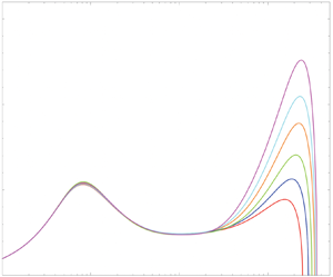
(a,b) Log indicator functions for pipe (red), channel (blue) and boundary layer flow (magenta) at $R_\tau = 10^6$ using mean parameter values from table 1. Coordinate values of extrema I, II, III and IV are provided in table 2. (c) Normalized length scale function for channel flow at 12 values of $R_\tau$ differing by factors of 2 beginning at $R_\tau = 500$. Dashed line is the free stream limit in (3.8). (d) Friction law, (3.9), including the laminar range using parameter values from table 1.

The structure of the log indicator function presents an opportunity to adopt a consistent convention for defining various regions of the flow. Several extrema are identified in figures 3(a) and 3(b) using the notation in Cantwell (Reference Cantwell2019). These can be thought of as landmarks in the velocity profile.

1. (i) The outer edge of the viscous sublayer is defined here as the peak at I.

2. (ii) Every profile has a maximum in the middle of the wake region designated as III.

3. (iii) There is a minimum between I and III at all Reynolds numbers but the outer edge of the buffer layer and beginning of the intermediate (logarithmic) region, defined as the minimum at II, only begins to be localized near $y^+ \approx 60 - 140$, for $R_\tau \gtrapprox 12\,000$. The viscous wall layer ends at the outer edge of the buffer layer; at $y^+ = (y^+)_{II}$ when the minimum at II is present.

4. (iv) If $R_\tau$ is greater than approximately $40\,000$, then a second minimum begins to appear at IV. The second minimum unambiguously marks the end of the log region and beginning of the wake region. When the minimum at IV appears, there is also a broad region where $\lambda \approx k y^+$, which indicates complete scale separation between the inner and outer flows. See the mixing length function for channel flow in figure 3(c). The wall layer ends at the outer edge of the log layer; at $y^+ = (y^+)_{IV}$ when the minimum at IV is present.

5. (v) The maximum at V that develops for $R_\tau \gtrapprox 40\,000$ designates the broad middle of the intermediate region where the velocity profile is precisely logarithmic and outer and inner length scales are well separated.

The coordinates of the extrema (other than V) for the three flows are provided in table 2. The positions of extrema I and II generally follow the trend indicated by the values of the near-wall parameters $(k, a, m)$. Table 2 shows the values of $(y^+)_{II}$ for pipe, channel and the boundary layer. This point is at the end of the buffer layer and is determined by the parameters $k$, $a$ and $m$ in table 2. The smallest $a$ and largest $m$ produce the smallest $(y^+)_{II}$ (pipe flow) whereas the largest $a$ and smallest $m$ produce the largest $(y^+)_{II}$ (boundary layer) with more than a factor of two between the two flows. The point IV is important because it defines the outer boundary of the wall layer that could potentially be modelled in an LES computation using wall functions. Changing $R_\tau$ over several orders of magnitude from $10^5$ to $10^{10}$ has no significant effect on the values in table 2.

Table 2.

Coordinates of the extrema in figure 3 in wall or outer coordinates. Descriptors of the velocity profile: viscous sublayer $0< y^+<(y^+)_{I}$; viscous wall layer $0< y^+<(y^+)_{II}$; wall layer (includes log region) $0< y^+<(y^+)_{IV}$; wake layer $(y^+)_{IV}< y^+< R_\tau$.

Below $R_\tau \gtrapprox 40\,000$, the log indicator function has only one minimum between I and III. The data exhibit a logarithmic section of the velocity profile at this minimum and, at first sight, this would seem to indicate significant separation between the wall and wake regions. This issue can be examined further by looking at the normalized length scale function $\lambda (y^+) / {k y^+}$ shown in figure 3(c) using the mean parameter values for channel flow. This figure shows the dependence of the mixing length on Reynolds number with a flat section of increasing length with increasing Reynolds number. This is the crucial feature of the mixing length model that enables it to approximate the Reynolds number dependence of wall-bounded flows with empirical constants that depend, at most, weakly on the Reynolds number. Significant scale separation begins to be present only when there is a clearly identifiable region where $\lambda (y^+) / {k y^+} \approx 1$. Looking at figure 3(c), this appears to be the case beginning with the sixth curve from the left at $R_\tau = 16\,000$.

3.2.1. The friction law

Figure 3(d) shows the friction law for the three canonical flows using the averaged parameters in table 1. Above $R_\tau \approx 2000/k$, $u_e/u_\tau$ closely follows (3.17) and the additive constant is

(3.18)\begin{equation} C = (\ln(k)+\phi(ka, m, b, n, 1))/k. \end{equation}

For the pipe, channel and boundary layer, the values of C are $6.219$, $5.628$ and $8.900$, respectively. Below $R_\tau \approx 2000/k$, (3.9) must be used to determine $u_e / u_\tau$.

It should be noted that the curves in figure 3(d) are generated by a single set of parameters for each flow. There is a subtle point to be made when the friction law is determined from more than one dataset, which is generally the case. Because the channel and boundary layer data in the present paper comprise a relatively limited number of cases over a narrow range of Reynolds numbers, pipe flow, where the averages in table 1 come from profiles 6 to 26 of the PSP experiments covering two orders of magnitude in the Reynolds number, will be used to illustrate the point. The pipe friction law presented in figure 3(d) is $u_e / u_\tau =(1/0.4092)\ln (R_\tau )+6.219$, where $k = 0.4092$ in table 1 is the average over PSP profiles 6 to 26. This can be compared to figure 23(a) in Cantwell (Reference Cantwell2019), where the friction law is given as $u_e / u_\tau =(1/0.4309)\ln (R_\tau )+7.5115$. Why the difference? The answer has to do with the fact that over profiles 6 to 26, there is a small Reynolds number variation; $k$ and $a$ both increase slightly with increasing Reynolds number. 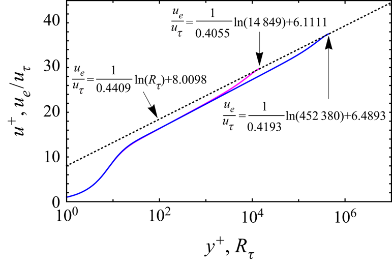When profiles 6 to 26 are all used to generate the friction law for pipe flow, the values of $k$ and $C$ that fit the friction law are quite different from the $k$ and $C$ that describe any one profile and they are not averages. The issue is illustrated using the construction in figure 4, where two PSP velocity profiles widely separated in $R_\tau$ are plotted on the same axes as the friction law that they generate. The value of $k$ for the friction law (dashed line) is considerably larger than either value of $k$ for each individual velocity profile. If both profiles had the same $k$, there would be no difference. Something similar can be said for $C$, each profile has a different $C$ (also a consequence of the weak Reynolds number dependence of the optimal parameters) but the friction law generated by the aggregate of all profiles only has one $C$ and it is considerably larger than the $C$ for either profile.

Figure 4.

Two PSP velocity profiles at $R_\tau = 14\,849$ (magenta) and $R_\tau = 452\,380$ (blue). The values of $k$ and $C$ for each profile are indicated and the arrows point to $u_e / u_\tau$ for each profile. The dashed line is the friction law generated when the two end points are joined by a straight line.

4. Channel flow

Simulation data for channel flow were taken from multiple sources: Lee & Moser (Reference Lee and Moser2015) ($R_\tau = 550$, 1001, 1995, 5186), Bernardini, Pirozzoli & Orlandi (Reference Bernardini, Pirozzoli and Orlandi2014) ($R_\tau = 4079$), Lozano-Durán & Jiménez (Reference Lozano-Durán and Jiménez2014) ($R_\tau = 4179$) and Yamamoto & Tsuji (Reference Yamamoto and Tsuji2018) ($R_\tau = 8016$). All cases exhibited a small degree of uncertainty in the form of non-zero mean spanwise velocity in wall units of $O(10^{-3})$ with peaks of approximately $|w^+| \approx 0.007$ for the largest deviation from zero. Turbulence is inherently three-dimensional and spanwise fluctuations will not average to zero in the finite time of even a very well-converged, long time-averaged numerical solution. The spanwise velocity tends to be largest in the wake region where bulk mixing with long time scales occurs, but is also evident in all regions. As an example, the spanwise velocity distribution for $R_\tau =5186$ from Lee & Moser (Reference Lee and Moser2015) is shown in figure 5(a). According to figure 5(a), the variation in the mean spanwise velocity, $w^+$, is roughly 10 % of the error in the fit of the universal velocity profile to the streamwise velocity data. One could reasonably view the peak in $|w^+|$ as providing a rough lower bound of the error in the fit that can be achieved with the universal velocity profile.

Figure 5.

(a) Spanwise velocity, $w^+$, for $R_\tau =5186$ channel flow DNS from Lee & Moser (Reference Lee and Moser2015). (b) Channel flow DNS velocity profiles from Lee & Moser (Reference Lee and Moser2015), Lozano-Durán & Jiménez (Reference Lozano-Durán and Jiménez2014), Bernardini et al. (Reference Bernardini, Pirozzoli and Orlandi2014) and Yamamoto & Tsuji (Reference Yamamoto and Tsuji2018) at $R_\tau =550$ (dark blue); 1001 (green); 1995 (dark red); 4079 (yellow); 4179 (purple); 5186 (light blue); 8016 (light red). Profiles are separated vertically by 10 units.

The channel data are shown in figure 5(b). The minimization procedure leads to the optimal channel flow parameter values shown in table 3. The fit using optimal parameter values for each case is shown in figure 6(a). The data exhibit an increasingly well-defined wake region as $R_\tau$ increases. For $R_\tau =4079$ and above, the region between the buffer and wake regions is increasingly logarithmic. The largest errors in the profile, on the order of 0.1 in units of $u^+$, tend to occur near the wall for $10 < y^+ < 20$ and are associated with a slight overestimation of the velocity gradient as the flow transitions from the viscous sublayer to the buffer layer. Even so, the fit is generally excellent for each case.

Table 3.

Reynolds number, optimal model parameters and root-mean-square (r.m.s.) error for channel flow datasets. Second column is extrapolation of $u/u_\tau$ data to channel centreline. Third column is $u_e/u_\tau$ calculated using the universal velocity profile (uvp).

Figure 6.

Channel flow velocity profiles from Lee & Moser (Reference Lee and Moser2015), Lozano-Durán & Jiménez (Reference Lozano-Durán and Jiménez2014), Bernardini et al. (Reference Bernardini, Pirozzoli and Orlandi2014) and Yamamoto & Tsuji (Reference Yamamoto and Tsuji2018) overlaid on the universal velocity profile with (a) optimal parameters from table 3 and (b) average parameter values from table 1 for $(\bar {k},\bar {a},\bar {m},\bar {b},\bar {n})$ at $R_\tau =550$ (dark blue), 1001 (green), 1995 (dark red), 4079 (yellow), 4179 (purple), 5186 (light blue), 8016 (light red). Profiles are separated vertically by 10 units.

To illustrate the sensitivity of the channel profiles to the relatively small variations in parameter values shown in table 3 compared with the averages in table 1, the profile comparison in figure 6(a) is repeated in figure 6(b) but with average values of the parameters used for each profile. The largest error still tends to occur in the region $10 < y^+ < 20$ and is of the same order as when optimal parameters are used. In addition, the error in the logarithmic region for the largest $R_\tau$ cases is slightly more pronounced. Still, the universal profile gives excellent agreement for all regions and all profiles.

Note that in table 3, and the other tables in the paper, the number of significant figures retained in the parameter values is intended to allow an interested reader to be able to reproduce the results shown here with the same degree of error. The $u_e/u_\tau$ values in table 3 column 3 are calculated using the universal profile with the optimal parameters for each case. While the parameters do not vary significantly with $R_\tau$, there is a distinct decrease in $k$ and $a$ between cases at $R_\tau =1995$ and below, and cases at $R_\tau =4079$ and above. In pipe flow, a similar drop in ${k}$ and ${a}$ occurs between $R_\tau =2345$ and $R_\tau =4124$. In both geometries, the drop appears to be associated with increased mixing by the underlying turbulence. The optimal value of ${b}$ for the pipe tends to be closer to ${0.3}$ compared with ${0.4}$ for the channel. Both exponents ${m}$ and ${n}$ are slightly larger in the case of pipe flow compared with channel flow. Given the equivalence between the governing equations in pipe and channel flow, these differences can be viewed as purely arising from geometrical effects.

4.1. Channel flow velocity gradient and turbulence properties determined from the universal velocity profile

With the mean velocity and a model for the turbulent shear stress known, a variety of channel flow properties can be studied. In figure 7(a), the velocity gradient, (3.3), is plotted in log–log coordinates clearly delineating the linear part of the viscous sublayer ${y^+ \lessapprox 5}$ and showing the position of the wake region as $R_\tau$ increases. It is the integral of this function that generates the universal velocity profile. As the free stream is approached, the velocity gradient drops rapidly to zero as the limiting behaviour,

(4.1)\begin{equation} \lim_{y^+ \to R_\tau} \frac{\textrm{d} u^+}{\textrm{d}y^+} = \left(1- \frac{y^+}{ R_\tau} \right), \end{equation}

is reached. In figure 7(b), by comparing the log indicator functions of the universal velocity profile at the various Reynolds numbers of the data, only a single minimum appears and an identifiable flat region just begins to appear at $R_\tau =8016$. Collapse of the five highest Reynolds number velocity profiles in the viscous wall layer below ${y^+ \approx 80}$ is essentially perfect indicating a degree of insensitivity to small variations in the wall parameters ${(k, a, m)}$.

Figure 7.

(a) Channel flow velocity gradient and (b) log indicator function at ${R_\tau }$ values for channel flow DNS cases in table 3.

In figure 8, the log indicator function from the universal profile is compared with the ${R_\tau = 5186}$ data of Lee & Moser (Reference Lee and Moser2015) and the ${R_\tau = 8016}$ data of Yamamoto & Tsuji (Reference Yamamoto and Tsuji2018). The agreement between the data and the universal profile is generally very good although the profile does not accurately match the dip in the DNS velocity gradient that occurs between the buffer layer and the logarithmic region at approximately $y^+ = 60$ for ${R_\tau = 5186}$ with a clear flat section at ${y^+ = 500}$. This dip would coincide with the minimum II defined in § 3.2 except that the Reynolds number is too low to make that correspondence exact given the low degree of scale separation. The agreement between the universal profile and the ${R_\tau = 8016}$ data in figure 8(b) with a dip at ${y^+ \approx 70}$ and a flat section at ${y^+ = 800}$ is somewhat better. However, the universal velocity profile does not generate a localized minimum at II unless $R_\tau > 12\,000$, so there is still an unexplained discrepancy. Optimal values of $k$ for the two cases ($0.3950$ and $0.3964$) are slightly larger than the values of the Kármán constant ($\kappa = 0.384$ and $0.387$) reported by Lee & Moser (Reference Lee and Moser2015) and Yamamoto & Tsuji (Reference Yamamoto and Tsuji2018). In both comparisons, the peak of the universal profile near the wall at I occurs at a slightly lower ${y+}$ and has a slightly larger maximum value than either DNS dataset. The agreement in figure 8 in the outer wake region is nearly perfect in both cases.

Figure 8.

Channel flow DNS data from Lee & Moser (Reference Lee and Moser2015) and Yamamoto & Tsuji (Reference Yamamoto and Tsuji2018) compared with the universal velocity profile. (a) $R_\tau =5186$ and (b) $R_\tau =8016$.

4.1.1. Channel flow turbulent shear stress and kinetic energy (TKE) production

An expression for the Reynolds shear stress profile can be generated from (3.1), (3.3) and (3.6) as

(4.2)\begin{align} \tau^+{=} 1-\frac{y^+}{R_\tau} - \frac{\textrm{d} u^+}{{\textrm{d}y}^+} = 1-\frac{y^+}{R_\tau}+ \frac{1}{2\lambda(y^+)^2}-\frac{1}{2\lambda(y^+)^2}\left[1+4\lambda(y^+)^2 \left(1-\frac{y^+}{R_\tau}\right)\right]^{1/2}. \end{align}

Equation (4.2) is plotted in figure 9(a) for the various DNS values of $R_\tau$. Near-wall damping drives $\tau ^+$ to zero to a high order in ${y^+}$ in the viscous wall layer. The $y^+$ position of the maximum in $\tau ^+$ occurs roughly in the middle of the the log layer and increases with ${( R_\tau / k)^{1/2}}$. Above the log layer, the viscous term in (3.1) becomes negligible and the balance of $\tau ^+$ against the pressure gradient accounts for almost all the momentum transport.

Figure 9.

Channel shear stress and TKE production generated using the universal velocity profile in (4.2). (a) Channel $\tau ^+$ profiles and (b) channel flow $P^+$ profiles.

The turbulent kinetic energy (TKE) production $P = - (\overline {u'v'}) \,\textrm {d} u /{\textrm {d}y}$ is obtained from the product of Reynolds shear stress and the velocity gradient:

(4.3)\begin{equation} P^+{=} \tau^+\frac{\textrm{d} u^+}{{\textrm{d}y}^+} = \left(1-\frac{y^+}{R_\tau}\right) \frac{\textrm{d} u^+}{{\textrm{d}y}^+}-\left(\frac{\textrm{d} u^+}{{\textrm{d}y}^+}\right)^2, \end{equation}

where $P^+ = P \nu / u_\tau ^4$. Using (4.3), it can be easily shown that at high Reynolds number, the maximum in TKE production occurs where ${\textrm {d} u^+/{\textrm {d}y}^+ = 1/2}$ and the value of the peak is ${P^+ = 1/4}$ (Sreenivasan Reference Sreenivasan1989; Chen, Hussain & She Reference Chen, Hussain and She2018; Cantwell Reference Cantwell2019; Chen & Sreenivasan Reference Chen and Sreenivasan2021). Equation (4.3) is plotted in figure 9(b) for the various cases listed in table 3. The position of the peak above the wall is at $y^+ \approx 12$, near the lower edge of the buffer layer just above ${(y^+)}_{I}$, close to the value found in pipe flow. The overlap of all cases except ${R_\tau = 550}$ is nearly perfect.

The cumulative TKE production between the wall and channel midline is

(4.4)\begin{equation} \overline{P^+} (y^+) = \frac {1}{R_\tau} \int_0^{y^+} \left( \tau^+\frac{\textrm{d} u^+}{\textrm{d} s} \right) \textrm{d} s. \end{equation}

Using the channel flow average parameter values in table 1, the mean TKE production averaged across the channel is

(4.5)\begin{equation} \overline{P^+} (R_\tau) = \frac {1}{R_\tau} \left( 2.458 \ln (R_\tau) - 6.421 \right), \end{equation}

which is very close to the comparable expression in pipe flow (Cantwell Reference Cantwell2019, (7.19)). The cumulative TKE production normalized by the total is shown in figure 10, where the distribution across the whole layer is shown along with a close-up near the wall. The outer edge of the log region, $(y/ \delta _h)_{IV} = 0.01181$ from table 2, is indicated by a vertical dashed line. Note that the minimum IV is only present if $R_\tau > 40\,000$ and so the dashed line only crosses the six contours corresponding to $R_\tau = 10^{5}$ to $R_\tau = 10^{10}$.

Figure 10.

Cumulative channel flow TKE production versus $y^+$ generated using mean parameters from table 1. Contours vary from $R_\tau = 10^2$ to $R_\tau = 10^{10}$ by factors of 10. The outer edge of the log region and beginning of the wake is identified by the vertical dashed line at $(y/\delta _h)_{IV} = 0.01181$. The extremum IV does not occur below $R_\tau = 40\,000$.

Although the highest rate of TKE production occurs very close to the wall below $(y^+)_{II}$, a substantial fraction of the total TKE generated is produced in the wake layer and even at the highest Reynolds number, more than 20 % of the total TKE is generated in the wake region. At moderate Reynolds numbers of the order of $R_\tau = 10^{5}$, the fraction is closer to 50 %.

5. Zero pressure gradient boundary layer

In the boundary layer case, the flow variation in the streamwise direction does not vanish and the boundary layer equation (1.2a,b) does not simplify to one that is easily integrated. Although the universal velocity profile is not a solution of this equation, we will push on and see if (3.4) and (3.6) can be used to approximate turbulent boundary simulation and experimental data. In figure 1, the boundary layer thickness is denoted $\delta _h$ and an explanation was promised. The thickness $\delta _h$ will be called the boundary layer equivalent channel half-height. The concept is introduced and explained in detail by Cantwell (Reference Cantwell2021). See pp. 12–13 and figures 17–23 in that paper.

The universal velocity profile is fundamentally a pipe/channel profile with a well-defined outer edge where $u/u_e = 1$ and ${\partial u} / {\partial y} = 0$ at the channel midpoint $y/ \delta _h = 1$. These properties of the profile are only approached asymptotically in the boundary layer and an outer length scale that falls short of these conditions must be defined. The most common choice is the boundary layer thickness corresponding to $u_e/U = 0.99$, where $U$ is the free stream velocity reported with the data.

The boundary layer equivalent channel half-height, $\delta _h$, is defined as the thickness that minimizes the error between the universal velocity profile and a given dataset. This provides a well-defined, practically useful, alternative to an arbitrary choice of $u_e/U$.

Figure 11 shows how changing the choice of $u_e / U$ changes the optimal fit to the Sillero, Jiménez & Moser (Reference Sillero, Jiménez and Moser2013) data. The minimum error is achieved for $u_e / U = 0.994$ (Cantwell Reference Cantwell2021, figure 17). If $u_e / U > 0.994$, the error increases fairly rapidly because several data points at the edge of the boundary layer are included where the velocity is virtually constant. The optimization procedure will try to fit these points and this will tend to degrade the accuracy over the whole profile causing the error to increase. If $u_e / U < 0.994$, the data are cut off short of the boundary layer edge, and the derivative condition, ${\partial u} / {\partial y} = 0$ at $y/ \delta _h = 1$, is applied where the derivative is not quite zero. This produces a more gentle increase in the error. Relevant data for each curve in figure 11 is provided in the figure caption. The value $R_\tau = 1989$ reported with the Sillero et al. (Reference Sillero, Jiménez and Moser2013) data corresponds to $u_e / U = 0.990$. The value of $R_\tau$ corresponding to $u_e / U = 0.994$ is $R_\tau = 2088$ and this is the number provided in table 4 along with optimal parameter values.

Figure 11.

Optimal fit of the universal velocity profile (blue curves) to the data of Sillero et al. (Reference Sillero, Jiménez and Moser2013) (open circles) for three choices of $u_e / U$. Curves and data are shifted vertically by 4 units for viewing. Upper curve $u_e / U = 0.999$, $R_\tau = 2471$, $(k, a, m, b, n) = (0.4201, 25.1850, 1.1650, 0.1719, 2.2415)$, $u^+_{rms} = 0.2074$; middle curve $u_e / U = 0.994$, $R_\tau = 2088$, $(k, a, m, b, n) = (0.4289, 25.9290, 1.1480, 0.1696, 2.2516)$, $u^+_{rms} = 0.0314$; lower curve $u_e / U = 0.980$, $R_\tau = 1834$, $(k, a, m, b, n) = (0.4338, 25.8676, 1.1746, 0.1733, 2.3251)$, $u^+_{rms} = 0.0805$.

Table 4.

Reynolds number, optimal model parameters and r.m.s. error for turbulent boundary layer datasets. Second column is $u / u_\tau$ data interpolated at the boundary layer edge, $y=\delta _h, y^+ = R_\tau$. Third column is $u_e/u_\tau$ calculated using the universal velocity profile (uvp) at $y^+ = R_\tau$.

The value of $u_e / U$ that minimizes the error is a unique property of a given profile dataset. In principle, it can change from one profile to another depending on the precise details on how the data were measured and reported. Looking at tables 4 and 5, there appears to be no evidence that the optimal value of $u_e / U$ depends on $R_\tau$. It does appear that, as a rule, $u_e / U = 0.995$ is a good choice, generally better than $u_e / U = 0.990$. This discussion will be continued in § 6, where the determination of $\delta _h$ is described for the adverse pressure gradient data of Perry & Marusic (Reference Perry and Marusic1995a,Reference Perry and Marusicb).

Table 5.

Run data, Reynolds number, optimal model parameters and r.m.s. error for adverse pressure gradient boundary layer datasets from Perry & Marusic (Reference Perry and Marusic1995b). Initial free stream values are $u_\infty = 10$ and $u_\infty = 30$ m s$^{-1}$. Column seven is $u / u_\tau$ data interpolated at boundary layer edge, $y=\delta _h, y^+ = R_\tau$, as shown in figure 19.

The boundary layer simulation data are taken from: Simens et al. (Reference Simens, Jiménez, Hoyas and Mizuno2009), Borrell, Sillero & Jiménez (Reference Borrell, Sillero and Jiménez2013), Sillero et al. (Reference Sillero, Jiménez and Moser2013) (${R_\tau = 1343, 1475, 1616, 1779, 1962, 2088}$) and Ramis & Schlatter (Reference Ramis and Schlatter2014) (${R_\tau = 2571}$). The experimental data at ($R_\tau = 2109, 4374, 9090, 17\,207$) are from Baidya et al. (Reference Baidya, Phillip, Hutchins, Monty and Marusic2017, Reference Baidya, Phillip, Hutchins, Monty and Marusic2021). The length scale for evaluating $R_\tau$ for all cases is ${\delta _h}$ chosen through the error minimization scheme just described. The same cost function, (3.7), is used to identify model parameters ${(k, a, m, b, n)}$ that minimize the total squared error. The resulting parameter values are presented in table 4. The $R_\tau$ values for the Baidya et al. (Reference Baidya, Phillip, Hutchins, Monty and Marusic2017, Reference Baidya, Phillip, Hutchins, Monty and Marusic2021) data listed in table 4 are between 5 % and 15 % lower than the reported values. Baidya et al. (Reference Baidya, Phillip, Hutchins, Monty and Marusic2017) calculated $R_\tau$ using the boundary layer thickness determined from a fit of the data to the composite profile of Monkewitz, Chauhan & Nagib (Reference Monkewitz, Chauhan and Nagib2007) and Chauhan, Monkewitz & Nagib (Reference Chauhan, Monkewitz and Nagib2009) which extends beyond $\delta _h = \delta _{0.996}$ used here.

The simulation data with comparison to the universal velocity profile using optimal parameters for each profile are shown in figure 12(a). The parameters, $(k, a, m)$, lead to a viscous wall layer that is approximately a third thicker than in channel flow. The outer flow parameters, $(b, n)$, indicate a smaller outer length scale when compared with channel flow with a more pronounced wake-like shape, as can be seen in figures 12(a) and 12(b). The nearly discontinuous decrease in the parameters $k$ and $a$ between ${R_\tau = 2000}$ and ${R_\tau = 4000}$ that occurs in pipe and channel flow is not seen in the boundary layer datasets. Instead, there is a small increase between the highly resolved LES at $R_\tau = 2571$ and the experiments at $R_\tau = 2109$ and $R_\tau = 4374$ followed by a decrease in ${k}$ between ${R_\tau = 4374}$ and ${R_\tau = 9090}$.

Figure 12.

Turbulent boundary layer DNS data from Simens et al. (Reference Simens, Jiménez, Hoyas and Mizuno2009), Borrell et al. (Reference Borrell, Sillero and Jiménez2013), Sillero et al. (Reference Sillero, Jiménez and Moser2013) and Ramis & Schlatter (Reference Ramis and Schlatter2014) at $R_\tau =1343$ (dark blue), 1475 (green), 1616 (dark red), 1779 (yellow), 1962 (purple), 2088 (light blue) and 2571 (light red) compared with the universal velocity profile using (a) optimal parameters from table 4, (b) average parameters from 1. Profiles are separated vertically by 10 units.

The largest error between the DNS data and the universal profile is, again, of the order of 0.1 in units of $u^+$ and occurs in the region $10 < y^+ < 20$ in the buffer layer. Nevertheless, the fit for this region is still quite good and, in fact, the universal velocity profile accurately fits the entire dataset very well. The small variation of the parameters over all boundary layer datasets supports the applicability of the universal velocity profile, (3.4) and (3.6), to the boundary layer geometry. Average parameter values from table 1 are used in figure 12(b) and, again, the optimal and average fits are very close.

The velocity gradient and log indicator function for each boundary layer simulation case are shown in figure 13. The wake section of the boundary layer profile is much more pronounced with a larger variation in the gradient compared with channel flow and pipe flow leading to a substantially larger second peak at $(y^+ / \delta _h)_{III}$ in the wake region of the log indicator function.

Figure 13.

Velocity derivative and log indicator function using boundary layer data with average parameters. The $R_\tau$ legend shows values reported with the data for $u_e / U = 0.99$. The $R_\tau$ values in table 4 were used to make the curves. (a) Velocity gradient and (b) log-law indicator function.

5.1. The universal profile in the context of the boundary layer equations

The zero pressure gradient form of (1.2a,b) is

(5.1a,b)\begin{equation} \frac{\partial}{\partial x}(u u) + \frac{\partial}{\partial y}(u v) = \frac{\partial \tau}{\partial y} + \nu\frac{\partial^2 u}{\partial y^2},\quad {\frac{\partial u}{\partial x} + \frac{\partial v}{\partial y} = 0}. \end{equation}

The fit of the log indicator function, derived from the universal velocity profile, to the Ramis & Schlatter (Reference Ramis and Schlatter2014) ${R_\tau = 2479}$ data (${R_\tau = 2571}$ in table 4) is shown in figure 14(a). The fit is at least comparable to and perhaps somewhat better than it was in the channel flow examples, and the r.m.s. errors presented in table 4 are comparable to or lower than in the channel flow case. This is a little surprising and raises obvious questions. Why does the universal profile derived for pipe flow work so well in the boundary layer and what is the role of the convective terms in (5.1a,b)?

Figure 14.

Boundary layer log-law indicator function for $R_\tau =2479$ Ramis & Schlatter (Reference Ramis and Schlatter2014) data (${R_\tau = 2571}$ in table 4) compared with the universal profile and turbulent shear stress data compared with the shear stress generated using the universal velocity profile in (5.6). The dashed line in panel (b) is the pipe/channel shear stress generated directly from (3.2) and (3.6). (a) Log indicator function and (b) turbulent shear stress.

To examine these questions, we recast (5.1a,b) in wall units. The Kármán integral form of the boundary layer equation with zero pressure gradient is

(5.2)\begin{equation} \frac{\textrm{d} \theta}{\textrm{d}x} = \frac {C_f}{2} = \left(\frac{u_\tau}{u_e}\right)^2, \end{equation}

where ${\theta }$ is the boundary layer momentum thickness. The momentum thickness Reynolds number can be written in terms of wall units as

(5.3)\begin{equation} {R_\theta}=\frac {u_e \theta}{\nu} = \int_0^{R_\tau} u^+ \left(1 - \frac {u_\tau}{u_e} {u^+} \right) {\textrm{d}y}^+. \end{equation}

Equation (5.2) can be rearranged to read

(5.4)\begin{equation} \frac{\textrm{d} R_\theta}{\textrm{d} R_\tau} = \frac {\left(\dfrac{u_\tau}{u_e}\right)^2}{\dfrac{\textrm{d} \left( R_\tau \right)}{\textrm{d} R_x}}. \end{equation}

Differentiate (5.3) with respect to ${R_\tau }$:

(5.5)\begin{equation} \frac{\textrm{d} R_\theta} {\textrm{d} R_\tau} = \frac{\partial}{\partial R_\tau} {\int_0^{R_\tau} u^+ {\textrm{d}y}^+} - \left(\frac {u_\tau} {u_e} \right) \frac{\partial}{\partial R_\tau} {\int_0^{R_\tau} {u^+}^2 {\textrm{d}y}^+} - \frac{\partial}{\partial R_\tau} \left(\frac {u_\tau} {u_e} \right) {\int_0^{R_\tau} {u^+}^2 {\textrm{d}y}^+}. \end{equation}

Now express (5.1a,b) in wall units and integrate with respect to $y^+$. Use (5.4) and (5.5) to replace differentiation in ${R_x}$ with differentiation in ${R_\tau }$ and solve for the Reynolds stress term in (5.1a,b):

(5.6)\begin{align} \tau^+{=} 1-\frac{\partial u^+}{\partial y^+} - \left( \frac { u^+ \displaystyle\frac{\partial}{\partial R_\tau} {\int_0^{y^+} u^+ {\textrm{d}y}^+} - \frac{\partial}{\partial R_\tau} {\int_0^{y^+} {{u^+}^2} {\textrm{d}y}^+} - \left(\frac {u_e} {u_\tau} \right) \frac{\textrm{d}}{\textrm{d} R_\tau} \left(\frac {u_\tau} {u_e} \right) {\int_0^{y^+} {u^+}^2 {\textrm{d}y}^+}} {\displaystyle \left(\frac {u_e} {u_\tau} \right) \frac{\textrm{d}}{\textrm{d} R_\tau} {\int_0^{R_\tau} u^+ {\textrm{d}y}^+} - \frac{\textrm{d}}{\textrm{d} R_\tau} {\int_0^{R_\tau} {u^+}^2 {\textrm{d}y}^+} - \left(\frac {u_e} {u_\tau} \right) \frac{\textrm{d}}{\textrm{d} R_\tau} \left(\frac {u_\tau} {u_e} \right) {\int_0^{R_\tau} {u^+}^2 {\textrm{d}y}^+}} \right). \end{align}

When (5.6) is evaluated, the derivative $\textrm {d}({u_e / u_\tau })/{\textrm {d} R_\tau }$ that appears in the third term is generated by differentiating the friction law equation (3.9) with respect to $R_\tau$.

What about the Reynolds shear stress model (3.2) and (3.6) that is used in the solution of the channel flow equation (3.1) to generate the universal velocity profile? If this were plotted against (5.6), it would agree closely in the wall layer but would not agree in the wake region where it must give the linear stress profile across the channel implied by (3.1). To a degree, (3.2) and (3.6) are disconnected from the true physical Reynolds shear stress in the boundary layer given by (5.6). The model is simply part of the universal velocity profile used in (5.6). Figure 15 shows the turbulent stress generated from (5.6) using average ZPG boundary layer parameter values from table 1. The shape of the ${\tau ^+}$ profile in figure 15 has the expected smooth transition to zero that must occur at the outer edge of the boundary layer.

Figure 15.

Reynolds shear stress using average parameter values for the universal profile in (5.6) for ${(R_\tau = 500,1000, 2000, 4000, 8000)}$. (a) Linear coordinates and (b) log–linear coordinates.

Figure 14(b) compares the Reynolds shear stress data from the Ramis & Schlatter (Reference Ramis and Schlatter2014) DNS case with the shear stress generated from the universal velocity profile in (5.6) with the optimal parameters listed in table 4. The agreement between the two sets of data is very good. The maximum in the DNS data is ${{\tau ^+}_{max} = 0.97199}$ at ${y^+ = 164.52}$. The maximum generated by the universal velocity profile is ${{\tau ^+}_{max} = 0.97068}$ and is slightly closer to the wall at ${y^+ = 134.61}$. The main disagreement between the two datasets occurs in the wake region where the DNS is several percent higher than the universal velocity profile. At ${y^+ = 2571}$, the ${\tau ^+}$ generated by the universal profile goes to zero, while the DNS data are at approximately ${0.07}$. The dashed line in figure 14(b) shows the pipe/channel shear stress generated directly from (3.2) and (3.6). The difference between the two is why (5.6) has to be used to generate the Reynolds stress for the boundary layer. The difference between the dashed line and the actual boundary layer shear stress indicates stronger mixing and is consistent with the much fuller wake region of the boundary layer compared with the pipe and channel flow.

Figure 16 shows the velocity data measured by Baidya et al. (Reference Baidya, Phillip, Hutchins, Monty and Marusic2017, Reference Baidya, Phillip, Hutchins, Monty and Marusic2021) overlaid on the universal velocity profile with optimal parameters listed in table 4. Minimum error occurs using $u_e / U = 0.996$ for all four cases. The highest Reynolds number cases, $R_\tau =9090$ and $R_\tau =17\,207$, exhibit approximately 3 to 4 times the error compared with the DNS cases although the error appears to be comparable to or smaller than the experimental uncertainty inferred indirectly from figure 2 of Baidya et al. (Reference Baidya, Phillip, Hutchins, Monty and Marusic2017). The two lower Reynolds number cases, $R_\tau = 2109$ and $R_\tau = 4374$, have the highest values of $k$ and $a$ among the cases. Overall, the agreement between the data and the universal profile is very good.

Figure 16.

Velocity data from Baidya et al. (Reference Baidya, Phillip, Hutchins, Monty and Marusic2021) overlaid on the universal velocity profile with optimal parameters from table 4. Profiles are separated vertically by 10 units. (a) Linear coordinates and (b) log–linear coordinates.

Figure 17 shows the Reynolds shear stress data measured by Baidya et al. (Reference Baidya, Phillip, Hutchins, Monty and Marusic2017, Reference Baidya, Phillip, Hutchins, Monty and Marusic2021) overlaid on the shear stress generated using the universal velocity profile in (5.6) with optimal parameters from table 1. The agreement with data is generally excellent away from the wall in the outer part of the boundary layer. Below $y^+ = 150$, the data collapse but drop off more rapidly than the stress generated by the universal velocity profile. Some discussion of this issue can be found in Baidya et al. (Reference Baidya, Phillip, Hutchins, Monty and Marusic2017) with reference to figure 2(c) in their paper where they note common discrepancies up to 15 % between measured Reynolds stresses and stress distributions generated from DNS or the composite mean velocity formulation noted earlier (Monkewitz et al. Reference Monkewitz, Chauhan and Nagib2007; Chauhan et al. Reference Chauhan, Monkewitz and Nagib2009). The fact is that spatial resolution limitations make measurements of the Reynolds stress very near the wall extremely difficult.

Figure 17.

Reynolds shear stress data from Baidya et al. (Reference Baidya, Phillip, Hutchins, Monty and Marusic2021) compared with the Reynolds shear stress determined from the universal velocity profile inserted into (5.6) using optimal parameters from table 4. (a) Linear coordinates and (b) log–linear coordinates.

Figure 18 shows the TKE production and log indicator functions generated using the universal velocity profile with optimal parameters from table 1 for the Baidya et al. (Reference Baidya, Phillip, Hutchins, Monty and Marusic2017, Reference Baidya, Phillip, Hutchins, Monty and Marusic2021) data. Despite some variation in the wall parameters for this data, the TKE profiles in figure 18(a) collapse very well. Although the higher Reynolds number cases have a fairly well-defined nearly flat region between approximately $y_+ = 110$ and $y_+ = 500$, the Reynolds number is still too low to generate the well-defined minima at II and IV described in figure 3.

Figure 18.

TKE production and log indicator function generated from the universal velocity profile using optimal parameters from the Baidya et al. (Reference Baidya, Phillip, Hutchins, Monty and Marusic2021) data in table 4. (a) Turbulent kinetic energy production and (b) log indicator function.

6. The adverse pressure gradient boundary layer

The universal profile is used to approximate the Perry & Marusic (Reference Perry and Marusic1995a,Reference Perry and Marusicb) adverse pressure gradient data for the two upstream velocity cases, $u_\infty =10$ and $u_\infty =30$ m s$^{-1}$. Perry & Marusic (Reference Perry and Marusic1995b) used dynamically calibrated X-hot-wires to measure mean velocity and turbulence profiles in a decelerating flow. A flying hot-wire apparatus was used to translate the probe in the streamwise direction adding a bias velocity to insure that the measured velocity vector did not fall outside the cone of sensitivity of the X-wire. This is particularly important near the wall where instantaneous velocity fluctuations can occasionally exceed the mean velocity. A similar approach was used by Cantwell & Coles (Reference Cantwell and Coles1983) to measure the flow in the highly turbulent near wake of a circular cylinder.

As noted in § 5, defining the thickness of the boundary layer tends to be a somewhat arbitrary process. Both Vinuesa et al. (Reference Vinuesa, Bobke, Örlu and Schlatter2016) and Griffin, Fu & Moin (Reference Griffin, Fu and Moin2021) discuss several approaches to this issue in the context of pressure gradient boundary layers.

In the present study, the same method described in § 5 for the zero pressure gradient boundary layer was used to determine $\delta _h$ for the adverse pressure gradient cases. The procedure for one of the profiles is illustrated in figure 19. An interpolation function is used to approximate the profile data for a selected value of $u_e / U$, where $U$ is the free stream value reported with the data. The interpolated point at $\delta _h$ is then included with the data used to determine optimal parameters for that $u_e / U$. Data above this point are excluded from the optimization procedure. The process is repeated at several values of $u_e / U$ and the minimum error is determined. It turns out that for every Perry & Marusic (Reference Perry and Marusic1995b) profile, the minimum error occurs at $\delta _h$ corresponding to $u_e / U = 0.998$. The relatively large value of $u_e / U$ compared with the zero pressure gradient cases seems to arise from the rather rapid, channel-flow-like approach to $\partial u/ \partial y = 0$ at the edge of the adverse pressure gradient boundary layer. This is the $\delta _h$ used to evaluate $R_\tau$ as well as the values of $u_e / u_\tau$ presented in table 5. These values are generally somewhat smaller than those reported by Perry & Marusic (Reference Perry and Marusic1995b) who defined their thickness, $\delta _c$, in terms of the Rotta–Clauser thickness based on an integral of the velocity defect law (Rotta Reference Rotta1953; Clauser Reference Clauser1954). The differences in $R_\tau$ and $u_e / u_\tau$ are shown graphically in figure 20 for the two datasets.

Figure 19.

Dimensional velocity profile from the Perry & Marusic (Reference Perry and Marusic1995b), $u_\infty = 10$ m s$^{-1}$ case at $x=2.240$ m. Open red circles are the data, the solid black curve is an interpolation function. The filled magenta circle is the thickness reported with the Perry & Marusic (Reference Perry and Marusic1995b) data. The filled green circle is the thickness at $u_e =0.998 U$ and is included with the data in the optimization procedure. (a) The $u_\infty = 10$ m s$^{-1}$ profile at 2.240 m and (b) close-up of panel (a) at the boundary layer edge.

Figure 20.

Comparison between $R_\tau$ computed from the $\delta _{998}$ thickness (filled circles) and the $R_\tau$ values reported by Perry & Marusic (Reference Perry and Marusic1995b) (open circles). (a) The $u_\infty = 10$ m s$^{-1}$ case and (b) the $u_\infty = 30$ m s$^{-1}$ case.

Perry & Marusic (Reference Perry and Marusic1995b) express the strength of the pressure gradient in terms of the Clauser parameter $\beta = (\delta _1 / \tau _w) (\textrm {d} p / {\textrm {d}x})$, where $\delta _1$ is the displacement thickness. Values of $\beta$ are included in table 5. The Clauser parameter varies from 0 to approximately 7 for both flow velocity cases corresponding to a boundary layer that is strongly decelerating but not close to separation. For a rough perspective, the fractional velocity change calculated in (6.2) is approximately what would occur on a NACA 0012 airfoil at high Reynolds number and zero angle of attack between the point of minimum pressure and the trailing edge.

Figures 21 and 22 show the comparison between the data and the universal velocity profile using the optimal parameter values ${(k,a,m,b,n)}$ listed in table 5. Errors in fitting the lower Reynolds number, $u_\infty = 10$ m s$^{-1}$, case are almost twice as large as in the high-Reynolds-number case. Moreover, there is more scatter between the two thicknesses depicted in figure 20. Nevertheless, the agreement is generally very good, well within the experimental uncertainty inferred from Perry & Marusic (Reference Perry and Marusic1995b), and comparable to the error in the Baidya et al. (Reference Baidya, Phillip, Hutchins, Monty and Marusic2017, Reference Baidya, Phillip, Hutchins, Monty and Marusic2021) ZPG data in table 4.

Figure 21.

Comparison between the universal velocity profile and the $u_\infty = 10$ m s$^{-1}$ adverse pressure gradient data of Perry & Marusic (Reference Perry and Marusic1995b) (open red circles). (a) Linear coordinates and (b) log coordinates.

Figure 22.

Comparison between the universal velocity profile and the $u_\infty = 30$ m s$^{-1}$ adverse pressure gradient data of Perry & Marusic (Reference Perry and Marusic1995b) (open red circles). (a) Linear coordinates and (b) log coordinates.

The near wall parameters in table 5 are shown in figures 23(a) to 23(d). They show very little variation with streamwise distance indicating, importantly, that the near wall velocity profile expressed in wall units is insensitive to the adverse pressure gradient aside from the direct effect of the pressure gradient on the wall shear stress itself. The wall parameters do show a small decrease with the factor of 2 increase in $R_\tau$ between the two cases. In contrast, the outer flow parameters in figures 24(a) and 24(b) vary quite strongly. The wake component of the velocity profile begins closer and closer to the wall as the flow decelerates. This is reflected in decreasing values of the optimal value of the outer flow length scale, $b$, with streamwise distance along the plate. The exponent $n$ increases with streamwise distance and it should be noted that for values of $n$ above approximately $5.0$ or so, the velocity profile becomes quite insensitive to $n$.

Figure 23.

Optimal near wall parameters of the universal profile, ($k$, $a$, $m$), evaluated on the data of Perry & Marusic (Reference Perry and Marusic1995b). Open circles correspond to the $u_\infty = 10$ m s$^{-1}$ case, filled circles correspond to the $u_\infty = 30$ m s$^{-1}$ case. Horizontal coordinate is the streamwise position of the corresponding velocity profile. (a) Parameter $k$; (b) parameter $a$; (c) parameter product $ka$; and (d) parameter $m$.

Figure 24.

Optimal wake parameters of the universal velocity profile, $b$ and $n$, evaluated on the data of Perry & Marusic (Reference Perry and Marusic1995b). Open circles correspond to the $u_\infty = 10$ m s$^{-1}$ case, filled circles correspond to the $u_\infty = 30$ m s$^{-1}$ case. Horizontal coordinate is the streamwise position of the corresponding velocity profile. (a) Parameter $b$ and (b) parameter $n$.

To examine the effect that small $b$ and large $n$ have on the velocity profile shape, the first and last velocity profiles of the $u_\infty = 10$ m s$^{-1}$ case and the $u_\infty = 30$ m s$^{-1}$ case are presented in figure 25 along with their shape functions in figure 26 and mixing length functions in figure 27. As noted earlier, the shape function becomes independent of $R_\tau$ when $R_\tau >2000/k$. Neither of the Perry & Marusic (Reference Perry and Marusic1995b) cases meet this criterion although the 30 m s$^{-1}$ case is close. And so, with reference to (3.14) and (3.15), figure 26 is plotted in terms of $\varPhi$ instead of $\phi$. In the construction of figure 26, the relation $ky^+ = k R_\tau y/\delta _h$ has been used in (3.14). The shape function depicts the wake portion of the velocity profile scaled by $k$. Note that the shape function is larger in the lower Reynolds number case in figure 26(a) and that in the two cases, the point where the shape functions at $x = 3.08$ and $x = 1.20$ m depart from one another is very close to the same point of departure of the two velocity profiles in figure 25 and both are close to the values of $b$. At the end of the adverse pressure gradient region, the wake component of the velocity profile is much more pronounced than at the beginning and the velocity profile over the mid-region of the boundary layer is nearly linear, reminiscent of a Couette flow profile. Referring back to the mixing length model (3.6) and the limits in (3.8), it can be seen in figure 27 that, in the presence of an adverse pressure gradient leading to small $b$ and large $n$ at the farthest downstream station, the mixing length $\lambda$ tends toward a constant over most of the wake layer,

(6.1)\begin{equation} \lambda(y^+) \approx bkR_\tau. \end{equation}

Figure 25.

Velocity data from Perry & Marusic (Reference Perry and Marusic1995b) (open red circles) at $x = 1.2$ and $x = 3.08$ m compared with the universal profile at the first and last stations in $x$: (a) $u_\infty = 10$ m s$^{-1}$ and (b) $u_\infty = 30$ m s$^{-1}$.

Figure 26.

Boundary layer shape function from the universal profile at $x = 1.2$ and $x = 3.08$ m: (a) $u_\infty = 10$ m s$^{-1}$ and (b) $u_\infty = 30$ m s$^{-1}$.

Figure 27.

Mixing length model (3.6), for the universal profile at $x = 1.2$ and $x = 3.08$ m: (a) $u_\infty = 10$ m s$^{-1}$ and (b) $u_\infty = 30$ m s$^{-1}$.

The relative velocity change in both Perry & Marusic (Reference Perry and Marusic1995b) datasets is approximately the same.

(6.2)\begin{equation} \left.\begin{gathered} \left( \frac{U_{3.080\,\textrm{m}} - U_{1.200\,\textrm{m}}}{U_{1.200\,\textrm{m}}} \right)_{10\,\textrm{m}\,\textrm{s}^{{-}1}} = \frac{7.911748 - 10.38199}{10.38199} ={-}0.237935,\\ \left( \frac{U_{3.080\,\textrm{m}} - U_{1.200\,\textrm{m}}}{U_{1.200\,\textrm{m}}} \right)_{30\,\textrm{m}\,\textrm{s}^{{-}1}} = \frac{22.95415 - 30.76513}{30.76513} ={-}0.253891. \end{gathered}\right\} \end{equation}

Furthermore, the fairly significant effect of Reynolds number on the shape functions depicted in figure 26 does not involve significant changes in $b$ or $n$ in figure 24. These features of the data support the conclusion that the main effect of the Reynolds number between the two adverse pressure gradient datasets is captured by the inherent Reynolds number dependence of the universal velocity profile.

Plots of the log-indicator function for the $u_\infty = 10$ and $u_\infty = 30$ m s$^{-1}$ velocity profiles are shown in figure 28. The collapse of the profiles near the wall is nearly perfect and consistent with all the other wall flows discussed. Not surprisingly, the most dramatic difference occurs in the wake region where the peak reaches three times the zero pressure gradient value of approximately $5$. The other distinctive feature of these plots is the consistency in the point where the curves depart from one another at the inner boundary of the wake layer; approximately $y^+ = 60$ in the $u_\infty = 10$ m s$^{-1}$ case and $y^+ = 220$ in the $u_\infty = 30$ m s$^{-1}$ case.

Figure 28.

Log-indicator function generated by the universal velocity profile at each $x$ position using optimal parameters for $u_\infty = 10$ and $u_\infty = 30$ m s$^{-1}$: (a) $u_\infty = 10$ m s$^{-1}$ and (b) $u_\infty = 30$ m s$^{-1}$.