





1. Introduction
Melting of ice bodies or solid particles plays a central role in diverse natural and industrial contexts, ranging from oceanography and planetary science to astrophysics and metallurgy (Davis Reference Davis2001). When external flows are present, whether driven by buoyancy or imposed by forced convection, the surrounding temperature field is altered, producing complex body interface morphologies during melting. These evolving interfaces, in turn, modify the flow by acting as moving boundaries. Understanding this coupled fluid–thermal–interface dynamics is essential for predicting iceberg ablation (Cenedese & Straneo Reference Cenedese and Straneo2023), interpreting the formation of magma oceans (Ulvrová et al. Reference Ulvrová, Labrosse, Coltice, Råback and Tackley2012), reconstructing the thermal histories of icy moons (Gastine & Favier Reference Gastine and Favier2025) and controlling solidification defects in metallurgical processes (Shevchenko et al. Reference Shevchenko, Boden, Gerbeth and Eckert2013).
Overthe past two decades, significant progress has been achieved through laboratory experiments, numerical simulations and theoretical analyses. Much of this progress has relied on simplified model systems. A canonical configuration is Rayleigh–Bénard convection (Lohse & Shishkina Reference Lohse and Shishkina2024), where buoyancy drives turbulent motion that interacts with a melting boundary. The closed geometry and high experimental controllability of this set-up make it an attractive framework for studying melting dynamics (Du, Calzavarini & Sun Reference Du, Calzavarini and Sun2024). Foundational contributions include the experiments by Davis, Müller & Dietsche (Reference Davis, Müller and Dietsche1984) and the simulations by Ulvrová et al. (Reference Ulvrová, Labrosse, Coltice, Råback and Tackley2012), Rabbanipour Esfahani et al. (Reference Rabbanipour Esfahani, Hirata, Berti and Calzavarini2018) and Favier, Purseed & Duchemin (Reference Favier, Purseed and Duchemin2019), which revealed unsteady processes such as convective roll mergers and shell-like melting fronts. These studies also proposed scaling laws for interface evolution and melting rates derived from energy balances. Recent extensions of this framework have incorporated additional physical complexities to better approximate geophysical and engineering scenarios. Examples include the anomalous temperature dependence of water density (Wang et al. Reference Wang, Calzavarini, Sun and Toschi2021a ), ambient shear and turbulence (Couston et al. Reference Couston, Hester, Favier, Taylor, Holland and Jenkins2021; Ravichandran, Toppaladoddi & Wettlaufer Reference Ravichandran, Toppaladoddi and Wettlaufer2022; Yang et al. Reference Yang, Howland, Liu, Verzicco and Lohse2023) and double-diffusive effects in solute-laden systems (Xue, Zhang & Ni Reference Xue, Zhang and Ni2024; Guo & Yang Reference Guo and Yang2025). Such modifications have been shown to exert profound influence on interface morphology and melting rates. For instance, Couston et al. (Reference Couston, Hester, Favier, Taylor, Holland and Jenkins2021) demonstrated that turbulent kinetic energy promotes ripple- and scallop-like structures, while Xue et al. (Reference Xue, Zhang and Ni2024) showed that solute concentration gradients can suppress convective transport, thereby inhibiting morphological pattern formation.
In contrast to Rayleigh–Bénard convection, where melting typically occurs at extended boundaries, a complementary class of problems involves melting bodies of finite extent immersed in open flows. This scenario is particularly relevant to iceberg ablation, which exhibits nonlinear sensitivity to ocean currents (FitzMaurice, Cenedese & Straneo Reference FitzMaurice, Cenedese and Straneo2017). Both the magnitude and shear of surface flows strongly control melting rates and interface morphology (Wagner et al. Reference Wagner, Wadhams, Bates, Elosegui, Stern, Vella, Abrahamsen, Crawford and Nicholls2014; FitzMaurice & Stern Reference FitzMaurice and Stern2018). A simplified yet fundamental model considers a stationary ice body in a uniform current, isolating the role of forced convection from buoyancy-driven drift. Pioneering experiments by Hao & Tao (Reference Hao and Tao2001, Reference Hao and Tao2002) on ice spheres in horizontal flows demonstrated that melting rates increase with both fluid velocity and temperature, and that enhanced wake circulation downstream promotes heat transfer, leading to flattened rear surfaces. Orientation-dependent melting rates have since been widely reported. For example, Hester et al. (Reference Hester, McConnochie, Cenedese, Couston and Vasil2021) showed that vertical faces melt faster than horizontal ones in saline flows. More recently, numerical studies by Yang et al. (Reference Yang, Howland, Liu, Verzicco and Lohse2024a ,Reference Yang, van den Ham, Verzicco, Lohse and Huisman b ) and Xu et al. (Reference Xu, Yang, Verzicco and Lohse2025) established that melting rate depends non-monotonically on body aspect ratio, and developed scaling arguments based on distinct conductive and convective contributions. Despite such complexities, experiments and simulations consistently indicate that the upstream face of melting spheres converges to a self-similar profile (Hao & Tao Reference Hao and Tao2001; Yang et al. Reference Yang, Howland, Liu, Verzicco and Lohse2024a ). Comparable shape evolution has also been reported for eroding or dissolving bodies in unidirectional flows (Ristroph et al. Reference Ristroph, Moore, Childress, Shelley and Zhang2012; Moore et al. Reference Moore, Ristroph, Childress, Zhang and Shelley2013; Huang et al. Reference Huang, Jinzi, M.Nicholas and Ristroph2015, Reference Huang, Tong, Shelley and Ristroph2020), where boundary-layer models accurately capture the emergence of self-similar forms. In turbulent environments, generated for instance by meltwater plumes or subglacial discharge, local flow intensification can further accelerate melting rates (Machicoane, Bonaventure & Volk Reference Machicoane, Bonaventure and Volk2013; McCutchan, Meyer & Johnson Reference McCutchan, Meyer and Johnson2024).
While recent work has advanced the quantification of melting rates and global heat transfer efficiency, comparatively little is known about the associated flow dynamics and hydrodynamic loading. In particular, detailed information on the time evolution of wake structures and force histories for melting bodies is scarce. Moreover, most numerical studies have focused on two-dimensional (2-D) geometries such as circles and ellipses (Yang et al. Reference Yang, Howland, Liu, Verzicco and Lohse2024a
,Reference Yang, van den Ham, Verzicco, Lohse and Huisman
b
), leaving three-dimensional (3-D) effects largely unexplored. This gap is significant because the wake behind a non-melted rigid sphere undergoes well-documented bifurcations: a steady axisymmetric-to-planar transition near $\textit{Re}\approx 212$
(Magnaudet & Mougin Reference Magnaudet and Mougin2007), a Hopf bifurcation to periodic vortex shedding near
$\textit{Re}\approx 212$
(Magnaudet & Mougin Reference Magnaudet and Mougin2007), a Hopf bifurcation to periodic vortex shedding near $\textit{Re}\approx 273$
(Fabre, Auguste & Magnaudet Reference Fabre, Auguste and Magnaudet2008) and ultimately a chaotic 3-D state at higher Reynolds numbers (Ern et al. Reference Ern, Risso, Fabre and Magnaudet2012). How these canonical wake transitions are altered when the sphere is melting and its shape evolves remains poorly understood.
$\textit{Re}\approx 273$
(Fabre, Auguste & Magnaudet Reference Fabre, Auguste and Magnaudet2008) and ultimately a chaotic 3-D state at higher Reynolds numbers (Ern et al. Reference Ern, Risso, Fabre and Magnaudet2012). How these canonical wake transitions are altered when the sphere is melting and its shape evolves remains poorly understood.
Motivated by this question, we present 3-D direct numerical simulations of a melting sphere across the initial Reynolds number range $25 \leqslant \textit{Re}_0 \leqslant 1000$
. A sharp-interface method (Xue et al. Reference Xue, Zhao, Ni and Zhang2023, Reference Xue, Zhang and Ni2024), based on a hybrid volume-of-fluid (VOF) and embedded-boundary (EB) method, is employed to resolve the flow and temperature fields in both liquid and solid phases separately, with interfacial conditions enforced explicitly. We consider a pure substance without solutal effects to focus on thermal melting under forced and mixed convection. The paper is organised as follows. The governing model and numerical approach are introduced in § 2. Section 3 examines flow patterns and interfacial morphologies across parameter regimes when buoyancy force is excluded. Section 4 quantifies melting rates, comparing with classical scaling laws and incorporating shape effects to improve prediction. Section 5 analyses the time-dependent hydrodynamic forces and torques, while § 6 explores the influence of buoyancy-driven convection. Concluding remarks and perspectives are given in § 7.
$25 \leqslant \textit{Re}_0 \leqslant 1000$
. A sharp-interface method (Xue et al. Reference Xue, Zhao, Ni and Zhang2023, Reference Xue, Zhang and Ni2024), based on a hybrid volume-of-fluid (VOF) and embedded-boundary (EB) method, is employed to resolve the flow and temperature fields in both liquid and solid phases separately, with interfacial conditions enforced explicitly. We consider a pure substance without solutal effects to focus on thermal melting under forced and mixed convection. The paper is organised as follows. The governing model and numerical approach are introduced in § 2. Section 3 examines flow patterns and interfacial morphologies across parameter regimes when buoyancy force is excluded. Section 4 quantifies melting rates, comparing with classical scaling laws and incorporating shape effects to improve prediction. Section 5 analyses the time-dependent hydrodynamic forces and torques, while § 6 explores the influence of buoyancy-driven convection. Concluding remarks and perspectives are given in § 7.
2. Problem statement, governing equations and numerical method
The configuration considered is shown in figure 1. An initially spherical solid particle ( $\varOmega ^s$
) of diameter
$\varOmega ^s$
) of diameter $D_0$
and uniform temperature
$D_0$
and uniform temperature $T=T_0$
is fixed at the origin
$T=T_0$
is fixed at the origin $\boldsymbol{x} = (x,y,z)= (0,0,0)$
and immersed in its warmer liquid phase (
$\boldsymbol{x} = (x,y,z)= (0,0,0)$
and immersed in its warmer liquid phase ( $\varOmega ^\ell$
), representing the translational motion of a melting sphere. The liquid is incompressible and quiescent at
$\varOmega ^\ell$
), representing the translational motion of a melting sphere. The liquid is incompressible and quiescent at $t=0$
. A Cartesian coordinate system is adopted with the
$t=0$
. A Cartesian coordinate system is adopted with the $x$
axis aligned with the streamwise direction. At the inflow boundary (
$x$
axis aligned with the streamwise direction. At the inflow boundary ( $x=-4D_0$
), uniform velocity
$x=-4D_0$
), uniform velocity $\boldsymbol{U} = (U_\infty , 0, 0)$
and temperature
$\boldsymbol{U} = (U_\infty , 0, 0)$
and temperature $T = T_\infty \gt T_0$
are prescribed, while an outflow condition is applied at
$T = T_\infty \gt T_0$
are prescribed, while an outflow condition is applied at $x=16D_0$
. Lateral boundaries (
$x=16D_0$
. Lateral boundaries ( $y=\pm 10D_0$
,
$y=\pm 10D_0$
, $z=\pm 10D_0$
) are treated as adiabatic and free-slip.
$z=\pm 10D_0$
) are treated as adiabatic and free-slip.
Schematic of the numerical set-up (not to scale). A solid sphere composed of a pure substance with initial diameter $D_0$
, denoted by
$D_0$
, denoted by $\varOmega ^s$
, with uniform initial temperature
$\varOmega ^s$
, with uniform initial temperature $T = T_0$
, is immersed in its warmer liquid phase,
$T = T_0$
, is immersed in its warmer liquid phase, $\varOmega ^\ell$
, driven by an incoming flow. At the inflow boundary, a uniform velocity
$\varOmega ^\ell$
, driven by an incoming flow. At the inflow boundary, a uniform velocity $\boldsymbol{U} = (U_\infty , 0, 0)$
and temperature
$\boldsymbol{U} = (U_\infty , 0, 0)$
and temperature $T = T_\infty \gt T_0$
are imposed.
$T = T_\infty \gt T_0$
are imposed.

Using $D_0$
,
$D_0$
, $U_\infty$
and
$U_\infty$
and $\Delta T=T_\infty -T_0$
as characteristic length, velocity and temperature scales, the governing equations for the liquid phase are
$\Delta T=T_\infty -T_0$
as characteristic length, velocity and temperature scales, the governing equations for the liquid phase are
 \begin{align} \partial _t\boldsymbol{u} + \boldsymbol{u}\boldsymbol{\cdot }\boldsymbol{\nabla }\boldsymbol{u} &= -\boldsymbol{\nabla }p + \textit{Re}_0^{-1}{\nabla} ^2\boldsymbol{u} - \textit{Ri}\,\theta \,\boldsymbol{e}_i, \end{align}
 \begin{align} \boldsymbol{\nabla }\boldsymbol{\cdot }\boldsymbol{u} &= 0, \end{align}
 \begin{align} \partial _t\theta + \boldsymbol{u}\boldsymbol{\cdot }\boldsymbol{\nabla }\theta &= (\textit{Re}_0\textit{Pr})^{-1} {\nabla} ^2\theta , \end{align}
where $\boldsymbol{u}=(u_x,u_y,u_z)$
is the dimensionless velocity,
$\boldsymbol{u}=(u_x,u_y,u_z)$
is the dimensionless velocity, $p$
the kinematic pressure and
$p$
the kinematic pressure and $\theta =(T-T_0)/\Delta T$
the dimensionless temperature. The initial Reynolds, Prandtl and Richardson numbers are defined as
$\theta =(T-T_0)/\Delta T$
the dimensionless temperature. The initial Reynolds, Prandtl and Richardson numbers are defined as
 \begin{equation} \textit{Re}_0 = \frac {U_\infty D_0 }{\nu }, \qquad \textit{Pr} = \frac {\nu }{\alpha }, \qquad \textit{Ri} = \frac { (\boldsymbol{g}\boldsymbol{\cdot }\boldsymbol{e}_i) \, \beta \,\Delta T\, D_0 }{U_\infty ^2}, \end{equation}
with $\nu$
the kinematic viscosity,
$\nu$
the kinematic viscosity, $\alpha$
the thermal diffusivity,
$\alpha$
the thermal diffusivity, $\beta$
the thermal expansion coefficient and
$\beta$
the thermal expansion coefficient and $\boldsymbol{g}$
gravitational acceleration. The subscript ‘
$\boldsymbol{g}$
gravitational acceleration. The subscript ‘ $0$
’ is adopted to distinguish it from a time-dependent effective Reynolds number
$0$
’ is adopted to distinguish it from a time-dependent effective Reynolds number $\textit{Re}_e$
in the following analysis. For the Richardson number, no such distinction is needed since only the initial value appears in the analysis; hence, we simply write
$\textit{Re}_e$
in the following analysis. For the Richardson number, no such distinction is needed since only the initial value appears in the analysis; hence, we simply write $\textit{Ri}$
without a subscript. The last term
$\textit{Ri}$
without a subscript. The last term $-\textit{Ri}\,\theta \,\boldsymbol{e}_i$
in (2.1) represents the thermal buoyancy force under the Boussinesq approximation. The unit vector
$-\textit{Ri}\,\theta \,\boldsymbol{e}_i$
in (2.1) represents the thermal buoyancy force under the Boussinesq approximation. The unit vector $\boldsymbol{e}_i$
specifies the direction of gravity, either parallel (
$\boldsymbol{e}_i$
specifies the direction of gravity, either parallel ( $i = x$
) or perpendicular (
$i = x$
) or perpendicular ( $i = y$
) to the streamwise direction. A linear dependence of liquid density on temperature is adopted here. The implications of using a more refined quadratic density–temperature relation are discussed in detail in § 6 and Appendix A. In the baseline simulations of the present study, buoyancy is neglected (
$i = y$
) to the streamwise direction. A linear dependence of liquid density on temperature is adopted here. The implications of using a more refined quadratic density–temperature relation are discussed in detail in § 6 and Appendix A. In the baseline simulations of the present study, buoyancy is neglected ( $\textit{Ri} = 0$
), isolating forced convection with which we are mainly concerned. Mixed-convection cases, where buoyancy becomes comparable, are also examined in § 6. Both phases are assumed to have identical constant density, so that volume expansion due to melting is ignored. All other thermophysical properties are constant in the liquid.
$\textit{Ri} = 0$
), isolating forced convection with which we are mainly concerned. Mixed-convection cases, where buoyancy becomes comparable, are also examined in § 6. Both phases are assumed to have identical constant density, so that volume expansion due to melting is ignored. All other thermophysical properties are constant in the liquid.
At the receding interface $\varGamma$
, the no-slip condition
$\varGamma$
, the no-slip condition $\boldsymbol{u}=\boldsymbol{0}$
is imposed, consistent with neglecting volume expansion during melting. The Gibbs–Thomson effect, which accounts for curvature- and velocity-dependent interface temperature, is omitted, and the interface temperature is fixed at the melting point,
$\boldsymbol{u}=\boldsymbol{0}$
is imposed, consistent with neglecting volume expansion during melting. The Gibbs–Thomson effect, which accounts for curvature- and velocity-dependent interface temperature, is omitted, and the interface temperature is fixed at the melting point, $\theta _\varGamma =0$
, following the same principle of previous studies (Yang et al. Reference Yang, Howland, Liu, Verzicco and Lohse2024a
,
Reference Yang, van den Ham, Verzicco, Lohse and Huismanb
; Xue et al. Reference Xue, Zhang and Ni2024). Consequently, the solid remains isothermal at
$\theta _\varGamma =0$
, following the same principle of previous studies (Yang et al. Reference Yang, Howland, Liu, Verzicco and Lohse2024a
,
Reference Yang, van den Ham, Verzicco, Lohse and Huismanb
; Xue et al. Reference Xue, Zhang and Ni2024). Consequently, the solid remains isothermal at $T^s \equiv T_0$
(
$T^s \equiv T_0$
( $\theta ^s\equiv 0$
) during melting. The interfacial motion is governed by the Stefan condition, which links the melting rate to the temperature gradient across the interface:
$\theta ^s\equiv 0$
) during melting. The interfacial motion is governed by the Stefan condition, which links the melting rate to the temperature gradient across the interface:
 \begin{equation} v_{{\varGamma }} = \textit{St}(\textit{Re}_0\textit{Pr})^{-1}(\boldsymbol{\nabla }\theta ^\ell - \boldsymbol{\nabla }\theta ^s) \boldsymbol{\cdot }\boldsymbol{n}, \end{equation}
where $v_{{\varGamma }}$
is the local interface velocity and
$v_{{\varGamma }}$
is the local interface velocity and $\boldsymbol{n}$
the outward unit normal pointing into the liquid. The Stefan number
$\boldsymbol{n}$
the outward unit normal pointing into the liquid. The Stefan number $\textit{St} = c_p^\ell (T_\infty - T_0)/\mathcal{L}$
quantifies the ratio of sensible heat to latent heat, where
$\textit{St} = c_p^\ell (T_\infty - T_0)/\mathcal{L}$
quantifies the ratio of sensible heat to latent heat, where $c_p^\ell$
is the specific heat capacity of the liquid and
$c_p^\ell$
is the specific heat capacity of the liquid and $\mathcal{L}$
is the latent heat of fusion. Since
$\mathcal{L}$
is the latent heat of fusion. Since $\boldsymbol{\nabla }\theta ^s\equiv 0$
, (2.5) reduces to a condition in which the local melting rate depends solely on the temperature gradient on the liquid side.
$\boldsymbol{\nabla }\theta ^s\equiv 0$
, (2.5) reduces to a condition in which the local melting rate depends solely on the temperature gradient on the liquid side.
To illustrate the parameter space in physical terms, consider an ice sphere immersed in water at $T_\infty =20\,^\circ \textrm{C}$
and translating at
$T_\infty =20\,^\circ \textrm{C}$
and translating at $U_\infty =0.05\,\,\textrm{m s}^{-1}$
. Varying its diameter from
$U_\infty =0.05\,\,\textrm{m s}^{-1}$
. Varying its diameter from $0.5\,\textrm{mm}$
to
$0.5\,\textrm{mm}$
to $2\,\textrm{cm}$
yields
$2\,\textrm{cm}$
yields $25\leqslant \textit{Re}_0 \leqslant 1000$
, spanning the above regimes shown in figure 2(a). The Prandtl number is fixed at
$25\leqslant \textit{Re}_0 \leqslant 1000$
, spanning the above regimes shown in figure 2(a). The Prandtl number is fixed at $\textit{Pr}=7$
, representative of water at
$\textit{Pr}=7$
, representative of water at $20\,^\circ \textrm{C}$
. Additionally, unless otherwise specified, the Stefan number is fixed at
$20\,^\circ \textrm{C}$
. Additionally, unless otherwise specified, the Stefan number is fixed at $\textit{St}=0.25$
, corresponding to
$\textit{St}=0.25$
, corresponding to $\Delta T = 20\,^\circ \textrm{C}$
in water, to isolate the effect of
$\Delta T = 20\,^\circ \textrm{C}$
in water, to isolate the effect of $\textit{Re}_0$
on the melting dynamics. In §§ 4 and 5,
$\textit{Re}_0$
on the melting dynamics. In §§ 4 and 5, $\textit{St}$
is also varied in
$\textit{St}$
is also varied in $[0.01,1]$
to quantify its influence on interface evolution and force history. Particularly, only the force convection is investigated in §§ 3–5, while mixed-convection effects are addressed separately in § 6.
$[0.01,1]$
to quantify its influence on interface evolution and force history. Particularly, only the force convection is investigated in §§ 3–5, while mixed-convection effects are addressed separately in § 6.
Parameter space $(\textit{Re}_0, \textit{St})$
explored in this study, with Prandtl number fixed at
$(\textit{Re}_0, \textit{St})$
explored in this study, with Prandtl number fixed at $Pr= 7$
. (a) Range of initial Reynolds numbers,
$Pr= 7$
. (a) Range of initial Reynolds numbers, $25\leqslant \textit{Re}_0\leqslant 1000$
, covering the canonical regimes for non-melting spheres: steady axisymmetric (
$25\leqslant \textit{Re}_0\leqslant 1000$
, covering the canonical regimes for non-melting spheres: steady axisymmetric ( $\textit{Re}_0\lt 212$
), steady planar-symmetric (
$\textit{Re}_0\lt 212$
), steady planar-symmetric ( $212\lt \textit{Re}_0\lt 273$
), periodic planar-symmetric (
$212\lt \textit{Re}_0\lt 273$
), periodic planar-symmetric ( $273\lt \textit{Re}_0\lt 355$
) and chaotic (
$273\lt \textit{Re}_0\lt 355$
) and chaotic ( $\textit{Re}_0\gt 355$
), with regime boundaries from Ern et al. (Reference Ern, Risso, Fabre and Magnaudet2012). (b) Representative snapshots of melting spheres and surrounding flow for each regime, coloured by local temperature. The open markers in (a) highlight corresponding visualisations.
$\textit{Re}_0\gt 355$
), with regime boundaries from Ern et al. (Reference Ern, Risso, Fabre and Magnaudet2012). (b) Representative snapshots of melting spheres and surrounding flow for each regime, coloured by local temperature. The open markers in (a) highlight corresponding visualisations.

An important consideration concerns the initial flow development. Viscous and thermal boundary layers require finite time to establish, and wake structures do not appear immediately after flow initiation. Since the present study focuses on the interaction between melting and fully developed wakes, the melting process is initially deactivated and is only activated once the flow field reaches a steady or quasi-steady state, following the approach of Yang et al. (Reference Yang, Howland, Liu, Verzicco and Lohse2024a ). This procedure avoids startup transients that might otherwise obscure the intrinsic coupling between convection and interface dynamics.
Due to the continuously evolving solid phase during melting, an important quantity is the time-dependent effective Reynolds number $\textit{Re}_e(t)=\textit{Re}_0 D_e(t)$
, defined using an effective diameter
$\textit{Re}_e(t)=\textit{Re}_0 D_e(t)$
, defined using an effective diameter $D_e(t)=2\sqrt {A_x(t)/\pi }$
calculated from the projected area in the projected cross-sectional area
$D_e(t)=2\sqrt {A_x(t)/\pi }$
calculated from the projected area in the projected cross-sectional area $A_x(t)$
in the incoming-flow (
$A_x(t)$
in the incoming-flow ( $x$
) direction. This parameter more clearly identifies the dynamical state of the system and facilitates the hydrodynamic analysis presented in § 5.
$x$
) direction. This parameter more clearly identifies the dynamical state of the system and facilitates the hydrodynamic analysis presented in § 5.
The governing equations (2.1)–(2.3), together with the Stefan condition (2.5), are solved using a recently developed VOF–EB-based sharp-interface method (Xue et al. Reference Xue, Zhao, Ni and Zhang2023). The scheme employs an EB framework that resolves the liquid and solid phases separately, with the interface being tracked and reconstructed using a VOF technique, and the interfacial jump conditions imposed sharply at $\varGamma$
. The implementation is based on the open-source flow solver Basilisk (Popinet & Collaborators Reference Popinet2013–2024). Validation against laboratory measurements of melting ice spheres (Xue et al. Reference Xue, Zhao, Ni and Zhang2023) demonstrated that the method reproduces both melting rates and interfacial evolution with high fidelity.
$\varGamma$
. The implementation is based on the open-source flow solver Basilisk (Popinet & Collaborators Reference Popinet2013–2024). Validation against laboratory measurements of melting ice spheres (Xue et al. Reference Xue, Zhao, Ni and Zhang2023) demonstrated that the method reproduces both melting rates and interfacial evolution with high fidelity.
Computational efficiency is achieved via adaptive mesh refinement, which concentrates resolution near the melting interface, where viscous and thermal boundary layers form, and in regions of strong vorticity in the wake. In the present simulations, the finest mesh size is $\varDelta _{min }=D_0/204$
, ensuring at least seven grid points across both viscous and thermal boundary layers even at the highest initial Reynolds number (
$\varDelta _{min }=D_0/204$
, ensuring at least seven grid points across both viscous and thermal boundary layers even at the highest initial Reynolds number ( $\textit{Re}_0=1000$
). Figure 3(a) illustrates the resulting grid distribution around the sphere and in the wake. Grid convergence is assessed for the case
$\textit{Re}_0=1000$
). Figure 3(a) illustrates the resulting grid distribution around the sphere and in the wake. Grid convergence is assessed for the case $(\textit{Re}_0,\textit{St},\textit{Pr},\textit{Ri})=(1000,0.25,7,0)$
. The normalised remaining solid volume
$(\textit{Re}_0,\textit{St},\textit{Pr},\textit{Ri})=(1000,0.25,7,0)$
. The normalised remaining solid volume $V(t)/V_0$
and solid–liquid interface at
$V(t)/V_0$
and solid–liquid interface at $t=40$
are compared across multiple resolutions in figure 3(b,c). The results show negligible difference between
$t=40$
are compared across multiple resolutions in figure 3(b,c). The results show negligible difference between $\varDelta _{min }=D_0/204$
and
$\varDelta _{min }=D_0/204$
and $D_0/102$
, confirming that the chosen resolution is sufficient to capture both interfacial and flow dynamics.
$D_0/102$
, confirming that the chosen resolution is sufficient to capture both interfacial and flow dynamics.
Grid refinement and numerical convergence for the case $(\textit{Re}_0,\textit{St},\textit{Pr},\textit{Ri})=(1000,0.25,7,0)$
. (a) Grid distribution on the mid-plane at
$(\textit{Re}_0,\textit{St},\textit{Pr},\textit{Ri})=(1000,0.25,7,0)$
. (a) Grid distribution on the mid-plane at $z=0$
at
$z=0$
at $t=30$
with
$t=30$
with $D_0/\varDelta _{{min}} = 204$
, where
$D_0/\varDelta _{{min}} = 204$
, where $\varDelta _{{min}}$
denotes the finest mesh size. (b) Time evolution of normalised remaining solid volume
$\varDelta _{{min}}$
denotes the finest mesh size. (b) Time evolution of normalised remaining solid volume $V(t)/V_0$
for varying spatial resolution
$V(t)/V_0$
for varying spatial resolution $D_0/\varDelta _{{min}}$
. (c) Solid–liquid interfaces on the mid-plane at
$D_0/\varDelta _{{min}}$
. (c) Solid–liquid interfaces on the mid-plane at $z=0$
at
$z=0$
at $t=60$
for varying spatial resolution
$t=60$
for varying spatial resolution $D_0/\varDelta _{{min}}$
. The legend applies to both panels.
$D_0/\varDelta _{{min}}$
. The legend applies to both panels.

3. Structures of melting interface and fluid flow
3.1. For $\textit{Re}_0 \lt 212$
: axisymmetric melting regime
$\textit{Re}_0 \lt 212$
: axisymmetric melting regime

In the absence of melting, the wake behind a fixed sphere remains axisymmetric up to the first bifurcation at $\textit{Re}_{\textit{c1}}\approx 212$
(Johnson & Patel Reference Johnson and Patel1999; Ern et al. Reference Ern, Risso, Fabre and Magnaudet2012). For a melting sphere with
$\textit{Re}_{\textit{c1}}\approx 212$
(Johnson & Patel Reference Johnson and Patel1999; Ern et al. Reference Ern, Risso, Fabre and Magnaudet2012). For a melting sphere with $\textit{Re}_0\lt 212$
, both the interface and the surrounding flow are therefore expected to preserve axisymmetry throughout the evolution. This is confirmed in figure 4(a) for
$\textit{Re}_0\lt 212$
, both the interface and the surrounding flow are therefore expected to preserve axisymmetry throughout the evolution. This is confirmed in figure 4(a) for $\textit{Re}_0=180$
, which displays the temperature field, mid-plane streamlines and the 3-D interface coloured by
$\textit{Re}_0=180$
, which displays the temperature field, mid-plane streamlines and the 3-D interface coloured by $v_{{\varGamma }}$
. At all times shown, i.e.
$v_{{\varGamma }}$
. At all times shown, i.e. $t/t_{\!f} = 0.010$
,
$t/t_{\!f} = 0.010$
, $0.412$
, and
$0.412$
, and $0.722$
with
$0.722$
with $t_{\!f}$
denoting the moment at which the solid vanishes, the wake exhibits a symmetric recirculation zone and the interfacial shape remains axisymmetric. On the upstream side,
$t_{\!f}$
denoting the moment at which the solid vanishes, the wake exhibits a symmetric recirculation zone and the interfacial shape remains axisymmetric. On the upstream side, $v_{{\varGamma }}$
decreases monotonically with the polar angle
$v_{{\varGamma }}$
decreases monotonically with the polar angle $\varphi$
, as quantified in figure 4(b). This trend arises from boundary-layer development: starting from the stagnation point, the thermal boundary layer thickens with increasing arc length, thereby reducing the local heat flux. Since
$\varphi$
, as quantified in figure 4(b). This trend arises from boundary-layer development: starting from the stagnation point, the thermal boundary layer thickens with increasing arc length, thereby reducing the local heat flux. Since $v_{{\varGamma }} \propto \delta _\theta ^{-1}$
(equation (2.5)), the melting rate correspondingly decays with
$v_{{\varGamma }} \propto \delta _\theta ^{-1}$
(equation (2.5)), the melting rate correspondingly decays with $\varphi$
. By contrast, on the downstream side, flow separation isolates the rear surface from direct contact with the warmer inflow. The separated recirculation region traps relatively cold fluid, suppressing convective transport into the wake. As a result, the temperature gradient across the rear interface remains weak and
$\varphi$
. By contrast, on the downstream side, flow separation isolates the rear surface from direct contact with the warmer inflow. The separated recirculation region traps relatively cold fluid, suppressing convective transport into the wake. As a result, the temperature gradient across the rear interface remains weak and $v_{{\varGamma }}$
exhibits an abrupt decline near the separation point, followed by persistently small values further downstream, as evident in figure 4(b).
$v_{{\varGamma }}$
exhibits an abrupt decline near the separation point, followed by persistently small values further downstream, as evident in figure 4(b).
Melting dynamics at $\textit{Re}_0=180$
. (a) Snapshots of the temperature field
$\textit{Re}_0=180$
. (a) Snapshots of the temperature field $\theta$
and streamlines on the mid-plane at
$\theta$
and streamlines on the mid-plane at $z=0$
, together with the 3-D melting interface coloured by the local melting rate
$z=0$
, together with the 3-D melting interface coloured by the local melting rate $v_{{\varGamma }}$
, shown at
$v_{{\varGamma }}$
, shown at $t/t_{\!f} = 0.010,0.412,0.722$
(top to bottom). The corresponding effective Reynolds numbers
$t/t_{\!f} = 0.010,0.412,0.722$
(top to bottom). The corresponding effective Reynolds numbers $\textit{Re}_e(t)$
are indicated in each panel, and the same notation is used in the subsequent figures illustrating the melting process. (b) Angular distribution of
$\textit{Re}_e(t)$
are indicated in each panel, and the same notation is used in the subsequent figures illustrating the melting process. (b) Angular distribution of $v_{{\varGamma }}$
along the interface as a function of the polar angle
$v_{{\varGamma }}$
along the interface as a function of the polar angle $\varphi$
, from
$\varphi$
, from $t/t_{\!f}=0.052$
to
$t/t_{\!f}=0.052$
to $0.845$
in increments of
$0.845$
in increments of $\Delta t/t_{\!f}=0.072$
. The inset at the lower left shows the polar angle
$\Delta t/t_{\!f}=0.072$
. The inset at the lower left shows the polar angle $\varphi$
; the origin is the body’s instantaneous mass centre
$\varphi$
; the origin is the body’s instantaneous mass centre $(x_c,0,0)$
, and
$(x_c,0,0)$
, and $\varphi$
is measured from the front stagnation point. The inset at the upper right shows the interface-averaged melting rate
$\varphi$
is measured from the front stagnation point. The inset at the upper right shows the interface-averaged melting rate $\bar {v}_{\varGamma }(t)$
as a function of the normalised remaining volume
$\bar {v}_{\varGamma }(t)$
as a function of the normalised remaining volume $V(t)/V_0$
, revealing a clear
$V(t)/V_0$
, revealing a clear $-1/6$
scaling.
$-1/6$
scaling.

As shown in figure 4(a), the front of the melting sphere approximately retains a spherical arc throughout the process, whereas the rear interface progressively flattens. This behaviour is consistent with previous experimental and numerical observations (Huang et al. Reference Huang, Jinzi, M.Nicholas and Ristroph2015; Yang et al. Reference Yang, Howland, Liu, Verzicco and Lohse2024a
; Hao & Tao Reference Hao and Tao2001), underscoring the close coupling between wake structure and rear-interface evolution. The flattening originates from the recirculating wake, which establishes a secondary stagnation point at the rear centre ( $\varphi = \pi$
). At this location, the recirculating wake produces a local stagnation point where the thermal boundary layer reaches its minimum thickness, yielding the peak melting rate
$\varphi = \pi$
). At this location, the recirculating wake produces a local stagnation point where the thermal boundary layer reaches its minimum thickness, yielding the peak melting rate $v_{\varGamma }$
. This enhanced recession at
$v_{\varGamma }$
. This enhanced recession at $\varphi =\pi$
diminishes the rear curvature and drives the interface towards a planar shape. According to classical boundary-layer theory for axisymmetric stagnation-point flow (Schlichting & Gersten Reference Schlichting and Gersten2000, (5.70)), a planar rear interface leads to an almost uniform viscous boundary-layer thickness. At
$\varphi =\pi$
diminishes the rear curvature and drives the interface towards a planar shape. According to classical boundary-layer theory for axisymmetric stagnation-point flow (Schlichting & Gersten Reference Schlichting and Gersten2000, (5.70)), a planar rear interface leads to an almost uniform viscous boundary-layer thickness. At $\textit{Pr}=7$
, the thermal layer lies within the viscous one and obeys the same scaling, so its thickness is likewise nearly uniform. This, in turn, implies an approximately uniform melting rate along the entire rear surface. Hence, once the interface becomes nearly flat, the boundary-layer structure naturally enforces the spatial uniformity of
$\textit{Pr}=7$
, the thermal layer lies within the viscous one and obeys the same scaling, so its thickness is likewise nearly uniform. This, in turn, implies an approximately uniform melting rate along the entire rear surface. Hence, once the interface becomes nearly flat, the boundary-layer structure naturally enforces the spatial uniformity of $v_{\varGamma }$
at the rear interface observed later in figure 4(b) at
$v_{\varGamma }$
at the rear interface observed later in figure 4(b) at $t/t_{\!f}=0.845$
, stabilising the planar configuration. This tendency mirrors the self-similar retreating shapes documented for dissolving or eroding bodies in high-Reynolds-number flows (
$t/t_{\!f}=0.845$
, stabilising the planar configuration. This tendency mirrors the self-similar retreating shapes documented for dissolving or eroding bodies in high-Reynolds-number flows ( $\textit{Re}\sim 10^4$
), where nearly uniform wall shear or solute concentration profiles control the late-stage morphology (Ristroph et al. Reference Ristroph, Moore, Childress, Shelley and Zhang2012; Moore et al. Reference Moore, Ristroph, Childress, Zhang and Shelley2013; Huang et al. Reference Huang, Jinzi, M.Nicholas and Ristroph2015). The present results thus suggest that similar boundary-layer mechanisms operate at the rear interface in the moderate-
$\textit{Re}\sim 10^4$
), where nearly uniform wall shear or solute concentration profiles control the late-stage morphology (Ristroph et al. Reference Ristroph, Moore, Childress, Shelley and Zhang2012; Moore et al. Reference Moore, Ristroph, Childress, Zhang and Shelley2013; Huang et al. Reference Huang, Jinzi, M.Nicholas and Ristroph2015). The present results thus suggest that similar boundary-layer mechanisms operate at the rear interface in the moderate- $\textit{Re}_0$
regime. Notably, as shown later in § 3.4, analogous uniformity also emerges at the front interface for high Reynolds number of
$\textit{Re}_0$
regime. Notably, as shown later in § 3.4, analogous uniformity also emerges at the front interface for high Reynolds number of $\textit{Re}_0=1000$
.
$\textit{Re}_0=1000$
.
In addition, figure 4(b) shows that the overall melting rate increases over time. This trend is further illustrated by the upper-right inset, which presents the interface-averaged melting rate as a function of the normalised remaining volume. The observed behaviour can be rationalised using classical boundary-layer scaling arguments (Johnson & Patel Reference Johnson and Patel1999; Schlichting & Gersten Reference Schlichting and Gersten2000; Huang et al. Reference Huang, Jinzi, M.Nicholas and Ristroph2015). For a shrinking body, the viscous boundary-layer thickness satisfies the scaling $\delta _u / V^{1/3} \sim (V^{1/3})^{-1/2}$
. Consequently, the interface-averaged melting rate scales as
$\delta _u / V^{1/3} \sim (V^{1/3})^{-1/2}$
. Consequently, the interface-averaged melting rate scales as
 \begin{equation} \bar {v}_{{\varGamma }} \sim \delta _\theta ^{-1} \sim \delta _u^{-1} \sim V^{-1/6}, \end{equation}
which agrees with the $-1/6$
scaling observed in the inset at the upper right of figure 4(b).
$-1/6$
scaling observed in the inset at the upper right of figure 4(b).
The influence of the initial Reynolds number $\textit{Re}_0$
on melting dynamics within the axisymmetric regime is illustrated in figure 5. For non-melting spheres, increasing
$\textit{Re}_0$
on melting dynamics within the axisymmetric regime is illustrated in figure 5. For non-melting spheres, increasing $\textit{Re}_0$
reduces the separation angle
$\textit{Re}_0$
reduces the separation angle $\varphi _s$
and enlarges the toroidal wake vortex (Johnson & Patel Reference Johnson and Patel1999). A comparable trend emerges in the melting problem: larger
$\varphi _s$
and enlarges the toroidal wake vortex (Johnson & Patel Reference Johnson and Patel1999). A comparable trend emerges in the melting problem: larger $\textit{Re}_0$
produces stronger wake recirculation, which progressively alters the rear-interface morphology. Figure 5(a–d) shows the mid-plane interface (
$\textit{Re}_0$
produces stronger wake recirculation, which progressively alters the rear-interface morphology. Figure 5(a–d) shows the mid-plane interface ( $z=0$
) at successive times for different
$z=0$
) at successive times for different $\textit{Re}_0$
, with the local melting rate
$\textit{Re}_0$
, with the local melting rate $v_{{\varGamma }}$
indicated by colour. To enable direct comparison, figure 5(e) superposes the interfaces at the moment when the solid volume has decreased to
$v_{{\varGamma }}$
indicated by colour. To enable direct comparison, figure 5(e) superposes the interfaces at the moment when the solid volume has decreased to $V(t)/V_0=0.1$
. At moderate Reynolds numbers (
$V(t)/V_0=0.1$
. At moderate Reynolds numbers ( $\textit{Re}_0=25$
and
$\textit{Re}_0=25$
and $50$
), the bodies preserve an approximately ellipsoidal form throughout melting, and the rear interface remains convex. In contrast, at higher
$50$
), the bodies preserve an approximately ellipsoidal form throughout melting, and the rear interface remains convex. In contrast, at higher $\textit{Re}_0$
(
$\textit{Re}_0$
( $100 \lesssim \textit{Re}_0 \leqslant 200$
), the rear interface undergoes marked flattening, induced by stronger and more persistent recirculating wakes. This contrast stems from the reduced extent of separation at low-to-moderate
$100 \lesssim \textit{Re}_0 \leqslant 200$
), the rear interface undergoes marked flattening, induced by stronger and more persistent recirculating wakes. This contrast stems from the reduced extent of separation at low-to-moderate $\textit{Re}_0$
, where the separation angle remains large (
$\textit{Re}_0$
, where the separation angle remains large ( $\varphi _s \approx 140^\circ$
for
$\varphi _s \approx 140^\circ$
for $\textit{Re}_0 \leqslant 50$
; Johnson & Patel Reference Johnson and Patel1999), and from the decrease in effective Reynolds number
$\textit{Re}_0 \leqslant 50$
; Johnson & Patel Reference Johnson and Patel1999), and from the decrease in effective Reynolds number $\textit{Re}_e$
as the body shrinks. A more quantitative description of these shape changes is provided in § 4, where aspect-ratio-based measures are introduced. The implications of interface morphology for global melting rates and hydrodynamic forces are analysed in §§ 4 and 5.
$\textit{Re}_e$
as the body shrinks. A more quantitative description of these shape changes is provided in § 4, where aspect-ratio-based measures are introduced. The implications of interface morphology for global melting rates and hydrodynamic forces are analysed in §§ 4 and 5.
Effect of the initial Reynolds number $\textit{Re}_0$
on interface evolution in the axisymmetric melting regime. (a–d) Time evolution of the interface on the mid-plane at
$\textit{Re}_0$
on interface evolution in the axisymmetric melting regime. (a–d) Time evolution of the interface on the mid-plane at $z=0$
for
$z=0$
for $\textit{Re}_0=25,\ 100,\ 150$
and
$\textit{Re}_0=25,\ 100,\ 150$
and $200$
, coloured by the local melting rate
$200$
, coloured by the local melting rate $v_{{\varGamma }}$
. The sequences span nearly the entire melting process, with frames shown at uniform time intervals up to
$v_{{\varGamma }}$
. The sequences span nearly the entire melting process, with frames shown at uniform time intervals up to $t/t_{\!f} \approx 0.9$
. (e) Comparison of the interfaces on the mid-plane at
$t/t_{\!f} \approx 0.9$
. (e) Comparison of the interfaces on the mid-plane at $z=0$
when the remaining solid volume reaches
$z=0$
when the remaining solid volume reaches $V(t)/V_0=0.1$
, highlighting the progressive flattening of the rear surface as
$V(t)/V_0=0.1$
, highlighting the progressive flattening of the rear surface as $\textit{Re}_0$
increases.
$\textit{Re}_0$
increases.

3.2. For
$212 \lt \textit{Re}_0 \lt 273$
: steady planar-symmetric melting regime

For $\textit{Re}_0 \gt 212$
, the wake behind a translating sphere loses axisymmetry but retains a reflectional symmetry plane, up to the second bifurcation threshold at
$\textit{Re}_0 \gt 212$
, the wake behind a translating sphere loses axisymmetry but retains a reflectional symmetry plane, up to the second bifurcation threshold at $\textit{Re}_{\textit{c2}} \approx 273$
(Johnson & Patel Reference Johnson and Patel1999; Ern et al. Reference Ern, Risso, Fabre and Magnaudet2012). Within this steady planar-symmetric regime, we examine the case
$\textit{Re}_{\textit{c2}} \approx 273$
(Johnson & Patel Reference Johnson and Patel1999; Ern et al. Reference Ern, Risso, Fabre and Magnaudet2012). Within this steady planar-symmetric regime, we examine the case $\textit{Re}_0 = 270$
. Since the flow spontaneously selects a symmetry plane, rather than being imposed, we analyse it using a rotated coordinate system
$\textit{Re}_0 = 270$
. Since the flow spontaneously selects a symmetry plane, rather than being imposed, we analyse it using a rotated coordinate system $x$
–
$x$
– $\eta$
–
$\eta$
– $ \zeta$
, where
$ \zeta$
, where $x$
–
$x$
– $\eta$
defines the symmetry plane and
$\eta$
defines the symmetry plane and $\zeta$
is the transverse direction. Note that, in the present study, the symmetry plane is entirely determined by numerical noise. As a result, the rotated coordinate system
$\zeta$
is the transverse direction. Note that, in the present study, the symmetry plane is entirely determined by numerical noise. As a result, the rotated coordinate system $x$
–
$x$
– $\eta$
–
$\eta$
– $\zeta$
used for the symmetry-breaking regimes throughout the paper is
$\zeta$
used for the symmetry-breaking regimes throughout the paper is $\textit{Re}_0$
–dependent. Figure 6(a) presents the 3-D streamlines in the vicinity of the sphere at
$\textit{Re}_0$
–dependent. Figure 6(a) presents the 3-D streamlines in the vicinity of the sphere at $t/t_{\!f} = 0.502$
, viewed along the
$t/t_{\!f} = 0.502$
, viewed along the $\zeta$
direction. The upstream fluid is first entrained by the lower spiral, then transported azimuthally towards the upper spiral and finally guided around the lower spiral before moving downstream. Figure 6(b) shows the 3-D isosurfaces of the streamwise vorticity
$\zeta$
direction. The upstream fluid is first entrained by the lower spiral, then transported azimuthally towards the upper spiral and finally guided around the lower spiral before moving downstream. Figure 6(b) shows the 3-D isosurfaces of the streamwise vorticity $\omega _x$
at the same instant, with red and blue surfaces representing
$\omega _x$
at the same instant, with red and blue surfaces representing $\omega _x = \pm 0.25$
. These illustrate the canonical features of the planar-symmetric wake: the recirculating vortex ring behind the sphere becomes tilted, with unequal upper and lower spirals, as illustrated in figure 6(c) where the snapshots of the melting body and wake are presented. The stronger spiral entrains fluid into the weaker one, thereby breaking the closed toroidal bubble of the axisymmetric melting regime. This imbalance generates a pair of counter-rotating streamwise vortices, which induce a transverse lift force in the
$\omega _x = \pm 0.25$
. These illustrate the canonical features of the planar-symmetric wake: the recirculating vortex ring behind the sphere becomes tilted, with unequal upper and lower spirals, as illustrated in figure 6(c) where the snapshots of the melting body and wake are presented. The stronger spiral entrains fluid into the weaker one, thereby breaking the closed toroidal bubble of the axisymmetric melting regime. This imbalance generates a pair of counter-rotating streamwise vortices, which induce a transverse lift force in the $\eta$
direction. Still in figure 6(c), the front interface remains rounded, while the rear evolves asymmetrically: the lower side melts faster, producing an inclined planar surface that ultimately stabilises at an angle of
$\eta$
direction. Still in figure 6(c), the front interface remains rounded, while the rear evolves asymmetrically: the lower side melts faster, producing an inclined planar surface that ultimately stabilises at an angle of $-9.2^\circ$
relative to the
$-9.2^\circ$
relative to the $\eta$
direction. This asymmetry arises because the upper spiral traps colder recirculated fluid, suppressing local melting, whereas the lower spiral is replenished by warmer inflow, enhancing melting. The rear stagnation point (red markers) shifts laterally during the evolution, initially located at negative
$\eta$
direction. This asymmetry arises because the upper spiral traps colder recirculated fluid, suppressing local melting, whereas the lower spiral is replenished by warmer inflow, enhancing melting. The rear stagnation point (red markers) shifts laterally during the evolution, initially located at negative $\eta$
(
$\eta$
( $\eta \lt 0$
or
$\eta \lt 0$
or $\varphi \gt \pi$
) but crossing into positive
$\varphi \gt \pi$
) but crossing into positive $\eta$
(
$\eta$
( $\eta \gt 0$
or
$\eta \gt 0$
or $\varphi \lt \pi$
) at late times of
$\varphi \lt \pi$
) at late times of $t/t_{\!f} = 0.920$
, accompanied by a reversal of spiral dominance, as highlighted in the magnified view. This reversal can be attributed to the inclination of the melting body: the streamline path connecting the front stagnation point to the rear is shorter in the lower half, resulting in stronger vortex formation on that side. Such a scenario is also consistent with vortex structures observed behind inclined non-melting bodies such as spheroids (Wang et al. Reference Wang, Yang, Andersson, Zhu, Liu, Wang and Lu2021b
) and cylinders (Kharrouba, Pierson & Magnaudet Reference Kharrouba, Pierson and Magnaudet2021). The implications of this spiral reversal for the lift force are examined in § 5.2.
$t/t_{\!f} = 0.920$
, accompanied by a reversal of spiral dominance, as highlighted in the magnified view. This reversal can be attributed to the inclination of the melting body: the streamline path connecting the front stagnation point to the rear is shorter in the lower half, resulting in stronger vortex formation on that side. Such a scenario is also consistent with vortex structures observed behind inclined non-melting bodies such as spheroids (Wang et al. Reference Wang, Yang, Andersson, Zhu, Liu, Wang and Lu2021b
) and cylinders (Kharrouba, Pierson & Magnaudet Reference Kharrouba, Pierson and Magnaudet2021). The implications of this spiral reversal for the lift force are examined in § 5.2.
Melting dynamics at $\textit{Re}_0=270$
in the steady planar-symmetric regime. (a) Three-dimensional streamlines viewed along the
$\textit{Re}_0=270$
in the steady planar-symmetric regime. (a) Three-dimensional streamlines viewed along the $\zeta$
direction. (b) Three-dimensional isosurfaces of the streamwise vorticity
$\zeta$
direction. (b) Three-dimensional isosurfaces of the streamwise vorticity $\omega _x$
viewed along the
$\omega _x$
viewed along the $\eta$
direction, with red and blue surfaces indicating
$\eta$
direction, with red and blue surfaces indicating $\omega _x=\pm 0.25$
. The results shown in (a,b) correspond to
$\omega _x=\pm 0.25$
. The results shown in (a,b) correspond to $t/t_{\!f} = 0.502$
, at which the effective Reynolds number is
$t/t_{\!f} = 0.502$
, at which the effective Reynolds number is $\textit{Re}_e(t)\approx 199.56$
. (c) Snapshots of the temperature field
$\textit{Re}_e(t)\approx 199.56$
. (c) Snapshots of the temperature field $\theta$
, streamlines on the symmetry plane (
$\theta$
, streamlines on the symmetry plane ( $x$
–
$x$
– $\eta$
) and the 3-D interface coloured by the local melting rate
$\eta$
) and the 3-D interface coloured by the local melting rate $v_{{\varGamma }}$
, shown at
$v_{{\varGamma }}$
, shown at $t/t_{\!f}=0.008$
,
$t/t_{\!f}=0.008$
, $0.335$
,
$0.335$
, $0.669$
and
$0.669$
and $0.920$
. Red points mark the rear stagnation position, highlighting its lateral migration along the
$0.920$
. Red points mark the rear stagnation position, highlighting its lateral migration along the $\eta$
direction and eventual reversal of spiral dominance in the wake.
$\eta$
direction and eventual reversal of spiral dominance in the wake.

Figure 7 examines in detail the melting characteristics at $t/t_{\!f}=0.335$
for
$t/t_{\!f}=0.335$
for $\textit{Re}_0=270$
. Figure 7(a) displays the temperature field
$\textit{Re}_0=270$
. Figure 7(a) displays the temperature field $\theta$
and the local melting rate
$\theta$
and the local melting rate $v_{{\varGamma }}$
in the reflectional symmetry plane (
$v_{{\varGamma }}$
in the reflectional symmetry plane ( $x$
–
$x$
– $\eta$
). A pronounced thermal asymmetry is observed: the lower spiral contains warmer fluid than the upper, consistent with the enhanced melting on the lower rear surface. The strongest melting occurs at the rear stagnation point, where the temperature gradient is steepest. This ‘melting kernel’ is highlighted in all panels by red circles. The rear-view distribution of
$\eta$
). A pronounced thermal asymmetry is observed: the lower spiral contains warmer fluid than the upper, consistent with the enhanced melting on the lower rear surface. The strongest melting occurs at the rear stagnation point, where the temperature gradient is steepest. This ‘melting kernel’ is highlighted in all panels by red circles. The rear-view distribution of $v_{{\varGamma }}$
, shown in figure 7(b), further emphasises the asymmetry, with the lower hemisphere retreating more rapidly. Figure 7(c) shows the temporal evolution of
$v_{{\varGamma }}$
, shown in figure 7(b), further emphasises the asymmetry, with the lower hemisphere retreating more rapidly. Figure 7(c) shows the temporal evolution of $v_{{\varGamma }}$
as a function of the polar angle
$v_{{\varGamma }}$
as a function of the polar angle $\varphi$
(defined in the inset of figure 7
a), from
$\varphi$
(defined in the inset of figure 7
a), from $t/t_{\!f}=0.084$
to
$t/t_{\!f}=0.084$
to $0.837$
at intervals of
$0.837$
at intervals of $\Delta t/t_{\!f}=0.084$
. The peak melting rate consistently coincides with the stagnation point, whose angular location gradually migrates towards larger
$\Delta t/t_{\!f}=0.084$
. The peak melting rate consistently coincides with the stagnation point, whose angular location gradually migrates towards larger $\eta$
with time, reflecting the evolving wake geometry we described in figure 6(b). In addition, the spatial variation of
$\eta$
with time, reflecting the evolving wake geometry we described in figure 6(b). In addition, the spatial variation of $v_{{\varGamma }}$
across the rear interface becomes progressively smoother, reminiscent of the trend towards uniform boundary-layer-driven melting observed in the axisymmetric melting regime. This suggests that, even in the presence of reflectional asymmetry, the system dynamically reorganises to reduce rear-interface thermal gradients.
$v_{{\varGamma }}$
across the rear interface becomes progressively smoother, reminiscent of the trend towards uniform boundary-layer-driven melting observed in the axisymmetric melting regime. This suggests that, even in the presence of reflectional asymmetry, the system dynamically reorganises to reduce rear-interface thermal gradients.
Rear-interface melting characteristics at $\textit{Re}_0=270$
. (a) Temperature field
$\textit{Re}_0=270$
. (a) Temperature field $\theta$
and local melting rate
$\theta$
and local melting rate $v_{{\varGamma }}$
on the symmetry plane (
$v_{{\varGamma }}$
on the symmetry plane ( $x$
–
$x$
– $\eta$
). (b) Distribution of
$\eta$
). (b) Distribution of $v_{{\varGamma }}$
viewed from the rear (positive
$v_{{\varGamma }}$
viewed from the rear (positive $x$
axis). The results shown in (a,b) correspond to
$x$
axis). The results shown in (a,b) correspond to $t/t_{\!f} = 0.335$
, at which the effective Reynolds number is
$t/t_{\!f} = 0.335$
, at which the effective Reynolds number is $\textit{Re}_e(t)\approx 220.66$
. (c) Temporal evolution of
$\textit{Re}_e(t)\approx 220.66$
. (c) Temporal evolution of $v_{{\varGamma }}$
as a function of the polar angle
$v_{{\varGamma }}$
as a function of the polar angle $\varphi$
, from
$\varphi$
, from $t/t_{\!f}=0.084$
to
$t/t_{\!f}=0.084$
to $0.837$
at constant time intervals. Red circles mark the rear stagnation point in all panels.
$0.837$
at constant time intervals. Red circles mark the rear stagnation point in all panels.

Figure 8 summarises the influence of the initial Reynolds number $\textit{Re}_0$
on the morphological evolution of the rear interface within the steady planar-symmetric melting regime, considering cases with
$\textit{Re}_0$
on the morphological evolution of the rear interface within the steady planar-symmetric melting regime, considering cases with $\textit{Re}_0 = 240$
,
$\textit{Re}_0 = 240$
, $250$
,
$250$
, $260$
and
$260$
and $270$
. As
$270$
. As $\textit{Re}_0$
increases, the wake asymmetry intensifies, producing progressively larger inclination angles of the rear interface relative to the
$\textit{Re}_0$
increases, the wake asymmetry intensifies, producing progressively larger inclination angles of the rear interface relative to the $x$
direction. This trend is illustrated in figure 8(a), which overlays the interfaces at a fixed volume fraction
$x$
direction. This trend is illustrated in figure 8(a), which overlays the interfaces at a fixed volume fraction $V(t)/V_0=0.1$
. While the front hemispheres collapse onto nearly identical spherical arcs, the diverging rear interfaces clearly demonstrate the increasing anisotropy of wake-induced melting at higher Reynolds numbers. To quantify this inclination, we define the rear-interface angle as
$V(t)/V_0=0.1$
. While the front hemispheres collapse onto nearly identical spherical arcs, the diverging rear interfaces clearly demonstrate the increasing anisotropy of wake-induced melting at higher Reynolds numbers. To quantify this inclination, we define the rear-interface angle as $\textrm{tan}^{-1}(\textrm{sgn}(\bar {n}_\eta )\sqrt {\bar {n}^2_\eta +\bar {n}^2_\zeta }/|\bar {n}_x|)$
, where
$\textrm{tan}^{-1}(\textrm{sgn}(\bar {n}_\eta )\sqrt {\bar {n}^2_\eta +\bar {n}^2_\zeta }/|\bar {n}_x|)$
, where $(\bar {n}_x,\bar {n}_\eta ,\bar {n}_\zeta )$
are the components of the area-averaged outward normal vector
$(\bar {n}_x,\bar {n}_\eta ,\bar {n}_\zeta )$
are the components of the area-averaged outward normal vector $\bar {\boldsymbol{n}}$
on the rear interface. The time evolution of the rear-interface angle, shown in figure 8(b), confirms this trend: the inclination increases from about
$\bar {\boldsymbol{n}}$
on the rear interface. The time evolution of the rear-interface angle, shown in figure 8(b), confirms this trend: the inclination increases from about $-6.2^\circ$
at
$-6.2^\circ$
at $\textit{Re}_0=240$
to
$\textit{Re}_0=240$
to $-9.2^\circ$
at
$-9.2^\circ$
at $\textit{Re}_0=270$
. At late stages (
$\textit{Re}_0=270$
. At late stages ( $t/t_{\!f} \gt 0.8$
), the inclination saturates, consistent with the nearly uniform rear melting rates observed earlier (see figure 7
c).
$t/t_{\!f} \gt 0.8$
), the inclination saturates, consistent with the nearly uniform rear melting rates observed earlier (see figure 7
c).
Influence of $\textit{Re}_0$
on rear-interface evolution in the steady planar-symmetric melting regime. (a) Comparison of interfaces on the symmetry plane (
$\textit{Re}_0$
on rear-interface evolution in the steady planar-symmetric melting regime. (a) Comparison of interfaces on the symmetry plane ( $x$
–
$x$
– $\eta$
) when the remaining solid volume reaches
$\eta$
) when the remaining solid volume reaches $V(t)/V_0=0.1$
. (b) Time evolution of the inclination angle of the rear interface relative to the
$V(t)/V_0=0.1$
. (b) Time evolution of the inclination angle of the rear interface relative to the $x$
axis for different
$x$
axis for different $\textit{Re}_0$
. Increasing
$\textit{Re}_0$
. Increasing $\textit{Re}_0$
enhances the inclination of the rear interface.
$\textit{Re}_0$
enhances the inclination of the rear interface.

3.3. For
$273 \lt \textit{Re}_0 \lt 355$
: periodic planar-symmetric melting regime

When the Reynolds number surpasses the second critical threshold, $\textit{Re}_{\textit{c2}} \approx 273$
, the wake undergoes a Hopf bifurcation, transitioning from steady to unsteady behaviour. The resulting flow exhibits time-periodic vortex shedding while retaining planar reflectional symmetry (Johnson & Patel Reference Johnson and Patel1999). In this regime, the wake generates oscillatory lift forces with a non-zero mean, yet the vortex separation line remains nearly fixed and the rear stagnation point fluctuates only weakly within
$\textit{Re}_{\textit{c2}} \approx 273$
, the wake undergoes a Hopf bifurcation, transitioning from steady to unsteady behaviour. The resulting flow exhibits time-periodic vortex shedding while retaining planar reflectional symmetry (Johnson & Patel Reference Johnson and Patel1999). In this regime, the wake generates oscillatory lift forces with a non-zero mean, yet the vortex separation line remains nearly fixed and the rear stagnation point fluctuates only weakly within $\pm 9^\circ$
(Johnson & Patel Reference Johnson and Patel1999). Thus, despite the periodic shedding, the rear stagnation point is effectively quasi-stationary.
$\pm 9^\circ$
(Johnson & Patel Reference Johnson and Patel1999). Thus, despite the periodic shedding, the rear stagnation point is effectively quasi-stationary.
Accordingly, we anticipate that once melting commences, the rear interface will continue to evolve into a planar and inclined surface, in close analogy with the behaviour observed in the steady planar-symmetric melting regime (§ 3.2). This expectation is confirmed in figure 9(a), which presents representative snapshots of the streamline topology and temperature field $\theta$
on the symmetry plane (
$\theta$
on the symmetry plane ( $x$
–
$x$
– $\eta$
) for
$\eta$
) for $\textit{Re}_0 = 300$
, together with the 3-D interface coloured by the local melting rate
$\textit{Re}_0 = 300$
, together with the 3-D interface coloured by the local melting rate $v_{{\varGamma }}$
, over the interval
$v_{{\varGamma }}$
, over the interval $0 \lt t/t_{\!f} \lt 0.910$
. Once melting is activated, the rear interface begins to incline, and the wake gradually loses its temporal periodicity, reorganising into a new steady asymmetric configuration. By
$0 \lt t/t_{\!f} \lt 0.910$
. Once melting is activated, the rear interface begins to incline, and the wake gradually loses its temporal periodicity, reorganising into a new steady asymmetric configuration. By $t/t_{\!f} = 0.910$
, the lower spiral has become larger than the upper, a reversal analogous to that observed in the steady planar-symmetric melting regime (§ 3.2). The temporal development of this melting-induced transition is further illustrated in figure 9(b), which shows that a tilted and nearly planar rear interface persists in the later stage. The dynamical suppression of wake periodicity is quantified in figure 9(c), where the time histories of the polar angle of the rear stagnation point are plotted. These quantities initially exhibit small oscillations, consistent with the underlying unsteady wake. As melting progresses, the effective Reynolds number
$t/t_{\!f} = 0.910$
, the lower spiral has become larger than the upper, a reversal analogous to that observed in the steady planar-symmetric melting regime (§ 3.2). The temporal development of this melting-induced transition is further illustrated in figure 9(b), which shows that a tilted and nearly planar rear interface persists in the later stage. The dynamical suppression of wake periodicity is quantified in figure 9(c), where the time histories of the polar angle of the rear stagnation point are plotted. These quantities initially exhibit small oscillations, consistent with the underlying unsteady wake. As melting progresses, the effective Reynolds number $\textit{Re}_e(t)$
decreases, leading to a decay of these oscillations and a monotonic shift towards smaller
$\textit{Re}_e(t)$
decreases, leading to a decay of these oscillations and a monotonic shift towards smaller $\varphi$
values, corresponding to the positive
$\varphi$
values, corresponding to the positive $\eta$
direction. This behaviour demonstrates that interfacial evolution suppresses vortex shedding and re-establishes a quasi-steady wake morphology.
$\eta$
direction. This behaviour demonstrates that interfacial evolution suppresses vortex shedding and re-establishes a quasi-steady wake morphology.
Melting processes of $\textit{Re}_0=300$
in the periodic planar-symmetric melting regime. (a) Snapshots of the temperature field
$\textit{Re}_0=300$
in the periodic planar-symmetric melting regime. (a) Snapshots of the temperature field $\theta$
and streamline at the symmetry plane (
$\theta$
and streamline at the symmetry plane ( $x$
–
$x$
– $\eta$
) and 3-D interface coloured by the melting rate
$\eta$
) and 3-D interface coloured by the melting rate $v_{{\varGamma }}$
at
$v_{{\varGamma }}$
at $t=1,40,80,115$
(
$t=1,40,80,115$
( $t/t_{\!f}=0.008,0.317,0.633,0.910$
), from top to bottom. The red points indicate the rear stagnation points at each moment. (b) Time evolution of the interface coloured by the melting rate
$t/t_{\!f}=0.008,0.317,0.633,0.910$
), from top to bottom. The red points indicate the rear stagnation points at each moment. (b) Time evolution of the interface coloured by the melting rate $v_{{\varGamma }}$
at the reflectional symmetry plane (
$v_{{\varGamma }}$
at the reflectional symmetry plane ( $x$
–
$x$
– $\eta$
) from
$\eta$
) from $t=0$
to
$t=0$
to $t=110$
(
$t=110$
( $t/t_{\!f}=0.871$
) with a constant time interval of
$t/t_{\!f}=0.871$
) with a constant time interval of $\Delta t=10$
(
$\Delta t=10$
( $\Delta t/t_{\!f}=0.079$
). (c) Time evolution of polar angle of the rear stagnation point, where the dynamical suppression of wake periodicity is observed as the effective Reynolds number
$\Delta t/t_{\!f}=0.079$
). (c) Time evolution of polar angle of the rear stagnation point, where the dynamical suppression of wake periodicity is observed as the effective Reynolds number $\textit{Re}_e(t)$
decreases.
$\textit{Re}_e(t)$
decreases.

Figure 10 presents a phase-resolved view of the melting dynamics during a single oscillation cycle in the early stage of melting. Four characteristic phases are selected within one shedding period, $\psi = 0$
,
$\psi = 0$
, $\pi /2$
,
$\pi /2$
, $\pi$
and
$\pi$
and $3\pi /2$
, corresponding to
$3\pi /2$
, corresponding to $t = 64.1$
,
$t = 64.1$
, $65.5$
,
$65.5$
, $66.9$
and
$66.9$
and $68.3$
(
$68.3$
( $t/t_{\!f} = 0.507, 0.519, 0.530, 0.540$
). Figure 10(a) shows the temperature field and streamlines on the symmetry plane (
$t/t_{\!f} = 0.507, 0.519, 0.530, 0.540$
). Figure 10(a) shows the temperature field and streamlines on the symmetry plane ( $x$
–
$x$
– $\eta$
), together with the interface coloured by
$\eta$
), together with the interface coloured by $v_{{\varGamma }}$
. While the global wake remains quasi-steady, small periodic modulations are evident, reflecting the influence of vortex shedding on local convective transport. Figure 10(b) illustrates the rear-face distribution of
$v_{{\varGamma }}$
. While the global wake remains quasi-steady, small periodic modulations are evident, reflecting the influence of vortex shedding on local convective transport. Figure 10(b) illustrates the rear-face distribution of $v_{{\varGamma }}$
, which exhibits clear phase-dependent variations: the peak melting rate oscillates in synchronisation with the shedding cycle. This behaviour arises from periodic changes in the thickness of the thermal boundary layer at the rear stagnation zone, which governs local heat flux. Figure 10(c) confirms this interpretation by showing the polar distribution of
$v_{{\varGamma }}$
, which exhibits clear phase-dependent variations: the peak melting rate oscillates in synchronisation with the shedding cycle. This behaviour arises from periodic changes in the thickness of the thermal boundary layer at the rear stagnation zone, which governs local heat flux. Figure 10(c) confirms this interpretation by showing the polar distribution of $v_{{\varGamma }}$
on the symmetry plane (
$v_{{\varGamma }}$
on the symmetry plane ( $x$
–
$x$
– $\eta$
). At
$\eta$
). At $\psi = 0$
(
$\psi = 0$
( $t=64.1$
), the lower spiral is in the process of detachment, which weakens convective transport near the rear surface and reduces the melting rate. In contrast, at
$t=64.1$
), the lower spiral is in the process of detachment, which weakens convective transport near the rear surface and reduces the melting rate. In contrast, at $\psi = \pi$
(
$\psi = \pi$
( $t=66.9$
), the lower spiral is replenished by inflow and remains attached to the surface, intensifying local convection and enhancing the melting rate.
$t=66.9$
), the lower spiral is replenished by inflow and remains attached to the surface, intensifying local convection and enhancing the melting rate.
Phase-resolved melting dynamics during one oscillation cycle at $\textit{Re}_0=300$
. Four phases are shown,
$\textit{Re}_0=300$
. Four phases are shown, $\psi = 0, \pi /2, \pi , 3\pi /2$
, corresponding to
$\psi = 0, \pi /2, \pi , 3\pi /2$
, corresponding to $t = 64.1, 65.5, 66.9, 68.3$
(
$t = 64.1, 65.5, 66.9, 68.3$
( $t/t_{\!f}=0.507, 0.519, 0.530, 0.540$
). During this interval, the effective Reynolds number
$t/t_{\!f}=0.507, 0.519, 0.530, 0.540$
). During this interval, the effective Reynolds number $\textit{Re}_e(t)$
decreases from about
$\textit{Re}_e(t)$
decreases from about $194.36$
to
$194.36$
to $189.02$
. (a) Temperature field
$189.02$
. (a) Temperature field $\theta$
and streamlines on the symmetry plane (
$\theta$
and streamlines on the symmetry plane ( $x$
–
$x$
– $\eta$
), together with the 3-D interface coloured by the local melting rate
$\eta$
), together with the 3-D interface coloured by the local melting rate $v_{{\varGamma }}$
. (b) Distribution of
$v_{{\varGamma }}$
. (b) Distribution of $v_{{\varGamma }}$
on the rear face of the solid, viewed from the rear. (c) Polar distribution of
$v_{{\varGamma }}$
on the rear face of the solid, viewed from the rear. (c) Polar distribution of $v_{{\varGamma }}$
at the symmetry plane (
$v_{{\varGamma }}$
at the symmetry plane ( $x$
–
$x$
– $\eta$
) for the four phases, where the inset defines the polar angle
$\eta$
) for the four phases, where the inset defines the polar angle $\varphi$
for this regime. Red points denote the rear stagnation point in all panels.
$\varphi$
for this regime. Red points denote the rear stagnation point in all panels.

3.4. For
$\textit{Re}_0 \gt 355$
: chaotic melting regime

When the initial Reynolds number $\textit{Re}_0$
exceeds the third critical threshold,
$\textit{Re}_0$
exceeds the third critical threshold, $\textit{Re}_{\textit{c3}} \approx 355$
, the wake behind a non-melting sphere transitions into a fully 3-D chaotic state (Mittal Reference Mittal1999). For a melting sphere in this regime, the rear stagnation point, typically associated with the maximum local melting rate, hence no longer remains spatially or temporally fixed, but undergoes irregular fluctuations. Consequently, the rear interface cannot evolve into a stable planar surface, in contrast with the behaviours observed in the steady and periodic planar-symmetric melting regimes.
$\textit{Re}_{\textit{c3}} \approx 355$
, the wake behind a non-melting sphere transitions into a fully 3-D chaotic state (Mittal Reference Mittal1999). For a melting sphere in this regime, the rear stagnation point, typically associated with the maximum local melting rate, hence no longer remains spatially or temporally fixed, but undergoes irregular fluctuations. Consequently, the rear interface cannot evolve into a stable planar surface, in contrast with the behaviours observed in the steady and periodic planar-symmetric melting regimes.
Figures 11 and 12 confirm these expectations. For both $\textit{Re}_0=500$
and
$\textit{Re}_0=500$
and $1000$
, figures 11(a) and 12(a) show mid-plane temperature and streamline fields superimposed on the 3-D interface coloured by
$1000$
, figures 11(a) and 12(a) show mid-plane temperature and streamline fields superimposed on the 3-D interface coloured by $v_{{\varGamma }}$
, while figures 11(b) and 12(b) display the corresponding rear-face melting rate distributions. Here we adopt the Cartesian
$v_{{\varGamma }}$
, while figures 11(b) and 12(b) display the corresponding rear-face melting rate distributions. Here we adopt the Cartesian $x$
–
$x$
– $y$
–
$y$
– $z$
coordinates rather than
$z$
coordinates rather than $x$
–
$x$
– $\eta$
–
$\eta$
– $\zeta$
, since no clear planar symmetry persists. Unlike at
$\zeta$
, since no clear planar symmetry persists. Unlike at $\textit{Re}_0=300$
(figure 9), the wakes now exhibit strongly disordered vortex shedding and intense small-scale turbulence, characteristic of chaotic flow. At
$\textit{Re}_0=300$
(figure 9), the wakes now exhibit strongly disordered vortex shedding and intense small-scale turbulence, characteristic of chaotic flow. At $\textit{Re}_0=500$
, the rear surface remains rounded only up to
$\textit{Re}_0=500$
, the rear surface remains rounded only up to $t/t_{\!f} \leqslant 0.387$
, whereas at
$t/t_{\!f} \leqslant 0.387$
, whereas at $\textit{Re}_0=1000$
a rounded rear persists throughout. This difference reflects the role of small-scale vortices generated by Kelvin–Helmholtz-type instabilities at boundary-layer separation (Tomboulides & Orszag Reference Tomboulides and Orszag2000). These vortices disrupt large-scale coherence, suppress organised recirculation and render the rear stagnation point highly unsteady in both space and time. Consequently, the peak in
$\textit{Re}_0=1000$
a rounded rear persists throughout. This difference reflects the role of small-scale vortices generated by Kelvin–Helmholtz-type instabilities at boundary-layer separation (Tomboulides & Orszag Reference Tomboulides and Orszag2000). These vortices disrupt large-scale coherence, suppress organised recirculation and render the rear stagnation point highly unsteady in both space and time. Consequently, the peak in $v_{{\varGamma }}$
is spatially diffuse, and the interface never reorganises into a planar rear – in sharp contrast to the lower-
$v_{{\varGamma }}$
is spatially diffuse, and the interface never reorganises into a planar rear – in sharp contrast to the lower- $\textit{Re}_0$
regimes (§§ 3.1–3.3), where a relatively stable stagnation point drives the formation of a well-defined planar interface.
$\textit{Re}_0$
regimes (§§ 3.1–3.3), where a relatively stable stagnation point drives the formation of a well-defined planar interface.
Melting dynamics for $\textit{Re}_0 = 500$
. (a) Snapshots of the temperature field
$\textit{Re}_0 = 500$
. (a) Snapshots of the temperature field $\theta$
and streamlines on the mid-plane at
$\theta$
and streamlines on the mid-plane at $z=0$
, together with the 3-D interface coloured by the local melting rate
$z=0$
, together with the 3-D interface coloured by the local melting rate $v_{{\varGamma }}$
, at
$v_{{\varGamma }}$
, at $t=1,62,123$
(
$t=1,62,123$
( $t/t_{\!f}=0.006,0.387,0.767$
). (b) Corresponding melting rate distributions on the rear surface.
$t/t_{\!f}=0.006,0.387,0.767$
). (b) Corresponding melting rate distributions on the rear surface.

As in figure 11, but for $\textit{Re}_0=1000$
. Snapshots are shown at
$\textit{Re}_0=1000$
. Snapshots are shown at $t=1,90,180$
(
$t=1,90,180$
( $t/t_{\!f}=0.004,0.388,0.776$
).
$t/t_{\!f}=0.004,0.388,0.776$
).

An exception to this chaotic pattern is observed at $t/t_{\!f} = 0.767$
for the case
$t/t_{\!f} = 0.767$
for the case $\textit{Re}_0 = 500$
(figure 11
a), where a weakly inclined rear interface emerges, oriented towards the negative
$\textit{Re}_0 = 500$
(figure 11
a), where a weakly inclined rear interface emerges, oriented towards the negative $y$
axis. This phenomenon can be attributed to the progressive reduction of the effective Reynolds number
$y$
axis. This phenomenon can be attributed to the progressive reduction of the effective Reynolds number $\textit{Re}_e(t)$
. As
$\textit{Re}_e(t)$
. As $\textit{Re}_e(t)$
falls below the chaotic threshold, the wake transitions back into a periodic, and eventually steady regime, thereby restoring partial symmetry and enabling planar interface development. Despite the irregularity of the wake in the chaotic regime, figures 11(b) and 12(b) reveal a gradual increase in the spatial uniformity of
$\textit{Re}_e(t)$
falls below the chaotic threshold, the wake transitions back into a periodic, and eventually steady regime, thereby restoring partial symmetry and enabling planar interface development. Despite the irregularity of the wake in the chaotic regime, figures 11(b) and 12(b) reveal a gradual increase in the spatial uniformity of $v_{{\varGamma }}$
across the rear surface as melting progresses. This observation reinforces the general principle, established at lower Reynolds numbers, that the system dynamically reorganises to reduce gradients in the melting rate – a trend that persists even in high-
$v_{{\varGamma }}$
across the rear surface as melting progresses. This observation reinforces the general principle, established at lower Reynolds numbers, that the system dynamically reorganises to reduce gradients in the melting rate – a trend that persists even in high- $\textit{Re}_0$
turbulent environments.
$\textit{Re}_0$
turbulent environments.
Figure 13 provides a quantitative view of this tendency for $\textit{Re}_0=1000$
, with figures 13(a) and 13(b) showcasing the evolution of the melting rate along the front (
$\textit{Re}_0=1000$
, with figures 13(a) and 13(b) showcasing the evolution of the melting rate along the front ( $0\lt \varphi \lt \pi /2$
) and the back (
$0\lt \varphi \lt \pi /2$
) and the back ( $\pi /2\lt \varphi \lt \pi$
) interfaces, respectively. Here
$\pi /2\lt \varphi \lt \pi$
) interfaces, respectively. Here $\bar {\bar {v}}_{{\varGamma }}(t)$
is evaluated by averaging the local
$\bar {\bar {v}}_{{\varGamma }}(t)$
is evaluated by averaging the local $v_{{\varGamma }}(t)$
over a narrow angular band (
$v_{{\varGamma }}(t)$
over a narrow angular band ( $\varphi \pm 1.5^\circ$
) and a time window (
$\varphi \pm 1.5^\circ$
) and a time window ( $t \pm 10$
). We also note that the results are nearly identical for the opposite side (
$t \pm 10$
). We also note that the results are nearly identical for the opposite side ( $-\pi \lt \varphi \lt 0$
) due to the uniformity of the melting in this chaotic flow regime, and hence they are not shown here. The resulting distributions in both figures confirm that, even amid turbulence, the interface evolution systematically promotes homogenisation of
$-\pi \lt \varphi \lt 0$
) due to the uniformity of the melting in this chaotic flow regime, and hence they are not shown here. The resulting distributions in both figures confirm that, even amid turbulence, the interface evolution systematically promotes homogenisation of $v_{{\varGamma }}$
over time. More specifically, the chaotic wake dynamics does not preclude self-organisation of melting: instead, the melting rate evolves towards greater spatial uniformity, with homogenisation extending from the rear to the front interface at
$v_{{\varGamma }}$
over time. More specifically, the chaotic wake dynamics does not preclude self-organisation of melting: instead, the melting rate evolves towards greater spatial uniformity, with homogenisation extending from the rear to the front interface at $\textit{Re}_0=1000$
– a feature absent at lower Reynolds numbers (
$\textit{Re}_0=1000$
– a feature absent at lower Reynolds numbers ( $\textit{Re}_0 \leqslant 300$
) but consistent with the dissolution process in the high-
$\textit{Re}_0 \leqslant 300$
) but consistent with the dissolution process in the high- $Re_0$
regime reported by Huang et al. (Reference Huang, Jinzi, M.Nicholas and Ristroph2015). Besides confirming that a melting body tends to converge towards a shape with nearly uniform material removal along its surface, it is further demonstrated (Moore et al. Reference Moore, Ristroph, Childress, Zhang and Shelley2013; Moore Reference Moore2017) that this principle inherently promotes the formation of a smooth, rounded front interface – a prediction that is fully consistent with our numerical observations.
$Re_0$
regime reported by Huang et al. (Reference Huang, Jinzi, M.Nicholas and Ristroph2015). Besides confirming that a melting body tends to converge towards a shape with nearly uniform material removal along its surface, it is further demonstrated (Moore et al. Reference Moore, Ristroph, Childress, Zhang and Shelley2013; Moore Reference Moore2017) that this principle inherently promotes the formation of a smooth, rounded front interface – a prediction that is fully consistent with our numerical observations.
Local melting rate distribution for the case $\textit{Re}_0=1000$
from
$\textit{Re}_0=1000$
from $t=10$
(
$t=10$
( $t/t_{\!f}=0.043$
) to
$t/t_{\!f}=0.043$
) to $t=210$
(
$t=210$
( $t/t_{\!f}=0.905$
) with a constant time interval
$t/t_{\!f}=0.905$
) with a constant time interval $\Delta t=20$
(
$\Delta t=20$
( $\Delta t/t_{\!f}=0.086$
). (a) Melting rate
$\Delta t/t_{\!f}=0.086$
). (a) Melting rate $v_{{\varGamma }}$
as a function of the polar angle
$v_{{\varGamma }}$
as a function of the polar angle $\varphi$
defined by the inset at the front on mid-plane at
$\varphi$
defined by the inset at the front on mid-plane at $z=0$
. (b) Tempo-spatially averaged melting rate
$z=0$
. (b) Tempo-spatially averaged melting rate $\bar {\bar {v}}_{{\varGamma }}$
on the rear interface as a function of the polar angle
$\bar {\bar {v}}_{{\varGamma }}$
on the rear interface as a function of the polar angle $\varphi$
. Details of the averaging procedure are given in the text.
$\varphi$
. Details of the averaging procedure are given in the text.

At the end of this section, a natural question that arises is whether the wake bifurcations observed during melting can still be related to the classical critical Reynolds numbers established for non-melting rigid spheres, namely $\textit{Re}_{c1}$
,
$\textit{Re}_{c1}$
, $\textit{Re}_{c2}$
and
$\textit{Re}_{c2}$
and $\textit{Re}_{c3}$
in figure 2(a). Our results show that this correspondence no longer holds. For instance, the
$\textit{Re}_{c3}$
in figure 2(a). Our results show that this correspondence no longer holds. For instance, the $\textit{Re}_0=300$
case loses vortex shedding only at
$\textit{Re}_0=300$
case loses vortex shedding only at $\textit{Re}_e \approx 138$
(
$\textit{Re}_e \approx 138$
( $\textit{Re}_{c2}\approx 273$
), the
$\textit{Re}_{c2}\approx 273$
), the $\textit{Re}_0=500$
case leaves the chaotic regime around
$\textit{Re}_0=500$
case leaves the chaotic regime around $\textit{Re}_e \approx 206$
(
$\textit{Re}_e \approx 206$
( $\textit{Re}_{c3}\approx 355$
) and the
$\textit{Re}_{c3}\approx 355$
) and the $\textit{Re}_0=1000$
case retains chaotic features throughout the melting process and only begins to develop a weakly time-periodic behaviour near
$\textit{Re}_0=1000$
case retains chaotic features throughout the melting process and only begins to develop a weakly time-periodic behaviour near $\textit{Re}_e \approx 268$
. This systematic reduction of critical Reynolds numbers can be traced to two coupled mechanisms. First, the wake exhibits a hysteresis-like response: in a small test where the melting process was artificially stopped in the
$\textit{Re}_e \approx 268$
. This systematic reduction of critical Reynolds numbers can be traced to two coupled mechanisms. First, the wake exhibits a hysteresis-like response: in a small test where the melting process was artificially stopped in the $Re_0=300$
case, vortex shedding persisted for several additional periods even though the instantaneous
$Re_0=300$
case, vortex shedding persisted for several additional periods even though the instantaneous $Re_e$
had fallen well below the corresponding rigid-sphere Hopf bifurcation threshold, demonstrating a delayed decay of unsteady modes. Second, as the solid melts, its shape becomes increasingly disk-like, and such an increase in aspect ratio is known to reduce the bifurcation Reynolds numbers (Ern et al. Reference Ern, Risso, Fabre and Magnaudet2012). These combined effects explain why the classical critical Reynolds numbers cannot be directly applied to melting spheres.
$Re_e$
had fallen well below the corresponding rigid-sphere Hopf bifurcation threshold, demonstrating a delayed decay of unsteady modes. Second, as the solid melts, its shape becomes increasingly disk-like, and such an increase in aspect ratio is known to reduce the bifurcation Reynolds numbers (Ern et al. Reference Ern, Risso, Fabre and Magnaudet2012). These combined effects explain why the classical critical Reynolds numbers cannot be directly applied to melting spheres.
4. Shape dynamics and scaling laws
A quantitative description of the melting dynamics requires a predictive model for the time evolution of the remaining solid volume. In general, the volumetric decay rate can be expressed as
 \begin{equation} \frac {\textrm{d}V(t)}{\textrm{d}t} \sim \bar {v}_{{\varGamma }}(t) A(t), \end{equation}
where $V(t)$
is the remaining solid volume,
$V(t)$
is the remaining solid volume, $A(t)$
is the instantaneous surface area of the interface and
$A(t)$
is the instantaneous surface area of the interface and $\bar {v}_{{\varGamma }}(t)$
denotes the spatially averaged interface melting rate. Closing (4.1) requires scaling relations for three key quantities: the total melting time
$\bar {v}_{{\varGamma }}(t)$
denotes the spatially averaged interface melting rate. Closing (4.1) requires scaling relations for three key quantities: the total melting time $t_{\!f}$
, the temporal evolution of
$t_{\!f}$
, the temporal evolution of $\bar {v}_{{\varGamma }}$
and the variation of
$\bar {v}_{{\varGamma }}$
and the variation of $A(t)$
.
$A(t)$
.
We first consider the scaling of the complete melting time $t_{\!f}$
. Note that the total melting time
$t_{\!f}$
. Note that the total melting time $t_{\!f}$
for each case is not obtained directly from the numerical simulation. As the solid shrinks, the 3-D solid–liquid interface is reconstructed from piecewise VOF facets, and the accuracy of this reconstruction degenerates when the remaining solid volume becomes very small. This degradation affects both the interpolation and the enforcement of jump conditions at the interface. To circumvent this issue, we estimate
$t_{\!f}$
for each case is not obtained directly from the numerical simulation. As the solid shrinks, the 3-D solid–liquid interface is reconstructed from piecewise VOF facets, and the accuracy of this reconstruction degenerates when the remaining solid volume becomes very small. This degradation affects both the interpolation and the enforcement of jump conditions at the interface. To circumvent this issue, we estimate $t_{\!f}$
by extrapolating from the moment when
$t_{\!f}$
by extrapolating from the moment when $1\,\%$
of the solid remains, i.e. when
$1\,\%$
of the solid remains, i.e. when $V(t_{99})/V_0 = 0.01$
, at which the 3-D interface representation is still sufficiently accurate. The final melting time is then inferred from the relation
$V(t_{99})/V_0 = 0.01$
, at which the 3-D interface representation is still sufficiently accurate. The final melting time is then inferred from the relation $t_{\!f} = t_{99}/0.9$
, which follows from the classical quadratic scaling (4.5), namely
$t_{\!f} = t_{99}/0.9$
, which follows from the classical quadratic scaling (4.5), namely $V(t)/V_0 = (1 - t/t_{\!f})^2$
, as is established shortly. Back to the scaling of
$V(t)/V_0 = (1 - t/t_{\!f})^2$
, as is established shortly. Back to the scaling of $t_{\!f}$
. From the Stefan condition (2.5), the characteristic propagation speed of the interface scales as
$t_{\!f}$
. From the Stefan condition (2.5), the characteristic propagation speed of the interface scales as $\bar {v}_{{\varGamma }} \sim \textit{St}\textit{Re}_0^{-1}\delta _\theta ^{-1}$
. Boundary-layer theory predicts
$\bar {v}_{{\varGamma }} \sim \textit{St}\textit{Re}_0^{-1}\delta _\theta ^{-1}$
. Boundary-layer theory predicts $\delta _\theta \sim \delta _u \sim \textit{Re}_0^{-1/2}$
(Schlichting & Gersten Reference Schlichting and Gersten2000). Combining these relations, the inverse dependence of
$\delta _\theta \sim \delta _u \sim \textit{Re}_0^{-1/2}$
(Schlichting & Gersten Reference Schlichting and Gersten2000). Combining these relations, the inverse dependence of $\bar {v}_{{\varGamma }}$
on melting time cancels partially, yielding the scaling law
$\bar {v}_{{\varGamma }}$
on melting time cancels partially, yielding the scaling law
 \begin{equation} t_{\!f} \sim \textit{Re}_0^{1/2}\textit{St}^{-1}. \end{equation}
The prediction (4.2) is confirmed numerically in figure 14: figure 14(a) shows $t_{\!f} \propto \textit{Re}_0^{1/2}$
at fixed
$t_{\!f} \propto \textit{Re}_0^{1/2}$
at fixed $\textit{St}$
, while figure 14(b) demonstrates
$\textit{St}$
, while figure 14(b) demonstrates $t_{\!f} \propto \textit{St}^{-1}$
at fixed
$t_{\!f} \propto \textit{St}^{-1}$
at fixed $\textit{Re}_0$
. The scalings with respect to
$\textit{Re}_0$
. The scalings with respect to $\textit{Re}_0$
and
$\textit{Re}_0$
and $\textit{St}$
have also been proposed and verified in the experimental study of dissolving bodies in fluid flow (Huang et al. Reference Huang, Jinzi, M.Nicholas and Ristroph2015) and in the numerical work of melting cylinders under forced convection (Yang et al. Reference Yang, Howland, Liu, Verzicco and Lohse2024a
), respectively. Additionally, we include their results in figure 14. The agreement validates (4.2) within a large parameter space.
$\textit{St}$
have also been proposed and verified in the experimental study of dissolving bodies in fluid flow (Huang et al. Reference Huang, Jinzi, M.Nicholas and Ristroph2015) and in the numerical work of melting cylinders under forced convection (Yang et al. Reference Yang, Howland, Liu, Verzicco and Lohse2024a
), respectively. Additionally, we include their results in figure 14. The agreement validates (4.2) within a large parameter space.
Dependence of the complete melting time $t_{\!f}$
on the initial Reynolds number
$t_{\!f}$
on the initial Reynolds number $\textit{Re}_0$
and the Stefan number
$\textit{Re}_0$
and the Stefan number $\textit{St}$
. (a) Variation of
$\textit{St}$
. (a) Variation of $t_{\!f}$
as a function of
$t_{\!f}$
as a function of $\textit{Re}_0$
at
$\textit{Re}_0$
at $\textit{St}=0.25$
, where the experimental results from Huang et al. (Reference Huang, Jinzi, M.Nicholas and Ristroph2015) are also shown by considering
$\textit{St}=0.25$
, where the experimental results from Huang et al. (Reference Huang, Jinzi, M.Nicholas and Ristroph2015) are also shown by considering $D_0=6\,\textrm{cm}$
and
$D_0=6\,\textrm{cm}$
and $\nu =2\times 10^{-6}\,\textrm{m}^2\,\textrm{s}^{-1}$
in their dissolving processes. (b) Variation of
$\nu =2\times 10^{-6}\,\textrm{m}^2\,\textrm{s}^{-1}$
in their dissolving processes. (b) Variation of $t_{\!f}$
as a function of
$t_{\!f}$
as a function of $\textit{St}$
for
$\textit{St}$
for $\textit{Re}_0=180$
and
$\textit{Re}_0=180$
and $300$
, where we also present the 2-D numerical results of melting cylinders from Yang et al. (Reference Yang, Howland, Liu, Verzicco and Lohse2024a
).
$300$
, where we also present the 2-D numerical results of melting cylinders from Yang et al. (Reference Yang, Howland, Liu, Verzicco and Lohse2024a
).

The scaling $t_{\!f} \sim \textit{Re}_0^{1/2}$
may appear counterintuitive, since one might expect the physical melting time to decrease as the incoming flow strength increases. This apparent contradiction arises because the dimensionless time
$t_{\!f} \sim \textit{Re}_0^{1/2}$
may appear counterintuitive, since one might expect the physical melting time to decrease as the incoming flow strength increases. This apparent contradiction arises because the dimensionless time $t_{\!f}$
is normalised by the advective time scale
$t_{\!f}$
is normalised by the advective time scale $D_0 / U_\infty$
. Alternatively, one may normalise the melting time using the constant thermal diffusive time scale
$D_0 / U_\infty$
. Alternatively, one may normalise the melting time using the constant thermal diffusive time scale $D_0^2 / \alpha$
, which more directly reflects the accelerated melting under stronger flows. The corresponding physical melting time
$D_0^2 / \alpha$
, which more directly reflects the accelerated melting under stronger flows. The corresponding physical melting time $t_{f,\alpha }$
becomes
$t_{f,\alpha }$
becomes
 \begin{equation} t_{f,\alpha } = \frac {t_{\!f} D_0/U_\infty }{D_0^2/\alpha } = t_{\!f} \frac {\nu }{D_0 U_\infty } \frac {\alpha }{\nu } \sim t_{\!f} \textit{Re}_0^{-1} \sim \textit{Re}_0^{-1/2} \textit{St}^{-1}, \end{equation}
which clearly indicates a negative correlation between the melting time and the incoming flow velocity. This $-1/2$
scaling is also proposed by Huang et al. (Reference Huang, Jinzi, M.Nicholas and Ristroph2015), who reported a similar inverse dependence between the experimentally measured physical melting time and the flow velocity.
$-1/2$
scaling is also proposed by Huang et al. (Reference Huang, Jinzi, M.Nicholas and Ristroph2015), who reported a similar inverse dependence between the experimentally measured physical melting time and the flow velocity.
Assuming the total surface area scales as $A(t) \sim V^{2/3}(t)$
and integrating the correlation (3.1), the volumetric decay law (4.1) forms an ordinary differential equation:
$A(t) \sim V^{2/3}(t)$
and integrating the correlation (3.1), the volumetric decay law (4.1) forms an ordinary differential equation:
 \begin{equation} \frac {\textrm{d}V}{\textrm{d}t} \sim \bar {v}_{{\varGamma }}(t) A(t) \sim V^{-1/6}(t) V^{2/3}(t) \sim V^{1/2}(t), \end{equation}
whose integration yields the classical result
 \begin{equation} \frac {V(t)}{V_0} = \left(1-\frac {t}{t_{\!f}}\right)^{{\kern-1.5pt}2}, \end{equation}
with global melting rate $\bar {v}_\varGamma \sim (1-t/t_{\!f})^{-1/3}$
. This quadratic decay law has been widely reported for eroding and melting bodies (Huang et al. Reference Huang, Jinzi, M.Nicholas and Ristroph2015; Yang et al. Reference Yang, Howland, Liu, Verzicco and Lohse2024a
), and figure 15(a) shows that it reproduces our results well at moderate Reynolds numbers (
$\bar {v}_\varGamma \sim (1-t/t_{\!f})^{-1/3}$
. This quadratic decay law has been widely reported for eroding and melting bodies (Huang et al. Reference Huang, Jinzi, M.Nicholas and Ristroph2015; Yang et al. Reference Yang, Howland, Liu, Verzicco and Lohse2024a
), and figure 15(a) shows that it reproduces our results well at moderate Reynolds numbers ( $\textit{Re}_0 \lt 100$
). However, at larger Reynolds numbers (
$\textit{Re}_0 \lt 100$
). However, at larger Reynolds numbers ( $\textit{Re}_0 \gt 100$
), systematic deviations appear: the quadratic law over-predicts the rate of volume loss, as evident in figure 15(b), which plots the deviation of the numerical data from the prediction (4.5).
$\textit{Re}_0 \gt 100$
), systematic deviations appear: the quadratic law over-predicts the rate of volume loss, as evident in figure 15(b), which plots the deviation of the numerical data from the prediction (4.5).
Time evolution of the normalised remaining solid volume $V/V_0$
for various
$V/V_0$
for various $\textit{Re}_0$
. The data are compared against the old scaling
$\textit{Re}_0$
. The data are compared against the old scaling $V/V_0 = (1-t/t_{\!f})^2$
(dotted line) obtained from (4.5) and the improved prediction
$V/V_0 = (1-t/t_{\!f})^2$
(dotted line) obtained from (4.5) and the improved prediction $\hat {V}_{{pre}}(\hat {t})$
(dash-dotted line) obtained from (4.8)–(4.11). (b) Deviations of
$\hat {V}_{{pre}}(\hat {t})$
(dash-dotted line) obtained from (4.8)–(4.11). (b) Deviations of $V/V_0$
from the improved prediction for
$V/V_0$
from the improved prediction for $\textit{Re}_0 \geqslant 150$
, with the old scaling shown for reference.
$\textit{Re}_0 \geqslant 150$
, with the old scaling shown for reference.

To identify the origin of the discrepancy at moderate-to-high $\textit{Re}_0$
, we revisit the estimate
$\textit{Re}_0$
, we revisit the estimate $A(t) \sim V^{2/3}(t)$
, which implicitly assumes that the solid maintains a spherical morphology throughout melting (Yang et al. Reference Yang, Howland, Liu, Verzicco and Lohse2024a
). However, the flow–melting interactions documented in § 3 demonstrate that for
$A(t) \sim V^{2/3}(t)$
, which implicitly assumes that the solid maintains a spherical morphology throughout melting (Yang et al. Reference Yang, Howland, Liu, Verzicco and Lohse2024a
). However, the flow–melting interactions documented in § 3 demonstrate that for $\textit{Re}_0 \gtrsim 150$
the rear surface flattens under the action of wake recirculation, yielding a geometry that more closely resembles a spherical cap: a rounded front with an approximately planar back, as sketched in figure 16(a). The instantaneous aspect ratio is therefore defined as
$\textit{Re}_0 \gtrsim 150$
the rear surface flattens under the action of wake recirculation, yielding a geometry that more closely resembles a spherical cap: a rounded front with an approximately planar back, as sketched in figure 16(a). The instantaneous aspect ratio is therefore defined as $\textit{Ar}(t) = l_b/l_a$
, where
$\textit{Ar}(t) = l_b/l_a$
, where $l_a$
and
$l_a$
and $l_b$
denote the streamwise and transverse extents in the figure, respectively. To capture the corresponding change in surface area, we compare the spherical-cap approximation with the volume-equivalent sphere. We define the area ratio
$l_b$
denote the streamwise and transverse extents in the figure, respectively. To capture the corresponding change in surface area, we compare the spherical-cap approximation with the volume-equivalent sphere. We define the area ratio $\mathcal{R} = A_{{\textit{cap}}}/A_{{\textit{sph}}}$
, where
$\mathcal{R} = A_{{\textit{cap}}}/A_{{\textit{sph}}}$
, where $A_{{\textit{cap}}}$
represents the total surface area of the spherical-cap geometry, comprising both the rounded front interface and the flattened rear interface, as illustrated in figure 16(a), and
$A_{{\textit{cap}}}$
represents the total surface area of the spherical-cap geometry, comprising both the rounded front interface and the flattened rear interface, as illustrated in figure 16(a), and $A_{{\textit{sph}}}$
denotes the surface area of the volume-equivalent sphere. A simple geometrical argument yields
$A_{{\textit{sph}}}$
denotes the surface area of the volume-equivalent sphere. A simple geometrical argument yields
 \begin{align} \mathcal{R}(\textit{Ar}) & = \begin{cases} \dfrac {2\textit{Ar}-1}{(3\textit{Ar}-2)^{2/3}}, & 2\geqslant \textit{Ar} \geqslant 1 ,\\[10pt] \dfrac {\dfrac {\textit{Ar}^2}{2}+1}{\left(\dfrac {3}{4}\textit{Ar}^2+1\right)^{2/3}}, & \textit{Ar} \gt 2, \end{cases} \end{align}
from the expression of the surface area of spherical caps with different aspect ratio (Polyanin & Manzhirov Reference Polyanin and Manzhirov2006). Figure 16(b) compares this expression with the numerically computed area ratios, confirming the validity of the spherical-cap approximation across $\textit{Re}_0 \geqslant 150$
. The results demonstrate that
$\textit{Re}_0 \geqslant 150$
. The results demonstrate that $A(t)$
cannot be approximated by
$A(t)$
cannot be approximated by $D_e^2(t)$
alone but requires explicit dependence on
$D_e^2(t)$
alone but requires explicit dependence on $\textit{Ar}(t)$
. The temporal evolution of
$\textit{Ar}(t)$
. The temporal evolution of $\textit{Ar}(t)$
is shown in figure 16(c). Remarkably, for
$\textit{Ar}(t)$
is shown in figure 16(c). Remarkably, for $\textit{Re}_0 \in [150,1000]$
, the aspect ratio collapses onto a universal scaling law:
$\textit{Re}_0 \in [150,1000]$
, the aspect ratio collapses onto a universal scaling law:
 \begin{equation} \textit{Ar}(t) \approx \left(1-\frac {t}{t_{\!f}}\right)^{-1/2} \quad \text{for}\ \textit{Re}_0\in [150:1000], \end{equation}
which directly links shape evolution to the melt progression. This scaling will be incorporated into an improved prediction for $V(t)$
.
$V(t)$
.
(a) Spherical-cap model used to approximate the melting solid geometry for $\textit{Re}_0 \geqslant 150$
. Upper panel: shapes with
$\textit{Re}_0 \geqslant 150$
. Upper panel: shapes with $1 \leqslant \textit{Ar} \leqslant 2$
; lower panel: elongated shapes with
$1 \leqslant \textit{Ar} \leqslant 2$
; lower panel: elongated shapes with $\textit{Ar} \gt 2$
. The aspect ratio is defined as
$\textit{Ar} \gt 2$
. The aspect ratio is defined as $\textit{Ar} = l_b/l_a$
, where
$\textit{Ar} = l_b/l_a$
, where $l_a$
and
$l_a$
and $l_b$
are the streamwise and transverse extents. Note that this figure presents a 2-D schematic of the 3-D solid shape. (b) Ratio of the computed surface area to that of a volume-equivalent sphere as a function of
$l_b$
are the streamwise and transverse extents. Note that this figure presents a 2-D schematic of the 3-D solid shape. (b) Ratio of the computed surface area to that of a volume-equivalent sphere as a function of $\textit{Ar}$
. The analytical prediction (4.6) based on the spherical-cap model is shown for comparison (dotted line). (c) Time evolution of
$\textit{Ar}$
. The analytical prediction (4.6) based on the spherical-cap model is shown for comparison (dotted line). (c) Time evolution of $\textit{Ar}(t)$
for varying
$\textit{Ar}(t)$
for varying $\textit{Re}_0$
, plotted against
$\textit{Re}_0$
, plotted against $(1-t/t_{\!f})$
. The scaling law
$(1-t/t_{\!f})$
. The scaling law $(1-t/t_{\!f})^{-1/2}$
is included as a reference.
$(1-t/t_{\!f})^{-1/2}$
is included as a reference.

Given the self-similar nature of the system with respect to $\textit{Re}_0$
, we introduce the normalised variables
$\textit{Re}_0$
, we introduce the normalised variables $\hat {t} = t/t_{\!f}$
and
$\hat {t} = t/t_{\!f}$
and $\hat {V} = V(t)/V_0$
. Using the scaling
$\hat {V} = V(t)/V_0$
. Using the scaling $\bar {v}_{{\varGamma }} \sim (1-\hat {t})^{-1/3}$
, the governing system for predicting the volume evolution can be written as
$\bar {v}_{{\varGamma }} \sim (1-\hat {t})^{-1/3}$
, the governing system for predicting the volume evolution can be written as
 \begin{align}&\qquad\qquad\qquad\qquad\quad \hat {V}(\hat {t}=0) = 1, \end{align}
 \begin{align}& \frac {\textrm{d}\hat {V}}{\textrm{d}\hat {t}} = -\hat {\bar {v}}_{{\varGamma }}(\hat {t})\hat {A}_{{\textit{cap}}}(\hat {t}) = -K \big(1-\hat {t}\big)^{-1/3}\mathcal{R}\big(\textit{Ar}\big(\hat {t}\big)\big)\big(6\sqrt {\pi }\hat {V}\big)^{2/3}, \end{align}
 \begin{align}&\qquad\qquad\qquad\qquad \textit{Ar}(\hat {t}) = (1-\hat {t})^{-1/2}, \end{align}
 \begin{align}&\qquad\qquad\qquad\qquad \hat {V}(\hat {t}=0.9) = 0.01, \end{align}
where $\hat {\bar {v}}_{{\varGamma }}(\hat {t})$
denotes the rescaled global melting rate (normalised by the characteristic length
$\hat {\bar {v}}_{{\varGamma }}(\hat {t})$
denotes the rescaled global melting rate (normalised by the characteristic length $(6V_0/\pi )^{1/3}$
and time
$(6V_0/\pi )^{1/3}$
and time $t_{\!f}$
),
$t_{\!f}$
), $K$
is a constant and
$K$
is a constant and $(6\sqrt {\pi }\hat {V})^{2/3}$
corresponds to the surface area of a sphere of volume
$(6\sqrt {\pi }\hat {V})^{2/3}$
corresponds to the surface area of a sphere of volume $\hat {V}$
. The terminal condition (4.11) is imposed when the remaining solid fraction reaches 1 %, owing to the aforementioned technical limitations in accurately representing the interface as the solid approaches complete melting.
$\hat {V}$
. The terminal condition (4.11) is imposed when the remaining solid fraction reaches 1 %, owing to the aforementioned technical limitations in accurately representing the interface as the solid approaches complete melting.
Because of the nonlinear dependence of $\hat {A}_{{\textit{cap}}}(\hat {t})$
on
$\hat {A}_{{\textit{cap}}}(\hat {t})$
on $\hat {t}$
, the governing equation does not lead to a tractable closed-form expression. Although a formal solution can be written in terms of an integral, its expression is unwieldy and offers little practical insight. For clarity and efficiency, the system is therefore integrated numerically using a forward Euler scheme with 1000 time steps, which was verified to ensure convergence. The constant
$\hat {t}$
, the governing equation does not lead to a tractable closed-form expression. Although a formal solution can be written in terms of an integral, its expression is unwieldy and offers little practical insight. For clarity and efficiency, the system is therefore integrated numerically using a forward Euler scheme with 1000 time steps, which was verified to ensure convergence. The constant $K$
is iteratively adjusted to satisfy the terminal condition (4.11), yielding
$K$
is iteratively adjusted to satisfy the terminal condition (4.11), yielding $K \approx 0.368$
. The resulting prediction, shown as the dash-dotted line in figure 15, matches the simulation data closely, particularly at moderate-to-high
$K \approx 0.368$
. The resulting prediction, shown as the dash-dotted line in figure 15, matches the simulation data closely, particularly at moderate-to-high $\textit{Re}_0$
, where the old scaling (4.5) systematically overestimates the melting rate. This improved agreement highlights the importance of incorporating instantaneous shape effects, represented by
$\textit{Re}_0$
, where the old scaling (4.5) systematically overestimates the melting rate. This improved agreement highlights the importance of incorporating instantaneous shape effects, represented by $\mathcal{R}(\hat {t})$
, when predicting the global volume evolution of melting bodies.
$\mathcal{R}(\hat {t})$
, when predicting the global volume evolution of melting bodies.
5. Forces and torques
We now examine the hydrodynamic forces and torques acting on the melting body. These quantities are evaluated using the sharp-interface method proposed by Xue et al. (Reference Xue, Zhao, Ni and Zhang2023), which reconstructs the liquid–solid boundary from piecewise-linear facets within the VOF framework and enables accurate surface integration. The total hydrodynamic force is given by
 \begin{equation} \boldsymbol{F} = -\int _{{\varGamma }} \boldsymbol{\varSigma }\boldsymbol{\cdot }\boldsymbol{n}\,\textrm{d}\mathcal{A}, \end{equation}
where $\boldsymbol{\varSigma } = -p\boldsymbol{I} + \rho ^\ell \nu \boldsymbol{\nabla }\boldsymbol{u}$
is the stress tensor,
$\boldsymbol{\varSigma } = -p\boldsymbol{I} + \rho ^\ell \nu \boldsymbol{\nabla }\boldsymbol{u}$
is the stress tensor, $\rho$
is the fluid density,
$\rho$
is the fluid density, $\boldsymbol{n}$
is the outward unit normal to the solid surface and
$\boldsymbol{n}$
is the outward unit normal to the solid surface and $\textrm{d}\mathcal{A}$
denotes the differential surface element reconstructed from the interface. The force may be decomposed into its streamwise (drag) and transverse (lift) components, defined as
$\textrm{d}\mathcal{A}$
denotes the differential surface element reconstructed from the interface. The force may be decomposed into its streamwise (drag) and transverse (lift) components, defined as $F_D = \boldsymbol{F}\boldsymbol{\cdot }\boldsymbol{e}_x$
and
$F_D = \boldsymbol{F}\boldsymbol{\cdot }\boldsymbol{e}_x$
and $F_L = \boldsymbol{F}\boldsymbol{\cdot }\boldsymbol{e}_\eta$
, respectively, with
$F_L = \boldsymbol{F}\boldsymbol{\cdot }\boldsymbol{e}_\eta$
, respectively, with $\eta$
denoting the symmetry-breaking direction. To enable comparison across different regimes, we define the corresponding dimensionless coefficients
$\eta$
denoting the symmetry-breaking direction. To enable comparison across different regimes, we define the corresponding dimensionless coefficients $C_D$
and
$C_D$
and $C_L$
using the force dimension
$C_L$
using the force dimension $\rho ^\ell U_\infty ^2 A_x(t)/2$
, where
$\rho ^\ell U_\infty ^2 A_x(t)/2$
, where $A_x(t)$
is the instantaneous projected frontal area of the body onto the
$A_x(t)$
is the instantaneous projected frontal area of the body onto the $\eta$
–
$\eta$
– $\zeta$
plane. Both coefficients can be further partitioned into pressure and viscous contributions,
$\zeta$
plane. Both coefficients can be further partitioned into pressure and viscous contributions, $C_{D,p}$
(
$C_{D,p}$
( $C_{L,p}$
) and
$C_{L,p}$
) and $C_{D,\mu }$
(
$C_{D,\mu }$
( $C_{L,\mu }$
), which are reported separately where relevant. At Reynolds numbers exceeding the first bifurcation threshold (
$C_{L,\mu }$
), which are reported separately where relevant. At Reynolds numbers exceeding the first bifurcation threshold ( $\textit{Re}_0 \gt 212$
), the loss of axisymmetry in the wake also induces a torque on the body. In dimensional form, the torque vector is
$\textit{Re}_0 \gt 212$
), the loss of axisymmetry in the wake also induces a torque on the body. In dimensional form, the torque vector is $-\int _{{\varGamma }} \boldsymbol{r} \times (\boldsymbol{\varSigma }\boldsymbol{\cdot }\boldsymbol{n})\,\textrm{d}\mathcal{A}$
, where
$-\int _{{\varGamma }} \boldsymbol{r} \times (\boldsymbol{\varSigma }\boldsymbol{\cdot }\boldsymbol{n})\,\textrm{d}\mathcal{A}$
, where $\boldsymbol{r}$
denotes the position vector relative to the body’s mass centroid. The associated dimensionless torque coefficients are defined as
$\boldsymbol{r}$
denotes the position vector relative to the body’s mass centroid. The associated dimensionless torque coefficients are defined as $T_i = -\boldsymbol{e}_i \boldsymbol{\cdot }\int _{{\varGamma }} \boldsymbol{r} \times (\boldsymbol{\varSigma }\boldsymbol{\cdot }\boldsymbol{n})\,\textrm{d}\mathcal{A}/( 1/4)\rho ^\ell U_\infty ^2 A^{3/2}_x(t)$
, with
$T_i = -\boldsymbol{e}_i \boldsymbol{\cdot }\int _{{\varGamma }} \boldsymbol{r} \times (\boldsymbol{\varSigma }\boldsymbol{\cdot }\boldsymbol{n})\,\textrm{d}\mathcal{A}/( 1/4)\rho ^\ell U_\infty ^2 A^{3/2}_x(t)$
, with $i=x,\ \eta \ \textrm{or}\ \zeta$
. All results presented in the following sections are reported in terms of these dimensionless force and torque coefficients.
$i=x,\ \eta \ \textrm{or}\ \zeta$
. All results presented in the following sections are reported in terms of these dimensionless force and torque coefficients.
5.1. Drag force
Figure 17(a) presents the transient drag response for the case $\textit{Re}_0 = 200$
. The dashed line indicates the well-established empirical correlation for rigid spheres (Clift, Grace & Weber Reference Clift, Grace and Weber2005),
$\textit{Re}_0 = 200$
. The dashed line indicates the well-established empirical correlation for rigid spheres (Clift, Grace & Weber Reference Clift, Grace and Weber2005),
 \begin{equation} C_D^H = \frac {24}{\textit{Re}} \big( 1 + 0.15 \textit{Re}^{0.687} \big) + \frac {0.42}{1 + 4.25 \times 10^4 \textit{Re}^{-1.16}}, \end{equation}
valid over $0 \lt \textit{Re} \lt 3\times 10^5$
. Before melting (
$0 \lt \textit{Re} \lt 3\times 10^5$
. Before melting ( $t \leqslant 0$
), the drag force is in close agreement with (5.2), as expected. Immediately after melting begins, however,
$t \leqslant 0$
), the drag force is in close agreement with (5.2), as expected. Immediately after melting begins, however, $C_D(t)$
exhibits a short-lived but distinct drop for
$C_D(t)$
exhibits a short-lived but distinct drop for $0 \lt t/t_{\!f} \lt 0.002$
, highlighted in the inset. This transient decrease is analysed in detail very soon. Following this brief interval,
$0 \lt t/t_{\!f} \lt 0.002$
, highlighted in the inset. This transient decrease is analysed in detail very soon. Following this brief interval, $C_D(t)$
increases monotonically as the effective Reynolds number
$C_D(t)$
increases monotonically as the effective Reynolds number $\textit{Re}_e(t)$
decreases with the shrinking body size.
$\textit{Re}_e(t)$
decreases with the shrinking body size.
(a) Time evolution of the drag coefficient $C_D$
for
$C_D$
for $\textit{Re}_0=200$
, with the inset providing a magnified view of the onset of melting. (b) Variation of
$\textit{Re}_0=200$
, with the inset providing a magnified view of the onset of melting. (b) Variation of $C_D$
with the effective Reynolds number
$C_D$
with the effective Reynolds number $\textit{Re}_e(t)$
for different initial Reynolds numbers
$\textit{Re}_e(t)$
for different initial Reynolds numbers $\textit{Re}_0$
. In both panels, the dashed line denotes the empirical correlation for quasi-steady drag of rigid spheres given by (5.2).
$\textit{Re}_0$
. In both panels, the dashed line denotes the empirical correlation for quasi-steady drag of rigid spheres given by (5.2).

The overall dependence of $C_D(t)$
on
$C_D(t)$
on $\textit{Re}_e(t)$
is summarised in figure 17(b) for a range of
$\textit{Re}_e(t)$
is summarised in figure 17(b) for a range of $\textit{Re}_0$
. Because
$\textit{Re}_0$
. Because $\textit{Re}_e(t)$
decreases with time, the trajectories should be interpreted from right to left. At moderate Reynolds numbers (
$\textit{Re}_e(t)$
decreases with time, the trajectories should be interpreted from right to left. At moderate Reynolds numbers ( $25 \leqslant \textit{Re}_0 \leqslant 200$
), the simulated drag coefficients collapse closely onto the rigid-sphere correlation (5.2). In contrast, at higher
$25 \leqslant \textit{Re}_0 \leqslant 200$
), the simulated drag coefficients collapse closely onto the rigid-sphere correlation (5.2). In contrast, at higher $\textit{Re}_0$
systematic deviations arise: the computed drag exceeds the empirical prediction. This discrepancy originates from the evolving morphology of the melting body. While at low-to-moderate
$\textit{Re}_0$
systematic deviations arise: the computed drag exceeds the empirical prediction. This discrepancy originates from the evolving morphology of the melting body. While at low-to-moderate $\textit{Re}_0$
the body remains nearly spherical or slightly prolate, at higher
$\textit{Re}_0$
the body remains nearly spherical or slightly prolate, at higher $\textit{Re}_0$
the interface develops a bluff, cup-cap-like geometry (§ 3.1), which promotes earlier separation and enhanced pressure drag, thereby exceeding the rigid-sphere correlation.
$\textit{Re}_0$
the interface develops a bluff, cup-cap-like geometry (§ 3.1), which promotes earlier separation and enhanced pressure drag, thereby exceeding the rigid-sphere correlation.
Moreover, caution is required when interpreting the evolution of $C_D(t)$
as a function of
$C_D(t)$
as a function of $\textit{Re}_e(t)$
, since the body undergoes simultaneous variations in both size and shape. Such temporal changes can, in principle, induce unsteady hydrodynamic contributions through added-mass and history effects. To the best of our knowledge, no rigorous theory exists for the unsteady drag of a single melting or dissoluble body, even in the idealised case of a perfect sphere. Nevertheless, insight may be gained by analogy with isotropic vapour bubbles in superheated or subcooled liquids, as studied by Legendre, Borée & Magnaudet (Reference Legendre, Borée and Magnaudet1998). Importantly, the added-mass coefficient depends only on body shape and not on the interfacial condition (Mougin & Magnaudet Reference Mougin and Magnaudet2002). Thus, for a spherical body, whether rigid or slippery, the well-known added-mass coefficient is
$\textit{Re}_e(t)$
, since the body undergoes simultaneous variations in both size and shape. Such temporal changes can, in principle, induce unsteady hydrodynamic contributions through added-mass and history effects. To the best of our knowledge, no rigorous theory exists for the unsteady drag of a single melting or dissoluble body, even in the idealised case of a perfect sphere. Nevertheless, insight may be gained by analogy with isotropic vapour bubbles in superheated or subcooled liquids, as studied by Legendre, Borée & Magnaudet (Reference Legendre, Borée and Magnaudet1998). Importantly, the added-mass coefficient depends only on body shape and not on the interfacial condition (Mougin & Magnaudet Reference Mougin and Magnaudet2002). Thus, for a spherical body, whether rigid or slippery, the well-known added-mass coefficient is $C_M = 1/2$
. This equivalence strongly suggests that both bubble collapse and sphere melting experience the same added-mass correction. For a sphere with time-varying diameter, the added-mass correction to the drag coefficient may be written as
$C_M = 1/2$
. This equivalence strongly suggests that both bubble collapse and sphere melting experience the same added-mass correction. For a sphere with time-varying diameter, the added-mass correction to the drag coefficient may be written as $C_I(t) = 8C_M\mathcal{U}(t)$
, where
$C_I(t) = 8C_M\mathcal{U}(t)$
, where $\mathcal{U}(t) = D_e'(t)$
is the ratio of the interfacial radial velocity to the free-stream velocity. In the present context,
$\mathcal{U}(t) = D_e'(t)$
is the ratio of the interfacial radial velocity to the free-stream velocity. In the present context, $\mathcal{U}(t)$
can be estimated from the Stefan condition (2.5) as
$\mathcal{U}(t)$
can be estimated from the Stefan condition (2.5) as $\mathcal{U}(t) \approx -\textit{St}(\textit{Re}_0\textit{Pr})^{-1}\delta _\theta ^{-1}(t)$
. With
$\mathcal{U}(t) \approx -\textit{St}(\textit{Re}_0\textit{Pr})^{-1}\delta _\theta ^{-1}(t)$
. With $\delta _\theta \approx 1.13\textit{Pr}^{-1/2}\textit{Re}_0^{-1/2}D_e^{1/2}(t)$
(Schlichting & Gersten Reference Schlichting and Gersten2000), this scaling reduces to
$\delta _\theta \approx 1.13\textit{Pr}^{-1/2}\textit{Re}_0^{-1/2}D_e^{1/2}(t)$
(Schlichting & Gersten Reference Schlichting and Gersten2000), this scaling reduces to $\mathcal{U}(t) \approx -0.885St \textit{Pr}^{-1/2}\textit{Re}_e^{-1/2}(t)$
. Substituting
$\mathcal{U}(t) \approx -0.885St \textit{Pr}^{-1/2}\textit{Re}_e^{-1/2}(t)$
. Substituting $\textit{St} = 0.25$
and
$\textit{St} = 0.25$
and $\textit{Pr}=7$
, we obtain
$\textit{Pr}=7$
, we obtain $\mathcal{U}(t) \approx -0.0836\textit{Re}_e^{-1/2}(t)$
, and therefore
$\mathcal{U}(t) \approx -0.0836\textit{Re}_e^{-1/2}(t)$
, and therefore $C_I(t) \approx -0.334\textit{Re}_e^{-1/2}(t)$
. This correction is modest:
$C_I(t) \approx -0.334\textit{Re}_e^{-1/2}(t)$
. This correction is modest: $C_I \approx -0.106$
for
$C_I \approx -0.106$
for $\textit{Re}_e=10$
,
$\textit{Re}_e=10$
, $-0.0236$
for
$-0.0236$
for $\textit{Re}_e=200$
and
$\textit{Re}_e=200$
and $-0.0106$
for
$-0.0106$
for $\textit{Re}_e=1000$
.
$\textit{Re}_e=1000$
.
In all cases, the added-mass correction remains below $4\,\%$
of the quasi-steady drag coefficient (5.2), and can therefore be neglected for the present simulations at
$4\,\%$
of the quasi-steady drag coefficient (5.2), and can therefore be neglected for the present simulations at $\textit{St}=0.25$
. At higher Stefan numbers, however, the increased interfacial recession velocity suggests that added-mass effects may become significant. This expectation is confirmed in figure 18. Figure 18(a) shows the evolution of
$\textit{St}=0.25$
. At higher Stefan numbers, however, the increased interfacial recession velocity suggests that added-mass effects may become significant. This expectation is confirmed in figure 18. Figure 18(a) shows the evolution of $C_D(t)$
versus effective Reynolds number
$C_D(t)$
versus effective Reynolds number $\textit{Re}_e(t)$
at fixed
$\textit{Re}_e(t)$
at fixed $\textit{Re}_0=50$
for
$\textit{Re}_0=50$
for $\textit{St}$
between
$\textit{St}$
between $0.1$
and
$0.1$
and $2$
. A clear trend emerges: larger
$2$
. A clear trend emerges: larger $\textit{St}$
systematically reduces
$\textit{St}$
systematically reduces $C_D(t)$
at identical
$C_D(t)$
at identical $\textit{Re}_e(t)$
. Figure 18(b) quantifies this effect, showing that at
$\textit{Re}_e(t)$
. Figure 18(b) quantifies this effect, showing that at $\textit{Re}_e=40$
the instantaneous drag decreases from
$\textit{Re}_e=40$
the instantaneous drag decreases from $1.71$
at
$1.71$
at $\textit{St}=0.25$
to
$\textit{St}=0.25$
to $1.47$
at
$1.47$
at $\textit{St}=2$
, consistent with the scaling
$\textit{St}=2$
, consistent with the scaling $\mathcal{U}(t)\sim -St$
derived above. Since figure 18(c) demonstrates that interface morphology is nearly unchanged across cases, the drag reduction cannot be attributed to shape effects but instead reflects the growing role of added-mass contributions at higher melting rates.
$\mathcal{U}(t)\sim -St$
derived above. Since figure 18(c) demonstrates that interface morphology is nearly unchanged across cases, the drag reduction cannot be attributed to shape effects but instead reflects the growing role of added-mass contributions at higher melting rates.
Effect of Stefan number $\textit{St}$
on the temporal evolution of drag at
$\textit{St}$
on the temporal evolution of drag at $\textit{Re}_0=50$
. (a) Drag coefficient
$\textit{Re}_0=50$
. (a) Drag coefficient $C_D$
as a function of effective Reynolds number
$C_D$
as a function of effective Reynolds number $\textit{Re}_e(t)$
for varying
$\textit{Re}_e(t)$
for varying $\textit{St}$
. (b) Dependence of
$\textit{St}$
. (b) Dependence of $C_D$
on
$C_D$
on $\textit{St}$
at fixed
$\textit{St}$
at fixed $\textit{Re}_e=40$
. (c) Mid-plane interface (
$\textit{Re}_e=40$
. (c) Mid-plane interface ( $z=0$
) at
$z=0$
) at $\textit{Re}_e=40$
for different
$\textit{Re}_e=40$
for different $\textit{St}$
, showing negligible morphological differences. Panels (a,c) share the same legend.
$\textit{St}$
, showing negligible morphological differences. Panels (a,c) share the same legend.

As for the history force, Legendre et al. (Reference Legendre, Borée and Magnaudet1998) and Magnaudet & Legendre (Reference Magnaudet and Legendre1998) derived analytical expressions for the history coefficient $C_H(t)$
for bubbles with time-varying radii in the creeping-flow limit. In this regime,
$C_H(t)$
for bubbles with time-varying radii in the creeping-flow limit. In this regime, $C_H(t)$
originates from the diffusion of vorticity around the bubble and becomes relevant only when
$C_H(t)$
originates from the diffusion of vorticity around the bubble and becomes relevant only when $\textit{Re}_e(t)\ll 1$
and
$\textit{Re}_e(t)\ll 1$
and $\mathcal{U}\textit{Re}_e(t)\ll 1$
. At higher Reynolds numbers (
$\mathcal{U}\textit{Re}_e(t)\ll 1$
. At higher Reynolds numbers ( $\textit{Re}_e(t)\gg 1$
), the history effect reduces to a viscous correction consistent with viscous potential flow, scaling as
$\textit{Re}_e(t)\gg 1$
), the history effect reduces to a viscous correction consistent with viscous potential flow, scaling as $C_H(t) = 48/\textit{Re}_e(t) - C_D(t)$
. This correction is significant at very early times but decays rapidly as
$C_H(t) = 48/\textit{Re}_e(t) - C_D(t)$
. This correction is significant at very early times but decays rapidly as $\textit{Re}_e$
grows. In the present study,
$\textit{Re}_e$
grows. In the present study, $\textit{Re}_e(t)\gg 1$
throughout most of the melting process, and although the viscous-potential assumption is not strictly valid for rigid solids, Legendre et al. (Reference Legendre, Borée and Magnaudet1998) showed that
$\textit{Re}_e(t)\gg 1$
throughout most of the melting process, and although the viscous-potential assumption is not strictly valid for rigid solids, Legendre et al. (Reference Legendre, Borée and Magnaudet1998) showed that $C_H(t)$
is always smaller than the added-mass correction
$C_H(t)$
is always smaller than the added-mass correction $C_I(t)$
for vaporising bubbles. Hence, it is reasonable to conclude that the history force is negligible here as well. Taken together, both
$C_I(t)$
for vaporising bubbles. Hence, it is reasonable to conclude that the history force is negligible here as well. Taken together, both $C_I(t)$
and
$C_I(t)$
and $C_H(t)$
make only minor contributions to the total drag, which explains why for
$C_H(t)$
make only minor contributions to the total drag, which explains why for $25 \leqslant \textit{Re}_0 \leqslant 200$
the computed drag coefficient
$25 \leqslant \textit{Re}_0 \leqslant 200$
the computed drag coefficient $C_D(t)$
follows the quasi-steady prediction (5.2) so closely.
$C_D(t)$
follows the quasi-steady prediction (5.2) so closely.
We now return to the abnormal dip observed in figure 17(a) at the onset of melting, $t/t_{\!f} \to 0^+$
. A closer examination reveals that
$t/t_{\!f} \to 0^+$
. A closer examination reveals that $C_D(t)$
undergoes a sudden reduction immediately after melting begins. Figure 19(a) shows this onset behaviour for
$C_D(t)$
undergoes a sudden reduction immediately after melting begins. Figure 19(a) shows this onset behaviour for $\textit{Re}_0=200$
at different Stefan numbers,
$\textit{Re}_0=200$
at different Stefan numbers, $\textit{St}=0.1$
,
$\textit{St}=0.1$
, $0.25$
and
$0.25$
and $1$
. The magnitude of the drop clearly intensifies with increasing
$1$
. The magnitude of the drop clearly intensifies with increasing $\textit{St}$
, from
$\textit{St}$
, from $\Delta C_D \approx 0.008$
at
$\Delta C_D \approx 0.008$
at $\textit{St}=0.1$
to
$\textit{St}=0.1$
to $\Delta C_D \approx 0.048$
at
$\Delta C_D \approx 0.048$
at $\textit{St}=1$
. This trend indicates that faster melting rates induce stronger drag reduction. Additionally, to confirm that the sudden drag drop is solely caused by the melting process rather than any numerical artefact associated with activating the phase change, we conduct an auxiliary test at
$\textit{St}=1$
. This trend indicates that faster melting rates induce stronger drag reduction. Additionally, to confirm that the sudden drag drop is solely caused by the melting process rather than any numerical artefact associated with activating the phase change, we conduct an auxiliary test at $\textit{St}=1$
. In this test, melting is switched on at
$\textit{St}=1$
. In this test, melting is switched on at $t=0$
and subsequently switched off at
$t=0$
and subsequently switched off at $t=0.5$
. As shown in figure 19(b), once melting is turned off, the reduced
$t=0.5$
. As shown in figure 19(b), once melting is turned off, the reduced $C_D(t)$
rises back to its pre-melting value, as expected. Classical diffusion-controlled history forces are unlikely to explain this effect in the
$C_D(t)$
rises back to its pre-melting value, as expected. Classical diffusion-controlled history forces are unlikely to explain this effect in the $\textit{Re}_e \gg 1$
regime (Magnaudet & Legendre Reference Magnaudet and Legendre1998). Instead, as Magnaudet & Legendre (Reference Magnaudet and Legendre1998) reported for bubbles, when
$\textit{Re}_e \gg 1$
regime (Magnaudet & Legendre Reference Magnaudet and Legendre1998). Instead, as Magnaudet & Legendre (Reference Magnaudet and Legendre1998) reported for bubbles, when $\textit{Re}_e\gg 1$
and
$\textit{Re}_e\gg 1$
and $\mathcal{U}\textit{Re}_e\gg 1$
, surface recession alters the local radial velocity field, thereby modifying the viscous contribution to the drag. The effect strengthens with larger
$\mathcal{U}\textit{Re}_e\gg 1$
, surface recession alters the local radial velocity field, thereby modifying the viscous contribution to the drag. The effect strengthens with larger $\mathcal{U}$
(or
$\mathcal{U}$
(or $\textit{St}$
) and is most pronounced at the very onset of melting. This interpretation is confirmed in figure 19(c), which decomposes the drag reduction (black line) for
$\textit{St}$
) and is most pronounced at the very onset of melting. This interpretation is confirmed in figure 19(c), which decomposes the drag reduction (black line) for $\textit{St}=1$
into its viscous (blue line) and pressure (red line) components. The two contributions satisfy
$\textit{St}=1$
into its viscous (blue line) and pressure (red line) components. The two contributions satisfy $\Delta C_{D,\mu } \approx 2\Delta C_{D,p}$
, consistent with the well-known balance that viscous pressure is approximately half of the viscous drag (Legendre & Magnaudet Reference Legendre and Magnaudet1998). This demonstrates that the observed drag reduction originates from viscous, rather than inertial effects. Further evidence is provided in figure 19(d), where the velocity profiles inside the boundary layer at
$\Delta C_{D,\mu } \approx 2\Delta C_{D,p}$
, consistent with the well-known balance that viscous pressure is approximately half of the viscous drag (Legendre & Magnaudet Reference Legendre and Magnaudet1998). This demonstrates that the observed drag reduction originates from viscous, rather than inertial effects. Further evidence is provided in figure 19(d), where the velocity profiles inside the boundary layer at $\varphi =63^\circ$
show that surface recession thickens the viscous boundary layer between
$\varphi =63^\circ$
show that surface recession thickens the viscous boundary layer between $t=0$
and
$t=0$
and $t=0.2$
, thereby reducing
$t=0.2$
, thereby reducing $\partial |\boldsymbol{u}|/\partial \xi$
at the wall and hence the viscous shear stress. This mechanism is consistent with the experimental observations of Vakarelski, Chan & Thoroddsen (Reference Vakarelski, Chan and Thoroddsen2015), who reported drag reduction during the initial stages of sphere melting and attributed it to effective boundary-layer thickening due to interfacial recession.
$\partial |\boldsymbol{u}|/\partial \xi$
at the wall and hence the viscous shear stress. This mechanism is consistent with the experimental observations of Vakarelski, Chan & Thoroddsen (Reference Vakarelski, Chan and Thoroddsen2015), who reported drag reduction during the initial stages of sphere melting and attributed it to effective boundary-layer thickening due to interfacial recession.
Quantitative results of the sudden drop in drag coefficient $C_D (t)$
immediately after melting begins, corresponding to
$C_D (t)$
immediately after melting begins, corresponding to $\textit{Re}_0=200$
. (a) Time evolution of
$\textit{Re}_0=200$
. (a) Time evolution of $C_D (t)$
at different Stefan numbers, showing larger drag reductions at higher
$C_D (t)$
at different Stefan numbers, showing larger drag reductions at higher $\textit{St}$
. (b) Auxiliary test of the drag coefficient
$\textit{St}$
. (b) Auxiliary test of the drag coefficient $C_D(t)$
at
$C_D(t)$
at $\textit{St}=1$
, in which melting is switched on at
$\textit{St}=1$
, in which melting is switched on at $t=0$
and subsequently switched off at
$t=0$
and subsequently switched off at $t=0.5$
. Once melting ceases,
$t=0.5$
. Once melting ceases, $C_D(t)$
returns to its pre-melting value, confirming that the observed drag drop is entirely attributable to the melting process. (c) Decomposition of drag reduction (
$C_D(t)$
returns to its pre-melting value, confirming that the observed drag drop is entirely attributable to the melting process. (c) Decomposition of drag reduction ( $\Delta C_{D}$
, black solid line) into pressure (
$\Delta C_{D}$
, black solid line) into pressure ( $\Delta C_{D,p}$
, red line) and viscous (
$\Delta C_{D,p}$
, red line) and viscous ( $\Delta C_{D,\mu }$
, blue line) contributions for
$\Delta C_{D,\mu }$
, blue line) contributions for $\textit{St} = 1$
, with dashed line showcasing
$\textit{St} = 1$
, with dashed line showcasing $\Delta C_{D,\mu }/2$
for reference. (d) Velocity magnitude profiles
$\Delta C_{D,\mu }/2$
for reference. (d) Velocity magnitude profiles $|\boldsymbol{u}|$
at
$|\boldsymbol{u}|$
at $\varphi = 63^\circ$
, comparing
$\varphi = 63^\circ$
, comparing $t=0$
(red solid line) and
$t=0$
(red solid line) and $t=0.2$
(blue dashed line) for
$t=0.2$
(blue dashed line) for $\textit{St}=1$
. Surface recession suddenly thickens the boundary layer and thus reduces viscous shear.
$\textit{St}=1$
. Surface recession suddenly thickens the boundary layer and thus reduces viscous shear.

5.2. Lift force
We now turn to the lift force acting on the melting sphere, focusing on the steady planar-symmetric and periodic planar-symmetric melting regimes ( $212 \lt \textit{Re}_0 \lt 355$
). Figure 20 summarises the evolution of the lift coefficient
$212 \lt \textit{Re}_0 \lt 355$
). Figure 20 summarises the evolution of the lift coefficient $C_L$
, plotted against both dimensionless time
$C_L$
, plotted against both dimensionless time $t/t_{\!f}$
and effective Reynolds number
$t/t_{\!f}$
and effective Reynolds number $\textit{Re}_e(t)$
. In the absence of melting (
$\textit{Re}_e(t)$
. In the absence of melting ( $t/t_{\!f} \lt 0$
), the lift response agrees with prior characterisations of the wake:
$t/t_{\!f} \lt 0$
), the lift response agrees with prior characterisations of the wake: $C_L$
is steady for
$C_L$
is steady for $212 \lt \textit{Re}_0 \lesssim 270$
, but becomes oscillatory for
$212 \lt \textit{Re}_0 \lesssim 270$
, but becomes oscillatory for $270 \lesssim \textit{Re}_0 \lesssim 300$
, consistent with the transition boundary reported by Johnson & Patel (Reference Johnson and Patel1999).
$270 \lesssim \textit{Re}_0 \lesssim 300$
, consistent with the transition boundary reported by Johnson & Patel (Reference Johnson and Patel1999).
Evolution of the lift coefficient $C_L$
in the steady planar-symmetric and periodic planar-symmetric melting regimes (
$C_L$
in the steady planar-symmetric and periodic planar-symmetric melting regimes ( $212 \lt \textit{Re}_0 \lt 355$
). (a) Coefficient
$212 \lt \textit{Re}_0 \lt 355$
). (a) Coefficient $C_L$
as a function of dimensionless time
$C_L$
as a function of dimensionless time $t/t_{\!f}$
, showing a sharp decline near
$t/t_{\!f}$
, showing a sharp decline near $t/t_{\!f} \approx 0.7$
and eventual reversal at late times. (b) Coefficient
$t/t_{\!f} \approx 0.7$
and eventual reversal at late times. (b) Coefficient $C_L$
versus effective Reynolds number
$C_L$
versus effective Reynolds number $\textit{Re}_e$
, illustrating that larger
$\textit{Re}_e$
, illustrating that larger $\textit{Re}_0$
accelerates the decline and reversal of lift due to stronger asymmetry in rear-interface melting.
$\textit{Re}_0$
accelerates the decline and reversal of lift due to stronger asymmetry in rear-interface melting.

Once melting commences, the early-to-intermediate stages ( $t/t_{\!f} \lt 0.7$
) retain this pre-melting behaviour, indicating that modest interfacial recession does not immediately reorganise the lift dynamics. Then after that (
$t/t_{\!f} \lt 0.7$
) retain this pre-melting behaviour, indicating that modest interfacial recession does not immediately reorganise the lift dynamics. Then after that ( $t/t_{\!f} \gt 0.7$
),
$t/t_{\!f} \gt 0.7$
), $C_L(t)$
undergoes a sharp decline when the morphology change marks the transition from a spherical-cap-like to a cup-cap geometry, as previously displayed in figure 16(a). Physically, it corresponds to accelerated melting of the lower rear interface and the subsequent growth of the lower spiral, which restores approximate vorticity balance across the wake and suppresses the net lift force. For later times (
$C_L(t)$
undergoes a sharp decline when the morphology change marks the transition from a spherical-cap-like to a cup-cap geometry, as previously displayed in figure 16(a). Physically, it corresponds to accelerated melting of the lower rear interface and the subsequent growth of the lower spiral, which restores approximate vorticity balance across the wake and suppresses the net lift force. For later times ( $t/t_{\!f} \gt 0.8$
),
$t/t_{\!f} \gt 0.8$
), $C_L$
not only vanishes but eventually reverses sign for all cases considered, implying that a freely translating body would migrate from the positive to the negative
$C_L$
not only vanishes but eventually reverses sign for all cases considered, implying that a freely translating body would migrate from the positive to the negative $\eta$
direction. The
$\eta$
direction. The $C_L$
–
$C_L$
– $\textit{Re}_e$
representation in figure 20(b) highlights that the decay and reversal occur earlier for larger
$\textit{Re}_e$
representation in figure 20(b) highlights that the decay and reversal occur earlier for larger $\textit{Re}_0$
. This enhanced sensitivity arises because higher
$\textit{Re}_0$
. This enhanced sensitivity arises because higher $\textit{Re}_0$
strengthens the asymmetry between upper and lower melting rates at the rear interface (cf. figure 8), accelerating the reorganisation of the wake.
$\textit{Re}_0$
strengthens the asymmetry between upper and lower melting rates at the rear interface (cf. figure 8), accelerating the reorganisation of the wake.
To further clarify the mechanism underlying lift reversal in the late stage of melting, we analyse in detail the case $\textit{Re}_0=270$
, as presented in figure 21(a). The lift coefficient
$\textit{Re}_0=270$
, as presented in figure 21(a). The lift coefficient $C_L(t)$
is decomposed into its pressure and viscous components,
$C_L(t)$
is decomposed into its pressure and viscous components, $C_{L,p}(t)$
and
$C_{L,p}(t)$
and $C_{L,\mu }(t)$
. The viscous contribution remains nearly constant throughout the process, indicating that shear stresses play only a secondary role in the lift reversal. By contrast, the pressure component dominates and is directly responsible for the reversal of
$C_{L,\mu }(t)$
. The viscous contribution remains nearly constant throughout the process, indicating that shear stresses play only a secondary role in the lift reversal. By contrast, the pressure component dominates and is directly responsible for the reversal of $C_L$
. The inertial origin of this effect can be traced to the relative intensities of the lower and upper spirals, which reverse the sign of
$C_L$
. The inertial origin of this effect can be traced to the relative intensities of the lower and upper spirals, which reverse the sign of $\omega _\zeta ^{\eta \gt 0} - \omega _\zeta ^{\eta \lt 0}$
, and subsequently, such reversal also changes the orientation of the produced counter-rotating streamwise vortices in the wake, thus flipping the sign of
$\omega _\zeta ^{\eta \gt 0} - \omega _\zeta ^{\eta \lt 0}$
, and subsequently, such reversal also changes the orientation of the produced counter-rotating streamwise vortices in the wake, thus flipping the sign of $C_{L,p}$
. This process is visualised in figure 21(b), which shows isocontours of streamwise vorticity
$C_{L,p}$
. This process is visualised in figure 21(b), which shows isocontours of streamwise vorticity $\omega _x=\pm 0.25$
at representative time instants (
$\omega _x=\pm 0.25$
at representative time instants ( $t_1$
–
$t_1$
– $t_4$
shown in figure 21
a). The reversal of lift coincides precisely with a change in the dominant sign of
$t_4$
shown in figure 21
a). The reversal of lift coincides precisely with a change in the dominant sign of $\omega _x$
, confirming that the transverse force arises directly from the counter-rotating vortex pair in the wake, as anticipated in the classical picture of bluff-body lift generation (Lighthill Reference Lighthill1956). Since
$\omega _x$
, confirming that the transverse force arises directly from the counter-rotating vortex pair in the wake, as anticipated in the classical picture of bluff-body lift generation (Lighthill Reference Lighthill1956). Since $\omega _x$
itself is produced by stretching and tilting of azimuthal vorticity
$\omega _x$
itself is produced by stretching and tilting of azimuthal vorticity $\omega _\zeta$
, the exchange of dominance between the upper and lower spirals naturally reorganises the wake structure and drives the observed lift reversal.
$\omega _\zeta$
, the exchange of dominance between the upper and lower spirals naturally reorganises the wake structure and drives the observed lift reversal.
Lift-force decomposition and streamwise vorticities at $\textit{Re}_0=270$
. (a) Time evolution of the lift coefficient
$\textit{Re}_0=270$
. (a) Time evolution of the lift coefficient $C_L$
its pressure (
$C_L$
its pressure ( $C_{L,p}$
) and viscous (
$C_{L,p}$
) and viscous ( $C_{L,\mu }$
) contributions, showing that the reversal of
$C_{L,\mu }$
) contributions, showing that the reversal of $C_L$
is controlled almost entirely by the pressure component. (b) Isocontours of streamwise vorticity
$C_L$
is controlled almost entirely by the pressure component. (b) Isocontours of streamwise vorticity $\omega _x$
on the
$\omega _x$
on the $x$
–
$x$
– $\zeta$
plane (red:
$\zeta$
plane (red: $\omega _x=0.25$
; blue:
$\omega _x=0.25$
; blue: $\omega _x=-0.25$
) at four instants
$\omega _x=-0.25$
) at four instants $t_1$
–
$t_1$
– $t_4$
marked in (a). The exchange in dominance between upper and lower spirals reverses the sign of
$t_4$
marked in (a). The exchange in dominance between upper and lower spirals reverses the sign of $\omega _x$
and hence the direction of lift.
$\omega _x$
and hence the direction of lift.

5.3. Torque
We now examine the torques acting on the melting sphere, since a freely descending body would rotate in response, thereby introducing an additional degree of freedom that could modify the melting dynamics. For clarity, we focus on the representative case $\textit{Re}_0=270$
, noting that other Reynolds numbers exhibit qualitatively similar behaviour.
$\textit{Re}_0=270$
, noting that other Reynolds numbers exhibit qualitatively similar behaviour.
Figure 22(a) shows that only the torque component $T_\zeta$
becomes dynamically relevant, growing noticeably as soon as the melt starts
$T_\zeta$
becomes dynamically relevant, growing noticeably as soon as the melt starts $t/t_{\!f} \gt 0$
, while
$t/t_{\!f} \gt 0$
, while $T_x$
and
$T_x$
and $T_\eta$
remain negligible. Decomposition of
$T_\eta$
remain negligible. Decomposition of $T_\zeta$
into pressure and viscous contributions (figure 22
b) reveals that the
$T_\zeta$
into pressure and viscous contributions (figure 22
b) reveals that the $\zeta$
-component torque is almost entirely pressure-driven. Thus, the asymmetric pressure distribution generates a steadily increasing anticlockwise torque about the
$\zeta$
-component torque is almost entirely pressure-driven. Thus, the asymmetric pressure distribution generates a steadily increasing anticlockwise torque about the $\zeta$
axis, perpendicular to the
$\zeta$
axis, perpendicular to the $C_D$
–
$C_D$
– $C_L$
plane. Examination of instantaneous shapes (see figure 6) shows that this anticlockwise torque tends to reorient the inclined rear face of the body towards a vertical configuration. If free to rotate, the body would oscillate about this orientation, effectively homogenising the melting rate over its surface. This behaviour is consistent with the experiments of Machicoane et al. (Reference Machicoane, Bonaventure and Volk2013), who reported that freely moving ice spheres in turbulent flows preserved a nearly spherical shape for long durations owing to their ability to rotate.
$C_L$
plane. Examination of instantaneous shapes (see figure 6) shows that this anticlockwise torque tends to reorient the inclined rear face of the body towards a vertical configuration. If free to rotate, the body would oscillate about this orientation, effectively homogenising the melting rate over its surface. This behaviour is consistent with the experiments of Machicoane et al. (Reference Machicoane, Bonaventure and Volk2013), who reported that freely moving ice spheres in turbulent flows preserved a nearly spherical shape for long durations owing to their ability to rotate.
Torque evolution experienced by the melting sphere at $\textit{Re}_0=270$
. (a) Time evolution of torque coefficients
$\textit{Re}_0=270$
. (a) Time evolution of torque coefficients $T_x$
,
$T_x$
, $T_\eta$
and
$T_\eta$
and $T_\zeta$
. Only the
$T_\zeta$
. Only the $\zeta$
component becomes significant over time, while
$\zeta$
component becomes significant over time, while $T_x$
and
$T_x$
and $T_\eta$
remain negligible. (b) Decomposition of
$T_\eta$
remain negligible. (b) Decomposition of $T_\zeta$
into pressure (
$T_\zeta$
into pressure ( $T_{\zeta ,p}$
) and viscous (
$T_{\zeta ,p}$
) and viscous ( $T_{\zeta ,\mu }$
) contributions, showing that the torque is almost entirely pressure-driven.
$T_{\zeta ,\mu }$
) contributions, showing that the torque is almost entirely pressure-driven.

The origin of this anticlockwise torque is clarified in figure 23(a), where the body surface is partitioned into four regions at $t/t_{\!f}=0.502$
in an
$t/t_{\!f}=0.502$
in an $x$
–
$x$
– $\eta$
projection. Regions 2 and 4 generate anticlockwise moments (red portions), while regions 1 and 3 produce clockwise moments (blue portions). Owing to the inclination of the body, regions 2 and 4 possess larger effective surface areas. Moreover, region 4 directly faces the oncoming flow, resulting in elevated pressure relative to region 3. These geometric and hydrodynamic factors combine to favour anticlockwise torque. The time evolution of centroid position in figure 23(b) confirms that melting drives a northeastward shift, further amplifying contributions from regions 2 and 4. Quantitative evidence is given in figure 23(c), which compares net contributions: anticlockwise torques dominate progressively, yielding the observed monotonic growth of
$\eta$
projection. Regions 2 and 4 generate anticlockwise moments (red portions), while regions 1 and 3 produce clockwise moments (blue portions). Owing to the inclination of the body, regions 2 and 4 possess larger effective surface areas. Moreover, region 4 directly faces the oncoming flow, resulting in elevated pressure relative to region 3. These geometric and hydrodynamic factors combine to favour anticlockwise torque. The time evolution of centroid position in figure 23(b) confirms that melting drives a northeastward shift, further amplifying contributions from regions 2 and 4. Quantitative evidence is given in figure 23(c), which compares net contributions: anticlockwise torques dominate progressively, yielding the observed monotonic growth of $T_{\zeta ,p}$
and hence
$T_{\zeta ,p}$
and hence $T_\zeta$
.
$T_\zeta$
.
Clarification of the origin of the anticlockwise torque acting on the body for $\textit{Re}_0=270$
. (a) Illustration of the four regions of the interface at the symmetry plane (
$\textit{Re}_0=270$
. (a) Illustration of the four regions of the interface at the symmetry plane ( $x$
–
$x$
– $\eta$
) at
$\eta$
) at $t/t_{\!f}=0.502$
, where region 1 and region 3 (blue portions) generate clockwise moments while region 2 and region 4 (red portions) generate anticlockwise moments. The black filled circle represents the mass centre. It is observed that region 4 directly faces the oncoming flow, resulting in elevated pressure relative to region 3. (b) Time evolution of the interface at the symmetry plane (
$t/t_{\!f}=0.502$
, where region 1 and region 3 (blue portions) generate clockwise moments while region 2 and region 4 (red portions) generate anticlockwise moments. The black filled circle represents the mass centre. It is observed that region 4 directly faces the oncoming flow, resulting in elevated pressure relative to region 3. (b) Time evolution of the interface at the symmetry plane ( $x$
–
$x$
– $\eta$
) and the mass centre represented by the black filled circle, which confirms that melting drives a northeastward shift of the mass centre. (c) Time evolution of the pressure component of the torque
$\eta$
) and the mass centre represented by the black filled circle, which confirms that melting drives a northeastward shift of the mass centre. (c) Time evolution of the pressure component of the torque $T_{\zeta ,p}$
, with the net contribution from region 1 + region 3 (blue) and region 2 + region 4 (red). For ease of comparison, the red dotted curve represents the absolute values of the red solid curve.
$T_{\zeta ,p}$
, with the net contribution from region 1 + region 3 (blue) and region 2 + region 4 (red). For ease of comparison, the red dotted curve represents the absolute values of the red solid curve.

6. Effect of buoyancy force
We next examine the role of thermal buoyancy in modifying the melting dynamics of spheres. In the governing equations, buoyancy enters through the body-force term $-\textit{Ri}\,\theta \,\boldsymbol{e}_i$
in (2.1) under the Boussinesq approximation, introducing mixed-convection effects due to the combined action of forced and natural convection. Here, particular care must be taken regarding the correlation between fluid density and temperature. A linear relation is commonly adopted to represent thermal expansion. However, for an ice–water system, a more refined quadratic density–temperature relation more faithfully captures the density anomaly of water, whose density reaches a maximum near
$-\textit{Ri}\,\theta \,\boldsymbol{e}_i$
in (2.1) under the Boussinesq approximation, introducing mixed-convection effects due to the combined action of forced and natural convection. Here, particular care must be taken regarding the correlation between fluid density and temperature. A linear relation is commonly adopted to represent thermal expansion. However, for an ice–water system, a more refined quadratic density–temperature relation more faithfully captures the density anomaly of water, whose density reaches a maximum near $4\,^\circ \textrm{C}$
, particularly when the inflow temperature is below
$4\,^\circ \textrm{C}$
, particularly when the inflow temperature is below $6\,^\circ \textrm{C}$
(Weady et al. Reference Weady, Tong, Zidovska and Ristroph2022). The aim of this section is not to carry out an exhaustive parametric study of mixed-convection melting, but rather to illustrate the qualitative influence of buoyancy when it becomes comparable to inertia. Accordingly, we adopt the linear density–temperature relation, which is broadly applicable to generic liquids, including water at
$6\,^\circ \textrm{C}$
(Weady et al. Reference Weady, Tong, Zidovska and Ristroph2022). The aim of this section is not to carry out an exhaustive parametric study of mixed-convection melting, but rather to illustrate the qualitative influence of buoyancy when it becomes comparable to inertia. Accordingly, we adopt the linear density–temperature relation, which is broadly applicable to generic liquids, including water at $20\,^\circ \textrm{C}$
, the reference temperature at which the dimensionless parameters of this study are defined. We further show that, although the density anomaly introduces some local quantitative differences, the overall melting behaviour and flow regimes at this reference temperature remain largely consistent between the linear and quadratic density–temperature relations. Moreover, to explicitly address the density anomaly of water for varying ambient temperature, a representative case using the quadratic relation is additionally examined and discussed at the end of this section. We focus on two representative configurations: (i) gravity aligned with the streamwise direction (
$20\,^\circ \textrm{C}$
, the reference temperature at which the dimensionless parameters of this study are defined. We further show that, although the density anomaly introduces some local quantitative differences, the overall melting behaviour and flow regimes at this reference temperature remain largely consistent between the linear and quadratic density–temperature relations. Moreover, to explicitly address the density anomaly of water for varying ambient temperature, a representative case using the quadratic relation is additionally examined and discussed at the end of this section. We focus on two representative configurations: (i) gravity aligned with the streamwise direction ( $\boldsymbol{e}_i=\boldsymbol{e}_x$
), where
$\boldsymbol{e}_i=\boldsymbol{e}_x$
), where $\textit{Ri}\in [-0.5,0.5]$
distinguishes ascending (
$\textit{Ri}\in [-0.5,0.5]$
distinguishes ascending ( $\textit{Ri}\gt 0$
) from descending (
$\textit{Ri}\gt 0$
) from descending ( $\textit{Ri}\lt 0$
) motions of a melting sphere in water; (ii) gravity perpendicular to the streamwise direction (
$\textit{Ri}\lt 0$
) motions of a melting sphere in water; (ii) gravity perpendicular to the streamwise direction ( $\boldsymbol{e}_i=\boldsymbol{e}_y$
), where in this orientation, buoyancy drives a cross-stream motion, and we consider
$\boldsymbol{e}_i=\boldsymbol{e}_y$
), where in this orientation, buoyancy drives a cross-stream motion, and we consider $\textit{Ri}=-0.1$
and
$\textit{Ri}=-0.1$
and $-0.5$
, corresponding to horizontally translating spheres in water subject to increasing buoyancy influence. These two cases are analysed separately in §§ 6.1 and 6.2, respectively. For reference, a Richardson number of
$-0.5$
, corresponding to horizontally translating spheres in water subject to increasing buoyancy influence. These two cases are analysed separately in §§ 6.1 and 6.2, respectively. For reference, a Richardson number of $\textit{Ri} = \pm 0.5$
corresponds to a sphere of diameter
$\textit{Ri} = \pm 0.5$
corresponds to a sphere of diameter $D_0 = 3\,\textrm{cm}$
translating at
$D_0 = 3\,\textrm{cm}$
translating at $U_\infty = 0.032\,\,\textrm{m s}^{-1}$
in water with an ambient temperature difference of
$U_\infty = 0.032\,\,\textrm{m s}^{-1}$
in water with an ambient temperature difference of $\Delta T = 20\,^\circ \textrm{C}$
.
$\Delta T = 20\,^\circ \textrm{C}$
.
6.1. Vertically translating sphere parallel to gravity
We first consider a melting sphere translating vertically in warm water. In this configuration, the colder melt released from the solid is subject to buoyancy acceleration in the streamwise direction. Depending on the orientation of the translation relative to gravity, two distinct flow responses arise. When the sphere rises against gravity ( $\textit{Ri} \gt 0$
), the buoyant melt fluid is entrained downstream along the free-stream direction. This assisting buoyancy enhances momentum transport in the boundary layer, stabilises its evolution and delays separation. By contrast, when the sphere descends with gravity (
$\textit{Ri} \gt 0$
), the buoyant melt fluid is entrained downstream along the free-stream direction. This assisting buoyancy enhances momentum transport in the boundary layer, stabilises its evolution and delays separation. By contrast, when the sphere descends with gravity ( $\textit{Ri} \lt 0$
), the cold melt sinks counter to the free stream. This opposing buoyancy destabilises the boundary layer, promotes earlier separation and strengthens the wake recirculation (Kotouč et al. Reference Kotouč, Bouchet and Dušek2009). These competing tendencies substantially alter the interfacial evolution compared with the purely forced-convection case.
$\textit{Ri} \lt 0$
), the cold melt sinks counter to the free stream. This opposing buoyancy destabilises the boundary layer, promotes earlier separation and strengthens the wake recirculation (Kotouč et al. Reference Kotouč, Bouchet and Dušek2009). These competing tendencies substantially alter the interfacial evolution compared with the purely forced-convection case.
To isolate buoyancy effects, we fix the initial Reynolds number at $\textit{Re}_0=200$
and vary the Richardson number in the range
$\textit{Re}_0=200$
and vary the Richardson number in the range $\textit{Ri}\in [-0.5,0.5]$
. Figure 24(a) presents instantaneous cross-sections of the melting body on the vertical mid-plane at
$\textit{Ri}\in [-0.5,0.5]$
. Figure 24(a) presents instantaneous cross-sections of the melting body on the vertical mid-plane at $y=0$
, coloured by the local melting rate
$y=0$
, coloured by the local melting rate $v_{{\varGamma }}$
, for four representative cases:
$v_{{\varGamma }}$
, for four representative cases: $\textit{Ri}=-0.5,\ {-}0.1,\ 0.2$
and
$\textit{Ri}=-0.5,\ {-}0.1,\ 0.2$
and $0.5$
. The influence of buoyancy on the separation location is readily apparent. For example, at
$0.5$
. The influence of buoyancy on the separation location is readily apparent. For example, at $\textit{Ri}=0.5$
the assisting buoyancy delays separation considerably, and the body retains an ellipsoidal morphology. In contrast, at
$\textit{Ri}=0.5$
the assisting buoyancy delays separation considerably, and the body retains an ellipsoidal morphology. In contrast, at $\textit{Ri}=-0.5$
the opposing buoyancy enhances the rear recirculation, producing an exaggeratedly flattened back interface. A more quantitative comparison is given in figure 24(b), which overlays the 2-D interfaces corresponding to different
$\textit{Ri}=-0.5$
the opposing buoyancy enhances the rear recirculation, producing an exaggeratedly flattened back interface. A more quantitative comparison is given in figure 24(b), which overlays the 2-D interfaces corresponding to different $\textit{Ri}$
when the remaining solid volume has decayed to
$\textit{Ri}$
when the remaining solid volume has decayed to $V(t)/V_0=0.1$
. The contrasting buoyancy effects are evident: negative
$V(t)/V_0=0.1$
. The contrasting buoyancy effects are evident: negative $\textit{Ri}$
yields strongly flattened rears, while positive
$\textit{Ri}$
yields strongly flattened rears, while positive $\textit{Ri}$
produces more rounded geometries.
$\textit{Ri}$
produces more rounded geometries.
Influence of the buoyancy on melting dynamics when the gravity is aligned with the streamwise direction. The initial Reynolds number is maintained at $\textit{Re}_0=200$
. (a) Time evolution of the interfacial shape, coloured by the local melting rate
$\textit{Re}_0=200$
. (a) Time evolution of the interfacial shape, coloured by the local melting rate $v_{{\varGamma }}$
, on the mid-plane at
$v_{{\varGamma }}$
, on the mid-plane at $y=0$
for four representative Richardson numbers of
$y=0$
for four representative Richardson numbers of $\textit{Ri}=0.5,\ 0.2,\ {-}0.1$
and
$\textit{Ri}=0.5,\ 0.2,\ {-}0.1$
and $-0.5$
. The temporal sampling interval is fixed at
$-0.5$
. The temporal sampling interval is fixed at $\Delta t =10$
for all cases. (b) Superposition of the mid-plane interface (
$\Delta t =10$
for all cases. (b) Superposition of the mid-plane interface ( $y=0$
) when the remaining solid volume reaches
$y=0$
) when the remaining solid volume reaches $V(t)/V_0=0.1$
, highlighting the contrasting influence of stabilising (
$V(t)/V_0=0.1$
, highlighting the contrasting influence of stabilising ( $\textit{Ri}\gt 0$
) and destabilising (
$\textit{Ri}\gt 0$
) and destabilising ( $\textit{Ri}\lt 0$
) buoyancy.
$\textit{Ri}\lt 0$
) buoyancy.

Furthermore, even in the absence of phase change, i.e. for an adiabatically heated sphere, Kotouč et al. (Reference Kotouč, Bouchet and Dušek2009) demonstrated that buoyancy strongly alters wake dynamics, giving rise to distinct vortical regimes as $\textit{Ri}$
varies. More recently, Li et al. (Reference Li, Jiang, Xu and Zhao2025) extended this analysis to freely translating spheres, identifying attached flow at
$\textit{Ri}$
varies. More recently, Li et al. (Reference Li, Jiang, Xu and Zhao2025) extended this analysis to freely translating spheres, identifying attached flow at $\textit{Ri}=0.5$
, axisymmetric wakes at
$\textit{Ri}=0.5$
, axisymmetric wakes at $\textit{Ri}=0.1$
and
$\textit{Ri}=0.1$
and $0.2$
, steady planar-symmetric flow at
$0.2$
, steady planar-symmetric flow at $\textit{Ri}=-0.1$
, quasi-periodic vortex shedding at
$\textit{Ri}=-0.1$
, quasi-periodic vortex shedding at $\textit{Ri}=-0.2$
and fully chaotic flow at
$\textit{Ri}=-0.2$
and fully chaotic flow at $\textit{Ri}=-0.5$
. These canonical regimes are faithfully reproduced in the present simulations of melting spheres. Figure 25 illustrates the contrasting cases of
$\textit{Ri}=-0.5$
. These canonical regimes are faithfully reproduced in the present simulations of melting spheres. Figure 25 illustrates the contrasting cases of $\textit{Ri}=0.5$
and
$\textit{Ri}=0.5$
and $\textit{Ri}=-0.5$
: the assisting buoyancy stabilises the wake into an attached-flow configuration, whereas the opposing buoyancy promotes strong recirculation and chaotic vortex shedding. The same sequence of transitions is also evident in figure 24, which compares mid-plane interfacial morphologies across different
$\textit{Ri}=-0.5$
: the assisting buoyancy stabilises the wake into an attached-flow configuration, whereas the opposing buoyancy promotes strong recirculation and chaotic vortex shedding. The same sequence of transitions is also evident in figure 24, which compares mid-plane interfacial morphologies across different $\textit{Ri}$
. These results confirm that the stabilising and destabilising effects of buoyancy on wake topology remain the dominant organising principle, even when coupled to phase change.
$\textit{Ri}$
. These results confirm that the stabilising and destabilising effects of buoyancy on wake topology remain the dominant organising principle, even when coupled to phase change.
Melting dynamics of a sphere at $\textit{Re}_0=200$
with gravity parallel to the streamwise direction. (a) Assisting buoyancy case,
$\textit{Re}_0=200$
with gravity parallel to the streamwise direction. (a) Assisting buoyancy case, $\textit{Ri}=0.5$
. (b) Opposing buoyancy case,
$\textit{Ri}=0.5$
. (b) Opposing buoyancy case, $\textit{Ri}=-0.5$
. Shown are snapshots of the temperature field
$\textit{Ri}=-0.5$
. Shown are snapshots of the temperature field $\theta$
and streamlines on the mid-plane at
$\theta$
and streamlines on the mid-plane at $z=0$
, together with the 3-D interface coloured by the local melting rate
$z=0$
, together with the 3-D interface coloured by the local melting rate $v_{{\varGamma }}$
, at three representative instants:
$v_{{\varGamma }}$
, at three representative instants: $t=1, 50, 80$
(
$t=1, 50, 80$
( $t/t_{\!f}=0.009,0.469,0.844$
for
$t/t_{\!f}=0.009,0.469,0.844$
for $\textit{Ri}=0.5$
;
$\textit{Ri}=0.5$
; $t/t_{\!f}=0.010,0.497,0.795$
for
$t/t_{\!f}=0.010,0.497,0.795$
for $\textit{Ri}=-0.5$
).
$\textit{Ri}=-0.5$
).

6.2. Horizontally translating sphere perpendicular to gravity
We now consider the case where gravity acts perpendicular to the sphere’s translational direction, corresponding to horizontal motion in warm water. In this configuration, the melt-induced cold fluid is always deflected downward ( $-y$
direction) by buoyancy, ensuring that the Richardson number remains negative (
$-y$
direction) by buoyancy, ensuring that the Richardson number remains negative ( $\textit{Ri}\lt 0$
). Unlike the vertical case, buoyancy here does not simply assist or oppose the streamwise flow; instead, it perturbs the wake to select a preferred reflectional plane of bifurcation. As a result, flow asymmetry necessarily develops in the
$\textit{Ri}\lt 0$
). Unlike the vertical case, buoyancy here does not simply assist or oppose the streamwise flow; instead, it perturbs the wake to select a preferred reflectional plane of bifurcation. As a result, flow asymmetry necessarily develops in the $x$
–
$x$
– $y$
plane. To isolate this effect, we fix the initial Reynolds number at
$y$
plane. To isolate this effect, we fix the initial Reynolds number at $\textit{Re}_0=200$
and examine two representative values,
$\textit{Re}_0=200$
and examine two representative values, $\textit{Ri}=-0.1$
and
$\textit{Ri}=-0.1$
and $-0.5$
, with
$-0.5$
, with $\textit{Ri}=0$
included as a reference.
$\textit{Ri}=0$
included as a reference.
The results, shown in figure 26, demonstrate that buoyancy acts asymmetrically on the boundary layer: the downward motion of the cold melt stabilises the upper hemisphere ( $y\gt 0$
), delaying separation, while destabilising the lower hemisphere (
$y\gt 0$
), delaying separation, while destabilising the lower hemisphere ( $y\lt 0$
) and promoting earlier separation. Consequently, the wake and melting dynamics become increasingly asymmetric as
$y\lt 0$
) and promoting earlier separation. Consequently, the wake and melting dynamics become increasingly asymmetric as $|\textit{Ri}|$
increases. At
$|\textit{Ri}|$
increases. At $\textit{Ri}=0$
, the wake remains axisymmetric throughout the melting process. At
$\textit{Ri}=0$
, the wake remains axisymmetric throughout the melting process. At $\textit{Ri}=-0.1$
, however, a tilt develops in the wake, producing unequal spirals and a rear interface inclined backward. This configuration closely resembles the steady planar-symmetric regime observed at
$\textit{Ri}=-0.1$
, however, a tilt develops in the wake, producing unequal spirals and a rear interface inclined backward. This configuration closely resembles the steady planar-symmetric regime observed at $\textit{Re}_0=270$
(see figure 6
c). Under stronger buoyancy forcing (
$\textit{Re}_0=270$
(see figure 6
c). Under stronger buoyancy forcing ( $\textit{Ri}=-0.5$
), the downward convection nearly suppresses the lower spiral, resulting in a highly asymmetric wake. At later times (left panel of figure 26
c), the interface develops a rounded upper edge and a sharp lower edge, consistent with the experimental observations of Hao & Tao (Reference Hao and Tao2001) due to the asymmetric flow separations.
$\textit{Ri}=-0.5$
), the downward convection nearly suppresses the lower spiral, resulting in a highly asymmetric wake. At later times (left panel of figure 26
c), the interface develops a rounded upper edge and a sharp lower edge, consistent with the experimental observations of Hao & Tao (Reference Hao and Tao2001) due to the asymmetric flow separations.
Melting dynamics of a horizontally translating sphere at $\textit{Re}_0=200$
with gravity acting perpendicular to the streamwise direction. Cases shown: (a)
$\textit{Re}_0=200$
with gravity acting perpendicular to the streamwise direction. Cases shown: (a) $\textit{Ri}=0$
, (b)
$\textit{Ri}=0$
, (b) $\textit{Ri}=-0.1$
, (c)
$\textit{Ri}=-0.1$
, (c) $\textit{Ri}=-0.5$
. Left panels: interfacial evolution on the mid-plane at
$\textit{Ri}=-0.5$
. Left panels: interfacial evolution on the mid-plane at $z=0$
, coloured by the local melting rate
$z=0$
, coloured by the local melting rate $v_{{\varGamma }}$
, with fixed temporal spacing
$v_{{\varGamma }}$
, with fixed temporal spacing $\Delta t=10$
. Right panels: snapshots of the temperature field
$\Delta t=10$
. Right panels: snapshots of the temperature field $\theta$
and streamlines on the mid-plane at
$\theta$
and streamlines on the mid-plane at $z=0$
, together with the 3-D interface coloured by
$z=0$
, together with the 3-D interface coloured by $v_{{\varGamma }}$
at
$v_{{\varGamma }}$
at $t=40$
(
$t=40$
( $t/t_{\!f} = 0.397,0.400,0.408$
for
$t/t_{\!f} = 0.397,0.400,0.408$
for $\textit{Ri}=0,-0.1,-0.5$
). Increasingly negative
$\textit{Ri}=0,-0.1,-0.5$
). Increasingly negative $\textit{Ri}$
produces stronger wake asymmetry through stabilisation of the upper and destabilisation of the lower boundary layer.
$\textit{Ri}$
produces stronger wake asymmetry through stabilisation of the upper and destabilisation of the lower boundary layer.

Finally, we compare the survival time of the melting sphere under different buoyancy conditions, with the initial Reynolds number fixed at $\textit{Re}_0=200$
. Figure 27(a) shows the case of vertical translation. For moderate values
$\textit{Re}_0=200$
. Figure 27(a) shows the case of vertical translation. For moderate values $-0.2 \leqslant \textit{Ri} \leqslant 0.3$
, the complete melting time
$-0.2 \leqslant \textit{Ri} \leqslant 0.3$
, the complete melting time $t_{\!f}$
increases monotonically with more positive
$t_{\!f}$
increases monotonically with more positive $\textit{Ri}$
, reflecting a reduced mean melting rate
$\textit{Ri}$
, reflecting a reduced mean melting rate $\bar {v}_{{\varGamma }}$
. This trend is consistent with the shape effect reported by Yang et al. (Reference Yang, Howland, Liu, Verzicco and Lohse2024a
), who showed that cup-cap morphologies melt faster than slightly prolate ones at
$\bar {v}_{{\varGamma }}$
. This trend is consistent with the shape effect reported by Yang et al. (Reference Yang, Howland, Liu, Verzicco and Lohse2024a
), who showed that cup-cap morphologies melt faster than slightly prolate ones at $\textit{Re}_0 \sim \mathcal{O}(100)$
. In our simulations, assisting buoyancy (
$\textit{Re}_0 \sim \mathcal{O}(100)$
. In our simulations, assisting buoyancy ( $\textit{Ri}\gt 0$
) delays separation and promotes a prolate morphology with lower melt rates, whereas opposing buoyancy (
$\textit{Ri}\gt 0$
) delays separation and promotes a prolate morphology with lower melt rates, whereas opposing buoyancy ( $\textit{Ri}\lt 0$
) strengthens recirculation, producing a cup-cap shape with faster decay (see figure 24). At the extremes, deviations from this monotonic trend appear. For
$\textit{Ri}\lt 0$
) strengthens recirculation, producing a cup-cap shape with faster decay (see figure 24). At the extremes, deviations from this monotonic trend appear. For $\textit{Ri} \gt 0.3$
, suppression of the wake bubble and the progressively tighter attached flow enhance rear-side melting, thereby reducing
$\textit{Ri} \gt 0.3$
, suppression of the wake bubble and the progressively tighter attached flow enhance rear-side melting, thereby reducing $t_{\!f}$
. For
$t_{\!f}$
. For $\textit{Ri} \leqslant -0.5$
, strong disordered wake dynamics drives the body towards a more rounded morphology with a smaller aspect ratio (see figure 24
b), which slows the overall melting. As
$\textit{Ri} \leqslant -0.5$
, strong disordered wake dynamics drives the body towards a more rounded morphology with a smaller aspect ratio (see figure 24
b), which slows the overall melting. As $\textit{Ri}$
decreases further below
$\textit{Ri}$
decreases further below $-0.5$
, the aspect ratio changes only slightly, and
$-0.5$
, the aspect ratio changes only slightly, and $t_{\!f}$
reaches a plateau. Figure 27(b) shows the case of horizontal translation. Here,
$t_{\!f}$
reaches a plateau. Figure 27(b) shows the case of horizontal translation. Here, $t_{\!f}$
decreases monotonically with more negative
$t_{\!f}$
decreases monotonically with more negative $\textit{Ri}$
. The downward buoyancy plume destabilises the lower boundary layer, narrowing the lower spiral, and drives warmer liquid into the wake, thereby enhancing melting of the lower rear surface and accelerating overall decay.
$\textit{Ri}$
. The downward buoyancy plume destabilises the lower boundary layer, narrowing the lower spiral, and drives warmer liquid into the wake, thereby enhancing melting of the lower rear surface and accelerating overall decay.
Dependence of the complete melting time $t_{\!f}$
on the Richardson number
$t_{\!f}$
on the Richardson number $\textit{Ri}$
at fixed
$\textit{Ri}$
at fixed $\textit{Re}_0=200$
. (a) Vertical translation (gravity parallel to the streamwise direction): within
$\textit{Re}_0=200$
. (a) Vertical translation (gravity parallel to the streamwise direction): within $-0.2 \leqslant \textit{Ri} \leqslant 0.3$
,
$-0.2 \leqslant \textit{Ri} \leqslant 0.3$
, $t_{\!f}$
increases with
$t_{\!f}$
increases with $\textit{Ri}$
, corresponding to a transition from a cup-cap shape to a prolate shape. For
$\textit{Ri}$
, corresponding to a transition from a cup-cap shape to a prolate shape. For $\textit{Ri} \gt 0.3$
, the wake is increasingly suppressed, and melting is enhanced by progressively tighter attached flow. For
$\textit{Ri} \gt 0.3$
, the wake is increasingly suppressed, and melting is enhanced by progressively tighter attached flow. For $\textit{Ri} \leqslant -0.5$
, buoyancy induces chaotic recirculation, and the global melting rate evolution reaches a plateau. (b) Horizontal translation (gravity perpendicular to the streamwise direction):
$\textit{Ri} \leqslant -0.5$
, buoyancy induces chaotic recirculation, and the global melting rate evolution reaches a plateau. (b) Horizontal translation (gravity perpendicular to the streamwise direction): $t_{\!f}$
decreases monotonically with increasingly negative
$t_{\!f}$
decreases monotonically with increasingly negative $\textit{Ri}$
, as buoyancy destabilises the lower wake, suppresses the lower spiral and accelerates rear melting.
$\textit{Ri}$
, as buoyancy destabilises the lower wake, suppresses the lower spiral and accelerates rear melting.

The analysis of buoyancy effects presented thus far has relied on the assumption of a linear density–temperature relation. However, as noted earlier, the ice–water system exhibits a pronounced density anomaly, for which a quadratic relation is required to capture the local maximum density at $4\,^\circ \textrm{C}$
. In Appendix A, we assess how adopting this quadratic model qualitatively modifies the melting dynamics. The key observations can be summarised as follows.
$4\,^\circ \textrm{C}$
. In Appendix A, we assess how adopting this quadratic model qualitatively modifies the melting dynamics. The key observations can be summarised as follows.
First, when the ambient water is at $20\,^\circ \textrm{C}$
, the cold fluid released from the melting interface must pass through
$20\,^\circ \textrm{C}$
, the cold fluid released from the melting interface must pass through $4\,^\circ \textrm{C}$
, where the density peaks within the thermal boundary layer. Nevertheless, the overall flow remains dominated by sinking cold water, consistent with the behaviour reported by Weady et al. (Reference Weady, Tong, Zidovska and Ristroph2022) for warmer ambient conditions such as
$4\,^\circ \textrm{C}$
, where the density peaks within the thermal boundary layer. Nevertheless, the overall flow remains dominated by sinking cold water, consistent with the behaviour reported by Weady et al. (Reference Weady, Tong, Zidovska and Ristroph2022) for warmer ambient conditions such as $T_\infty = 8\,^\circ \textrm{C}$
. In this regime, the density anomaly does not fundamentally alter the flow morphology; instead, it primarily shifts the separation position and modifies the size of the recirculation region. Consequently, the qualitative conclusions drawn from the linear density–temperature model remain valid for
$T_\infty = 8\,^\circ \textrm{C}$
. In this regime, the density anomaly does not fundamentally alter the flow morphology; instead, it primarily shifts the separation position and modifies the size of the recirculation region. Consequently, the qualitative conclusions drawn from the linear density–temperature model remain valid for $20\,^\circ \textrm{C}$
ambient water, as is typical for fluids without density anomalies.
$20\,^\circ \textrm{C}$
ambient water, as is typical for fluids without density anomalies.
Second, as the ambient temperature decreases and approaches $4\,^\circ \textrm{C}$
, the anomalous rising buoyancy associated with cold fluid near the melting interface gradually overtakes the sinking component. Revisiting the upward-translation configuration in figure 25(a), this increasing dominance of anomalous upward motion leads to earlier flow separation and the formation of a larger recirculation zone. A comparable transition of flow regimes can be reproduced by varying
$4\,^\circ \textrm{C}$
, the anomalous rising buoyancy associated with cold fluid near the melting interface gradually overtakes the sinking component. Revisiting the upward-translation configuration in figure 25(a), this increasing dominance of anomalous upward motion leads to earlier flow separation and the formation of a larger recirculation zone. A comparable transition of flow regimes can be reproduced by varying $\textit{Ri}$
from
$\textit{Ri}$
from $0.5$
to
$0.5$
to $-0.5$
, which modifies the buoyancy forcing through a similar underlying mechanism.
$-0.5$
, which modifies the buoyancy forcing through a similar underlying mechanism.
7. Conclusion
We have performed 3-D sharp-interface simulations to investigate the melting of a sphere translating in a warmer liquid, systematically examining the effects of initial Reynolds number ( $\textit{Re}_0$
), Stefan number (
$\textit{Re}_0$
), Stefan number ( $\textit{St}$
) and Richardson number (
$\textit{St}$
) and Richardson number ( $\textit{Ri}$
). The simulations resolve the coupled evolution of wake dynamics and interface morphology, providing a unified framework for forced and mixed-convective melting.
$\textit{Ri}$
). The simulations resolve the coupled evolution of wake dynamics and interface morphology, providing a unified framework for forced and mixed-convective melting.
In the absence of buoyancy ( $\textit{Ri}\approx 0$
), four distinct regimes emerge: (i) an axisymmetric regime (
$\textit{Ri}\approx 0$
), four distinct regimes emerge: (i) an axisymmetric regime ( $\textit{Re}_0\lt 212$
) with a rounded front and vertically planar rear; (ii) a steady planar-symmetric regime (
$\textit{Re}_0\lt 212$
) with a rounded front and vertically planar rear; (ii) a steady planar-symmetric regime ( $212\lt \textit{Re}_0\lt 273$
) where the rear interface inclines; (iii) a periodic planar-symmetric regime (
$212\lt \textit{Re}_0\lt 273$
) where the rear interface inclines; (iii) a periodic planar-symmetric regime ( $273\lt \textit{Re}_0\lt 355$
) in which vortex shedding gradually weakens as
$273\lt \textit{Re}_0\lt 355$
) in which vortex shedding gradually weakens as $\textit{Re}_e$
decreases but the planar rear persists; and (iv) a chaotic regime (
$\textit{Re}_e$
decreases but the planar rear persists; and (iv) a chaotic regime ( $\textit{Re}_0\gt 355$
) characterised by fluctuating stagnation points and a rounded rear. Across all regimes, the interfacial melting rate exhibits a robust tendency towards spatial homogenisation over time, a feature most evident at high
$\textit{Re}_0\gt 355$
) characterised by fluctuating stagnation points and a rounded rear. Across all regimes, the interfacial melting rate exhibits a robust tendency towards spatial homogenisation over time, a feature most evident at high $\textit{Re}_0$
. Besides, classical volume-loss scaling systematically over-predicts melting in the planar-rear regimes, but incorporating an aspect-ratio-dependent correction yields a new predictive model that quantitatively captures the time evolution of the remaining volume. Hydrodynamic loads mirror this coupling: at low
$\textit{Re}_0$
. Besides, classical volume-loss scaling systematically over-predicts melting in the planar-rear regimes, but incorporating an aspect-ratio-dependent correction yields a new predictive model that quantitatively captures the time evolution of the remaining volume. Hydrodynamic loads mirror this coupling: at low $\textit{Re}_0$
, drag follows rigid-sphere correlations, while at higher
$\textit{Re}_0$
, drag follows rigid-sphere correlations, while at higher $\textit{Re}_0$
it is amplified by planar rear formation; lift arises only in symmetry-broken regimes and reverses as the inclined rear plane evolves; torque develops at later stages and acts to reorient the rear surface toward vertical, in agreement with experimental observations of free spheres.
$\textit{Re}_0$
it is amplified by planar rear formation; lift arises only in symmetry-broken regimes and reverses as the inclined rear plane evolves; torque develops at later stages and acts to reorient the rear surface toward vertical, in agreement with experimental observations of free spheres.
When buoyancy is introduced ( $\textit{Ri}\neq 0$
), mixed convection reorganises both wake dynamics and interfacial evolution. For vertical motion, assisting buoyancy (
$\textit{Ri}\neq 0$
), mixed convection reorganises both wake dynamics and interfacial evolution. For vertical motion, assisting buoyancy ( $\textit{Ri}\gt 0$
) stabilises the boundary layer and delays separation, while opposing buoyancy (
$\textit{Ri}\gt 0$
) stabilises the boundary layer and delays separation, while opposing buoyancy ( $\textit{Ri}\lt 0$
) enhances recirculation and accentuates planar rears. For horizontal motion, buoyancy plumes destabilise the lower boundary layer while stabilising the upper one, producing tilted rears and asymmetric wakes even below the first bifurcation threshold.
$\textit{Ri}\lt 0$
) enhances recirculation and accentuates planar rears. For horizontal motion, buoyancy plumes destabilise the lower boundary layer while stabilising the upper one, producing tilted rears and asymmetric wakes even below the first bifurcation threshold.
Furthermore, the present findings provide valuable physical insight into the as yet unexplored melting dynamics of freely moving solid spheres. The path instabilities of non-melting spheres have been extensively characterised in previous studies; notably, Auguste & Magnaudet (Reference Auguste and Magnaudet2018) identified a sequence of rising trajectories, given those vertical, oblique, zigzagging and chaotic, as the dimensionless Archimedes number $\textit{Ar}_c = V_g D_0 / \nu$
(with
$\textit{Ar}_c = V_g D_0 / \nu$
(with $V_g$
the gravitational velocity) increases from
$V_g$
the gravitational velocity) increases from $150$
to
$150$
to $700$
. These canonical paths bear strong correspondence to the flow regimes reported here as
$700$
. These canonical paths bear strong correspondence to the flow regimes reported here as $\textit{Re}_0$
increases: the vertical trajectory parallels the axisymmetric regime dominated by drag, the oblique path corresponds to the steady planar-symmetric regime where lift arises, the zigzagging motion reflects the periodic planar-symmetric regime characterised by vortex shedding and the chaotic trajectory aligns with the fully 3-D chaotic regime. Extrapolating these path–vortex correlations, one may anticipate that freely rising melting spheres would exhibit analogous behavioural transitions. Spheres following vertical trajectories are expected to preserve this state until disappearance, maintaining a rounded front and a planar rear interface. For those undergoing steady or periodic oblique motions, the conclusions of the present torque and lift analyses suggest a tendency towards reorientation: the torque acts to align the rear interface perpendicular to the incident flow, while the decreasing effective Reynolds number progressively damps wake asymmetry and weakens lateral lift. As a result, such spheres are predicted to gradually abandon non-vertical motion and revert to a vertical ascent prior to complete melting. At higher
$\textit{Re}_0$
increases: the vertical trajectory parallels the axisymmetric regime dominated by drag, the oblique path corresponds to the steady planar-symmetric regime where lift arises, the zigzagging motion reflects the periodic planar-symmetric regime characterised by vortex shedding and the chaotic trajectory aligns with the fully 3-D chaotic regime. Extrapolating these path–vortex correlations, one may anticipate that freely rising melting spheres would exhibit analogous behavioural transitions. Spheres following vertical trajectories are expected to preserve this state until disappearance, maintaining a rounded front and a planar rear interface. For those undergoing steady or periodic oblique motions, the conclusions of the present torque and lift analyses suggest a tendency towards reorientation: the torque acts to align the rear interface perpendicular to the incident flow, while the decreasing effective Reynolds number progressively damps wake asymmetry and weakens lateral lift. As a result, such spheres are predicted to gradually abandon non-vertical motion and revert to a vertical ascent prior to complete melting. At higher $\textit{Re}_0$
, melting spheres initially displaying chaotic paths are unlikely to sustain persistent 3-D instability. Although
$\textit{Re}_0$
, melting spheres initially displaying chaotic paths are unlikely to sustain persistent 3-D instability. Although $\textit{Re}_0$
decreases during melting, the torque-induced reorientation provides a negative feedback that suppresses wake asymmetry, thereby attenuating chaotic oscillations. Consequently, these bodies are expected to evolve towards quasi-vertical trajectories as melting proceeds. It should be emphasised that these predictions are extrapolated from simulations of fixed spheres. A definitive understanding of freely moving melting spheres, involving the coupled interaction between fluid flow, phase change and rigid-body motion, requires fully coupled simulations with six degrees of freedom, which is rather a challenge that forms a natural extension of the present work.
$\textit{Re}_0$
decreases during melting, the torque-induced reorientation provides a negative feedback that suppresses wake asymmetry, thereby attenuating chaotic oscillations. Consequently, these bodies are expected to evolve towards quasi-vertical trajectories as melting proceeds. It should be emphasised that these predictions are extrapolated from simulations of fixed spheres. A definitive understanding of freely moving melting spheres, involving the coupled interaction between fluid flow, phase change and rigid-body motion, requires fully coupled simulations with six degrees of freedom, which is rather a challenge that forms a natural extension of the present work.
Taken together, these findings establish a comprehensive regime map for the melting of spheres, clarifying how interface evolution and wake dynamics co-organise under forced and mixed convection. The study advances predictive capability for both heat transfer and hydrodynamic loads, introduces a new scaling framework for volume evolution at finite Reynolds number and reveals how buoyancy alters symmetry-breaking thresholds. Beyond their fundamental interest, these results provide a foundation for modelling particle melting in geophysical, industrial and environmental flows.
Funding
The authors gratefully acknowledge the support of the National Key R&D Program of China under grant number 2023YFA1011000, that of the NSFC under grant numbers 12222208, 12588201, 124B2046 and 12472256 and that of the the ‘Fundamental Research Funds for the Central Universities’ under grant number xzy022024050.
Declaration of interests
The authors report no conflict of interest.
Appendix A. Effects of linear and quadratic density–temperature relations on melting dynamics
The main body of this study (§ 6) assumes a linear dependence of liquid density on temperature. However, for water and similar fluids exhibiting a density anomaly, a quadratic relation provides a more realistic description, particularly for the ice–water system (Wang et al. Reference Wang, Calzavarini, Sun and Toschi2021a ; Weady et al. Reference Weady, Tong, Zidovska and Ristroph2022; Yang et al. Reference Yang, van den Ham, Verzicco, Lohse and Huisman2024b ). This appendix examines how such a quadratic model modifies the melting dynamics. Under this assumption, the density–temperature relation is expressed as
 \begin{equation} \rho (T) = \rho _4 \left [ 1 - \beta _{\textit{ano}}(T - 4\,^\circ \textrm{C})^2 \right ], \end{equation}
where $\rho _4$
denotes the density at
$\rho _4$
denotes the density at $4\,^\circ \textrm{C}$
and
$4\,^\circ \textrm{C}$
and $\beta _{\textit{ano}}$
is the quadratic anomaly coefficient. Within the Boussinesq approximation, the buoyancy term in the non-dimensional momentum (2.1) becomes
$\beta _{\textit{ano}}$
is the quadratic anomaly coefficient. Within the Boussinesq approximation, the buoyancy term in the non-dimensional momentum (2.1) becomes $-\textit{Ri}_{\textit{ano}}(\theta - \theta _4)^2 \boldsymbol{e}_i$
, in contrast to the linear form
$-\textit{Ri}_{\textit{ano}}(\theta - \theta _4)^2 \boldsymbol{e}_i$
, in contrast to the linear form $-\textit{Ri}\,\theta \,\boldsymbol{e}_i$
. The corresponding anomalous Richardson number is
$-\textit{Ri}\,\theta \,\boldsymbol{e}_i$
. The corresponding anomalous Richardson number is $\textit{Ri}_{\textit{ano}} = g\beta _{\textit{ano}}(T_\infty - T_0)^2 D_0/U_\infty ^2$
, and
$\textit{Ri}_{\textit{ano}} = g\beta _{\textit{ano}}(T_\infty - T_0)^2 D_0/U_\infty ^2$
, and $\theta _4 = (4\,^\circ \textrm{C} - T_0)/(T_\infty - T_0)$
denotes the dimensionless temperature associated with
$\theta _4 = (4\,^\circ \textrm{C} - T_0)/(T_\infty - T_0)$
denotes the dimensionless temperature associated with $4\,^\circ \textrm{C}$
. Figure 29(a) shows representative profiles of the effective density
$4\,^\circ \textrm{C}$
. Figure 29(a) shows representative profiles of the effective density $\rho _e = -(\theta - \theta _4)^2$
for several
$\rho _e = -(\theta - \theta _4)^2$
for several $\theta _4$
, which serve as a useful reference for interpreting the following results.
$\theta _4$
, which serve as a useful reference for interpreting the following results.
Through combined experiments and simulations of natural-convection-driven melting, Weady et al. (Reference Weady, Tong, Zidovska and Ristroph2022) identified three characteristic regimes depending on the ambient temperature $T_\infty$
. For
$T_\infty$
. For $T_\infty = 8\,^\circ \textrm{C}$
, the flow is dominated by sinking cold water; for
$T_\infty = 8\,^\circ \textrm{C}$
, the flow is dominated by sinking cold water; for $T_\infty = 4\,^\circ \textrm{C}$
, an upward motion emerges due to the density anomaly; and at intermediate conditions (
$T_\infty = 4\,^\circ \textrm{C}$
, an upward motion emerges due to the density anomaly; and at intermediate conditions ( $T_\infty \approx 5.6\,^\circ \textrm{C}$
), a shear-driven circulation develops – rising colder water (
$T_\infty \approx 5.6\,^\circ \textrm{C}$
), a shear-driven circulation develops – rising colder water ( $T\lt 4\,^\circ \textrm{C}$
) near the interface and sinking slightly warmer water (
$T\lt 4\,^\circ \textrm{C}$
) near the interface and sinking slightly warmer water ( $4\lt T\lt 5.6\,^\circ \textrm{C}$
) farther away. Motivated by these observations, we explore the effects of the quadratic relation in two stages. First, we consider a warm ambient flow at
$4\lt T\lt 5.6\,^\circ \textrm{C}$
) farther away. Motivated by these observations, we explore the effects of the quadratic relation in two stages. First, we consider a warm ambient flow at $T_\infty = 20\,^\circ \textrm{C}$
, corresponding to the baseline condition of the present study. The dimensionless equivalent of
$T_\infty = 20\,^\circ \textrm{C}$
, corresponding to the baseline condition of the present study. The dimensionless equivalent of $T=4\,^\circ \textrm{C}$
is
$T=4\,^\circ \textrm{C}$
is $\theta _4 = 0.2$
. We compare the melting behaviour predicted by the linear and quadratic relations under identical parameters. Second, we vary the ambient temperature by selecting
$\theta _4 = 0.2$
. We compare the melting behaviour predicted by the linear and quadratic relations under identical parameters. Second, we vary the ambient temperature by selecting $T_\infty = 4$
,
$T_\infty = 4$
, $5.6$
and
$5.6$
and $20\,^\circ \textrm{C}$
(i.e.
$20\,^\circ \textrm{C}$
(i.e. $\theta _4 = 1$
,
$\theta _4 = 1$
, $0.714$
and
$0.714$
and $0.2$
, respectively) to explore how the density anomaly modulates buoyancy effects. In both stages, we fix
$0.2$
, respectively) to explore how the density anomaly modulates buoyancy effects. In both stages, we fix $|\textit{Ri}_{\textit{ano}}| = |\textit{Ri}| = 0.5$
and
$|\textit{Ri}_{\textit{ano}}| = |\textit{Ri}| = 0.5$
and $\textit{Re}_0 = 200$
to isolate the influence of the density–temperature model.
$\textit{Re}_0 = 200$
to isolate the influence of the density–temperature model.
Comparison between the linear density–temperature relation and the quadratic anomaly model (A1) for $\theta _4 = 0.2$
(
$\theta _4 = 0.2$
( $T_\infty = 20\,^\circ \textrm{C}$
), with
$T_\infty = 20\,^\circ \textrm{C}$
), with $|\textit{Ri}_{\textit{ano}}| = |\textit{Ri}| = 0.5$
and
$|\textit{Ri}_{\textit{ano}}| = |\textit{Ri}| = 0.5$
and $\textit{Re}_0 = 200$
. (a–c) The configurations discussed in § 6: (a) upward translation, (b) downward translation and (c) horizontal translation. Snapshots are taken at
$\textit{Re}_0 = 200$
. (a–c) The configurations discussed in § 6: (a) upward translation, (b) downward translation and (c) horizontal translation. Snapshots are taken at $t=50$
for (a,b) and at
$t=50$
for (a,b) and at $t=40$
for (c). The anomaly enhances buoyant motion in vertical configurations but has limited influence in horizontal translation.
$t=40$
for (c). The anomaly enhances buoyant motion in vertical configurations but has limited influence in horizontal translation.

(a) Effective density $\rho _e = -(\theta - \theta _4)^2$
as a function of dimensionless temperature
$\rho _e = -(\theta - \theta _4)^2$
as a function of dimensionless temperature $\theta$
for
$\theta$
for $\theta _4 = 0.2$
,
$\theta _4 = 0.2$
, $0.714$
and
$0.714$
and $1$
, corresponding to
$1$
, corresponding to $T_\infty = 20$
,
$T_\infty = 20$
, $5.6$
and
$5.6$
and $4\,^\circ \textrm{C}$
, respectively. The linear reference
$4\,^\circ \textrm{C}$
, respectively. The linear reference $\rho _e = -\theta$
is shown for comparison. (b) Influence of
$\rho _e = -\theta$
is shown for comparison. (b) Influence of $\theta _4$
on the melting dynamics of an upward-translating sphere at
$\theta _4$
on the melting dynamics of an upward-translating sphere at $\textit{Re}_0=200$
and
$\textit{Re}_0=200$
and $\textit{Ri}=0.5$
(see § 6.2). As
$\textit{Ri}=0.5$
(see § 6.2). As $\theta _4$
decreases, rising cold water intensifies buoyant circulation, advancing separation and enlarging the recirculation zone. The linear case is included as a reference.
$\theta _4$
decreases, rising cold water intensifies buoyant circulation, advancing separation and enlarging the recirculation zone. The linear case is included as a reference.

Figure 28 compares the melting behaviour obtained using the linear and quadratic relations for the buoyancy configurations discussed in § 6. When the anomaly is included ( $\theta _4=0.2$
,
$\theta _4=0.2$
, $T_\infty =20\,^\circ \textrm{C}$
), several clear differences arise. In upward translation (figure 28
a), the anomaly intensifies the upward buoyant motion of the freshly melted cold water, generating a small rear recirculation bubble, whereas the flow remains attached under the linear assumption. For downward translation (figure 28
b), separation occurs earlier and the wake enlarges when the anomaly is included. This behaviour is consistent with the density profiles in figure 29(a), where
$T_\infty =20\,^\circ \textrm{C}$
), several clear differences arise. In upward translation (figure 28
a), the anomaly intensifies the upward buoyant motion of the freshly melted cold water, generating a small rear recirculation bubble, whereas the flow remains attached under the linear assumption. For downward translation (figure 28
b), separation occurs earlier and the wake enlarges when the anomaly is included. This behaviour is consistent with the density profiles in figure 29(a), where $\theta _4=0.2$
yields a steeper
$\theta _4=0.2$
yields a steeper $-\textrm{d}\rho _e/\textrm{d}\theta$
near
$-\textrm{d}\rho _e/\textrm{d}\theta$
near $\theta \to 1$
, implying a stronger downward buoyant acceleration within the thermal boundary layer. For horizontal translation (figure 28
c), the anomaly has a comparatively minor effect. In this configuration, the downward motion of the melt dominates the wake dynamics, and separation occurs on the lower side; the flow orientation is thus governed primarily by the sign and magnitude of
$\theta \to 1$
, implying a stronger downward buoyant acceleration within the thermal boundary layer. For horizontal translation (figure 28
c), the anomaly has a comparatively minor effect. In this configuration, the downward motion of the melt dominates the wake dynamics, and separation occurs on the lower side; the flow orientation is thus governed primarily by the sign and magnitude of $\textit{Ri}$
(or
$\textit{Ri}$
(or $\textit{Ri}_{\textit{ano}}$
) rather than by the specific density–temperature law.
$\textit{Ri}_{\textit{ano}}$
) rather than by the specific density–temperature law.
We next examine the influence of varying $\theta _4 = 0.2$
,
$\theta _4 = 0.2$
, $0.714$
and
$0.714$
and $1$
, corresponding to decreasing
$1$
, corresponding to decreasing $T_\infty$
towards
$T_\infty$
towards $4\,^\circ \textrm{C}$
. As shown in figure 29(a), decreasing
$4\,^\circ \textrm{C}$
. As shown in figure 29(a), decreasing $\theta _4$
produces a transition from sinking-dominated buoyancy, through a mixed regime to rising-dominated buoyancy driven by the anomalous density inversion near
$\theta _4$
produces a transition from sinking-dominated buoyancy, through a mixed regime to rising-dominated buoyancy driven by the anomalous density inversion near $4\,^\circ \textrm{C}$
. The corresponding melting dynamics for the upward-translation configuration (§ 6.2) is shown in figure 29(b). As the effect of rising cold water intensifies, flow separation advances upstream and the rear recirculation region expands. The resulting sequence of wake transitions mirrors those obtained by varying
$4\,^\circ \textrm{C}$
. The corresponding melting dynamics for the upward-translation configuration (§ 6.2) is shown in figure 29(b). As the effect of rising cold water intensifies, flow separation advances upstream and the rear recirculation region expands. The resulting sequence of wake transitions mirrors those obtained by varying $\textit{Ri}$
from
$\textit{Ri}$
from $0.5$
to
$0.5$
to $-0.5$
under the linear law (figures 24 and 25), indicating that both the linear and anomalous buoyancy mechanisms act through comparable physical processes.
$-0.5$
under the linear law (figures 24 and 25), indicating that both the linear and anomalous buoyancy mechanisms act through comparable physical processes.


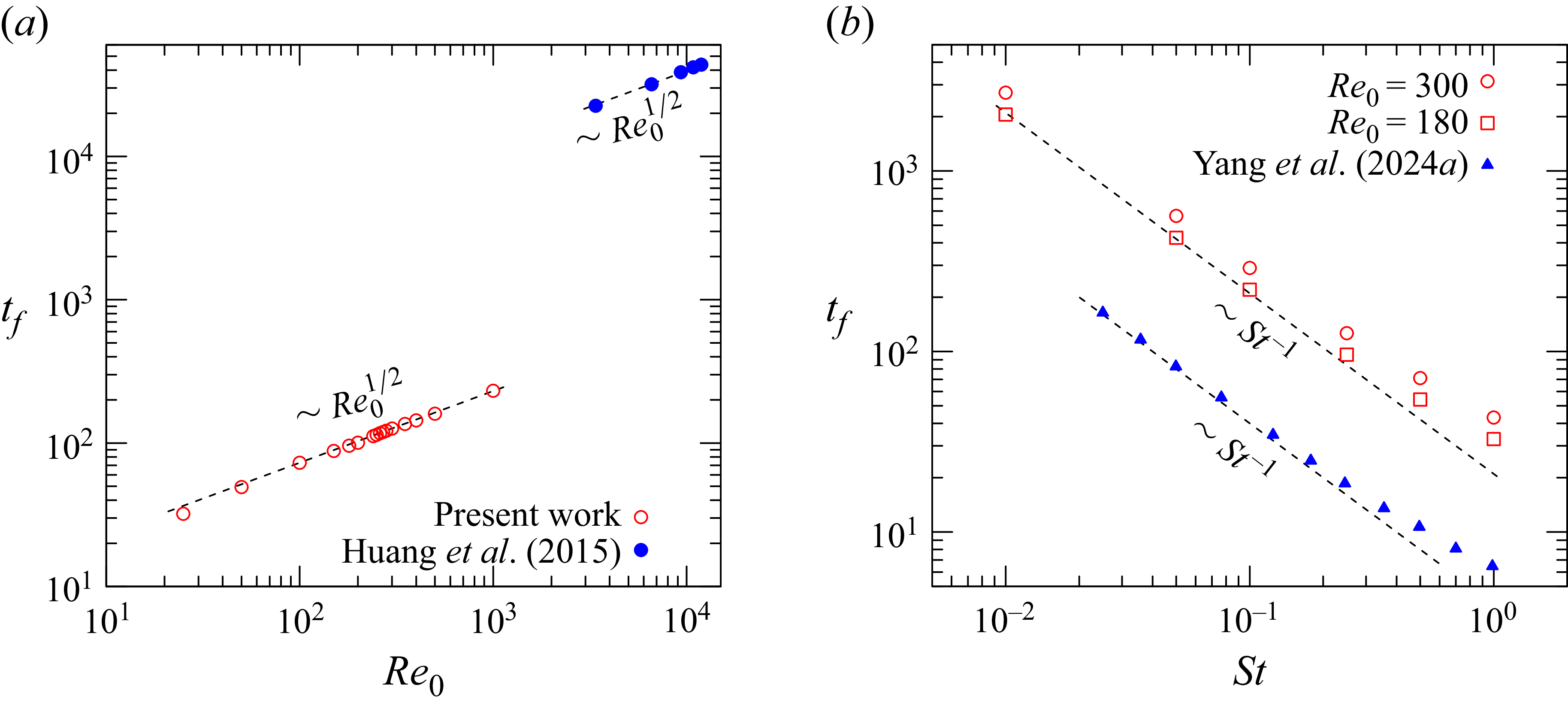


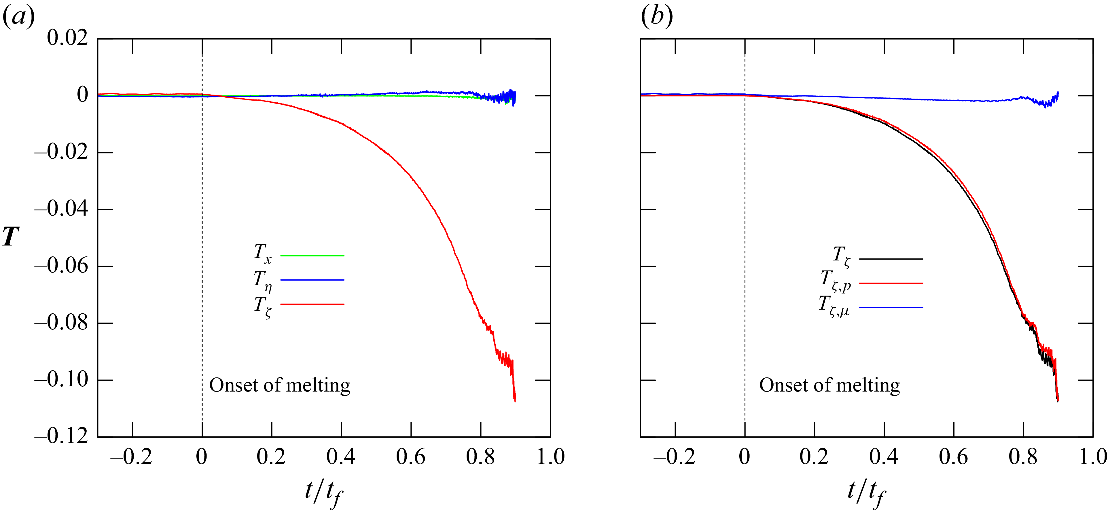


 Open access

