


I. Introduction
The COVID-19 pandemic once again underscored the central role of monetary policy in stabilizing the economy, supporting consumption, investment, and production, while calming financial and credit markets. Beyond its stabilizing function, monetary policy is also a key driver of asset prices and risk premia (see, e.g., Savor and Wilson (Reference Savor and Wilson2014), Lucca and Moench (Reference Lucca and Moench2015), Neuhierl and Weber (Reference Neuhierl and Weber2018), and Ozdagli and Velikov (Reference Ozdagli and Velikov2020)). Nominal price rigidity—the inability of firms to adjust output prices immediately to nominal shocks—is the leading mechanism through which monetary policy affects the real economy. Price stickiness matters not only for aggregate transmission but also for explaining cross-sectional differences in firms’ responses to shocks. Recent studies using microdata from official price statistics show that firm-level price rigidity correlates with stock returns, leverage choices, and the transmission of fiscal and monetary policy.Footnote 1 However, little is known about how output price stickiness shapes firms’ credit risk, cash holdings, or debt structure.
We develop a capital structure model to examine how price stickiness shapes firms’ financing choices and credit risk. Firms produce differentiated goods using a risky technology, financed through short- and long-term debt, equity, and cash. They optimally choose leverage and debt maturity by balancing the tax benefits of debt against bankruptcy costs. To avoid default, firms may issue seasoned equity, subject to flotation costs, and hold cash to buffer adverse shocks, despite agency costs. Crucially, firms differ in their ability to adjust output prices. This heterogeneity in price rigidity affects operating flexibility and thereby default risk. Our model yields several testable predictions. Firms with more flexible output prices tend to have higher leverage and a greater reliance on long-term debt, while holding less precautionary cash, facing lower borrowing costs, and being subject to less stringent debt covenants. In addition, the cost of debt for sticky-price firms is more sensitive to monetary policy shocks (MPSs) and rises more sharply in response to exogenous increases in cash flow volatility, both through default risk and risk premium channels.
To test these predictions, we use micro-level data from the Bureau of Labor Statistics’ (BLS) Producer Price Index (PPI) to construct measures of nominal price rigidity. We merge these with financial data from CRSP and Compustat, cost of debt information from Mergent FISD and TRACE, and loan covenant data from Thomson Reuters LPC DealScan. We first show that firms with the stickiest prices hold significantly more precautionary cash. Inflexible-price firms, on average, maintain cash buffers about 22% larger than their flexible-price counterparts. This result remains robust after controlling for standard determinants of cash holdings, unobserved macroeconomic and financial risk factors, and industry-specific characteristics. Next, we test how debt characteristics vary with nominal output price rigidity. Sticky-price firms face higher issuance credit spreads, making debt more costly, and their bonds trade at lower prices in secondary markets. On average, these firms also have shorter debt maturity and tighter loan covenants.
After documenting unconditional differences, we examine how firms respond to shocks. We show that nominal rigidities shape the transmission of monetary policy to asset prices and firm behavior. Using the MPS measure of Gorodnichenko and Weber (Reference Gorodnichenko and Weber2016), we analyze how squared credit spreads of flexible- and inflexible-price firms respond to monetary surprises. A hypothetical 25- basis-point (bps) shock increases conditional credit spread volatility by about 9 bps more for fully sticky-price firms than for fully flexible-price firms. Second, our framework predicts that credit spreads respond more strongly to uncertainty shocks (e.g., volatility of cash flows or profitability) for firms with greater nominal price rigidity. To test this prediction, we use the 2008 Lehman Brothers bankruptcy, an unexpected and severe uncertainty shock, as in Chodorow-Reich (Reference Chodorow-Reich2014) and Ivashina and Scharfstein (Reference Ivashina and Scharfstein2010). As the largest bankruptcy in U.S. history, it surprised market participants and triggered the Dow Jones’ biggest point drop since the Sept. 11, 2001 attacks. Consistent with the model’s predictions, credit spreads of inflexible-price firms rose significantly more than those of flexible-price firms following the Lehman Brothers collapse. Using bond-level data, the immediate differential increase, from 2 months before to 2 months after the shock, ranges from 172 to 243 bps.
Third, we refine our analysis by exploiting cross-sectional variation in firms’ financial constraints. The model predicts that sticky-price firms with higher refinancing costs should see a larger increase in credit spreads in response to uncertainty shocks. We test this prediction using exposure to rollover risk (He and Xiong (Reference He and Xiong2012)) around the Lehman Brothers bankruptcy in a triple-difference specification. All else equal, firms with refinancing needs when credit spreads spiked after the bankruptcy likely faced higher refinancing costs. Prior studies, including Almeida, Campello, Laranjeira, and Weisbenner (Reference Almeida, Campello, Laranjeira and Weisbenner2011) and Nagler (Reference Nagler2020), show that rollover risk is a predetermined channel amplifying credit risk. We measure rollover risk as the share of debt maturing in 2009. Consistent with the model, inflexible-price firms with high rollover risk experienced significantly larger increases in credit spreads following the Lehman collapse.
Taken together, the evidence supports our model’s predictions and shows that output price rigidity is a key determinant of firms’ financial policies and credit risk, as well as a central channel through which monetary policy affects asset prices.
We contribute to the literature on nominal rigidities and financial outcomes. Using PPI micro data in high-frequency event studies around Federal Open Market Committee (FOMC) announcements, Gorodnichenko and Weber (Reference Gorodnichenko and Weber2016) provide evidence consistent with a New Keynesian view of price stickiness. Weber (Reference Weber2015) shows that sticky-price firms earn a 4% return premium annually in the cross section of stock returns, while D’Acunto et al. (Reference D’Acunto, Liu, Pflueger and Weber2018) link price stickiness to persistent differences in financial leverage across firms. Our key contribution is to show that output price stickiness influences firms’ credit risk, cash holdings, and debt structure, spanning maturity, pricing, and covenants. We document a persistent wedge in issuance and secondary market credit spreads between flexible- and sticky-price firms. Sticky-price firms also exhibit greater sensitivity to uncertainty shocks. This heightened sensitivity drives higher precautionary cash holdings, prompting creditors to demand tighter covenants and shorter debt maturity.
While New Keynesian models emphasize price stickiness in transmitting nominal shocks, wage rigidities can similarly affect firms through labor costs. Recent work shows that cross-industry variation in wage rigidity and labor shares drives return predictability, credit risk, and helps explain asset pricing puzzles (Belo, Lin, and Bazdresch (Reference Belo, Lin and Bazdresch2014), Favilukis and Lin (Reference Favilukis and Lin2016a), (2016Reference Favilukis and Linb), Favilukis, Lin, and Zhao (Reference Favilukis, Lin and Zhao2020), and Belo, Donangelo, Lin, and Luo (Reference Belo, Donangelo, Lin and Luo2023)). Like these studies, we examine rigidities in financial markets, but focus on nominal frictions on the revenue side rather than real frictions on the cost side. Robustness tests confirm that wage and price stickiness are both important and complementary drivers of credit risk.Footnote 2
Our article also relates to studies on the role of sticky leverage in shaping credit risk. Bhamra, Fisher, and Kuehn (Reference Bhamra, Fisher and Kuehn2011), Kang and Pflueger (Reference Kang and Pflueger2015), and Gomes, Jermann, and Schmid (Reference Gomes, Jermann and Schmid2016) model how nominal debt contracts affect credit risk following unexpected price level changes. Corhay and Tong (Reference Corhay and Tong2026) show that sticky leverage can disrupt aggregate credit supply when financial intermediaries are constrained, while Bhamra, Dorion, Jeanneret, and Weber (Reference Bhamra, Dorion, Jeanneret and Weber2018) examine how sticky leverage and cash flows jointly influence credit risk and equity valuations.Footnote 3 Table 1 highlights our contribution. In contrast to these studies, we focus on how sticky output prices affect credit risk and provide new evidence on the pricing and structure of debt across firms. In related work, Gu, Hackbarth, and Johnson (Reference Gu, Hackbarth and Johnson2018) and Gu, Hackbarth, and Li (Reference Gu, Hackbarth and Li2019) examine how scale irreversibility influences firm risk and leverage. Like them, we show that firm-level frictions shape exposure to aggregate risk and influence risk pricing in financial markets.

Our focus on nominal price rigidities and credit risk also contributes to the extensive literature on credit spread determinants (e.g., Merton (Reference Merton1974), Collin-Dufresne, Goldstein, and Martin (Reference Collin-Dufresne, Goldstein and Martin2001), Campbell and Taksler (Reference Campbell and Taksler2003), Blanco, Brennan, and Marsh (Reference Blanco, Brennan and Marsh2005), Chen, Lesmond, and Wei (Reference Chen, Lesmond and Wei2007), Bharath and Shumway (Reference Bharath and Shumway2008), Zhang, Zhou, and Zhu (Reference Zhang, Zhou and Zhu2009), Bongaerts, De Jong, and Driessen (Reference Bongaerts, De Jong and Driessen2011), Acharya, Amihud, and Bharath (Reference Acharya, Amihud and Bharath2013b), Corhay (Reference Corhay2017), Siriwardane (Reference Siriwardane2019), Augustin and Izhakian (Reference Augustin and Izhakian2020), and Chen, Dou, Guo, and Ji (Reference Chen, Dou, Guo and Ji2026)). We show that firms’ inability to adjust output prices creates a persistent wedge in the cost of debt between sticky- and flexible-price firms. We also find that sticky-price firms hold more cash, reflecting their heightened sensitivity to cash flow shocks. This result connects to research on precautionary savings driven by elevated credit risk (e.g., Bolton, Chen, and Wang (Reference Bolton, Chen and Wang2014)), as well as studies showing that firms facing stricter creditors (Subrahmanyam, Tang, and Wang (Reference Subrahmanyam, Tang and Wang2017)) or greater refinancing risk (Harford, Klasa, and Maxwell (Reference Harford, Klasa and Maxwell2014)) tend to hold more cash. Our findings also align with evidence that firms prefer cash to credit lines for liquidity management (Acharya, Davydenko, and Strebulaev (Reference Acharya, Davydenko and Strebulaev2012), Acharya, Almeida, and Campello (Reference Acharya, Almeida and Campello2013a)). Lin, Schmid, and Weisbach (Reference Lin, Schmid and Weisbach2021) show that greater production price risk is associated with higher cash holdings in the electricity sector. We complement their work by grounding our analysis in a theoretical framework and focusing on output-price flexibility rather than production technology. Unlike their industry-specific study, we measure price adjustment frequency across a broad set of firms and industries. In addition to cash holdings, we also examine how price stickiness relates to debt maturity, borrowing costs, and covenant tightness.
Finally, we build on a large macroeconomic literature examining the determinants and implications of output price stickiness. Zbaracki, Ritson, Levy, Dutta, and Bergen (Reference Zbaracki, Ritson, Levy, Dutta and Bergen2004) estimate that nominal price adjustments cost a major U.S. manufacturer 1.22% of total revenue and 20.03% of net profit. Using Consumer Price Index (CPI) microdata, Bils and Klenow (Reference Bils and Klenow2004) and Nakamura and Steinsson (Reference Nakamura and Steinsson2008) show that prices are typically fixed for about 6 months, with substantial cross-industry variation, findings confirmed for producer prices by Goldberg and Hellerstein (Reference Goldberg and Hellerstein2011). Other contributions include Eichenbaum, Jaimovich, and Rebelo (Reference Eichenbaum, Jaimovich and Rebelo2011), Anderson, Jaimovich, and Simester (Reference Anderson, Jaimovich and Simester2015), and Kehoe and Midrigan (Reference Kehoe and Midrigan2015). More recent work by Pasten et al. (Reference Pasten, Schoenle and Weber2020), (Reference Pasten, Schoenle and Weber2024) and Cox, Müller, Pasten, Schoenle, and Weber (Reference Cox, Müller, Pasten, Schoenle and Weber2024) explores how heterogeneity in price stickiness affects the transmission of idiosyncratic, monetary, and fiscal shocks. See Klenow and Malin (Reference Klenow, Malin, Friedman and Woodford2010) for a review of the recent literature on price rigidity using micro price data.
II. Model
This section presents a partial equilibrium model that illustrates how price stickiness shapes firms’ financing decisions and credit risk. Greater price rigidity reduces operational flexibility, making sticky-price firms more exposed to adverse shocks and thus riskier. In equilibrium, price stickiness results in lower leverage, higher precautionary cash holdings, a greater default probability, wider credit spreads, and shorter debt maturity. Because debt covenants help mitigate shareholder–creditor agency conflicts, firms with inflexible output prices face tighter covenants than those with flexible prices.
A. Economic Environment
The economy consists of a continuum of firms operating a linear production technology over three periods. Firms differ in their ability to adjust nominal output prices, governed by their degree of price stickiness. A representative investor holds all claims with preferences captured by an exogenous pricing kernel. Figure 1 outlines the sequence of events.
Figure 1 illustrates the timeline of the firm’s decision-making process. At $ t=0 $
, firms choose their optimal capital structure, including equity, debt, and precautionary cash holdings. At
$ t=0 $
, firms choose their optimal capital structure, including equity, debt, and precautionary cash holdings. At $ t=1 $
, the first IID profit shock is realized. Firms revise output prices with probability
$ t=1 $
, the first IID profit shock is realized. Firms revise output prices with probability $ 1-\theta $
, determine production capacity, and decide whether to adjust cash holdings, raise external equity, or default. If no default occurs, short-term debt is repaid, and residual cash flows are paid as dividends. At
$ 1-\theta $
, determine production capacity, and decide whether to adjust cash holdings, raise external equity, or default. If no default occurs, short-term debt is repaid, and residual cash flows are paid as dividends. At $ t=2 $
, a second IID profit shock is realized. As in
$ t=2 $
, a second IID profit shock is realized. As in $ t=1 $
, firms may revise prices with probability
$ t=1 $
, firms may revise prices with probability $ \left(1-\theta \right) $
, set production, adjust cash, issue equity, or default. If solvent, they repay long-term debt and distribute remaining cash flows as dividends.
$ \left(1-\theta \right) $
, set production, adjust cash, issue equity, or default. If solvent, they repay long-term debt and distribute remaining cash flows as dividends.

At $ t=0 $
, firms raise financing through equity, one-period and two-period debt, and choose precautionary cash holdings to buffer against future shocks. At
$ t=0 $
, firms raise financing through equity, one-period and two-period debt, and choose precautionary cash holdings to buffer against future shocks. At $ t=1 $
, each firm observes its idiosyncratic productivity shock along with all aggregate shocks, then chooses its production level and nominal price. Price setting is inflexible, as firms face a positive probability of being unable to adjust prices in response to shocks. The firm repays its one-period debt, may update its cash holdings, and, if short on cash, can issue new equity or default. Any residual free cash flow is paid out as dividends to shareholders. At
$ t=1 $
, each firm observes its idiosyncratic productivity shock along with all aggregate shocks, then chooses its production level and nominal price. Price setting is inflexible, as firms face a positive probability of being unable to adjust prices in response to shocks. The firm repays its one-period debt, may update its cash holdings, and, if short on cash, can issue new equity or default. Any residual free cash flow is paid out as dividends to shareholders. At $ t=2 $
, surviving firms experience a second idiosyncratic productivity shock together with aggregate shocks. They choose output prices (subject to price rigidity), realize profits, and decide whether to default. If solvent, the firm repays its long-term debt and distributes remaining cash flows to shareholders as dividends. The firm then exits the market.
$ t=2 $
, surviving firms experience a second idiosyncratic productivity shock together with aggregate shocks. They choose output prices (subject to price rigidity), realize profits, and decide whether to default. If solvent, the firm repays its long-term debt and distributes remaining cash flows to shareholders as dividends. The firm then exits the market.
1. Production
Each firm $ i $
operates a linear production technology that produces output
$ i $
operates a linear production technology that produces output $ {y}_{it}^s $
using a predetermined capital stock
$ {y}_{it}^s $
using a predetermined capital stock $ {k}_{i0} $
and a variable input
$ {k}_{i0} $
and a variable input $ {l}_{it} $
(e.g., labor), purchased in a competitive market at a real unit cost
$ {l}_{it} $
(e.g., labor), purchased in a competitive market at a real unit cost $ W $
:
$ W $
:
 $$ {y}_{it}^s={\tilde{X}}_{it}{k}_{i0}{l}_{it}. $$
Here, $ {\tilde{X}}_{it} $
denotes a firm-specific IID log-normal productivity shock, with
$ {\tilde{X}}_{it} $
denotes a firm-specific IID log-normal productivity shock, with $ \log \left({\tilde{X}}_{it}\right)\sim \mathcal{N}\left({\mu}_t,{\sigma}_t^2\right) $
. While realizations of
$ \log \left({\tilde{X}}_{it}\right)\sim \mathcal{N}\left({\mu}_t,{\sigma}_t^2\right) $
. While realizations of $ {\tilde{X}}_{it} $
are unknown ex ante, their distribution is common knowledge and identical across firms. The conditional moments
$ {\tilde{X}}_{it} $
are unknown ex ante, their distribution is common knowledge and identical across firms. The conditional moments $ {\mu}_t $
and
$ {\mu}_t $
and $ {\sigma}_t $
may vary over time to capture aggregate productivity or uncertainty shocks (e.g., Bloom (Reference Bloom2009)). Let
$ {\sigma}_t $
may vary over time to capture aggregate productivity or uncertainty shocks (e.g., Bloom (Reference Bloom2009)). Let $ \Phi \left(\cdot \right) $
and
$ \Phi \left(\cdot \right) $
and $ \phi \left(\cdot \right) $
denote the cumulative distribution and probability density functions of the standard normal distribution, respectively.
$ \phi \left(\cdot \right) $
denote the cumulative distribution and probability density functions of the standard normal distribution, respectively.
The real demand for firm $ i $
’s product,
$ i $
’s product, $ {y}_{it}^d $
, depends on the nominal price
$ {y}_{it}^d $
, depends on the nominal price $ {p}_{it} $
it charges relative to the aggregate price level
$ {p}_{it} $
it charges relative to the aggregate price level $ {P}_t $
:
$ {P}_t $
:
 $$ {y}_{it}^d={\left(\frac{p_{it}}{P_t}\right)}^{-\nu }, $$
where $ \nu >1 $
denotes the elasticity of demand; higher values of
$ \nu >1 $
denotes the elasticity of demand; higher values of $ \nu $
imply more elastic demand and thus less market power for the firm.
$ \nu $
imply more elastic demand and thus less market power for the firm.
Imposing the equilibrium condition $ {y}_{it}^d={y}_{it}^s={y}_{it} $
, the firm’s real profit (normalized by
$ {y}_{it}^d={y}_{it}^s={y}_{it} $
, the firm’s real profit (normalized by $ {P}_t $
) is defined as revenue net of operating costs:
$ {P}_t $
) is defined as revenue net of operating costs:
 $$ {h}_{it}=\left(\frac{p_{it}}{P_t}\right){y}_{it}-{Wl}_{it}-{fk}_{i0}\times {\unicode{x1D7D9}}_{t=1}, $$
where $ {p}_{it} $
is firm
$ {p}_{it} $
is firm $ i $
’s nominal output price and
$ i $
’s nominal output price and $ {P}_t $
is the aggregate price level. The term
$ {P}_t $
is the aggregate price level. The term $ f $
denotes a fixed cost of maintaining the capital stock for the next period, incurred only in periods 0 and 1, since the firm operates for three periods. Without loss of generality, we normalize the initial capital stock
$ f $
denotes a fixed cost of maintaining the capital stock for the next period, incurred only in periods 0 and 1, since the firm operates for three periods. Without loss of generality, we normalize the initial capital stock $ {k}_{i0} $
to one.
$ {k}_{i0} $
to one.
2. Price Stickiness
Following Calvo (Reference Calvo1983), we assume that at the start of each period, after all relevant shocks are realized, each firm faces an idiosyncratic shock $ {\zeta}_{it}\in \left\{0,1\right\} $
that determines its ability to adjust output prices. If
$ {\zeta}_{it}\in \left\{0,1\right\} $
that determines its ability to adjust output prices. If $ {\zeta}_{it}=1 $
, the firm can freely reoptimize and set a new price. If
$ {\zeta}_{it}=1 $
, the firm can freely reoptimize and set a new price. If $ {\zeta}_{it}=0 $
, the firm must continue selling at the previous period’s price
$ {\zeta}_{it}=0 $
, the firm must continue selling at the previous period’s price $ {p}_{it-1} $
. The conditional probability of not adjusting prices is denoted by
$ {p}_{it-1} $
. The conditional probability of not adjusting prices is denoted by $ \theta \in \left[0,1\right] $
, which captures the degree of price rigidity. The limiting case
$ \theta \in \left[0,1\right] $
, which captures the degree of price rigidity. The limiting case $ \theta =0 $
corresponds to fully flexible prices.
$ \theta =0 $
corresponds to fully flexible prices.
3. Financing
Debt: At $ t=0 $
, the firm chooses its issuance of short- and long-term real debt. Short-term debt matures at
$ t=0 $
, the firm chooses its issuance of short- and long-term real debt. Short-term debt matures at $ t=1 $
, whereas long-term debt matures at
$ t=1 $
, whereas long-term debt matures at $ t=2 $
. Following Leland (Reference Leland1994), (Reference Leland1998), the firm commits to this initial debt schedule but may issue new equity in future periods. Equity holders retain the option to default when the equity value turns negative, with zero recovery for creditors.Footnote
4 These deadweight default costs raise the effective cost of debt financing relative to equity.
$ t=2 $
. Following Leland (Reference Leland1994), (Reference Leland1998), the firm commits to this initial debt schedule but may issue new equity in future periods. Equity holders retain the option to default when the equity value turns negative, with zero recovery for creditors.Footnote
4 These deadweight default costs raise the effective cost of debt financing relative to equity.
To ensure an interior solution for the optimal debt-equity mix at $ t=0 $
, we assume that debt provides benefits to shareholders. For instance, interest payments are tax-deductible, offering an advantage over equity. However, tax benefits alone cannot fully explain observed leverage levels (e.g., Graham (Reference Graham2000)). More broadly, debt may also help mitigate agency and informational frictions, as argued by Myers and Majluf (Reference Myers and Majluf1984) and Jensen (Reference Jensen1986).
$ t=0 $
, we assume that debt provides benefits to shareholders. For instance, interest payments are tax-deductible, offering an advantage over equity. However, tax benefits alone cannot fully explain observed leverage levels (e.g., Graham (Reference Graham2000)). More broadly, debt may also help mitigate agency and informational frictions, as argued by Myers and Majluf (Reference Myers and Majluf1984) and Jensen (Reference Jensen1986).
Following Gourio (Reference Gourio2013) and Kang and Pflueger (Reference Kang and Pflueger2015), we capture the present value of debt benefits in reduced form by assuming that the firm receives $ \left(1+{\chi}^S\right)>1 $
and
$ \left(1+{\chi}^S\right)>1 $
and $ \left(1+{\chi}^L\right)>1 $
for each dollar of short- and long-term debt issued, respectively. Higher values of
$ \left(1+{\chi}^L\right)>1 $
for each dollar of short- and long-term debt issued, respectively. Higher values of $ {\chi}^S $
and
$ {\chi}^S $
and $ {\chi}^L $
increase the appeal of debt, raising leverage. Their difference determines the relative attractiveness of short- versus long-term debt and thus shapes the firm’s optimal maturity structure. In our numerical analysis, we calibrate these parameters jointly to match observed firm-level leverage and the ratio of long- to short-term debt.
$ {\chi}^L $
increase the appeal of debt, raising leverage. Their difference determines the relative attractiveness of short- versus long-term debt and thus shapes the firm’s optimal maturity structure. In our numerical analysis, we calibrate these parameters jointly to match observed firm-level leverage and the ratio of long- to short-term debt.
The total proceeds from debt issuance at time $ t=0 $
are given by:
$ t=0 $
are given by:
 $$ \left(1+{\chi}^S\right)\;{q}_{i0}^S{b}_i^S+\left(1+{\chi}^L\right)\;{q}_{i0}^L{b}_i^L, $$
where $ {b}_i^S $
(
$ {b}_i^S $
( $ {b}_i^L $
) is the amount of short-term (long-term) real debt issued, and
$ {b}_i^L $
) is the amount of short-term (long-term) real debt issued, and $ {q}_{i0}^S $
(
$ {q}_{i0}^S $
( $ {q}_{i0}^L $
) denotes its market price at
$ {q}_{i0}^L $
) denotes its market price at $ t=0 $
.Footnote
5
$ t=0 $
.Footnote
5
Debt is issued in a competitive, rational lending market. Let $ {\unicode{x1D7D9}}_{it}^{\mathrm{survival}} $
denote a survival indicator equal to 1 if firm
$ {\unicode{x1D7D9}}_{it}^{\mathrm{survival}} $
denote a survival indicator equal to 1 if firm $ i $
does not default in period
$ i $
does not default in period $ t $
, and 0 otherwise. The market value of debt equals the expected present value of future cash flows:
$ t $
, and 0 otherwise. The market value of debt equals the expected present value of future cash flows:
 $$ {q}_{it}^S={\unicode{x1D53C}}_t\left[{M}_{t+1}\times {\unicode{x1D7D9}}_{it+1}^{\mathrm{survival}}\right],\hskip1em \mathrm{for}\;t=0,1, $$
 $$ {q}_{i0}^L={\unicode{x1D53C}}_0\left[{M}_1\times {q}_{i1}^S\right], $$
where $ {M}_t $
denotes the real stochastic discount factor. The firm’s default decision is endogenous and determined by equity holders’ optimization problem, discussed in Section II.C.
$ {M}_t $
denotes the real stochastic discount factor. The firm’s default decision is endogenous and determined by equity holders’ optimization problem, discussed in Section II.C.
Equity: At time $ t=0 $
, the firm can issue equity without cost. In subsequent periods, it may raise external equity at a cost
$ t=0 $
, the firm can issue equity without cost. In subsequent periods, it may raise external equity at a cost $ \lambda $
per dollar issued (e.g., Jermann and Quadrini (Reference Jermann and Quadrini2012), Eisfeldt and Muir (Reference Eisfeldt and Muir2016)), capturing flotation costs or agency frictions (Hennessy and Whited (Reference Hennessy and Whited2007)). As shown in Section II.E, costly external financing creates a wedge between the shadow value of internal and external funds, inducing effective risk aversion and making precautionary cash holdings a key tool for mitigating financing frictions. Unlike debt holders, equity holders are entitled to residual cash flows and benefit from limited liability, allowing them to walk away with zero payout in the event of default.
$ \lambda $
per dollar issued (e.g., Jermann and Quadrini (Reference Jermann and Quadrini2012), Eisfeldt and Muir (Reference Eisfeldt and Muir2016)), capturing flotation costs or agency frictions (Hennessy and Whited (Reference Hennessy and Whited2007)). As shown in Section II.E, costly external financing creates a wedge between the shadow value of internal and external funds, inducing effective risk aversion and making precautionary cash holdings a key tool for mitigating financing frictions. Unlike debt holders, equity holders are entitled to residual cash flows and benefit from limited liability, allowing them to walk away with zero payout in the event of default.
Cash: Each period, firms decide whether to hold cash as a precaution against future productivity shocks. Holding cash can reduce future financing costs. To prevent firms from relying excessively on cash and thereby neutralizing financing frictions, we introduce an agency problem following Nikolov and Whited (Reference Nikolov and Whited2014), in which managers may divert free cash flows for private benefit. We model these agency costs in reduced form, similar to our treatment of debt benefits. Let $ {x}_{it} $
denote the firm’s real cash balance at the end of period
$ {x}_{it} $
denote the firm’s real cash balance at the end of period $ t $
. We assume the firm incurs a cost of
$ t $
. We assume the firm incurs a cost of $ \frac{\psi {x}_{it}}{2} $
per dollar of cash held, where
$ \frac{\psi {x}_{it}}{2} $
per dollar of cash held, where $ \psi >0 $
. The net cash flow associated with cash balances is then given by:
$ \psi >0 $
. The net cash flow associated with cash balances is then given by:
 $$ {x}_{it-1}-{x}_{it}\left(1+\frac{\psi }{2}{x}_{it}\right). $$
This specification implies a quadratic cost of holding cash, governed by the parameter $ \psi $
. In our numerical analysis, we calibrate
$ \psi $
. In our numerical analysis, we calibrate $ \psi $
to match the average cash holdings observed in the data.
$ \psi $
to match the average cash holdings observed in the data.
B. Objective Function
The firm’s objective is to maximize equity value by making a sequence of financing and production decisions, subject to product demand and fair debt pricing. For simplicity, we omit the $ i $
-subscript unless needed for clarity.
$ i $
-subscript unless needed for clarity.
In period $ t=0 $
, the entrepreneur is unlevered and does not produce. The problem reduces to choosing short- and long-term debt levels,
$ t=0 $
, the entrepreneur is unlevered and does not produce. The problem reduces to choosing short- and long-term debt levels, $ {b}^S $
and
$ {b}^S $
and $ {b}^L $
, and initial cash holdings
$ {b}^L $
, and initial cash holdings $ {x}_0 $
, to maximize total proceeds from debt and equity issuanceFootnote
6:
$ {x}_0 $
, to maximize total proceeds from debt and equity issuanceFootnote
6:
 $$ {\displaystyle \begin{array}{l}\underset{b^S,{b}^L,{x}_0}{\max}\left\{{\unicode{x1D53C}}_0\left[{M}_1{V}_1\left({\tilde{\zeta}}_1,{\tilde{X}}_1,{z}_1,{\Upsilon}_1\right)\right]-{x}_0-\frac{\psi }{2}{\left({x}_0\right)}^2\right.\\ {}\left.\hskip2em +\left(1+{\chi}^S\right){q}_0^S\Big({\tilde{\zeta}}_1,{\tilde{X}}_1,{z}_1,{\Upsilon}_1\left)\times {b}^S+\left(1+{\chi}^L\right){q}_0^L\right({\tilde{\zeta}}_1,{\tilde{X}}_1,{z}_1,{\Upsilon}_1\Big)\times {b}^L-f\right\},\end{array}} $$
subject to the breakeven conditions (5) and (6), which determine the equilibrium prices of short- and long-term debt, respectively.
The value of equity $ {V}_1 $
and the debt prices
$ {V}_1 $
and the debt prices $ {q}_0^S $
and
$ {q}_0^S $
and $ {q}_0^L $
depend on a set of state variables summarized by the vector
$ {q}_0^L $
depend on a set of state variables summarized by the vector $ \left({\tilde{\zeta}}_t,{\tilde{X}}_t,{z}_t,{\Upsilon}_t\right) $
. Here,
$ \left({\tilde{\zeta}}_t,{\tilde{X}}_t,{z}_t,{\Upsilon}_t\right) $
. Here, $ {z}_t\equiv \left({b}^S,{b}^L,{x}_{t-1},{p}_{t-1}\right) $
captures firm-specific states, while
$ {z}_t\equiv \left({b}^S,{b}^L,{x}_{t-1},{p}_{t-1}\right) $
captures firm-specific states, while $ {\Upsilon}_t $
denotes aggregate state variables. Accordingly, the firm internalizes how its financing decisions affect the market values of both equity and debt.
$ {\Upsilon}_t $
denotes aggregate state variables. Accordingly, the firm internalizes how its financing decisions affect the market values of both equity and debt.
In periods $ t>0 $
, the firm chooses its production quantity, output price, and cash holdings
$ t>0 $
, the firm chooses its production quantity, output price, and cash holdings $ {x}_t $
to maximize equity value. If the dividend is negative, the firm may issue seasoned equity, incurring a flotation cost
$ {x}_t $
to maximize equity value. If the dividend is negative, the firm may issue seasoned equity, incurring a flotation cost $ \lambda $
. Alternatively, it declares bankruptcy when the firm value is negative. The firm faces two types of idiosyncratic uncertainty: A productivity shock
$ \lambda $
. Alternatively, it declares bankruptcy when the firm value is negative. The firm faces two types of idiosyncratic uncertainty: A productivity shock $ {\tilde{X}}_t\in \left[0,+\infty \right) $
and a pricing shock
$ {\tilde{X}}_t\in \left[0,+\infty \right) $
and a pricing shock $ {\zeta}_t\in \left\{0,1\right\} $
, along with a sequence of aggregate shocks. The real market value of equity satisfies the following recursive formulation for
$ {\zeta}_t\in \left\{0,1\right\} $
, along with a sequence of aggregate shocks. The real market value of equity satisfies the following recursive formulation for $ t=1,2 $
:
$ t=1,2 $
:
 $$ {\displaystyle \begin{array}{l}{V}_t\left({\Xi}_t\right)=\underset{x_t,{p}_t\left({\tilde{\zeta}}_t=1\right),{l}_t}{\max}\left\{\max \left({d}_t\left({\Xi}_t\right)+{\mathrm{E}}_t\left[{M}_{t+1}{V}_{t+1}\left({\Xi}_{t+1}\right)\right],0\right)\right\},\\ {}\hskip5.7em \mathrm{subject}\ \mathrm{to}:\hskip1em {y}_t\left({\tilde{\zeta}}_t\right)={\left(\frac{p_t\left({\tilde{\zeta}}_t\right)}{P_t}\right)}^{-\nu}\end{array}} $$
where $ {p}_t\left({\tilde{\zeta}}_t\right)={\unicode{x1D7D9}}_{\left\{{\tilde{\zeta}}_t=0\right\}}\times {p}_{t-1}+{\unicode{x1D7D9}}_{\left\{{\tilde{\zeta}}_t=1\right\}}\times {p}_t $
captures the fact that the firm can only optimize its nominal output price when
$ {p}_t\left({\tilde{\zeta}}_t\right)={\unicode{x1D7D9}}_{\left\{{\tilde{\zeta}}_t=0\right\}}\times {p}_{t-1}+{\unicode{x1D7D9}}_{\left\{{\tilde{\zeta}}_t=1\right\}}\times {p}_t $
captures the fact that the firm can only optimize its nominal output price when $ {\tilde{\zeta}}_t=1 $
and
$ {\tilde{\zeta}}_t=1 $
and $ {\Xi}_t\equiv \left({\tilde{\zeta}}_t,{\tilde{X}}_t,{z}_t,{\Upsilon}_t\right) $
summarizes the set of state variables. The real dividends (i.e., normalized by
$ {\Xi}_t\equiv \left({\tilde{\zeta}}_t,{\tilde{X}}_t,{z}_t,{\Upsilon}_t\right) $
summarizes the set of state variables. The real dividends (i.e., normalized by $ {P}_t $
) paid by the firm at
$ {P}_t $
) paid by the firm at $ t=1,2 $
are:
$ t=1,2 $
are:
 $$ {d}_1\left({\Xi}_1\right)=\frac{h_1\left({\tilde{\zeta}}_1,{\tilde{X}}_1,{z}_1,{\Upsilon}_1\right)+{x}_0-{x}_1\left(1+\psi \right)-{b}^S-f}{1-\lambda \times {\unicode{x1D7D9}}_{\left\{{d}_1<0\right\}}}, $$
 $$ {d}_2\left({\Xi}_2\right)=\frac{h_2\left({\tilde{\zeta}}_2,{\tilde{X}}_2,{z}_2,{\Upsilon}_2\right)+{x}_1-{x}_2\left(1+\psi \right)-{b}^L}{1-\lambda \times {\unicode{x1D7D9}}_{\left\{{d}_2<0\right\}}}. $$
C. Optimal Policies
We now describe the firm’s optimal policies. Since the firm’s labor decision is static, the model can be solved in two steps.
First, we solve the firm’s cost-minimization problem: Given a target output level, the firm chooses labor to minimize production costs, yielding the marginal cost $ {\tilde{c}}_t $
as a function of firm-level productivity:
$ {\tilde{c}}_t $
as a function of firm-level productivity:
 $$ {\tilde{c}}_t=\frac{W}{{\tilde{X}}_t}. $$
The log marginal cost inherits the log-normal distribution of $ {\tilde{X}}_t $
; specifically,
$ {\tilde{X}}_t $
; specifically, $ \log \left({\tilde{c}}_t\right)\sim \mathcal{N}\left(\log (W)-{\mu}_t,{\sigma}_t^2\right) $
. For clarity, we refer to marginal cost rather than productivity throughout the remainder of the draft, noting their inverse relationship: Lower productivity implies higher marginal cost.
$ \log \left({\tilde{c}}_t\right)\sim \mathcal{N}\left(\log (W)-{\mu}_t,{\sigma}_t^2\right) $
. For clarity, we refer to marginal cost rather than productivity throughout the remainder of the draft, noting their inverse relationship: Lower productivity implies higher marginal cost.
In the second step, we solve jointly for the firm’s optimal pricing, financing, and default decisions. Given the finite horizon, this step is solved recursively. We summarize the resulting policy functions, provide economic intuition, and leave full derivations to Section A.1 of the Supplementary Material.
Pricing policy: We first solve for the optimal output price in each period, after substituting in the demand schedule. At $ t=2 $
, a flexible-price firm, knowing it will cease operations, sets its nominal price to maximize current profits. This yields a pricing policy with a constant markup of
$ t=2 $
, a flexible-price firm, knowing it will cease operations, sets its nominal price to maximize current profits. This yields a pricing policy with a constant markup of $ \nu /\left(\nu -1\right) $
over nominal marginal cost
$ \nu /\left(\nu -1\right) $
over nominal marginal cost $ {\tilde{c}}_2{P}_2 $
, that is,
$ {\tilde{c}}_2{P}_2 $
, that is,
 $$ {p}_2^{\star}\left({\tilde{c}}_2\right)=\frac{\nu }{\nu -1}{\tilde{c}}_2{P}_2. $$
In contrast, if the firm cannot adjust its output price due to price rigidity, it must continue selling at the previously set nominal price $ {p}_1 $
. This price may be suboptimal if either the marginal cost
$ {p}_1 $
. This price may be suboptimal if either the marginal cost $ {\tilde{c}}_2 $
or the aggregate price level
$ {\tilde{c}}_2 $
or the aggregate price level $ {P}_2 $
changes, exposing the firm to real and nominal risk.
$ {P}_2 $
changes, exposing the firm to real and nominal risk.
At $ t=1 $
, a flexible-price firm sets its output price to maximize the present discounted value of dividends, resulting in the following optimal pricing policy:
$ t=1 $
, a flexible-price firm sets its output price to maximize the present discounted value of dividends, resulting in the following optimal pricing policy:
 $$ \frac{p_1^{\star}\left({\tilde{c}}_1\right)}{P_1}=\left(\frac{\nu }{\nu -1}\right)\frac{{\tilde{c}}_1+\theta \left(1-\lambda \times {\unicode{x1D7D9}}_{\left\{{d}_1<0\right\}}\right){\unicode{x1D53C}}_1\left[{M}_2\left({\int}_0^{c_{\zeta_2=0}^d}{\tilde{c}}_2d\Phi \left({\tilde{c}}_2\right)\right){\left({\Pi}_2\right)}^{\nu}\right]}{1+\theta \left(1-\lambda \times {\unicode{x1D7D9}}_{\left\{{d}_1<0\right\}}\right){\unicode{x1D53C}}_1\left[{M}_2\left(\Phi \left({c}_{\zeta_2=0}^d\right){\left({\Pi}_2\right)}^{\nu -1}\right)\right]}, $$
where $ {\Pi}_2\equiv {P}_2/{P}_1 $
is the gross inflation rate between
$ {\Pi}_2\equiv {P}_2/{P}_1 $
is the gross inflation rate between $ t=1 $
and
$ t=1 $
and $ t=2 $
.
$ t=2 $
.
As in the case of $ {p}_2^{\star } $
, the optimal price at
$ {p}_2^{\star } $
, the optimal price at $ t=1 $
consists of a markup over the nominal marginal cost of production. However, because of potential price rigidity in the next period, the firm now takes into account the possibility that the price it sets today may remain fixed at
$ t=1 $
consists of a markup over the nominal marginal cost of production. However, because of potential price rigidity in the next period, the firm now takes into account the possibility that the price it sets today may remain fixed at $ t=2 $
. This exposes the firm to both real marginal cost risk, via changes in
$ t=2 $
. This exposes the firm to both real marginal cost risk, via changes in $ {\tilde{c}}_2 $
, and nominal risk, via inflation
$ {\tilde{c}}_2 $
, and nominal risk, via inflation $ {\Pi}_2 $
. The extent to which the firm incorporates these future risks into its pricing decision depends on two key forces, both ultimately shaped by the degree of price rigidity. First, a higher value of
$ {\Pi}_2 $
. The extent to which the firm incorporates these future risks into its pricing decision depends on two key forces, both ultimately shaped by the degree of price rigidity. First, a higher value of $ \theta $
increases the likelihood that the firm will be unable to adjust its price in the future, making it more forward-looking in its pricing strategy today. Second, if the firm requires external equity financing (i.e.,
$ \theta $
increases the likelihood that the firm will be unable to adjust its price in the future, making it more forward-looking in its pricing strategy today. Second, if the firm requires external equity financing (i.e., $ {d}_1<0 $
) or faces a higher probability of default, it shifts its focus toward maximizing immediate cash flows, becoming more myopic.
$ {d}_1<0 $
) or faces a higher probability of default, it shifts its focus toward maximizing immediate cash flows, becoming more myopic.
In short, price inflexibility influences the firm’s pricing behavior both directly, through the risk of being stuck with today’s price, and indirectly, by shaping its financing and default decisions. Absent price rigidity (i.e., $ \theta =0 $
) or real and nominal risk (i.e.,
$ \theta =0 $
) or real and nominal risk (i.e., $ {\tilde{c}}_1={\tilde{c}}_2 $
and
$ {\tilde{c}}_1={\tilde{c}}_2 $
and $ {\Pi}_2={\Pi}_1 $
), the firm would simply set:
$ {\Pi}_2={\Pi}_1 $
), the firm would simply set:
 $$ {p}_1^{flex}=\frac{\nu }{\nu -1}{\tilde{c}}_1{P}_1. $$
In contrast, a non-price-optimizing firm sells its output at a nominal price $ {\overline{p}}_0 $
, which we normalize to 1.
$ {\overline{p}}_0 $
, which we normalize to 1.
Default and financing policy: In each period $ t>0 $
, the firm defaults if the marginal cost shock
$ t>0 $
, the firm defaults if the marginal cost shock $ {\tilde{c}}_t $
is high enough to result in a negative equity value. The firm continues operating as long as
$ {\tilde{c}}_t $
is high enough to result in a negative equity value. The firm continues operating as long as $ {\tilde{c}}_t $
remains below the default threshold
$ {\tilde{c}}_t $
remains below the default threshold $ {c}_t^d\left({\tilde{\zeta}}_t,{z}_t,{\Upsilon}_t\right) $
. If the shock causes a liquidity shortfall, that is, a negative dividend, the firm raises funds via costly external equity issuance. These financing decisions can be summarized as follows:
$ {c}_t^d\left({\tilde{\zeta}}_t,{z}_t,{\Upsilon}_t\right) $
. If the shock causes a liquidity shortfall, that is, a negative dividend, the firm raises funds via costly external equity issuance. These financing decisions can be summarized as follows:
 $$ \left\{\begin{array}{ll}\mathrm{default}\hskip0.24em & \mathrm{if}\;{\tilde{c}}_t\ge {c}_t^d\left({\tilde{\zeta}}_t,{z}_t,{\Upsilon}_t\right)\\ {}\mathrm{issue}\;\mathrm{new}\;\mathrm{equity}\hskip0.24em & \mathrm{if}\;{c}_t^d\left({\tilde{\zeta}}_t,{z}_t,{\Upsilon}_t\right)>{\tilde{c}}_t\ge {c}_t^e\left({\tilde{\zeta}}_t,{z}_t,{\Upsilon}_t\right)\\ {}\mathrm{no}\;\mathrm{financing}\hskip0.24em & \mathrm{if}\;{\tilde{c}}_t<{c}_t^e\left({\tilde{\zeta}}_t,{z}_t,{\Upsilon}_t\right),\end{array}\right. $$
where the equity issuance threshold $ {c}_t^e\left(\cdot \right) $
and the default threshold
$ {c}_t^e\left(\cdot \right) $
and the default threshold $ {c}_t^d\left(\cdot \right) $
are implicitly defined by the following conditions (see Section 1 of the Supplementary Material for a detailed derivation):
$ {c}_t^d\left(\cdot \right) $
are implicitly defined by the following conditions (see Section 1 of the Supplementary Material for a detailed derivation):
 $$ {c}_t^e:= {d}_t\left({\tilde{\zeta}}_t,{c}_t^e,{z}_t,{\Upsilon}_t\right)=0, $$
 $$ {c}_t^d:= {V}_t\left({\tilde{\zeta}}_t,{c}_t^d,{z}_t,{\Upsilon}_t\right)=0. $$
The endogenous thresholds in equations (17) and (18) determine the default probability, $ 1-\Phi \left({c}_t^d\right) $
, and the probability of external equity issuance,
$ 1-\Phi \left({c}_t^d\right) $
, and the probability of external equity issuance, $ 1-\Phi \left({c}_t^e\right) $
. Both depend on the full set of state variables
$ 1-\Phi \left({c}_t^e\right) $
. Both depend on the full set of state variables $ \left({\tilde{\zeta}}_t,{z}_t,{\Upsilon}_t\right) $
. The degree of price inflexibility
$ \left({\tilde{\zeta}}_t,{z}_t,{\Upsilon}_t\right) $
. The degree of price inflexibility $ \theta $
plays a central role in shaping these probabilities. Firms with sticky prices cannot adjust output prices in response to real or nominal shocks, increasing their risk exposure. For instance, in the face of an adverse cost shock, they cannot raise prices to offset losses; under favorable conditions, they cannot lower prices to boost demand. As a result, sticky-price firms are endogenously riskier, all else equal.
$ \theta $
plays a central role in shaping these probabilities. Firms with sticky prices cannot adjust output prices in response to real or nominal shocks, increasing their risk exposure. For instance, in the face of an adverse cost shock, they cannot raise prices to offset losses; under favorable conditions, they cannot lower prices to boost demand. As a result, sticky-price firms are endogenously riskier, all else equal.
Figure 2 illustrates this mechanism by comparing the probability density function (pdf) of equity at $ t=2 $
for a perfectly flexible firm (solid black line) and a perfectly inflexible firm (dashed red line). The vertical line indicates the default threshold. The inflexible firm’s pdf is left-skewed and exhibits a higher default probability, demonstrating how price stickiness increases default risk and liquidity needs, thereby shaping optimal financing decisions, such as leverage and cash holdings, and ultimately affecting the equilibrium price of debt, as we show next.
$ t=2 $
for a perfectly flexible firm (solid black line) and a perfectly inflexible firm (dashed red line). The vertical line indicates the default threshold. The inflexible firm’s pdf is left-skewed and exhibits a higher default probability, demonstrating how price stickiness increases default risk and liquidity needs, thereby shaping optimal financing decisions, such as leverage and cash holdings, and ultimately affecting the equilibrium price of debt, as we show next.
Figure 2 compares the probability density function of the equity value $ {V}_2 $
at time
$ {V}_2 $
at time $ t=2 $
, for a perfectly flexible firm (solid black line) and a perfectly inflexible firm (dashed red). The vertical dotted line represents the default threshold, that is,
$ t=2 $
, for a perfectly flexible firm (solid black line) and a perfectly inflexible firm (dashed red). The vertical dotted line represents the default threshold, that is, $ {V}_2=0 $
. The calibration used to obtain these graphs is summarized in Section II.E.
$ {V}_2=0 $
. The calibration used to obtain these graphs is summarized in Section II.E.

Debt policy: We now turn to the firm’s optimal choice of long-term debt $ {b}^L $
, derived from the first-order condition with respect to
$ {b}^L $
, derived from the first-order condition with respect to $ {b}^L $
at time
$ {b}^L $
at time $ t=0 $
:
$ t=0 $
:
 $$ {\chi}^L{q}_0^L=-\left(1+{\chi}^L\right)\frac{\partial {q}_0^L}{\partial {b}^L}{b}^L-\left(1+{\chi}^S\right)\frac{\partial {q}_0^S}{\partial {b}^L}{b}^S. $$
Equation (19) shows that optimal leverage is determined through the condition that marginal benefits equal marginal costs of issuing long-term debt. The marginal benefit is the additional proceeds per dollar raised, $ {\chi}^L{q}_0^L $
. The marginal cost reflects increased default risk, which lowers the market value of both long- and short-term debt, as indicated by
$ {\chi}^L{q}_0^L $
. The marginal cost reflects increased default risk, which lowers the market value of both long- and short-term debt, as indicated by $ \partial {q}_0^H/\partial {b}^L<0 $
for
$ \partial {q}_0^H/\partial {b}^L<0 $
for $ H=L,S $
.
$ H=L,S $
.
The optimal decision for short-term debt, $ {b}^S $
, is given by:
$ {b}^S $
, is given by:
 $$ \hskip1em {\chi}^S{q}_0^S=-\left(1+{\chi}^L\right)\frac{\partial {q}_0^L}{\partial {b}^S}{b}^L-\left(1+{\chi}^S\right)\frac{\partial {q}_0^S}{\partial {b}^S}{b}^S+\underset{\mathrm{rollover}\ \mathrm{cost}}{\underbrace{\left[\frac{\lambda }{1-\lambda}\left({\mathrm{\mathbb{P}}}_1\left(\mathrm{FIN}\right)-{\mathrm{\mathbb{P}}}_1\left(\mathrm{DEF}\right)\right)\right]}}, $$
where the probabilities of raising external financing and defaulting are given by $ {\mathrm{\mathbb{P}}}_1\left(\mathrm{FIN}\right)=1-{\unicode{x1D53C}}_0\Phi \left({c}_1^e\left({\tilde{\zeta}}_1,{z}_1,{\Upsilon}_1\right)\right) $
and
$ {\mathrm{\mathbb{P}}}_1\left(\mathrm{FIN}\right)=1-{\unicode{x1D53C}}_0\Phi \left({c}_1^e\left({\tilde{\zeta}}_1,{z}_1,{\Upsilon}_1\right)\right) $
and $ {\mathrm{\mathbb{P}}}_1\left(\mathrm{DEF}\right)=1-{\unicode{x1D53C}}_0\Phi \left({c}_1^d\left({\tilde{\zeta}}_1,{z}_1,{\Upsilon}_1\right)\right) $
, respectively.
$ {\mathrm{\mathbb{P}}}_1\left(\mathrm{DEF}\right)=1-{\unicode{x1D53C}}_0\Phi \left({c}_1^d\left({\tilde{\zeta}}_1,{z}_1,{\Upsilon}_1\right)\right) $
, respectively.
As with long-term debt, the marginal benefit of issuing an additional dollar of short-term debt is the extra inflow, $ {\chi}^S{q}_0^S $
. The marginal cost consists of two components. The first two terms reflect default-related costs, mirroring the deterioration in debt prices from increased default risk. The third term—the rollover cost—captures the heightened risk of a liquidity shortfall in the next period, which may force the firm to raise costly external equity. Thus, issuing more short-term debt today increases both default risk and the likelihood of relying on external financing.
$ {\chi}^S{q}_0^S $
. The marginal cost consists of two components. The first two terms reflect default-related costs, mirroring the deterioration in debt prices from increased default risk. The third term—the rollover cost—captures the heightened risk of a liquidity shortfall in the next period, which may force the firm to raise costly external equity. Thus, issuing more short-term debt today increases both default risk and the likelihood of relying on external financing.
The degree of price stickiness plays a central role in shaping both the level and composition of corporate debt. Firms with higher price rigidity (e.g., higher $ \theta $
) are endogenously riskier, reducing the net benefits of both short- and long-term debt, leading to lower leverage, higher default risk, and wider credit spreads. Moreover, since long-term debt is repaid only if the firm survives two periods, it is more sensitive to credit risk than short-term debt. As a result, and as we show later, firms with greater price stickiness tend to choose shorter average debt maturity.
$ \theta $
) are endogenously riskier, reducing the net benefits of both short- and long-term debt, leading to lower leverage, higher default risk, and wider credit spreads. Moreover, since long-term debt is repaid only if the firm survives two periods, it is more sensitive to credit risk than short-term debt. As a result, and as we show later, firms with greater price stickiness tend to choose shorter average debt maturity.
Cash-holdings: The firm’s optimal cash holding is determined by equating the marginal benefit of holding an additional dollar in cash with its marginal cost:
 $$ \hskip1em \frac{\lambda }{1-\lambda}\times {\mathrm{\mathbb{P}}}_1\left(\mathrm{FIN}\right)+\left(1+{\chi}^L\right)\frac{\partial {q}_0^L}{\partial {x}_0}{b}^L+\left(1+{\chi}^S\right)\frac{\partial {q}_0^S}{\partial {x}_0}{b}^S=\psi {x}_0+{\mathrm{\mathbb{P}}}_1\left(\mathrm{DEF}\right)\times \frac{1}{1-\lambda }. $$
Holding an additional unit of cash provides two main benefits. First, it reduces the likelihood of costly external equity issuance. Second, it lowers default risk, thereby increasing the market value of both short- and long-term debt and raising total debt proceeds. However, cash holdings also involve costs: They intensify agency frictions, captured by $ \psi {x}_0 $
, and the cash may be lost in the event of default.
$ \psi {x}_0 $
, and the cash may be lost in the event of default.
Because sticky-price firms are endogenously riskier, they face a higher likelihood of both default and external financing. Consequently, they optimally hold more precautionary cash in equilibrium to ease future financing constraints.
D. Monetary Policy, SDF, and Aggregate Processes
We close the model by specifying the monetary policy rule and the stochastic discount factor (SDF), and by introducing aggregate processes that help generate further predictions on the relation between price flexibility and credit risk.
Monetary policy: Following the New Keynesian literature, we specify a Taylor rule for the nominal short-term interest rate:
 $$ {r}_t^{\$}={\overline{r}}^{\$}+{\phi}_{\pi}\left(\log {\Pi}_t-\log \overline{\Pi}\right)+{x}_{rt}, $$
Here, $ {\overline{r}}^{\$} $
is the long-run log-nominal interest rate,
$ {\overline{r}}^{\$} $
is the long-run log-nominal interest rate, $ {\phi}_{\pi }>0 $
captures the sensitivity of the policy rate to deviations of inflation from its target
$ {\phi}_{\pi }>0 $
captures the sensitivity of the policy rate to deviations of inflation from its target $ \overline{\Pi} $
, and
$ \overline{\Pi} $
, and $ {x}_{rt} $
denotes an exogenous MPS. The Taylor rule allows monetary shocks to generate unexpected changes in inflation.
$ {x}_{rt} $
denotes an exogenous MPS. The Taylor rule allows monetary shocks to generate unexpected changes in inflation.
Aggregate processes: Our economy includes three exogenous aggregate processes: $ {\mu}_t $
,
$ {\mu}_t $
, $ {\sigma}_t $
, and
$ {\sigma}_t $
, and $ {x}_{rt} $
. Each follows a persistent AR(1) process:
$ {x}_{rt} $
. Each follows a persistent AR(1) process:
 $$ {\mu}_t=\left(1-{\rho}_{\mu}\right)\overline{\mu}+{\rho}_{\mu }{\mu}_{t-1}+{\sigma}_{\mu }{\varepsilon}_{\mu t}, $$
 $$ \log {\sigma}_t=\left(1-{\rho}_{\sigma}\right)\log \overline{\sigma}+{\rho}_{\sigma}\log {\sigma}_{t-1}-{\rho}_{\mu \sigma}{\varepsilon}_{\mu t}+{\sigma}_{\sigma }{\varepsilon}_{\sigma t}, $$
 $$ {x}_{rt}={\rho}_r{x}_{rt-1}+{\sigma}_r{\varepsilon}_{rt}, $$
where $ {\rho}_m $
and
$ {\rho}_m $
and $ {\sigma}_m $
denote the persistence and conditional volatility of each process, for
$ {\sigma}_m $
denote the persistence and conditional volatility of each process, for $ m=\mu, \sigma, $
and
$ m=\mu, \sigma, $
and $ r $
, respectively.
$ r $
, respectively.
The parameter $ {\rho}_{\mu \sigma}>0 $
introduces a countercyclical component to volatility by allowing adverse productivity shocks (i.e., negative
$ {\rho}_{\mu \sigma}>0 $
introduces a countercyclical component to volatility by allowing adverse productivity shocks (i.e., negative $ {\varepsilon}_{\mu t} $
) to raise uncertainty. This reduced-form specification captures the well-documented empirical pattern that uncertainty rises during recessions (Bloom (Reference Bloom2014)). Moreover, Chen (Reference Chen2010) and Bhamra et al. (Reference Bhamra, Kuehn and Strebulaev2010a) show that this channel helps generate a sizable credit risk premium.Footnote
7
$ {\varepsilon}_{\mu t} $
) to raise uncertainty. This reduced-form specification captures the well-documented empirical pattern that uncertainty rises during recessions (Bloom (Reference Bloom2014)). Moreover, Chen (Reference Chen2010) and Bhamra et al. (Reference Bhamra, Kuehn and Strebulaev2010a) show that this channel helps generate a sizable credit risk premium.Footnote
7
Stochastic discount factor: Because we focus on how price inflexibility affects the cross section of credit spreads, we specify an exogenous SDF process with inflation nonneutrality, following Bansal and Shaliastovich (Reference Bansal and Shaliastovich2013):
 $$ \ln \left({M}_t\right)=-\overline{r}-{\gamma}_{\mu}\hskip0.1em {\sigma}_{\mu}\hskip0.1em {\varepsilon}_{\mu t}-{\gamma}_{\pi}\hskip0.1em \Delta {\pi}_t-{\gamma}_{\sigma}\hskip0.1em {\sigma}_{\sigma}\hskip0.1em {\varepsilon}_{\sigma t}, $$
where $ \overline{r} $
is the steady-state real risk-free rate,
$ \overline{r} $
is the steady-state real risk-free rate, $ \Delta {\pi}_t\equiv \log \left({\Pi}_t\right)-{\mathrm{E}}_{t-1}\log \left({\Pi}_t\right) $
denotes the log-inflation surprise, and
$ \Delta {\pi}_t\equiv \log \left({\Pi}_t\right)-{\mathrm{E}}_{t-1}\log \left({\Pi}_t\right) $
denotes the log-inflation surprise, and $ {\gamma}_{\mu } $
,
$ {\gamma}_{\mu } $
, $ {\gamma}_{\pi } $
, and
$ {\gamma}_{\pi } $
, and $ {\gamma}_{\sigma } $
are the prices of risk associated with productivity, nominal, and uncertainty shocks, respectively. We set
$ {\gamma}_{\sigma } $
are the prices of risk associated with productivity, nominal, and uncertainty shocks, respectively. We set $ {\gamma}_{\mu }>0 $
, consistent with the idea that positive productivity shocks correspond to good states of the world, and
$ {\gamma}_{\mu }>0 $
, consistent with the idea that positive productivity shocks correspond to good states of the world, and $ {\gamma}_{\sigma }<0 $
, meaning that higher uncertainty is considered bad news for investors and increases the SDF (e.g., Bansal and Yaron (Reference Bansal and Yaron2004)). We assume
$ {\gamma}_{\sigma }<0 $
, meaning that higher uncertainty is considered bad news for investors and increases the SDF (e.g., Bansal and Yaron (Reference Bansal and Yaron2004)). We assume $ {\gamma}_{\pi }<0 $
, reflecting evidence that unexpected increases in inflation are bad news for future consumption, as documented by Piazzesi, Schneider, Benigno, and Campbell (Reference Piazzesi, Schneider, Benigno and Campbell2006). Inflation nonneutrality ensures that MPSs, our sole source of inflation news, are priced by the representative investor.
$ {\gamma}_{\pi }<0 $
, reflecting evidence that unexpected increases in inflation are bad news for future consumption, as documented by Piazzesi, Schneider, Benigno, and Campbell (Reference Piazzesi, Schneider, Benigno and Campbell2006). Inflation nonneutrality ensures that MPSs, our sole source of inflation news, are priced by the representative investor.
E. Numerical Exercise and Empirical Predictions
We solve the model numerically using a second-order perturbation method. We provide details on the solution strategy, parameter calibration, and model fit in Section A.2 of the Supplementary Material. Our primary objective is to generate qualitative, testable predictions about how price rigidity affects firms’ financing decisions and credit risk in the cross section.
First, we examine how price rigidity affects firm-level risk by analyzing the response of credit spreads, after financing decisions are made, to a surprise increase in aggregate marginal costs, which is equivalent to a negative productivity shock $ {\varepsilon}_{\mu t}<0 $
. All impulse responses are averaged across the distribution of idiosyncratic shocks.
$ {\varepsilon}_{\mu t}<0 $
. All impulse responses are averaged across the distribution of idiosyncratic shocks.
Figure 3 presents the results. Following the aggregate shock (Graph A), expected real marginal costs rise persistently for all firms, reducing firm valuations and widening credit spreads. Flexible-price firms can partially offset the shock by raising prices, whereas sticky-price firms cannot reoptimize and must absorb the full cost increase, leading to larger valuation losses and sharper credit spread increases for sticky firms (Graph C). Importantly, since recessions are associated with a higher price of risk, as reflected in the SDF (Graph B), the debt of sticky-price firms not only carries greater average credit risk, but also earns a larger risk premium. In short, sticky-price firms are more exposed to both idiosyncratic (Figure 2) and aggregate productivity shocks, making them riskier.
Figure 3 illustrates how an aggregate productivity shock (Graph A) impacts the stochastic discount factor (Graph B) and credit spreads (Graph C) using the impulse-response functions for three types of firms: Sticky-price firms (dashed red), medium flexible-price firms (dotted black), and flexible-price firms (solid blue). Price flexibility is governed by $ \theta $
, which is set to 0 for flexible firms, 0.5 for medium firms, and 1 for sticky firms. The shock, that is, a surprise decline in productivity
$ \theta $
, which is set to 0 for flexible firms, 0.5 for medium firms, and 1 for sticky firms. The shock, that is, a surprise decline in productivity $ {\varepsilon}_{\mu }<0 $
, occurs at the end of
$ {\varepsilon}_{\mu }<0 $
, occurs at the end of $ t=0 $
, after financing decisions are made. Impulse-response functions are averaged across the distribution of idiosyncratic shocks. The
$ t=0 $
, after financing decisions are made. Impulse-response functions are averaged across the distribution of idiosyncratic shocks. The $ y $
-axis reports the magnitude of the productivity shock (Graph A), the value of the SDF (Graph B), and credit spreads in basis points (Graph C); the
$ y $
-axis reports the magnitude of the productivity shock (Graph A), the value of the SDF (Graph B), and credit spreads in basis points (Graph C); the $ x $
-axis shows the number of periods from the shock.
$ x $
-axis shows the number of periods from the shock.

Anticipating greater risk exposure, firms adjust their financing decisions based on price flexibility. Figure 4 plots optimal financing policies and equilibrium credit spreads at $ t=0 $
as a function of
$ t=0 $
as a function of $ \theta $
, yielding novel, testable predictions. Sticky-price firms (higher
$ \theta $
, yielding novel, testable predictions. Sticky-price firms (higher $ \theta $
) are riskier and thus issue less, and more expensive, debt, resulting in lower leverage (Graph A), consistent with D’Acunto et al. (Reference D’Acunto, Liu, Pflueger and Weber2018). Although one might expect sticky-price firms to hold less cash (Bolton et al. (Reference Bolton, Chen and Wang2014)), they instead hold more precautionary cash in equilibrium to offset elevated credit and rollover risk (Graph B).
$ \theta $
) are riskier and thus issue less, and more expensive, debt, resulting in lower leverage (Graph A), consistent with D’Acunto et al. (Reference D’Acunto, Liu, Pflueger and Weber2018). Although one might expect sticky-price firms to hold less cash (Bolton et al. (Reference Bolton, Chen and Wang2014)), they instead hold more precautionary cash in equilibrium to offset elevated credit and rollover risk (Graph B).
Hypothesis 1. Sticky-price firms have higher cash holdings than flexible-price firms.
Figure 4 illustrates the model-implied effects of price rigidity on key firm outcomes: Leverage (Graph A), cash-to-assets (Graph B), the total credit spread and credit risk premium at issuance (Graph C), and average debt maturity (Graph D). Leverage is defined as $ {b}^S+{b}^L $
, cash-to-assets as
$ {b}^S+{b}^L $
, cash-to-assets as $ {b}^S-{x}_0 $
, the credit spread is computed for long-term debt, and the average maturity is given by
$ {b}^S-{x}_0 $
, the credit spread is computed for long-term debt, and the average maturity is given by $ {b}^S\times 1+{b}^L\times 2 $
. Price rigidity is governed by the parameter
$ {b}^S\times 1+{b}^L\times 2 $
. Price rigidity is governed by the parameter $ \theta $
. The plots are based on firm optimal decisions computed over a range of price stickiness levels (
$ \theta $
. The plots are based on firm optimal decisions computed over a range of price stickiness levels ( $ \theta $
ranging from 0 to 1), with the model simulated for 10,000 periods following a burn-in of 2000 periods.
$ \theta $
ranging from 0 to 1), with the model simulated for 10,000 periods following a burn-in of 2000 periods.

The higher riskiness of sticky-price firms is reflected in higher credit spreads, which include a greater credit risk premium due to their greater countercyclicality (Graph C).
Hypothesis 2. Sticky-price firms have higher credit spreads and risk premium than flexible-price firms.
Since long-term creditors are repaid only if the firm survives two periods, long-term debt is more sensitive to default risk. As a result, sticky-price firms rely more on short-term debt to capture the tax benefits of debt financing, reducing average maturity (Graph D).
Hypothesis 3. Sticky-price firms have lower average debt maturity than flexible-price firms.
Debt covenants allow long-term creditors to restructure outstanding debt upon a covenant violation, thereby reducing credit risk. Given their greater cash flow uncertainty and higher credit risk, sticky-price firms are likely to benefit more from tighter covenants than flexible-price firms. In effect, covenants function similarly to shorter debt maturity by limiting creditors’ exposure to default risk. This logic leads to a fourth testable predictionFootnote 8:
Hypothesis 4. Sticky-price firms have tighter covenants than flexible-price firms.
Another testable implication from Figure 3 is that debt prices of sticky-price firms should be more sensitive to productivity shocks. However, such shocks are difficult to identify empirically. To address this point, we turn to alternative exogenous shocks in the model that are arguably easier to isolate in the data: Monetary policy and volatility shocks.
Figure 5 illustrates the response of credit spreads to a surprise MPS ( $ {\varepsilon}_{rt}>0 $
) that raises inflation (Graph A) and, in turn, increases nominal marginal costs. Because inflation is bad news for expected consumption, the SDF rises on impact (Graph B). Flexible-price firms adjust output prices immediately, passing the inflation on to customers and leaving their credit spreads largely unchanged (solid blue line, Graph C). Sticky-price firms, unable to reoptimize prices, are directly affected. For firms currently overpricing relative to the flexible-firm optimum (dashed red line), inflation reduces the price wedge, improves valuations, and narrows spreads. Conversely, for underpricing firms (dotted black line), inflation pushes prices further from optimality, lowering valuations and widening spreads. While the direction of the effect differs by firm type, the magnitude of the response is consistently greater for sticky-price firms.Footnote
9 This asymmetry motivates our next prediction:
$ {\varepsilon}_{rt}>0 $
) that raises inflation (Graph A) and, in turn, increases nominal marginal costs. Because inflation is bad news for expected consumption, the SDF rises on impact (Graph B). Flexible-price firms adjust output prices immediately, passing the inflation on to customers and leaving their credit spreads largely unchanged (solid blue line, Graph C). Sticky-price firms, unable to reoptimize prices, are directly affected. For firms currently overpricing relative to the flexible-firm optimum (dashed red line), inflation reduces the price wedge, improves valuations, and narrows spreads. Conversely, for underpricing firms (dotted black line), inflation pushes prices further from optimality, lowering valuations and widening spreads. While the direction of the effect differs by firm type, the magnitude of the response is consistently greater for sticky-price firms.Footnote
9 This asymmetry motivates our next prediction:
Hypothesis 5. The magnitude of the change in credit spreads in response to a MPS is lower for flexible-price firms than for sticky-price firms.
Figure 5 compares the impulse responses of inflation (Graph A), the stochastic discount factor (Graph B), and credit spreads (Graph C) to a MPS for three types of firms: Flexible-price firms (solid blue), sticky-price firms with a high initial price at $ t=0 $
(red dashed), and sticky-price firms with a low initial price at
$ t=0 $
(red dashed), and sticky-price firms with a low initial price at $ t=0 $
(black dotted). Price flexibility is governed by
$ t=0 $
(black dotted). Price flexibility is governed by $ \theta $
, set to 0 for flexible firms and 1 for sticky firms. Differences in
$ \theta $
, set to 0 for flexible firms and 1 for sticky firms. Differences in $ {p}_0 $
are generated using a persistent process; high- and low-price firms are defined by initial prices
$ {p}_0 $
are generated using a persistent process; high- and low-price firms are defined by initial prices $ {p}_0 $
that are 25% above and 10% below the steady state, respectively, at the time of the shock. The shock – a surprise increase in inflation – is introduced at the end of period
$ {p}_0 $
that are 25% above and 10% below the steady state, respectively, at the time of the shock. The shock – a surprise increase in inflation – is introduced at the end of period $ t=0 $
, after financing decisions have been made. Impulse-response functions are averaged across the distribution of idiosyncratic shocks. The
$ t=0 $
, after financing decisions have been made. Impulse-response functions are averaged across the distribution of idiosyncratic shocks. The $ y $
-axis reports inflation in percentage points (Graph A), the value of the SDF (Graph B), and credit spreads in basis points (Graph C), while the
$ y $
-axis reports inflation in percentage points (Graph A), the value of the SDF (Graph B), and credit spreads in basis points (Graph C), while the $ x $
-axis shows the number of periods from the shock.
$ x $
-axis shows the number of periods from the shock.

Figure 6 replicates the shock experiment using a positive uncertainty shock ( $ {\varepsilon}_{\sigma t}>0 $
) that increases profit volatility. The effect likely depends on price rigidity for two reasons. First, sticky-price firms face higher default risk, making their debt more sensitive to volatility.Footnote
10 Second, greater uncertainty raises the likelihood of being stuck at inefficient prices, further elevating risk for sticky-price firms. Graph A compares credit spread responses to uncertainty shocks for flexible- versus sticky-price firms; the increase is notably larger for the latter. Graph B shows the response gap, which is clearly negative. Because the price of inflation risk is negative, the SDF rises on impact, further increasing the risk premium for sticky-price firms (see Hypothesis 2). This leads to our next hypothesis:
$ {\varepsilon}_{\sigma t}>0 $
) that increases profit volatility. The effect likely depends on price rigidity for two reasons. First, sticky-price firms face higher default risk, making their debt more sensitive to volatility.Footnote
10 Second, greater uncertainty raises the likelihood of being stuck at inefficient prices, further elevating risk for sticky-price firms. Graph A compares credit spread responses to uncertainty shocks for flexible- versus sticky-price firms; the increase is notably larger for the latter. Graph B shows the response gap, which is clearly negative. Because the price of inflation risk is negative, the SDF rises on impact, further increasing the risk premium for sticky-price firms (see Hypothesis 2). This leads to our next hypothesis:
Hypothesis 6. The increase in credit spreads in response to an uncertainty shock is lower for flexible-price firms than for sticky-price firms.
Figure 6 plots the impulse-response functions of credit spreads to an uncertainty shock in the cross section of firms. Graph A compares the responses of sticky-price (dashed) and flexible-price (solid) firms. Graph B reports the difference between the responses in Graph A. Graph C repeats the comparison in Graph A, but for firms sorted by internal liquidity, measured by available cash holdings: High-liquidity firms are shown in red, low-liquidity firms in blue. Graph D reports the difference between responses in Graph C. The shock is a surprise increase in volatility, $ {\varepsilon}_{\sigma }>0 $
, occurring at the end of
$ {\varepsilon}_{\sigma }>0 $
, occurring at the end of $ t=0 $
, after financing decisions have been made. Differences in liquidity are generated using a persistent liquidity shock
$ t=0 $
, after financing decisions have been made. Differences in liquidity are generated using a persistent liquidity shock $ {\varrho}_t $
at the end of period 0, which changes the internal funding available in period 1 to
$ {\varrho}_t $
at the end of period 0, which changes the internal funding available in period 1 to $ {\varrho}_t\cdot {x}_0 $
; low (high) liquidity firms have internal funding levels two times lower (higher) than the steady state at the time of the shock. Impulse-response functions are averaged across the distribution of idiosyncratic shocks. The
$ {\varrho}_t\cdot {x}_0 $
; low (high) liquidity firms have internal funding levels two times lower (higher) than the steady state at the time of the shock. Impulse-response functions are averaged across the distribution of idiosyncratic shocks. The $ y $
-axis reports credit spreads in basis points; the
$ y $
-axis reports credit spreads in basis points; the $ x $
-axis reports the number of periods since the shock.
$ x $
-axis reports the number of periods since the shock.

The amplified credit spread response of inflexible-price firms to uncertainty shocks is likely stronger for firms facing high rollover risk, as they cannot easily access external financing to meet liquidity needs. As a result, their credit risk increases more, all else equal. We thus expect the positive link between price inflexibility and credit spread sensitivity to uncertainty shocks (Hypothesis 6) to be stronger for firms with higher external financing costs $ \lambda $
. Graph C of Figure 6 tests this prediction by replicating Graph A for high-
$ \lambda $
. Graph C of Figure 6 tests this prediction by replicating Graph A for high- $ \lambda $
(red lines) and low-
$ \lambda $
(red lines) and low- $ \lambda $
(blue lines) firms. Graph D reports the differential responses between flexible- and sticky-price firms, conditional on
$ \lambda $
(blue lines) firms. Graph D reports the differential responses between flexible- and sticky-price firms, conditional on $ \lambda $
. Consistent with the intuition, higher
$ \lambda $
. Consistent with the intuition, higher $ \lambda $
further amplifies the effect described in Hypothesis 6.Footnote
11 Our final testable hypothesis is:
$ \lambda $
further amplifies the effect described in Hypothesis 6.Footnote
11 Our final testable hypothesis is:
Hypothesis 7. The additional sensitivity of credit spreads in response to an uncertainty shock for sticky-price firms is amplified for firms facing a higher cost of external financing.
III. Data
We merge several data sources to test our predictions. The core input is confidential micro-level pricing data from the BLS underlying the PPI. We merge firm-level price flexibility measures with Compustat balance sheet data on cash and debt maturity. Bond and loan characteristics, including issuance costs and covenants, come from Mergent FISD and Thomson Reuters LPC DealScan. We also construct various financial ratios. Table A.3 in the Supplementary Material details all variable definitions.
Our sample includes all firms in the S&P 500 during the period covered by the pricing data, following Gorodnichenko and Weber (Reference Gorodnichenko and Weber2016) and D’Acunto et al. (Reference D’Acunto, Liu, Pflueger and Weber2018). Following standard practice, we exclude financial and utility firms (SIC 6000–6999 and 4900–4999).
A. Micro-Pricing Data
We use 6-digit NAICS industry-level measures of nominal price rigidity from Pasten et al. (Reference Pasten, Schoenle and Weber2020), (Reference Pasten, Schoenle and Weber2024), based on monthly price data for individual goods from 1982 to 2018. The BLS defines prices as “net revenue accruing to a specified producing establishment from a specified kind of buyer for a specified product shipped under specified transaction terms on a specified day of the month.” Unlike the CPI, the PPI reflects producer prices and covers goods-producing industries such as mining, manufacturing, utilities, and, since 2005, services.Footnote 12
The BLS constructs its product sample in three stages. First, it uses Unemployment Insurance filings to define the universe of U.S. establishments. It then selects establishments and goods probabilistically, based on shipment value or employee count. The final data set includes 25,000 establishments and 100,000 items. Prices are collected via survey, typically by e-mail or fax. Establishments remain in the sample for about 7 years, after which a new sample reflects industry changes.
We use industry-level aggregates of product-specific frequencies of price adjustment (FPA), calculated as the ratio of price changes to sample months at the good level. For example, a price path of $4 for 2 months and $5 for 3 months yields one change over 5 months, or a frequency of 1/5. See Gorodnichenko and Weber (Reference Gorodnichenko and Weber2016) and Weber (Reference Weber2015) for details.
Price stickiness may vary across narrowly defined industries due to differences in concentration, bargaining power, physical price adjustment costs, or managerial frictions (Zbaracki et al. (Reference Zbaracki, Ritson, Levy, Dutta and Bergen2004)). To ensure FPA does not merely reflect market power or industry concentration, we control for firm-level price–cost margins and industry concentration in all regressions. Another concern is that higher FPA may reflect greater markup or cost volatility rather than true price flexibility. However, in this world, higher price flexibility would imply higher risk, leading to higher cash holdings and credit spreads, which would be opposite to our empirical findings.
B. Cash Holdings
We measure a firm’s cash holdings using the net cash ratio, defined as the natural logarithm of cash and marketable securities over net assets (total assets minus cash and marketable securities), a standard metric in the literature (Opler, Pinkowitz, Stulz, and Williamson (Reference Opler, Pinkowitz, Stulz and Williamson1999), Harford, Mansi, and Maxwell (Reference Harford, Mansi and Maxwell2008), and Bates, Kahle, and Stulz (Reference Bates, Kahle and Stulz2009)). Results are robust to alternative measures, such as the cash-to-assets ratio. We compute the net cash ratio using annual balance sheet data from the CRSP-Compustat Merged Database for 1982–2018, the period for which price rigidity measures are available.
C. Debt Maturity
We proxy debt maturity with the long-term (LT) debt ratio (long-term debt over total debt) using Compustat data from 1982 to 2018. For validation, we cross-check with Capital IQ, which provides comprehensive debt data starting in 2001.
D. Cost of Debt
We test the relation between the cost of debt and FPA using two data sets: Bond issuance data for the primary market and bond transaction data for the secondary market.
We obtain corporate bond issuance data from Mergent FISD for 1982–2018. We exclude government, asset-backed, floating-rate, exchangeable, convertible, perpetual, credit-enhanced, foreign-currency, and unit deal bonds, as well as issues missing offering date, price, maturity, or amount. Issuance data are merged with Compustat fundamentals from the most recent fiscal year-end preceding the issuance (within 1 year). We measure debt issuance cost as the spread between a bond’s offering yield and the benchmark Treasury yield from FRED on the issuance date. Our baseline uses a linearly interpolated rate from the U.S. Treasury constant maturity curve based on the bond’s maturity, though results are similar using a maturity-matched Treasury yield from CRSP.
We use U.S. corporate bond transactions from the TRACE Enhanced database (July 2002–December 2018), applying the same filters as in the issuance sample, except for offering price. We remove canceled records and adjust corrected or reversed trades following Dick-Nielsen (Reference Dick-Nielsen2009), (Reference Dick-Nielsen2014). To construct monthly bond credit spreads, we first compute daily volume-weighted average transaction prices and calculate yields to maturity using Mergent FISD. Daily credit spreads are obtained by subtracting benchmark Treasury yields. We then average daily spreads equally across each month; results are similar using volume-weighted averages. As in the issuance sample, we aggregate to the firm level using outstanding bond amounts as weights.
E. Covenants
We test whether sticky-price firms are more likely to face tighter covenants using loan data from Thomson Reuters LPC DealScan.Footnote 13 Loan covenants are generally more prevalent and effective than bond covenants due to banks’ lower renegotiation costs (Gilson and Warner (Reference Gilson and Warner1998), Bradley and Roberts (Reference Bradley and Roberts2015)).
The loan issuance sample spans 1992–2018. DealScan reports detailed loan deal and facility information, including activation date, maturity, amount, and covenants. We merge loans with Compustat firms using the link table from Chava and Roberts (Reference Chava and Roberts2008).Footnote 14 Loan covenants are merged at the deal level with the most recent quarterly fundamentals preceding the activation date (within 1 year). We focus on covenants related to leverage, coverage, liquidity, net worth, EBITDA, and capital expenditures, including metrics such as debt/equity, interest coverage, and current ratio. Definitions are provided in Panel C of Table A.3 in the Supplementary Material.
We measure covenant tightness following Murfin (Reference Murfin2012), who defines it as the probability that any covenant is violated. Each covenant specifies that a financial ratio $ {r}_i $
must exceed a threshold
$ {r}_i $
must exceed a threshold $ {\underline{r}}_i $
, with a violation occurring when
$ {\underline{r}}_i $
, with a violation occurring when $ {r}_i\le {\underline{r}}_i $
. Assuming joint normality of financial ratios, tightness is the probability that at least one covenant is breached. Formally:
$ {r}_i\le {\underline{r}}_i $
. Assuming joint normality of financial ratios, tightness is the probability that at least one covenant is breached. Formally:
 $$ \mathrm{TIGHTNESS}=1-{\Phi}_N\left(\mathbf{r}-\underline {\mathbf{r}}\right), $$
where $ {\Phi}_N $
is the cumulative distribution function of a multivariate normal distribution with mean zero and covariance matrix
$ {\Phi}_N $
is the cumulative distribution function of a multivariate normal distribution with mean zero and covariance matrix $ \Sigma $
, and
$ \Sigma $
, and $ \mathbf{r}={\left[{r}_1,\dots, {r}_n\right]}^{\prime } $ $ \underline {\mathbf{r}}={\left[{\underline{r}}_1,\dots, {\underline{r}}_n\right]}^{\prime } $
are the vectors of the covenant variables and their required thresholds, respectively. We estimate
$ \underline {\mathbf{r}}={\left[{\underline{r}}_1,\dots, {\underline{r}}_n\right]}^{\prime } $
are the vectors of the covenant variables and their required thresholds, respectively. We estimate $ \Sigma $
using quarterly log changes in financial ratios, allowing for variation across 1-digit SIC industries and over time. For each firm-quarter matched to a loan,
$ \Sigma $
using quarterly log changes in financial ratios, allowing for variation across 1-digit SIC industries and over time. For each firm-quarter matched to a loan, $ \Sigma $
is based on 10 years of quarterly data from firms in the same industry. If fewer than 20 observations are available, we use the sample covariance matrix within the industry. We exclude loans with covenant violations in the first quarter.
$ \Sigma $
is based on 10 years of quarterly data from firms in the same industry. If fewer than 20 observations are available, we use the sample covariance matrix within the industry. We exclude loans with covenant violations in the first quarter.
F. Descriptive Statistics
Table 2 reports summary statistics for our baseline sample (1982–2018). The matched annual fundamentals sample includes 1,045 firms and 21,291 firm-year observations,Footnote 15 with 21,273 observations on cash ratios and 17,172 on long-term debt ratios (1,016 firms). The bond issuance sample covers 6,858 bonds from 676 firms with cost of debt data. The monthly bond transactions sample includes 541,798 observations for 12,500 bonds issued by 493 firms. The loan issuance sample contains 2,968 loans from 621 borrowers with tightness measures.

Panel A reports firm fundamentals. The average industry-level FPA is 0.241, implying firms adjust prices roughly every 3.6 months ( $ -1/\log \left(1-\mathrm{FPA}\right) $
). The high standard deviation (0.179) relative to the mean indicates substantial cross-firm variation in price rigidity. The average CASH/ASSETS ratio is 13%, rising to 30% when measured relative to net assets. The median firm holds less than 8% in cash. The average LT_DEBT_RATIO is 0.64, indicating that 64% of debt matures in more than 3 years. There is considerable heterogeneity: The ratio ranges from 0% to over 99% between the 5th and 95th percentiles. Other firm fundamentals follow standard patterns.
$ -1/\log \left(1-\mathrm{FPA}\right) $
). The high standard deviation (0.179) relative to the mean indicates substantial cross-firm variation in price rigidity. The average CASH/ASSETS ratio is 13%, rising to 30% when measured relative to net assets. The median firm holds less than 8% in cash. The average LT_DEBT_RATIO is 0.64, indicating that 64% of debt matures in more than 3 years. There is considerable heterogeneity: The ratio ranges from 0% to over 99% between the 5th and 95th percentiles. Other firm fundamentals follow standard patterns.
Table 3 reports pairwise correlations. FPA is negatively correlated with the CASH/ASSETS ratio ( $ -23\% $
) and log(CASH/NET_ASSETS) (
$ -23\% $
) and log(CASH/NET_ASSETS) ( $ -26\% $
), and positively correlated with LT_DEBT_RATIO (14%). These patterns suggest that sticky-price firms hold more cash and rely more on short-term debt than flexible-price firms. FPA also correlates positively with leverage (12%), consistent with the findings of D’Acunto et al. (Reference D’Acunto, Liu, Pflueger and Weber2018).
$ -26\% $
), and positively correlated with LT_DEBT_RATIO (14%). These patterns suggest that sticky-price firms hold more cash and rely more on short-term debt than flexible-price firms. FPA also correlates positively with leverage (12%), consistent with the findings of D’Acunto et al. (Reference D’Acunto, Liu, Pflueger and Weber2018).

Panel B of Table 2 summarizes cost-of-debt statistics. The average CREDIT_SPREAD at issuance is 1.54% (SD = 1.43%), ranging from under 40 bps to over 430 bps. The average issuance BOND_SIZE is $546 million, and the mean RATING is 7.68, equivalent to Baa1/BBB+. Callable bonds represent 75.6% of the sample, so we retain them and control for embedded options using a CALLABLE dummy. Most bonds are senior and nonputable, and 11.6% are private placements. Panel C reports summary statistics for the bond transactions sample. Bond characteristics in the secondary market closely mirror those in the primary market (Panel B), so we focus on monthly credit spreads. The average CREDIT_SPREAD is 1.95%, ranging from under 38 bps to over 550 bps between the 5th and 95th percentiles. Panel D of Table 2 reports summary statistics on loan covenants. The average covenant TIGHTNESS is 0.11, ranging up to 0.44. As the sample includes only S&P 500 firms, covenants tend to be looser than those for smaller firms. Average loan MATURITY is 3.8 years, with a mean DEAL_AMOUNT of $1.2 billion. Deals involve about 11 banks on average, and 22% of loans are secured.
IV. Empirical Analysis
Our baseline analysis examines the relation between price stickiness and cash holdings, debt maturity, cost of debt, and covenant tightness using the following OLS specification:
 $$ {\mathrm{CHAR}}_{it}=\alpha +\beta \times {\mathrm{FPA}}_{jt}+\gamma {X}_{it}+{\eta}_t+{\nu}_k+{\varepsilon}_{it}, $$
where $ {\mathrm{CHAR}}_{it} $
denotes the outcome variable of interest for firm or bond
$ {\mathrm{CHAR}}_{it} $
denotes the outcome variable of interest for firm or bond $ i $
– net cash ratio, long-term debt ratio, credit spread (at issuance or in the secondary market), or covenant tightness – that is,
$ i $
– net cash ratio, long-term debt ratio, credit spread (at issuance or in the secondary market), or covenant tightness – that is, $ {\mathrm{CHAR}}_{it}\in $
{
$ {\mathrm{CHAR}}_{it}\in $
{ $ \log $
(CASH/NET_ASSETS), LT_DEBT_RATIO, CREDIT_SPREAD, TIGHTNESS}.
$ \log $
(CASH/NET_ASSETS), LT_DEBT_RATIO, CREDIT_SPREAD, TIGHTNESS}. $ {\mathrm{FPA}}_{jt} $
denotes the frequency of price adjustment, higher in 6-digit NAICS industries with more flexible prices;
$ {\mathrm{FPA}}_{jt} $
denotes the frequency of price adjustment, higher in 6-digit NAICS industries with more flexible prices; $ {X}_{it} $
is a vector of standard controls;
$ {X}_{it} $
is a vector of standard controls; $ {\eta}_t $
captures year (or year-month, for bond transactions) fixed effects, absorbing time-varying shocks such as changes in interest rates;
$ {\eta}_t $
captures year (or year-month, for bond transactions) fixed effects, absorbing time-varying shocks such as changes in interest rates; $ {\nu}_k $
includes 1-digit SIC industry fixed effects, controlling for time-invariant industry-level heterogeneity.
$ {\nu}_k $
includes 1-digit SIC industry fixed effects, controlling for time-invariant industry-level heterogeneity.
For our firm-year sample, dependent variables and firm-level controls are measured annually at fiscal-year end. Controls follow prior literature and include firm size (SIZE), leverage (LEVERAGE), market-to-book (M/B), return on assets (ROA), equity volatility (EQUITY_VOL), intangibility (INTANGIBILITY), age (FIRM_AGE), a not-rated dummy (NOT_RATED), interest coverage (INT_COV_K1–INT_COV_K4), loss dummy (LOSS_DUMMY), and z-score dummy (Z_SCORE_DUMMY). Following D’Acunto et al. (Reference D’Acunto, Liu, Pflueger and Weber2018), we also control for market power and industry concentration using the price-to-cost margin (PRICE_TO_COST_MARGIN) and the Herfindahl–Hirschman index of annual sales (HHI) at the Fama–French 48 industry level.
For bond (loan) issuance samples, we use bond (loan) characteristics and firm-level controls. Bond controls include credit rating (RATING), bond size (BOND_SIZE), maturity (MATURITY), and indicator variables for callable (CALLABLE), senior (SENIOR), putable (PUTABLE), and private-placement (PRIVATE) features. Loan controls include maturity (MATURITY), deal amount (DEAL_AMOUNT), number of bank participants (NUM_OF_PARTICIPANTS), secured loan dummy (SECURED), and loan-type and purpose indicators. Firm-level variables are measured at the fiscal year-end (quarter-end) preceding issuance. The same controls apply to the bond transactions sample, with firm-level variables measured at the prior fiscal year-end. Bond-level (loan-level) variable definitions appear in Panel B (C) of Table A.3 in the Supplementary Material.
We run panel regressions with standard errors double-clustered at the firm and year (year-month for bond transactions) levels. To mitigate outliers, all variables are winsorized at the 1% and 99% levels, except for indicator, categorical, and log-transformed variables. Table A.4 in the Supplementary Material complements the multivariate analysis with preliminary double-sort results based on price flexibility and the market-to-book (M/B) ratio.
A. Nominal Rigidities and Cash Holdings
Table 4 presents panel regression results with the net cash ratio, defined as the log ratio of cash to net total assets, as the dependent variable. Column 1 of Table 4 reports baseline results controlling for firm characteristics previously associated with cash holdings, but without fixed effects. The coefficient on FPA is negative and significant at the 1% level, consistent with the prediction that flexible-price firms hold less precautionary cash. A 1-standard-deviation increase in FPA reduces the net cash ratio by about 22% ( $ 1-{e}^{0.18\times \left(-1.41\right)}=22.4\% $
), an economically substantial effect. The adjusted
$ 1-{e}^{0.18\times \left(-1.41\right)}=22.4\% $
), an economically substantial effect. The adjusted $ {R}^2 $
is 27.8%. In an unreported univariate regression, FPA alone explains 6.6% of the variation, reflecting its strong correlation (26%) with cash holdings (Table 3).
$ {R}^2 $
is 27.8%. In an unreported univariate regression, FPA alone explains 6.6% of the variation, reflecting its strong correlation (26%) with cash holdings (Table 3).

Columns 2–5 of Table 4 progressively add year fixed effects, industry fixed effects, both sets of fixed effects, and their interaction. The FPA coefficient remains significant and stable across specifications. Adding year fixed effects in column 2 leaves the coefficient unchanged, whereas industry fixed effects in column 3 reduce its magnitude from $ -1.41 $
to
$ -1.41 $
to $ -1.01 $
, suggesting that industry characteristics partly explain the relation. Including both fixed effects in column 4 yields similar results. Column 5, adding industry-year fixed effects, continues to show significant within-industry differences in precautionary cash holdings based on price flexibility. Overall, results robustly confirm that flexible-price firms hold less cash, consistent with the model.
$ -1.01 $
, suggesting that industry characteristics partly explain the relation. Including both fixed effects in column 4 yields similar results. Column 5, adding industry-year fixed effects, continues to show significant within-industry differences in precautionary cash holdings based on price flexibility. Overall, results robustly confirm that flexible-price firms hold less cash, consistent with the model.
B. Nominal Rigidities and Debt Maturity
Table 5 reports results for the long-term debt ratio, defined as the fraction of debt maturing in more than 3 years at fiscal year-end. Results remain robust using alternative maturity cutoffs of 5 or 7 years. For brevity, estimates on control variables are omitted here and in subsequent tables. Column 1 shows a positive, significant relation between FPA and the long-term debt ratio after controlling for various firm characteristics, consistent with the model’s prediction that flexible-price firms have longer debt maturity. The coefficient (0.11) implies an average difference in long-term debt ratios of about 11% between perfectly flexible ( $ FPA=1 $
) and inflexible (
$ FPA=1 $
) and inflexible ( $ FPA=0 $
) firms. Controlling for common time trends with year fixed effects in column 2 leaves the FPA coefficient unchanged and significant. Columns 3–5 add industry fixed effects and their interaction with year fixed effects; the FPA coefficient remains significant with minimal change in magnitude.
$ FPA=0 $
) firms. Controlling for common time trends with year fixed effects in column 2 leaves the FPA coefficient unchanged and significant. Columns 3–5 add industry fixed effects and their interaction with year fixed effects; the FPA coefficient remains significant with minimal change in magnitude.

C. Nominal Rigidities and Cost of Debt
Table 6 examines the link between nominal price rigidity and credit spreads. Panels A and B use issuance spreads from the primary market, while Panels C and D use bond transaction data from the secondary market. Columns 1–3 of Panel A of Table 6 progressively add controls, year, and industry fixed effects. The FPA coefficient remains significant, ranging from $ -0.37 $
to
$ -0.37 $
to $ -0.47 $
, implying that a 1-standard-deviation increase in price flexibility lowers issuance costs by 6–8 bps. Given an average issuance size of $546 million, this corresponds to annual savings of $327,600–$436,800. Column 4 confirms similar results when both time and industry fixed effects are included. Column 5 adds year-industry fixed effects. The FPA coefficient remains negative and significant, even under this stringent specification that controls for time-varying industry-level trends in borrowing costs. Results are similar when aggregating to the firm level (see Panel B of Table 6).
$ -0.47 $
, implying that a 1-standard-deviation increase in price flexibility lowers issuance costs by 6–8 bps. Given an average issuance size of $546 million, this corresponds to annual savings of $327,600–$436,800. Column 4 confirms similar results when both time and industry fixed effects are included. Column 5 adds year-industry fixed effects. The FPA coefficient remains negative and significant, even under this stringent specification that controls for time-varying industry-level trends in borrowing costs. Results are similar when aggregating to the firm level (see Panel B of Table 6).

Panels C and D of Table 6 present results using secondary market data. Panel C reports bond-level regressions; Panel D aggregates credit spreads at the firm level, weighting by outstanding amounts. Coefficients are similar across panels, but significance is stronger in Panel D, likely due to reduced measurement noise at the firm level. We therefore focus on Panel D, where coefficients in columns 1–5 range from $ -0.43 $
to
$ -0.43 $
to $ -0.50 $
, implying a 7–9-bps_spread reduction for a 1-standard-deviation increase in FPA.
$ -0.50 $
, implying a 7–9-bps_spread reduction for a 1-standard-deviation increase in FPA.
Overall, both primary and secondary market results indicate that sticky-price firms face higher borrowing costs than flexible-price firms. Consistent with the model, credit risk premia appear central to this relation: The FPA coefficient remains significant even after controlling for expected default using a variant of the Altman (Reference Altman1968) z-score in all specifications of Table 6. Table A.5 in the Supplementary Material confirms robustness using alternative measures of expected default risk.
D. Nominal Rigidities and Loan Covenants
Table 7 examines the link between price flexibility and covenant tightness. In column 1, the FPA coefficient is negative and significant, indicating that flexible-price firms face less stringent covenants. This result holds in column 2 with year fixed effects, and the magnitude remains similar. The FPA coefficient remains significant in columns 3 and 4 with industry and combined industry-year fixed effects. In column 5, where we exploit within-industry and time variation via year-industry fixed effects, it remains significant at the 1% level.

Murfin (Reference Murfin2012) describes covenant tightness as a “stylized probability of lender control based on covenant violation, or more generally, the inverse of a borrower’s distance to technical default.” In this context, our results suggest that flexible-price firms are less likely to trigger technical defaults. The coefficient of $ -0.07 $
in column 5 implies that a fully flexible-price firm has a 7 percentage point lower probability of technical default than a fully inflexible-price firm.
$ -0.07 $
in column 5 implies that a fully flexible-price firm has a 7 percentage point lower probability of technical default than a fully inflexible-price firm.
In unreported results, we examine which covenant types drive the link between price inflexibility and covenant tightness. Following Prilmeier (Reference Prilmeier2017), we group covenants into seven categories: Balance sheet ratios, coverage ratios, debt-to-cash flow ratios, liquidity ratios, net worth, EBITDA, and capital expenditures. We find significant associations between FPA and covenants based on balance sheet ratios, cash flow ratios, and net worth.
E. Discussion and Robustness
In our framework, price inflexibility is the key driver of cross-sectional variation in firm policies and credit risk. Its impact operates through reduced operating flexibility, which amplifies exposure to shocks and may increase cash flow volatility.
To isolate the effect of price inflexibility from other sources of cash flow risk, we control for equity volatility in all regressions. This control has no impact on the economic or statistical significance of our results (see, e.g., Table 4). As a persistent firm trait, price stickiness likely drives corporate policies (Nakamura, Steinsson, Sun, and Villar (Reference Nakamura, Steinsson, Sun and Villar2018)), whereas firms are unlikely to adjust policies in response to short-term fluctuations in cash flow volatility.
To further distinguish price stickiness from other volatility drivers, we replace FPA with alternative measures of cash flow and sales growth volatility.Footnote 16 Table A.6 in the Supplementary Material compares results using FPA versus these alternatives. While FPA remains consistently significant with the expected sign, the alternative volatility measures are mostly insignificant or display counterintuitive signs. This supports the view that price rigidity is a fundamental driver of firm policies and credit risk, beyond standard volatility metrics, and aligns with the predictions in Figure 2, where FPA influences not just variance but also the first and third moments of profitability.
Given the right-skewed distribution of FPA, we check that results are not driven by firms with disproportionately high price flexibility. Table A.7 in the Supplementary Material presents our most conservative specifications using the natural logarithm of FPA. This alternative measure does not affect the significance of our findings.
To distinguish price stickiness from input price rigidities, Table A.8 in the Supplementary Material compares the effects of FPA and wage rigidity on our outcomes. Following Favilukis and Lin (Reference Favilukis and Lin2016a), we measure wage rigidity using the standard deviation and first-order autocorrelation of annual wage growth at the 2- or 3-digit NAICS level from 1998 to 2019 NIPA data. Results indicate that price stickiness is a distinct nominal rigidity and that wage and price rigidities jointly influence credit risk, consistent with Favilukis et al. (Reference Favilukis, Lin and Zhao2020).
F. Nominal Rigidities and Monetary Policy Transmission
We next test Hypothesis 5, which examines whether credit spreads of flexible-price firms exhibit smaller absolute responses to MPSs. Following Gorodnichenko and Weber (Reference Gorodnichenko and Weber2016), our MPS is the scaled change in federal funds futures rates within a 30-min window around FOMC target rate announcements. By focusing on high-frequency surprises around policy announcements, we isolate the effect of unanticipated monetary shocks and minimize the influence of other macroeconomic shocks. We identify 133 announcements with nonoverlapping windows and corporate bond data from July 2002 to December 2018. For each firm, we compute the amount-weighted average credit spread 10 days before and after each announcement and analyze squared changes by price flexibility. Specifically, we estimate the following model for firm $ i $
at event time
$ i $
at event time $ t $
:
$ t $
:
 $$ {\left(\Delta \mathrm{CREDIT}\_{\mathrm{SPREAD}}_{it}\right)}^2={\displaystyle \begin{array}{l}\alpha +\beta \times {\mathrm{MPS}}_t^2\times {\mathrm{FPA}}_{jt}+{\delta}_1{\mathrm{FPA}}_{jt}+{\delta}_2{\mathrm{MPS}}_t^2\\ {}+\hskip2px \gamma {X}_{it}+{\chi}_{k,t}+{\varepsilon}_{it},\end{array}} $$
where $ {\mathrm{MPS}}^2 $
is the squared MPS, and
$ {\mathrm{MPS}}^2 $
is the squared MPS, and $ {\chi}_{k,t} $
denotes industry-time and/or event-time fixed effects. Standard errors are clustered by firm and event. Following Gorodnichenko and Weber (Reference Gorodnichenko and Weber2016) and Hypothesis 5, we focus on squared shocks and credit spread changes, since price flexibility primarily influences response magnitude. The response direction varies depending on whether a firm initially overprices or underprices relative to its optimal price.
$ {\chi}_{k,t} $
denotes industry-time and/or event-time fixed effects. Standard errors are clustered by firm and event. Following Gorodnichenko and Weber (Reference Gorodnichenko and Weber2016) and Hypothesis 5, we focus on squared shocks and credit spread changes, since price flexibility primarily influences response magnitude. The response direction varies depending on whether a firm initially overprices or underprices relative to its optimal price.
Column 1 of Table 8 reports coefficient estimates controlling for firm and bond characteristics. Squared monetary policy surprises increase squared spread changes ( $ {\delta}_2>0 $
), but this effect is attenuated for flexible-price firms (
$ {\delta}_2>0 $
), but this effect is attenuated for flexible-price firms ( $ \beta <0 $
). These economically and statistically significant coefficients persist with additional fixed effects in columns 2–6. Our estimates imply that fully flexible-price firms experience credit spread increases about 9 bps smaller than fully sticky-price firms following a 25-bps MPS. Given eight scheduled FOMC meetings annually, these differences are economically meaningful. The isolated FPA coefficient is insignificant, reflecting the design’s emphasis on spread dynamics rather than levels.
$ \beta <0 $
). These economically and statistically significant coefficients persist with additional fixed effects in columns 2–6. Our estimates imply that fully flexible-price firms experience credit spread increases about 9 bps smaller than fully sticky-price firms following a 25-bps MPS. Given eight scheduled FOMC meetings annually, these differences are economically meaningful. The isolated FPA coefficient is insignificant, reflecting the design’s emphasis on spread dynamics rather than levels.

In short, MPSs have significant heterogeneous effects on firms’ credit risk, with price stickiness serving as a key driver of this variation.
V. Evidence from the Lehman Brothers’ Bankruptcy
Finally, we implement a difference-in-differences approach to further examine the link between price rigidity and credit risk. Based on model predictions, sticky-price firms’ debt values (credit spreads) are more sensitive to exogenous uncertainty shocks than flexible-price firms (Graph B of Figure 6), with sensitivity amplified for firms facing higher external financing costs (Graph D). Following Chodorow-Reich (Reference Chodorow-Reich2014), we use the Lehman Brothers bankruptcy as an exogenous uncertainty shock and assess its impact using bond transactions data.
A. Empirical Model
Our identification strategy compares cross-sectional differences in the sensitivity of credit spreads between flexible- and sticky-price firms around the Lehman Brothers bankruptcy. We expand equation (28) by adding a $ {\mathrm{POST}}_t $
indicator equal to 1 after September 2008 and 0 before, estimating the following model for bond
$ {\mathrm{POST}}_t $
indicator equal to 1 after September 2008 and 0 before, estimating the following model for bond $ \mathrm{\ell} $
of firm
$ \mathrm{\ell} $
of firm $ i $
in month
$ i $
in month $ t $
:
$ t $
:
 $$ {\displaystyle \begin{array}{c}\mathrm{CREDIT}\_{\mathrm{SPREAD}}_{\mathrm{\ell} it}=\alpha +\beta \times {\mathrm{POST}}_t\times {\mathrm{FPA}}_{jt}+{\delta}_1\times {\mathrm{FPA}}_{jt}\\ {}\hskip2em +{\delta}_2\times {\mathrm{POST}}_t+\gamma {X}_{\mathrm{\ell} it}+{\eta}_t+{\nu}_k+{\varepsilon}_{\mathrm{\ell} it},\end{array}} $$
where $ {X}_{\mathrm{\ell} it} $
is a vector of controls,
$ {X}_{\mathrm{\ell} it} $
is a vector of controls, $ {\eta}_t $
denotes year-month fixed effects, and
$ {\eta}_t $
denotes year-month fixed effects, and $ {\nu}_k $
captures industry fixed effects. Our model predicts
$ {\nu}_k $
captures industry fixed effects. Our model predicts $ \beta <0 $
, implying that flexible-price firms experience smaller credit spread increases around the Lehman bankruptcy compared to sticky-price firms.
$ \beta <0 $
, implying that flexible-price firms experience smaller credit spread increases around the Lehman bankruptcy compared to sticky-price firms.
We also run a cross-sectional regression using the change in credit spreads around the Lehman bankruptcy, $ \Delta \mathrm{CREDIT}\_{\mathrm{SPREAD}}_{\mathrm{\ell}i} $
, allowing a 2-month window to capture delayed reactions. Credit spreads before (after) the event are monthly averages from July to August (October–November) 2008. Specifically, we estimate the following regression:
$ \Delta \mathrm{CREDIT}\_{\mathrm{SPREAD}}_{\mathrm{\ell}i} $
, allowing a 2-month window to capture delayed reactions. Credit spreads before (after) the event are monthly averages from July to August (October–November) 2008. Specifically, we estimate the following regression:
 $$ \Delta \mathrm{CREDIT}\_{\mathrm{SPREAD}}_{\mathrm{\ell}i}=\alpha +\beta \times {\mathrm{FPA}}_j+\gamma {X}_{\mathrm{\ell}i}+{\nu}_k+{\varepsilon}_{\mathrm{\ell}i}, $$
where all of the independent variables are measured prior to the bankruptcy.
B. Results
Table 9 reports difference-in-differences results using bond-level data, showing only the main coefficient of interest for brevity. Column 1 reports the interaction coefficient controlling for firm- and bond-level variables but excluding fixed effects. The negative, significant coefficient supports the model prediction (Graph B of Figure 6) that flexible-price firms are less sensitive to uncertainty shocks than sticky-price firms. Economically, credit spreads for fully sticky-price firms rise 67 bps more than those for fully flexible firms following the Lehman shock.

Columns 2–5 add year-month, industry fixed effects, and their interactions; the interaction coefficient remains negative and significant with similar magnitude throughout. Columns 6 and 7 present cross-sectional regressions on changes in credit spreads, controlling for unobserved bond-level time-invariant factors. Consistent with the difference-in-differences results, the FPA coefficient is negative and highly significant. These findings reinforce the model’s prediction that flexible-price firms are more resilient to uncertainty shocks and that price flexibility significantly drives credit risk.
Figure 7 graphically presents estimated coefficients on the interaction term $ \mathrm{QUARTER}\times \mathrm{FPA} $
from 8 quarters before to 8 quarters after the Lehman bankruptcy, estimated via the following regression:
$ \mathrm{QUARTER}\times \mathrm{FPA} $
from 8 quarters before to 8 quarters after the Lehman bankruptcy, estimated via the following regression:
 $$ {\displaystyle \begin{array}{c}\mathrm{CREDIT}\_{\mathrm{SPREAD}}_{it}={\beta}_0+\sum \limits_{\begin{array}{c}\tau =-8\\ {}\tau \ne 0\end{array}}^8{\beta}_{1,\tau}\times {\mathrm{QUARTER}}_{\tau}\times {\mathrm{FPA}}_{jt}\\ {}\hskip12em +{\beta}_2{\mathrm{FPA}}_{jt}+\gamma {X}_{it}+{\eta}_t+{\nu}_k+{\varepsilon}_{it}.\end{array}} $$
Each coefficient $ {\hat{\beta}}_{1,\tau } $
measures the differential effect of price flexibility on credit spreads relative to the event quarter, centered on August–October 2008. We plot coefficients for
$ {\hat{\beta}}_{1,\tau } $
measures the differential effect of price flexibility on credit spreads relative to the event quarter, centered on August–October 2008. We plot coefficients for $ \tau =-8,\dots, +8 $
with 2-standard-deviation confidence bands.
$ \tau =-8,\dots, +8 $
with 2-standard-deviation confidence bands.
In Figure 7, we report the results from a difference-in-differences regression between sticky- and flexible-price firms around the Lehman Brothers bankruptcy. Specifically, Figure 7 shows the estimated coefficients $ \left\{{\hat{\beta}}_{1,\tau}\right\} $
and their confidence intervals (
$ \left\{{\hat{\beta}}_{1,\tau}\right\} $
and their confidence intervals ( $ \pm 2 $
standard errors) from the following regression:
$ \pm 2 $
standard errors) from the following regression: $ \mathrm{CREDIT}\_{\mathrm{SPREAD}}_{it}={\beta}_0+{\sum}_{\begin{array}{c}\tau =-8\\ {}\tau \ne 0\end{array}}^8{\beta}_{1,\tau}\times {\mathrm{QUARTER}}_{\tau}\times {\mathrm{FPA}}_{jt}+{\beta}_2\times {\mathrm{FPA}}_{jt}+\gamma \cdot {X}_{it}+{\eta}_t+{\nu}_k+{\varepsilon}_{it} $
, where
$ \mathrm{CREDIT}\_{\mathrm{SPREAD}}_{it}={\beta}_0+{\sum}_{\begin{array}{c}\tau =-8\\ {}\tau \ne 0\end{array}}^8{\beta}_{1,\tau}\times {\mathrm{QUARTER}}_{\tau}\times {\mathrm{FPA}}_{jt}+{\beta}_2\times {\mathrm{FPA}}_{jt}+\gamma \cdot {X}_{it}+{\eta}_t+{\nu}_k+{\varepsilon}_{it} $
, where $ {\mathrm{QUARTER}}_{\tau } $
is a dummy variable for Quarter
$ {\mathrm{QUARTER}}_{\tau } $
is a dummy variable for Quarter $ \tau $
ranging from 8 quarters before to 8 quarters after the Lehman Brothers bankruptcy,
$ \tau $
ranging from 8 quarters before to 8 quarters after the Lehman Brothers bankruptcy, $ {X}_{it} $
includes control variables,
$ {X}_{it} $
includes control variables, $ {\eta}_t $
captures quarter fixed effects, and
$ {\eta}_t $
captures quarter fixed effects, and $ {\nu}_k $
captures 1-digit SIC industry fixed effects. We measure all impacts relative to Quarter 0. Standard errors are clustered by firm. We define May 2008 to July 2008 as Quarter
$ {\nu}_k $
captures 1-digit SIC industry fixed effects. We measure all impacts relative to Quarter 0. Standard errors are clustered by firm. We define May 2008 to July 2008 as Quarter $ - $
1, August 2008 to October 2008 as Quarter 0, November 2008 to January 2009 as Quarter 1, and so on for other quarters.
$ - $
1, August 2008 to October 2008 as Quarter 0, November 2008 to January 2009 as Quarter 1, and so on for other quarters.

Prior to the bankruptcy, coefficients are statistically indistinguishable from zero, indicating no differential pretrends in credit spreads between sticky- and flexible-price firms. Postcrash, coefficients turn negative and significant, consistent with the prediction that sticky-price firms (low FPA) experience larger credit spread increases in response to uncertainty shocks than flexible-price firms (high FPA). The spread gap narrows over approximately 6 quarters, mirroring the model-implied response in Graph B of Figure 6.
C. Refinements Based on the Refinancing Cycle
The impact of uncertainty shocks on credit spreads depends on firms’ access to external financing. As Graph D of Figure 6 shows, firms with higher external financing costs face greater rollover risk and are more vulnerable to uncertainty shocks. The Lehman bankruptcy increased financing costs broadly, but firms needing debt refinancing soon after were disproportionately affected. Almeida et al. (Reference Almeida, Campello, Laranjeira and Weisbenner2011) find that firms with long-term debt maturing shortly after the crisis cut investment more, while Nagler (Reference Nagler2020) documents larger credit spread increases for firms with high rollover exposure around Lehman.
Building on this evidence, we exploit cross-sectional variation in firms’ rollover risk. We expect the negative relation between price inflexibility and credit spread sensitivity around Lehman to be stronger for firms with higher rollover risk. Following Nagler (Reference Nagler2020), rollover risk is measured as the share of bonds maturing in 2009 relative to total outstanding bonds, obtained by merging Compustat with TRACE and Mergent FISD. Firms with rollover exposure above 10% are classified as treated; results are robust to alternative thresholds. Our sample includes 63 treated and 229 control firms.
Panel A of Table 10 reports results from panel regressions in columns 1–4, where the triple interaction $ \mathrm{POST}\times \mathrm{TREATED}\times \mathrm{FPA} $
is consistently negative and significant, indicating that among high-rollover-risk firms, flexible-price firms are more resilient to uncertainty shocks, reinforcing that price stickiness amplifies credit risk. The coefficient remains economically significant in column 5 after adding industry-time fixed effects.
$ \mathrm{POST}\times \mathrm{TREATED}\times \mathrm{FPA} $
is consistently negative and significant, indicating that among high-rollover-risk firms, flexible-price firms are more resilient to uncertainty shocks, reinforcing that price stickiness amplifies credit risk. The coefficient remains economically significant in column 5 after adding industry-time fixed effects.

Columns 6 and 7 in Panel A of Table 10 report cross-sectional regression results. Consistent with our prediction, the interaction coefficient is negative and highly significant, indicating that the negative relation between FPA and credit spread changes is stronger for treated firms.
To address sample imbalance, we conduct robustness tests using a matched sample. Firms are matched with replacement based on pre-Lehman characteristics via Mahalanobis distance,Footnote 17 yielding 51 unique matches for 63 treated firms. Unreported tests confirm no significant differences between groups. Panel B of Table 10 reports results consistent with Panel A.
Overall, our results support that output price flexibility is a key determinant of credit risk, with sticky-price firms facing higher borrowing costs and greater sensitivity to uncertainty shocks.
VI. Conclusion
This article examines how nominal price rigidity affects credit risk and firm financing policies. Using a capital structure model, we show that firms with inflexible output prices have reduced operational flexibility, increasing their exposure to shocks. This raises cash flow risk, prompting precautionary savings and higher cash holdings. Simultaneously, greater credit risk makes debt less attractive, leading inflexible firms to use less leverage, pay higher borrowing costs, and favor shorter-term debt. Their heightened default risk also makes them more likely to accept tighter debt covenants.
We test these predictions using a panel of publicly traded firms and find supporting evidence. Our framework predicts that credit spread responses to uncertainty shocks are amplified by price rigidity. To strengthen this, we exploit the 2008 Lehman Brothers bankruptcy as an uncertainty shock, finding larger spread increases for sticky-price firms. A triple difference-in-differences analysis shows this effect is especially strong for firms with high rollover risk.
We demonstrate that output price rigidity is fundamental to corporate policies, including leverage, cash holdings, and credit risk. It also crucially shapes the real effects of MPSs and their impact on asset prices. Our evidence shows that MPSs have heterogeneous effects on firms’ credit spreads, driven largely by price rigidity. Specifically, the response of squared credit spreads to squared monetary policy surprises is stronger for inflexible-price firms.
Funding Statement
Augustin acknowledges financial support from the Canadian Derivatives Institute and the Social Sciences and Humanities Research Council Canada Research Chair Program.
Supplementary Material
To view supplementary material for this article, please visit http://doi.org/10.1017/S0022109025102512.


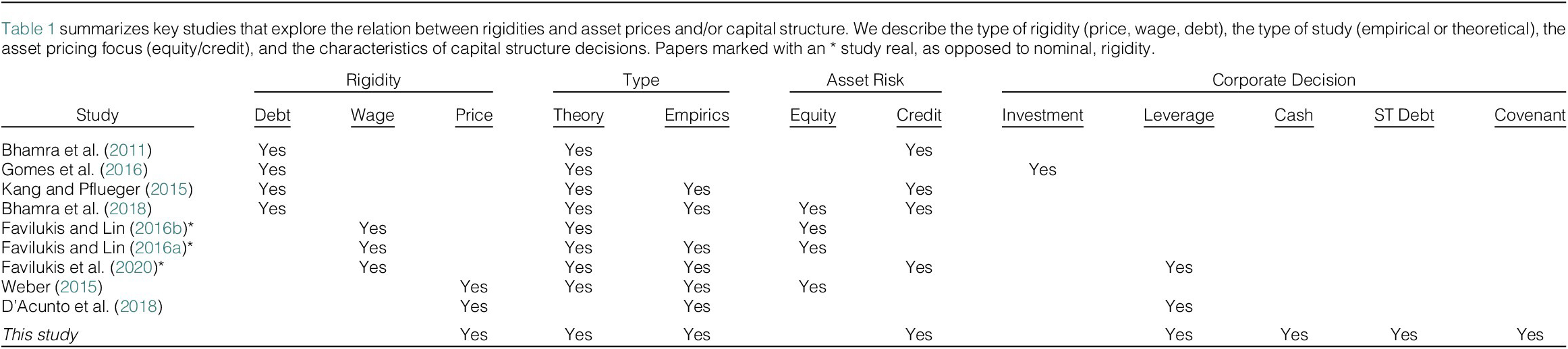
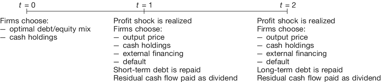


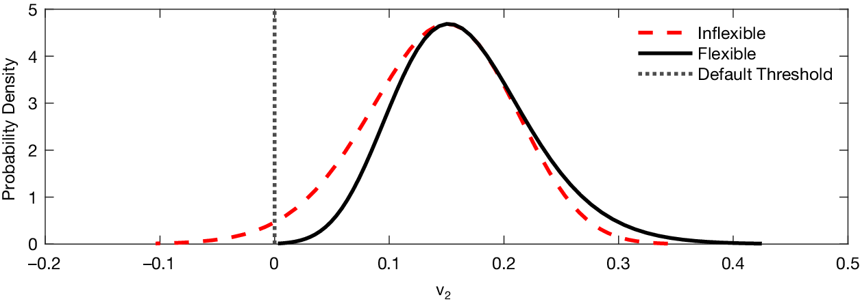


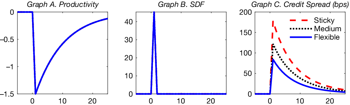


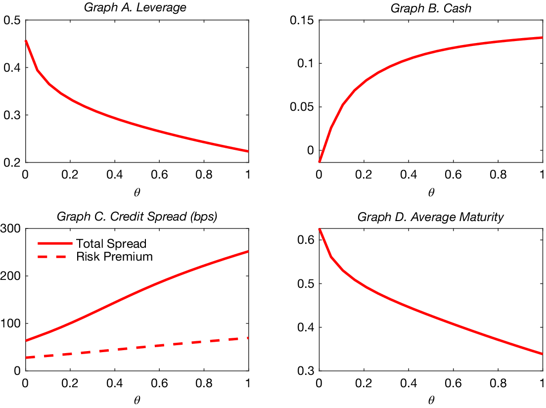


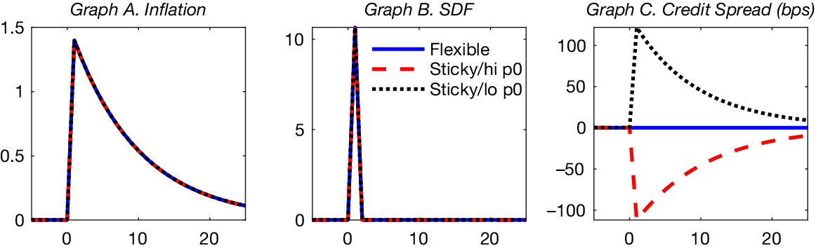


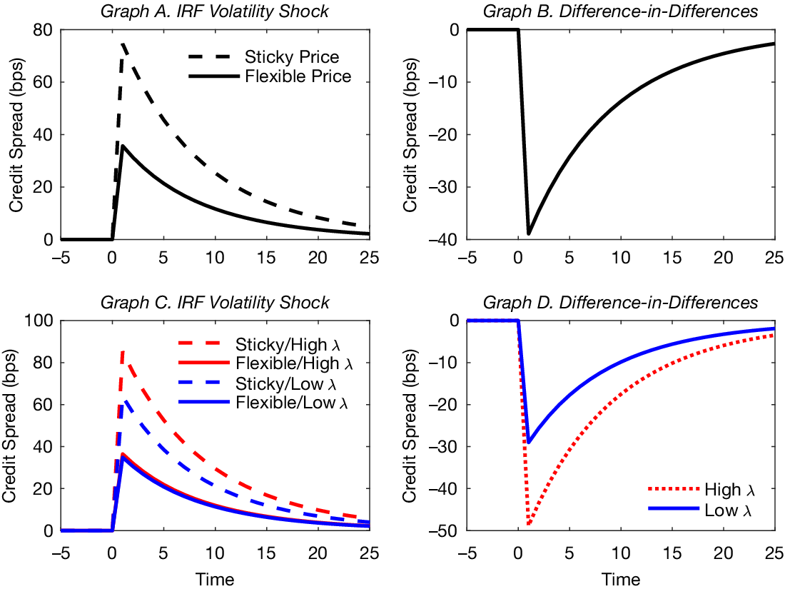


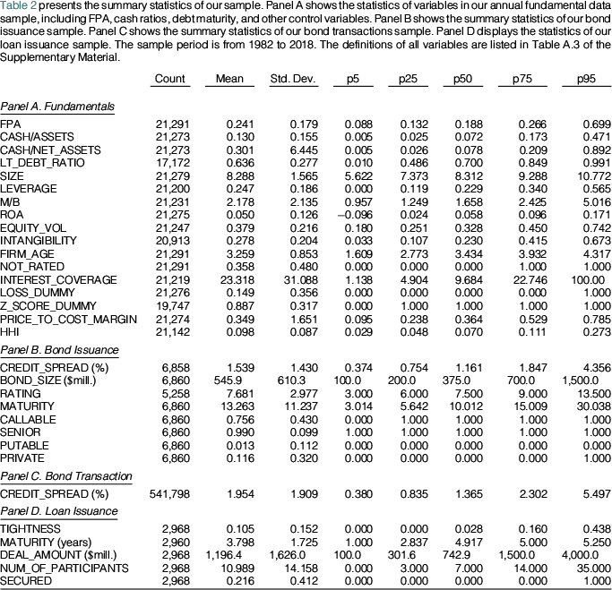
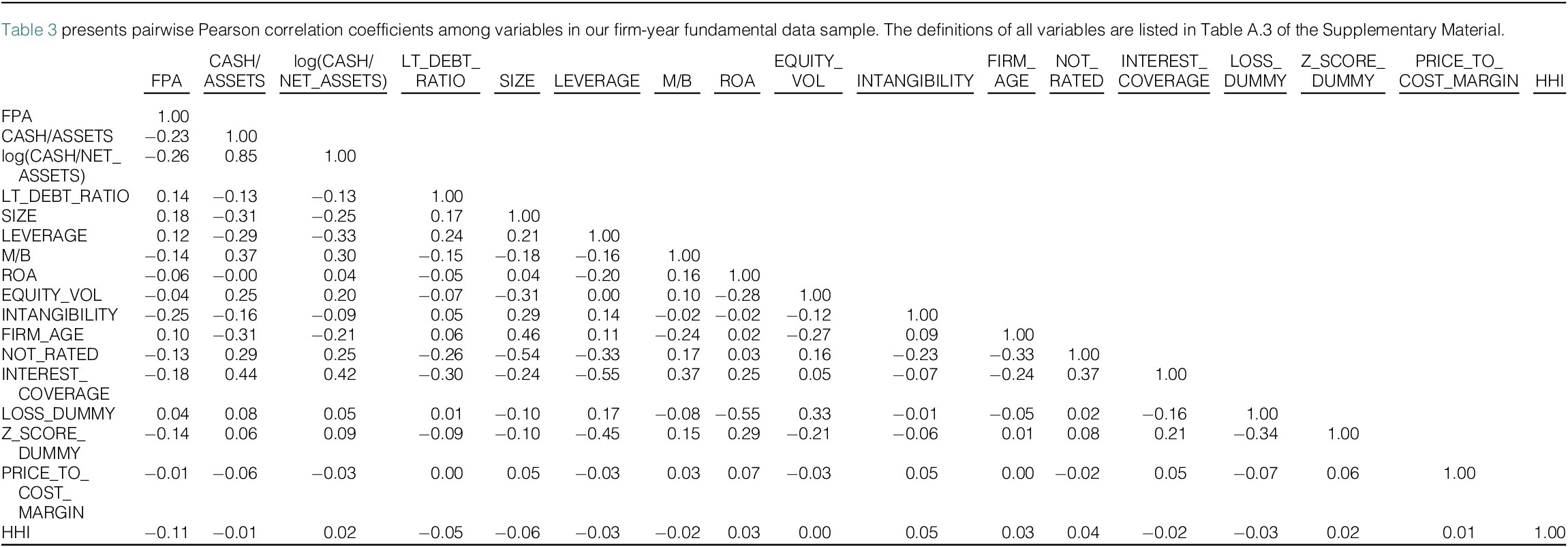
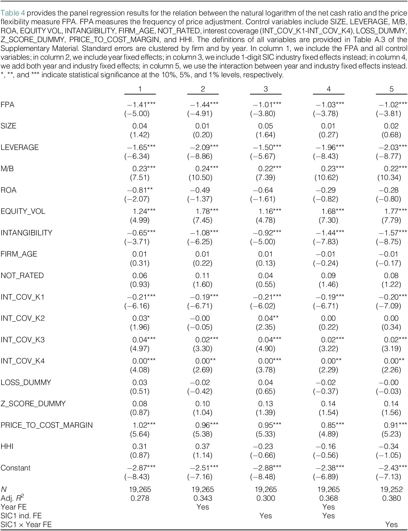
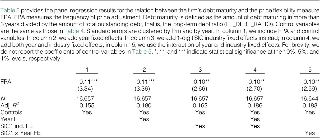
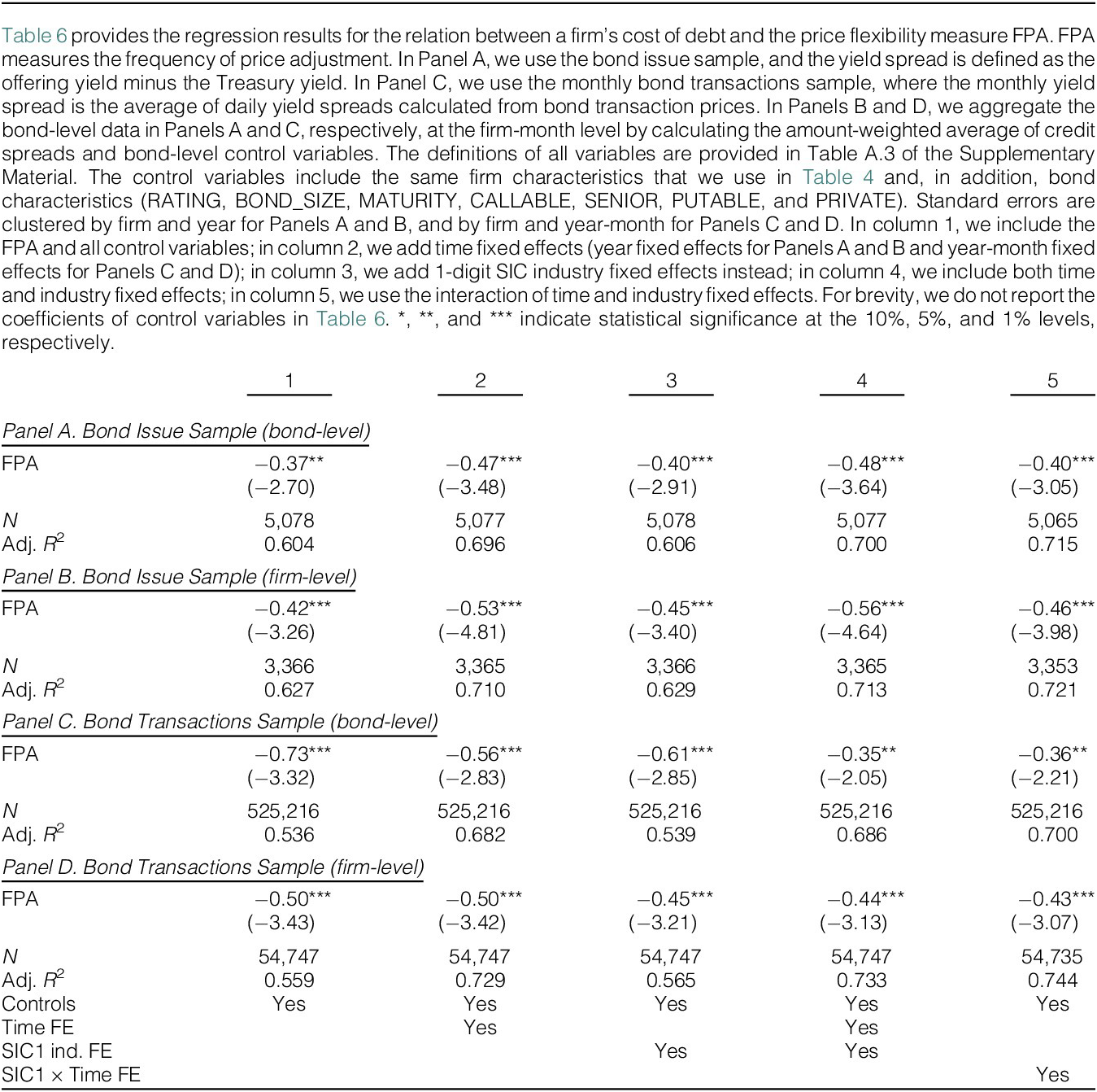
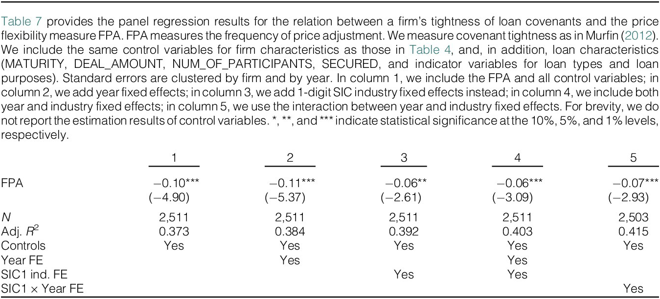
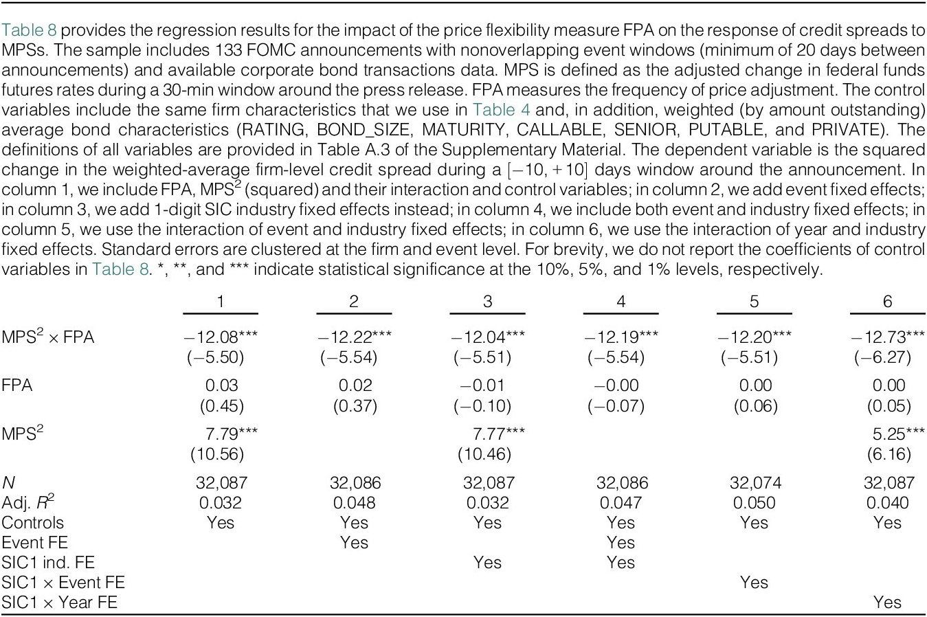
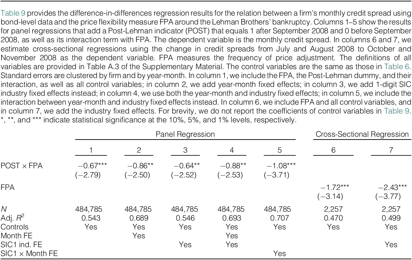
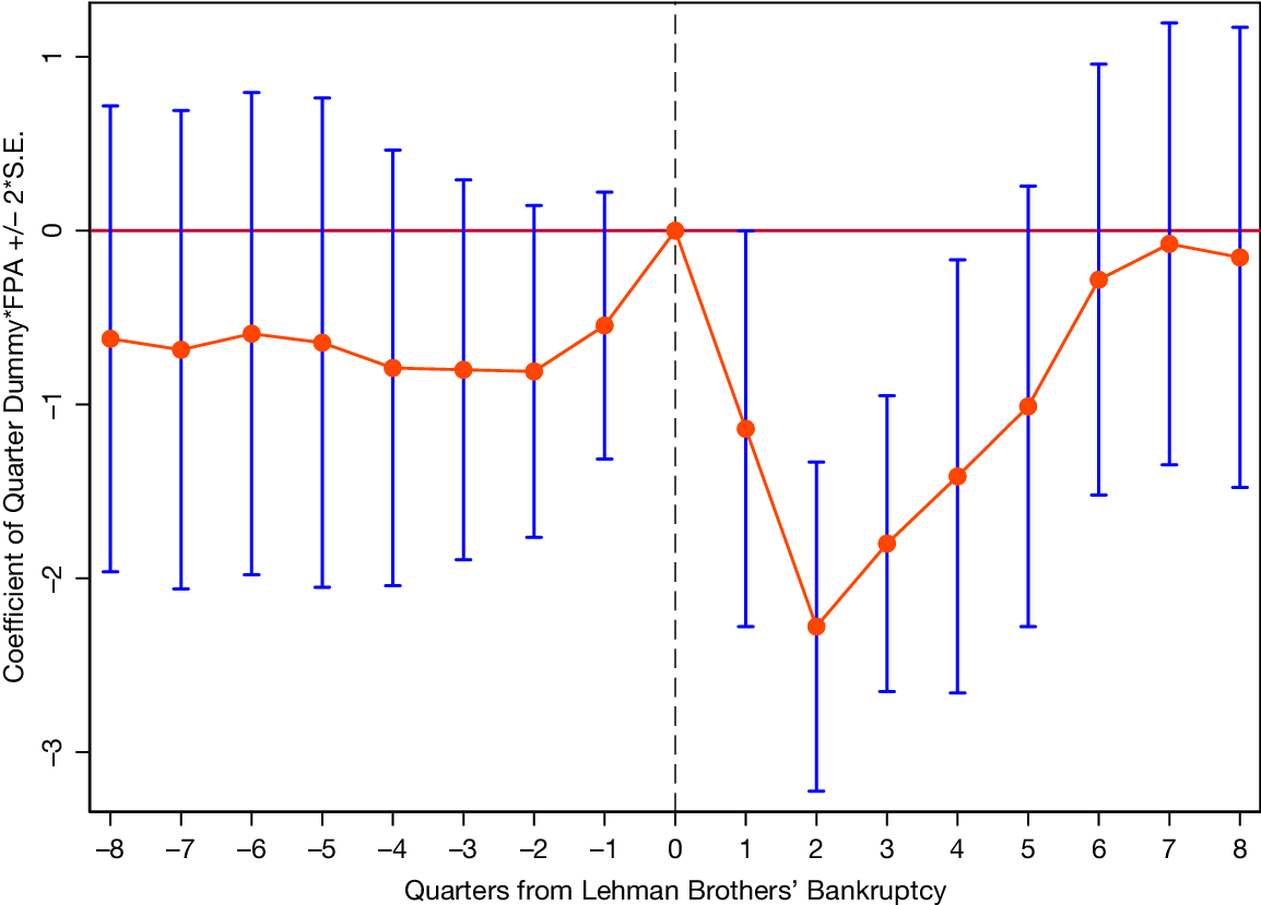


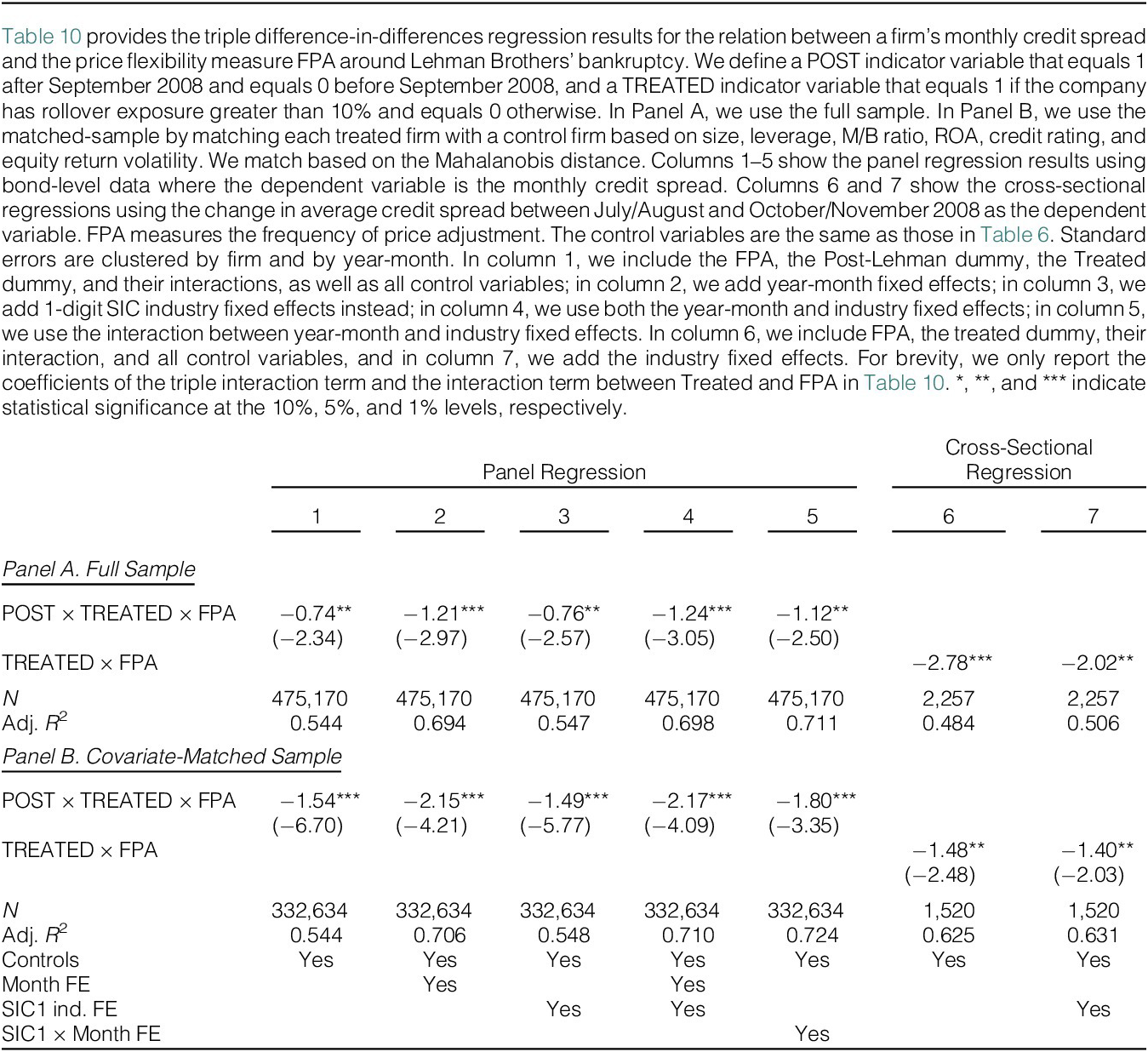


 Open access

