


Introduction
Continental precipitation and temperature patterns will most likely evolve with global climate change, influencing the environment of all living organisms on land, humans included. How precipitation and temperature patterns have evolved in the past remain poorly defined, and what forcing lead to pattern changes remain poorly understood, limiting adaption and mitigation strategies, as well as paleoenvironmental and geoarchaeological perspectives. Quantitative and semiquantitative proxy records of temperature and precipitation estimates across continental surfaces and at a high spatio-temporal resolution, ideally over longer periods (e.g., glacial–interglacial cycles) need to be retrieved from geological archives. However, today, few such datasets are documented for continental settings, and most are based on geochemical proxies, including δ13C and δ18O of biogenic calcite (Prud’homme et al., Reference Prud’homme, Fischer, Jöris, Gromov, Vinnepand, Hatté, Vonhof, Moine, Vött and Fitzsimmons2022), clumped isotopes from pedogenic carbonates (Újvári et al., Reference Újvári, Schneider, Stevens, Rinyu, Ilona Kiss, Buylaert and Sean Murray2024), and δ13C of organic matter (Hatté et al., Reference Hatté, Fontugne, Rousseau, Antoine, Zöller, Laborde and Bentaleb1998; Vinnepand et al., Reference Vinnepand, Fischer, Fitzsimmons, Thornton, Fiedler and Vött2020) recovered from loess deposits, a widespread continental geoarchive. Such analyses are rather costly and labor intensive and they cannot be necessarily performed universally (e.g., in the absence of bio-/pedogenic carbonates), limiting their extensive application.
Archives of climatic and environmental change inclusive of loess–paleosol sequences (LPS), which cover more than 10% of Earth’s land surface (Pye, Reference Pye1995), are available, however we lack well-tested and established tools to determine climate parameters in a cost- and labor-efficient way. Such tools would facilitate achieving the objective of high spatiotemporal resolution for tracing changes in climate patterns across continents. Recently, geophysical measures that traditionally have not been used in the loess community have gained increasing attention as alternative measures for temperature and precipitation reconstructions. Relevant measures include, but are not limited to (wavelength-specific) photo spectrometric data analyses (Laag et al., Reference Laag, Lagroix, Kreutzer, Chapkanski, Zeeden and Guyodo2023), frequency dependence (Δχ) of magnetic susceptibility (χ) (Maher et al., Reference Maher, Alekseev and Alekseeva2003; Liu et al., Reference Liu, Roberts, Larrasoaña, Banerjee, Guyodo, Tauxe and Oldfield2012; Schneider et al., Reference Schneider, Almqvist, Svedlindh, Hedlund, Thyr, Kurbanov and Stevens2025), and estimated maghemite contribution from thermomagnetic susceptibility (χtd) curves (Gao et al., Reference Gao, Hao, Oldfield, Bloemendal, Deng, Wang and Song2019). All of these measures aim at isolating the signal of climate sensitive (magnetic-) mineralogy of soils and sediments and are rather cost efficient. Therefore, they are promising proxies as complements to available geochemical proxies.
During the last three decades, various studies have been performed on LPS with the objective to establish such quantitative relationships (e.g., Maher and Thompson, Reference Maher and Thompson1995; Balsam et al., Reference Balsam, Ellwood, Ji, Williams, Long and El Hassani2011; Maher, Reference Maher2011; Bradák et al., Reference Bradák, Seto, Stevens, Újvári, Fehér and Költringer2021; Jordanova and Jordanova, Reference Jordanova and Jordanova2021). Various rock magnetic parameters, primarily from topsoils developing on loess, have been tested against climate variables, notably present day mean annual precipitation (MAP) and mean annual temperature (MAT). Generally, χlf is suggested to be enhanced during pedogenesis through the formation of magnetite and maghemite (Maher and Thompson, Reference Maher and Thompson1992; Balsam et al., Reference Balsam, Ellwood, Ji, Williams, Long and El Hassani2011; Buggle et al., Reference Buggle, Hambach, Müller, Zöller, Marković and Glaser2014). Recently, Gao et al. (Reference Gao, Hao, Oldfield, Bloemendal, Deng, Wang and Song2019) attempted to isolate the contribution of pedogenic maghemite from soils developing on loess of the Chinese Loess Plateau from susceptibility thermomagnetic curves to establish a transfer function to MAP. Laag (Reference Laag2023) tested the results of Gao et al. (Reference Gao, Hao, Oldfield, Bloemendal, Deng, Wang and Song2019) on the Suhia Kladenetz loess profile within the framework of doctoral thesis research.
Although temperature reconstructions based on rock magnetic properties have been attempted (e.g., Maher et al., Reference Maher, Alekseev and Alekseeva2003), these are generally less clear than the relationship between MAP and χlf (Han et al., Reference Han, Lü, Wu and Guo1996; Radaković et al., Reference Radaković, Gavrilov, Hambach, Schaetzl, Tošić, Ninkov, Vasin and Marković2019). In addition, MAP and MAT are strongly correlated in some areas (Han et al., Reference Han, Lü, Wu and Guo1996), leading to ambiguity as to which climatic properties actually cause variations in χlf. It should also be noted that variations in χ of LPS have been related to wind vigor effects (Begét and Hawkins, Reference Begét and Hawkins1989; Evans, Reference Evans1999; Evans and Heller, Reference Evans and Heller2003; Bradák et al., Reference Bradák, Seto, Stevens, Újvári, Fehér and Költringer2021; Vinnepand et al., Reference Vinnepand, Fischer, Hambach, Jöris, Craig, Zeeden and Thornton2023) and may be affected by dissolution of metastable magnetic minerals (Maher, Reference Maher1986; Nawrocki et al., Reference Nawrocki, Wøjcik and Bogucki1996; Evans and Heller, Reference Evans and Heller2003). Dissolution of magnetic minerals has been observed in many Western and Central European LPS under the influence of moist Atlantic airmasses (cf., Baumgart et al., Reference Baumgart, Hambach, Meszner and Faust2013, and references therein) or related to permafrost (Lagroix and Banerjee, Reference Lagroix and Banerjee2004; Taylor and Lagroix, Reference Taylor and Lagroix2015). In contrast, high coercivity and climate-sensitive magnetic minerals such as hematite and goethite may persist in rather moist environments (Kämpf and Schwertmann, Reference Kämpf and Schwertmann1983; Trolard and Tardy, Reference Trolard and Tardy1987; Retallack, Reference Retallack2001; Laag, Reference Laag2023; Laag et al., Reference Laag, Lagroix, Kreutzer, Chapkanski, Zeeden and Guyodo2023).
The concentrations of goethite and hematite are difficult to quantify in bulk sediment by standard magnetic measures in the presence of magnetite due to their low saturation magnetization (0.4 Am2/kg (hematite), <1 Am2/kg (goethite), 90–92 Am2/kg (magnetite) at room temperature) (Hunt et al., Reference Hunt, Moskowitz, Banerjee and Ahrens1995). Since even low amounts of Fe (hydr-) oxides in sediments are capable of strongly influencing the sediment/soil color (e.g., Lukić et al., Reference Lukić, Radaković, Marković, Thompson, Micić Ponjiger, Basarin and Tomić2023), colorimetric measures may provide meaningful quick and cost-efficient ways to derive semi-quantitative estimations of hematite and goethite concentration (Scheinost and Schwertmann, Reference Scheinost and Schwertmann1999; Balsam et al., Reference Balsam, Ji and Chen2004; Laag, Reference Laag2023; Laag et al., Reference Laag, Lagroix, Kreutzer, Chapkanski, Zeeden and Guyodo2023). Consequently, transfer functions have been established to estimate the abundance of various iron (hydr-) oxides from whole color spectra (using CIE-Yxy, CIE-L*a*b*, and Munsell systems) (Scheinost and Schwertmann, Reference Scheinost and Schwertmann1999; Laag, Reference Laag2023; Laag et al., Reference Laag, Lagroix, Kreutzer, Chapkanski, Zeeden and Guyodo2023). Hematite favorably forms in environments that are characterized by high temperatures and short periods of limited rainfall, which often prevail in warm, semi-arid and arid areas with a certain seasonality (Maher, Reference Maher1986; Balsam et al., Reference Balsam, Ji and Chen2004). In contrast, goethite preferably forms under relatively lower temperatures and considerably higher, less seasonal precipitation amounts. Higher organic carbon content, lower pH, and increased Al concentration also favor goethite precipitation and limit hematite formation (Schwertmann and Taylor, Reference Schwertmann, Taylor, Dixon and Weed2018). Direct extraction of the mineral-specific wavelengths from spectral data of geo-archives revealed promising results that are a good fit with past climatic features (Laag, Reference Laag2023). However, this relationship has not been tested in experiments across climate gradients.
Although this study focusses on the relationships between climate parameters and geophysical soil/sediment properties, other factors need to be considered, including the properties of the soil substrate and the accumulation rate of dust, which potentially play a role in the relationship between geophysical soil properties and climate (Porter et al., Reference Porter, Hallet, Wu and An2001; Maher et al., Reference Maher, Alekseev and Alekseeva2002), and inhomogeneous conditions that are expected to complicate the relationship. To account for this aspect, we exclusively used samples from Chernozems at the Bačka Loess Plateau (BLP) in Serbia. In addition, we performed a multivariate principal component analysis (PCA) in which we integrated log-transformed (ln) geochemical ratios (LOG Si/Al, LOG Ti/Zr) that indicate substrate inhomogeneities next to other climate-sensitive proxies (cf., approach used by Vinnepand et al., Reference Vinnepand, Fischer, Jöris, Hambach, Zeeden, Schulte and Fitzsimmons2022). After this initial check, we tested the relationship between measured climate parameters, such as MAP and MAT, with single geophysical parameters of modern topsoil samples (n = 50) taken along a precipitation gradient across the BLP.
In contrast to most of Asia, temperature and precipitation follow independent spatial patterns in the region of the BLP. We also tested the correlation between climate parameters (MAP; MAT) and aridity using the De Martonne (Reference De Martonne1925) Aridity Index (DMAI), which can be represented as following equation:
 \begin{equation}{\textit{DMAI = }}\frac{{{\textit{MAP}}}}{{{\textit{MAT + C}}}}\end{equation}
where, MAP is the annual amount of precipitation in mm, MAT is the mean annual surface air temperature in °C, and C = 10°C is the De Martonne’s constant (De Martonne, Reference De Martonne1925).
We additionally compared MAP, MAT, and DMAI to proxy combinations in multi-regression analyses considering proxies that can be frequently determined in laboratories available for the loess community, as well as more specific magnetic proxies that may require more sophisticated analytical equipment. We performed these regression analyses to test if climate parameters can be explained better through linear combination of our multi-proxy dataset relative to comparisons between single proxies to these parameters.
In a last step, we performed linear regression analyses considering the PCA outputs that can be applied to the entire dataset to reduce the data dimension. Through this, we extracted the most relevant information from the dataset and compared this to climate parameters with a strongly reduced risk of overfitting.
Overall, we present a robust multi-proxy and multivariate statistical approach that tests the sensitivity of single geophysical parameters and combinations of these to small climate differences. We emphasize, for future works, that independent calibration may be required in other paleoclimatic and environmental settings in space and time. The present study focuses on topsoils developing on loess in order to benchmark results on available climate reconstructions. We used the same samples as Radaković et al. (Reference Radaković, Gavrilov, Hambach, Schaetzl, Tošić, Ninkov, Vasin and Marković2019), but largely extended the dataset to go from a single-proxy calibration to a multi-proxy study and to provide a table assessing the proxies for similar settings.
Regional setting and meteorological data
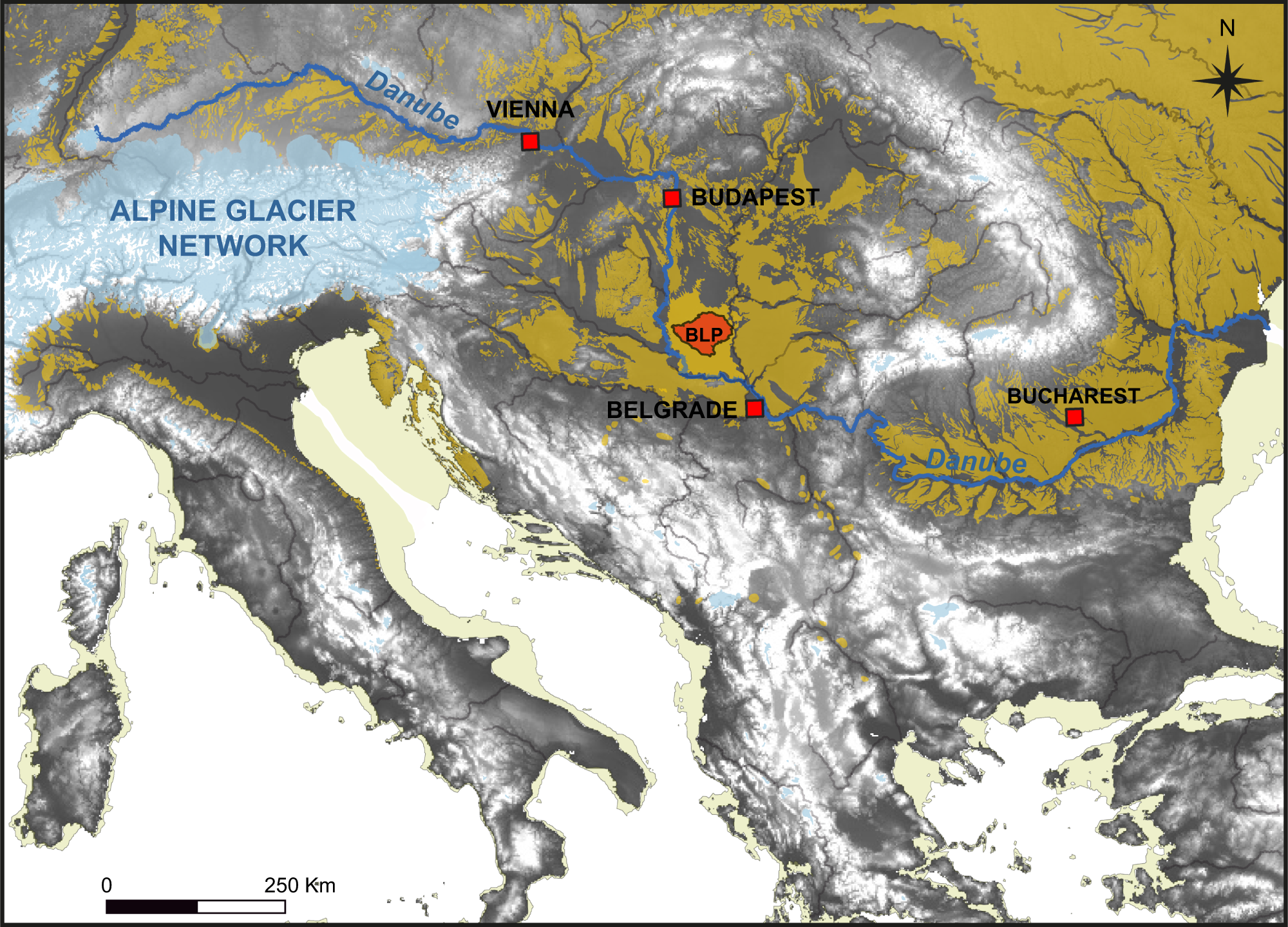
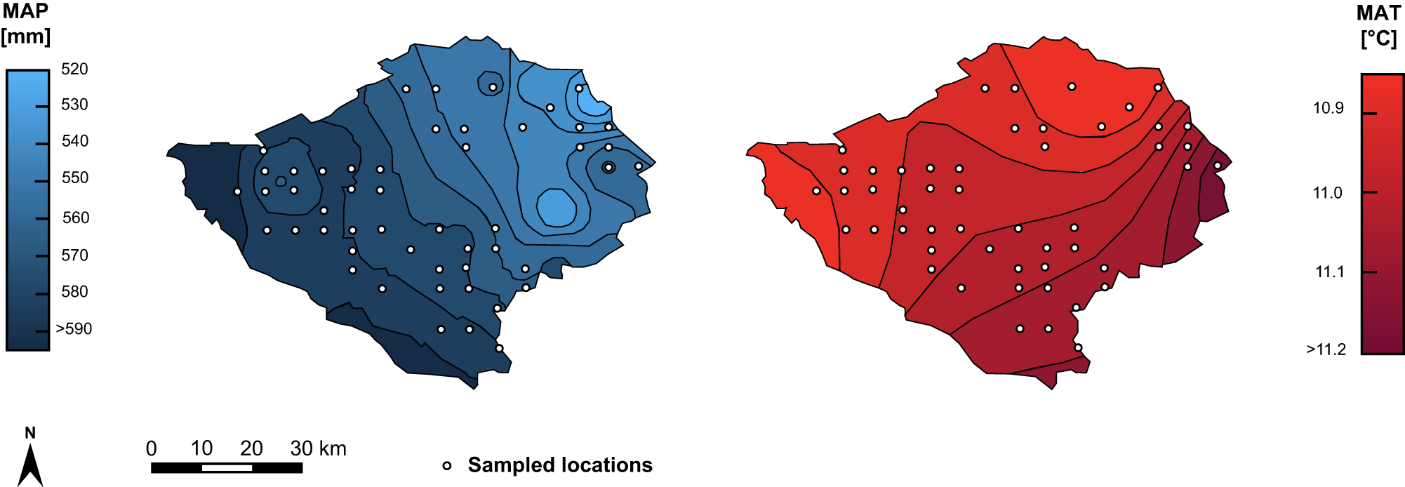
The Bačka Loess Plateau (BLP) is located in the southern part of the Middle Danube Basin, between the Danube stream to its west and south and the Tisza River to its east and spans an area of ∼2500 km2 (Fig. 1). Presumably, these river systems dissect a formerly larger loess-covered area to which the BLP contributed (Popov et al., Reference Popov, Marković and Štrbac2008). Although the dust sources of the BLP remain in discussion (Buggle et al., Reference Buggle, Glaser, Zöller, Hambach, Marković, Glaser and Gerasimenko2008; Marković et al., Reference Marković, Stevens, Kukla, Hambach, Fitzsimmons, Gibbard and Buggle2015), it is reasonable to assume a relatively homogenous mixture of dust material from the Danube and Tisza catchments and the surrounding mountainous areas as the main dust contributors (cf., Fenn et al., Reference Fenn, Millar, Durcan, Thomas, Banak, Marković, Veres and Stevens2022). The narrow MAP gradient, across the plateau, decreases from west (584±1 mm/yr) to east (525±1 mm/yr), while the very narrow MAT gradient is observed along a southeast (11.2±0.1 °C) to northwest (10.8±0.1 °C) axis (Fig. 2; Radaković et al., Reference Radaković, Gavrilov, Hambach, Schaetzl, Tošić, Ninkov, Vasin and Marković2019). Given that the observed temperature range (ΔMAT = 0.3 °C) is very close to the measuring error of 0.1 °C (cf., WMO, 1979), we did not perform regression analyses to derive temperature climo-functions based on the meteorological dataset at the BLP. Instead, we provide scatterplots that allow for an initial idea of the potential of MAT- geophysical-data relationships when a wider MAT range is considered.
Map based on a digital elevation model (GLOBE 1.0; WGS84) showing southeastern Europe during the last glacial maximum (LGM, centered at ca. 22 ka). The Bačka Loess Plateau (BLP, Serbia), is within the Middle Danube Basin. This special setting favored the accumulation of the oldest known LPS in Europe and supports a rather homogenous mineral dust assemblage in terms of provenance (Danube and Tisza catchment, local mountain ranges), which was favorable for our study. We checked the spatial substrate homogeneity across the BLP using XRF data to constrain any loess-provenance-related study bias. Loess distribution as outlined by Lehmkuhl et al. (Reference Lehmkuhl, Nett, Pötter, Schulte, Sprafke, Jary and Antoine2021); LGM ice extent from Ehlers and Gibbard, (Reference Ehlers and Gibbard2004).

Distribution of mean annual precipitation (MAP) and mean annual temperature (MAT) across the Bačka Loess Plateau (Serbia) (modified after Radaković et al., Reference Radaković, Gavrilov, Hambach, Schaetzl, Tošić, Ninkov, Vasin and Marković2019) derived from proximal meteorological stations (see supplement in Radaković et al., Reference Radaković, Gavrilov, Hambach, Schaetzl, Tošić, Ninkov, Vasin and Marković2019, for their exact locations). A narrow but measurable MAP gradient exists between the eastern and western parts of the loess plateau. The MAT gradient is close to the measuring error and generally follows a south–north direction. Both MAP and MAT are uncorrelated—a situation that seldomly prevails across Eurasia—favoring assessment of the effects of MAP versus MAT on multivariate geophysical parameters. These have been measured on 50 samples (white dots) across the plateau, complementing Radaković et al. (Reference Radaković, Gavrilov, Hambach, Schaetzl, Tošić, Ninkov, Vasin and Marković2019).

Our contribution focuses on precipitation differences across the BLP and how these are linearly expressed across the plateau along a narrow (ΔMAP = 59±1 mm/yr) precipitation gradient. Other studies worldwide confirm that the value-range in our study aligns with the range in which there is a significant relationship between magnetic susceptibility data and MAP (cf., Radaković et al., Reference Radaković, Gavrilov, Hambach, Schaetzl, Tošić, Ninkov, Vasin and Marković2019, fig. 7B, and references therein). Across the BLP, the existence of this narrow precipitation gradient occurs in a topographically flat landscape without any orogenic obstacles within the Carpathian Basin. Therefore, although narrow, a MAP range of 59±1 mm/yr makes a considerable difference in environmental conditions and the observed pattern is meaningful as the highest MAP values relative to the westernmost part of the BLP that is closest to the Mediterranean Sea.
In the framework of multi-regression analyses and PCA, we made use of the DMAI. The error of this index depends on the errors of both observed meteorological data (MAT and MAP) and on the aridity value itself. Because the errors of both MAP and MAT are constant, the error of DMAI values and its variation are also constant. Considering the range of MAP and MAT across the BLP, the DMAI error is ±0.025 mm/°C (see equations in the Supplement for details on the calculation of the DMAI error and the error on meteorological data).
Materials and methods
This study comprises 50 topsoil samples taken from the plough horizon of Chernozems across the BLP at a sampling depth of 10 cm (Radaković et al., Reference Radaković, Gavrilov, Hambach, Schaetzl, Tošić, Ninkov, Vasin and Marković2019). Since these fertile soils are under intensive agricultural land use (and/or have been in the past), an intensive mixing of the substrate and at least temporal exposure to the atmosphere can be reasonably assumed. This ensures that the geophysical properties of the soil material align with recent climatic conditions. Fertilizers are capable of influencing magnetic properties of topsoils—especially in soils that experience intensive agricultural activity (da Silva et al., Reference Da Silva, Triantafyllou and Delmelle2023). All samples were taken after the harvest from areas without spring fertilization for fertility control (i.e., if there was any autumn fertilization, approximately nine months had passed when sampling took place). Therefore, no short-term fertilizer effects are expected that could influence the magnetic properties of our samples.
Long-term effects are more difficult to assess because no data are available that document the exact type and quantity of applied fertilizers across the BLP over a longer period. Frequently applied phosphorous fertilizers appear to have no obvious effect. When applying regression analyses for samples that fall within the natural background for the Vojvodina region (up to ∼20 ppm), no meaningful linear relationship can be observed between P2O5 and MAP or between P2O5 and all considered magnetic parameters. This applies also for samples exceeding this threshold (Supplements S1, S2). Thus, there is no obvious effect of P-containing fertilizers on the magnetic mineralogy across the BLP that would bias our study.
Considering the outlined conditions and sampling practice, we regard our approach as the best possible basis for the performance of our study apart from laboratory experiments that are limited by the duration of pedogenic processes. All samples were taken in areas where the influence of intensive industry, traffic, settlements, gullies, and freshwater ecosystems can be regarded to be as minimal as possible. After drying (air-drying) and sieving (2 mm), the samples were carefully stuffed into plastic boxes (prevention of particle movement), resulting in 6.4 cm3 samples. For hysteresis measurements, approximately 400 mg of sample material was filled into non-magnetic gelatine capsules, which were sealed with temperature-resistant tape. The net mass of sample material was determined before filling and all resulting mass-dependent values were mass normalized.
Environmental magnetic proxies
Magnetic susceptibility and its frequency dependency
The volume-specific magnetic susceptibility (χ), although frequently applied in loess research, is a composite signal because all materials in a sample contribute. Due to their intrinsically high χ, low concentrations of ferromagnetic minerals such as magnetite (pedogenic and diagenetic) and maghemite (pedogenic) will dominate composite χ values (Liu et al., Reference Liu, Roberts, Larrasoaña, Banerjee, Guyodo, Tauxe and Oldfield2012). We determined χ using a susceptibility bridge (VFSM; Magnon, Germany) at AC fields of 505 Hz and 5050 Hz with a field amplitude of 400 A/m. Measurements were normalized for the sample mass thus low-field, low-frequency χ is referred to as χlf; low-field and high frequency χ is referred to χhf hereafter. The frequency dependence of magnetic susceptibility is considered as the absolute difference between χlf (505 Hz) and χ hf (5050 Hz) and is thus named Δχ here.
 \begin{equation}{\Delta \chi = \chi lf } - {\chi hf }\end{equation}
For comparison, we also provide the percentage of frequency dependence of magnetic susceptibility:
 \begin{equation}{\Delta \chi [\% ] = }\frac{{{\Delta \chi }}}{{{\chi lf}}}{{ \times 100}}\end{equation}
Δχ provides information on the proportion of the composite signal resulting from superparamagnetic (SP) particles (< ∼20–27 nm at room temperature) (Moskowitz et al., Reference Moskowitz, Frankel, Walton, Dickson, Wong, Douglas and Mann1997), which has been demonstrated to being primarily of pedogenic origin in soils developing on loess (Maher and Thompson, Reference Maher and Thompson1992). If SP particles are created during pedogenesis both Δχ and in χlf will increase proportionally. In the wind vigor model, where coarser (non SP) magnetic particles would be preferentially deposited, χlf would increase inducing no change in Δχ. In post-depositional processes leading to dissolution of ferrous iron oxides (i.e., magnetite), the finest particles would be preferentially dissolved first, leading to a decrease of both Δχ and χlf with a greater effect on Δχ. Thus, comparing Δχ to χlf may provide information on the nature of the variation observed in magnetic susceptibility values.
Maghemite contribution to high-temperature variations of magnetic susceptibility
High temperature thermomagnetic experiments were conducted, under Ar supply, using a MFK1-FA AGICO Kappabridge operating with a 400 A/m and 976 Hz alternating field. Maghemite concentrations were deduced from these experiments based on the postulate that maghemite, a ferric iron oxide, in our samples is primarily of pedogenic origin resulting from the partial or complete oxidation of magnetite. Upon heating, maghemite, which is known to be metastable, may convert to hematite at temperatures as low as ∼250 °C (Gehring et al., Reference Gehring, Fischer, Louvel, Kunze and Weidler2009) and as high as 500 °C (Özdemir and Banerjee, Reference Özdemir and Banerjee1984). Gao et al. (Reference Gao, Hao, Oldfield, Bloemendal, Deng, Wang and Song2019) proposed and demonstrated that maghemite concentrations may be estimated from the difference between χlf at 230 °C and 400 °C in the heating curve of thermomagnetic experiments (Gao et al., Reference Gao, Hao, Oldfield, Bloemendal, Deng, Wang and Song2019, fig. 4B). They further demonstrated a strong correlation between the estimated maghemite contents and MAP across the Chinese Loess Plateau and developed a magnetic-susceptibility-based climo-function for quantifying paleoprecipitation. It should be noted that not all “humps” in a thermomagnetic curve result from mineral conversion. On heating, a population of stable single-domain particles transitioning to a superparamagnetic state will result in magnetic susceptibility increasing and decreasing, producing a hump as shown in the study of Zhang and Appel (Reference Zhang and Appel2023) on a basalt sample. A shift in temperature of the hump on cooling, leading to irreversibility, can be the result of a change in grainsize of the particle population and not be related to mineral transformation. Thus, we advise a careful evaluation of thermomagnetic experiments prior to estimating maghemite content following the method of Gao et al. (Reference Gao, Hao, Oldfield, Bloemendal, Deng, Wang and Song2019). In using the fraction of χlf that can be assigned to pedogenic maghemite, instead of the bulk χlf, we excluded the diagenetic background (provenance) information from our analyses.
Anhysteretic remanent magnetization (ARM)
Stable single-domain and larger magnetic minerals exhibit the ability to retain a magnetic remanence, such as the anhysteretic remanent magnetization (ARM) (Liu et al., Reference Liu, Roberts, Larrasoaña, Banerjee, Guyodo, Tauxe and Oldfield2012, and references therein). For a given particle, the strength of the acquired remanence in a given magnetic field (geomagnetic or laboratory produced) is size- (magnetic domain) dependent (Peters and Dekkers, Reference Peters and Dekkers2003). In this study, ARM was induced by using a Magnon International AFD 300 in a peak AF field of 100 mT superimposed by a 0.1 mT DC field. Acquired ARM values were measured using a 2G enterprises 760 SRM magnetometer.
Hysteresis experiments
Hysteresis measurements are not routinely undertaken in loess research because they require more sophisticated analytical tools and expertise. Despite this, they are favorable compared to many geochemical applications, considering their efficiency in terms of measurement time and costs and the possibility of producing multi-proxy datasets. All hysteresis measurements were conducted using a Princeton Measurements Corporation Model 3900 Vibrating Sample Magnetometer (VSM) at the Institut de Physique du Globe de Paris (CNRS/IPGP/Université Paris Cité). Hysteresis loops were acquired in maximum applied fields of ± 1.5 T with a constant 5 mT field increment and averaging the measured moment at each step for 100 ms. All experiments started at the positive maximum field following a 1s pause. From each hysteresis loop, we derived the following mass-normalized magnetic parameters:
χhifi—The magnetic susceptibility derived from the slope of the loop at high field (χhifi) over the field range of 1050–1500 mT. Minerals contributing to χhifi are paramagnetic, diamagnetic, and non-saturated ferromagnetic minerals (e.g., goethite). Ferrimagnetic minerals, such as magnetite and maghemite, saturate at lower fields and therefore to do not contribute to χhifi. With respect to hematite, its antiferromagnetic component generally will not be saturated and will contribute to χhifi, while its weak ferromagnetic component, as particle size increases, can saturate in lower fields than considered for χhifi (Özdemir and Dunlop, Reference Özdemir and Dunlop2014).
χferri—Ferrimagnetic susceptibility (χferri) is derived by subtracting, for a given sample, χhifi from the bulk χlf, thus isolating predominantly the contribution of magnetite and maghemite. In this study, bulk χlf was measured on the same sample prior to the start of hysteresis measurements using an AGICO KLY-3 Kappabridge operating in a 300 A/m applied field at a frequency of 875 Hz and calculated χferri:
 \begin{equation}\chi ferri\text{ }=\text{ }\chi_{lf}\left(KLY-3\right)\text{ }-\text{ }\chi hifi\end{equation}
(Saturation) remanence magnetization (Mrs and Mr)—The magnetization remaining when the field is reduced to zero after starting in a saturating field is called saturation remanence magnetization (Mrs). When conducting a hysteresis experiment, if the hysteresis loop is not closed by the maximum field applied, the magnetization observed when the field is reduced to zero is simply a remanence magnetization (Mr) and more specifically an isothermal remanent magnetization (IRM), which is acquired at a set stable temperature.
Saturation magnetization (Ms)—In the hysteresis experiments conducted, the saturation magnetization (i.e., the magnetization at which increasing the external applied field no longer induces a change in magnetization) was derived from the high field slope-corrected hysteresis loops. For a given magnetic mineral, Ms is an intrinsic physical property and is independent of its magnetic grainsize. It is thus considered to be a very good normalizer in developing proxy ratios.
Coercivity (Hc)—The coercivity (Hc) in a magnetic mineral assemblage is the field strength that is necessary to drive a magnetization from saturation to zero. Increased Hc values may relate to the presence of magnetic minerals with high saturation levels such as hematite and goethite (Liu et al., Reference Liu, Roberts, Larrasoaña, Banerjee, Guyodo, Tauxe and Oldfield2012).
Coercivity of Remanence (Hcr)—The coercivity of remanence depends on the magnetic grainsize and defines the field strength necessary to reduce the saturation remanence magnetization to zero. A separate experiment was conducted to determine Hcr where the sample was subjected to a +1.5 T saturation field. The acquired Mrs was subsequently subjected to backfields incrementally increasing from zero to −0.5 T in 70 logarithmically spaced intervals.
S-ratio and HIRM—The S-ratio and HIRM are valuable parameters to estimate the relative concentrations of soft (low-coercivity) and hard (high-coercivity) magnetic minerals. The same experiment conducted to determine Hcr was followed by modifying the backfield increment to a linear 100 mT interval over the 0 to −1.5 T range.
The hard isothermal remanent magnetization (HIRM) provides an absolute value of the remanence mobilized after saturation within the backfield range of −0.3 T and 1.5 T attributed to high coercivity magnetic minerals such as hematite and goethite. HIRM is calculated following (Taylor and Lagroix, Reference Taylor and Lagroix2015) from:
 \begin{equation}HIRM{\text{ }} = {\text{ }}IRM{-_{0.3T}}-{\text{ }}IRM{-_{1.5T}}\end{equation}
The S-ratio is a parameter that may be used to estimate the relative contribution to the total remanence of high-coercivity minerals (e.g., goethite and hematite) in a mixture with low-coercivity minerals (e.g., magnetite, maghemite). When the S ratio is close to 1, low-coercivity minerals dominate the mineral assemblage. Because the relative abundance of high-coercivity hematite and goethite increases, the S-ratio decreases (Liu et al., Reference Liu, Roberts, Larrasoaña, Banerjee, Guyodo, Tauxe and Oldfield2012). However, it is important to note that the interpretation of S-ratio depends on the experimental settings (strength of fields applied), which relates to the relative proportion of remanence carried above and below a certain threshold. These relative proportions of remanence do not equate to abundances of masses. For the later point Frank and Nowaczyk (Reference Frank and Nowaczyk2008) provided a good illustration. In the present study, the S-ratio was determined following the formula of King and Channell (Reference King and Channell1991):
 \begin{equation}S - ratio = \frac{{IRM - 0.3T}}{{IRM-1.5T}}\end{equation}
Colorimetric analyses for goethite and hematite determination
The color of sediments is a powerful tool to estimate the mineralogical composition of samples in terms of Fe-oxide quantities that exhibit a distinct color characteristic (Scheinost and Schwertmann, Reference Scheinost and Schwertmann1999). Hematite and goethite are viable targets for such an approach because they have clearly separable colorimetric wavelength-spectra (hematite: 510–560 nm; goethite: 410–460 nm) facilitating the isolation of their colorimetric signal hence their occurrence in a sample and deriving a concentration (Laag, Reference Laag2023; Laag et al., Reference Laag, Lagroix, Kreutzer, Chapkanski, Zeeden and Guyodo2023). High concentration of hematite indicates high temperatures and marked seasonality, whereas the occurrence of goethite is associated with higher excess in moisture, organic carbon content of the substrate, and lower pH (Kämpf and Schwertmann, Reference Kämpf and Schwertmann1983). Both iron (hydr-) oxides form predominantly during pedogenesis and their relative abundance (goethite over hematite ratio) is related to moisture availability, and other factors such as temperature, pH, and Al-concentration (Cornell and Schwertmann, Reference Cornell and Schwertmann2003).
To quantify hematite and goethite (see Laag, Reference Laag2023; Laag et al., Reference Laag, Lagroix, Kreutzer, Chapkanski, Zeeden and Guyodo2023) and to include the color data into linear modeling, we performed colorimetric measurements using a Konica Minolta CM600d spectrophotometer, averaging five measurements that had been conducted directly on bare homogeneous raw material. For this, ∼20 g of sample material was placed on a white paper and compressed to achieve a flat and homogenous surface. Prior to each measurement the spectrometer was calibrated using a black and white standard (provided by Konica Minolta).
The extraction of semi-quantitative goethite and hematite concentration data was conducted following Laag et al. (Reference Laag, Lagroix, Kreutzer, Chapkanski, Zeeden and Guyodo2023) and involved following steps: (1) transformation of the diffuse reflectance spectroscopy values from reflectance to absorbance values via the Kubelka–Munk function,
 \begin{equation}F(R)= \frac{(1-R)^{2}}{2R}\end{equation}
in which R is the dimensionless relative reflectance output value from the Konica-Minolta instrument; (2) identification of the absolute and true band amplitude (TBA) and estimation of the semi-quantitative goethite and hematite contents (we calculated TBA from the absolute peak height in the second derivative of the Kubelka–Munk transformed absorbance of reflectance values); and (3) we identified the first minimum of the second derivative of the Kubelka–Munk recalculated absorbance of reflectance data for goethite between 410 nm and 430 nm and the maximum between 440 nm and 460 nm. For hematite the first minimum between 510 nm and 530 nm and the maximum between 550 nm and 580 nm was considered. To calculate semi-quantitative amounts of goethite and hematite, we used the absolute difference of these reflectance values in the ordinate of the second derivative of the DRS data (Laag, Reference Laag2023; Laag et al., Reference Laag, Lagroix, Kreutzer, Chapkanski, Zeeden and Guyodo2023, and references therein).
X-ray fluorescence (XRF) analyses to test the effect of provenance changes
We performed multi-element analyses using the Bruker Tracer 5g portable energy-dispersive XRF device with the GeoExploration calibration, with three phases and a total time measurement of 120 s. These measurements were made on sieved (< 2 mm), ball-milled (5 min, 450 rounds/min) samples (n = 50) to create logarithmic (ln) element ratios sensitive for provenance changes and grainsize sorting (LOG Si/Al, LOG Ti/Zr) and decalcification, secondary carbonate re-precipitation (LOG Ca/Fe) (cf., Vinnepand et al., Reference Vinnepand, Fischer, Jöris, Hambach, Zeeden, Schulte and Fitzsimmons2022, Reference Vinnepand, Fischer, Hambach, Jöris, Craig, Zeeden and Thornton2023). We are fully aware that handheld XRF devices and their calibration should be considered with caution (Da Silva et al., Reference Da Silva, Triantafyllou and Delmelle2023) and we understand the data variance as a good first estimation of provenance and grainsize shift patterns and decalcification. In the western Central European Schwalbenberg key loess section (Germany) the trends in the LOG Ca/Fe and LOG Ti/Zr ratios between handheld (NITON GOLDD 5000, Soil mode) and stationary XRF measurements (polarization energy dispersive X-ray fluorescence (EDP-XRF) spectrometer (Spectro Xepos, Spectro) yielded striking similarities. Large shifts in all mentioned provenance and grainsize parameters are absent between the sites across the BLP, suggesting a rather uniform homogenized loess substrate. In contrast, the LOG Ca/Fe rate decreases with increasing precipitation.
Granulometric measures
For integrating grainsize data into our initial PCA to check for provenance, substrate inhomogeneity, and weathering-related effects, we performed granulometric measures. This involved the application of the protocol of Vlaminck et al. (Reference Vlaminck, Kehl, Lauer, Shahriari, Sharifi, Eckmeier, Lehndorff, Khormali and Frechen2016). Accordingly, we did not remove the inorganic and organic carbon fractions prior to grainsize analyses. Sample dispersion was achieved through mixing the sediment material with 1.25 ml of 0.1 M sodium pyrophosphate decahydrate (Na4P2O7 × 10H2O) for at least 12 hours in an overhead shaker (Blott and Pye, Reference Blott and Pye2008; Schulte et al., Reference Schulte, Lehmkuhl, Steininger, Loibl, Lockot, Protze, Fischer and Stauch2016). All particle size determinations were performed through a Beckman-Coulter LS 13320 PIDS Laser Diffraction Particle Size Analyzer providing grainsize classes that represent the mean diameter of particles over a size range of 0.04–2000 μm. The grainsize distribution was calculated applying Frauenhofer theory, but the number of clay-sized particles might be underestimated due to variations in the particle mineralogy and morphology (Beuselinck et al., Reference Beuselinck, Govers, Poesen, Degraer and Froyen1998).
Statistical data exploration
In our multivariate statistical approach, we tested selected geophysical proxies against climate data, geochemical indicators (provenance, substrate inhomogeneity, weathering), and grainsize variations. Classic linear correlation analyses using the Pearson correlation coefficient (r 2) (Pearson, Reference Pearson1895) are commonly applied, and we used this measure here.
Principal component analyses
A principal component analysis (PCA) is an established and robust method to detect the most important (rank-ordered) and separated (uncorrelated) drivers (principal components) in multivariate datasets that often come with variables that influence each other (Pearson, Reference Pearson1901; Jolliffe and Cadima, Reference Jolliffe and Cadima2016). Principal components can be compared directly to the original variables that have been integrated into the analyses to investigate how the specific proxy drives the principal components that frequently reflect processes/responses to environmental conditions. In our case, we used proxy data for PCA and compared the results of the PCA and the behavior of the original variables with the distribution of rainfall by applying a rank-ordered (by quantity of MAP) colorization of the sample points in the resulting PCA plots. Through this, it became apparent which proxy parameters best reflect precipitation distribution. All PCA analyses were performed using the ‘prcomp’ function in the ‘stats’ package of R (R Core Team, 2025).
Multidimensional regression analyses
To investigate the strengths of relationship between the physical parameters and climate, we performed regression analyses using the ‘lm’ function in the R software (R Core Team, 2025). Such analyses can be applied to a dependent variable and one or more explanatory variable(s) (Draper and Smith, Reference Draper and Smith1998). We carried out a multivariate regression to explore the possibility of explaining MAP, MAT, and aridity (DMAI) through linear combination of our multi-proxy dataset. To avoid overfitting, we also applied PCA and included PCA results (scores) in the model. Note that multivariate regression only considers linear combinations, which is thus limited. While it was possible to include more complex (e.g., logarithmic) relationships, for the sake of ensuring interpretability, a linear combination model was used.
Multidimensional regression on parameters that are frequently applied in loess research
To achieve an added value for large parts of the loess community, we created a linear regression between MAT, MAP, and DMAI and proxies that are traditionally and/or increasingly applied in loess research (χlf, Δχ, χtd, and ARM). In a second step, we compared this linear model to each climate parameter to evaluate the linear fit between both variables.
Multidimensional regression on hysteresis data
Equivalent to the preceding section, we performed multidimensional regression modeling between climate parameters and variables that may be used to reconstruct climate. Here we used hysteresis parameters (Ms, Mr, Hc, χhifi, Hcr, S-ratio, HIRM, χferri, χferri/Ms) that are less routinely measured in loess research, likely due to a more limited access to needed instrumentation, to evaluate their potential as climate proxies.
Results
Effect of variability in provenance
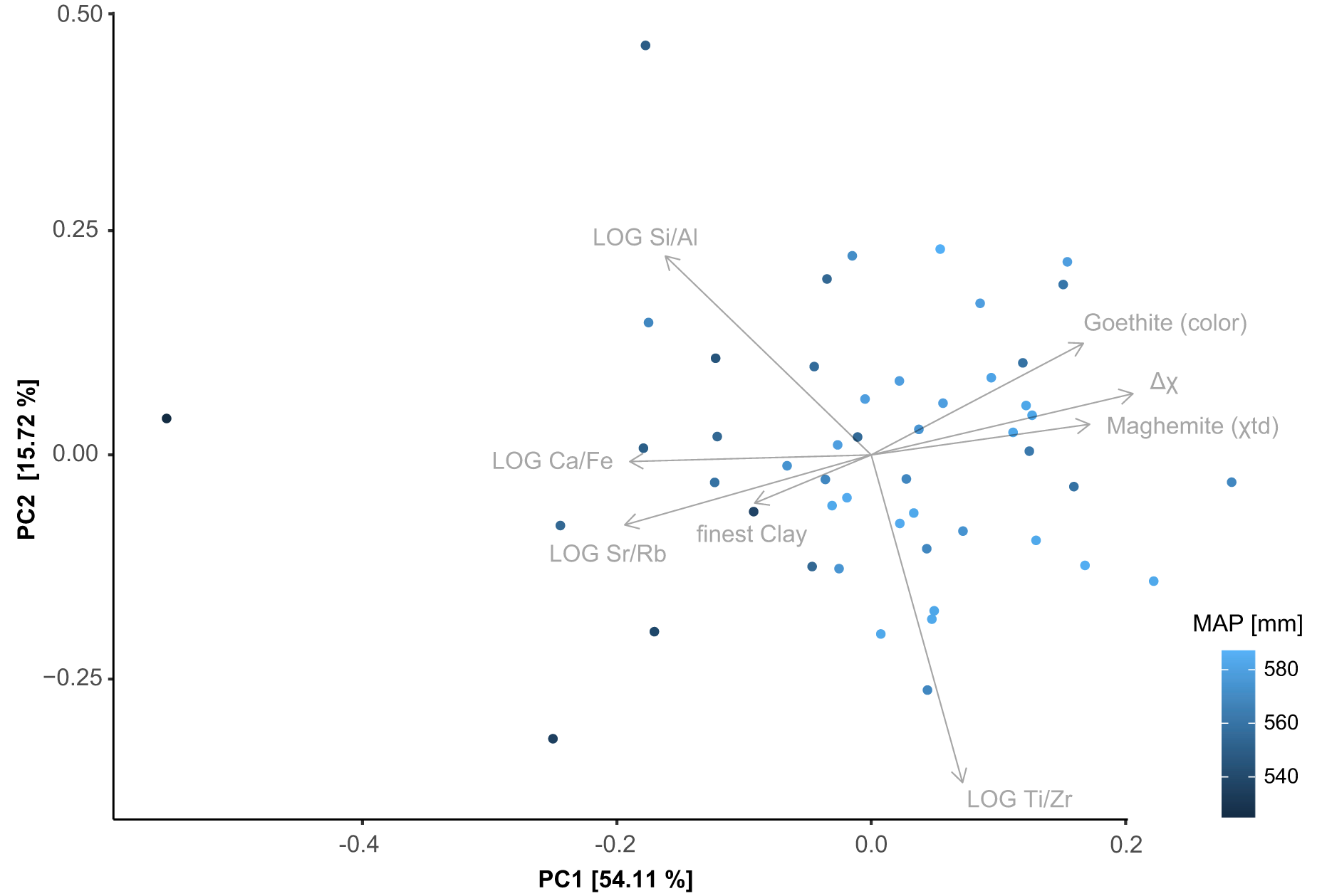
To test the possible effect of provenance shifts that may severely affect the baseline from which (chemical) alteration starts, we performed a PCA that integrates geochemical proxies frequently applied to assess provenance and grainsize shifts along with proxies that may reflect weathering (cf., Vinnepand et al., Reference Vinnepand, Fischer, Jöris, Hambach, Zeeden, Schulte and Fitzsimmons2022, and references therein; Fig. 3). For clarity, a selection of proxies was considered, and the data points are color-coded according to the MAP values at each sample locality. The first principal component (PC1) reflecting 54.1 % of the explained variance in the considered dataset spreads along the MAP gradient, however the second principal component (PC2) reflects only 15.7 % of the explained variance. Although PC2 is strongly governed by proxies that indicate provenance and sediment inhomogeneity (LOG Ti/Zr and LOG Si/Al), LOG Ti/Zr mostly drives PC2, and no relevant linear relationship can be found with grainsize fractions (clay, silt, and sand) in the overall dataset (not shown here), indicating that PC1 is predominantly governed by provenance information. In contrast, the finest clay fraction and LOG Sr/Rb (Rubidium is tightly bound to clay minerals in soils; Vinnepand et al., Reference Vinnepand, Fischer, Jöris, Hambach, Zeeden, Schulte and Fitzsimmons2022, and references therein) are far less influenced by provenance changes and align more strongly to PC1. The same applies for Δχ and the goethite content (though the goethite content appears to be more strongly influenced by provenance than Δχ), whereas the effects of provenance on maghemite are negligible and may range within the error margin of this measurement. Considering that the scores of PC1 are only moderately correlated to MAP (r 2 = 0.43), PC1 may reflect (chemical) weathering, as also indicated by LOG Ca/Fe (proxy for Ca dissolution and relative Fe enrichment), which aligns with the plane of the first principal component.
Principal component analyses (PCA) with the first principal component (PC) carrying 54.1 % of the explained variance in the dataset. While this PC is clearly dominant, it is mainly driven by all considered magnetic parameters and the LOG Ca/Fe ratio that displays carbonate dissolution, re-precitation and enrichment of Fe during weathering. Both element ratios frequently applied as provenance indicators and measure for sediment inhomogeneity (LOG Ti/Zr and LOG Si/Al) govern PC2, which is clearly not dominant (only 15.7 % of the explained variance). Based on the behavior of all integrated parameters it appears as though PC1 carries the weathering signal, whereas PC2 is generally governed by sediment provenance.

Single proxies compared to climate variables
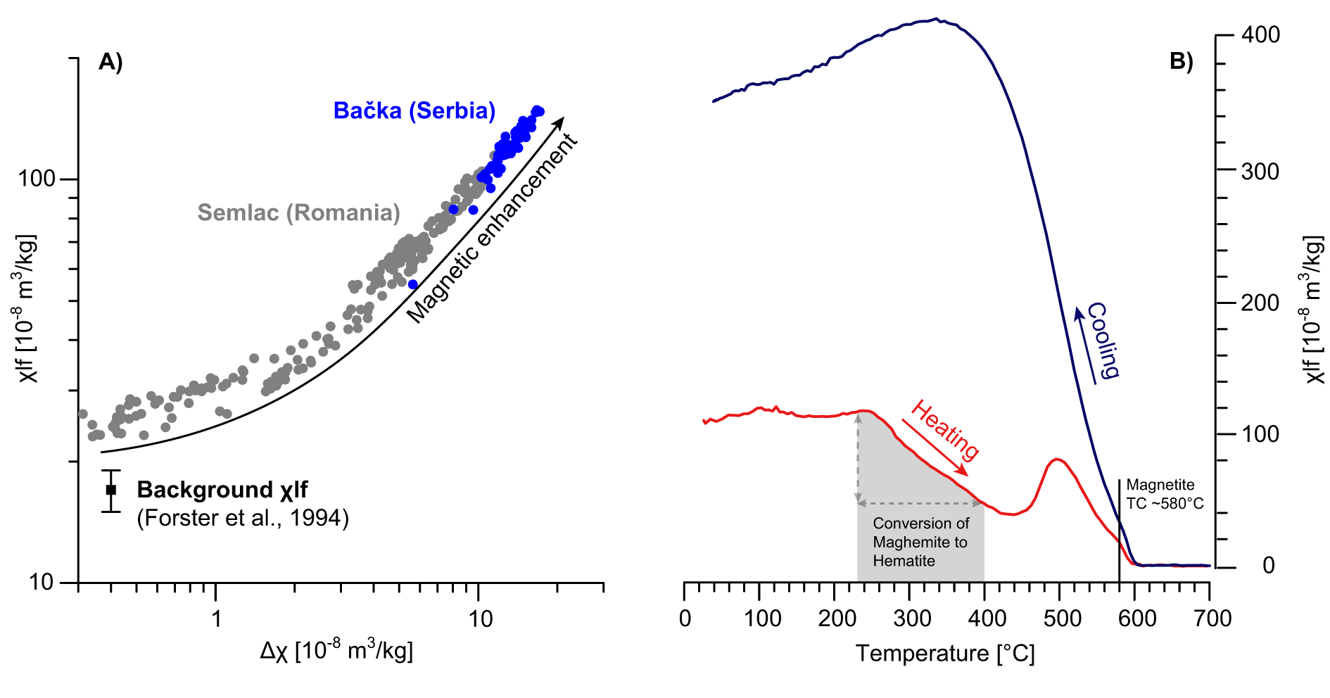
Comparing χlf to its absolute frequency dependence (Δχ) clearly shows a pedogenesis-driven magnetic enhancement in the typical range of interglacial topsoil in dry loess areas (e.g., in Semlac, Romania; Fig. 4A; Zeeden et al., Reference Zeeden, Kels, Hambach, Schulte, Protze, Eckmeier, Marković, Klasen and Lehmkuhl2016). This enhancement, combined with evidence for the presence of pedogenic maghemite and magnetite in our thermomagnetic investigations (cf., Fig. 4B), indicates ideal pre-conditions for the climate sensitivity of modern topsoils across the BLP (cf., Liu et al., Reference Liu, Roberts, Larrasoaña, Banerjee, Guyodo, Tauxe and Oldfield2012). Maghemite can be detected in thermomagnetic experiments due to the typical conversion of maghemite to hematite during heating between 230°C and 400°C leading to a drop in χlf (Gao et al., Reference Gao, Hao, Oldfield, Bloemendal, Deng, Wang and Song2019) in the absence of a prominent hump in the heating curve directly preceding this drop (cf., Zhang and Apple, Reference Zhang and Appel2023), which is the case for all our samples. Magnetite may govern parts of the remaining χlf as indicated by a drop in χlf near the Curie temperature of magnetite close to 580°C (Liu et al., Reference Liu, Roberts, Larrasoaña, Banerjee, Guyodo, Tauxe and Oldfield2012).
(A) Classic magnetic enhancement during pedogenesis as a result of the accumulation of superparamagnetic and fine-grained, single-domain particles during soil formation (Zeeden et al., Reference Zeeden, Kels, Hambach, Schulte, Protze, Eckmeier, Marković, Klasen and Lehmkuhl2016). (B) Thermomagnetic experiment indicative for maghemite on a representative sample from the BLP. Between ∼230°C and 400°C χlf drops mainly due to the conversion of pedogenetically formed maghemite to hematite during heating (Gao et al., Reference Gao, Hao, Oldfield, Bloemendal, Deng, Wang and Song2019). This can be used to calculate the maghemite content (dashed arrowed lines) by calculating the difference between χlf at 230°C and 400°C. For transparency, we provide the heating (red) and cooling (blue) χlf curves. Both may reflect mineral conversions and/or neo-formations in the experiment.

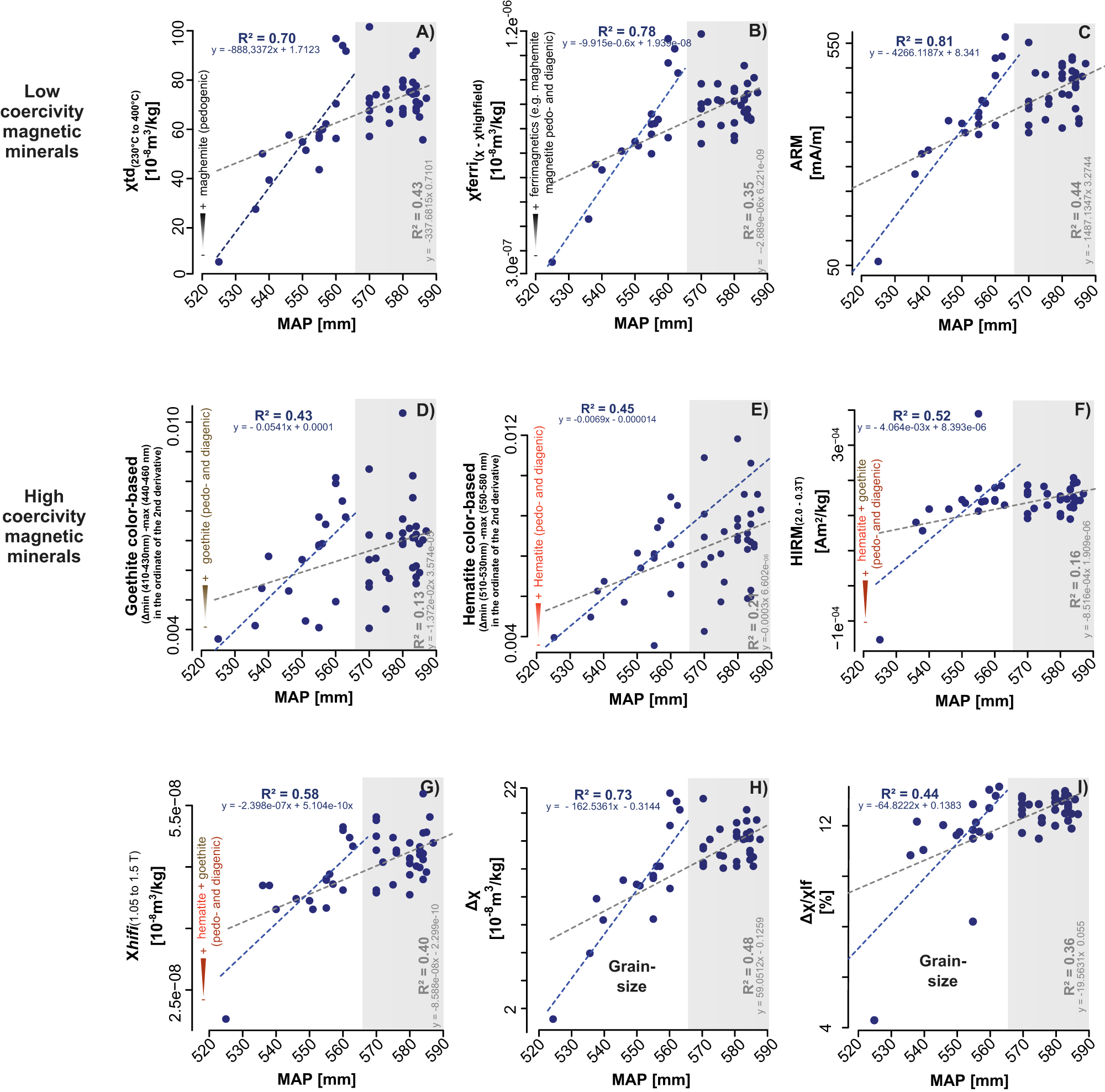
Among the investigated proxies that reflect ferrimagnetic low-coercivity magnetic minerals that typically govern the χlf, the contribution of pedogenic maghemite to χlf (χtd Fig. 5A) strongly correlates with MAP (r 2 = 0.70), considering a precipitation range between 525±1 mm/yr and 565±1 mm/yr. The relationship between the pedogenic superparamagnetic particle fraction proxied by Δχ is also very good (r 2 = 0.73; Fig. 5H). Stronger correlations with MAP are only achieved by χferri (r 2 = 0.78; Fig. 5B), which reflects magnetite and maghemite content (i.e., saturated ferrimagnetic component derived from hysteresis loops) and ARM (r 2 = 0.81), which further biases towards the finer-grained, magnetically stable magnetite and maghemite particles. The ARM shows the strongest linear relationship to MAP of all tested proxies (between MAP 525±1 mm/yr and 565±1 mm/yr).
Comparison of selected geophysical parameters with mean annual precipitation (MAP). We coarsely grouped the parameters according to their capability to display low-coercivity minerals (e.g., magnetite, maghemite), high-coercivity minerals (e.g., hematite and goethite), and grainsize-dependent parameters (some in the other groups are also mildly magnetic- and/or grainsize dependent). Almost all parameters do not strongly increase linearly with MAP considering the slope of the initial regression lines if MAP exceeds 565 mm. From this boundary onwards the selected parameters either are not as sensitive to MAP or a different (linear) best-fit line needs to be applied considering higher MAP. The best linear fit between proxies sensitive for low-coercivity magnetic minerals below MAP 565 mm (blue regression line) applies to the ARM and the isolated part of χ assigned to ferrimagnetic minerals such as pedogenic maghemite, χtd (A) and geo- and pedogenic magnetite, χferri (B). From those proxies that are sensitive for hematite and goethite (D–F), the Hard Isothermal Remanent Magnetization (F) is most promising to reflect MAP, whereas the color-reconstructed goethite and hematite contents align worse for the investigated MAP interval. Considering the entire MAP range, the strongest linear relationship can be observed between the grainsize sensitive Δχ and MAP.

All proxies that indicate for the presence of high-coercivity magnetic minerals (Fig. 5D–F) such as goethite and hematite moderately correlate with MAP—r 2 = 0.43 for the color-based goethite reconstruction (Fig. 5D); r 2 = 0.45 for the color-based hematite reconstruction (Fig. 5E); and r 2 = 0.52 for HIRM (Fig. 5F). Note that for all single-proxy correlations, if regression analyses are extended to the full range of MAP (525±1 mm/yr to 565±1 mm/yr), the r2 values are weak (between 0.13 and 0.48).
Multivariate regression analyses
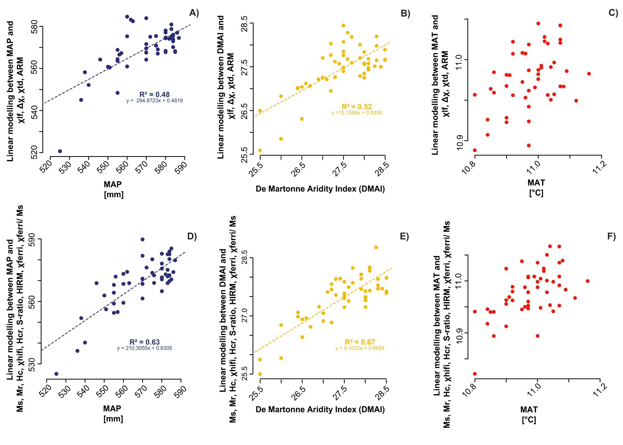
Multivariate regression analyses were carried out on the full range of MAP, on aridity index (DMAI), and on MAT using a limited number of proxies to avoid overfitting. For this we used proxies that are routinely applied in loess research and that can be determined by many laboratories (Fig. 6A–C). The same strategy was applied to hysteresis proxies, which are more sophisticated and can be determined by a limited number of laboratories (Fig. 6D–F).
(A–C) Direct comparison between MAP, DMAI, and MAT to multi-regression analyses between frequently applied magnetic proxies in loess research that can be conducted in many laboratories and climate parameters. While the linear regressions indicate a moderate relationship to climate parameters, the more sophisticated approach using hysteresis parameters (D–F) yields a stronger relationship with more than an additional 10% of the explained variance that can be aligned to these.

Starting with the linear fit between frequently applied parameters in loess research (e.g., χlf, Δχ, χtd, and ARM) with the MAP, a moderate linear relationship was established (r 2 = 0.48; Fig. 6A). This is an important finding because these relationships hold true over the entire MAP range at the BLP. Considering the single displayed proxies that are also integrated in our multi-regression analyses (Fig. 5), only Δχ, χtd, ARM, and χhifi yield comparably high r 2 values for the entire MAP range, and in the entire dataset (not displayed in Fig. 5), the bulk χ shows a moderate relationship to MAP (χlf: r 2 = 0.47, χhf: r 2 = 0.46).
In particular, the better fit for DMAI (r 2 = 0.52; Fig. 6B) compared to single-proxy investigations, indicates that multi-regression analyses that target the combined effect between MAP and MAT exhibits an enormous potential. By incorporating hysteresis parameters (Ms, Mr, Hc, χhifi, Hcr, S-ratio, HIRM, χferri, and χferri/Ms), direct linear models of MAP and DMAI consistently improve (Fig. 6D, E), with these combined parameters accounting for more than an additional 10% of the variance in MAP and DMAI. Considering MAT in both linear modeling comparisons (Fig. 6C, F), a linear relationship might be established if a wider temperature range is considered that clearly exceeds the uncertainty of 0.1 °C. Yet, MAT and the modeled MAT appear to increase simultaneously (Fig. 6C, F) to some degree, but the scatter falls mostly within the range of uncertainty.
Multivariate assessment based on principal components
Since large multivariate datasets of geophysical proxies may be more robust compared to single proxies or proxy groups, especially when it comes to proxy-specific sensitivity limitations, we combined the datasets used in our regression analyses and added the semi-quantitative hematite and goethite estimates to perform a PCA.
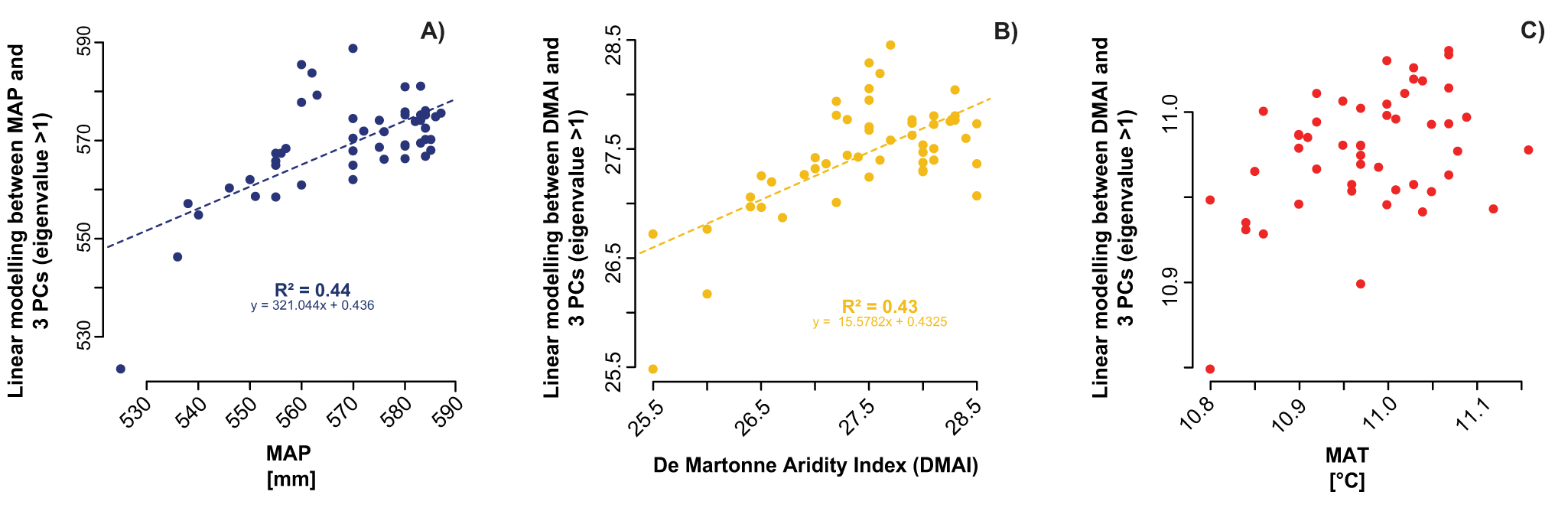
Comparing the linear fit between climate parameters and 3 principal components (PC with Eigenvalues >1) to MAP and DMAI yields promising results over the entire parameter ranges (Fig. 7). For linear modeling between MAP and 3 PCs, a r 2 of 0.44 can be ascribed to MAP and a r 2 of 0.43 can be ascribed to aridity. This is lower than for both linear models that incorporate magnetic parameters only, suggesting that the colorimetric values may apply better when considering larger MAP ranges and/or that hematite and goethite may show some provenance-related effects at the BLP.
Liner modeling between climate parameters and three principal components (all that exhibit Eigenvalues >1 extracted from a principal component analysis that we performed for all frequently applied magnetic proxies in loess research, all hysteresis parameters and the colorimetrically derived goethite and hematite contents) in comparison to the climatic parameters. For MAP and DMAI, this approach yields promising results, especially when considering the entire climatic transect range (e.g., MAP). We performed principal component analyses to achieve data-dimension reduction. This minimizes the risk for data overfitting during multi-regression analyses.

Discussion
Provenance and climate signals
Although geophysical parameters, especially magnetic proxies, have been applied frequently in loess research to study paleoenvironmental conditions with a focus on the imprint of climatic cycles (Evans and Heller, Reference Evans and Heller2003; Balsam et al., Reference Balsam, Ji and Chen2004), the influence of provenance changes on such parameters is a known feature that has been gaining increasing attention (Heller and Evans, Reference Heller and Evans1995; Grimley et al., Reference Grimley, Follmer and McKay1998; Hällberg et al., Reference Hällberg, Stevens, Almqvist, Snowball, Wiers, Költringer, Lu, Zhang and Lin2020). In the case of the BLP, we started with the premise that provenance-related effects are constrained due to its locality, for which provenance analyses indicate a relative homogenous setting (Fenn et al., Reference Fenn, Millar, Durcan, Thomas, Banak, Marković, Veres and Stevens2022). We showed that the effects of provenance may vary between single geophysical parameters, but they do not overpower the imprint of climatic parameters at the BLP—especially not considering MAP (Fig. 3).
Some investigated magnetic mineral assemblage constituents such as ferrimagnetic maghemite may be considered in certain loessic environments as predominantly of pedogenic origin (e.g., Gao et al., Reference Gao, Hao, Oldfield, Bloemendal, Deng, Wang and Song2019), but other ferrimagnetic minerals such as magnetite may also be diagenetic in origin (Liu et al., Reference Liu, Roberts, Larrasoaña, Banerjee, Guyodo, Tauxe and Oldfield2012). In the case of the BLP, four magnetic parameters show relevant correlation with MAP ranging from r 2 of 0.70 to 0.81. In increasing order, maghemite content isolated with χtd (Fig. 5A), superparamagnetic particle content isolated with Dc, total magnetite and maghemite content isolated through χferri and biased to stable single domain magnetite, and maghemite content with ARM. These results suggest strongly that provenance effects play a minor role for the ferrimagnetic mineral assemblage and provide supporting evidence for the previously observed relationship between χlf and MAP and aridity (DMAI) for the BLP by Radaković et al. (Reference Radaković, Gavrilov, Hambach, Schaetzl, Tošić, Ninkov, Vasin and Marković2019).
Interestingly, the PCA (Fig. 3) comparing the color-reconstructed goethite quantities to geochemical provenance indicators supports the interpretation that goethite content across the BLP may be governed by some limited influence of provenance differences. Such effects may explain why proxies indicative for the presence of high-coercivity magnetic minerals (Fig. 5D–F) such as colorimetrically derived goethite and hematite quantity estimates (pedo- and diagenic) only moderately correlate to MAP (goethite: r 2 = 0.43; hematite: r 2 = 0.45; Fig. 5D, E, respectively) as do HIRM (r 2 = 0.52; Fig. 5F) and χhifi (r 2 = 0.58; Fig. 5G).
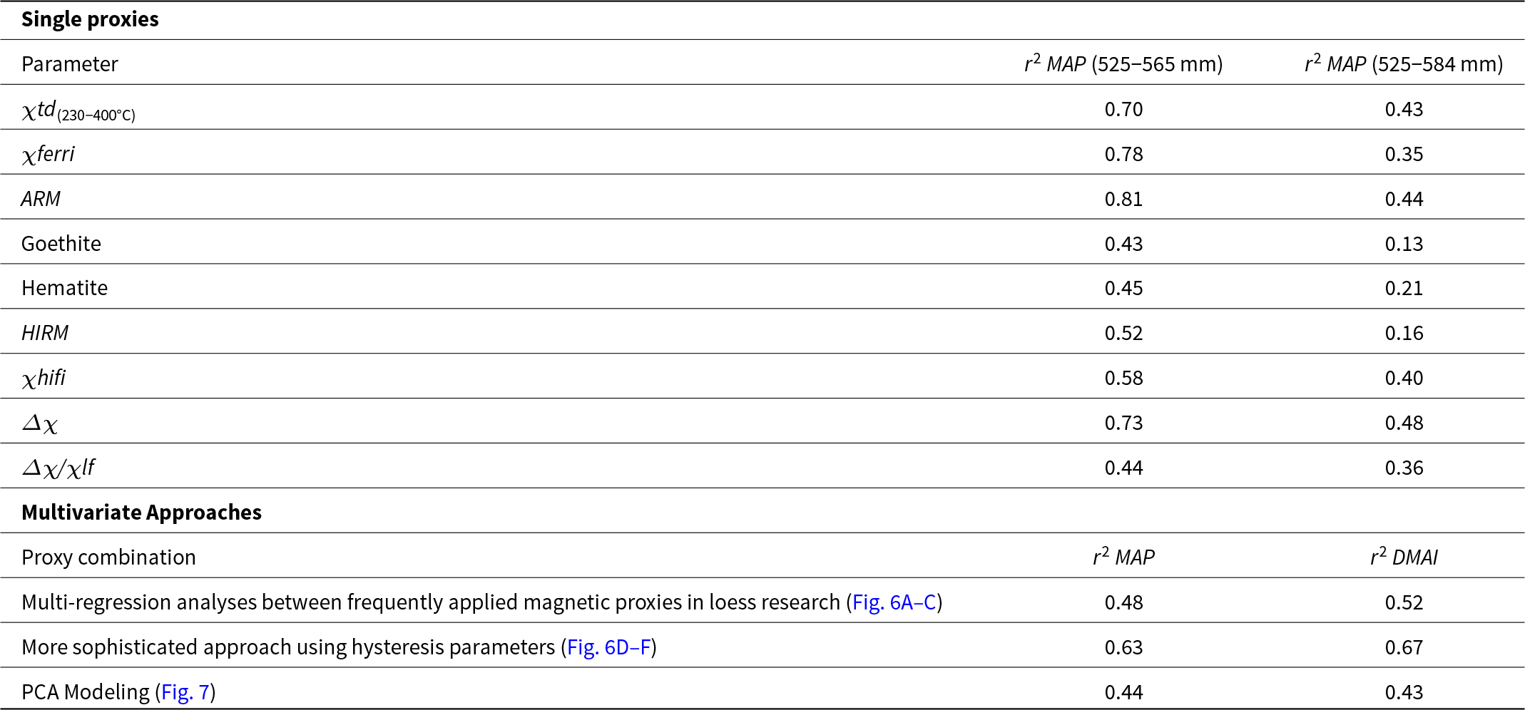
Potential of proxies considering larger climate gradients and different regressions
Considering the results of our study, it is important to note that our assessment is valid only for the investigated narrow climate gradient and needs to be extended farther back in time. Our study, therefore, does not intent to make exclusive statements about the general applicability of the integrated proxies, but instead assesses their sensitivity to the studied climatic range (table 1). Indeed, our results indicate that when a MAP threshold of ∼565 mm is exceeded, precipitation and aridity might be better approximated by other climo-functions at least in the case of all investigated rock-magnetic parameters and the color-reconstructed goethite and hematite contents. Here we are at the upper limit of precipitation amounts that usually allow for Chernozem development, and a different proxy response in different soils may be expected. However, when comparing our linear single-proxy MAP relationships (n = 50) to those established from δ13C databases for plants (Kohn, Reference Kohn2010) and more recent δ13C compilations (Rao et al., Reference Rao, Guo, Cao, Shi, Jiang and Li2017), with n = 15 and n = 78 (C3 plants uniquely) respectively in the same MAP range of 525–584 mm/yr, our results are promising even beyond the 565 mm/yr threshold. The linear MAP-δ13C relationship for this precipitation interval is weak for the Kohn et al. (Reference Kohn2010) dataset (r2 = 0.22) and the extensive Rao et al. (Reference Rao, Guo, Cao, Shi, Jiang and Li2017) dataset (r2 = 0.19) and clearly exceeded by all magnetic proxies indicative of low-coercivity minerals at the BLP (r2 ranging from 0.35-0.44, Fig. 5A-C), Χhifi (r2 = 0.40 Fig. 5G) and both measures to assess the magnetic grainsize (r2 = 0.36-0.48 (Fig. 5H, I)). In this respect, most of the magnetic parameters used are extremely promising and encourage extending the approach proposed in this study to integrate broader MAP ranges at least on a European scale to explore the potential of single proxies and proxy-combinations applied to different soils and sediment types.
Overview on the strengths of relationship between the investigated proxies, proxy combinations, and climate parameters. Here, we present r 2 values that have been obtained between single proxies and MAP below 565 mm/yr and for the entire MAP range.

Conclusions and outlook
Here we provided a comprehensive geophysical approach that compares regression analyses between single-proxy and combined multi-proxy dataset analyses and climate parameters (MAP, DMAI) across a narrow climate gradient with uncorrelated MAT and MAP trends across the Bačka loess plateau in southeastern Europe. The following main conclusions are drawn from our findings.
Cost-efficient single geophysical parameters can be effectively used to derive MAP and aridity estimates (DMAI), complementing geochemical applications, especially when MAP does not exceed ∼565 mm/yr. While this is most likely the case for stadials and interstadials even in western Central Europe (e.g., Prud’homme et al., Reference Prud’homme, Fischer, Jöris, Gromov, Vinnepand, Hatté, Vonhof, Moine, Vött and Fitzsimmons2022), other effects such as periodical waterlogging due to permafrost may limit the applicability of many geophysical parameters under colder conditions (Baumgart et al., Reference Baumgart, Hambach, Meszner and Faust2013). Testing our results in a wider climate context is encouraged.
Magnetic grainsize proxies and those sensitive to ferrimagnetic minerals (magnetite, maghemite) are highly correlated to MAP, those for high-coercivity minerals (goethite, hematite) show a weaker relationship to MAP. This demonstrates that the provenance of sediment needs to be accounted for when using most single geophysical parameters to estimate MAP.
Multivariate data analyses offer relevant advantages as they overcome limitations in the sensitivity of single proxies. Whether this is also the case for less homogenous datasets from wider regions needs to be tested.
To provide an added value and the possibility to test these relationships beyond the BLP, we published all regression functions to the single parameters, their linear multivariate combinations, and climate parameters. These can be used to calculate MAP and aridity from similar datasets and tested, if independent climate estimates are available. MAP and aridity can be reconstructed in a satisfying way from the considered geophysical properties, but MAT is more difficult to reconstruct using these tools and the uncertainty is close to the observed temperature gradient at the BLP. We emphasize that our approach needs to be tested considering different climate regimes and time slices, less homogeneous substrates and geomorphological settings, as well as fossil soils and sediments. Comparing our results to established δ13C databases that are frequently used to transfer geoscientific data into MAP estimates, shows the considerable potential of using environmental magnetic proxies for understanding soils and their formation.
Supplementary material
The supplementary material for this article can be found at https://doi.org/10.1017/qua.2025.10059.
Acknowledgments
This work was mainly funded by the Deutsche Forschungsgemeinschaft (DFG, German Research Foundation) – project number 446183251. MB is grateful for L’Oréal-UNESCO For Women in Science award and Western Balkans-Visegrad fund (#62470105). SM is grateful for the guest professorship programme of the Silesian University of Technology and Program of Cooperation with the Serbian Scientific Diaspora – Joint Research Projects – DIASPORA 2023, from the Science Fund of the Republic of Serbia, under the project LAMINATION (The Loess Plateau Margins: Towards Innovative Sustainable Conservation), Project number: 17807. Special thanks belong to Sonja Riemenschneider, Lena Wallbrecht and Kathrin Worm for their support considering sedimentological and magnetic analyses in the LIAG laboratories. We would like to thank the two anonymous reviewers as well as Nicholas Lancaster (senior editor) and Pierre Antoine (guest editor) for their constructive comments that helped to improve the manuscript.
Declaration of competing interests
The authors declare that they have no known competing financial interests or personal relationships that could have appeared to influence the work reported in this paper.
Data availability
All integrated project data will be made available in the Pangaea database after publication.
Authors statement
This paper was designed by MV and CZ and discussion took place at all stages between both authors. MB, MG, JN and SM provided the sampling material, P quantities and contributed to the discussion. Hysteresis data were generated by CL in the laboratory of FL and thermomagnetic measurements were run by KR. Colorimetric and Granulometric data were generated by MV. AD provided valuable geochemical data for provenance, substrate inhomogeneity and weathering crosschecks. Manuscript writing, editing and revision was performed by MV with input from all co-authors (CL, MB, KR, AD, MG, CR, SM, CZ, FL).


 Open access