1. Introduction

Ice-sheet flow and the deformation of the Earth in the vicinity of ice masses (‘glacial isostasy’) form an important coupled system. The coupling consists of several mechanisms. Changing ice load produces elastic Earth deformation instantaneously (on the relevant timescales), but further deformation follows from viscous upper mantle flow under the crust and lithosphere. Conversely, the changing elevation and slope of the ice-sheet bed affects ice flow through changes in elevation-dependent accumulation and surface temperatures, and also geometry-determined stress conditions. Grounding-line migration can occur, as relative sea level and sea-floor slope at the grounding line are affected by Earth deformation (Reference Lingle and ClarkLingle and Clark, 1985).

Although elaborate models exist for both ice flow and Earth deformation, the large spatial extent of ice sheets and the long timescales relevant to ice ages and paleoglacial questions strongly suggest simplifications of these models to achieve reasonable computation time. For ice-sheet flow, the full Stokes equations are usually reduced to the shallow-ice approximation or to related shallow models for ice shelves and streams (Reference HutterHutter, 1983; Reference PatersonPaterson, 1994). For the Earth deformation component of the coupled system, full spherical, layered, viscoelastic, self-gravitating models are available (Reference Le MeurLe Meur, 1996; Reference PeltierPeltier, 1998; Reference Klemann and WolfKlemann and Wolf, 1999; Reference MartinecMartinec, 2000; Reference Le Meur and HindmarshLe Meur and Hindmarsh, 2000; Reference Le Meur and HuybrechtsLe Meur and Huybrechts, 2001), but they come at large computational expense, especially for rapid load change with fine spatial scale (Reference Larsen, Motyka, Freymueller, Echelmeyer and IvinsLarsen and others, 2005). Significantly simplified Earth models are therefore currently standard for use in ice-sheet simulations (Reference Le Meur and HuybrechtsLe Meur and Huybrechts, 1996; Reference Greve, Straughan, Greve, Ehrentraut and WangGreve, 2001).

In modeling the interaction between an ice-stream model and the deforming Earth, Reference Lingle and ClarkLingle and Clark (1985) used an Earth model which is intermediate between the simplified models used in current ice-sheet simulations and full spherical models. They used as their fundamental tools the Green’s functions of two different linear Earth models. These models are reviewed below. In their original implementation the Green’s functions for these models are convolved with the load to compute vertical displacements of the Earth’s surface. They find a purely elastic displacement u ^E and a viscous displacement u given a current load and a load change history, respectively. The total displacement is then the sum u ^total = u ^E + u, that is, the two linear models are superposed. This sum gives the correct result because the combined viscoelastic Earth model is linear. In fact, for spherical Maxwell Earth models the analogous sum occurs in Love number domain (Reference PeltierPeltier, 1974, equation (51)) and also in combining Green’s functions (Reference PeltierPeltier and Andrews, 1976, equation (24)).

The partial differential equations (PDEs) behind these Green’s functions are linear, but the PDE behind the viscous half-space model has not been stated. In fact, as seems to be common in the spherical Earth deformation literature as well, the viscous model in Reference Lingle and ClarkLingle and Clark (1985) is only exploited through its tabulated Green’s functions. Displacements are computed by expensive numerical integration against load history.

The Lingle and Clark ‘two-layer’ model approximates the upper mantle as a linearly viscous half-space of viscosity η and density ρ _r, overlain by an elastic plate lithosphere of flexural rigidity D (Reference Lingle and ClarkLingle and Clark, 1985, especially fig. 3). Though it is presented in the Hankel-transformed (Reference SneddonSneddon, 1951) domain in Reference Lingle and ClarkLingle and Clark (1985), and earlier in Reference CathlesCathles (1975), it turns out that this half-space model is described by a single differential equation for vertical displacement u(x,y,t),

(1)

where g is the acceleration of gravity and σ_zz is the (ice) load force per unit area.

Here ∇⁴ is the familiar biharmonic operator which appears in equations for elastic plates (Reference SneddonSneddon, 1951), but is an operation which is defined below through the Fourier transform (Equation (6)). Note that -∇2 is a positive operator in the sense that it is self-adjoint and has non-negative spectrum (Reference Reed and SimonReed p and Simon, 1980). Thus is a real operator while would be imaginary. As we will show, reliable numerical solution of Equation (1) is not only possible but indeed very fast on a rectangular grid.

Equation (1) should be compared to the following pair of equations which describe both the bed elevation u and a notional plate elevation w for a plate which is, at all times, in equilibrium with the current load:

(2a)

(2b)

This is the standard model of an elastic plate lithosphere with relaxing asthenosphere (ELRA) widely used in ice-sheet simulation (Reference Le Meur and HuybrechtsLe Meur and Huybrechts, 1996; Reference Greve, Straughan, Greve, Ehrentraut and WangGreve, 2001; Reference HagdornHagdorn, 2003; Reference Zweck and HuybrechtsZweck and Huybrechts, 2005). Here ρ _r, D and σ_zz have the same meanings as in Equation (1), but the actual (asthenosphere) viscosity η plays no direct role. Instead, a single relaxation time τ is assumed to apply for all loads regardless of their spatial extent; τ = 3000 years is in widespread use. In other words, the bed elevation u decays toward w at a fixed rate 1/τ by Equation (2b).

In both models (1) and (2), the function u describes the top of the elastic plate lithosphere, with unloaded steady state u = 0. In these models the elastic plate lithosphere does not compress, so the top and bottom of the lithosphere are a fixed distance apart. An additional thickness u ₀ (x, y) gives detailed bed topography (e.g. mountain ranges). The super-lithosphere part of the crust described by u ₀ is assumed to be of zero strength. The true bed elevation is b = u ^E + u + u ₀ in the Lingle and Clark model and b = u + u ₀ in the standard model.

We claim that Equation (1) implements the original intent of model (2). Asthenosphere viscosity is directly incorporated, so there is no need to average over modes to give a single constant relaxation time. Time dependence is directly incorporated and this allows initialization from an uplift map. See section 4 for more on these points.

The only issue for Equation (1) is numerical implementation, and in particular the presence of the operation ∇. This is fully resolved in section 3. In section 5 we show that our implementation is fast and stable. Furthermore it computes results which agree closely with the continuum model. In fact, we demonstrate that numerical errors made in approximating coupled ice–Earth systems can be expected to be less than differences among Earth models. This is clear evidence that the correct choice of Earth model is important in ice-sheet simulations.

2. Model

As noted, Reference Lingle and ClarkLingle and Clark (1985) combine a layered spherical, self-gravitating, purely elastic Earth model with a viscous half-space overlain by an elastic plate model.

The continuum equations of the spherical elastic model are the linearized equation of conservation of momentum, the stress/strain relation of linear elasticity, and Poisson’s equation for the perturbation of the gravitational potential (Reference FarrellFarrell, 1972). Along with Reference Lingle and ClarkLingle and Clark (1985), for concreteness we adopt Farrell’s elastic Green’s functions corresponding to the ‘Gutenberg–Bullen A’ layered Earth (Reference Alterman, Jarosch and PerkerisAlterman and others, 1961). Other stratifications could be used in the same computational framework.

We incorporate this elastic Earth model entirely through its surface vertical displacement Green’s function G ^E(r), the function described by equation (37) in Reference FarrellFarrell (1972). This Green’s function is the vertical displacement caused by a 1 kg mass applied at a point on the geoid and evaluated at a distance r along the surface of the Earth from the point of application. Table A3 of Reference FarrellFarrell (1972) reports the values of G ^E(r) at particular distances, and linear interpolation of the corresponding values of rG ^E(r) gives the graph in Figure 1. We see that there is a 1/r singularity for G ^E(r), in contrast to the Green’s function for the viscoelastic half-space model used in the current paper (see Fig. 2 below). Layered and spherical elastic effects enter the Reference Lingle and ClarkLingle and Clark (1985) model, and thus the results of the current paper, through the non-trivial dependence of G ^E on the distance r. Indeed the Green’s function for vertical displacement for a purely-elastic stratified half-space is different from that shown in Figure 1, and the differences are most significant for large r (Reference FarrellFarrell, 1972).

Fig. 1.

The vertical surface displacement Green’s function GE(r) for the elastic spherical self-gravitating Earth model (Reference FarrellFarrell, 1972), shown normalized to avoid the 1/r singularity.

Fig. 2.

Green’s function G ^V(r, t) for the half-space model. From top to bottom the curves are at t = 20, 100, 200, 400, 600, 1000, 1500, 2000, 3000, 4000, 6000, 8000, 10 000, 14 000, 20 000 and 105 years.

The elastic Green’s function G ^E(r) is used as follows to compute the vertical displacement u ^E = u ^E(x, y, z) caused by elastic deformation of the spherical Earth. Suppose the load at time t is given by the function Ψ(x, y, t), with units of mass per unit area. Then

(3)

where we define and denote by R the region of the Earth’s surface containing the load. The displacement u ^E depends on time only through the changing load since elastic changes are instantaneous. In using Equation (3) we necessarily project the Earth’s geoid into a fixed plane, and this projection means our results are limited to an appropriately small region of the Earth’s surface. We implement integral (3) more-or-less directly by doing a numerical convolution (see section 3).

An important point about the model in this paper, which explains the need to include u ^E in the superposition u ^total = u ^E + u, is that the elastic plate lithosphere in the viscous half-space model deflects but does not compress. Therefore all vertical displacement u in this model is asthenosphere/ upper-mantle motion, though the elastic plate spreads the influence of any load. The just-described spherical, purely elastic Earth exhibits elastic compression, however. In practice, 12–14% of the steady-state displacement comes from u ^E while the remainder is in u from the viscous half-space model (Reference Lingle and ClarkLingle and Clark, 1985).

The viscous half-space model used by Lingle and Clark can be found from a close reading of Reference CathlesCathles (1975). In this paper, we use the particular choices of layer thickness, viscosity and flexural rigidity for the ‘two-layer’ half-space model of Lingle and Clark. Fast computation of the ‘three-layer’ model in Reference Lingle and ClarkLingle and Clark (1985) is also possible, as described in section 4 below.

To present the equation of the Cathles–Lingle–Clark viscous half-space model in its original form, we assume a load, described by its time-dependent normal force σ_zz (r,t), which is radially symmetric around a point on the Earth’s surface. Let u(r,t) be the vertical displacement of the surface. Consider its Hankel transform

(4)

where κ is the transform variable and J ₀ is the Bessel function of first kind and zeroth order (Reference SneddonSneddon, 1951). Recall that the Hankel transform of a function f (r) is the same as the Fourier transform of the corresponding function on the plane (i.e. f (x, y) where r = (x ² + y ²)^1/2). The model then says that ū solves

(5)

where is the Hankel transform of the load (Reference Lingle and ClarkLingle and Clark, 1985). The ‘two-layer’ model of Reference Lingle and ClarkLingle and Clark (1985) uses D = ET/[12(1 – v ²)] = 5.0× 10²⁴ Nm for the flexural rigidity of the lithosphere from Poisson’s ratio = 0.5, Young’s modulus E = 6.6 × 10¹⁰Nm^–2 and a thickness of T = 88 km for the elastic plate lithosphere. The density and viscosity of the fluid in the underlying half-space are assumed to be ρ _r = 3300 kgm^–3 and η = 10²¹ Pa s, respectively.

If the initial condition to Equation (5) is the condition of zero displacement and if a 1 kg load is applied at the point r = 0 and time zero, and is held there for t > 0, then ū u(, t) solving Equation (5) is the Hankel transform of Equation (1) (though that differential equation is not stated in Reference CathlesCathles (1975) or Reference Lingle and ClarkLingle and Clark (1985)). In this case we denote the displacement u(r, t) by G ^V(r, t). Equation (5) is an uncoupled set of linear first-order ODEs in time because the spatial Hankel transform has done its job and turned the underlying partial differential equation (1) into a trivially solvable system (when the load is a function of r only).

Unlike the elastic case, the Green’s function G ^V is time-dependent. A graph of G ^V for several t values is shown in Figure 2. The viscous behavior is clear, as is the role of the elastic plate lithosphere in removing any singularity at r = 0. Note that the peripheral bulge develops only at large times. Though picturing the Green’s function G ^V is useful, we will have no further need for it; G ^V plays no direct role in our numerical scheme. Furthermore we will do no numerical Hankel transforms. A method for using G ^V to compute the response to a prescribed load change history is, however, described in equations (19) and (22) in Reference Lingle and ClarkLingle and Clark (1985). We now believe that direct use of G ^V is both inefficient and unnecessary for continent-scale ice sheets.

To explain why Equations (5) and (1) are the same thing, note that the Hankel transform of is a function of the radial variable and is its Hankel transform (Reference SneddonSneddon, 1951). Thus the term in Equation (5) corresponds to ∇⁴ u. Only k > 0 is allowed in Equation (5), however, and an expression should be interpreted as . It turns out that such a first-power term may not, strictly, be interpreted as the Hankel transform of a partial differential equation. If we consider functions f (x, y) in the plane, however, and use the two-variable Fourier transform with transformed variables ξ, ζ then it is an easy calculation to show that the operation defined by

(6)

has Hankel transform is known as a pseudo-differential operator. It follows that Equation (5) is the Hankel transform of Equation (1), but in Equation (1) we have no need to assume the displacement and load are functions of r.

Equation (1) needs boundary conditions. We assume u goes to zero as (x, y) → ∞ and similarly for a sufficient number of its derivatives. We also assume that the load σ_zz (x, y, t) is always zero outside of some bounded region of interest.

Relative to the equilibrium plate with buoyant restoring force (Equation (2)), the interesting part of Equation (1) is the time-derivative term. This term accounts for viscous flow within the asthenosphere. Note that the units of the product η∂u/∂t in Equation (1) are consistent only with the half-power of the Laplacian -∇².

3. Implementation

We treat Equation (1) numerically by discretizing in time using a finite-difference method and then computing the action of the spatial derivatives |∇| and ∇⁴ using the fast Fourier transform (FFT), a famously effective implementation of the discrete Fourier transform (DFT) (Reference Briggs and HensonBriggs and Henson, 1995). The resulting method can be called a Fourier spectral collocation method (Reference TrefethenTrefethen, 2000).

We discretize in time by the trapezoid rule, analogous to the Crank–Nicolson method for the heat equation (Reference Morton and MayersMorton and Mayers, 2005), and obtain an unconditionally stable O(Δt ²) method for Equation (1). In particular, let t_n = nΔt for n = 0, 1, 2, 3, . . . and let Uⁿ (x,y) be our semi-discrete approximation of u(x, y, t_n ). Equation (1) is approximated by

(7)

Here σ_zz(x, y, t^*) = σ_zz(x, y, [(n + 1)/2]Δt if the load is known at the time t ^* = [(n + 1)=2]Δt , or σ_zz (x, y, t ^*) = (1=2)(σ_zz (x, y, t_n ) + σ_zz (x, y, tn+1)) if the load is only known at the times t_n , tn+1; both choices preserve O(Δt2) accuracy and unconditional stability.

With careful attention to the boundary condition at infinity, the time-discretized form of our PDE, Equation (7), can be well approximated by its DFT version. A reasonable way to incorporate the DFT is to assume periodicity in the spatial variables. Other boundary conditions could be applied along a boundary at sufficient distance (e.g. a clamped condition), but none of the easily implementable choices are obviously superior. For convenience we will assume a square computational region containing a smaller region of physical interest. In fact, let L be the half-length of a computational domain [-L,L] × [-L, L] which contains and may be substantially larger than the region of physical interest [-L_x , L_x ] × [-L_y , L_y ]. We apply periodic boundary conditions at x, y = ±L; we want L to act like 1 when we do this. We will verify that if L is at least twice maxfL_x , L_y } then our numerical scheme makes very small errors, and, in particular, very little error results from applying the boundary condition at finite distance.

Thus our spatial PDE problem is Equation (7) with periodic conditions on the boundary of [-L,L] × [-L, L] and the initial condition that U0(x, y) is known.

To use the DFT, we transform the problem to a standard region [–π, π] × [–π, π] Let X = πx/L, Y = πy/L Let N be an integer. Let h = 2π/N, X_j = –π + jh and Y_k = –π + kh for j, k = 1, ..., N. We use the DFT as normalized by Reference TrefethenTrefethen (2000). If f(X,Y) is some function on [–π, π] × [–π, π] with grid values f_jk = f(X_j, Y_k) then the DFT pair is

(8)

Let

(9)

be the ‘band-limited trigonometric interpolant’ of f (X, Y) (Reference TrefethenTrefethen, 2000); note the relation to the inverse DFT (8). We see that

(10)

so the Laplacian -∇² corresponds to multiplying the p, q mode by p ² + q ². Therefore |∇| and ∇⁴ are defined for functions of X, Y by, respectively, multiplication by (^p2 + q ²)¹ = ² and (^p2 + q ²)².

It follows that Equation (7) is very easy to compute if we approximate U_n (x,y) by its band-limited interpolant and compute the action of powers of the Laplacian by the multipliers above. As an algorithm, our Fourier spectral collocation method for solving PDE (1) is the sequence:

1. compute the load at time-step t_n from, for example, an ice-flow model;

2. FFT the load at

3. compute by FFT from current bed displacement values

4. let μ=π/L, k = (^p2 + q ²)¹ = ² and β = ρ ^r g + Dμ ⁴(^p2) q ²)², and compute

(11)

5. undo the transform (i.e. do inverse FFT) to obtain

6. go to (1) and do next time-step.

With standard estimates of the speed of the FFT (Reference Briggs and HensonBriggs and Henson, 1995), this method requires O ⁽N² (log2N)2) scalar operations to update the vertical displacement. We avoid the entire stage of numerically integrating viscous Green’s functions, and we have observed speed-ups of a factor of >10³ relative to implementations of such Green’s function methods. MATLAB^TM codes for an implementation of our method have been placed in the public domain.

To complete the implementation of our continuum model, recall that the total deformation in our model is the sum of u from the half-space model and u ^E from a purely-elastic spherical model. For u ^E we implement Equation (3) more-or-less directly, another O ⁽N² (log2N)2) operation per time-step if the convolution integral is approximated by a convolution sum which is implemented by the FFT. Alternatively, as described in Reference Lingle and ClarkLingle and Clark (1985), the integral can be approximated by matrix multiplication. Because purely elastic deformation is effectively instantaneous, u ^E is calculated from the current load only and the single matrix multiplication per time-step is relatively inexpensive regardless of implementation details.

4. Discussion

We can now calculate an illuminating comparison between Equation (1) and the standard model (2). Suppose that there is no load and that the vertical displacement u is a y-independent mode with wavelength : u(x, y, t) = A(t)exp(i2x/λ). In model (1) the amplitude satisfies

(12)

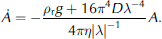
Modes have wavelength-dependent decay. By contrast, in model (2) any mode evolves by

(13)

independent of wavelength.

It is, however, clearly the case that a viscous asthenosphere will make elastic plate modes decay at different rates. Indeed, Reference Greve, Straughan, Greve, Ehrentraut and WangGreve (2001) identifies the failure of the standard model (2) to have frequency-dependent relaxation times as a deficiency of that model relative to full spherical self-gravitating models. Comparing Equations (12) and (13) we are motivated to plot the function

(14)

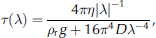
the relaxation time for a mode with wavelength . Supposing ρ ^r, g, D, η have the values given earlier for the two-layer model of Reference Lingle and ClarkLingle and Clark (1985), we have the solid curve in Figure 3. We see that the standard choice τ = 3000 years in Equation (13) represents a reasonable value and corresponds to wavelengths 300km and 3000km in Reference Klemann and WolfEquation (12), but clearly no constant relaxation time is representative of the relaxation spectrum from Equation (1).

Fig. 3.

Wavelength-dependent relaxation time (solid line) for modes evolving under Equation (1). The three-layer result with a low-viscosity channel (dashed line) is for Equation (15) with the constants given in the text. The mode-independent relaxation time τ = 3000 years (dotted line) is widely used in the standard model (2).

Following results in Reference CathlesCathles (1975), Lingle and Clark (1985) describe the modifications to Equation (5) which add a low-viscosity channel beneath the lithosphere. The modifications amount to changing Equation (1) to

(15)

where

T ^c is the thickness of the channel, ῆ is the ratio of viscosities (i.e. the viscosity of the channel divided by the viscosity of the half-space), C(k) = cosh (T_cK)and S(k) = sinhT_cK. As a minimal check on the formula for R(k), note R(k) = 1 if ῆ as must be.

The model corresponding to Equation (1) is called a ‘two-layer model’, and that corresponding to Equation (15) a ‘three-layer model’, in Reference Lingle and ClarkLingle and Clark (1985). Adopting values ῆ = 0.04 and T _c = 75 km from Lingle and Clark, we add the relaxation time for the three-layer model to Figure 3. The effect is clear: short-wavelength undulations (modes) of the lithosphere are more rapidly damped than in the two-layer model, while long-wavelength modes require deeper viscous flow and are damped at (asymptotically) the same rate as in the two-layer model. Implementation of the three-layer model is straightforward as the operator |∇| is interpreted everywhere as multiplication by (^p2+q ²)¹ / ² in the DFT variables.

It can be shown that in Equation (14) the relaxation time τ(λ) is proportional to the wavenumber k = 2π/λ for small k. That is, τ(λ) ~ 2ηk/(ρrg) as k goes to zero. The relaxation time for the three-layer model shows the same behavior, though with the viscosity being the thin channel viscosity: τ(λ) ~ 2ηchannelk/(ρrg). This behavior is identified by Reference Klemann and WolfKlemann and Wolf (1999) as a property of the most significant mode in a spherical, self-gravitating viscoelastic Earth model.

A justification for model (2a) is its computability. Indeed, approximation of the elliptic PDE (2a) is standard in all numerical paradigms (finite-difference, finite-element, spectral); the computation of (2b) is easy, of course. At least on a rectangular spatial grid, however, the time semi-discretization (7) of Equation (1) is just as computable as Equation (2a). In particular, if an ice-sheet simulation is performed on a rectangular grid using a finite-difference or finite-element method for the ice dynamics, Equation (1) can be easily computed by the Fourier spectral collocation method of the previous section. If the ice-sheet simulation is on an irregular grid or triangulation, we believe that interpolation to a regular grid, then application of our spectral collocation method, and finally re-interpolation to the irregular grid/triangulation will be an effective method. In any case, a spectral method is essentially always preferred for PDEs which have smooth solutions and coefficients and if the domain is rectangular (Reference TrefethenTrefethen, 2000; Reference Hindmarsh, Straughan, Greve, Ehrentraut and WangHindmarsh, 2001).

Note that the Fourier spectral collocation method described above can also be applied to the standard model (2) if desired.

Here is a final reason to prefer Equation (1) to (2) as a model for Earth deformation in the context of ice-sheet modeling. Suppose that the ice thickness H ₀ in a region of interest has been well measured. Suppose also that a map of uplift rate v = (∂u/∂t)| _t =₀ is also known. This is an observationally realistic supposition in many circumstances because uplift can be well constrained by global positioning system (GPS) and other measurements when bedrock is exposed (Reference Larsen, Motyka, Freymueller, Echelmeyer and IvinsLarsen and others, 2005). Alternatively a full spherical Earth model of more-or-less arbitrary sophistication and computational expense might generate a trusted current uplift map (Reference Ivins and JamesIvins and James, 2005) from an assumed load history. In either case we can then use Equation (1) to determine the initial condition for the Earth deformation part of an ice-sheet simulation without requiring further reference to the past load history. That is, we use Equation (1) to solve for u_i = uj ^{|t =} ₀,

(16)

where ρi is the density of ice. In other words, we ask for the ‘pre-bent’ position of the elastic plate in the half-space model which accounts for the current uplift rate in the presence of the current load. Solving Equation (16) numerically is essentially the same computation as one step of the numerical method in the previous section. This mechanism is, we believe, a principled replacement for the hypothesized ‘unloaded surface elevation’ sometimes used to initialize the standard model (2) (e.g. Reference Zweck and HuybrechtsZweck and Huybrechts, 2005). (Creation of such an unloaded surface elevation would appear to require an assumption of isostatic equilibrium with the load either at the present time or at the start of a model run at some past time (Reference Lingle and ClarkLingle and Clark, 1985).)

5. Results

Earth deformation only

We will verify in this section that our numerical implementation of Equation (1) reproduces the disk load case, known through a Hankel-type integral formula. This verification process reveals that a small error can be avoided if our implementation is modified slightly. The avoided error has a magnitude of a few meters uniformly in the computational domain and represents most of the effect of imposing a boundary condition, in our case a periodic condition, at finite distance.

To describe this modification and to do the verification, we note that the solution of Equation (1) on the entire plane with an ice disk load of density ρ _i, thickness H ₀ and radius R ₀ , centered at the origin, is

(17)

where β = β(k) = ρrg + Dk ⁴. A routine calculation starting from Equation (5) gives Equation (17).

We make the following simple modification to the implementation of the previous section. Consider the gridded numerical vertical displacements Uⁿ (x_j , y_k ) for Equation (1) at time t_n . Let U_nL be the average value of Uⁿ along the boundary of the computational domain [-L, L] × [-L, L]. Choose the values H ₀, R ₀ so that the volume of the disk load matches the current time t_n load volume. Let be the value from Equation (17) at t =1. Then shift the values Uⁿ (x_j , y_k ) by a constant which gives Uⁿ (x_j , y_k ) the correct ‘far-field’ value of

(18)

Note that though the volume of the equivalent disk is determined by the current load, one has freedom in choosing either its thickness or its radius. We presume that an effort can be made to approximate the aspect ratio of the actual load, but close matching is not essential; we used R0 = 1000 km for the coupled ice/Earth system results below.

We want to know that our numerical results, with the just-mentioned modification, are close to highly accurate solutions of the continuum Equation (1). The disk load case (Equation (17)) is such a solution. Let us define a particular numerical experiment. Consider a load which is a disk of ice with density ρi = 910 kgm^–3, radius 1000 km and thickness 1000 m. The center of this load will sink to a compensation depth -1000(ρi=ρr) = -276m as t !1. We seek the deflection on a square region of physical interest, centered on the disk load, of side length 4000 km, so L_x = L_y = 2000 km. Suppose that at time zero the deflection is zero everywhere, and that the load is applied at time zero. We calculate the deflection at t = 20 kyr, by our numerical method and by Equation (17).

There are three parameters of importance for our numerical implementation of the Lingle and Clark viscous half-space model:

Δx, the spatial grid size, with Δx = Δy for concreteness,

Δt, the time-step used in approximating the time derivative in (1), and

the factor by which the computational domain is larger than the physical domain.

Our verification involves showing that as the first two parameters go to their continuum limits (e.g. Δx → 0 and Δt → 0) we rapidly approach the exact solution (17). Brief experimentation with large computational domains also reveals that, as long as the above-described modification is applied, it suffices to use a computational domain which is a factor of two larger than the region of interest.

If we fix Δt = 500 years and then consider the effect of spatial grid refinement, we see that relatively coarse grids give acceptably small errors. Maximum and average error, over all gridpoints in the region of physical interest, are shown in Figure 4. The coarsest grid has Δx = 500 km and this value is halved five times. Figure 4 shows that the average bed elevation error is <20cm for Δx = 15 km, or roughly 0.07% of the compensation depth.

Fig. 4.

Maximum and average bed elevation error made by our numerical scheme for Equation (1), relative to the exact solution (17) of the disk load problem. Here Δt = 500 years.

On this finest 15 km grid, a 267 × 267 grid, and using a MATLAB^TM implementation, a 20 kyr model year run took only about 20 s. Compared to the computational expense of thermocoupled ice-sheet simulations, this Earth model is effectively free.

In fact Δt = 500 years is not too long a time-step. We compare the effects of spatial grid refinement to reduction of time-step Δt on the error in Figure 5. We see there is no benefit of Δt < 500 years. This is good, not surprising, news for ice-sheet simulation because of the relative timescales of ice vs asthenosphere flow. Relaxation times in the three-layer model are somewhat shorter, but time-steps of length Δt = 100 years certainly suffice in that case.

Fig. 5.

Average bed elevation error as in Figure 4 but with Δt varying, and for several values of Δx. Spatial grid refinement is much more important to reducing error than is temporal refinement (decreasing Δt ).

Coupled ice flow and Earth deformation

Earth deformation in the context of ice-sheet modeling is our actual interest, so next we seek to verify results for coupled ice-flow/Earth-deformation systems. The simplest representative ice-sheet model is the isothermal shallow model with Glen rheology (Reference Huybrechts and PayneHuybrechts and others, 1996). Let h(x, y, t) be the surface elevation of the ice and H(x, y, t) be the ice thickness. If b(x, y, t) is the ice-sheet bed elevation then

h = b + H. The frozen-base isothermal ice-sheet equation is the non-linear diffusion (partial differential) equation

(19)

where M(x, y, t) is the ice equivalent accumulation rate, n is the Glen exponent for ice flow and Γ is a constant. We use n = 3, Γ = 2(ρig)nA0=(n + 2) and A ₀ = 10^-16 Pa^–3 a^–1.

As we now show, exact similarity solutions to Equation (19) which incorporate pointwise isostasy (Reference HalfarHalfar, 1983; Reference NyeNye, 2000; Reference Bueler, Lingle, Kallen-Brown, Covey and BowmanBueler and others, 2005) provide a nice tool to examine coupling to the Earth model and illuminate the differences among Earth models. By ‘pointwise isostasy’ we mean the rule which specifies

(20)

where f is a fixed fraction of the ice thickness; we use f = ρi=ρr here. Since h = b + H, if Equation (20) applies then h = (1 - f )H.

We compare numerical results for three coupled ice-sheet-flow–Earth-deformation models:

POINTWISE: Equations (19) and (20),

STANDARD: Equations (2), (19) and b = u,

Lingle and Clark (L&C):

Equations (1), (3), (19) and b = u ^E + u.

There is no detailed bed topography so u ₀(x, y) = 0.

Figure 6 shows a profile of the coupled simulation for these three models at 60 kyr. The most obvious difference is the deeper descent of the center of the sheet in the L&C model. This comes from the inclusion of spherical elastic compression, which is missing in the other two models.

Fig. 6.

Ice sheet on deforming bed, at time 60 kyr, from three Earth models POINTWISE, STANDARD and L&C. View of gridded numerical values (on a 192 × 192 grid) along the positive x axis of the grid. Note differences in descent depth at center and differences at the margin of the ice sheet.

The result shown in Figure 6 came from starting with H = 0 and b = 0 at t = 0 and using an accumulation history corresponding to the = 5 similarity solution in Reference Bueler, Lingle, Kallen-Brown, Covey and BowmanBueler and others (2005). The accumulation M comes from Equation (10) in Reference Bueler, Lingle, Kallen-Brown, Covey and BowmanBueler and others (2005), using n = 3, f = 910=3300, α = -1, β = 2, H ₀ = 3600 m, R ₀ = 750 km and Γ = 9.0177 × 10^-13 m^–3 s^–1. Note t ₀ =40 034 years is the characteristic timescale for this similarity solution (Reference Bueler, Lingle, Kallen-Brown, Covey and BowmanBueler and others, 2005, equation (9); cf. Reference NyeNye, 2000)). At time t = t ₀ the accumulation is turned off, so for t > t ₀ the exact solution to the POINTWISE model is a version of the

Reference HalfarHalfar (1983) accumulation-free similarity solution incorporating pointwise isostasy. Thus the accumulation history is from a similarity solution to Equations (19) which grows from zero ice at t = 0 to maximum ice thickness of 3600 m at t ₀ =40 034 years. It spreads out from then on, with no change in volume, and at all times the Earth is in equilibrium with the load according to Equation (20).

The importance of such a similarity solution is that it forms an exact continuum solution to the POINTWISE model. Therefore we can answer with some precision the question ‘how do differences resulting from coupling to various Earth deformation models compare to the numerical errors which occur in ice-sheet modeling?’ If numerical ice-sheet errors demonstrably exceed the Earth model differences then we should be skeptical of any expenditure of effort in the Earth-modeling direction. On the other hand, if the differences among Earth models are significant, when coupled with a given ice-flow simulation, one would want to report these differences relative to the actual magnitude of numerical ice-modeling errors.

The differences among models can be expressed in terms of both bed-elevation and ice-thickness maps. In Figure 7 we show the maximum and average pairwise absolute bed elevation differences jb _POINTWISE - b _STANDARD ^j, etc. POINTWISE vs STANDARD shows somewhat smaller differences while the differences between POINTWISE and L&C are largest.

Fig. 7.

Maximum and average bed elevation differences in pairwise comparison of coupled (ice)/(earth) models.

Now, are such differences significant to numerical simulations of ice flow? The answer shown in Figure 8 is yes. Ice-sheet flow simulations on grids inevitably make large thickness errors near the margin (Reference Bueler, Lingle, Kallen-Brown, Covey and BowmanBueler and others, 2005; Reference Saito, Abe-Ouchi and BlatterSaito and others, 2007). These errors decay only slowly under grid refinement. Figure 8, however, shows that when we compare the average numerical ice-thickness errors made in the POINTWISE model with pairwise average thickness differences among the three coupled ice-flow/Earth-deformation models, we see that differences between the coupled models exceed the numerical error when the grid is even modestly refined. This comparison shows the differences among coupled ice/Earth models are numerically significant in a sense which is analogous to a claim of ‘statistically significant differences’ in a more traditional experimental context.

Fig. 8.

Average ice-thickness differences (pairwise comparison) between coupled ice/Earth models compared to average numerical errors for the pointwise isostasy case. Display format for differences is the same as in Figure 7. This comparison demonstrates numerical significance of our (numerical) result that the models produce different coupled outcomes.

6. Conclusions

The standard ELRA model (2) is regarded by many in the ice-sheet modeling community as sufficient because it gives results reasonably close to those from full spherical models (Reference Greve, Straughan, Greve, Ehrentraut and WangGreve, 2001).We do not dispute this claim, though whether any model is close enough clearly depends on modeling goals and needs. (Such questions are not addressed in this methodological paper anyway.) Our model is promising, however, because it is just as computationally inexpensive as the standard model while it also incorporates at least two important features of more complete Earth models, namely (i) mode-dependent relaxation times and (ii) elastic deformation of the spherical, layered, self-gravitating Earth.

We expect that our model will also provide better predictions of uplift rates because of the direct inclusion of the asthenospheric viscous diffusion process. This should be especially true in the vicinity of ice-sheet margins and ice-stream grounding lines. Also, it is easier in our model to provide suitable initial conditions for coupled ice-sheet and Earth deformation models without assuming unrealistic unloaded basal topographies. One can use observed uplift rates, if available, to initialize such models.

The linearity of the underlying Maxwell Earth model justifies superposing upon the result u of Equation (1) a purely elastic displacement u ^E using tabulated values of Green’s functions from Reference FarrellFarrell (1972). Separate computation of purely-elastic and viscous surface displacements then opens the possibility of adjusting the constants in our model to fit results coming from observed uplift rates and full spherical viscoelastic models. The sum u _total = u ^E + u could be replaced by some other linear combination u ^total = αu ^E + βu if that was warranted by geophysical observations or by comparison to full spherical models.

Indeed, speaking abstractly, the possibility also exists to take spherical effects into account within the same class of computationally inexpensive two-spatial-variable PDEs like Equation (1). Equation (1) would be computable at nearly the same speed if it were replaced by a non-constant coefficient version (Reference TrefethenTrefethen, 2000). We do not yet know if a set of non-constant coefficients (i.e. non-constant η, ρ _r, D in Equation (1)) exist which correctly account for spherical geometry. We do know, however, that for a Maxwell Earth (Reference PeltierPeltier, 1974; Reference PeltierPeltier and Andrews, 1976) the mathematical mapping from present surface load and displacement to present uplift is linear. Combined with the causality and regularity of the model, the linearity of this mapping makes it mathematically inevitable that a two-spatial-dimension (map-plane), non-constant coefficient linear equation for the vertical displacement of the Earth’s surface must exist. That equation may well involve additional pseudo-differential operators not present in Equation (1) or (15), however.