






1. Introduction
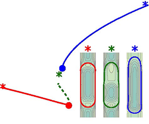
The flow of an elongated gas bubble in a cylindrical vertical tube is of interest in many industrial applications, such as flows in porous media, enhanced oil recovery (Kovscek & Radke Reference Kovscek and Radke1994) and coating processes, e.g. Yu, Khodaparast & Stone (Reference Yu, Khodaparast and Stone2018a). The dynamics of the bubble is determined by the interaction of gravitational, interfacial, viscous and inertial parametric forces. One flow regime is that of negligible inertia and dominant capillary forces. In this case, the elongated bubble traps a thin film of liquid against the channel wall, and the front and rear menisci are separated by a region of uniform film thickness (Bretherton Reference Bretherton1961; Bashforth et al. Reference Bashforth, Fraser, Hutchison and Nedderman1963; Yu et al. Reference Yu, Zhu, Shim, Eggers and Stone2018b; Magnini et al. Reference Magnini, Khodaparast, Matar, Stone and Thome2019). A recent study by Yu et al. (Reference Yu, Magnini, Zhu, Shim and Stone2021) also focused on this regime and showed the existence of two different flow configurations for the same values of the control parameters when the Bond number exceeded a critical value within a range of the imposed downward external capillary number. These results were unexpected in an operating regime where the inertial forces of the fluid, responsible for an important part of the nonlinear terms of the equations governing the bubble dynamics, are negligible. Another interesting result found by Yu et al. (Reference Yu, Magnini, Zhu, Shim and Stone2021) is the loss of bubble symmetry in the parameter range within which there is a multiplicity of solutions. Numerous experimental studies had already reported this phenomenon but in the regime of large inertial forces (Figueroa-Espinoza & Fabre Reference Figueroa-Espinoza and Fabre2011; Fabre & Figueroa-Espinoza Reference Fabre and Figueroa-Espinoza2014; Fershtman et al. Reference Fershtman, Babin, Barnea and Shemer2017). In these cases, there is a critical liquid velocity beyond which the bubble shape loses axisymmetry. The viscously dominated flow limit is the focus of this paper.
To the best of our knowledge, the study by Lu & Prosperetti (Reference Lu and Prosperetti2006), who performed a linear stability analysis of a buoyant Taylor bubble moving in a downward flowing liquid, using potential flow theory and with negligible surface tension, represents the first attempt in the literature to understand via linear theory the mechanism behind the transition of the bubble shape from symmetric to asymmetric profiles in the inertial regime. In particular, and in agreement with experimental observations, they found that a bubble subjected to irrotational flow perturbations becomes unstable beyond a negative critical (downward) liquid velocity. More recently, Abubakar & Matar (Reference Abubakar and Matar2022) studied a Taylor bubble translating at constant speed in stagnant and flowing liquids and performed a global stability analysis using a domain perturbation method (Carvalho & Scriven Reference Carvalho and Scriven1999) for a wide range of control parameters. They found numerous examples in which the bubble loses stability under a non-axisymmetric perturbation with azimuthal wavenumber  $|m|=1$. However, they did not explore the parametric region analysed by Yu et al. (Reference Yu, Magnini, Zhu, Shim and Stone2021), who characterised the bubble shape and motion for Bond number of order unity with negligible inertia, nor did they report the existence of a multiplicity of axisymmetric steady solutions.
In this work we implement a variant of the numerical technique developed by Herrada & Montanero (Reference Herrada and Montanero2016), which is based on the use of analytical Jacobians and non-singular mappings for flows with a free interface. This approach has been used for the global linear stability studies of different multiphase flows, such as electrosprays (Ponce-Torres et al. Reference Ponce-Torres, Rebollo-Munõz, Herrada, Ganãn-Calvo and Montanero2018) and flows in channels with hyperelastic walls (Herrada et al. Reference Herrada, Blanco-Trejo, Eggers and Stewart2022). The method developed here allows the study of bubbles and droplets flowing in tubes because it includes the complete modelling of the interior phase. However, in this work it will be used only to study elongated bubbles in tubes for the same parameters as those reported by Yu et al. (Reference Yu, Magnini, Zhu, Shim and Stone2021) in order to explain the existence of a multiplicity of axisymmetric solutions and the loss of symmetry of these solutions observed both experimentally and numerically.
The rest of the paper is organised as follows. In § 2 we provide details of the governing equations and the numerical techniques used to carry out the computations of the steady axisymmetric flows and the stability analysis. In § 3, a discussion of the base state results is given and the linear stability analysis is presented. Finally, concluding remarks are provided in § 4.
2. Model formulation
We consider the configuration sketched in figure 1, where an elongated bubble of a gas of density  $\rho _g$, viscosity $\mu _g$ and volume $V$ rises in a cylindrical vertical capillary of radius $R$ containing a liquid of density $\rho _l$ and viscosity $\mu _l$. To model the movement of the bubble under the combined action of gravitational acceleration $g$ and an imposed flow rate through the tube $Q$, the system is solved in a frame moving with the bubble where a non-inertial cylindrical coordinate system ( $r$,
$r$,  $\theta$, $z$) aligned with the gravity vector and anchored to the bubble is selected. This system is, in turn, linked to an inertial Cartesian coordinate system ( $X$,
$X$,  $Y$,
$Y$,  $Z$) anchored to the tube walls and also aligned with the gravity field and the non-inertial system. To model the apparent forces in the momentum equations in this non-inertial coordinate system, we have to include all of the accelerations of the system. In our case, since both coordinate systems are aligned, we will only have to consider the axial acceleration $\boldsymbol {a}=({{\rm d} U}/{{\rm d} t}) \boldsymbol {e}_{Z}$ of the reference frame, where $U(t)$ is the axial velocity of the top point of the liquid–gas interface (green arrow in figure 1) and $U_l=Q/({\rm \pi} R^2)$ is the mean velocity of the liquid flowing through the tube (both velocities measured in the inertial Cartesian coordinate system). Figure 1 also indicates the computational domain used in the simulations (a cylinder of radius $R$ and length $H$) and the boundary conditions applied at the outer boundaries of this domain.
Sketch of the flow geometry considered in this study: a bubble rising in a tube with an applied axial flow.

2.1. Governing equations
The conservation of mass and a balance of linear momentum in the liquid ( $i=l$) and gas ( $i=g$) subdomains is given by
 $$\begin{gather} \boldsymbol{\nabla}\boldsymbol{\cdot}\boldsymbol{v}_i = 0,\quad (i=l,g), \end{gather}$$
 $$\begin{gather}\rho_i\left(\frac{\partial \boldsymbol{v}_i}{\partial t} + \left(\boldsymbol{v}_i\boldsymbol{\cdot}\boldsymbol{\nabla}\right)\boldsymbol{v}_i\right) = \boldsymbol{\nabla}\boldsymbol{\cdot}\boldsymbol{\sigma}_{i},\quad (i=l,g), \end{gather}$$
where  $\boldsymbol {v}_i=w_i \boldsymbol {e}_z+u_i \boldsymbol {e}_r+v_i \boldsymbol {e}_\theta$ is the velocity field and $\boldsymbol {\sigma }_i$ is the stress tensor of material $i$ (
$i$ ( $i=g,l$). We consider in both regions the incompressible flow of a Newtonian fluid, where the stress tensor takes the form
 \begin{equation} \boldsymbol{\sigma}_{i}={-}p_i \boldsymbol{I}+ \mu_i\left(\boldsymbol{\nabla}\boldsymbol{v}_i+ \boldsymbol{\nabla}\boldsymbol{v}_i^{\rm T}\right),\quad (i=l,g) \end{equation}
where  $p_i$
$p_i$  $(i=l,g)$ is the reduced pressure, $p_i=p_i^*+\rho _i g z+\rho _i ({{\rm d} U}/{{\rm d} t}) z$, $p^*$ is the static pressure and the other two terms arise from the gravitational potential and the potential associated with the linear acceleration of the reference frame, respectively.
At the top boundary,  $z= H/3$, (see figure 1) we assume a parabolic axial velocity profile
 \begin{equation} w_{l}={-}U(t)+2U_l[1-(r/R)^2],\quad u_{l}=0,\quad v_{l}=0.\end{equation}
At the bottom,  $z=-2H/3$, the static pressure is set to zero
 \begin{equation} p_l^*=0. \end{equation}
 At the wall,  $r=R$, no-slip boundary conditions are applied
 \begin{equation} w_l={-}U(t),\quad u_l=0,\quad v_l=0. \end{equation}
 Across the gas–liquid interface (see magenta line in figure 1), parametrised in terms of a meridional arc length  $s$ (
$s$ ( $0\leq s\leq 1$) and the azimuthal angle $\theta$, $r_I=F(s,\theta,t)$ and $z_{I}=G(s,\theta,t)$, we impose that the velocity field must be continuous, i.e.
 \begin{equation} w_l=w_g,\quad u_l=u_g,\quad v_l=v_g,\end{equation}
and impose a balance of normal and tangential stresses between the liquid and the gas in the form
 $$\begin{gather} \boldsymbol{n}\boldsymbol{\cdot}({\boldsymbol \sigma}_{l}-\boldsymbol{\sigma}_{g})\boldsymbol{\cdot} \boldsymbol{n}= \gamma \kappa +(\rho_l-\rho_g)\left(g +\frac{{\rm d} U}{{\rm d}t}\right) z_I, \end{gather}$$
 $$\begin{gather}\boldsymbol{t}_1\boldsymbol{\cdot}({\boldsymbol \sigma}_{l}-\boldsymbol{\sigma}_{g})\boldsymbol{\cdot} \boldsymbol{n}=0,\quad \boldsymbol{t}_2\boldsymbol{\cdot}({\boldsymbol \sigma}_{l}-\boldsymbol{\sigma}_{g})\boldsymbol{\cdot} \boldsymbol{n}=0, \end{gather}$$
where
 \begin{align} \boldsymbol{n} = \frac{G_s \boldsymbol{e}_r-F_s\boldsymbol{e}_z+ (F_s H_\theta-F_\theta G_\theta)/F\boldsymbol{e}_\theta }{[G_s^2+F_s^2+ ((F_s G_\theta-F_\theta G_\theta)/F)^2]^{1/2}},\quad \boldsymbol{t}_1 = \frac{G_s\boldsymbol{e}_z+ F_s\boldsymbol{e}_r }{(F_s^2+G_s^2)^{1/2}},\quad \boldsymbol{t}_2= \boldsymbol{n}\times \boldsymbol{t}_1, \end{align}
are normal ( $\boldsymbol {n}$) and tangential vectors ( $\boldsymbol {t}$) to the surface, the subscripts $s$ and $\theta$ represent derivatives with respect to $s$ and $\theta$, respectively, $\kappa =\boldsymbol {\nabla }\boldsymbol {\cdot }\boldsymbol {n}$ is twice the mean curvature and $\gamma$ is the surface tension. In addition, the kinematic boundary condition on the interface is written
 \begin{equation} \left(u_l-\frac{\partial F}{\partial t}\right)\frac{\partial G}{\partial s}- \left(w_l-\frac{\partial G}{\partial t}\right)\frac{\partial F}{\partial s}+ \frac{v_l}{F}\left(\frac{\partial F}{\partial s}\frac{\partial G}{\partial \theta}- \frac{\partial F}{\partial \theta}\frac{\partial G}{\partial s}\right)=0.\end{equation}
 To ensure a uniform distribution of points along the arc length  $s$, the following equation is applied:
 \begin{equation} \frac{\partial F}{\partial s}\frac{\partial^2 F}{\partial s^2}+ \frac{\partial G}{\partial s}\frac{\partial^2 G}{\partial s^2}=0. \end{equation}
At the axis,  $r=0$, regularity conditions are considered.
Finally, to close the problem we need an additional condition for the bubble velocity  $U(t)$, which is unknown if the flow rate $Q$ is considered specified. This is achieved by imposing that a particular point of the interface has a zero axial velocity in the non-inertial reference frame. Therefore, we choose that the top point of the interface crossing the axis verifies
 \begin{equation} w_l=0,\quad z_I=G=0, \quad r_I=F=0, \quad at \quad s=1. \end{equation}
For unsteady simulations, the kinematic equation (2.1k) and the continuity equations (2.1a) guarantee that the volume of the bubble remains constant during the simulation. However, for steady axisymmetric simulations, to fix the volume of the bubble, the following additional equation must be imposed:
 \begin{equation} V=\int_0^1 {\rm \pi}F^2\frac{\partial G}{\partial s} {\rm d} s. \end{equation}
More details on the discretisation of the domains and the additional equations needed to solve the problem are given in Appendix A.
2.2. Axisymmetric steady solutions
Steady-state solutions of the nonlinear equations (2.1) with all variables independent of time and  $\theta$ are obtained by solving all equations simultaneously (a so-called monolithic scheme) using a Newton technique. We denote the steady axisymmetric solution of the system with the subscript $b$. The steady bubble profile $h_b(s)$, is defined as
 \begin{equation} h_b(s)=R-F_{b}(s),\quad 0\leq s\leq1. \end{equation}
 As described in Yu et al. (Reference Yu, Magnini, Zhu, Shim and Stone2021), for long bubbles  $h_b$ is characterised by three distinct regions: I the bubble ‘nose’ $h_b\neq cte$; II, uniform film region $h_b(s)=cte=b$; and III, the bubble ‘tail’ $h_b\neq cte$ (see figure 2). We trace the steady solutions as a function of the model parameters and quantify them using the steady bubble length, $L_b$, defined as
 \begin{equation} L_b=\int_0 ^1 \sqrt{\left(\frac{\partial G_b}{\partial s}\right)^2+ \left(\frac{\partial F_b}{\partial s}\right)^2} {\rm d} s. \end{equation}
Steady bubble profile  $\hat {h}_b$ as a function of the axial coordinate $\hat {z}$ for $Bo=0$, $\hat {V}=3.3$ and two external capillary numbers showing three different regions: ‘nose’, ‘uniform film region’ and the ‘tail’. Theoretical predictions for $\hat {b}$ given by Bretherton (Reference Bretherton1961) and extended by Aussillous & Quéré (Reference Aussillous and Quéré2000) are also depicted for comparison.

2.3. Nonlinear axisymmetric dynamical simulations
The numerical method can be extended to compute unsteady solutions. Temporal derivatives are discretised using second-order backward differences and at each time step the resulting system of (nonlinear algebraic) equations is solved using the Newton technique (as in § 2.2). The simulations use the same mesh as the stationary simulations with a fixed time step to calculate the time transition between the two stable axisymmetric stationary solutions. To characterise these unsteady solutions we will use the bubble profile defined as
 \begin{equation} h(s,t)=R-F(s,t),\quad 0\leq s\leq1, \end{equation}
and the bubble length,  $L(t)$, defined as
 \begin{equation} L(t)=\int_0 ^1 \sqrt{\left(\frac{\partial G}{\partial s}\right)^2+ \left(\frac{\partial F}{\partial s}\right)^2} {\rm d} s. \end{equation}
2.4. Small amplitude three-dimensional perturbations
To test the stability of a given steady axisymmetric state we calculate the linear global modes by assuming the temporal and azimuthal dependencies
 \begin{equation} \varPsi(r,\theta, z;t)=\varPsi_b(r,z)+\epsilon \delta \varPsi(r,z)\exp({-{\rm i}\omega t+{\rm i}m\theta})\quad (\epsilon\ll 1), \end{equation}
where  $\varPsi (r,\theta,z;t)$ represents any dependent variable while $\varPsi _b( r,z)$ and $\delta \varPsi (r, z)$ denote the base (steady) solution and the spatial dependence of the eigenmode for that variable, respectively, while $\omega =\omega _r+{\rm i}\omega _i$ is the frequency (an eigenvalue) and $m$ is the azimuthal wavenumber. For a given $m$, both the eigenfrequencies and the corresponding eigenmodes are calculated as a function of the governing parameters. The dominant eigenmode is that with the largest growth factor $\omega _i$, so that if it is positive, the base flow is asymptotically unstable.
The numerical procedure used to solve the steady problem can be easily adapted to solve the eigenvalue problem that determines the linear global modes of the system. In this case, the temporal and azimuthal derivatives are computed assuming the dependence (2.6). The spatial dependence of the linear perturbation  $\delta \varPsi ^{(q)}$ is the solution to the generalised eigenvalue problem $\mathcal {J}^{(p,q)}_b\delta \varPsi ^{(q)}={\rm i}\omega \mathcal {Q}^{(p)}_b \delta \varPsi ^{(q)}$, where $\mathcal {J}^{(p,q)}_b$ is the Jacobian of the system evaluated with the basic solution $\varPsi _b^{(q)}$ and $\mathcal {Q}^{(p,q)}_b$ accounts for the temporal dependence of the problem. This generalised eigenvalue problem is solved using the Matlab eigs function.
2.5. Control parameters
To non-dimensionalise the system we use the tube radius  $R$, the surface tension $\gamma$ and the liquid viscosity $\mu _l$. The resulting problem is governed by six dimensionless parameters
 \begin{equation} Re=\frac{\rho_l\gamma R}{\mu_l^2},\quad Bo=\frac{\rho_l G R^2}{\gamma},\quad Ca_l= \frac{\mu_l U_l}{\gamma},\quad \rho=\frac{\rho_g}{\rho_l},\quad \mu=\frac{\mu_g}{\mu_l},\quad \hat{V}=\frac{V}{4/3{\rm \pi} R^3}.\end{equation}
Here,  $Re$ is a Reynolds number based on the natural velocity $\gamma /\mu _l$, $Bo$ is the Bond number, $Ca_l$ is the external capillary number based on the mean liquid speed, $\hat {V}$ is the dimensionless bubble volume and $\rho$ and $\mu$ are the density and viscosity ratios, respectively. In this work we will neglect the inertia of the fluids by letting $Re\to 0$ and we fix density and viscosity ratios, $\rho =0.000949$ and $\mu = 0.000018$, which correspond to the experimental values of air bubbles in glycerol used by Yu et al. (Reference Yu, Magnini, Zhu, Shim and Stone2021). In the simulations, the length of the computational domain will be kept fixed, $\hat {H}={H}/{R}=15$. The main dimensionless equations are given in Appendix B.
3. Results
In this section we predict the bubble capillary number,  $Ca_b= \mu _l U_b/\gamma$, the dimensionless uniform film thickness, $\hat {b}=b/R$, the steady dimensionless bubble length $\hat {L}_b=L_b/R$ and the global stability of the axisymmetric base flow around the bubble as a function of $Ca_l$ and $Bo$ for elongated bubbles ( $\hat {V}\gg 1$). We first validate our model against the results of Bretherton (Reference Bretherton1961), Aussillous & Quéré (Reference Aussillous and Quéré2000) and Yu et al. (Reference Yu, Magnini, Zhu, Shim and Stone2021). Also, we show that the multiplicity of solutions reported in the latter work can be described using bifurcation diagrams with three branches of steady solutions and two limit points (§ 3.1). We then show the nonlinear axisymmetric transition between branches when these limit points are exceeded (§ 3.2). Finally, we consider the onset of three-dimensional (3-D) perturbations associated with these steady states and relate it to the loss of the stability of the axisymmetric state observed in the experiments and full nonlinear unsteady simulations (§ 3.3).
3.1. Axisymmetric 2-D steady solutions
To validate our numerical results, first we analysed the case of a bubble flowing through a tube with negligible buoyancy effects ( $Bo=0$) so this corresponds to motion in a horizontal tube or zero-gravity environment. In figure 2 we have plotted the profile of the bubble, $h_b$, as a function of the axial $z$-coordinate for two values of the external capillary number for a bubble with $\hat {V}=3.3$. This volume is large enough to guarantee the existence of a region with a constant film thickness (‘uniform film region’). This region is connected upstream (downstream) to the ‘nose’ (‘tail’) of the bubble. The dashed horizontal lines in the figure correspond to the theoretical prediction for the film thickness parameter $\hat {b}=b/R=0.643(3Ca_b)^{2/3}$ given by Bretherton (Reference Bretherton1961). We can see that for $Ca_l=-0.001$ our numerical results agree quite well with this theoretical law, but that for $Ca_l=-0.02$, the numerical value of $\hat {b}$ is much smaller than Bretherton's prediction. This was expected since this law is only valid for small capillary numbers. This relationship was further extended to larger capillary numbers ( $Ca_b < 2$) by Aussillous & Quéré (Reference Aussillous and Quéré2000), who proposed $\hat {b}=b/R=1.34Ca_b^{2/3}/(1+3.35Ca_b^{2/3})$, which is also plotted in figure 2 for $Ca_l=-0.02$. In this case, there is a good agreement of the numerical results with the extended theoretical prediction.
We now consider the case of  $Bo>0$. We find that according to the results reported by Yu et al. (Reference Yu, Magnini, Zhu, Shim and Stone2021), for a Bond number larger than a critical value, $Bo>Bo_{cr}=0.842$, (predicted by Bretherton) and $Ca_l<0$ the system can admit multiple solutions at the same point in the parameter space. For example, figure 3 shows that the dimensionless steady bubble length, $\hat {L}_b$, when represented as a function of the external capillary number, $Ca_l$, lies on a curve with three branches connected by two limit points, where these three branches are labelled I, II and III. Along branch I (solid red line in figure 3), whose points correspond to a flow as depicted in inset A, the bubble is compressed by the action of the external downward flow $(Ca_l<0)$. This branch persists as the external flow increases until the saddle-node point at the parameter value $Ca_l = Ca_{l1}$. For external flow values above $Ca_{l1}$ the bubble becomes unstable and the solution jumps to branch III (solid blue line) through an axisymmetric nonlinear time evolution (see figure 7(a,c) in § 3.2), where the bubble becomes more elongated with an increasing film thickness (right inset). Branch III persists as we decrease the external flux below $Ca_{l1}$ until the limit point of the branch is reached (denoted $Ca_{l} = Ca_{l2}$, where $Ca_{l2}< Ca_{l1}$). For an even smaller external flux the system jumps to branch I (see figure 7(b,d) in § 3.2), the bubble becomes less elongated with a drastic reduction of the film thickness.
Nonlinear axisymmetric steady solutions of the model for  $Bo=1.56$ and $\hat {V}=3.3$ showing the steady length of the bubble interface, ${\hat L}_b$, as a function of the external flow. A hysteresis loop is formed by two fold ( $Ca_{l1}$ and $Ca_{l2}$) bifurcations.

We have found that these two branches of steady axisymmetric stable solutions (I and III) are connected by another branch of steady solutions. To calculate this unstable branch II (dashed green line in figure 3) we have used a continuation technique consisting of increasing (decreasing)  $\hat {L}_b$ starting from the limit point $Ca_{l1}$ ( $Ca_{l2}$) leaving free the capillary number obtained as part of the solution of the problem. It can be observed that the behaviour of $Ca_l$ in the branch is not monotonic as $\hat {L}_b$ rises, the capillary number decreases, reaches a minimum, then increases until reaching another local maximum and finally decreases very slowly (almost vertical curve) until reaching the other limit point. An example of the flow for this branch is depicted in inset C of figure 3. As can be seen in that figure, the solutions of branch II do not have a region of constant thickness, but have two regions of nearly constant thickness changing along the branch. That means that the parameter $\hat {b}$ used in Yu et al. (Reference Yu, Magnini, Zhu, Shim and Stone2021) to characterise the solutions of branches I and III (which have a region of uniform thickness) cannot be used to calculate the solutions of branch II. This has led us to use the $\hat {L}_b$ parameter to compute branch II. This parameter was previously used by Gallino, Schneider & Gallaire (Reference Gallino, Schneider and Gallaire2018) to describe the two branches of solutions (one stable and one unstable) that exist in the fluid droplet problem suspended in an extensional flow.
Next, we report results for different  $Bo$ and $Ca_l$ to show that the results in figure 3 are the 2-D projection in a plane (where the Bond number is held fixed) of a complex 3-D bifurcation. Figure 4(a) shows how the limit points ( $Ca_{l1}$ and $Ca_{l2}$) and their corresponding limit bubble lengths ( $\hat {L}_{b1}=\hat {L}_b(Ca_{l1})$ and $\hat {L}_{b2}=\hat {L}_b(Ca_{l2})$; see figure 4b) vary continuously as the Bond number decreases until reaching the critical value, $Bo_{cusp}=0.842$, where both curves merge. This type of bifurcation, in which different steady solutions coexist for the same control parameters, has been reported in other nonlinear problems such as swirling flows in pipes and open jets (Lopez Reference Lopez1994; Shtern & Hussain Reference Shtern and Hussain1996; Herrada, Pérez-Saborid & Barrero Reference Herrada, Pérez-Saborid and Barrero2003), uniform flow past a rotating circular cylinder (Sierra et al. Reference Sierra, Fabre, Citro and Giannetti2020) or in flows in channels with flexible walls (Herrada et al. Reference Herrada, Blanco-Trejo, Eggers and Stewart2022) and it was recently termed ‘double hysteresis’ (Shtern Reference Shtern2018). An interesting difference compared with these other problems is that, while in the latter the appearance of the bifurcation occurs when the Reynolds number of the problem becomes larger than a critical value, $Re>Re_{cusp}$, in our case $Re=0$ and the bifurcation appears when the Bond number exceeds a critical value $Bo>Bo_{cusp}$. The existence of a multiplicity of solutions can only be attributed to nonlinear phenomena, so it is natural that in a wide variety of fluid mechanics problems in which this type of bifurcation has been reported, the Reynolds number is the parameter that controls the process since an increase in $Re$ produces an increase in the nonlinearity of the system. However, in the present case we are considering only the non-inertial flow regime ( $Re\to 0$) so a linear flow response of the system would be expected if the bubble is not deformable. The key ingredient for the appearance of a bifurcation here is precisely that the bubble is deformable: the nonlinear terms associated with curvature and free surface stresses give rise to hysteresis as buoyancy forces increase.
Overview of the critical conditions for multiplicity of steady axisymmetric solutions. Results are reported for (a) the external capillary number and (b) the steady bubble length as a function of Bond number for  $\hat {V}=3.3$.

Figure 4(a) gives also a general picture of the axisymmetric problem. For  $Bo< Bo_{cusp}$ we have two types of stationary and stable solutions in the duct, bubbles under a backward flow ( $Ca_l<0$), which are shorter and with smaller width (solutions in branch I), and bubbles under an upward flow ( $Ca_l>0$), which are larger and with a small width (solutions in branch III). In both cases, when the external flow ceases, $Ca_l=0$, the bubble stops. This apparent symmetry is broken when the buoyancy forces reach a critical value, i.e. when $Bo>Bo_{cusp}$. In this case, region III of solutions, aided by gravity forces, can penetrate into the backward flow region ( $Ca_l<0$) as shown by the blue curve $Ca_l=Ca_{l2}(Bo)$) in figure 4(a). On the other hand, solutions in branch I cease to exist before the external flow cancels out ( $Ca_l=0$) also due to the effect of buoyancy forces as shown by the red curve ( $Ca_l=Ca_{l1}(Bo)$). The region between the two curves is where the two stable stationary solution branches (branches I and III) coexist. In this region, there is also another branch of stationary (but unstable) solutions (branch II) that connects branches I and III.
To close this section, in figure 5 we compare our results with those reported by Yu et al. (Reference Yu, Magnini, Zhu, Shim and Stone2021) for cases with  $Bo>Bo_{cusp}$. The experimental (circles), numerical (squares), and theoretical (solid lines) results for $\hat {b}$ and $Ca_b$ were obtained in that work, while the solid red and blue lines correspond to our results. There is good agreement between the different results. Only for $Bo=1.56$ are there appreciable discrepancies in values of the uniform film thickness $\hat {b}$ between the theoretical law, which is based on the lubrication approximation, and our full asymmetric simulations for the branch III solutions. As in the gravity-free case depicted in figure 2, we believe that the lubrication approximation overestimates the value of $\hat {b}$ in this case. For example, in figure 6 we have plotted the profile of the bubble, $h_b$, as a function of the axial $z$-coordinate and the ‘nose’ profile computed using the lubrication approximation describe in Yu et al. (Reference Yu, Magnini, Zhu, Shim and Stone2021) for $\hat {V} = 3.3$ and $Ca_l=0.02$. We have also included in Appendix C several numerical tests to rule out that the small differences observed in the parameter $\hat {b}$ are due to inconsistency of our numerical method. As for the small discrepancies observed between our simulations and the experimental results, these may be associated with the estimated value of the surface tension in the experiments. To test this hypothesis, numerical simulations were performed which show that the results are very sensitive to the surface tension value used. For example, if we lower the surface tension value by only 3 % with respect to the reported experimental value, substantial improvements in the degree of agreement with the experiments are achieved. Tests were also performed in which inertia was included in the simulations, as characterised by the Reynolds number, which, however, are so small (around 0.23 in the worst case) that when they are included in the simulations the results are virtually indistinguishable from those of not including inertia ( $Re=0$).
Overlapping solution branches and the non-unique film profiles for  $Bo > Bo_{cusp}$. Results at (a,b) $Bo = 0.97$, (c,d) $Bo = 1.16$ and (e, f) $Bo = 1.56$ are shown, comparing lubrication theory (solid curves), experiments (circles), numerical volume-of-fluid simulations (squares) and the current simulations (dashed lines). The lubrication, experimental and numerical volume-of-fluid simulation data are from Yu et al. (Reference Yu, Magnini, Zhu, Shim and Stone2021).

Steady bubble profile  $h_b$ as a function of the axial coordinate $z$ for $Bo = 1.56, \hat {V}=3.3$ and $Ca_l=0.02$. The ‘nose’ profile computed using the lubrication approximation is also depicted for comparison.

3.2. Transition between branches for  $Bo>Bo_{cusp}$

As we have already pointed out in the previous section, as the external capillary number increases beyond limit point  $Ca_{l1}$, the system abruptly transitions from branch I to the branch III steady state. This transition is explored in figure 7(a), where we plot the unsteady evolution of the bubble length from $Ca_{l1}$ when $Ca_l$ is instantaneously increased. Figure 7(c) shows the instantaneous bubble profiles for different times corresponding to the symbols marked in figure 7(a). These figures show that the length increases with time, reaches a maximum, then a local minimum and finally reaches the stationary value of branch III for long times, while the bubble profile undergoes important modifications before reaching the stationary profile corresponding to branch III.
Nonlinear axisymmetric unsteady solutions of the model for  $Bo=1.56$ and $\hat {V}=3.3$ showing the transition between solution branches. (a,c) Show the bubble length and bubble profiles at different times when the system transits from branch I to III. (b,d) Show the bubble length and bubble profiles at different times when the system transits from branch III to I.

By the other hand, as the external capillary number decreases beyond the other limit point  $Ca_{l2}$, the system abruptly transitions from branch III to the branch I steady state. This transition is explored in figure 7(b) where we plot $L$ from $Ca_{l3}$ when $Ca_l$ is instantaneously decreased. In this case the bubble length behaviour is monotonic with a decreasing bubble length until it reaches the stationary length corresponding to branch III. Figure 7(d) shows the instantaneous bubble profiles for different times corresponding to the symbols marked in figure 7(b). An interesting feature of these transient profiles is that, unlike the stationary profiles, they do not have a single region of constant film thickness. In this they resemble the unstable stationary solutions of branch II. The reason is that these non-stationary solutions, like the solutions of branch II, are mixed states between the solutions of branches I and III. For example, in figure 8 the stationary bubble profile for the three different branches are compared for the same value of $Ca_l$. It is observed that the film thicknesses in intermediate solution II are a mixture of the thicknesses of branches I and III.
Steady bubble profiles  $h_b$ as a function of the axial coordinate $z$ for $B_o=1.56$ and $\hat {V}=3.3$ for the three branches of steady solutions with the same $Ca_l$ number.

3.3. Linear 3-D stability results
For cases with  $Bo>Bo_{cusp}$, both experiments and 3-D unsteady simulations carried out by Yu et al. (Reference Yu, Magnini, Zhu, Shim and Stone2021) yield symmetry-breaking profiles when the bubble attempts to transit between steady states near the ends of the two solution branches. The authors also observed that symmetry breaking occurs before the theoretically predicted branch termination condition resulting in a 3-D configuration where the bubble is no longer aligned with the tube axis. In this section, we will demonstrate that the symmetry breaking is the result of a global linear instability of the system.
First, we analyse the stability of the different solution branches against axisymmetric perturbations ( $m=0$). As expected, we find that the solutions of branches I and III are stable while those of branches II are unstable against stationary perturbations ( $\omega _r=0$). To better understand the transition process between branches described in the previous section, it is useful to analyse the linear perturbations of the flow near the two saddle points ( $Ca_{l1}$ and $Ca_{l1}$) where branches I and III lose their stability see figure 10. To this end, we have plotted in figure 9 the stationary bubble profiles (magenta lines) corresponding to the fold points $Ca_l=Ca_{l1}$ (a) and $Ca_l=Ca_{l2}$ (b), respectively. The instability-induced deformation of the interface can be seen by adding the $m=0$ perturbation of the shape to the stable profile (dashed back lines). For $Ca_l=Ca_{l1}$ the deformations are appreciable in both the ‘nose’ and the ‘tail’ of the bubble while they are negligible in the ‘uniform region’. For $Ca_l=Ca_{l2}$ the larger deformations are in the ‘tail’ region. It is this linear instability that gives rise to the subsequent nonlinear time evolution of the system that leads to the jump between branches.
Bubble profiles at the two fold points with  $Bo = 1.56$ and $\hat {V} = 3.3$. The deformation of the interface induced by the instability (dashed black line) has been obtained by adding the $m=0$ perturbation of the shape to the steady profile (solid magenta line). The amplitude of the perturbation has been chosen appropriately to distinguish the effect on the base flow.

Imaginary part of the most/least unstable/stable mode with  $m=1$ (solid line) and $m=0$ (dotted line) as a function of the capillary number for (a) branch I and (b) branch III for the case $Bo = 1.56$ and $\hat {V} = 3.3$. The black vertical lines indicate the critical values of the capillary numbers $Ca_l^{*I}$ and $Ca_l^{*III}$ that separate the stable solutions of branch I and branch III from the unstable ones for $m=1$ perturbations. The blue and red dashed vertical lines correspond to the end of branches I and III respectively.

We now analyse the temporal stability of the two axisymmetric stable steady solution branches (I and III) depicted in figure 3 against 3-D non-axisymmetric perturbations. We find that there is a critical external capillary number,  $Ca_l^{*I}$ ( $Ca_l^{*I}< Ca_{l1}$), above which the solutions in branch I become unstable under non-axisymmetric perturbations with $|m|=1$. On the other hand, we have also found that there exists another critical capillary number $Ca_l^{*III}$, ( $Ca_{l2}< Ca_l^{*III}$) below which the solutions in branch III are unstable under non-axisymmetric perturbations with $|m|=1$.
To demonstrate this conclusion, in figure 10 the imaginary part of the  $m=1$ least (most) stable (unstable) mode of each branch is plotted as a function of $Ca_l$. If we move along branch I (see figure 10a) gradually increasing $Ca_l$, it happens that before reaching the limit point ( $Ca_{l1}$), the bubble becomes unstable ( $\omega _i>0$) against stationary perturbations ( $\omega _r=0$) when $Ca_l>Ca_l^{*I}$, which causes the bubble to cease to be aligned with the axis of the duct. On the other hand, if we move along branch III gradually decreasing the capillary number, it happens that before reaching the other limit point ( $Ca_{l2}$), the bubble becomes unstable against stationary perturbations ( $\omega _r=0$) when $Ca_l< Ca_l^{*III}$), which causes the bubble to cease to be aligned with the axis of the duct. The system considered in this work is $O(2)$ symmetric (invariant to arbitrary rotations about the axis and to reflections about any meridional plane) and the results in the figure just show that in our problem this $O(2)$ symmetry is broken when the external capillary number exceeds a critical value when buoyancy forces are sufficiently strong ( $Bo>Bo_{cusp}$). Some recent studies on this general topic include the symmetric breaking of plumes driven by localised heating (Lopez & Marques Reference Lopez and Marques2013) or a swirling plume in a stratified ambient (Marques & Lopez Reference Marques and Lopez2014).
We can illustrate how the bubble is no longer aligned with the tube axis when the critical value of the capillary is exceeded. For this purpose, in figure 11 we have represented the steady axisymmetric profile of the bubbles (solid magenta lines) for an unstable case in branch I (figure 11a) and in branch III (figure 11b). Adding to this profile the perturbation of the shape induced by the instability with  $m=1$ (black dashed lines) shows that the process of loss of symmetry in the bubble is not the same in the solutions of branches I and III. In the case of the branch I solution, there is only a loss of symmetry at the nose of the bubble. In contrast, for the solution of branch III, the 3-D perturbation induces an off-axis displacement of the whole bubble.
Bubble profiles for two unstable cases with  $Bo = 1.56$ and $\hat {V} = 3.3$. The 3-D shape (back dashed line) has been obtained by adding the $m=1$ perturbation of the shape to the original axisymmetric profile (solid magenta line). The amplitude of the perturbation has been chosen appropriately to distinguish the effect on the base flow.

Finally, we have computed the critical capillary numbers for both branches for other Bond numbers and the results are presented in figure 12, which gives a general picture of the full problem. If we start from a solution in branch I gradually increasing  $Ca_l$ (which experimentally is achieved by decreasing the backward flow rate) it happens that before reaching the limit point ( $Ca_{l1}$), the bubble becomes unstable (when $Ca_l>Ca_l^{*I}$) which causes the bubble to cease to be aligned with the axis of the duct. If $Ca_l$ continues to increase above the limit value $Ca_{l1}$ where the branch ends, contrary to what the previous axisymmetric analysis predicts, the solution does not evolves towards the solution of the stationary branch III (although this branch is stable against small perturbations in that parameter range) but remains off axis. On the other hand, if we start from a stable solution in branch III gradually decreasing the capillary number (which experimentally is achieved by increasing the backward flow rate) it happens that before reaching the other limit point ( $Ca_{l2}$), the bubble becomes unstable, which causes the bubble to cease to be aligned with the axis of the duct. If the capillary number continues to decrease below the limit value $Ca_{l2}$ where the branch ends, and contrary again to what the axisymmetric analysis predicts, the solution does not evolve to the solution of the stationary branch I (although this branch is stable against small perturbations for that value of the capillary) but remains off axis.
Diagram showing symmetry breaking in branches I and III for  $\hat {V} = 3.3$.

The results described in figure 12(b) can be understood as the natural continuation for the case of  $Bo$ of order unity and negligible inertia of the results obtained recently by Abubakar & Matar (Reference Abubakar and Matar2022) and reflected in their figure 21. In both cases, in order to destabilise the bubble, the backward flow must be intensified. However, the results presented here in figure 12(a) are completely new and reflect the existence of another branch of solutions that behaves differently. These new results, which agree fully with the experimental observations, have important technical implications. Depending on the experimental design, i.e. whether we start from branch I or branch III solutions, there will always be a loss of bubble symmetry after a certain critical flow rate. In the case of longer bubbles with larger width, the bubble moves off axis by intensifying the back flow ( $Ca_l< Ca_l^{*III}$). But for shorter bubbles with smaller width the bubble moves off axis by weakening the back flow ( $Ca_l> Ca_l^{*I}$).
4. Concluding remarks
We propose a method for the study of the global stability analysis of bubbles in a vertical capillary with an external flow. We tested the method by first comparing the film thickness parameter with the theoretical predictions of Bretherton (Reference Bretherton1961) and Aussillous & Quéré (Reference Aussillous and Quéré2000) for the case without buoyancy effects and found very good agreement. We then tested the method by comparing our steady axisymmetric solutions with the experiments and simulations carried out by Yu et al. (Reference Yu, Magnini, Zhu, Shim and Stone2021). The result of this comparison shows good agreement both in the terminal velocity of the bubble and in the determination of the film profiles. Also, we show that the multiplicity of solutions reported by Yu et al. (Reference Yu, Magnini, Zhu, Shim and Stone2021) for sufficiently high Bond numbers can be described using bifurcation diagrams with three branches of steady axisymmetric solutions connected by two folding points. The axisymmetric analysis of branches I and III predicts an abrupt transition between these branches when the folding points are exceeded. However, the 3-D global stability analysis modifies these predictions because before the folding points are reached, both branches lose stability under 3-D perturbations with  $|m| = 1$. The results are also in agreement with the experimental and numerical results and explain the loss of symmetry observed in the bubble profile when the external capillary number approaches the critical value in any of the branches. As future work, it will be interesting to explore whether the existence of a multiplicity of solutions found here (with its important consequences on the stability of the system) extends to regions of larger Bond numbers and with non-negligible inertial forces.
Acknowledgments
The authors are grateful for the suggestions of the anonymous referees.
Funding
M.A.H. acknowledges funding from the Spanish Ministry of Economy, Industry and Competitiveness under Grant PID2019-108278RB and from the Junta de Andalucía under Grant P18-FR-3623. H.A.S. is grateful to partial support from the NSF via grants CBET-1804863 and CBET-2127563.
Declaration of interests
The authors report no conflict of interest.
Supporting data
Supporting data for this paper can accessed at 10.5281/zenodo.7619768.
Appendix A. Domain discretisation
The spatial domain occupied by the gas is mapped onto a rectangular domain by means of a non-singular mapping
 \begin{equation} r=f_g(s,\eta_g,\theta,t),\quad z=g_g(s,\eta_g,\theta,t),\quad [0\leq s\leq 1]\times [0\leq \eta_g\leq 1], \end{equation}
where the shape functions  $f_g$ and $g_g$ are obtained as a part of the solution by using a quasi-elliptic transformation (Dimakopoulos & Tsamopoulos Reference Dimakopoulos and Tsamopoulos2003). Some additional boundary conditions for the shape functions are needed to close the problem.
At the free surface, located at  $\eta _g=1$,
 \begin{equation} f_g(s,1,\theta,t)=F(s,\theta,t),\quad g_g(s,1,\theta,t)=G(s,\theta,t). \end{equation}
At the axis, located at  $\eta _g=0$, regularity conditions are considered.
The spatial domain occupied by the liquid is also mapped into a rectangular domain by means of a non-singular mapping in the form
 \begin{equation} r=f_l(s_l,\eta_l,\theta,t),\quad z=g_l(s_l,\eta_l,\theta,t),\quad [0\leq s_l\leq 1]\times [0\leq \eta_l\leq 1], \end{equation}
which is obtained again using a quasi-elliptic transformation. The additional boundary conditions for the shape functions are:
(i) At the axis, located at
$\eta _l=0$ and $0< s_l<1/3$ or $2/3< s_l<1$, regularity conditions are applied.(ii) At the gas–liquid interface, located at
$\eta _l=0$ and $1/3\leq s_l\leq 2/3$, the shape functions must be continuous,
(A4a,b)\begin{equation} f_l(s_l,0,\theta,t)=f_g(s,1,\theta,t),\quad g_l(s_l,0,\theta,t)=g_g(s,1,\theta,t). \end{equation}(iii) At the top boundary, located at
$s_l=1$,
(A5a,b)\begin{equation} f_l(1,\eta_l,\theta,t)=\eta_l R,\quad g_l(1,\eta_l,\theta,t)=H/3. \end{equation}(iv) At the bottom boundary, located at
$s_l=0$,
(A6a,b)\begin{equation} f_l(0,\eta_l,\theta,t)=\eta_l R,\quad g_l(0,\eta_l,\theta,t)={-}(2H)/3. \end{equation}(v) Finally, at the wall, located at
$\eta _l=1$,
(A7a,b)\begin{equation} f_l(s_l,1,\theta,t)= R,\quad \frac{\partial g_l}{\partial \eta_l}(s_l,1,\theta,t)=0. \end{equation}


An example of the mappings used in this work is shown in figure 13. The green (magenta) lines represent the liquid (gas) mesh in the real space (right panel) and in the computational domain (left panel). The unknown variables in the liquid domain are  $f_g$, $g_g$, $w_l$, $u_l$, $v_l$, $p_l$ and $U$ while the unknown variables in the gas domain are $f_g$, $g_g$, $w_g$, $u_g$, $u_g$ and $p_g$, and all the derivatives appearing in the governing equations are expressed in terms of $s$,
$s$,  $s_l$, $\eta _g$, $\eta _l$, $\theta$ and $t$. These mappings are applied to the governing equations (2.1) and the resulting equations are discretised in the $\eta$-direction with $n_{\eta _l}$ and $n_{\eta _g}$ Chebyshev spectral collocation points in the liquid and gas domains, respectively. Conversely, in the $s$-direction we use second-order finite differences with $n_{sl}$ and $n_s$ equally spaced points in the liquid and gas domains, respectively. To compute the basic axisymmetric flows we remove all $\theta$ derivatives from the system, while a classical modal decomposition is used to compute the $\theta$ derivatives in the perturbed 3-D flow. The results presented in this work were carried out using $n_s=851$, $n_{sl}=1353$, $n_{\eta _g}=10$ and $n_{\eta _l}=11$ and time step ${\rm \Delta} \hat {t}=50$ for the unsteady simulations in § 3.2. We verified that the results presented in this work do not depend on the mesh.
Computational subdomains and grids for the original and mapped variables. In particular, the green (magenta) lines represent the liquid (gas) mesh in the real space (right panel) and in the computational domain (left panel).

Appendix B. Dimensionless equations
Bulk
 $$\begin{gather} \hat{\boldsymbol{\nabla}}\boldsymbol{\cdot}\boldsymbol{\hat{v}}_i = 0,\quad (i=l,g), \end{gather}$$
 $$\begin{gather}\hat{\rho}_i Re\left(\frac{\partial \boldsymbol{\hat{v}}_i}{\partial \hat{t}} + (\boldsymbol{\hat{v}}_i\boldsymbol{\cdot}\hat{\boldsymbol{\nabla}})\boldsymbol{\hat{v}}_i \right) ={-}\hat{\boldsymbol{\nabla}}\hat{p}_i+\hat{\mu}_i\hat{\nabla}^2\hat{v}_i,\quad (i=l,g), \end{gather}$$
where  $\hat {\rho }_l=1$, $\hat {\rho }_g=\rho$, $\hat {\mu }_l=1$ and $\hat {\mu }_g=\mu$.
Normal and tangential stresses
 $$\begin{gather} \boldsymbol{n}\boldsymbol{\cdot}(\hat{{\boldsymbol\sigma}}_{l}-\hat{\boldsymbol{\sigma}}_{g})\boldsymbol{\cdot} \boldsymbol{n}= \hat{\kappa} +(1-\rho)\left(Bo +Re\frac{{\rm d} \hat{U}}{{\rm d}\hat{t}}\right)\widehat{ z_I}, \end{gather}$$
 $$\begin{gather}\boldsymbol{t}_1\boldsymbol{\cdot}(\hat{{\boldsymbol \sigma}}_{l}-\hat{\boldsymbol{\sigma}}_{g})\boldsymbol{\cdot} \boldsymbol{n}=0,\quad \boldsymbol{t}_2\boldsymbol{\cdot}({\hat{\boldsymbol \sigma}}_{l}-\hat{\boldsymbol{\sigma}}_{g})\boldsymbol{\cdot} \boldsymbol{n}=0. \end{gather}$$
Inlet
 \begin{equation} \hat{w}_{l}={-}\hat{U}(\hat{t})+2Ca_l(1-\hat{r}^2). \end{equation}
Appendix C. Convergence study of the numerical method
We have performed several numerical tests to rule out that the small differences in the  $\hat {b}$ parameter observed in figure 5 are due to the inconsistency of our numerical method.
In figure 14(a) we can see how the bubble profile do not depend on the numerical box characterised by parameter,  $\hat {H}$, used in the simulations. Figure 14(b) shows the comparison with a finer mesh ( $n_s=951$, $n_{sl}=1453$, $n_{\eta _g}=12$ and $n_{\eta _l}=13$). Finally in figure 14(c) we can see the comparison with a bubble with a larger volume. In this case the profiles of the bubbles are different but the parameter $\hat {b}$ is the same for the two volumes.
Steady bubble profiles comparison for  $Bo=1.56$ and $Ca_l=0.02$: (a) For different numerical domains, (b) different meshes and (c) different volumes.


 Open access

