


1. Introduction
Mesoscale eddies are ubiquitous in the ocean (Ferrari & Wunsch Reference Ferrari and Wunsch2009; Storer et al. Reference Storer, Buzzicotti, Khatri, Griffies and Aluie2022) and play a key role in the global ocean circulation, ecosystems and the climate system (e.g. Wolfe & Cessi Reference Wolfe and Cessi2010; Zhang & Vallis Reference Zhang and Vallis2013; Gnanadesikan et al. Reference Gnanadesikan, Pradal and Abernathey2015; Busecke & Abernathey Reference Busecke and Abernathey2019). Most global climate models do not have sufficient horizontal resolution to resolve mesoscale eddies; instead, the effects of eddies are parametrised (e.g. Eden & Greatbatch Reference Eden and Greatbatch2008; Hallberg Reference Hallberg2013; Hewitt et al. Reference Hewitt, Bell, Chassignet, Czaja, Ferreira, Griffies, Hyder, McClean, New and Roberts2017; Kjellsson & Zanna Reference Kjellsson and Zanna2017; Yankovsky et al. Reference Yankovsky, Zanna and Smith2022). Good understanding of eddy dynamics is highly relevant to accurately parametrising them. The main generation mechanism of mesoscale eddies is baroclinic instability (Gill et al. Reference Gill, Green and Simmons1974; Robinson & McWilliams Reference Robinson and McWilliams1974). Baroclinic instability may occur when the isopycnals of the background density fields are sloped, providing a reservoir of available potential energy that can be converted to eddy energy. Baroclinic instability occurs almost everywhere in the ocean (Smith Reference Smith2007b ; Tulloch et al. Reference Tulloch, Marshall, Hill and Smith2011; Feng et al. Reference Feng, Liu, Köhl, Stammer and Wang2021). To understand eddy dynamics, it is thus vital to understand baroclinic instability.
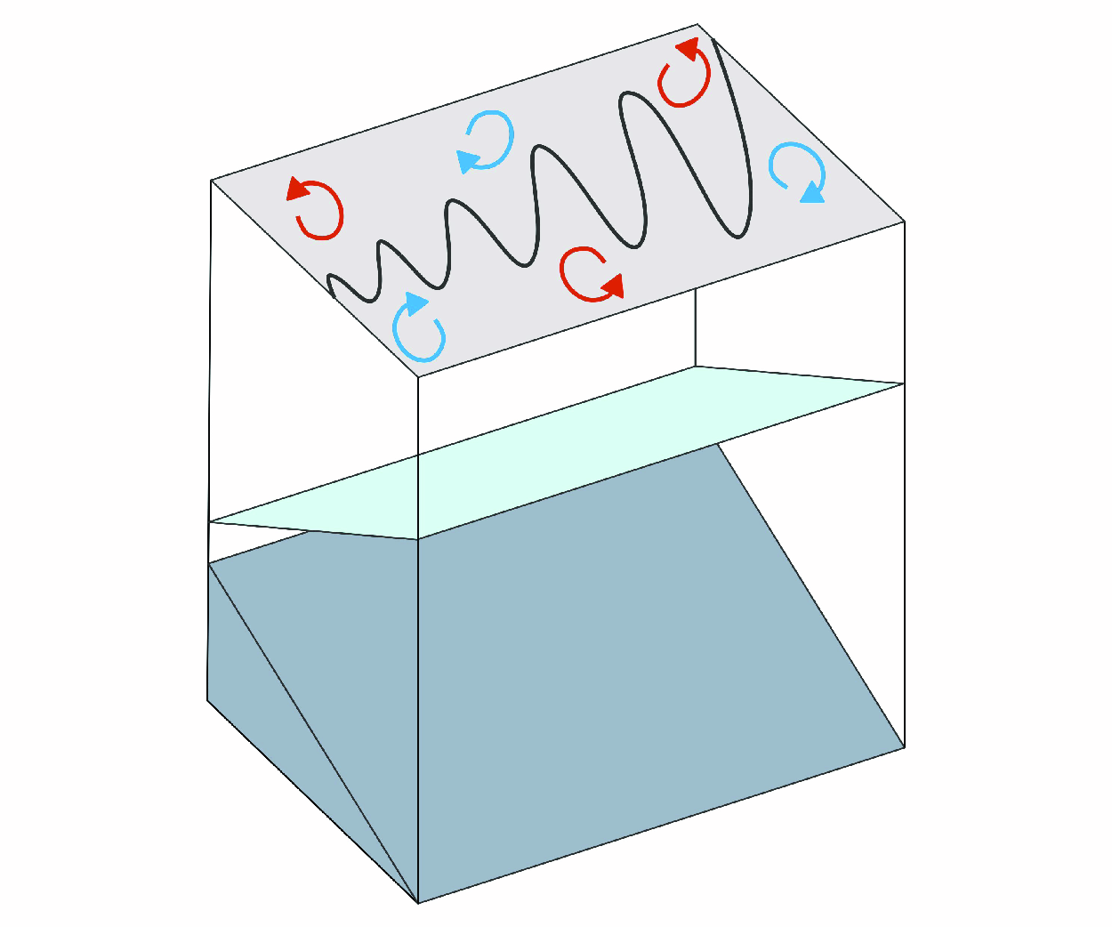
Theoretical quasi-geostrophic (QG) models for baroclinic instability were first developed by Charney (Reference Charney1947) and Eady (Reference Eady1949). Phillips (Reference Phillips1951, Reference Phillips1954) introduced a simplified version: the two-layer QG model. In this model, two fluid layers with homogeneous properties are stacked on top of each other, with different densities and mean flows. The mean flow difference (vertical shear) causes the isopycnal interface between the two layers to tilt due to thermal wind balance. The two-layer QG model incorporates the most important features of baroclinic flows (Flierl Reference Flierl1978). Thus the simplicity and controllability make the model very suitable for studying baroclinic instability, and for linear stability analysis in particular. Although the properties of the fully developed nonlinear eddy field may differ from those predicted by linear stability theory (Early et al. Reference Early, Samelson and Chelton2011; Berloff & Kamenkovich Reference Berloff and Kamenkovich2013a ,Reference Berloff and Kamenkovich b ; Wang et al. Reference Wang, Jansen and Abernathey2016), understanding the linear dynamics can still shed light on the role of different physical properties in the system.
In its most basic version, the two-layer model describes a zonal mean shear on an $f$
-plane over a frictionless flat bottom. However, the model can be modified to include planetary
$f$
-plane over a frictionless flat bottom. However, the model can be modified to include planetary $\beta$
and bottom topography. These both come into the two-layer QG model in the form of potential vorticity (PV) gradients, although they are not dynamically equivalent (Deng & Wang Reference Deng and Wang2024). PV gradients are relevant for eddy dynamics as they suppress eddy mixing (Nakamura & Zhu Reference Nakamura and Zhu2010; Klocker et al. Reference Klocker, Ferrari and LaCasce2012; Sterl et al. Reference Sterl, LaCasce, Groeskamp, Nummelin, Isachsen and Baatsen2024). In the context of linear analysis, both planetary and topographic PV gradients are found to suppress growth rates and stabilise long waves (Blumsack & Gierasch Reference Blumsack and Gierasch1972; Pedlosky Reference Pedlosky1987; Wang et al. Reference Wang, Jansen and Abernathey2016; Leng & Bai Reference Leng and Bai2018). Linear bottom slopes in particular have an important effect: where steep prograde slopes (shear and topographic wave propagation in the same direction, isopycnals and isobaths in opposite directions) only suppress wave growth rates, steep retrograde slopes (shear and topographic wave propagation in opposite directions, isopycnals and isobaths in the same direction) beyond a ‘critical slope’ value stabilise the flow completely, suppressing all baroclinic instability (e.g. Tang Reference Tang1976; Ikeda Reference Ikeda1983; Steinsaltz Reference Steinsaltz1987; Pavec et al. Reference Pavec, Carton and Swaters2005; Poulin & Flierl Reference Poulin and Flierl2005; Chen & Kamenkovich Reference Chen and Kamenkovich2013; LaCasce et al. Reference LaCasce, Escartin, Chassignet and Xu2019). This result follows from the Charney–Stern–Pedlosky criterion, which states that the PV gradient must change sign between the layers for instability to occur (Charney & Stern Reference Charney and Stern1962; Pedlosky Reference Pedlosky1963, Reference Pedlosky1964).
$\beta$
and bottom topography. These both come into the two-layer QG model in the form of potential vorticity (PV) gradients, although they are not dynamically equivalent (Deng & Wang Reference Deng and Wang2024). PV gradients are relevant for eddy dynamics as they suppress eddy mixing (Nakamura & Zhu Reference Nakamura and Zhu2010; Klocker et al. Reference Klocker, Ferrari and LaCasce2012; Sterl et al. Reference Sterl, LaCasce, Groeskamp, Nummelin, Isachsen and Baatsen2024). In the context of linear analysis, both planetary and topographic PV gradients are found to suppress growth rates and stabilise long waves (Blumsack & Gierasch Reference Blumsack and Gierasch1972; Pedlosky Reference Pedlosky1987; Wang et al. Reference Wang, Jansen and Abernathey2016; Leng & Bai Reference Leng and Bai2018). Linear bottom slopes in particular have an important effect: where steep prograde slopes (shear and topographic wave propagation in the same direction, isopycnals and isobaths in opposite directions) only suppress wave growth rates, steep retrograde slopes (shear and topographic wave propagation in opposite directions, isopycnals and isobaths in the same direction) beyond a ‘critical slope’ value stabilise the flow completely, suppressing all baroclinic instability (e.g. Tang Reference Tang1976; Ikeda Reference Ikeda1983; Steinsaltz Reference Steinsaltz1987; Pavec et al. Reference Pavec, Carton and Swaters2005; Poulin & Flierl Reference Poulin and Flierl2005; Chen & Kamenkovich Reference Chen and Kamenkovich2013; LaCasce et al. Reference LaCasce, Escartin, Chassignet and Xu2019). This result follows from the Charney–Stern–Pedlosky criterion, which states that the PV gradient must change sign between the layers for instability to occur (Charney & Stern Reference Charney and Stern1962; Pedlosky Reference Pedlosky1963, Reference Pedlosky1964).
The stabilising effect of steep linear retrograde slopes is a well-studied phenomenon. It is typically studied in the context of an inviscid zonal flow, with all the PV gradients in the system aligned. However, there are also studies that describe the effects of including bottom friction and of varying the orientations of the mean shear and the bottom slope. In this study, we combine all of these effects in a single model to study the instability properties. We review some known results below.
We first consider the relative orientation of the mean shear and the bottom slope. It is known that on the $\beta$
-plane, even a weak non-zonal component of the mean shear can destabilise an otherwise stable system (Kamenkovich & Pedlosky Reference Kamenkovich and Pedlosky1996; Walker & Pedlosky Reference Walker and Pedlosky2002; Arbic & Flierl Reference Arbic and Flierl2004b
; Smith Reference Smith2007a
; Hristova et al. Reference Hristova, Pedlosky and Spall2008). Moreover, even a small zonal slope can destabilise the system (Chen & Kamenkovich Reference Chen and Kamenkovich2013; Khatri & Berloff Reference Khatri and Berloff2018, Reference Khatri and Berloff2019) and increase cross-stream eddy fluxes (Boland et al. Reference Boland, Thompson, Shuckburgh and Haynes2012; Brown et al. Reference Brown, Gulliver and Radko2019). Leng & Bai (Reference Leng and Bai2018) introduced a wavenumber coordinate system to study the baroclinic instability of non-zonal currents. They showed that small differences in the orientation of the mean shear and bottom slope result in different instability characteristics. However, in the case studies that they describe, the bottom slope is still perpendicular to the mean shear. In other words, the topographic and stretching PV gradients are still aligned, though not with the planetary PV gradient.
$\beta$
-plane, even a weak non-zonal component of the mean shear can destabilise an otherwise stable system (Kamenkovich & Pedlosky Reference Kamenkovich and Pedlosky1996; Walker & Pedlosky Reference Walker and Pedlosky2002; Arbic & Flierl Reference Arbic and Flierl2004b
; Smith Reference Smith2007a
; Hristova et al. Reference Hristova, Pedlosky and Spall2008). Moreover, even a small zonal slope can destabilise the system (Chen & Kamenkovich Reference Chen and Kamenkovich2013; Khatri & Berloff Reference Khatri and Berloff2018, Reference Khatri and Berloff2019) and increase cross-stream eddy fluxes (Boland et al. Reference Boland, Thompson, Shuckburgh and Haynes2012; Brown et al. Reference Brown, Gulliver and Radko2019). Leng & Bai (Reference Leng and Bai2018) introduced a wavenumber coordinate system to study the baroclinic instability of non-zonal currents. They showed that small differences in the orientation of the mean shear and bottom slope result in different instability characteristics. However, in the case studies that they describe, the bottom slope is still perpendicular to the mean shear. In other words, the topographic and stretching PV gradients are still aligned, though not with the planetary PV gradient.
Next, we consider the effect of including bottom friction. Numerical models require bottom friction to balance the energy budget and in some cases to limit the inverse energy cascade and thereby achieve realistic levels of mesoscale activity (Arbic & Flierl Reference Arbic and Flierl2004a ; Wang et al. Reference Wang, Jansen and Abernathey2016; Radko et al. Reference Radko, McWilliams and Sutyrin2022). However, bottom friction alters the baroclinic instability properties, in particular destabilising flows that are inviscidly stable. Although bottom friction damps the total eddy energy in the system, it can also increase the eddy available potential energy (APE) while damping the eddy kinetic energy. This in turn increases energy conversion from the background APE to the eddy APE. Thus it is possible that as a net effect, more energy is released than without bottom friction (Lee Reference Lee2010a ). This effect is referred to as ‘dissipative destabilisation’ or ‘frictional instability’, and has been studied using various methods (Holopainen Reference Holopainen1961; Romea Reference Romea1977; Pedlosky Reference Pedlosky1983; Lee & Held Reference Lee and Held1991; Weng & Barcilon Reference Weng and Barcilon1991; Rivière & Klein Reference Rivière and Klein1997; Krechetnikov & Marsden Reference Krechetnikov and Marsden2007, Reference Krechetnikov and Marsden2009; Lee Reference Lee2010a ,Reference Lee b ; Swaters Reference Swaters2010; Willcocks & Esler Reference Willcocks and Esler2012).
However, the joint effect of bottom friction and bottom slopes in the two-layer QG model has received less attention. Weng (Reference Weng1990) discussed the Eady model with a sloping bottom and Ekman layers at both the top and the bottom, and showed that for weak non-zero frictional strength, the critical slope value for instability is extended to a larger value. Swaters (Reference Swaters2009) considered a hybrid planetary geostrophic–QG model, and showed that flows over a sloping bottom are destabilised by a bottom Ekman boundary layer, for any finite Ekman number.
In this study, we transform the two-layer model equations to a wavenumber coordinate system, following Leng & Bai (Reference Leng and Bai2018) but adding bottom friction (§ 2). In § 3, we use the transformed equations to derive instability conditions for a two-layer system with arbitrarily oriented shear and slope. For the inviscid case, we derive a generalised version of the Charney–Stern–Pedlosky criterion, demonstrating the stabilising effect of planetary $\beta$
and steep retrograde slopes for aligned flows (§ 3.1). For non-zero friction, however, the instability condition becomes independent of the bottom slope (§ 3.2). We then study how the instability characteristics – growth rate, wavenumber and propagation direction of the most unstable mode – depend on the orientations of the stretching PV, planetary PV and topographic PV gradients relative to each other, and on the frictional strength (§ 3.3). We conclude and discuss our results in § 4.
$\beta$
and steep retrograde slopes for aligned flows (§ 3.1). For non-zero friction, however, the instability condition becomes independent of the bottom slope (§ 3.2). We then study how the instability characteristics – growth rate, wavenumber and propagation direction of the most unstable mode – depend on the orientations of the stretching PV, planetary PV and topographic PV gradients relative to each other, and on the frictional strength (§ 3.3). We conclude and discuss our results in § 4.
2. Model
2.1. Two-layer model equations
We study a two-layer QG model on a $\beta$
-plane, over a linear bottom slope, with linear bottom friction and forced externally at the surface (e.g. Pedlosky Reference Pedlosky1987; Leng & Bai Reference Leng and Bai2018). We index the upper layer with
$\beta$
-plane, over a linear bottom slope, with linear bottom friction and forced externally at the surface (e.g. Pedlosky Reference Pedlosky1987; Leng & Bai Reference Leng and Bai2018). We index the upper layer with $i=1$
and the lower layer with
$i=1$
and the lower layer with $i=2$
. The two layers have densities
$i=2$
. The two layers have densities $\rho _i$
and thicknesses
$\rho _i$
and thicknesses $H_i$
; the total depth is
$H_i$
; the total depth is $H \equiv H_1 + H_2$
. The total flow field is the sum of a uniform and stationary background field and an eddy field that varies in space and time. We assume that the eddy field is of small amplitude compared to the background field. The background PV is denoted by
$H \equiv H_1 + H_2$
. The total flow field is the sum of a uniform and stationary background field and an eddy field that varies in space and time. We assume that the eddy field is of small amplitude compared to the background field. The background PV is denoted by $Q_{i}$
, and the background flow velocity vector by
$Q_{i}$
, and the background flow velocity vector by $\boldsymbol{U}_i$
. Finally, the eddy PV, eddy flow velocities and eddy streamfunction are denoted by
$\boldsymbol{U}_i$
. Finally, the eddy PV, eddy flow velocities and eddy streamfunction are denoted by $q_i$
,
$q_i$
, $\boldsymbol {u}_i$
and
$\boldsymbol {u}_i$
and $\psi _i$
, respectively. The QG PV equations for the two-layer system are
$\psi _i$
, respectively. The QG PV equations for the two-layer system are
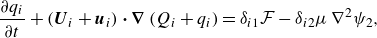 \begin{align} \frac {\partial q_i}{\partial t} + \left (\boldsymbol{U}_i + \boldsymbol{u}_i \right ) \boldsymbol{\cdot} \boldsymbol{\nabla} \left (Q_i+q_i\right ) = \delta _{i1}\mathcal{F} -\delta _{i2}\mu\, \nabla ^2 \psi _2, \end{align}
where $\delta _{ij}$
is the Kronecker delta function,
$\delta _{ij}$
is the Kronecker delta function, $\mathcal{F}$
is the surface forcing, and
$\mathcal{F}$
is the surface forcing, and $\mu$
is the inverse frictional time scale. The eddy PV and velocities are related to the eddy streamfunctions:
$\mu$
is the inverse frictional time scale. The eddy PV and velocities are related to the eddy streamfunctions:
 \begin{align} &q_i = \nabla ^2 \psi _i + (-1)^i F_i \left ( \psi _1 - \psi _2\right ), \end{align}
 \begin{align} &\,\,\quad \boldsymbol{u}_i = \left (-\partial \psi _i/\partial y,\partial \psi _i/\partial x\right ). \end{align}
Here, $F_i$
is the square of the inverse deformation radius in layer
$F_i$
is the square of the inverse deformation radius in layer $i$
, given by
$i$
, given by
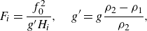 \begin{align} F_i = \frac {f_0^2}{g'H_i}, \quad g' = g \frac {\rho _2 - \rho _1}{\rho _2}, \end{align}
with $f_0$
the Coriolis parameter, and
$f_0$
the Coriolis parameter, and $g'$
the reduced gravity. We write the background velocity in the upper layer as
$g'$
the reduced gravity. We write the background velocity in the upper layer as $\boldsymbol{U}_1 = (U_1,V_1 )$
, and in the lower layer as
$\boldsymbol{U}_1 = (U_1,V_1 )$
, and in the lower layer as $\boldsymbol{U}_2 = (U_2,V_2 )$
. The vertical shears of the zonal and meridional background flow are
$\boldsymbol{U}_2 = (U_2,V_2 )$
. The vertical shears of the zonal and meridional background flow are $\Delta U = U_1 - U_2$
and
$\Delta U = U_1 - U_2$
and $\Delta V = V_1 - V_2$
, respectively. The (linear) bottom slope
$\Delta V = V_1 - V_2$
, respectively. The (linear) bottom slope $\boldsymbol{\alpha } = (\alpha _x, \alpha _y )$
induces a topographic PV gradient
$\boldsymbol{\alpha } = (\alpha _x, \alpha _y )$
induces a topographic PV gradient $\boldsymbol{\nabla} B = ({f_0}/{H_2})\boldsymbol{\alpha }$
in the lower layer. The total background PV gradient is the sum of the stretching, planetary and topographic PV gradients:
$\boldsymbol{\nabla} B = ({f_0}/{H_2})\boldsymbol{\alpha }$
in the lower layer. The total background PV gradient is the sum of the stretching, planetary and topographic PV gradients:
 \begin{align} &\qquad \boldsymbol{\nabla} Q_1 = \left (-F_1\, \Delta V, F_1\, \Delta U + \beta \right ), \end{align}
 \begin{align} &\boldsymbol{\nabla} Q_2 = \left (F_2\, \Delta V + B_x, -F_2\, \Delta U + \beta + B_y \right ). \end{align}
Finally, the term $\boldsymbol{u}_i \boldsymbol{\cdot} \boldsymbol{\nabla} q_i$
in (2.1) represents nonlinear eddy–eddy interactions, which we will ignore in our linear analysis. Thus the linearised versions of (2.1) in terms of the eddy streamfunctions are
$\boldsymbol{u}_i \boldsymbol{\cdot} \boldsymbol{\nabla} q_i$
in (2.1) represents nonlinear eddy–eddy interactions, which we will ignore in our linear analysis. Thus the linearised versions of (2.1) in terms of the eddy streamfunctions are
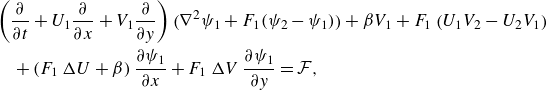 \begin{align} &\qquad \left (\frac {\partial }{\partial t} + U_1 \frac {\partial }{\partial x} + V_1 \frac {\partial }{\partial y} \right ) \bigl(\nabla ^2 \psi _1 + F_1 (\psi _2 - \psi _1 ) \bigr) + \beta V_1 + F_1 \left (U_1V_2 - U_2V_1\right ) \notag\\&\qquad\quad + \left (F_1\, \Delta U + \beta \right )\frac {\partial \psi _1}{\partial x} + F_1\, \Delta V\, \frac {\partial \psi _1}{\partial y} = \mathcal{F}, \end{align}
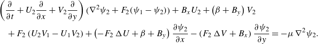 \begin{align} &\left (\frac {\partial }{\partial t} + U_2 \frac {\partial }{\partial x} + V_2 \frac {\partial }{\partial y} \right ) \bigl(\nabla ^2 \psi _2 + F_2 (\psi _1 - \psi _2 ) \bigr) + B_x U_2 + \left (\beta + B_y \right )V_2 \notag\\&\quad + F_2 \left (U_2V_1 - U_1V_2\right ) + \left (-F_2\, \Delta U + \beta + B_y \right )\frac {\partial \psi _2}{\partial x} - \left (F_2\, \Delta V + B_x \right )\frac {\partial \psi _2}{\partial y} = -\mu\, \nabla ^2\psi _2. \end{align}
The lowest-order balance in (2.5a
) is the generalised Sverdrup balance (Sverdrup Reference Sverdrup1947), by which surface forcing ( $\mathcal{F}$
) permits the mean flow to cross the mean PV gradient. There is no forcing in (2.5b
), implying that the mean flow must be parallel to the PV contours. This requires that
$\mathcal{F}$
) permits the mean flow to cross the mean PV gradient. There is no forcing in (2.5b
), implying that the mean flow must be parallel to the PV contours. This requires that
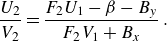 \begin{equation} \frac {U_2}{V_2} = \frac {F_2 U_1 - \beta - B_y}{F_2 V_1 + B_x} \,. \end{equation}
Thus $U_2$
and
$U_2$
and $V_2$
are not independent. We will retain them for now, for generality, but will focus subsequently on the case
$V_2$
are not independent. We will retain them for now, for generality, but will focus subsequently on the case $U_2=V_2=0$
.
$U_2=V_2=0$
.
At next order, (2.5a
) and (2.5b
) become homogeneous equations for the eddy streamfunctions $\psi _i$
(Kamenkovich & Pedlosky Reference Kamenkovich and Pedlosky1996; Leng & Bai Reference Leng and Bai2018). These are the equations on which we will focus:
$\psi _i$
(Kamenkovich & Pedlosky Reference Kamenkovich and Pedlosky1996; Leng & Bai Reference Leng and Bai2018). These are the equations on which we will focus:
 \begin{align} &\left ( \! \frac {\partial }{\partial t} + U_1 \frac {\partial }{\partial x} + V_1 \frac {\partial }{\partial y} \! \right ) \bigl(\nabla ^2 \psi _1 + F_1 (\psi _2 - \psi _1 )\bigr) + \left (F_1\, \Delta U + \beta \right )\! \frac {\partial \psi _1}{\partial x} + F_1\, \Delta V \frac {\partial \psi _1}{\partial y} = 0, \end{align}
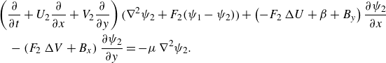 \begin{align} &\quad\left (\frac {\partial }{\partial t} + U_2 \frac {\partial }{\partial x} + V_2 \frac {\partial }{\partial y} \right ) \bigl(\nabla ^2 \psi _2 + F_2 (\psi _1 - \psi _2 ) \bigr) + \left (-F_2\, \Delta U + \beta + B_y \right )\frac {\partial \psi _2}{\partial x} \notag\\&\qquad - \left (F_2\, \Delta V + B_x \right )\frac {\partial \psi _2}{\partial y} = -\mu\, \nabla ^2\psi _2. \end{align}
2.2. Dispersion relation for wave solutions
We look for plane wave solutions of the eddy streamfunctions in a doubly periodic domain:
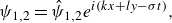 \begin{align} \psi _{1,2} = \hat {\psi }_{1,2} e^{{i}({kx+ly-\sigma t})}, \end{align}
where $\hat {\psi }_{1,2}$
denotes the wave amplitude,
$\hat {\psi }_{1,2}$
denotes the wave amplitude, $\mathbf{K} =(k,l) = \kappa (\cos \theta , \sin \theta )$
is the wavenumber vector, and
$\mathbf{K} =(k,l) = \kappa (\cos \theta , \sin \theta )$
is the wavenumber vector, and $\sigma$
is the angular frequency. The wave phase speed magnitude
$\sigma$
is the angular frequency. The wave phase speed magnitude $c$
is given by
$c$
is given by $c=\sigma /\kappa$
. Substituting (2.8) into (2.7) yields a matrix equation for the wave amplitudes:
$c=\sigma /\kappa$
. Substituting (2.8) into (2.7) yields a matrix equation for the wave amplitudes:
 \begin{align} \begin{pmatrix} M_{11} & M_{12} \\ M_{21} & M_{22} \end{pmatrix} \begin{pmatrix} \hat {\psi }_1 \\ \hat {\psi }_2 \end{pmatrix} = 0, \end{align}
with
 \begin{align} &\qquad\qquad M_{11} = c\kappa \bigl(\kappa ^2 + F_1 \bigr) -\kappa ^2 \left (kU_1+lV_1\right ) - F_1 \left (kU_2+lV_2\right ) + k\beta , \end{align}
 \begin{align} &\qquad\qquad\qquad\qquad\qquad M_{12} = \left (kU_1 + lV_1 - c\kappa \right )F_1, \end{align}
 \begin{align} &\qquad\qquad\qquad\qquad\qquad M_{21} = \left (kU_2 + lV_2 - c\kappa \right )F_2, \end{align}
 \begin{align} & M_{22} = c\kappa \bigl(\kappa ^2 + F_2\bigr) -\kappa ^2 \left (kU_2+lV_2\right ) - F_2 \left (kU_1+lV_1\right ) + k\beta + kB_y - lB_x + i \mu \kappa ^2. \end{align}
To simplify the analysis, we introduce a wavenumber coordinate system, following the approach of Leng & Bai (Reference Leng and Bai2018). In this coordinate system, the unit vectors $\mathbf{e}_\parallel$
and
$\mathbf{e}_\parallel$
and $\mathbf{e}_\perp$
are parallel and perpendicular to
$\mathbf{e}_\perp$
are parallel and perpendicular to $\mathbf{K}$
, respectively. We can then define the following projections:
$\mathbf{K}$
, respectively. We can then define the following projections:
 \begin{align} &\qquad\quad \tilde {U}_i = \frac {\mathbf{K} \boldsymbol{\cdot} \boldsymbol{U}_i}{\kappa } = \frac {kU_i+lV_i}{\kappa } = U_i\cos \theta + V_i\sin \theta , \end{align}
 \begin{align} &\qquad\quad\qquad\quad \hat {\beta } = \frac {\mathbf{K} \times \boldsymbol{\nabla} f}{\kappa } = \frac {k\beta }{\kappa } = \beta \cos \theta , \end{align}
 \begin{align} & \hat {S} = \frac {\mathbf{K} \times \boldsymbol{\nabla} B}{\kappa } = \frac {kB_y - lB_x}{\kappa } = \frac {f_0}{H_2} \left (\alpha _y\cos \theta - \alpha _x\sin \theta \right ) = \frac {f_0}{H_2}\hat {\alpha }, \end{align}
where $\tilde {U}_i$
is the projection of
$\tilde {U}_i$
is the projection of $\boldsymbol{U}_i$
on
$\boldsymbol{U}_i$
on $\mathbf{e}_\parallel$
, and
$\mathbf{e}_\parallel$
, and $\hat {\beta }$
,
$\hat {\beta }$
, $\hat {S}$
and
$\hat {S}$
and $\hat {\alpha }$
are the projections of
$\hat {\alpha }$
are the projections of $\boldsymbol{\nabla} f$
,
$\boldsymbol{\nabla} f$
, $\boldsymbol{\nabla} B$
and
$\boldsymbol{\nabla} B$
and $\boldsymbol{\alpha }$
on
$\boldsymbol{\alpha }$
on $\mathbf{e}_\perp$
, respectively. Thus the projections of the PV gradients on
$\mathbf{e}_\perp$
, respectively. Thus the projections of the PV gradients on $\mathbf{e}_\perp$
are
$\mathbf{e}_\perp$
are
 \begin{align} &\quad\widehat {\boldsymbol{\nabla} Q_1} = F_1\,\Delta \tilde {U} + \hat {\beta }, \end{align}
 \begin{align} &\widehat {\boldsymbol{\nabla} Q_2} = -F_2\,\Delta \tilde {U} + \hat {\beta } + \hat {S}, \end{align}
where $\Delta \tilde {U}=\tilde {U}_1 - \tilde {U}_2$
. The projections (2.11) simplify the matrix equation (2.9) to
$\Delta \tilde {U}=\tilde {U}_1 - \tilde {U}_2$
. The projections (2.11) simplify the matrix equation (2.9) to
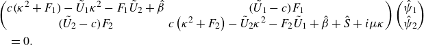 \begin{align} &\begin{pmatrix} c \bigl(\kappa ^2 + F_1 \bigr) - \tilde {U}_1\kappa ^2 - F_1\tilde {U}_2 + \hat {\beta } & \bigl(\tilde {U}_1 - c \bigr)F_1 \\ \bigl(\tilde {U}_2 - c \bigr)F_2 & c\left (\kappa ^2 + F_2\right ) - \tilde {U}_2\kappa ^2 - F_2\tilde {U}_1 + \hat {\beta } + \hat {S} + i \mu \kappa \end{pmatrix} \begin{pmatrix} \hat {\psi }_1 \\ \hat {\psi }_2 \end{pmatrix}\notag\\&\quad = 0. \end{align}
For non-trivial solutions, the determinant of the matrix in (2.13) must be zero. This gives a quadratic equation for $c$
,
$c$
, $A_1 c^2 + A_2 c + A_3 = 0$
, which has the following solution:
$A_1 c^2 + A_2 c + A_3 = 0$
, which has the following solution:
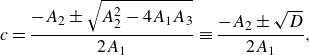 \begin{align} &\qquad\qquad\qquad c = \frac {-A_2 \pm \sqrt {A_2^2-4A_1A_3}}{2A_1} \equiv \frac {-A_2 \pm \sqrt {D}}{2A_1},\\[-8pt]\nonumber \end{align}
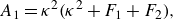 \begin{align} &\qquad\qquad\qquad\qquad\quad A_1 = \kappa ^2 \bigl(\kappa ^2 + F_1 + F_2 \bigr),\\[-8pt]\nonumber \end{align}
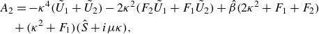 \begin{align} & A_2 = -\kappa ^4\bigl(\tilde {U}_1 + \tilde {U}_2\bigr) - 2\kappa ^2\bigl(F_2\tilde {U}_1 +F_1\tilde {U}_2\bigr) + \hat {\beta } \bigl(2\kappa ^2 + F_1 + F_2 \bigr)\notag\\&\quad + \bigl(\kappa ^2 + F_1 \bigr) \bigl(\hat {S} + i \mu \kappa \bigr),\\[-8pt]\nonumber \end{align}
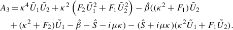 \begin{align} &A_3 = \kappa ^4 \tilde {U}_1\tilde {U}_2 + \kappa ^2 \left (F_2\tilde {U}_1^2 +F_1\tilde {U}_2^2\right ) - \hat {\beta } \biggl(\bigl(\kappa ^2 + F_1 \bigr) \tilde {U}_2 \notag\\& \quad +\bigl(\kappa ^2 + F_2 \bigr) \tilde {U}_1 - \hat {\beta } - \hat {S} - i \mu \kappa \biggr) - \bigl(\hat {S} + i \mu \kappa \bigr) \Bigl(\kappa ^2 \tilde {U}_1 + F_1 \tilde {U}_2 \Bigr). \end{align}
The solution for $c$
can have both a real part and an imaginary part. The real part,
$c$
can have both a real part and an imaginary part. The real part, $c_r$
, denotes the eddy phase speed. The imaginary part,
$c_r$
, denotes the eddy phase speed. The imaginary part, $c_i$
, multiplied by the wavenumber magnitude, denotes the unstable growth rate,
$c_i$
, multiplied by the wavenumber magnitude, denotes the unstable growth rate, $\sigma _i = \kappa c_i$
. The requirement for baroclinic instability is that
$\sigma _i = \kappa c_i$
. The requirement for baroclinic instability is that $\sigma _i \gt 0$
.
$\sigma _i \gt 0$
.
3. Linear stability analysis
3.1. Instability conditions in inviscid case
We can use the dispersion relation (2.14) to study the instability of the two-layer model. We start by considering the inviscid case ( $\mu = 0$
). In this case, a necessary and sufficient condition for instability is that
$\mu = 0$
). In this case, a necessary and sufficient condition for instability is that $D = A_2^2 - 4A_1A_3$
in (2.14a
) is negative (as
$D = A_2^2 - 4A_1A_3$
in (2.14a
) is negative (as $A_1,A_2,A_3$
are all real,
$A_1,A_2,A_3$
are all real, $\sqrt {D}$
is the only possible source of an imaginary part of
$\sqrt {D}$
is the only possible source of an imaginary part of $c$
). Here,
$c$
). Here, $D$
is a polynomial in
$D$
is a polynomial in $\kappa$
, and from
$\kappa$
, and from $D\lt 0$
it follows that there exist both a long-wave and a short-wave cut-off for instability. To get insight into the role of the bottom slope, we derive another necessary condition for instability. We multiply the first row of (2.13) by
$D\lt 0$
it follows that there exist both a long-wave and a short-wave cut-off for instability. To get insight into the role of the bottom slope, we derive another necessary condition for instability. We multiply the first row of (2.13) by $d_1 \hat {\kern-1pt \psi}_{1}^\ast / (c-\tilde {U}_1 )$
and the second row by
$d_1 \hat {\kern-1pt \psi}_{1}^\ast / (c-\tilde {U}_1 )$
and the second row by $d_2\hat {\kern-1pt \psi}_{2}^\ast / (c-\tilde {U}_2 )$
, where
$d_2\hat {\kern-1pt \psi}_{2}^\ast / (c-\tilde {U}_2 )$
, where $d_i \equiv H_i/H$
, and
$d_i \equiv H_i/H$
, and $\ast$
denotes the complex conjugate. Next, we sum the two rows and find
$\ast$
denotes the complex conjugate. Next, we sum the two rows and find
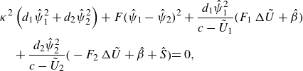 \begin{align} &\kappa ^2 \left (d_1 \hat {\psi }_1^2 + d_2 \hat {\psi }_2^2 \right ) + F \bigl(\hat {\psi }_1 - \hat {\psi }_2 \bigr)^2 + \frac {d_1 \hat {\psi }_1^2}{c-\tilde {U}_1} \bigl(F_1\, \Delta \tilde {U} + \hat {\beta } \bigr)\notag\\&\quad + \frac {d_2 \hat {\psi }_2^2}{c-\tilde {U}_2} \bigr(-F_2\, \Delta \tilde {U} + \hat {\beta } + \hat {S} \bigl) = 0, \end{align}
where $F \equiv f_0^2/ (g'H )$
. Both the real and imaginary part of (3.1) must vanish separately. The imaginary part of (3.1) is
$F \equiv f_0^2/ (g'H )$
. Both the real and imaginary part of (3.1) must vanish separately. The imaginary part of (3.1) is
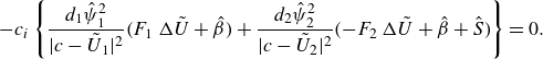 \begin{align} -c_i \left \lbrace \frac {d_1 \hat {\psi }_1^2}{|c-\tilde {U}_1|^2} \bigl(F_1\, \Delta \tilde {U} + \hat {\beta } \bigr) + \frac {d_2 \hat {\psi }_2^2}{|c-\tilde {U}_2|^2} \bigl(-F_2\, \Delta \tilde {U} + \hat {\beta } + \hat {S} \bigr) \right \rbrace = 0. \end{align}
For $c_i \neq 0$
, which is necessary for instability, (3.2) implies that
$c_i \neq 0$
, which is necessary for instability, (3.2) implies that
 \begin{align} \bigl( F_1\, \Delta \tilde {U} + \hat {\beta } \bigr) \bigl( -F_2\,\Delta \tilde {U} + \hat {\beta } + \hat {S} \bigr) \lt 0. \end{align}
Note that (3.3) is equivalent to $\widehat {\boldsymbol{\nabla} Q_1}\, \widehat {\boldsymbol{\nabla} Q_2} \lt 0$
. In other words, the component of the PV gradient perpendicular to the wavenumber vector must change sign between the layers for the flow to be unstable. This is the generalisation of the Charney–Stern–Pedlosky criterion (Charney & Stern Reference Charney and Stern1962; Pedlosky Reference Pedlosky1963, Reference Pedlosky1964). A number of interesting aspects emerge from the instability condition (3.3). First, the relevant parameter for stability is the vertical velocity shear
$\widehat {\boldsymbol{\nabla} Q_1}\, \widehat {\boldsymbol{\nabla} Q_2} \lt 0$
. In other words, the component of the PV gradient perpendicular to the wavenumber vector must change sign between the layers for the flow to be unstable. This is the generalisation of the Charney–Stern–Pedlosky criterion (Charney & Stern Reference Charney and Stern1962; Pedlosky Reference Pedlosky1963, Reference Pedlosky1964). A number of interesting aspects emerge from the instability condition (3.3). First, the relevant parameter for stability is the vertical velocity shear $\Delta \tilde {U}$
rather than the individual layer velocities. Also, planetary PV has a stabilising effect since sufficiently large
$\Delta \tilde {U}$
rather than the individual layer velocities. Also, planetary PV has a stabilising effect since sufficiently large $\hat {\beta }$
will make both
$\hat {\beta }$
will make both $\widehat {\boldsymbol{\nabla} Q_1}$
and
$\widehat {\boldsymbol{\nabla} Q_1}$
and $\widehat {\boldsymbol{\nabla} Q_2}$
positive. Note that for meridional wavenumber vectors (
$\widehat {\boldsymbol{\nabla} Q_2}$
positive. Note that for meridional wavenumber vectors ( $\theta = \unicode{x03C0} /2$
or
$\theta = \unicode{x03C0} /2$
or $3\unicode{x03C0} /2$
), planetary PV cannot stabilise the flow, as
$3\unicode{x03C0} /2$
), planetary PV cannot stabilise the flow, as $\hat {\beta } = 0$
then. Finally, it follows from (3.3) that there exists a critical slope for instability:
$\hat {\beta } = 0$
then. Finally, it follows from (3.3) that there exists a critical slope for instability:
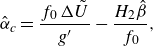 \begin{align} \hat {\alpha }_c = \frac {f_0\, \Delta \tilde {U}}{g'} - \frac {H_2\hat {\beta }}{f_0}, \end{align}
with the necessary instability conditions
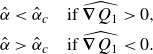 \begin{align} \hat {\alpha } &\lt \hat {\alpha }_c \quad \text{if } \widehat {\boldsymbol{\nabla} Q_1} \gt 0,\notag\\ \hat {\alpha } &\gt \hat {\alpha }_c \quad \text{if } \widehat {\boldsymbol{\nabla} Q_1} \lt 0. \end{align}
Thus if the bottom slope component perpendicular to $\mathbf{K}$
exceeds the critical slope, then there is no instability for wavenumber vectors with wave angle
$\mathbf{K}$
exceeds the critical slope, then there is no instability for wavenumber vectors with wave angle $\theta$
. (Here, ‘exceeds’ can mean either to be smaller or greater, depending on the sign of
$\theta$
. (Here, ‘exceeds’ can mean either to be smaller or greater, depending on the sign of $\widehat {\boldsymbol{\nabla} Q_1}$
.) The term
$\widehat {\boldsymbol{\nabla} Q_1}$
.) The term $f_0\,\Delta \tilde {U}/g'$
on the right-hand side of (3.4) represents the slope of the density interface between the two layers, projected on
$f_0\,\Delta \tilde {U}/g'$
on the right-hand side of (3.4) represents the slope of the density interface between the two layers, projected on $\mathbf{e}_\parallel$
. This means that on the
$\mathbf{e}_\parallel$
. This means that on the $f$
-plane, the instability condition (3.5) is that the bottom slope component perpendicular to
$f$
-plane, the instability condition (3.5) is that the bottom slope component perpendicular to $\mathbf{K}$
is less steep than the isopycnal slope component parallel to
$\mathbf{K}$
is less steep than the isopycnal slope component parallel to $\mathbf{K}$
. Again, this is a generalisation of a well-known result for zonal flows (e.g. Blumsack & Gierasch Reference Blumsack and Gierasch1972; Mechoso Reference Mechoso1980; Pavec et al. Reference Pavec, Carton and Swaters2005; Isachsen Reference Isachsen2011; Pennel & Kamenkovich Reference Pennel and Kamenkovich2014). Note that (3.5) is not a sufficient condition for instability; as mentioned above, for slopes below the critical slope, there is still instability only for a limited range of wavenumber magnitudes.
$\mathbf{K}$
. Again, this is a generalisation of a well-known result for zonal flows (e.g. Blumsack & Gierasch Reference Blumsack and Gierasch1972; Mechoso Reference Mechoso1980; Pavec et al. Reference Pavec, Carton and Swaters2005; Isachsen Reference Isachsen2011; Pennel & Kamenkovich Reference Pennel and Kamenkovich2014). Note that (3.5) is not a sufficient condition for instability; as mentioned above, for slopes below the critical slope, there is still instability only for a limited range of wavenumber magnitudes.
3.2. Instability condition with bottom friction
If $\mu \neq 0$
, then the situation changes, as both
$\mu \neq 0$
, then the situation changes, as both $A_2$
and
$A_2$
and $A_3$
in (2.14) have an imaginary part. As seen in the dispersion relation (2.14), including bottom friction is equivalent to adding an imaginary part to the slope parameter
$A_3$
in (2.14) have an imaginary part. As seen in the dispersion relation (2.14), including bottom friction is equivalent to adding an imaginary part to the slope parameter $\hat S$
. The imaginary part of
$\hat S$
. The imaginary part of $c$
is now given by
$c$
is now given by
 \begin{align} c_i = \frac {{\textrm {Im}}(-A_2) \pm {\textrm {Im}}(\sqrt {D})}{2A_1}. \end{align}
The necessary and sufficient condition for instability is that (3.6) is positive. The imaginary part of $-A_2$
is equal to
$-A_2$
is equal to $- (\kappa ^2 + F_1 )\mu \kappa$
. To get an expression for the imaginary part of
$- (\kappa ^2 + F_1 )\mu \kappa$
. To get an expression for the imaginary part of $\sqrt {D}$
, we first write
$\sqrt {D}$
, we first write $D$
in polar coordinates:
$D$
in polar coordinates:
 \begin{align} D = r\,{\textrm e}^{{i}\gamma } \implies \sqrt {D} = \sqrt {r}\,{\textrm e}^{{i}\left (\gamma /2 + n\unicode{x03C0} \right )}, \quad n=0,1. \end{align}
The $n=0$
solution of (3.7) corresponds to a positive
$n=0$
solution of (3.7) corresponds to a positive ${\textrm {Im}} (\sqrt {D} )$
, while the
${\textrm {Im}} (\sqrt {D} )$
, while the $n=1$
solution yields a negative value. Thus instability implies the sum in (3.6) with
$n=1$
solution yields a negative value. Thus instability implies the sum in (3.6) with $n=0$
, and the difference with
$n=0$
, and the difference with $n=1$
. In either case, the condition for instability reduces to
$n=1$
. In either case, the condition for instability reduces to
 \begin{align} \sqrt {r} \sin \left (\gamma /2\right ) \gt \bigl(\kappa ^2 + F_1 \bigr)\mu \kappa . \end{align}
We use the half-angle formula to rewrite the instability condition as (see also Swaters Reference Swaters2009, Reference Swaters2010)
 \begin{align} 2r \sin ^2(\gamma /2) = r\left (1-\cos \gamma \right ) \gt 2\bigl(\kappa ^2 + F_1 \bigr)^2\mu ^2\kappa ^2, \end{align}
or equivalently,
 \begin{align} \sqrt {{\textrm {Re}}(D)^2+{\textrm {Im}}(D)^2} \gt {\textrm {Re}}(D) + 2\bigl(\kappa ^2 + F_1 \bigr)^2\mu ^2\kappa ^2. \end{align}
Squaring both sides yields
 \begin{align} {\textrm {Im}}(D)^2 \gt 4\bigl(\kappa ^2 + F_1 \bigr)^2\mu ^2\kappa ^2\,{\textrm {Re}}(D) + 4\bigl(\kappa ^2 + F_1 \bigr)^4\mu ^4\kappa ^4. \end{align}
We obtain ${\textrm {Re}}(D)$
and
${\textrm {Re}}(D)$
and ${\textrm {Im}}(D)$
from
${\textrm {Im}}(D)$
from $D = A_2^2-4A_1A_3$
following (2.14). Some tedious but straightforward algebra yields the following expressions:
$D = A_2^2-4A_1A_3$
following (2.14). Some tedious but straightforward algebra yields the following expressions:
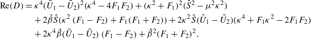 \begin{align} {\textrm {Re}}(D) & = \kappa ^4 \bigl(\tilde {U}_1 - \tilde {U}_2 \bigr)^2 \bigl(\kappa ^4 - 4F_1F_2 \bigr) + \bigl(\kappa ^2+F_1\bigr)^2 \Bigl(\hat {S}^2 - \mu ^2\kappa ^2 \Bigr) \notag\\&\quad + 2\hat {\beta }\hat {S} \bigl(\kappa ^2 \left (F_1 - F_2 \right ) + F_1 (F_1 + F_2 ) \bigr) + 2\kappa ^2\hat {S} \bigl(\tilde {U}_1 - \tilde {U}_2 \bigr) \Bigl(\kappa ^4 + F_1\kappa ^2 - 2F_1F_2 \Bigr) \notag\\&\quad + 2\kappa ^4\hat {\beta } \bigl(\tilde {U}_1 - \tilde {U}_2 \bigr) \left (F_1-F_2\right ) + \hat {\beta }^2 (F_1 + F_2 )^2, \end{align}
 \begin{align} {\textrm {Im}}(D) & = 2\hat {S} \mu \kappa \bigl(\kappa ^2 + F_1 \bigr)^2 + 2\mu \kappa ^3 \bigl(\tilde {U}_1 - \tilde {U}_2 \bigr)\Bigl(\kappa ^4 + F_1\kappa ^2 - 2F_1F_2 \Bigr) \notag\\&\quad + 2\hat {\beta }\mu \kappa \bigl(\kappa ^2 \left (F_1 - F_2 \right ) + F_1 (F_1 + F_2 ) \bigr). \end{align}
Again, only the vertical velocity shear $\Delta \tilde {U} = \tilde {U}_1 - \tilde {U}_2$
enters the expression. Substituting (3.12) in (3.11) leads eventually to many terms cancelling out. Most notably, all terms containing the bottom slope term
$\Delta \tilde {U} = \tilde {U}_1 - \tilde {U}_2$
enters the expression. Substituting (3.12) in (3.11) leads eventually to many terms cancelling out. Most notably, all terms containing the bottom slope term $\hat {S}$
disappear. Thus the slope can no longer stabilise the flow in the presence of a bottom Ekman layer. Finally, (3.11) reduces to
$\hat {S}$
disappear. Thus the slope can no longer stabilise the flow in the presence of a bottom Ekman layer. Finally, (3.11) reduces to
 \begin{align} 16\kappa ^4 F_1 F_2 \mu ^2 \bigl(\kappa ^2 + F_1 + F_2\bigr) \bigl(\Delta \tilde {U}\,\kappa ^2-\hat {\beta }\bigr) \bigl(F_1\, \Delta \tilde {U}+\hat {\beta } \bigr) \gt 0. \end{align}
The first portion is always positive, so for the $\mu \neq 0$
case, there is instability if and only if
$\mu \neq 0$
case, there is instability if and only if
 \begin{align} \bigl(\Delta \tilde {U}\,\kappa ^2-\hat {\beta }\bigr) \bigl(F_1\, \Delta \tilde {U}+\hat {\beta } \bigr) \gt 0. \end{align}
Thus there can be instability only if $\Delta \tilde {U}$
is non-zero. A further constraint that is necessary and sufficient for instability follows from (3.14), depending on the sign of
$\Delta \tilde {U}$
is non-zero. A further constraint that is necessary and sufficient for instability follows from (3.14), depending on the sign of $\Delta \tilde {U} \boldsymbol{\cdot} \hat {\beta }$
:
$\Delta \tilde {U} \boldsymbol{\cdot} \hat {\beta }$
:
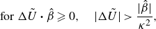 \begin{align} &\text{for } \Delta \tilde {U} \boldsymbol{\cdot} \hat {\beta } \geqslant 0, \quad |\Delta \tilde {U}| \gt \frac {|\hat {\beta }|}{\kappa ^2}, \end{align}
 \begin{align} &\text{for } \Delta \tilde {U} \boldsymbol{\cdot} \hat {\beta } \leqslant 0, \quad |\Delta \tilde {U}| \gt \frac {|\hat {\beta }|}{F_1}. \end{align}
So there is a critical shear for instability; as long as $\Delta \tilde {U}$
is greater than this critical shear, the system is unstable for all wave orientations
$\Delta \tilde {U}$
is greater than this critical shear, the system is unstable for all wave orientations $\theta$
. If
$\theta$
. If $\Delta \tilde {U}$
and
$\Delta \tilde {U}$
and $\hat {\beta }$
have equal signs, then the critical shear is determined by the planetary PV gradient and the wavenumber, and long waves are stable. If
$\hat {\beta }$
have equal signs, then the critical shear is determined by the planetary PV gradient and the wavenumber, and long waves are stable. If $\Delta \tilde {U}$
and
$\Delta \tilde {U}$
and $\hat {\beta }$
have opposite signs, then the critical shear depends on the planetary PV gradient and the upper layer deformation radius, and there is no constraint for the wavenumber magnitude. The instability is thus no longer confined to a wavenumber range with both a long-wave and short-wave cut-off, as in the inviscid case; friction destabilises the system (e.g. Holopainen Reference Holopainen1961). Planetary PV can stabilise the flow; on an
$\hat {\beta }$
have opposite signs, then the critical shear depends on the planetary PV gradient and the upper layer deformation radius, and there is no constraint for the wavenumber magnitude. The instability is thus no longer confined to a wavenumber range with both a long-wave and short-wave cut-off, as in the inviscid case; friction destabilises the system (e.g. Holopainen Reference Holopainen1961). Planetary PV can stabilise the flow; on an $f$
-plane, or for meridional wave vectors (
$f$
-plane, or for meridional wave vectors ( $\hat {\beta }=0$
), there is instability for all non-zero
$\hat {\beta }=0$
), there is instability for all non-zero $\Delta \tilde {U}$
at wave angle
$\Delta \tilde {U}$
at wave angle $\theta$
. Notably, neither the friction coefficient
$\theta$
. Notably, neither the friction coefficient $\mu$
nor the bottom slope
$\mu$
nor the bottom slope $\hat {\alpha }$
appear in the instability condition (3.14). Frictional destabilisation happens even for infinitesimally small frictional strength, consistent with Swaters (Reference Swaters2009, Reference Swaters2010). Moreover, as long as (3.14) holds, the flow is unstable for all slopes, irrespective of magnitude or orientation. Interestingly, (3.14) also holds for unstable flows in the inviscid case (this follows from combining (3.3) with
$\hat {\alpha }$
appear in the instability condition (3.14). Frictional destabilisation happens even for infinitesimally small frictional strength, consistent with Swaters (Reference Swaters2009, Reference Swaters2010). Moreover, as long as (3.14) holds, the flow is unstable for all slopes, irrespective of magnitude or orientation. Interestingly, (3.14) also holds for unstable flows in the inviscid case (this follows from combining (3.3) with $A_3\gt 0$
, which must be true for
$A_3\gt 0$
, which must be true for $D\lt 0$
). However, (3.14) is not sufficient for instability in an inviscid system; constraints for the wavenumber magnitude and slope must be met. By contrast, for
$D\lt 0$
). However, (3.14) is not sufficient for instability in an inviscid system; constraints for the wavenumber magnitude and slope must be met. By contrast, for $\mu \neq 0$
, (3.14) is necessary and sufficient for instability. The inviscid case is thus a singular limit of the two-layer model.
$\mu \neq 0$
, (3.14) is necessary and sufficient for instability. The inviscid case is thus a singular limit of the two-layer model.
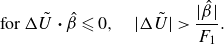
Growth rate of unstable waves as a function of wavenumber (normalised by the deformation wavenumber) for different frictional time scales, with parameters as in (3.16). Note the different colour bar ranges. The black curve in each plot shows the wavenumber that maximises the growth rate as a function of the bottom slope.
The impact of bottom slope and bottom friction on baroclinic instability is visualised in figure 1, which shows the growth rates of unstable waves as a function of wavenumber. For this figure, we consider a zonal mean shear and a meridional bottom slope, so that the planetary, topographic and stretching PV are all aligned, even without the transformation to wavenumber coordinates. We consider a zonal wavenumber vector ( $\theta = 0$
) as this always yields the maximum growth rate. The following dimensional parameters are used, which are representative values for the ocean (e.g. Dohan & Maximenko Reference Dohan and Maximenko2010; Koltermann et al. Reference Koltermann, Gouretski and Jancke2011; LaCasce & Groeskamp Reference LaCasce and Groeskamp2020):
$\theta = 0$
) as this always yields the maximum growth rate. The following dimensional parameters are used, which are representative values for the ocean (e.g. Dohan & Maximenko Reference Dohan and Maximenko2010; Koltermann et al. Reference Koltermann, Gouretski and Jancke2011; LaCasce & Groeskamp Reference LaCasce and Groeskamp2020):
 \begin{align} &\qquad\qquad f_0 = 10^{-4} \ \textrm{s}^{-1}, \quad \beta = 10^{-11} \ \textrm{m}^{-1}\ \textrm{s}^{-1}, \quad \Delta U = 0.04 \ \textrm{m s}^{-1},\notag \\ &H_1 = 1000 \ \textrm{m}, \quad H_2 = 4000 \ \textrm{m},\quad \rho _1 = 1027.5 \ \textrm{kg m}^{-3},\quad \rho _2 = 1028 \ \textrm{kg m}^{-3}. \end{align}
In this configuration, the deformation radius $L_d = 1/\kappa _d = 1/\sqrt {F_1+F_2}$
is 20 km, and the upper layer deformation radius
$L_d = 1/\kappa _d = 1/\sqrt {F_1+F_2}$
is 20 km, and the upper layer deformation radius $L_{d1} = 1/\sqrt {F_1}$
is 22 km. As estimates of the inverse frictional time scale
$L_{d1} = 1/\sqrt {F_1}$
is 22 km. As estimates of the inverse frictional time scale $\mu ^{-1}$
in the ocean are of the order of 1–100 day
$\mu ^{-1}$
in the ocean are of the order of 1–100 day $^{-1}$
(Arbic & Flierl Reference Arbic and Flierl2004a
), we test different orders of magnitude of
$^{-1}$
(Arbic & Flierl Reference Arbic and Flierl2004a
), we test different orders of magnitude of $\mu$
. Furthermore, we test bottom slope magnitudes of the order of
$\mu$
. Furthermore, we test bottom slope magnitudes of the order of $10^{-4}{-}10^{-3}$
, which capture most of the open ocean (LaCasce Reference LaCasce2017). As we consider an eastward mean shear in the Northern Hemisphere, positive slopes (rising towards the north) are retrograde, and negative slopes are prograde in this configuration. Figure 1(a) demonstrates the existence of a critical slope for instability in the inviscid case, resulting in a strong asymmetry between retrograde and prograde slopes (Blumsack & Gierasch Reference Blumsack and Gierasch1972; Mechoso Reference Mechoso1980). Figure 1(b) shows that even weak bottom friction destabilises the system for all bottom slopes, and removes the short-wave cut-offs (as
$10^{-4}{-}10^{-3}$
, which capture most of the open ocean (LaCasce Reference LaCasce2017). As we consider an eastward mean shear in the Northern Hemisphere, positive slopes (rising towards the north) are retrograde, and negative slopes are prograde in this configuration. Figure 1(a) demonstrates the existence of a critical slope for instability in the inviscid case, resulting in a strong asymmetry between retrograde and prograde slopes (Blumsack & Gierasch Reference Blumsack and Gierasch1972; Mechoso Reference Mechoso1980). Figure 1(b) shows that even weak bottom friction destabilises the system for all bottom slopes, and removes the short-wave cut-offs (as $\Delta U \boldsymbol{\cdot} \beta \gt 0$
here, there is still a long-wave cut-off at
$\Delta U \boldsymbol{\cdot} \beta \gt 0$
here, there is still a long-wave cut-off at $\kappa = \sqrt {\beta /\Delta U}$
; see (3.15)), but also that the growth rates become weaker. There is still strong asymmetry between retrograde and prograde slopes: for retrograde slopes, growth rates are much weaker, and the maximum growth occurs at smaller wavenumbers than for prograde slopes. With increasing frictional strength (figure 1
c,d), the growth rates decrease further, and the asymmetry between retrograde and prograde slopes gets weaker. Thus there is a shift from a slope-dominated regime to a friction-dominated regime. This can be understood from (2.14) by noting that the terms representing the topographic PV gradient and the bottom friction always appear together as the sum
$\kappa = \sqrt {\beta /\Delta U}$
; see (3.15)), but also that the growth rates become weaker. There is still strong asymmetry between retrograde and prograde slopes: for retrograde slopes, growth rates are much weaker, and the maximum growth occurs at smaller wavenumbers than for prograde slopes. With increasing frictional strength (figure 1
c,d), the growth rates decrease further, and the asymmetry between retrograde and prograde slopes gets weaker. Thus there is a shift from a slope-dominated regime to a friction-dominated regime. This can be understood from (2.14) by noting that the terms representing the topographic PV gradient and the bottom friction always appear together as the sum $\hat {S} + i \mu \kappa$
; as
$\hat {S} + i \mu \kappa$
; as $\mu$
increases, so does its relative importance over the topographic term.
$\mu$
increases, so does its relative importance over the topographic term.
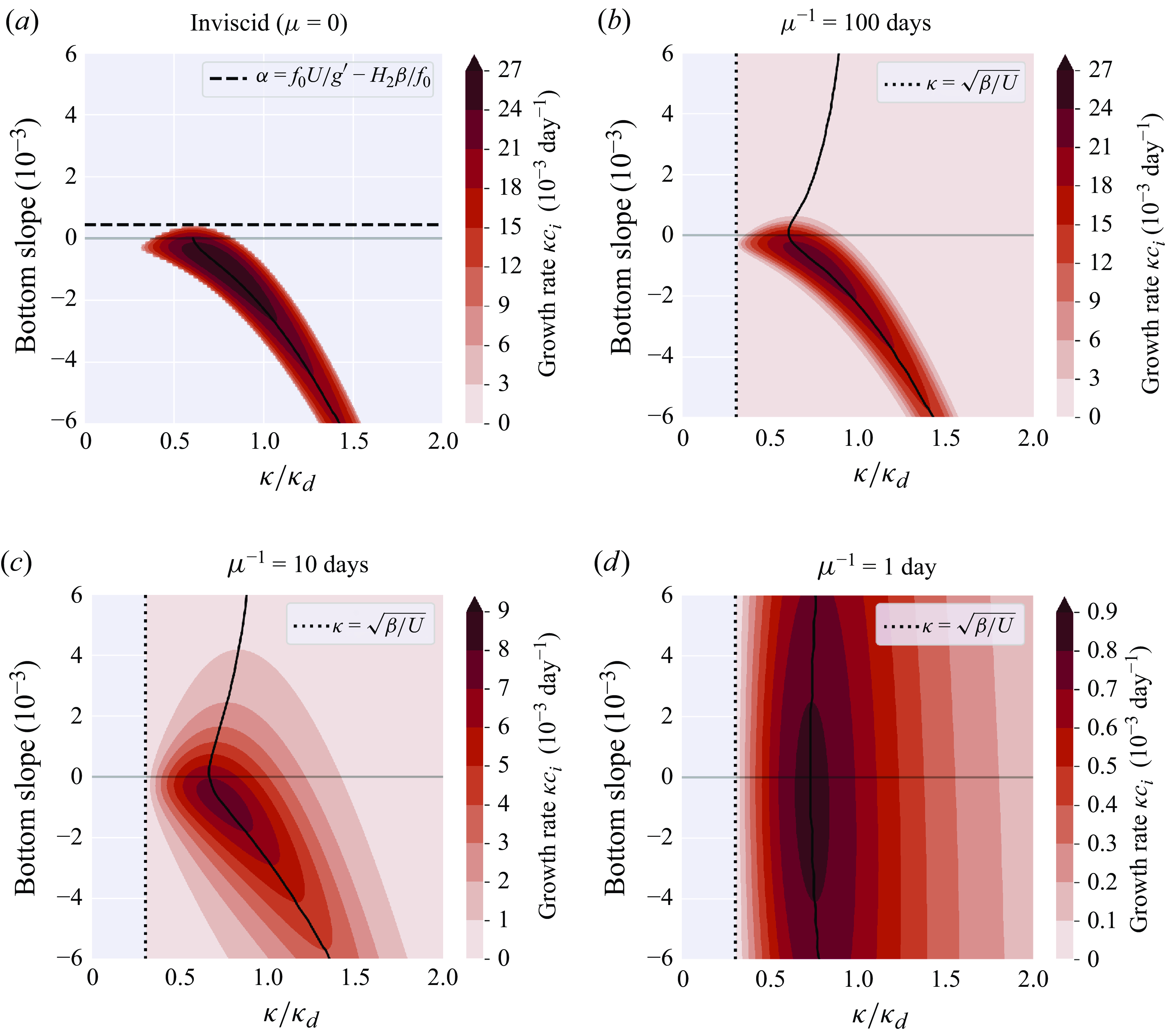
Figure 2 shows the maximum growth rate as a function of bottom slope, for both positive and negative zonal shear configurations. For no or weak friction, the most unstable growth rate depends strongly and asymmetrically on the bottom slope. The growth rates are much higher for prograde slopes than for retrograde slopes in this parameter configuration. For stronger, but realistic friction, the growth rate curves flatten, illustrating the shift from the slope-dominated regime to the friction-dominated regime. The growth rates are very low for strong friction. Hence even though the system is unstable in an analytical sense, the unstable modes grow only very slowly for strong friction.
The maximum growth rate as a function of the bottom slope for different frictional strengths, for positive zonal shear $\Delta U = 0.04 \ {\textrm{m s}}^{-1}$
and negative zonal shear
$\Delta U = 0.04 \ {\textrm{m s}}^{-1}$
and negative zonal shear $\Delta U = -0.04 \ {\textrm{m s}}^{-1}$
, and the other model parameters as in (3.16).
$\Delta U = -0.04 \ {\textrm{m s}}^{-1}$
, and the other model parameters as in (3.16).
3.3. Instability characteristics for varying orientations of the PV gradients
We now consider how the instability characteristics of the two-layer model change for varying orientations of the mean shear and the topography. For simplicity, we set $\boldsymbol{U}_2 = 0$
so that the shear vector is
$\boldsymbol{U}_2 = 0$
so that the shear vector is $\boldsymbol{U}_1 \equiv \boldsymbol{U}$
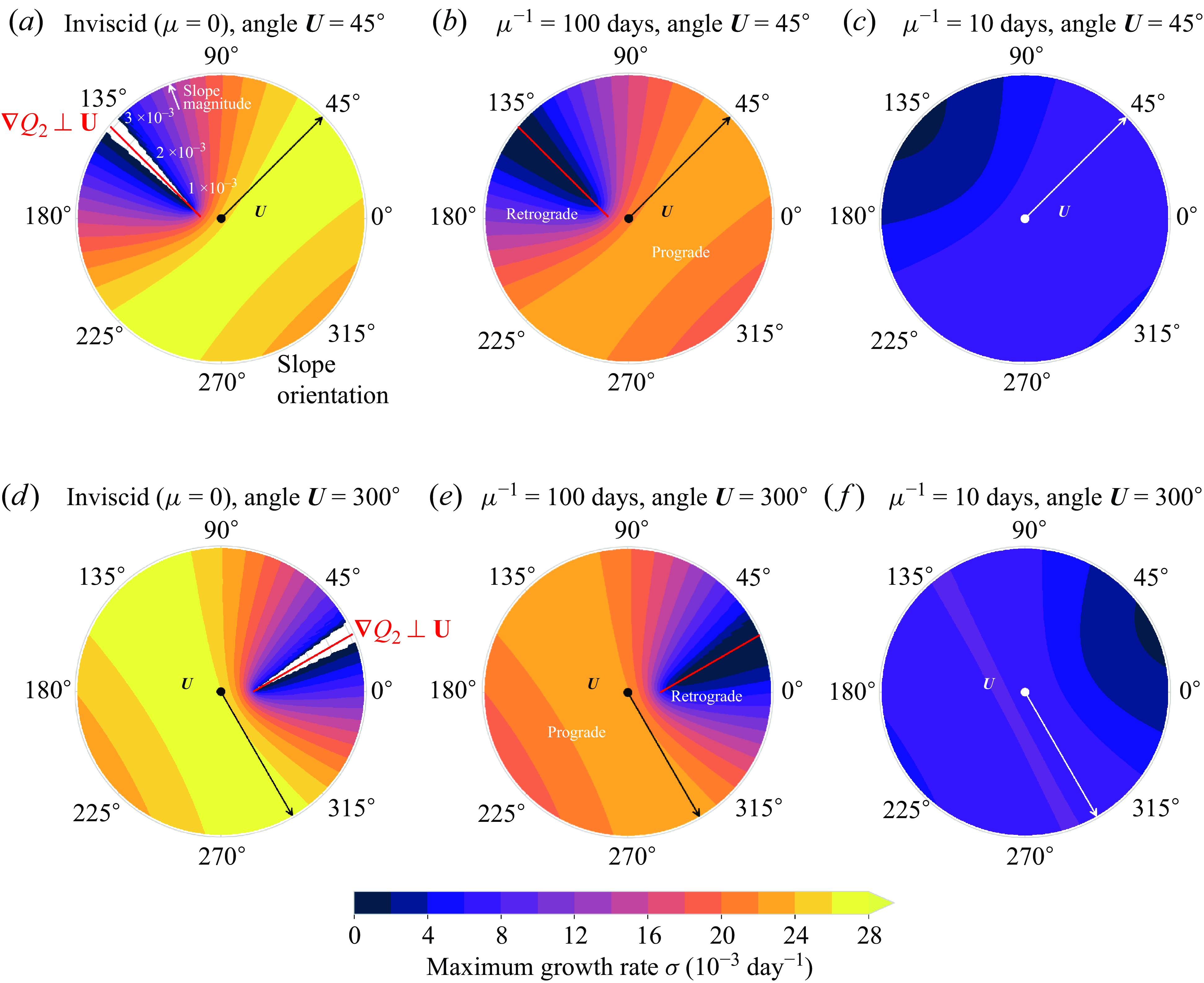
. Figure 3 shows the most unstable growth rate as a function of the bottom slope vector, for shear vectors making angles
$\boldsymbol{U}_1 \equiv \boldsymbol{U}$
. Figure 3 shows the most unstable growth rate as a function of the bottom slope vector, for shear vectors making angles $45^\circ$
(top row) or
$45^\circ$
(top row) or $300^\circ$
(bottom row) with the zonal direction. In these plots, the distance to the origin is the magnitude (steepness) of the bottom slope, and the angle around the
$300^\circ$
(bottom row) with the zonal direction. In these plots, the distance to the origin is the magnitude (steepness) of the bottom slope, and the angle around the $x$
-axis is the direction of the slope (i.e. the direction in which the water column becomes shallower). For each slope vector, growth rates are computed for a range of wavenumber vectors (varying magnitudes
$x$
-axis is the direction of the slope (i.e. the direction in which the water column becomes shallower). For each slope vector, growth rates are computed for a range of wavenumber vectors (varying magnitudes $\kappa$
and orientations
$\kappa$
and orientations $\theta$
), and the maximum growth rate is plotted. Shear orientations other than
$\theta$
), and the maximum growth rate is plotted. Shear orientations other than $45^\circ$
or
$45^\circ$
or $300^\circ$
show similar results (not shown here). Figures 3(a) and 3(d) show that in the inviscid case, the system is stable (white region where gridlines are visible) only for a very narrow range of slope vectors –namely, close to the slope for which the lower layer PV gradient
$300^\circ$
show similar results (not shown here). Figures 3(a) and 3(d) show that in the inviscid case, the system is stable (white region where gridlines are visible) only for a very narrow range of slope vectors –namely, close to the slope for which the lower layer PV gradient $\boldsymbol{\nabla} Q_2$
in (2.4b
) is perpendicular to
$\boldsymbol{\nabla} Q_2$
in (2.4b
) is perpendicular to $\boldsymbol{U}$
. Note that
$\boldsymbol{U}$
. Note that $\boldsymbol{\nabla} Q_2 \perp \boldsymbol{U}$
is equivalent to the planetary, topographic and stretching PV gradients all being aligned with each other. The red lines in the figures indicate the slope magnitudes and orientations for which
$\boldsymbol{\nabla} Q_2 \perp \boldsymbol{U}$
is equivalent to the planetary, topographic and stretching PV gradients all being aligned with each other. The red lines in the figures indicate the slope magnitudes and orientations for which $\boldsymbol{\nabla} Q_2 \perp \boldsymbol{U}$
. This line and the stability region do not start at the origin: only for sufficiently steep slopes can the system become stable. For both
$\boldsymbol{\nabla} Q_2 \perp \boldsymbol{U}$
. This line and the stability region do not start at the origin: only for sufficiently steep slopes can the system become stable. For both $45^\circ$
and
$45^\circ$
and $300^\circ$
shear angles, stability occurs for retrograde slopes, i.e. seafloors deepening towards the right of the mean shear (in the Northern Hemisphere); prograde slopes, on the other hand, are always unstable. Moreover, as soon as
$300^\circ$
shear angles, stability occurs for retrograde slopes, i.e. seafloors deepening towards the right of the mean shear (in the Northern Hemisphere); prograde slopes, on the other hand, are always unstable. Moreover, as soon as $\boldsymbol{\nabla} Q_2$
is no longer perpendicular to
$\boldsymbol{\nabla} Q_2$
is no longer perpendicular to $\boldsymbol{U}$
, the system becomes unstable. This does not necessarily mean that the system is unstable for all wavenumber vectors – for example, it will be stable for wavenumber magnitudes outside the long-wave/short-wave cut-offs, and for wavenumber orientations for which (3.3) does not hold (see e.g. figure 4 in Leng & Bai Reference Leng and Bai2018). However, figures 3(a) and 3(d) show that for
$\boldsymbol{U}$
, the system becomes unstable. This does not necessarily mean that the system is unstable for all wavenumber vectors – for example, it will be stable for wavenumber magnitudes outside the long-wave/short-wave cut-offs, and for wavenumber orientations for which (3.3) does not hold (see e.g. figure 4 in Leng & Bai Reference Leng and Bai2018). However, figures 3(a) and 3(d) show that for $\boldsymbol{\nabla} Q_2$
not perpendicular to
$\boldsymbol{\nabla} Q_2$
not perpendicular to $\boldsymbol{U}$
, there is always at least some wavenumber vector for which
$\boldsymbol{U}$
, there is always at least some wavenumber vector for which $\sigma _i$
is positive. As seen before, figure 3(b,c,e,f) demonstrate that the presence of bottom friction destabilises the system for all bottom slopes, but also makes the growth rates (much) weaker. Figure 3(a)–3(f) all show that the growth rates are symmetric around the line
$\sigma _i$
is positive. As seen before, figure 3(b,c,e,f) demonstrate that the presence of bottom friction destabilises the system for all bottom slopes, but also makes the growth rates (much) weaker. Figure 3(a)–3(f) all show that the growth rates are symmetric around the line $\boldsymbol{\nabla} Q_2 \perp \boldsymbol{U}$
. Growth rates increase as the slope becomes more aligned with the mean shear (so the topographic PV gradient becomes more perpendicular to the stretching PV gradient), and are generally higher for prograde slopes. As friction increases, the dependency of the growth rate on the slope weakens, and with that, the asymmetry between prograde and retrograde slopes: the growth rates become very weak for all slope orientations and magnitudes.
$\boldsymbol{\nabla} Q_2 \perp \boldsymbol{U}$
. Growth rates increase as the slope becomes more aligned with the mean shear (so the topographic PV gradient becomes more perpendicular to the stretching PV gradient), and are generally higher for prograde slopes. As friction increases, the dependency of the growth rate on the slope weakens, and with that, the asymmetry between prograde and retrograde slopes: the growth rates become very weak for all slope orientations and magnitudes.
The most unstable growth rate as functions of the bottom slope vector for different orientations of the mean shear and different frictional strengths. The axes indicate the magnitude and orientation of the slope. The direction of the shear vector is indicated by the arrow in each plot, and the shear magnitude is 0.04 m s–1; the other model parameters are as in (3.16). The black dot marks the origin of the plot. The red lines in (a), (b), (d) and (e) indicate the orientation of the slope at which the lower layer PV gradient is perpendicular to the shear, as a function of the slope magnitude.
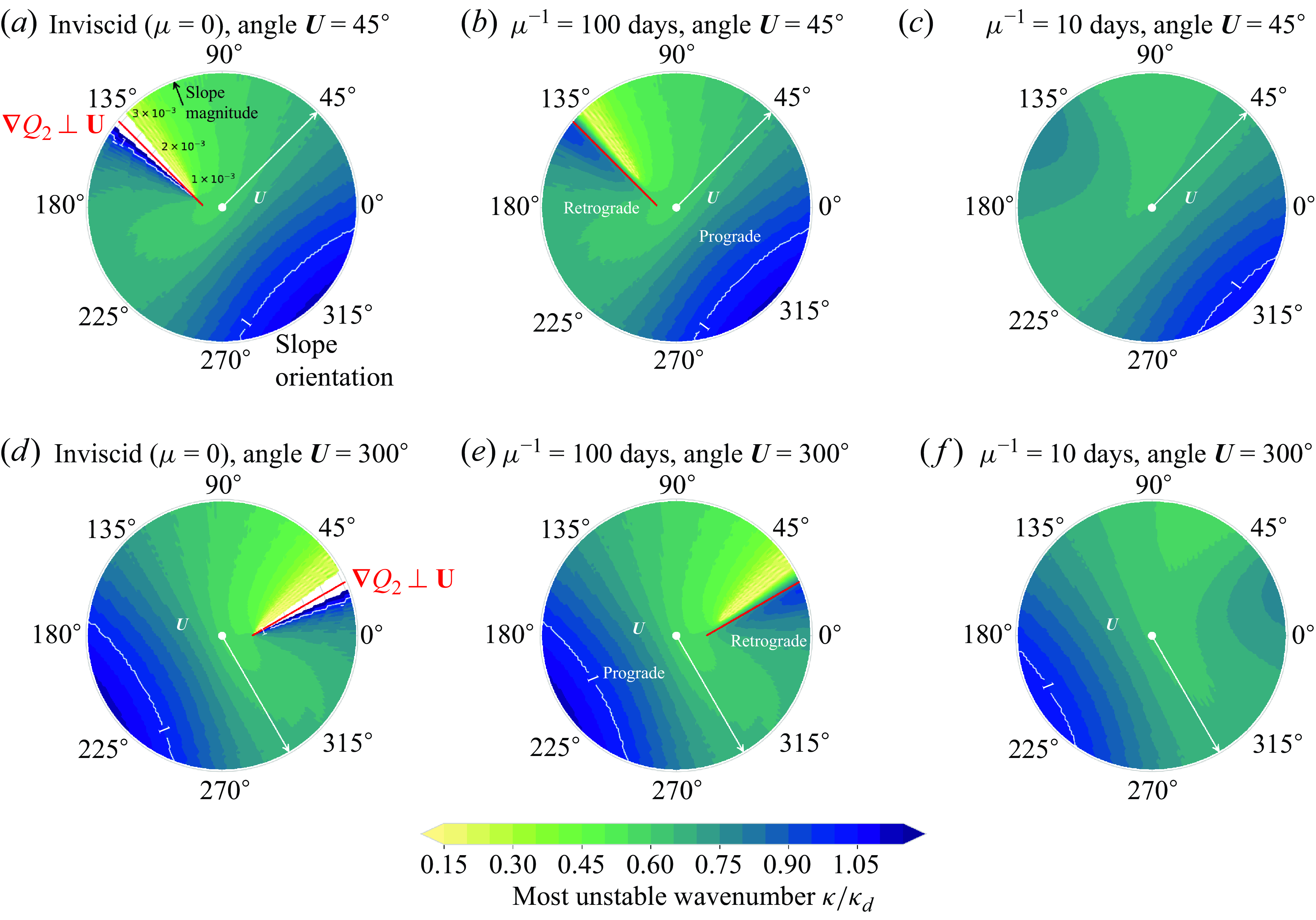
As figure 3 but showing the most unstable wavenumber. The $\kappa = \kappa _d$
contour is indicated in white.
$\kappa = \kappa _d$
contour is indicated in white.
As figure 3 but showing the propagation direction of the most unstable wave.
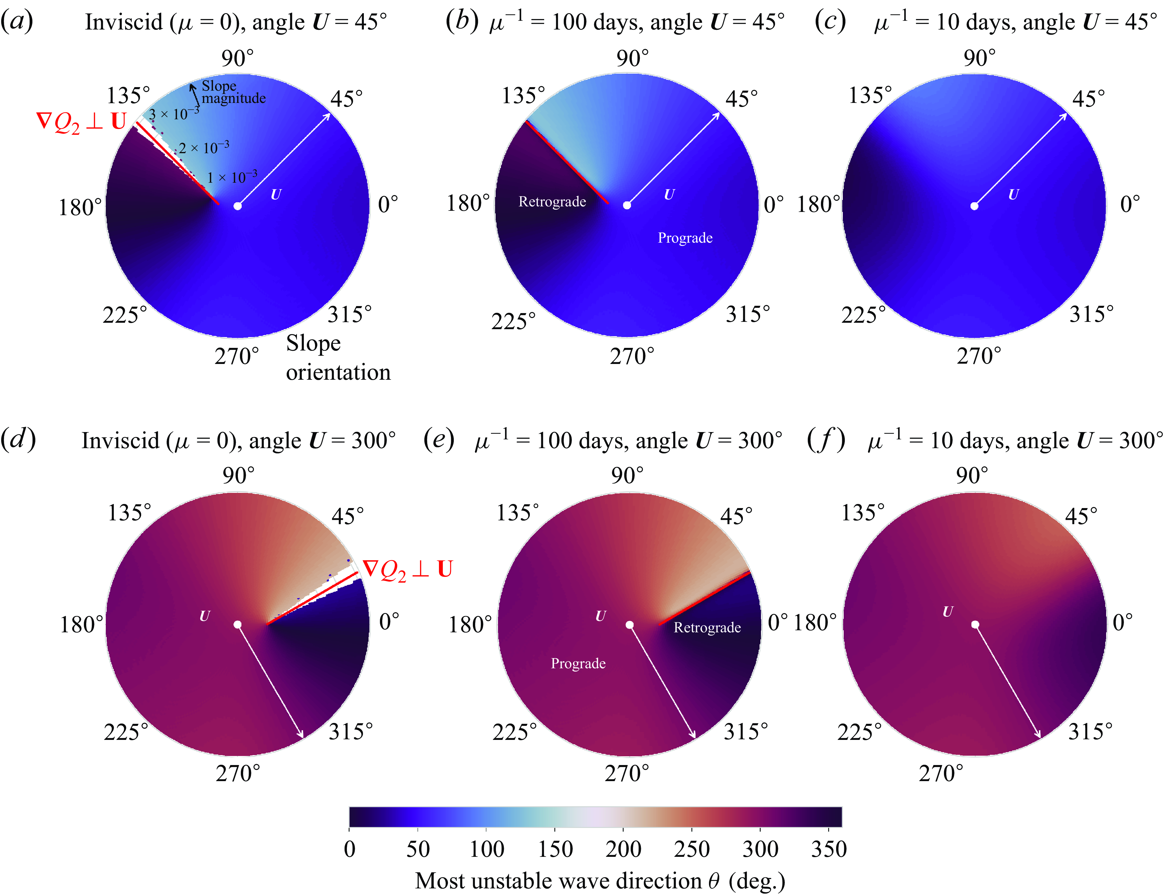
Figure 4 shows the most unstable wavenumber as a function of bottom slope orientation and magnitude. Generally, retrograde slopes favour lower wavenumbers (larger scales), whereas prograde slopes favour higher wavenumbers (smaller scales), as in Leng & Bai (Reference Leng and Bai2018). An interesting feature occurs around the line $\boldsymbol{\nabla} Q_2 \perp \boldsymbol{U}$
in the inviscid and weak friction cases: there is a discontinuity across this line with a switch from a low wavenumber mode to a high wavenumber mode. The discontinuity goes in opposite directions for the two shear orientations considered here; the shift from low to high wavenumber occurs in the anticlockwise direction for shear angle
$\boldsymbol{\nabla} Q_2 \perp \boldsymbol{U}$
in the inviscid and weak friction cases: there is a discontinuity across this line with a switch from a low wavenumber mode to a high wavenumber mode. The discontinuity goes in opposite directions for the two shear orientations considered here; the shift from low to high wavenumber occurs in the anticlockwise direction for shear angle $45^\circ$
, and in the clockwise direction for shear angle
$45^\circ$
, and in the clockwise direction for shear angle $300^\circ$
. Other shear orientations between
$300^\circ$
. Other shear orientations between $0^\circ$
and
$0^\circ$
and $270^\circ$
show the same behaviour as for
$270^\circ$
show the same behaviour as for $45^\circ$
, and other shear orientations between
$45^\circ$
, and other shear orientations between $270^\circ$
and
$270^\circ$
and $360^\circ$
show the same as for
$360^\circ$
show the same as for $300^\circ$
(not shown here). The discontinuity across
$300^\circ$
(not shown here). The discontinuity across $\boldsymbol{\nabla} Q_2 \perp \boldsymbol{U}$
is smoothed for strong friction, and the most unstable wavenumber becomes more uniform for all bottom slope magnitudes and orientations. However, the most unstable wavenumber remains asymmetric in the line
$\boldsymbol{\nabla} Q_2 \perp \boldsymbol{U}$
is smoothed for strong friction, and the most unstable wavenumber becomes more uniform for all bottom slope magnitudes and orientations. However, the most unstable wavenumber remains asymmetric in the line $\boldsymbol{\nabla} Q_2 \perp \boldsymbol{U}$
for retrograde slopes, as opposed to the maximum growth rate. Note that periodic patterns appear, most notably in the low wavenumber mode close to the line
$\boldsymbol{\nabla} Q_2 \perp \boldsymbol{U}$
for retrograde slopes, as opposed to the maximum growth rate. Note that periodic patterns appear, most notably in the low wavenumber mode close to the line $\boldsymbol{\nabla} Q_2 \perp \boldsymbol{U}$
. These are in part due to the resolution of the values of
$\boldsymbol{\nabla} Q_2 \perp \boldsymbol{U}$
. These are in part due to the resolution of the values of $\kappa$
and
$\kappa$
and $\theta$
that were tested, but some periodic signal still remains even for higher resolution (not shown here). This is likely due to interactions of higher harmonics. As the patterns appear within a regime where the growth rates are very weak, they are not of great importance for the qualitative behaviour of the instability as a function of slope.
$\theta$
that were tested, but some periodic signal still remains even for higher resolution (not shown here). This is likely due to interactions of higher harmonics. As the patterns appear within a regime where the growth rates are very weak, they are not of great importance for the qualitative behaviour of the instability as a function of slope.
Finally, figure 5 shows the propagation direction of the most unstable wave as a function of the bottom slope. If the phase speed (real part of $c$
) of the most unstable wave is positive, then the propagation direction is given by the orientation
$c$
) of the most unstable wave is positive, then the propagation direction is given by the orientation $\theta$
of the most unstable wavenumber vector; if the phase speed is negative, then the propagation direction is exactly opposite to
$\theta$
of the most unstable wavenumber vector; if the phase speed is negative, then the propagation direction is exactly opposite to $\theta$
(shift of
$\theta$
(shift of $180^\circ$
). For the inviscid and weak friction cases, again there is a clear asymmetry between prograde and retrograde slopes. For prograde slopes, the propagation direction is close to the direction of the mean shear. For retrograde slopes, on the other hand, the most unstable wave crosses the mean flow, until the propagation direction is close to the normal direction of the mean shear around the line
$180^\circ$
). For the inviscid and weak friction cases, again there is a clear asymmetry between prograde and retrograde slopes. For prograde slopes, the propagation direction is close to the direction of the mean shear. For retrograde slopes, on the other hand, the most unstable wave crosses the mean flow, until the propagation direction is close to the normal direction of the mean shear around the line $\boldsymbol{\nabla} Q_2 \perp \boldsymbol{U}$
. This is in agreement with the case studies considered by Leng & Bai (Reference Leng and Bai2018). As in figure 4, a discontinuity occurs across
$\boldsymbol{\nabla} Q_2 \perp \boldsymbol{U}$
. This is in agreement with the case studies considered by Leng & Bai (Reference Leng and Bai2018). As in figure 4, a discontinuity occurs across $\boldsymbol{\nabla} Q_2 \perp \boldsymbol{U}$
: the propagation direction switches by
$\boldsymbol{\nabla} Q_2 \perp \boldsymbol{U}$
: the propagation direction switches by $180^\circ$
across this line. This switch ensures that the most unstable wave always propagates at an acute angle to the mean shear. Over a retrograde slope with
$180^\circ$
across this line. This switch ensures that the most unstable wave always propagates at an acute angle to the mean shear. Over a retrograde slope with $\boldsymbol{\nabla} Q_2 \boldsymbol{\cdot} \boldsymbol{U} \gt 0$
, the most unstable wave travels upslope, with the mean shear to its right; if
$\boldsymbol{\nabla} Q_2 \boldsymbol{\cdot} \boldsymbol{U} \gt 0$
, the most unstable wave travels upslope, with the mean shear to its right; if $\boldsymbol{\nabla} Q_2 \boldsymbol{\cdot} \boldsymbol{U} \lt 0$
, then it travels downslope with
$\boldsymbol{\nabla} Q_2 \boldsymbol{\cdot} \boldsymbol{U} \lt 0$
, then it travels downslope with $\boldsymbol{U}$
to its left. For strong friction, the discontinuity across
$\boldsymbol{U}$
to its left. For strong friction, the discontinuity across $\boldsymbol{\nabla} Q_2 \perp \boldsymbol{U}$
disappears, as does the prograde–retrograde asymmetry: the waves all travel parallel to the mean shear.
$\boldsymbol{\nabla} Q_2 \perp \boldsymbol{U}$
disappears, as does the prograde–retrograde asymmetry: the waves all travel parallel to the mean shear.
4. Conclusions and discussion
We have used the two-layer QG model to study the joint effect of a planetary PV gradient, topographic PV gradients of varying orientation and magnitude, and bottom friction on baroclinic instability. A well-known instability condition of the inviscid two-layer model with a zonal mean shear and a linear meridional bottom slope is that the PV gradient must change sign between the two layers, and as a result there is a critical retrograde slope beyond which all instability is suppressed. We generalised this condition to account for other orientations of the mean shear and the bottom slope. A flow can be stable for all wavenumbers only for very specific slopes. Moreover, the instability condition no longer holds if bottom friction is present.
We first derived the instability condition with bottom friction (3.14). The system is unstable for wavenumber vectors with wave angle $\theta$
as long as the component of the shear parallel to the wavenumber vector is sufficiently strong; the critical shear for instability is independent of both the friction coefficient and the bottom slope. Bottom friction destabilises the system for all slope orientations and magnitudes, in line with previous studies (e.g. Holopainen Reference Holopainen1961; Swaters Reference Swaters2009; Lee Reference Lee2010a
; Willcocks & Esler Reference Willcocks and Esler2012). The instability condition (3.14) shows that even systems with all-positive or all-negative PV gradients can be unstable. With weak friction, the maximum growth rate is still much weaker for retrograde than for prograde slopes; as friction increases, this asymmetry disappears, and all growth rates become weaker. With strong friction, the growth rates are very weak. Hence even though friction destabilises otherwise fully stable modes, it also suppresses the growth of the unstable modes.
$\theta$
as long as the component of the shear parallel to the wavenumber vector is sufficiently strong; the critical shear for instability is independent of both the friction coefficient and the bottom slope. Bottom friction destabilises the system for all slope orientations and magnitudes, in line with previous studies (e.g. Holopainen Reference Holopainen1961; Swaters Reference Swaters2009; Lee Reference Lee2010a
; Willcocks & Esler Reference Willcocks and Esler2012). The instability condition (3.14) shows that even systems with all-positive or all-negative PV gradients can be unstable. With weak friction, the maximum growth rate is still much weaker for retrograde than for prograde slopes; as friction increases, this asymmetry disappears, and all growth rates become weaker. With strong friction, the growth rates are very weak. Hence even though friction destabilises otherwise fully stable modes, it also suppresses the growth of the unstable modes.
We examined how the growth rates vary with the orientation of the mean shear $\boldsymbol{U}$
and the bottom slope. This is similar to Leng & Bai (Reference Leng and Bai2018), but they considered only configurations in which the bottom slope is perpendicular to the mean shear. We considered two different orientations of
$\boldsymbol{U}$
and the bottom slope. This is similar to Leng & Bai (Reference Leng and Bai2018), but they considered only configurations in which the bottom slope is perpendicular to the mean shear. We considered two different orientations of $\boldsymbol{U}$
, and studied all possible orientations of the bottom slope. The system can be stable only if there is no bottom friction and the lower layer PV gradient is perpendicular to the mean shear. The slope for which this criterion holds is retrograde; prograde slopes are always unstable, and have higher growth rates. This generalises earlier findings that a system that is stable with a zonal shear and zonal isobaths can be destabilised by even a weakly non-zonal shear or weakly zonal slope (e.g. Kamenkovich & Pedlosky Reference Kamenkovich and Pedlosky1996; Chen & Kamenkovich Reference Chen and Kamenkovich2013). Friction destabilises the system for all slope orientations and magnitudes, but also suppresses the growth rates. The dependency of the growth rate on the slope disappears with increasing friction. Furthermore, we found that with no or weak friction, the most unstable wave propagates along the mean flow for prograde slopes but crosses the mean flow for retrograde slopes. This agrees with the findings from Leng & Bai (Reference Leng and Bai2018). An interesting new finding is that there is a discontinuity in the wavenumber and propagation direction of the most unstable wave around slope vectors for which
$\boldsymbol{U}$
, and studied all possible orientations of the bottom slope. The system can be stable only if there is no bottom friction and the lower layer PV gradient is perpendicular to the mean shear. The slope for which this criterion holds is retrograde; prograde slopes are always unstable, and have higher growth rates. This generalises earlier findings that a system that is stable with a zonal shear and zonal isobaths can be destabilised by even a weakly non-zonal shear or weakly zonal slope (e.g. Kamenkovich & Pedlosky Reference Kamenkovich and Pedlosky1996; Chen & Kamenkovich Reference Chen and Kamenkovich2013). Friction destabilises the system for all slope orientations and magnitudes, but also suppresses the growth rates. The dependency of the growth rate on the slope disappears with increasing friction. Furthermore, we found that with no or weak friction, the most unstable wave propagates along the mean flow for prograde slopes but crosses the mean flow for retrograde slopes. This agrees with the findings from Leng & Bai (Reference Leng and Bai2018). An interesting new finding is that there is a discontinuity in the wavenumber and propagation direction of the most unstable wave around slope vectors for which $\boldsymbol{\nabla} Q_2 \perp \boldsymbol{U}$
. Very small changes in the slope orientation can result in large changes in the instability scale and a
$\boldsymbol{\nabla} Q_2 \perp \boldsymbol{U}$
. Very small changes in the slope orientation can result in large changes in the instability scale and a $180^\circ$
shift in the propagation direction of the most unstable mode, from parallel to anti-parallel to the slope. For strong friction, the most unstable wave always travels along the mean flow.
$180^\circ$
shift in the propagation direction of the most unstable mode, from parallel to anti-parallel to the slope. For strong friction, the most unstable wave always travels along the mean flow.
A limitation of the two-layer QG model is that it does not account for interior PV gradients. The two layers are dynamically linked, hence the bottom friction and bottom slope affect both layers. In contrast, Lobo et al. (Reference Lobo, Griffies and Zhang2025) showed that while prograde flows in a three-layer QG model are reasonably represented by the two-layer model, retrograde flows are not. The reason is that retrograde flows can support surface-intensified instabilities that are almost insensitive to bottom topography, causing the flow to be more unstable than with two layers. The addition of interior PV gradients associated with an extra layer or continuous stratification might thus affect the instability conditions. An interesting case for further research would be the effect of bottom friction and misalignment of PV gradients on baroclinic instability in the three-layer QG model.
Also of interest is the impact of the type of friction on stability. The present study considers only bottom friction, but not lateral eddy friction. Moreover, we considered only linear (Ekman) friction, but many models use quadratic bottom friction instead (e.g. Chang & Held Reference Chang and Held2021; Chen Reference Chen2023; Deng & Wang Reference Deng and Wang2024). Linear and quadratic bottom friction have different impacts on the turbulence properties of the two-layer model (Grianik et al. Reference Grianik, Held, Smith and Vallis2004; Gallet & Ferrari Reference Gallet and Ferrari2020, Reference Gallet and Ferrari2021) and may thus affect stability in distinct ways, possibly in terms of frictional instability. As linear stability analysis is no longer possible with quadratic friction, such analysis would necessarily be numerical.
Though highly idealised, the present findings could help to improve understanding of baroclinic instability in the ocean. They shed light on the dependency of instability characteristics on the bottom slope and bottom friction, and demonstrate that with increasing friction, the system transitions from slope-dominated to friction-dominated. This could be important for understanding the nonlinear dynamics as well (Berloff & Kamenkovich Reference Berloff and Kamenkovich2013a ,Reference Berloff and Kamenkovich b ). For example, it would be interesting to know how the energy levels of mesoscale eddies depend on the bottom slope and bottom friction, and if they show a transition from slope-dominated to friction-dominated. Unfortunately, little is known on the strength and spatial variability of the bottom friction in the ocean, and estimates can differ by up to two orders of magnitude (Arbic & Flierl Reference Arbic and Flierl2004a ). More data on the frictional strength distribution in the global ocean are needed to properly understand which mechanism is dominant in setting the instability characteristics in the ocean. Stability caused by steep retrograde bottom slopes holds only in a very specific case: in the absence of bottom friction, when the planetary, topographic and stretching PV gradients are all aligned. Since such a specific alignment of the PV gradients is extremely rare and the seafloor is not frictionless, stabilisation by steep slopes probably does not occur in the ocean. Likewise, the ‘classical’ two-layer model with its zonal mean shear, meridional bottom slope and no friction might not be so relevant in practice when studying baroclinic instability in the ocean.
Acknowledgements
We thank M. Lobo for insightful discussions, and four anonymous reviewers for their helpful feedback on the manuscript.
Funding
M.F.S. and S.G. were funded by the UU-NIOZ project ‘The intermittency of large-scale ocean mixing’ (project no. NZ4543.3). A.P. was supported with Institutional Funding at the National Oceanography Centre, UK. M.L.J.B. was funded by the programme of the Netherlands Earth System Science Centre (NESSC), financially supported by the Ministry of Education, Culture and Science (OCW, grant no. 024.002.001). J.H.L. was supported by the Research Council of Norway (RCN) project ‘The Rough Ocean’ (project no. 302743). P.E.I. was funded by the RCN project TopArctic (project no. 314826).
Declaration of interests
The authors report no conflict of interest.
Data availability statement
The code used to create the figures in this study is available at https://github.com/MiriamSterl/TwoLayerLSA.
Author contributions
M.F.S.: conceptualisation, formal analysis, methodology, visualisation, writing – original draft. A.P.: conceptualisation, writing – review and editing. S.G.: funding acquisition, supervision, writing – review and editing. M.L.J.B.: funding acquisition, supervision, writing – review and editing. J.H.L.: conceptualisation, writing – review and editing. P.E.I.: writing – review and editing.


 Open access