


1. Introduction
Shallow cumulus convection is a common form of moist convection that reaches a few kilometres above the convective mixed layer and dissipates without producing significant precipitation (e.g. Malkus Reference Malkus1954; Emanuel Reference Emanuel1994; Zuidema et al. Reference Zuidema, Li, Hill, Bariteau, Rilling, Fairall, Brewer, Albrecht and Hare2012). A shallow cumulus usually consists of localised buoyant air elements called ‘thermal bubbles’ (Scorer & Ludlam Reference Scorer and Ludlam1953; Yano Reference Yano2014), which arise from convective structures in the mixed layer (Stull Reference Stull1985). Water vapour condenses and releases latent heat as the ascending thermal bubble cools by adiabatic expansion, providing additional buoyancy, thus lifting it into the stably stratified troposphere (e.g. Wallace & Hobbs Reference Wallace and Hobbs2006). While ascending, the thermal bubble entrains dry air, mixes with the liquid droplets, and causes evaporative cooling (Stommel Reference Stommel1947; Paluch Reference Paluch1979; de Rooy et al. Reference de Rooy, Bechtold, Fröhlich, Hohenegger, Jonker, Mironov, Pier Siebesma, Teixeira and Yano2013). This evaporative cooling drives a downdraft surrounding the cloud (Blyth et al. Reference Blyth, Cooper and Jensen1988; Heus & Jonker Reference Heus and Jonker2008), which dries and cools the boundary layer through direct transport and turbulent mixing (Emanuel Reference Emanuel1989; Thayer-Calder & Randall Reference Thayer-Calder and Randall2015; de Szoeke Reference de Szoeke2018).
Modelling the effects of these small-scale shallow cumuli is crucial for parametrizing the vertical transport of tracers and momentum in the lower troposphere (Bretherton et al. Reference Bretherton, McCaa and Grenier2004). Higher humidity in the boundary layer fosters cumulus clouds. Thus the cloud may be seen as a ‘valve’ that releases the humidity accumulated by surface evaporation. However, shallow cumuli are not the only modulators of boundary layer humidity; convective cells in the boundary layer also entrain dry air from above (e.g. Lilly Reference Lilly1968; Deardorff et al. Reference Deardorff1970; de Szoeke Reference de Szoeke2018). The relative contribution of cumulus versus boundary layer cells in mixing the lower troposphere remains an open question (Thayer-Calder & Randall Reference Thayer-Calder and Randall2015).
This paper introduces a novel laboratory experiment to make modelling progress on this question, focusing on mixing by shallow cumulus convection. While observations and numerical simulations have been the main tools for studying clouds, laboratory experiments can provide a unique complementary perspective (e.g. Bohren Reference Bohren2013; Yano Reference Yano2014; Shaw et al. Reference Shaw2020). The main challenge is mimicking the water phase change in the laboratory, which includes the condensation heating that drives the updraft, and the evaporative cooling that drives the downdraft. Faithfully representing condensation heating would require a 1 km tall apparatus. To study cloud dynamics in the laboratory, analogies must therefore be found, with the awareness that no analogy is complete. Previous experiments simulated condensation-driven updrafts and evaporation-driven downdrafts separately. The updraft has been simulated with the heat released from a chemical reaction (Hadlock & Hess Reference Hadlock and Hess1968), gas bubbles (Turner Reference Turner1963; Turner & Lilly Reference Turner and Lilly1963), the selective radiative absorption of chemicals (Krishnamurti Reference Krishnamurti1998), a heating coil (Narasimha et al. Reference Narasimha, Diwan, Duvvuri, Sreenivas and Bhat2011), the radiation from a lamp (Zhao et al. Reference Zhao, Xiong, Hu and Zhu2001), and so on. The downdraft has been simulated with the release of saltwater or heavy particles into fresh water (Simpson & Britter Reference Simpson and Britter1980; Yao & Lundgren Reference Yao and Lundgren1996; Kriaa et al. Reference Kriaa, Subra, Favier and Le Bars2022). These methods are less suited to simulating shallow cumuli, which involves the interaction between boundary layer cells, cumulus updrafts and downdrafts.
To simulate shallow cumuli, we will rely on boiling, a vaporisation process that occurs when the water temperature exceeds the boiling point. Boiling is a threshold-dependent phenomenon that limits the water temperature around the boiling point by absorbing the heat of vaporisation and mixing the superheated water with the colder water above (Collier & Thome Reference Collier and Thome1994; Oresta et al. Reference Oresta, Verzicco, Lohse and Prosperetti2009). Buoyancy is gained from the volume expansion during vaporisation, and lost from the subsequent condensation. Such a transient buoyancy gain and loss appear promising to simulate the updrafts and downdrafts in shallow cumuli. To improve the analogy, we must also reproduce the mostly stable stratification in the atmosphere, which traps moisture in the boundary layer, thus facilitating its accumulation. This is the idea behind our boiling stratified flow experiment, essentially coupling boiling with two-layer Rayleigh–Bénard convection (Turner Reference Turner1965; Davaille Reference Davaille1999). Although some studies have investigated the boiling of two layers of immiscible fluids such as water and oil (e.g. Mori Reference Mori1978, Reference Mori1985; Greene et al. Reference Greene, Chen and Conlin1988; Takahashi et al. Reference Takahashi, Tasaka, Murai, Takeda and Yanagisawa2010; Filipczak et al. Reference Filipczak, Troniewski and Witczak2011; Onishi et al. Reference Onishi, Ohta, Ohtani, Fukuyama and Kobayashi2013; Kawanami et al. Reference Kawanami, Matsuhiro, Hara, Honda and Takagaki2020), the boiling of two separate layers of miscible fluids appears to receive little attention.
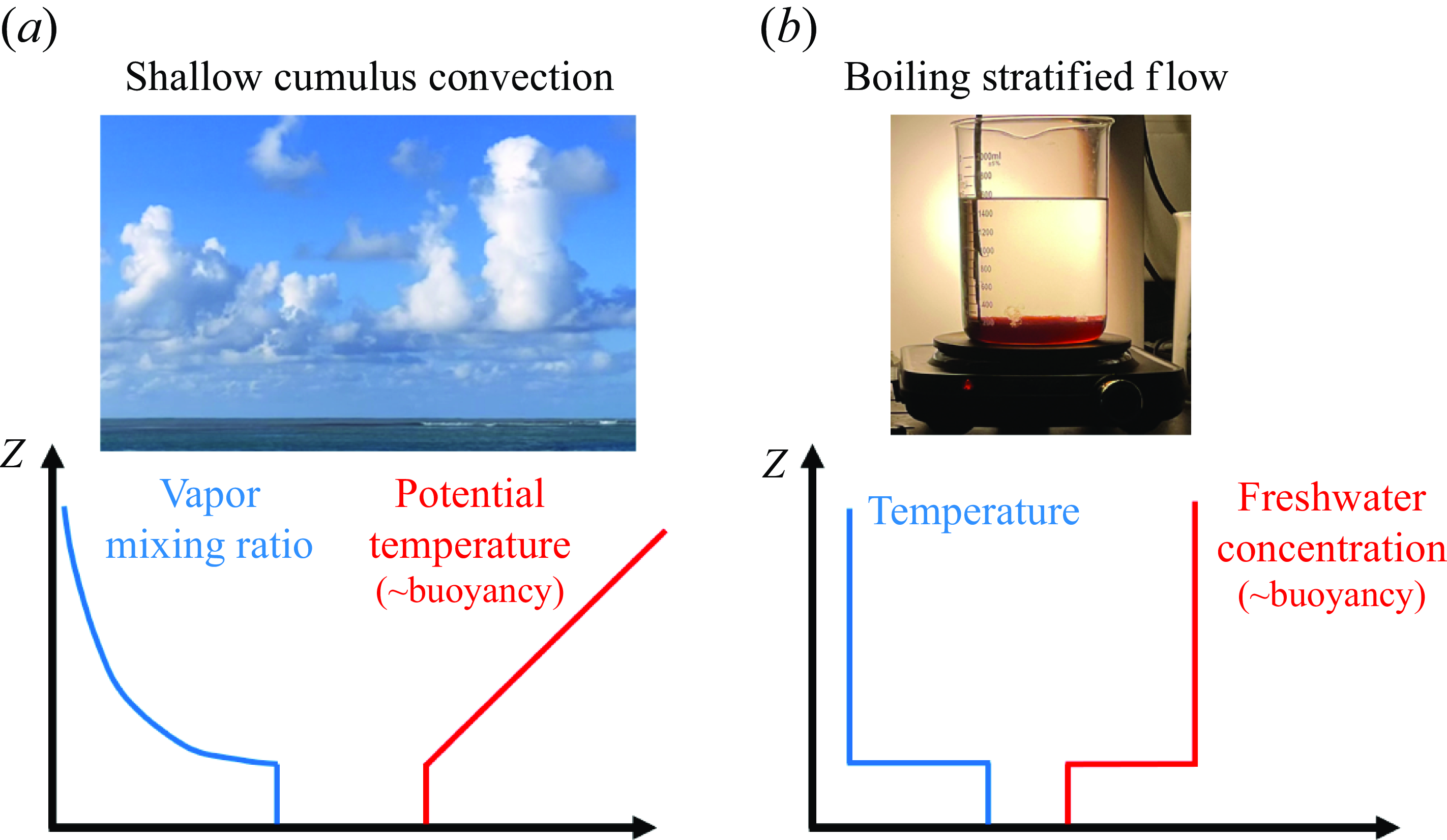
Our boiling stratified flow is set up with a freshwater layer mimicking the free troposphere above a thin layer of syrup mimicking the atmospheric boundary layer (figure 1). The water temperature is analogous to the atmospheric water vapour mixing ratio. The vapour plays a relatively minor role in the air buoyancy, but a sufficiently humid boundary layer is necessary to initiate cumulus convection. The freshwater concentration is analogous to the atmospheric potential temperature controlling buoyancy. We will show that boiling produces vapour bubbles that propel the surrounding syrup into vortex rings (a ‘flow with circular vortex lines’ according to Batchelor Reference Batchelor1967). Although bubbles quench quickly upon formation, the vortex rings carry the syrup to travel a much longer distance, stir the syrup–water interface, and entrain and mix cold water into the syrup layer. This process competes with convective cells in the syrup layer for transferring heat. We argue that this competition is analogous to that between shallow cumuli and boundary layer cells for transporting water vapour in the troposphere.
The paper is organised as follows. Section 2 introduces the experimental set-up. Section 3 analyses the flow evolution of a reference experiment, which inspires the theory in § 4. Section 5 applies and verifies the theory to understand experiments across the parameter space. Section 6 extends the theory to study the transition between two types of boiling (transient and steady). Section 7 summarises the fluid dynamics findings and assesses the analogy with the atmosphere.
(a) Shallow cumulus convection and idealised profiles of the water vapour mixing ratio and potential temperature, and (b) the experimental set-up, and the corresponding idealised profiles of temperature and freshwater concentration. The buoyancy profile is dominated by the red line, i.e. the potential temperature in the atmosphere and freshwater concentration in most of our experiments.
2. The boiling stratified flow experiment
2.1. Experimental set-up
The experimental set-up is shown in figure 1. It consists of a 2000 ml beaker with diameter approximately 130 mm. The beaker is filled with a layer of dark corn syrup water solution underlying a thicker layer of tap fresh water. Here, $\rho _{s,max}\approx 1.4\times 10^3$
kg m
$\rho _{s,max}\approx 1.4\times 10^3$
kg m $^{-3}$
is the density of the pure syrup, and
$^{-3}$
is the density of the pure syrup, and $\rho _w \approx 1\times 10^3$
kg m
$\rho _w \approx 1\times 10^3$
kg m $^{-3}$
is the density of the fresh water. The beaker is heated on an electric hot plate with adjustable heating power. More details on the set-up are given in Appendix A.1. When diluted, the density of the syrup solution
$^{-3}$
is the density of the fresh water. The beaker is heated on an electric hot plate with adjustable heating power. More details on the set-up are given in Appendix A.1. When diluted, the density of the syrup solution $\rho _s$
obeys
$\rho _s$
obeys
 \begin{eqnarray} \rho _s = S \rho _{s,max} + ( 1 - S ) \rho _w, \quad \end{eqnarray}
where $0\leqslant S\leqslant 1$
is the dimensionless syrup concentration:
$0\leqslant S\leqslant 1$
is the dimensionless syrup concentration:
 \begin{eqnarray} S \equiv \frac {\rho _s-\rho _w}{\rho _{s,max}-\rho _w}. \end{eqnarray}
The system is required to be statically stable at the onset of boiling. The vertical gradient of syrup concentration stabilises the two-layer configuration against the destabilizing effect of the temperature gradient. The buoyancy $b$
(in m s
$b$
(in m s $^{-2}$
) is defined as
$^{-2}$
) is defined as
 \begin{eqnarray} b = g \left ( -\gamma _s S + \gamma _T T \right ), \end{eqnarray}
where $g=9.8$
m s
$g=9.8$
m s $^{-2}$
is the gravitational acceleration,
$^{-2}$
is the gravitational acceleration, $\gamma _s \equiv (\rho _{s,max}-\rho _w)/\rho _w=0.4$
is the syrup concentration coefficient, and
$\gamma _s \equiv (\rho _{s,max}-\rho _w)/\rho _w=0.4$
is the syrup concentration coefficient, and $\gamma _T\approx 6\times 10^{-4}$
K
$\gamma _T\approx 6\times 10^{-4}$
K $^{-1}$
is the volumetric thermal expansion coefficient of the solution, taken as the value for 80
$^{-1}$
is the volumetric thermal expansion coefficient of the solution, taken as the value for 80 $^\circ$
C pure water (The Engineering ToolBox 2003). At the onset of boiling, the water layer temperature is
$^\circ$
C pure water (The Engineering ToolBox 2003). At the onset of boiling, the water layer temperature is $T_w \approx 30\,^\circ$
C (slightly above the 20
$T_w \approx 30\,^\circ$
C (slightly above the 20 $^\circ$
C room temperature), while the syrup layer is at the boiling temperature
$^\circ$
C room temperature), while the syrup layer is at the boiling temperature $T_* \approx 100\,^\circ$
C. We let the characteristic temperature difference be
$T_* \approx 100\,^\circ$
C. We let the characteristic temperature difference be $T_*-T_w = (100-30)\,^\circ \textrm{C}=70\,^\circ \textrm{C}$
. To make the system stable,
$T_*-T_w = (100-30)\,^\circ \textrm{C}=70\,^\circ \textrm{C}$
. To make the system stable, $S$
must be above a minimum value
$S$
must be above a minimum value $S_{min}$
:
$S_{min}$
:
 \begin{eqnarray} S_{min} \equiv \frac {\gamma _T \left ( T_*-T_w \right )}{\gamma _s} \approx 0.11. \end{eqnarray}
Since the initial concentration obeys $S_0 \gg S_{min}$
in most of our experiments, the buoyancy from the syrup is dominant. The freshwater concentration
$S_0 \gg S_{min}$
in most of our experiments, the buoyancy from the syrup is dominant. The freshwater concentration $(1-S)$
is analogous to the potential temperature in the atmosphere, and both increase with height. They produce a stable background buoyancy stratification. The temperature
$(1-S)$
is analogous to the potential temperature in the atmosphere, and both increase with height. They produce a stable background buoyancy stratification. The temperature $T$
in the experiment is analogous to the water vapour mixing ratio in the atmosphere, and both decrease with height. They represent the potential for gaining extra buoyancy from boiling and condensation heating. In the experiment, the heat is transported by convective cells in the beaker, the water phase change, and the bubble-induced fluid motion.
$T$
in the experiment is analogous to the water vapour mixing ratio in the atmosphere, and both decrease with height. They represent the potential for gaining extra buoyancy from boiling and condensation heating. In the experiment, the heat is transported by convective cells in the beaker, the water phase change, and the bubble-induced fluid motion.
We use syrup because it has higher density and viscosity than water, both of which suppress interfacial heat and mass transfer (Turner Reference Turner1986). The high syrup viscosity is crucial in that it enables the lower layer to reach the boiling point before the two-layer stratification is eroded by turbulence. The high viscosity does not have a direct analogy to the atmosphere, but it might be thought of as an amplifier of the density stratification effect.
The flow is recorded with a camera from a side view, providing an integrated view of the syrup concentration. Temperature is measured with thermocouples located at $z=1$
, 3, 5 and 7 cm above the bottom of the beaker, though this paper discusses only the
$z=1$
, 3, 5 and 7 cm above the bottom of the beaker, though this paper discusses only the $z=1$
and 5 cm data.
$z=1$
and 5 cm data.
2.2. List of experiments
Several parameters govern the system:
-
(i) the surface heating flux $F_s$
, which is analogous to the heating of the lower atmosphere from Earth’s surface and by radiation
$F_s$
, which is analogous to the heating of the lower atmosphere from Earth’s surface and by radiation -
(ii) the initial syrup layer thickness
$h_0$
, which is analogous to the thickness of the atmospheric convective boundary layer -
(iii) the initial syrup concentration
$S_0$
, which is analogous to the strength of buoyancy stratification near the top of the boundary layer -
(iv) the initial water layer thickness, which is analogous to the tropospheric depth.


We decided to leave the investigation of the effects of the water layer thickness for future work by keeping the initial freshwater thickness fixed to approximately 10 cm (corresponding to the 1400 ml scale on the beaker), much thicker than the convective penetration height.
We performed four groups of experiments, varying $F_s$
(F1–F5),
$F_s$
(F1–F5), $h_0$
(T1–T7),
$h_0$
(T1–T7), $S_0$
(S1–S7), and
$S_0$
(S1–S7), and $S_0$
and
$S_0$
and $h_0$
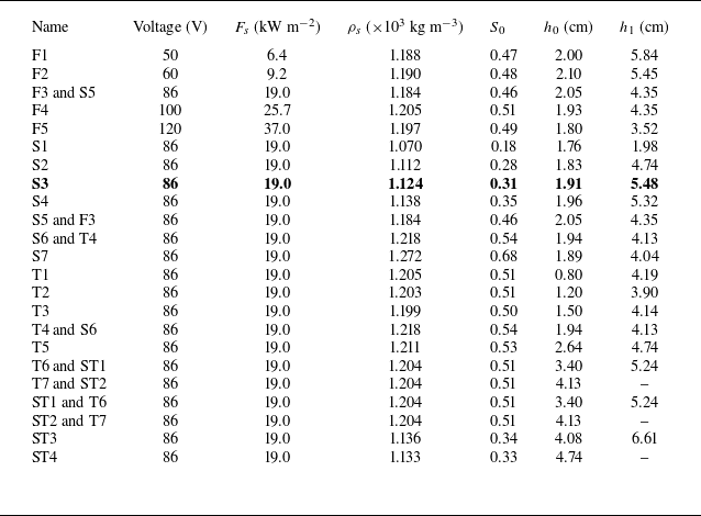
together (ST1–ST4), as shown in table 1. Note that the pairs of labels (F3, S5), (T4, S6), (T6, ST1) and (T7, ST2) correspond to the same experiments. Experiment S3 (in bold) is the reference experiment that will be analysed in detail.
$h_0$
together (ST1–ST4), as shown in table 1. Note that the pairs of labels (F3, S5), (T4, S6), (T6, ST1) and (T7, ST2) correspond to the same experiments. Experiment S3 (in bold) is the reference experiment that will be analysed in detail.
Table of experimental parameters, which include heating voltage, surface heat flux $F_s$
, initial syrup density
$F_s$
, initial syrup density $\rho _s$
, initial syrup concentration
$\rho _s$
, initial syrup concentration $S_0$
, and initial syrup thickness
$S_0$
, and initial syrup thickness $h_0$
. The post-boiling syrup thickness
$h_0$
. The post-boiling syrup thickness $h_1$
is shown in the rightmost column (the diagnostic procedure is detailed in § A.2). For experiments in the steady boiling regime (§ 5.3), their
$h_1$
is shown in the rightmost column (the diagnostic procedure is detailed in § A.2). For experiments in the steady boiling regime (§ 5.3), their $h_1$
is denoted as a dash. Note that some experiments are shared by different groups. Bold indicates S3, the reference experiment.
$h_1$
is denoted as a dash. Note that some experiments are shared by different groups. Bold indicates S3, the reference experiment.
We measured $S_0$
with a density meter, and
$S_0$
with a density meter, and $h_0$
with the video (using a pixel-to-length calibration). Note that the values of
$h_0$
with the video (using a pixel-to-length calibration). Note that the values of $S_0$
and
$S_0$
and $h_0$
reported in table 1 within an experimental group (e.g.
$h_0$
reported in table 1 within an experimental group (e.g. $S_0=0.47$
, 0.48, 0.46, etc. for the F group) are not exactly equal due to small fluctuations introduced in preparing the two layers.
$S_0=0.47$
, 0.48, 0.46, etc. for the F group) are not exactly equal due to small fluctuations introduced in preparing the two layers.
3. Basic physics and temporal evolution
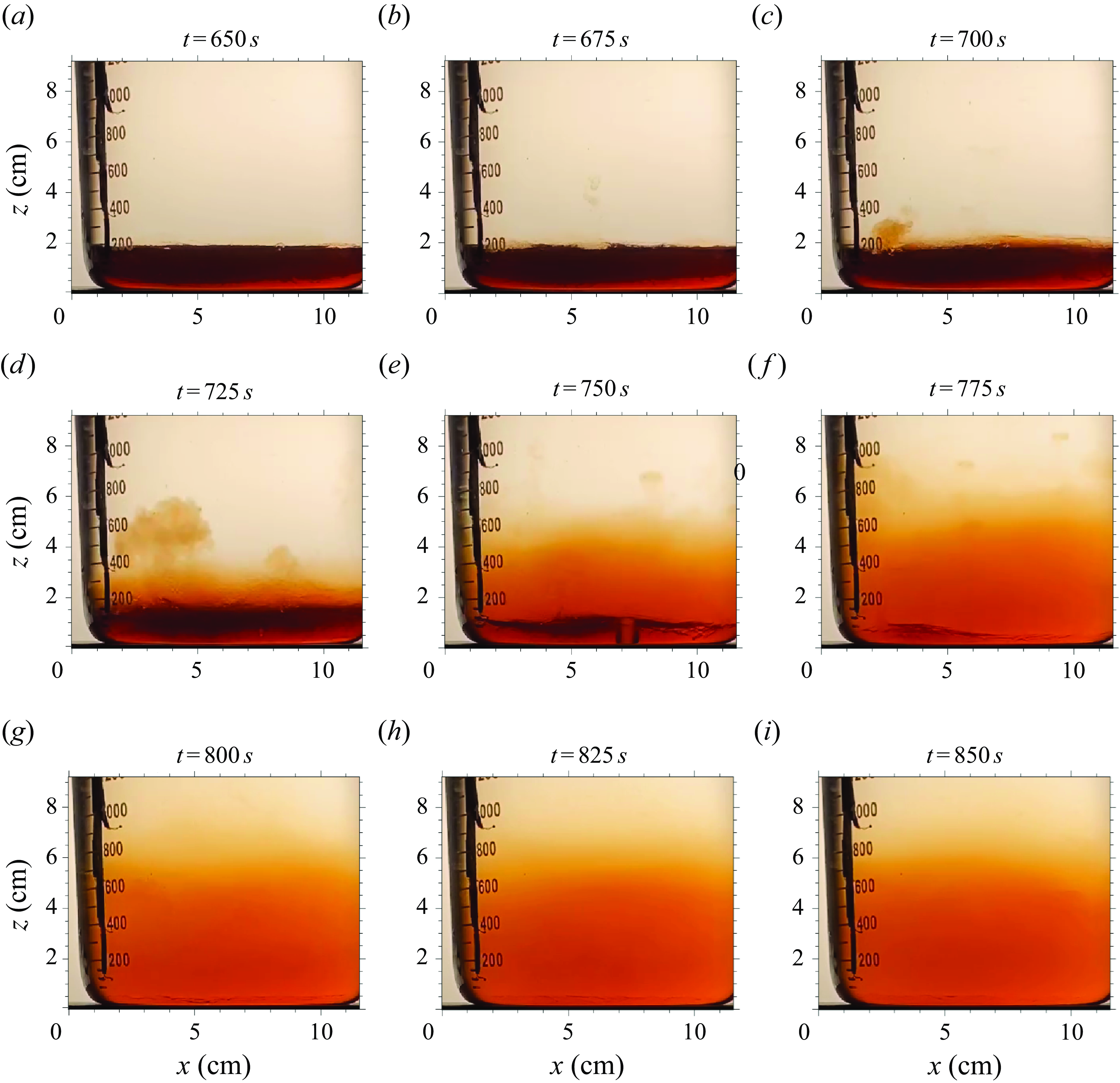
Figures 2 and 3 illustrate the basic physics of the boiling stratified flow in the reference experiment S3. We highlight three stages: the initial two-layer stage (visualised in figure 2 a–c), the boiling stage (figure 2 d–f), and the post-boiling two-layer stage (figure 2 g–i).
Reference experiment (S3): images at $t=650$
, 675, 700, 725, 750, 775, 800, 825 and 850 s showing (a–c) the initial two-layer stage, (d–f) the boiling stage, and (g–i) the post-boiling two-layer stage. The black columnar object near the beaker’s scale is the thermocouple array. A supplementary movie is available at https://doi.org/10.5281/zenodo.11222908.
$t=650$
, 675, 700, 725, 750, 775, 800, 825 and 850 s showing (a–c) the initial two-layer stage, (d–f) the boiling stage, and (g–i) the post-boiling two-layer stage. The black columnar object near the beaker’s scale is the thermocouple array. A supplementary movie is available at https://doi.org/10.5281/zenodo.11222908.
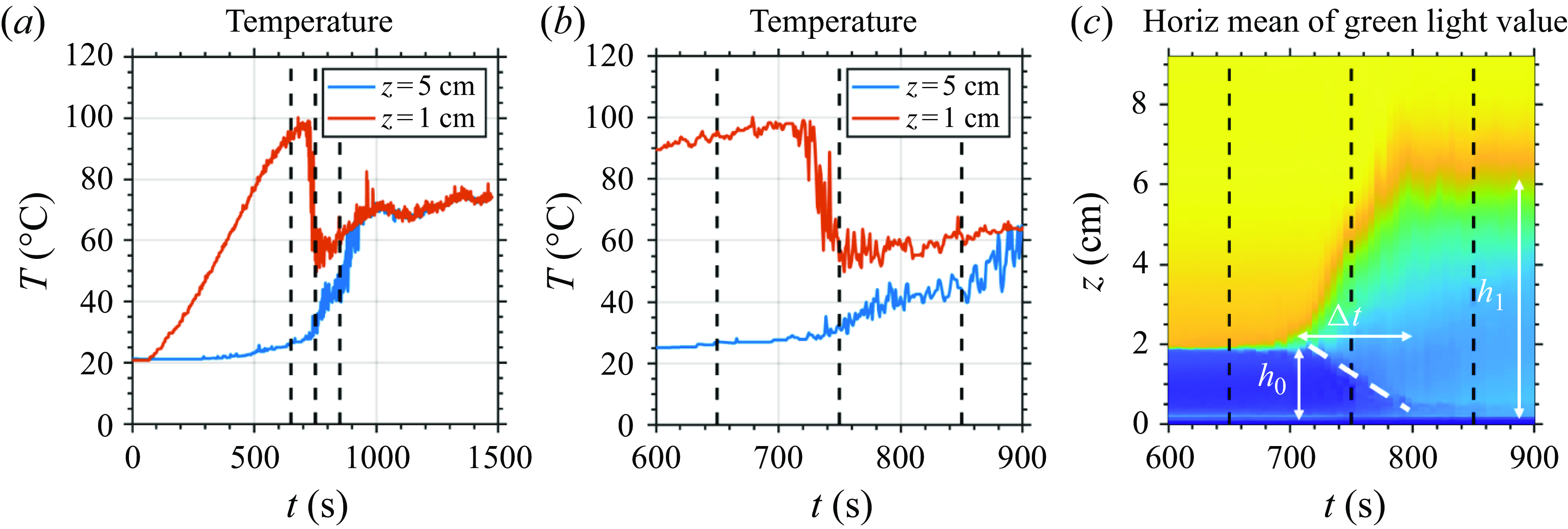
Quantitative measurements of the reference experiment S3. (a) The temperature time series at $z=5$
cm (blue line) and
$z=5$
cm (blue line) and $z=1$
cm (red line). The dashed black lines denote
$z=1$
cm (red line). The dashed black lines denote $t=650$
, 750 and 850 s. Note that heating starts at
$t=650$
, 750 and 850 s. Note that heating starts at $t=0$
. (b) Zoom into the boiling stage. (c) The zoom-in time evolution of the video’s horizontally averaged green light pixel intensity value. The dashed white line denotes the internal interface between the bottom syrup layer and the middle mixed layer.
$t=0$
. (b) Zoom into the boiling stage. (c) The zoom-in time evolution of the video’s horizontally averaged green light pixel intensity value. The dashed white line denotes the internal interface between the bottom syrup layer and the middle mixed layer.
Before boiling starts, we see from figure 3(a) that the syrup layer temperature (red curve) gradually rises, while the water layer temperature (blue curve) remains close to the initial temperature. This is because the density stratification suppresses ‘eddy mixing’ heat transfer (Turner Reference Turner1965). Boiling begins at approximately $t=700$
s, by which time the syrup temperature reaches 100
$t=700$
s, by which time the syrup temperature reaches 100 $\,^\circ$
C (see zoomed-in time series in figure 3
b). Bubbles are formed near the beaker’s bottom and mostly quench before leaving the syrup layer (figure 2). This is because the upper part of the syrup is still below the boiling point. Although the bubble quenches, its momentum drives a vortex ring that rises into the freshwater layer and mixes with fresh water. Under the influence of buoyancy, the vortex ring sinks back to the interface, producing a ‘middle mixed layer’.
$\,^\circ$
C (see zoomed-in time series in figure 3
b). Bubbles are formed near the beaker’s bottom and mostly quench before leaving the syrup layer (figure 2). This is because the upper part of the syrup is still below the boiling point. Although the bubble quenches, its momentum drives a vortex ring that rises into the freshwater layer and mixes with fresh water. Under the influence of buoyancy, the vortex ring sinks back to the interface, producing a ‘middle mixed layer’.
Boiling lasts only approximately 1 min, during which the $z=1$
cm temperature drops from 100
$z=1$
cm temperature drops from 100 $^{\circ }$
C to approximately 60
$^{\circ }$
C to approximately 60 $^{\circ }$
C, and the
$^{\circ }$
C, and the $z=5$
cm temperature rises slightly (figure 3
b). The boiling-induced mixing brings colder fresh water to the syrup layer and quenches boiling. In addition, we use the horizontally averaged video pixel intensity value to track the interface height, denoted as
$z=5$
cm temperature rises slightly (figure 3
b). The boiling-induced mixing brings colder fresh water to the syrup layer and quenches boiling. In addition, we use the horizontally averaged video pixel intensity value to track the interface height, denoted as $h$
. The video records the pixel intensity values of red, green and blue light. We use the green light component because it captures the interface position most clearly. At
$h$
. The video records the pixel intensity values of red, green and blue light. We use the green light component because it captures the interface position most clearly. At $t = 850$
s, the system still has a two-layer stratification. However, figure 3(c) shows that boiling significantly lifts the interface from the initial value
$t = 850$
s, the system still has a two-layer stratification. However, figure 3(c) shows that boiling significantly lifts the interface from the initial value $h_0 \approx 2$
cm to a post-boiling value
$h_0 \approx 2$
cm to a post-boiling value $h_1 \approx 6$
cm. The syrup layer becomes significantly diluted, and the interface is more diffuse than before boiling. Thus boiling can be viewed as a mixing event. In order to predict the net effect of mixing,
$h_1 \approx 6$
cm. The syrup layer becomes significantly diluted, and the interface is more diffuse than before boiling. Thus boiling can be viewed as a mixing event. In order to predict the net effect of mixing,
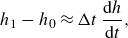 \begin{eqnarray} h_1-h_0 \approx \Delta t\, \frac {{\textrm{d}}h}{{\textrm{d}}t}, \end{eqnarray}
a dynamical understanding of what controls the boiling duration time $\Delta t$
, and the rising rate of the interface
$\Delta t$
, and the rising rate of the interface ${\textrm{d}}h/{\textrm{d}}t$
, is necessary. A closer look at the green light pixel intensity value (figure 3
c) shows an internal interface between the bottom and middle syrup layers. This internal interface appears at the onset of boiling, and its height decreases from the initial interfacial height
${\textrm{d}}h/{\textrm{d}}t$
, is necessary. A closer look at the green light pixel intensity value (figure 3
c) shows an internal interface between the bottom and middle syrup layers. This internal interface appears at the onset of boiling, and its height decreases from the initial interfacial height $h_0$
to zero at the end of boiling (dashed white line in figure 3
c). The vortex rings carry up syrup from the bottom syrup layer, mix it with the fresh water, and deposit the mixture in the middle mixed layer. Thus the bottom syrup layer gets thinner and finally disappears, letting the relatively cold middle mixed layer contact the bottom and quench the boiling. This suggests that
$h_0$
to zero at the end of boiling (dashed white line in figure 3
c). The vortex rings carry up syrup from the bottom syrup layer, mix it with the fresh water, and deposit the mixture in the middle mixed layer. Thus the bottom syrup layer gets thinner and finally disappears, letting the relatively cold middle mixed layer contact the bottom and quench the boiling. This suggests that $\Delta t$
is the time needed for vortex rings to remove the bottom syrup layer:
$\Delta t$
is the time needed for vortex rings to remove the bottom syrup layer:
 \begin{eqnarray} \Delta t \approx \frac {h_0}{\overline {w_+}}, \end{eqnarray}
where $\overline {w_+}$
(in m s
$\overline {w_+}$
(in m s $^{-1}$
) is the horizontally averaged syrup volume flux across the internal interface.
$^{-1}$
) is the horizontally averaged syrup volume flux across the internal interface.
Finally, we note that bubbles are not produced homogeneously at the beaker’s bottom. They sometimes occur successively at one spot or another (presumably due to imperfections), which may enhance the interaction between vortex rings.
4. Theory for the final layer thickness
This section builds a theoretical framework to understand how the net effect of mixing, $h_1-h_0$
, depends on the control parameters
$h_1-h_0$
, depends on the control parameters $F_s$
,
$F_s$
, $h_0$
and
$h_0$
and $S_0$
. Modelling
$S_0$
. Modelling ${\textrm{d}}h/{\textrm{d}}t$
is equivalent to modelling the ensemble effect of vortex rings. Although mixing by individual vortex rings has been investigated by Olsthoorn & Dalziel (Reference Olsthoorn and Dalziel2015), the boiling stratified flow provides a unique set-up to study the nonlinear interaction of successive vortex rings in a turbulent environment.
${\textrm{d}}h/{\textrm{d}}t$
is equivalent to modelling the ensemble effect of vortex rings. Although mixing by individual vortex rings has been investigated by Olsthoorn & Dalziel (Reference Olsthoorn and Dalziel2015), the boiling stratified flow provides a unique set-up to study the nonlinear interaction of successive vortex rings in a turbulent environment.
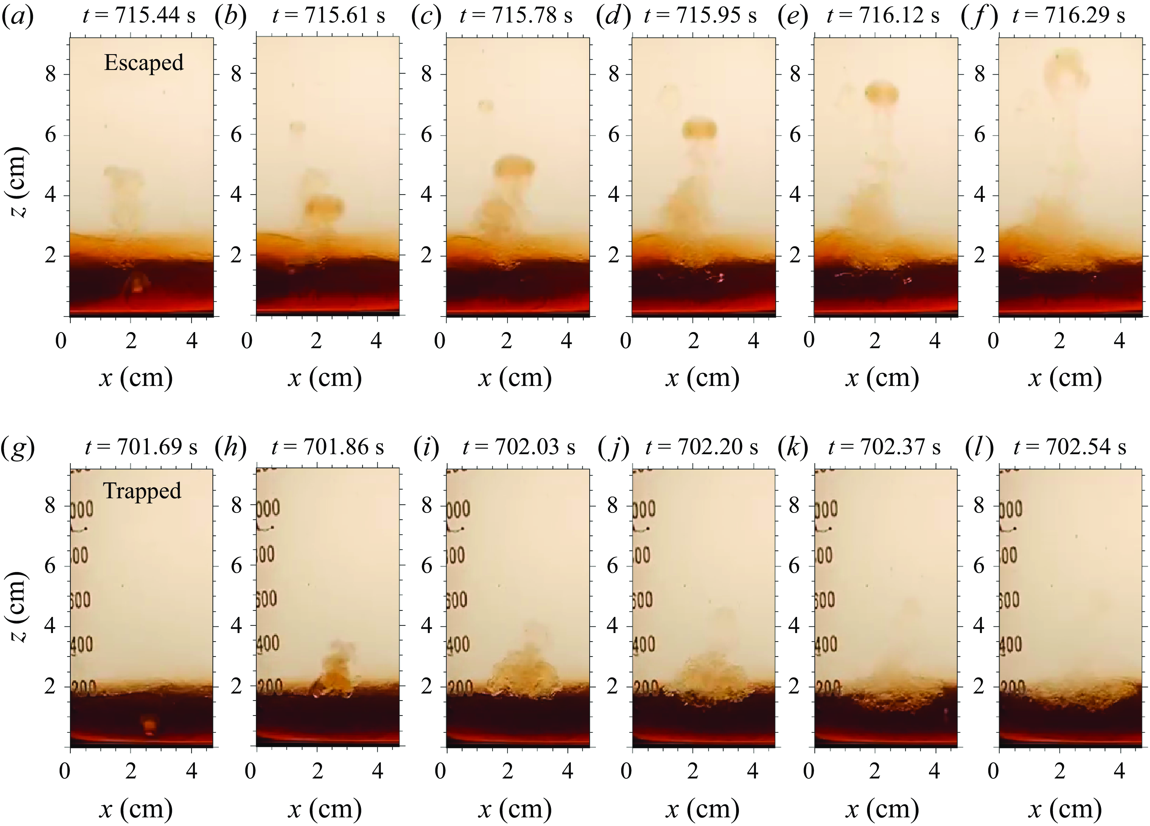
4.1. Escaped versus trapped vortex rings
Examples of the two life paths of a vortex ring in the reference experiment S3. The first row shows an escaped vortex ring, and the second row shows a trapped vortex ring, both with time interval 0.17 s between snapshots.
A schematic diagram of the two life paths of a vortex ring: escaped and trapped.
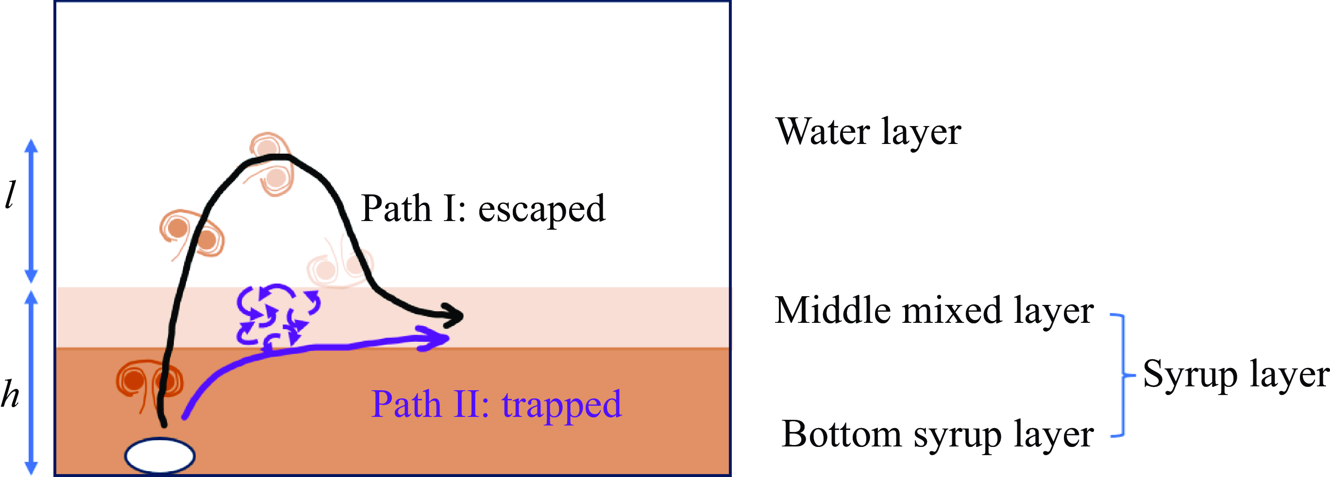
Figure 4 shows the two typical life paths of vortex rings: escaped and trapped. In the ‘escaped’ case, the bubble quenches in the syrup layer, leaving a vortex ring that rises into the water layer and sinks back to the interface. Note that some vortex rings completely dissipate in the freshwater layer. Their wake, consisting of syrup, can sink back to the interface. In the ‘trapped’ case, the initial bubble has a similar size to the escaped case, but the vortex ring crashes near the interface, producing a wide turbulent patch. The two paths are conceptualised in figure 5. The escaped case has a relatively long mixing length, characterised by the vortex ring’s penetration depth $l$
. By contrast, the trapped case has a shorter mixing length, with a limited ability to bring down the colder water. Thus we infer that the escaped vortex rings are primarily responsible for the thickening of the middle mixed layer.
$l$
. By contrast, the trapped case has a shorter mixing length, with a limited ability to bring down the colder water. Thus we infer that the escaped vortex rings are primarily responsible for the thickening of the middle mixed layer.
We define the escape ratio $E$
to quantify the fraction of vortex rings that escape the middle mixed layer and rise into the water layer. We hypothesise that stratified turbulence along the path of a vortex ring causes trapping. The turbulence can be induced by the wake of ascending vortex rings (Maxworthy Reference Maxworthy1974) or the baroclinic vorticity generated at the interface (Olsthoorn & Dalziel Reference Olsthoorn and Dalziel2018). Turbulence can tilt the direction of a vortex ring and make it propagate obliquely onto the interface. The experiments of Pinaud et al. (Reference Pinaud, Albagnac, Cazin, Rida, Anne-Archard and Brancher2021) showed that an oblique incidence could significantly tilt the vortex ring, even to a horizontal direction, due to the interaction between the vortex ring and the baroclinically generated vorticity at the interface.
$E$
to quantify the fraction of vortex rings that escape the middle mixed layer and rise into the water layer. We hypothesise that stratified turbulence along the path of a vortex ring causes trapping. The turbulence can be induced by the wake of ascending vortex rings (Maxworthy Reference Maxworthy1974) or the baroclinic vorticity generated at the interface (Olsthoorn & Dalziel Reference Olsthoorn and Dalziel2018). Turbulence can tilt the direction of a vortex ring and make it propagate obliquely onto the interface. The experiments of Pinaud et al. (Reference Pinaud, Albagnac, Cazin, Rida, Anne-Archard and Brancher2021) showed that an oblique incidence could significantly tilt the vortex ring, even to a horizontal direction, due to the interaction between the vortex ring and the baroclinically generated vorticity at the interface.
Because a vortex ring of smaller radius $R$
is more easily tilted by turbulence, and a thicker syrup layer
$R$
is more easily tilted by turbulence, and a thicker syrup layer $h_0$
increases the chance of tilting, we heuristically parametrise
$h_0$
increases the chance of tilting, we heuristically parametrise $E$
as
$E$
as
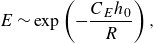 \begin{eqnarray} E \sim \exp \left ( -\frac {C_E h_0}{R} \right ), \end{eqnarray}
where $C_E$
is a non-dimensional escaping parameter depending on the turbulent kinetic energy in the syrup layer, and
$C_E$
is a non-dimensional escaping parameter depending on the turbulent kinetic energy in the syrup layer, and $R/C_E$
is a trapping length scale. The exponentially decaying function may be justified by analogy with radiative transfer: the escaping fraction of photons from an absorptive medium obeys an exponentially decaying function (the Beer–Bouguer–Lambert Law, e.g. Liou Reference Liou2002). We have not obtained an exact expression for
$R/C_E$
is a trapping length scale. The exponentially decaying function may be justified by analogy with radiative transfer: the escaping fraction of photons from an absorptive medium obeys an exponentially decaying function (the Beer–Bouguer–Lambert Law, e.g. Liou Reference Liou2002). We have not obtained an exact expression for $C_E$
, so we can only estimate its magnitude. Because both escaped and trapped vortex rings are frequently seen in our experiments, we estimate the order of magnitude of
$C_E$
, so we can only estimate its magnitude. Because both escaped and trapped vortex rings are frequently seen in our experiments, we estimate the order of magnitude of $C_E h_0 / R$
to be unity. Using
$C_E h_0 / R$
to be unity. Using $R \sim 0.5$
cm and
$R \sim 0.5$
cm and $h_0 \sim 2$
cm (figure 4), we obtain
$h_0 \sim 2$
cm (figure 4), we obtain $C_E \sim R/h_0 \sim 0.25$
. We further hypothesise that
$C_E \sim R/h_0 \sim 0.25$
. We further hypothesise that $C_E$
is higher for a higher
$C_E$
is higher for a higher $F_s$
because stronger surface heating reduces the time interval between vortex rings. The turbulent wake of the current vortex ring could trap the next one. The trapping leads to vortex ring breaking, causing stronger turbulence and therefore a pile up of vortex rings. This hypothesis will be tested in § 5 where experiments with different
$F_s$
because stronger surface heating reduces the time interval between vortex rings. The turbulent wake of the current vortex ring could trap the next one. The trapping leads to vortex ring breaking, causing stronger turbulence and therefore a pile up of vortex rings. This hypothesis will be tested in § 5 where experiments with different $F_s$
are introduced.
$F_s$
are introduced.
4.2.
The vortex ring penetration depth
$l$

Figure 6 shows that the vortex ring evolution can be divided into three stages: initial acceleration, moving in the syrup layer, and moving in the water layer. In this subsection, we first estimate the Reynolds number of the vortex ring, ${Re}_v$
, then perform a force balance analysis at each stage to derive the vortex ring penetration depth
${Re}_v$
, then perform a force balance analysis at each stage to derive the vortex ring penetration depth $l$
.
$l$
.
A schematic diagram of the vortex ring initiation and development processes, with the forces included in our model. The syrup layer includes both the bottom and middle layers. The vortex ring is neutrally buoyant in the syrup layer, and negatively buoyant in the water layer.

Most of our experiments use $S_0 \lesssim 0.6$
for the syrup layer, which has kinematic viscosity
$S_0 \lesssim 0.6$
for the syrup layer, which has kinematic viscosity $10^{-6} \lesssim \nu \lesssim 10^{-5}$
m
$10^{-6} \lesssim \nu \lesssim 10^{-5}$
m $^2$
s
$^2$
s $^{-1}$
at 80
$^{-1}$
at 80 $^\circ$
C (see Appendix B). Using a vertical velocity scale
$^\circ$
C (see Appendix B). Using a vertical velocity scale $w \sim 0.1$
m s
$w \sim 0.1$
m s $^{-1}$
and vortex ring radius
$^{-1}$
and vortex ring radius $R \sim 0.5$
cm, as estimated from the experimental result shown in figure 4, we find
$R \sim 0.5$
cm, as estimated from the experimental result shown in figure 4, we find
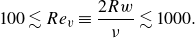 \begin{eqnarray} 100 \lesssim {Re}_v \equiv \frac {2 R w}{\nu } \lesssim 1000. \end{eqnarray}
Maxworthy (Reference Maxworthy1972) showed that a neutrally buoyant vortex ring becomes unstable and transitions to turbulence only when ${Re}_v\gtrsim 10^3$
. Thus viscosity still plays a significant role in the vortex ring dynamics.
${Re}_v\gtrsim 10^3$
. Thus viscosity still plays a significant role in the vortex ring dynamics.
The initial stage features the acceleration of the bubble by its gaseous buoyancy. A hotter surface temperature generally increases the initial bubble radius $R$
after boiling (e.g. Barathula & Srinivasan Reference Barathula and Srinivasan2022). A bubble is highly buoyant but quenches (condenses) quickly once it leaves the hot bottom. A hotter fluid interior makes the bubble condense more slowly, and yields a longer buoyancy acceleration path
$R$
after boiling (e.g. Barathula & Srinivasan Reference Barathula and Srinivasan2022). A bubble is highly buoyant but quenches (condenses) quickly once it leaves the hot bottom. A hotter fluid interior makes the bubble condense more slowly, and yields a longer buoyancy acceleration path $h_*$
. Combining these arguments, we hypothesise that
$h_*$
. Combining these arguments, we hypothesise that $h_*$
should increase with the bubble radius. For simplicity, we assume
$h_*$
should increase with the bubble radius. For simplicity, we assume
 \begin{eqnarray} h_* \approx \beta R, \end{eqnarray}
where $\beta$
is a non-dimensional bubble acceleration coefficient. Although we are unaware of how to determine the exact value of
$\beta$
is a non-dimensional bubble acceleration coefficient. Although we are unaware of how to determine the exact value of $\beta$
, the experiments provide an empirical estimate. In the experiments, most bubbles quench in the syrup layer (e.g. figure 4), so
$\beta$
, the experiments provide an empirical estimate. In the experiments, most bubbles quench in the syrup layer (e.g. figure 4), so $h_* \lesssim h_0 \approx 2$
cm. A careful observation of
$h_* \lesssim h_0 \approx 2$
cm. A careful observation of $h_*$
with a high-speed camera may be desirable in future work. Given typical bubble radius
$h_*$
with a high-speed camera may be desirable in future work. Given typical bubble radius $R \sim 0.5$
cm (e.g. figure 4), we get
$R \sim 0.5$
cm (e.g. figure 4), we get $\beta \lesssim 4$
. The vertical velocity of the vapour bubble is governed by buoyancy, perturbation pressure gradient force and viscosity:
$\beta \lesssim 4$
. The vertical velocity of the vapour bubble is governed by buoyancy, perturbation pressure gradient force and viscosity:
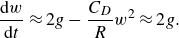 \begin{eqnarray} \frac {{\textrm{d}}w}{{\textrm{d}}t} \approx 2g - \frac {C_D}{R}w^2 \approx 2g. \end{eqnarray}
Here, the $2g$
term represents the total effect of buoyancy and the buoyancy-contributed perturbation pressure. It is a classic potential flow result (e.g. Falkovich Reference Falkovich2011, § 1.3): for a spherical bubble moving in an inviscid flow, the force implemented by the perturbation pressure on the bubble is proportional to the acceleration. The perturbation pressure originates from the inertia of the surrounding liquid forced to move with the bubble. Potential flow theory predicts that the volume of the surrounding moving fluid is half the bubble volume (figure 6), and it is therefore referred to as the ‘added mass’. Without the added mass effect, the bubble would travel much faster. The
$2g$
term represents the total effect of buoyancy and the buoyancy-contributed perturbation pressure. It is a classic potential flow result (e.g. Falkovich Reference Falkovich2011, § 1.3): for a spherical bubble moving in an inviscid flow, the force implemented by the perturbation pressure on the bubble is proportional to the acceleration. The perturbation pressure originates from the inertia of the surrounding liquid forced to move with the bubble. Potential flow theory predicts that the volume of the surrounding moving fluid is half the bubble volume (figure 6), and it is therefore referred to as the ‘added mass’. Without the added mass effect, the bubble would travel much faster. The $-(C_D/R)w^2$
term represents the total effect of viscosity and the inertia-contributed perturbation pressure, with
$-(C_D/R)w^2$
term represents the total effect of viscosity and the inertia-contributed perturbation pressure, with $C_D$
being the non-dimensional drag coefficient. The drag coefficient
$C_D$
being the non-dimensional drag coefficient. The drag coefficient $C_D$
is a function of
$C_D$
is a function of ${Re}_v$
: for a rigid sphere at
${Re}_v$
: for a rigid sphere at ${Re}_v\lesssim 10$
,
${Re}_v\lesssim 10$
, $C_D \sim 10\, {Re}_v^{-1}$
and it gradually drops to a relatively steady
$C_D \sim 10\, {Re}_v^{-1}$
and it gradually drops to a relatively steady $C_D \sim 0.2$
at
$C_D \sim 0.2$
at ${Re}_v\sim 10^3$
(Batchelor Reference Batchelor1967). For simplicity, we assume
${Re}_v\sim 10^3$
(Batchelor Reference Batchelor1967). For simplicity, we assume $C_D \sim 0.2$
, aware that the viscous effect may not be depicted accurately. Using the observed
$C_D \sim 0.2$
, aware that the viscous effect may not be depicted accurately. Using the observed $w_* \sim 0.1$
m s
$w_* \sim 0.1$
m s $^{-1}$
,
$^{-1}$
, $R\sim 0.5$
cm and
$R\sim 0.5$
cm and $C_D\sim 0.2$
, we find that the drag is negligible at the initial acceleration stage. Substituting a coordinate transform
$C_D\sim 0.2$
, we find that the drag is negligible at the initial acceleration stage. Substituting a coordinate transform ${\textrm{d}}z = w\, {\textrm{d}}t$
into (4.4) and integrating from
${\textrm{d}}z = w\, {\textrm{d}}t$
into (4.4) and integrating from $z=0$
to
$z=0$
to $z=h_*$
, we get the vertical velocity of the vortex ring
$z=h_*$
, we get the vertical velocity of the vortex ring $w_*$
as the bubble quenches:
$w_*$
as the bubble quenches:
 \begin{eqnarray} w_* \approx \left ( 4 g h_* \right )^{1/2}. \end{eqnarray}
After the bubble quenches, the surrounding moving liquid turns into a vortex ring with radius $R$
and vertical velocity
$R$
and vertical velocity $w_*$
.
$w_*$
.
In the syrup layer, the vortex ring has neutral buoyancy, influenced only by drag:
 \begin{eqnarray} \frac {{\textrm{d}}w}{{\textrm{d}}t} \approx - \frac {C_D}{R}w^2. \end{eqnarray}
Here, we use the same drag formulation as for the bubble. When the vortex ring crosses the interface, its vertical velocity $w_+$
is found by substituting
$w_+$
is found by substituting ${\textrm{d}}z = w \, {\textrm{d}}t$
into (4.6), integrating from
${\textrm{d}}z = w \, {\textrm{d}}t$
into (4.6), integrating from $z=0$
to
$z=0$
to $z=h_0$
, and using an initial condition
$z=h_0$
, and using an initial condition $w=w_*$
(see (4.5)):
$w=w_*$
(see (4.5)):
 \begin{eqnarray} w_+ = \left ( 4 g h_* \right )^{1/2} \exp \left ( -\frac {C_D h_0}{R} \right ). \end{eqnarray}
Here, the integration includes the range between $z=0$
and
$z=0$
and $z=h_*$
. This extended range not only simplifies the calculation but also compensates for the drag ignored in modelling the initial acceleration stage.
$z=h_*$
. This extended range not only simplifies the calculation but also compensates for the drag ignored in modelling the initial acceleration stage.
When the vortex ring enters the water layer, it is influenced by both drag and buoyancy. For simplicity, we consider only the buoyancy effect after the vortex ring has escaped the syrup layer. The neglect of drag in the freshwater layer is justified with a scale analysis. Using $C_D \sim 0.2$
,
$C_D \sim 0.2$
, $R\sim 0.5$
cm,
$R\sim 0.5$
cm, $w\sim 0.1$
m s
$w\sim 0.1$
m s $^{-1}$
,
$^{-1}$
, $\gamma _s=0.4$
and
$\gamma _s=0.4$
and $S_0\sim 0.5$
, the ratio of the drag term
$S_0\sim 0.5$
, the ratio of the drag term $C_D w^2/R$
to the buoyancy term
$C_D w^2/R$
to the buoyancy term $g \gamma _s S_0$
is 0.2. A smaller
$g \gamma _s S_0$
is 0.2. A smaller $S_0$
makes the approximation less valid. Because most experiments have
$S_0$
makes the approximation less valid. Because most experiments have $S_0 \gg S_{min}$
, the buoyancy is assumed to be controlled by syrup concentration rather than temperature, as discussed in § 2.1:
$S_0 \gg S_{min}$
, the buoyancy is assumed to be controlled by syrup concentration rather than temperature, as discussed in § 2.1:
 \begin{eqnarray} \frac {{\textrm{d}}w}{{\textrm{d}}t} \approx - g \gamma _s S_0. \end{eqnarray}
Substituting the initial velocity of the vortex ring entering the water layer $w_+$
from (4.7) into (4.8), we get an expression for the
$w_+$
from (4.7) into (4.8), we get an expression for the $w=0$
height of the vortex ring, which we define as the penetration depth
$w=0$
height of the vortex ring, which we define as the penetration depth $l$
:
$l$
:
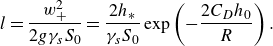 \begin{eqnarray} l = \frac {w_+^2}{2 g \gamma _s S_0} = \frac {2 h_*}{\gamma _s S_0} \exp \left (-\frac {2 C_D h_0}{R} \right ). \end{eqnarray}
The theory predicts that a more diluted syrup (smaller $S_0$
) would make the vortex ring lighter and penetrate a longer distance, and that a thicker syrup layer (higher
$S_0$
) would make the vortex ring lighter and penetrate a longer distance, and that a thicker syrup layer (higher $h_0$
) would increase the work done by drag and reduce
$h_0$
) would increase the work done by drag and reduce $l$
.
$l$
.
The penetration depth $l$
can be used to calculate the dilution of syrup carried into the water layer by the vortex ring. As shown in figure 4, both the vortex ring and its wake carry syrup. We thus call the ring and its wake ‘syrup blob’, and denote the total blob volume as
$l$
can be used to calculate the dilution of syrup carried into the water layer by the vortex ring. As shown in figure 4, both the vortex ring and its wake carry syrup. We thus call the ring and its wake ‘syrup blob’, and denote the total blob volume as $V \approx ({4}/{3}){\unicode[Arial]{x03C0}} R^3$
, where
$V \approx ({4}/{3}){\unicode[Arial]{x03C0}} R^3$
, where $R$
is the effective radius of the syrup blob, assumed to take the same radius as the vortex ring. When the buoyancy is in the same direction as the motion of the vortex ring, the vortex ring expands due to the baroclinic torque, and vice versa (Turner Reference Turner1957). Because the syrup blob experiences both updraft and downdraft stages where the buoyancy respectively decelerates and accelerates its motion, we omit the change of
$R$
is the effective radius of the syrup blob, assumed to take the same radius as the vortex ring. When the buoyancy is in the same direction as the motion of the vortex ring, the vortex ring expands due to the baroclinic torque, and vice versa (Turner Reference Turner1957). Because the syrup blob experiences both updraft and downdraft stages where the buoyancy respectively decelerates and accelerates its motion, we omit the change of $R$
due to baroclinic torque, and consider only the expansion due to entrainment. Due to the complicated structure of the blob and the low Reynolds number, the entrainment law of the blob is unclear. For simplicity, we assume that the syrup blob entrains like a turbulent vortex ring with a self-similar shape (e.g. Maxworthy Reference Maxworthy1974; Turner Reference Turner1986):
$R$
due to baroclinic torque, and consider only the expansion due to entrainment. Due to the complicated structure of the blob and the low Reynolds number, the entrainment law of the blob is unclear. For simplicity, we assume that the syrup blob entrains like a turbulent vortex ring with a self-similar shape (e.g. Maxworthy Reference Maxworthy1974; Turner Reference Turner1986):
 \begin{eqnarray} \frac {{\textrm{d}}R}{{\textrm{d}}s} = \alpha , \end{eqnarray}
where $s$
is the syrup blob’s travel distance, and
$s$
is the syrup blob’s travel distance, and $\alpha$
is the entrainment coefficient. Although we have not devised a method to determine
$\alpha$
is the entrainment coefficient. Although we have not devised a method to determine $\alpha$
from our experiments, studies on related subjects provide some references;
$\alpha$
from our experiments, studies on related subjects provide some references; $\alpha$
is approximately
$\alpha$
is approximately $O(0.01)$
for a non-buoyant vortex ring (Maxworthy Reference Maxworthy1974),
$O(0.01)$
for a non-buoyant vortex ring (Maxworthy Reference Maxworthy1974), $O(0.25)$
for a buoyant vortex ring – noting that it may be enlarged by the radius expansion due to baroclinic torque (Turner Reference Turner1957) – and
$O(0.25)$
for a buoyant vortex ring – noting that it may be enlarged by the radius expansion due to baroclinic torque (Turner Reference Turner1957) – and $O(0.1)$
for a buoyant plume (Morton et al. Reference Morton, Taylor and Turner1956). Thus we estimate
$O(0.1)$
for a buoyant plume (Morton et al. Reference Morton, Taylor and Turner1956). Thus we estimate $\alpha$
to be between
$\alpha$
to be between $O(0.01)$
and
$O(0.01)$
and $O(0.1)$
. Equation (4.10) readily shows that the expansion rate of
$O(0.1)$
. Equation (4.10) readily shows that the expansion rate of $V$
obeys
$V$
obeys
 \begin{eqnarray} \frac {1}{V} \frac {{\textrm{d}}V}{{\textrm{d}}s} = \frac {3}{R} \frac {{\textrm{d}}R}{{\textrm{d}}s} = \frac {3 \alpha }{R}. \end{eqnarray}
Next, we calculate the volume of the syrup blob when it sinks back to the interface, using the volume of the vortex ring when it first crosses the interface $V_+$
. Neglecting the horizontal moving component and considering only the vertical moving component, the syrup blob’s total travel distance is
$V_+$
. Neglecting the horizontal moving component and considering only the vertical moving component, the syrup blob’s total travel distance is $2l$
, which includes an updraft stage and a downdraft stage. Further, assuming that the syrup blob’s volume grows by only a small amount in the freshwater layer, we integrate (4.11) along the syrup blob’s trajectory to get
$2l$
, which includes an updraft stage and a downdraft stage. Further, assuming that the syrup blob’s volume grows by only a small amount in the freshwater layer, we integrate (4.11) along the syrup blob’s trajectory to get
 \begin{eqnarray} V \approx V_+ \left ( 1 + 6 \alpha \frac {l}{R} \right ), \end{eqnarray}
where $R$
is understood as the vortex ring radius when it first crosses the interface. In the next subsection, we study the rising rate of the interface due to the collective effect of many vortex rings.
$R$
is understood as the vortex ring radius when it first crosses the interface. In the next subsection, we study the rising rate of the interface due to the collective effect of many vortex rings.
4.3.
The post-boiling syrup layer thickness
$h_1$

The rising rate ${\textrm{d}}h/{\textrm{d}}t$
, where
${\textrm{d}}h/{\textrm{d}}t$
, where $h$
is the syrup layer thickness, depends on detrainment and entrainment across the syrup–water interface. Detrainment denotes the mass leaving the syrup layer, and entrainment denotes the mass entering the syrup layer. Based on the discussion in § 4.1, we consider only the thickening of the syrup layer due to the re-entry of escaped vortex rings. The mixing due to the turbulence induced by the trapped vortex rings is judged less important due to its shorter penetration depth, and is therefore neglected for simplicity. An escaped vortex ring is detrained from the syrup layer first, and then entrained. The interface height
$h$
is the syrup layer thickness, depends on detrainment and entrainment across the syrup–water interface. Detrainment denotes the mass leaving the syrup layer, and entrainment denotes the mass entering the syrup layer. Based on the discussion in § 4.1, we consider only the thickening of the syrup layer due to the re-entry of escaped vortex rings. The mixing due to the turbulence induced by the trapped vortex rings is judged less important due to its shorter penetration depth, and is therefore neglected for simplicity. An escaped vortex ring is detrained from the syrup layer first, and then entrained. The interface height $h$
obeys
$h$
obeys
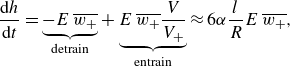 \begin{eqnarray} \frac {{\textrm{d}}h}{{\textrm{d}}t} = \underbrace { -E\, \overline {w_+} }_{\text{detrain}} + \underbrace { E\, \overline {w_+} \frac {V}{V_+} }_{\text{entrain}} \approx 6 \alpha \frac {l}{R} E\, \overline {w_+}, \end{eqnarray}
where $\overline {w_+}$
is the horizontally averaged volume flux of vortex rings from the bottom syrup layer to the middle mixed layer, and
$\overline {w_+}$
is the horizontally averaged volume flux of vortex rings from the bottom syrup layer to the middle mixed layer, and $E\,\overline {w_+}$
is the flux from the middle mixed layer to the freshwater layer, with
$E\,\overline {w_+}$
is the flux from the middle mixed layer to the freshwater layer, with $E$
representing the escape ratio of vortex rings. The ratio
$E$
representing the escape ratio of vortex rings. The ratio $V/V_+$
is calculated from (4.12).
$V/V_+$
is calculated from (4.12).
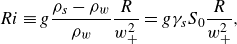
Our model is consistent with the experimental result of Olsthoorn & Dalziel (Reference Olsthoorn and Dalziel2015), who studied successive vortex rings impinging onto a stratification interface. Their experiments showed that the ratio of net entrainment to detrainment, essentially the $6 \alpha l/R$
factor in our formulation, is proportional to
$6 \alpha l/R$
factor in our formulation, is proportional to ${Ri^{-1}}$
. Here,
${Ri^{-1}}$
. Here, ${Ri}$
is the bulk Richardson number that obeys
${Ri}$
is the bulk Richardson number that obeys
 \begin{eqnarray} {Ri} \equiv g \frac {\rho _s - \rho _w}{\rho _w}\frac {R}{w^2_+} = g \gamma _s S_0 \frac {R}{w^2_+}, \end{eqnarray}
which shows ${Ri} \propto S_0$
. Substituting the expression for
${Ri} \propto S_0$
. Substituting the expression for $l$
in (4.9) into (4.13), we get
$l$
in (4.9) into (4.13), we get
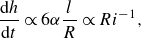 \begin{eqnarray} \frac {{\textrm{d}}h}{{\textrm{d}}t} \propto 6 \alpha \frac {l}{R} \propto {Ri}^{-1}, \end{eqnarray}
which is consistent with the ${Ri}^{-1}$
scaling of their measured entrainment rate. It is also worth noting that Wyant et al. (Reference Wyant, Bretherton, Rand and Stevens1997) proposed a similar
${Ri}^{-1}$
scaling of their measured entrainment rate. It is also worth noting that Wyant et al. (Reference Wyant, Bretherton, Rand and Stevens1997) proposed a similar ${Ri}^{-1}$
scaling for modelling the entrainment of air from the atmospheric inversion layer to the boundary layer by shallow cumuli, using the cloud depth as the length scale in calculating Ri.
${Ri}^{-1}$
scaling for modelling the entrainment of air from the atmospheric inversion layer to the boundary layer by shallow cumuli, using the cloud depth as the length scale in calculating Ri.
Combining (3.1), (3.2), (4.1), (4.9) and (4.13), we obtain an expression for $h_1$
:
$h_1$
:
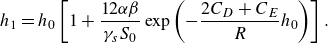 \begin{eqnarray} h_1 = h_0 \left [ 1 + \frac {12 \alpha \beta }{\gamma _s S_0} \exp \left ( - \frac {2C_D + C_E}{R} h_0 \right ) \right ]. \end{eqnarray}
Note that the mean vertical volume flux of vortex rings $\overline {w_+}$
(see (3.2)) does not appear in the expression for
$\overline {w_+}$
(see (3.2)) does not appear in the expression for $h_1$
. This expression has two unknown parameters:
$h_1$
. This expression has two unknown parameters:
-
(i)
$\alpha \beta$
, the product of the syrup blob’s entrainment parameter
$\alpha$
and the bubble acceleration parameter
$\beta$
-
(ii) the effective drag coefficient
$2C_D + C_E$
, which represents the bulk effect of the physical drag and the trapping by turbulence.


To close the theory for $ h_1$
, we still need to find an expression for the vortex ring radius
$ h_1$
, we still need to find an expression for the vortex ring radius $R$
, which is determined by the thermodynamics of boiling.
$R$
, which is determined by the thermodynamics of boiling.
4.4.
The bubble radius
$R$

The bubble radius $R$
in this experiment depends on how superheated the syrup layer temperature is (Barathula & Srinivasan Reference Barathula and Srinivasan2022). We let the syrup layer temperature be
$R$
in this experiment depends on how superheated the syrup layer temperature is (Barathula & Srinivasan Reference Barathula and Srinivasan2022). We let the syrup layer temperature be $T$
, and the boiling temperature be
$T$
, and the boiling temperature be $T_* \approx 100\,^{\circ}$
C. When
$T_* \approx 100\,^{\circ}$
C. When $T\ll T_*$
, there is no boiling, so
$T\ll T_*$
, there is no boiling, so $R=0$
. When
$R=0$
. When $T\gtrsim T_*$
, the water is superheated, and Narayan et al. (Reference Narayan, Singh and Srivastava2020) showed that
$T\gtrsim T_*$
, the water is superheated, and Narayan et al. (Reference Narayan, Singh and Srivastava2020) showed that $R$
has an upper bound with respect to
$R$
has an upper bound with respect to $T-T_*$
, which we take as
$T-T_*$
, which we take as $R_m$
. There is still uncertainty in the bubble diameter–superheating relation. Chang & Ferng (Reference Chang and Ferng2019) reported a steady increase in merged bubble diameter with the superheating temperature, though the diameter of isolated bubbles seems insensitive to superheating. For simplicity, we acknowledge the existence of the upper bound
$R_m$
. There is still uncertainty in the bubble diameter–superheating relation. Chang & Ferng (Reference Chang and Ferng2019) reported a steady increase in merged bubble diameter with the superheating temperature, though the diameter of isolated bubbles seems insensitive to superheating. For simplicity, we acknowledge the existence of the upper bound $R_m$
. Choosing
$R_m$
. Choosing $R= R_m\,\mathcal{H}(T-T_*)$
as a Heaviside function of
$R= R_m\,\mathcal{H}(T-T_*)$
as a Heaviside function of $T$
is likely sensible for an individual bubble, but there should be a smoothing factor for a group of bubbles because the temperature in the syrup layer is inhomogeneous. We may view
$T$
is likely sensible for an individual bubble, but there should be a smoothing factor for a group of bubbles because the temperature in the syrup layer is inhomogeneous. We may view $R$
as the mean bubble radius, and
$R$
as the mean bubble radius, and $T$
as the mean temperature at the bottom of the syrup layer. Suppose that the temperature obeys a Gaussian distribution with standard deviation
$T$
as the mean temperature at the bottom of the syrup layer. Suppose that the temperature obeys a Gaussian distribution with standard deviation $\delta T_*/\sqrt{2}$
. The mean bubble radius
$\delta T_*/\sqrt{2}$
. The mean bubble radius $R$
should obey an error function of
$R$
should obey an error function of $T-T_*$
:
$T-T_*$
:
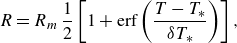 \begin{eqnarray} R = R_m \, \frac {1}{2}\left [ 1 + \text{erf} \left ( \frac {T-T_*}{\delta T_*} \right ) \right ], \end{eqnarray}
as illustrated in figure 7. A careful investigation of the temperature distribution function and $\delta T_*$
is left for future work.
$\delta T_*$
is left for future work.
A schematic diagram that illustrates the parametrisation of the bubble radius $R$
as a function of
$R$
as a function of $T$
, which is ultimately linked to the initial syrup concentration
$T$
, which is ultimately linked to the initial syrup concentration $S_0$
.
$S_0$
.
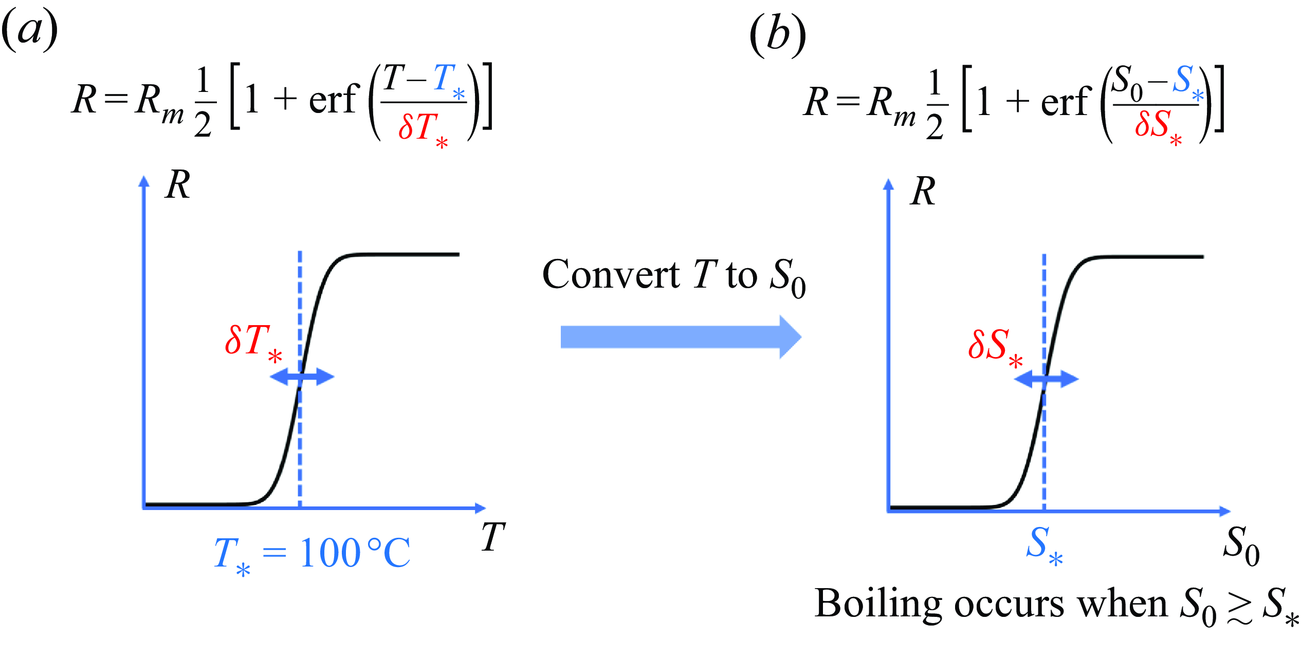
The superheating temperature $T-T_*$
is difficult to measure. However, by analysing the heat balance in the syrup layer, we can express
$T-T_*$
is difficult to measure. However, by analysing the heat balance in the syrup layer, we can express $T-T_*$
as a function of the initial syrup concentration
$T-T_*$
as a function of the initial syrup concentration $S_0$
. This is because
$S_0$
. This is because $S_0$
significantly influences the convective heat transfer rate in the syrup layer via its influence on viscosity and the density jump across the syrup–water interface. A higher
$S_0$
significantly influences the convective heat transfer rate in the syrup layer via its influence on viscosity and the density jump across the syrup–water interface. A higher $S_0$
increases the viscosity and density jump, suppressing the heat transfer. In Appendix C, we estimate the equilibrium temperature of the syrup layer by considering the balance between convective heat transfer and surface heating. The superheating temperature
$S_0$
increases the viscosity and density jump, suppressing the heat transfer. In Appendix C, we estimate the equilibrium temperature of the syrup layer by considering the balance between convective heat transfer and surface heating. The superheating temperature $T-T_*$
turns out to be a function of the syrup concentration
$T-T_*$
turns out to be a function of the syrup concentration $S_0$
, enabling us to rephrase (4.17) as
$S_0$
, enabling us to rephrase (4.17) as
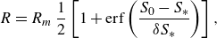 \begin{eqnarray} R = R_m \ \frac {1}{2}\left [ 1 + \textrm{erf} \left ( \frac {S_0-S_*}{\delta S_*} \right ) \right ], \end{eqnarray}
where $S_*$
is the critical syrup concentration for boiling, and
$S_*$
is the critical syrup concentration for boiling, and $\delta S_*$
is the range of syrup concentration in which the bubble radius is sensitive to
$\delta S_*$
is the range of syrup concentration in which the bubble radius is sensitive to $S_0$
(figure 7
b). Equation (4.18) indicates that a more concentrated syrup makes bubbles larger.
$S_0$
(figure 7
b). Equation (4.18) indicates that a more concentrated syrup makes bubbles larger.
Substituting (4.18) into (4.16), we finally close our heuristic theoretical model for how the final $h_1$
depends on the initial
$h_1$
depends on the initial $h_0$
and
$h_0$
and $S_0$
:
$S_0$
:
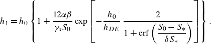 \begin{eqnarray} h_1 = h_0 \left \{ 1 + \frac {12 \alpha \beta }{\gamma _s S_0} \exp \left [ - \frac {h_0}{h_{DE}}\,\frac {2}{ 1 + \textrm{erf} \left ( \dfrac {S_0-S_*}{\delta S_*} \right ) } \right ] \right \}. \end{eqnarray}
Here, $h_{DE}$
is the vortex ring dissipation length scale:
$h_{DE}$
is the vortex ring dissipation length scale:
 \begin{eqnarray} h_{DE} \equiv \frac {R_m}{2C_D + C_E}, \end{eqnarray}
which represents the bulk effect of drag and trapping.
4.5. Summary of parameters
Our theory summarised in (4.19) has four unknown parameters: $\alpha \beta$
,
$\alpha \beta$
, $h_{DE}$
,
$h_{DE}$
, $\delta S_*$
and
$\delta S_*$
and $S_*$
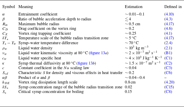
. Their order-of-magnitude estimations are summarised in table 2. With slight tuning, we find the following set of values to match almost all experimental results:
$S_*$
. Their order-of-magnitude estimations are summarised in table 2. With slight tuning, we find the following set of values to match almost all experimental results: $\alpha \beta =0.08$
,
$\alpha \beta =0.08$
, $h_{DE}=1.35$
cm,
$h_{DE}=1.35$
cm, $\delta S_*=0.05$
and
$\delta S_*=0.05$
and $S_* = 0.25$
, as will be discussed in § 5.
$S_* = 0.25$
, as will be discussed in § 5.
A summary of parameters for estimating $\alpha \beta$
,
$\alpha \beta$
, $h_{DE}$
,
$h_{DE}$
, $\delta S_*$
and
$\delta S_*$
and $S_*$
in (4.19). The basic parameters used to derive them are shown in the upper part of the table, while the magnitudes of the four final parameters are shown in the lower part.
$S_*$
in (4.19). The basic parameters used to derive them are shown in the upper part of the table, while the magnitudes of the four final parameters are shown in the lower part.
These four parameters may also be functions of the surface heat flux $F_s$
. A higher
$F_s$
. A higher $F_s$
raises the syrup layer’s turbulent kinetic energy, traps more vortex rings, increases
$F_s$
raises the syrup layer’s turbulent kinetic energy, traps more vortex rings, increases $C_E$
, and reduces
$C_E$
, and reduces $h_{DE}$
in (4.20). A higher
$h_{DE}$
in (4.20). A higher $F_s$
makes boiling easier against the convective ventilation, and reduces the critical syrup concentration for boiling
$F_s$
makes boiling easier against the convective ventilation, and reduces the critical syrup concentration for boiling $S_*$
(see (C8)). We do not have sufficient evidence to infer how
$S_*$
(see (C8)). We do not have sufficient evidence to infer how $\alpha$
and
$\alpha$
and $\beta$
depend on
$\beta$
depend on $F_s$
. Given these uncertainties, we leave the quantitative modelling of how
$F_s$
. Given these uncertainties, we leave the quantitative modelling of how $h_1$
depends on
$h_1$
depends on $F_s$
for future work.
$F_s$
for future work.
5. Experimental validation of the theory
To test our theoretical model for the post-boiling interface height $h_1$
in (4.19), this section analyses the
$h_1$
in (4.19), this section analyses the $h_1$
data diagnosed from the horizontally averaged green light pixel value in experiments with varying
$h_1$
data diagnosed from the horizontally averaged green light pixel value in experiments with varying $F_s$
,
$F_s$
, $S_0$
and
$S_0$
and $h_0$
. The diagnostic method for the interface height is detailed in Appendix A.2. Our results are shown in figures 8 and 9.
$h_0$
. The diagnostic method for the interface height is detailed in Appendix A.2. Our results are shown in figures 8 and 9.
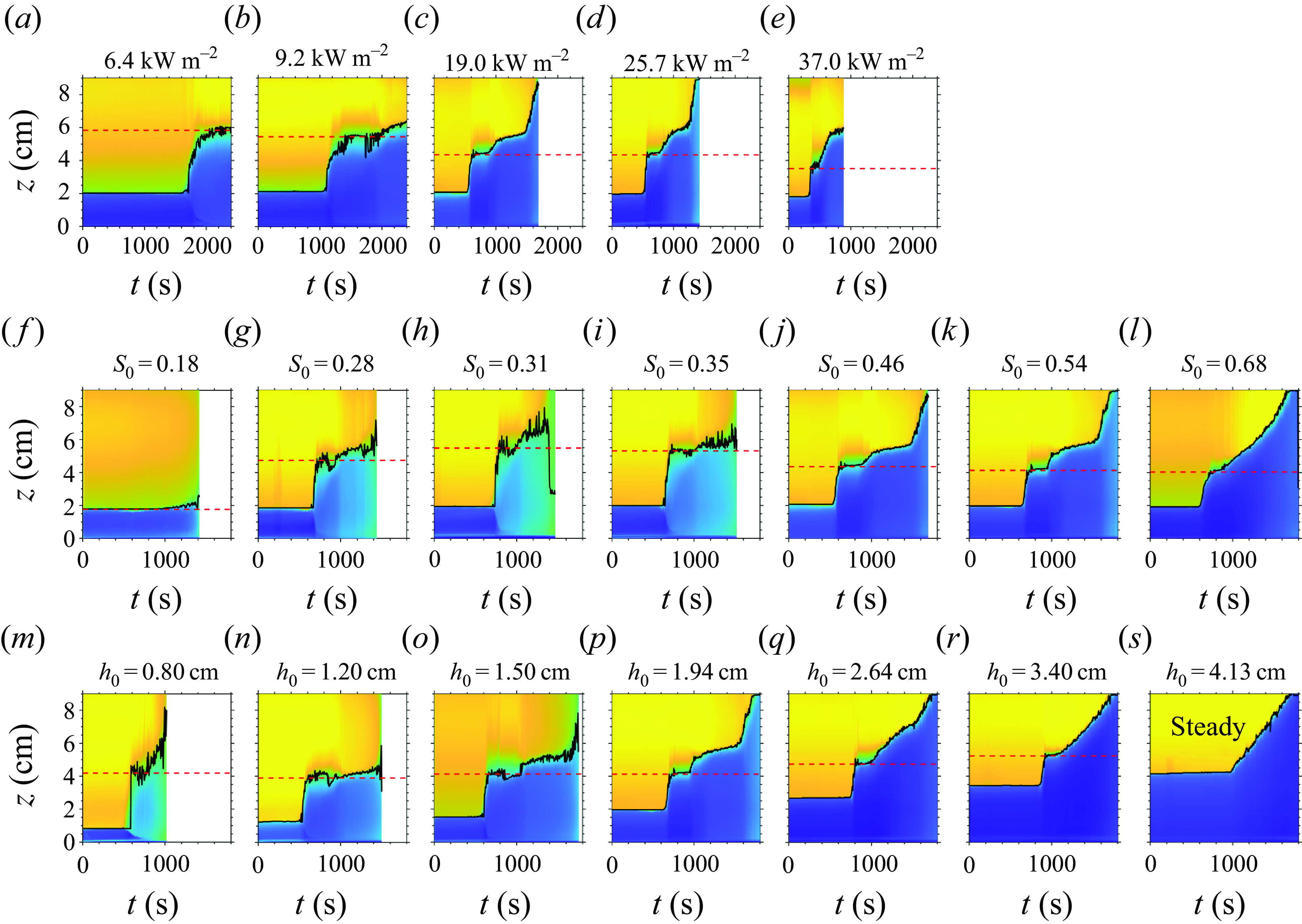
Time evolution of the syrup layer thickness shown by the video’s green pixel values. The solid black lines show the diagnosed height of the syrup–water interface, and the dashed red lines show $h_1$
. First row: experiments F1–F5, varying the surface heat flux
$h_1$
. First row: experiments F1–F5, varying the surface heat flux $F_s$
. Second row: S1–S7, varying the initial concentration
$F_s$
. Second row: S1–S7, varying the initial concentration $S_0$
. Third row: T1–T7, varying the initial thickness
$S_0$
. Third row: T1–T7, varying the initial thickness $h_0$
. In (s), T7 is in the steady boiling regime without a well-defined
$h_0$
. In (s), T7 is in the steady boiling regime without a well-defined $h_1$
. The
$h_1$
. The $h_1$
values versus
$h_1$
values versus $F_s$
,
$F_s$
, $S_0$
and
$S_0$
and $h_0$
are shown in figure 9.
$h_0$
are shown in figure 9.
Validation of the theory. The post-boiling interface height $h_1$
diagnosed from the data of figure 8 using experiments (a) F1–F5 changing
$h_1$
diagnosed from the data of figure 8 using experiments (a) F1–F5 changing $F_s$
, (b) S1–S7 changing
$F_s$
, (b) S1–S7 changing $S_0$
, and (c) T1–T6 changing
$S_0$
, and (c) T1–T6 changing $h_0$
. The blue shading in (c) shows the
$h_0$
. The blue shading in (c) shows the $h_0\lt 0.5$
cm regime where the post-boiling state lacks a clear interface, and the
$h_0\lt 0.5$
cm regime where the post-boiling state lacks a clear interface, and the $h_0\gt 4$
cm regime where the boiling is steady. The blue circles show the experimental data, and the red lines show the theoretical prediction with
$h_0\gt 4$
cm regime where the boiling is steady. The blue circles show the experimental data, and the red lines show the theoretical prediction with $\alpha \beta =0.08$
,
$\alpha \beta =0.08$
, $h_{DE}=1.35$
cm,
$h_{DE}=1.35$
cm, $\delta S_*=0.05$
and
$\delta S_*=0.05$
and $S_* = 0.25$
.
$S_* = 0.25$
.

5.1.
Experiments with varying
$F_s$

The increasing surface heat flux ( $F_s$
) in figures 8(a–e) is analogous to increasing the solar radiative heating rate on the atmospheric lower boundary. The theory (4.19) shows that
$F_s$
) in figures 8(a–e) is analogous to increasing the solar radiative heating rate on the atmospheric lower boundary. The theory (4.19) shows that $F_s$
influences
$F_s$
influences $h_1$
by two competing mechanisms.
$h_1$
by two competing mechanisms.
-
(i) A higher
$F_s$
reduces the critical syrup concentration necessary to initiate boiling,
$S_*$
(see (C8)). It should make bubbles larger and increase
$h_1$
. -
(ii) A higher
$F_s$
reduces the time interval between vortex rings and increases the turbulence intensity in the syrup layer. It should increase
$C_E$
, trap more vortex rings, reduce the entrainment of fresh water into the syrup, and decrease
$h_1$
.


Experiments show that $h_1$
decreases with
$h_1$
decreases with $F_s$
(figure 9
a). It indicates that mechanism (ii) possibly plays a more important role than mechanism (i). Future work should study why this is the case by quantitatively modelling how
$F_s$
(figure 9
a). It indicates that mechanism (ii) possibly plays a more important role than mechanism (i). Future work should study why this is the case by quantitatively modelling how $C_E$
depends on
$C_E$
depends on $F_s$
, involving a careful analysis of the interaction of vortex rings.
$F_s$
, involving a careful analysis of the interaction of vortex rings.
5.2.
Experiments with varying
$S_0$

The increasing initial syrup concentration ( $S_0$
) in figure 8(f–l) is analogous to increasing atmospheric stratification near the boundary layer top. The theory predicts that
$S_0$
) in figure 8(f–l) is analogous to increasing atmospheric stratification near the boundary layer top. The theory predicts that $S_0$
influences
$S_0$
influences $h_1$
by two competing mechanisms.
$h_1$
by two competing mechanisms.
-
(i) A higher
$S_0$
increases the viscosity. It thus reduces the convective ventilation of the syrup layer, enhances the superheating, and increases the vortex ring radius
$R$
in (4.18). A higher
$R$
makes the vortex ring less influenced by drag and trapping, allowing it to penetrate deeper, and thus increases
$h_1$
in (4.19). -
(ii) A higher
$S_0$
makes the vortex rings more negatively buoyant and penetrate less deep, and thus decreases
$h_1$
.


In the experimental results, $h_1$
first increases with
$h_1$
first increases with $S_0$
and then decreases, yielding a maximum
$S_0$
and then decreases, yielding a maximum $h_1$
for an optimal
$h_1$
for an optimal $S_0\approx 0.3$
(figure 9
b). Thus in the relatively dilute regime (
$S_0\approx 0.3$
(figure 9
b). Thus in the relatively dilute regime ( $S_0 \lesssim 0.3$
), the radius effect dominates, whereas in the relatively concentrated regime (
$S_0 \lesssim 0.3$
), the radius effect dominates, whereas in the relatively concentrated regime ( $S_0 \gtrsim 0.3$
), the buoyancy effect dominates.
$S_0 \gtrsim 0.3$
), the buoyancy effect dominates.
The red line of figure 9(b) shows the quantitative prediction of $h_1$
using (4.19). We use
$h_1$
using (4.19). We use $h_0=2$
cm. The values of the four unknown parameters are prescribed as
$h_0=2$
cm. The values of the four unknown parameters are prescribed as $\alpha \beta =0.08$
,
$\alpha \beta =0.08$
, $h_{DE}=1.35$
cm,
$h_{DE}=1.35$
cm, $\delta S_*=0.05$
,
$\delta S_*=0.05$
, $S_* = 0.25$
. This set of parameters is chosen to make the theory fit the experimental data, with their orders of magnitude justified in § 4.5. We stress that the specific parameter values are obtained from tuning, not any objective fitting method. The sensitivity to the values of the four parameters, perturbed with
$S_* = 0.25$
. This set of parameters is chosen to make the theory fit the experimental data, with their orders of magnitude justified in § 4.5. We stress that the specific parameter values are obtained from tuning, not any objective fitting method. The sensitivity to the values of the four parameters, perturbed with $\pm 20\, \%$
magnitude, is tested in the first row of figure 10, showing that the trend is robust. The optimal
$\pm 20\, \%$
magnitude, is tested in the first row of figure 10, showing that the trend is robust. The optimal $S_0$
depends mainly on
$S_0$
depends mainly on $S_*$
and
$S_*$
and $\delta S_*$
, with a higher
$\delta S_*$
, with a higher $S_*$
and higher
$S_*$
and higher $\delta S_*$
shifting the optimal
$\delta S_*$
shifting the optimal $S_0$
to larger values.
$S_0$
to larger values.
Sensitivity analysis of our theory to fitted parameter values. The first row shows the theoretical prediction of the $h_1$
versus
$h_1$
versus $S_0$
relation with perturbed parameters. The experimental results are blue circles, and the theoretical results are solid red curves. Effects are shown of (a) varying
$S_0$
relation with perturbed parameters. The experimental results are blue circles, and the theoretical results are solid red curves. Effects are shown of (a) varying $h_{DE}$
, (b) varying
$h_{DE}$
, (b) varying $\delta S_*$
, (c) varying
$\delta S_*$
, (c) varying $\alpha \beta$
, (d) varying
$\alpha \beta$
, (d) varying $S_*$
, each by a perturbation magnitude of
$S_*$
, each by a perturbation magnitude of $\pm 20\%$
. The second row is analogous but for the
$\pm 20\%$
. The second row is analogous but for the $h_1$
versus
$h_1$
versus $h_0$
relation. The blue shadings show the
$h_0$
relation. The blue shadings show the $h_0\lt 0.5$
cm and
$h_0\lt 0.5$
cm and $h_0\gt 4$
cm regimes where
$h_0\gt 4$
cm regimes where $h_1$
is not well defined.
$h_1$
is not well defined.
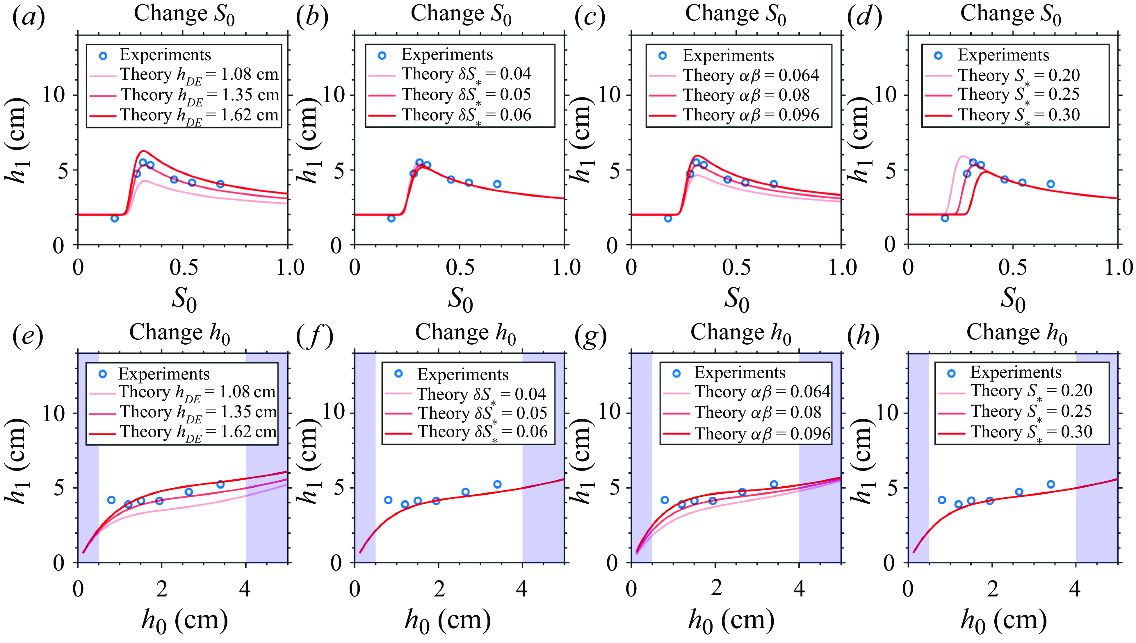
5.3. Experiments with varying
$h_0$

The increasing initial syrup thickness ( $h_0$
) in figure 8(m–s) represents increasing the atmospheric boundary layer thickness. The theory predicts that
$h_0$
) in figure 8(m–s) represents increasing the atmospheric boundary layer thickness. The theory predicts that $h_0$
influences
$h_0$
influences $h_1$
by three competing mechanisms.
$h_1$
by three competing mechanisms.
-
(i) Trivially, a higher
$h_0$
increases
$h_1$
given the same entrainment (
$h_1-h_0$
). -
(ii) A higher
$h_0$
increases the boiling duration time
$\Delta t$
because it takes longer to remove a thicker bottom syrup layer by detrainment (3.2). This effect increases
$h_1$
. -
(iii) A higher
$h_0$
increases the path for a vortex ring along which it is influenced by the drag and turbulence in the syrup layer, reducing its escape ratio
$E$
and penetration depth
$l$
(see (4.1) and (4.9)). Thus the vortex rings entrain less water, leading to a decrease of
$h_1$
.


The experimental results show that $h_1$
slightly increases with
$h_1$
slightly increases with $h_0$
(figure 9
c), indicating that the three mechanisms approximately balance each other, and a higher
$h_0$
(figure 9
c), indicating that the three mechanisms approximately balance each other, and a higher $h_0$
yields a less efficient dilution of the syrup layer by boiling. Using the same set of parameters as in § 5.2, and the measured
$h_0$
yields a less efficient dilution of the syrup layer by boiling. Using the same set of parameters as in § 5.2, and the measured $h_0$
, the trend is captured by the theory (figure 9
c). The theoretical trend is also robust in the 20 % range sensitivity tests (figure 10).
$h_0$
, the trend is captured by the theory (figure 9
c). The theoretical trend is also robust in the 20 % range sensitivity tests (figure 10).
Experiments with $h_0 \lesssim 0.5$
cm (not shown in the experimental list) yield an overly dilute post-boiling state that directly transitions to a well-mixed state. Experiments with
$h_0 \lesssim 0.5$
cm (not shown in the experimental list) yield an overly dilute post-boiling state that directly transitions to a well-mixed state. Experiments with $h_0 \lesssim 4$
cm have a clear post-boiling state, which we call the transient boiling regime. Experiments with
$h_0 \lesssim 4$
cm have a clear post-boiling state, which we call the transient boiling regime. Experiments with $h_0 \gtrsim 4$
cm, including our T7 experiment (figure 8
s), undergo continuous boiling with a steady interface rising rate, which we call the steady boiling regime. Next, we seek to understand the transition between the transient and steady regimes.
$h_0 \gtrsim 4$
cm, including our T7 experiment (figure 8
s), undergo continuous boiling with a steady interface rising rate, which we call the steady boiling regime. Next, we seek to understand the transition between the transient and steady regimes.
6. Transition between the transient and steady boiling regimes
6.1.
Solving for the transitional
$h_0$

We observed a steady boiling regime for a relatively high initial $h_0$
, a regime that is not considered in the theory of § 4. Below, we extend this theory to include the steady boiling regime, and study the transition between the transient and steady regimes.
$h_0$
, a regime that is not considered in the theory of § 4. Below, we extend this theory to include the steady boiling regime, and study the transition between the transient and steady regimes.
In the steady regime, the thick syrup layer dissipates the vortex rings sufficiently, reduces their penetrating depth, and limits the entrainment of colder water. As a result, entrainment is maintained at a rate that keeps the syrup temperature at approximately $100\,^\circ$
C:
$100\,^\circ$
C:
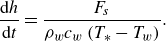 \begin{eqnarray} \frac {{\textrm{d}}h}{{\textrm{d}}t} = \frac {F_s}{\rho _w c_w \left ( T_* - T_w \right )}. \end{eqnarray}
Latent heating does not appear in (6.1) because most bubbles condense in the syrup layer. The absorption and release of latent heat balance out. Figure 8(s) shows a $\sim5$
cm rise in the interface over 800 s. Using
$\sim5$
cm rise in the interface over 800 s. Using $F_s \approx 20$
kW m
$F_s \approx 20$
kW m $^{-2}$
,
$^{-2}$
, $\rho _w c_w \approx 4\times 10^6$
J m
$\rho _w c_w \approx 4\times 10^6$
J m $^{-3}$
K
$^{-3}$
K $^{-1}$
and
$^{-1}$
and $T_*-T_w=70\,^\circ$
C, we predict from (6.1) a 5.7 cm rise over 800 s, which is consistent with the observation.
$T_*-T_w=70\,^\circ$
C, we predict from (6.1) a 5.7 cm rise over 800 s, which is consistent with the observation.
Next, we study what controls the transitional $h_0$
. If the net entrainment rate by vortex rings (shown in (4.13)) is higher than that required to keep the syrup temperature at approximately
$h_0$
. If the net entrainment rate by vortex rings (shown in (4.13)) is higher than that required to keep the syrup temperature at approximately $100\,^\circ$
C (shown in (6.1)), boiling should be transient:
$100\,^\circ$
C (shown in (6.1)), boiling should be transient:
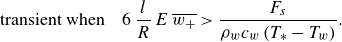 \begin{eqnarray} \textrm{transient when}\quad 6\,\frac {l}{R} \, E \, \overline {w_+} \gt \frac {F_s}{\rho _w c_w \left ( T_* - T_w \right ) }. \end{eqnarray}
Here, we must solve for the mean detrainment flux from the bottom syrup layer, $\overline {w_+}$
, a quantity that depends on the vaporisation rate at the bottom, and cancels out in solving
$\overline {w_+}$
, a quantity that depends on the vaporisation rate at the bottom, and cancels out in solving $h_1$
. Not all surface heating is used to vaporise water because the turbulent heat transfer between the bottom syrup layer and the middle mixed layer also cools the surface. We parametrise the ratio of vaporisation cooling rate to
$h_1$
. Not all surface heating is used to vaporise water because the turbulent heat transfer between the bottom syrup layer and the middle mixed layer also cools the surface. We parametrise the ratio of vaporisation cooling rate to $F_s$
as an unknown vaporisation efficiency
$F_s$
as an unknown vaporisation efficiency $\chi$
. We hypothesise that a lower vortex ring escape ratio
$\chi$
. We hypothesise that a lower vortex ring escape ratio $E$
enhances the turbulent mixing within the syrup layer, i.e. between the bottom and middle syrup layers, and reduces
$E$
enhances the turbulent mixing within the syrup layer, i.e. between the bottom and middle syrup layers, and reduces $\chi$
. The validation of this hypothesis is left for future work. The flux of bubble number density
$\chi$
. The validation of this hypothesis is left for future work. The flux of bubble number density $N$
(in m
$N$
(in m $^{-2}$
s
$^{-2}$
s $^{-1}$
), should thus obey
$^{-1}$
), should thus obey
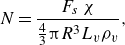 \begin{eqnarray} N = \frac {F_s \ \chi }{\frac {4}{3}\unicode{x03C0} R^3 L_v \rho _v }, \end{eqnarray}
where $L_v \approx 2.5\times 10^6$
J kg
$L_v \approx 2.5\times 10^6$
J kg $^{-1}$
is the vaporisation heat, and
$^{-1}$
is the vaporisation heat, and $\rho _v \approx 0.6$
kg m
$\rho _v \approx 0.6$
kg m $^{-3}$
is the density of vapour. The added mass argument introduced in § 4.2 indicates that the displaced volume of syrup around a bubble is half its volume (
$^{-3}$
is the density of vapour. The added mass argument introduced in § 4.2 indicates that the displaced volume of syrup around a bubble is half its volume ( ${2}/{3}\unicode{x03C0} R^3$
), hence
${2}/{3}\unicode{x03C0} R^3$
), hence
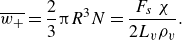 \begin{eqnarray} \overline {w_+} = \frac {2}{3}\unicode{x03C0} R^3 N = \frac {F_s \ \chi }{2L_v \rho _v}. \end{eqnarray}
We need to constrain $\chi$
from experiments. Figure 3(c) shows that the interface between the bottom syrup layer and the middle mixed layer drops from 2 cm to 0 cm in approximately 60 s, indicating
$\chi$
from experiments. Figure 3(c) shows that the interface between the bottom syrup layer and the middle mixed layer drops from 2 cm to 0 cm in approximately 60 s, indicating $\overline {w_+}\approx 3.3\times 10^{-4}$
m s
$\overline {w_+}\approx 3.3\times 10^{-4}$
m s $^{-1}$
. To fit (6.4), we constrain
$^{-1}$
. To fit (6.4), we constrain $\chi = 2 L_v \rho _v \overline {w_+} / F_s \approx 0.05$
using
$\chi = 2 L_v \rho _v \overline {w_+} / F_s \approx 0.05$
using $F_s \approx 20$
kW m
$F_s \approx 20$
kW m $^{-2}$
. Thus vaporisation should play a minor role compared to turbulent mixing in cooling the syrup layer’s bottom. In other words, the mechanical removal of superheating by mixing is more important than the phase change effect. Substituting the expressions for
$^{-2}$
. Thus vaporisation should play a minor role compared to turbulent mixing in cooling the syrup layer’s bottom. In other words, the mechanical removal of superheating by mixing is more important than the phase change effect. Substituting the expressions for $\overline {w_+}$
(6.4),
$\overline {w_+}$
(6.4), $R$
(4.18),
$R$
(4.18), $l$
(4.9) and
$l$
(4.9) and $E$
(4.1) into (6.2), we obtain the critical
$E$
(4.1) into (6.2), we obtain the critical $h_0$
for transitioning to steady boiling:
$h_0$
for transitioning to steady boiling:
 \begin{eqnarray} \textrm{steady when}\quad h_0 \gt h_{\perp } (S_0),\quad h_{\perp }(S_0) = h_{DE} \ln \left [ \frac {6 \alpha \beta \chi }{\gamma _s S_0}\, \frac {\rho _w c_w \left ( T_* - T_w \right )}{L_v \rho _v} \right ]. \end{eqnarray}
Equation (6.5) predicts that $h_{\perp }$
is linearly proportional to the dissipation length scale
$h_{\perp }$
is linearly proportional to the dissipation length scale $h_{DE}$
. The factor in the logarithm is higher for a smaller
$h_{DE}$
. The factor in the logarithm is higher for a smaller $S_0$
because a lighter syrup allows for deeper penetration and more freshwater entrainment. In deriving (6.5), we have assumed that the non-boiling regime (
$S_0$
because a lighter syrup allows for deeper penetration and more freshwater entrainment. In deriving (6.5), we have assumed that the non-boiling regime ( $S\lt S_*$
) is sufficiently separated from the steady boiling regime by letting
$S\lt S_*$
) is sufficiently separated from the steady boiling regime by letting $R=R_m$
.
$R=R_m$
.
Verification of the dependence of the transitional $h_0=h_\perp (S_0)$
separating transient and steady boiling regimes. Similar visualisation as in figure 8, but for experiments ST1–ST4 that vary both
$h_0=h_\perp (S_0)$
separating transient and steady boiling regimes. Similar visualisation as in figure 8, but for experiments ST1–ST4 that vary both $S_0$
and
$S_0$
and $h_0$
.
$h_0$
.
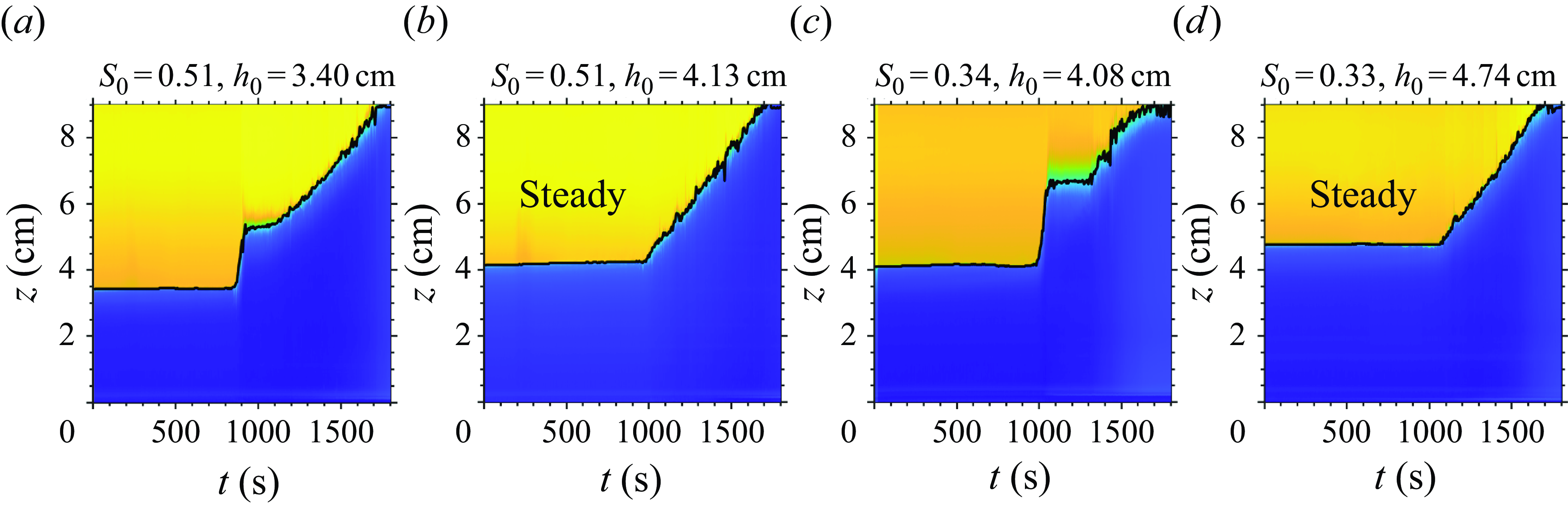
To verify the $h_{\perp } (S_0)$
dependence, we performed experiments ST1–ST4, as shown in figure 11. They use
$h_{\perp } (S_0)$
dependence, we performed experiments ST1–ST4, as shown in figure 11. They use $S_0=0.5$
and
$S_0=0.5$
and $S_0=0.35$
. Substituting in estimated values (
$S_0=0.35$
. Substituting in estimated values ( $\alpha \beta =0.08$
,
$\alpha \beta =0.08$
, $\chi =0.05$
,
$\chi =0.05$
, $\gamma _s=0.4$
,
$\gamma _s=0.4$
, $\rho _w c_w \approx 4\times 10^6$
J m
$\rho _w c_w \approx 4\times 10^6$
J m $^{-3}$
K
$^{-3}$
K $^{-1}$
,
$^{-1}$
, $T_*-T_w=70\,^\circ$
C,
$T_*-T_w=70\,^\circ$
C, $L_v=2.5\times 10^6$
J kg
$L_v=2.5\times 10^6$
J kg $^{-1}$
,
$^{-1}$
, $\rho _v=0.6$
kg m
$\rho _v=0.6$
kg m $^{-3}$
), we get
$^{-3}$
), we get $h_{\perp }(S_0=0.5) \approx 4.20$
cm and
$h_{\perp }(S_0=0.5) \approx 4.20$
cm and $h_{\perp }(S_0=0.35) \approx 4.68$
cm. For
$h_{\perp }(S_0=0.35) \approx 4.68$
cm. For $S_0 \approx 0.5$
experiments, the critical
$S_0 \approx 0.5$
experiments, the critical $h_0$
lies between
$h_0$
lies between $h_0=3.40$
cm (ST1) and
$h_0=3.40$
cm (ST1) and $h_0=4.13$
cm (ST2). For
$h_0=4.13$
cm (ST2). For $S_0 \approx 0.35$
experiments, the critical
$S_0 \approx 0.35$
experiments, the critical $h_0$
lies between
$h_0$
lies between $h_0=4.08$
cm (ST3) and
$h_0=4.08$
cm (ST3) and $h_0=4.74$
cm (ST4). Though 4.13 cm (ST2) is still slightly above 4.08 cm (ST3), the former is clearly in the steady boiling regime, and the latter is in the transient boiling regime. This confirms that a more dilute syrup yields a higher critical
$h_0=4.74$
cm (ST4). Though 4.13 cm (ST2) is still slightly above 4.08 cm (ST3), the former is clearly in the steady boiling regime, and the latter is in the transient boiling regime. This confirms that a more dilute syrup yields a higher critical $h_{\perp }$
for steady boiling, and the magnitude of theoretically predicted
$h_{\perp }$
for steady boiling, and the magnitude of theoretically predicted $h_{\perp }$
agrees with the experimental results. In summary, smaller
$h_{\perp }$
agrees with the experimental results. In summary, smaller $h_0$
and
$h_0$
and $S_0$
increase the entrainment and make boiling more transient.
$S_0$
increase the entrainment and make boiling more transient.
The system’s evolution in the syrup concentration-layer height $(S$
–
$(S$
– $h)$
phase space. Trajectories of experiments S1–S7, T1–T7 and ST1–ST4 are plotted, obeying (6.6). Blue trajectories denote the experiments with transient boiling at the first onset. Red trajectories denote the experiments with steady boiling at the first onset. The dots denote the initial
$h)$
phase space. Trajectories of experiments S1–S7, T1–T7 and ST1–ST4 are plotted, obeying (6.6). Blue trajectories denote the experiments with transient boiling at the first onset. Red trajectories denote the experiments with steady boiling at the first onset. The dots denote the initial $h=h_0$
, and the circles denote the final
$h=h_0$
, and the circles denote the final $h=h_1$
(thus trajectories ‘move up’). Note the steady and transient regimes separated by the curve
$h=h_1$
(thus trajectories ‘move up’). Note the steady and transient regimes separated by the curve $h_\perp (S_0)$
. Also note that
$h_\perp (S_0)$
. Also note that $S_{min}$
is the minimum syrup concentration for the two-layer system to be statically stable by overcoming the temperature gradient, and
$S_{min}$
is the minimum syrup concentration for the two-layer system to be statically stable by overcoming the temperature gradient, and $S_*$
is the minimum to reach the boiling point by overcoming the convective ventilation.
$S_*$
is the minimum to reach the boiling point by overcoming the convective ventilation.
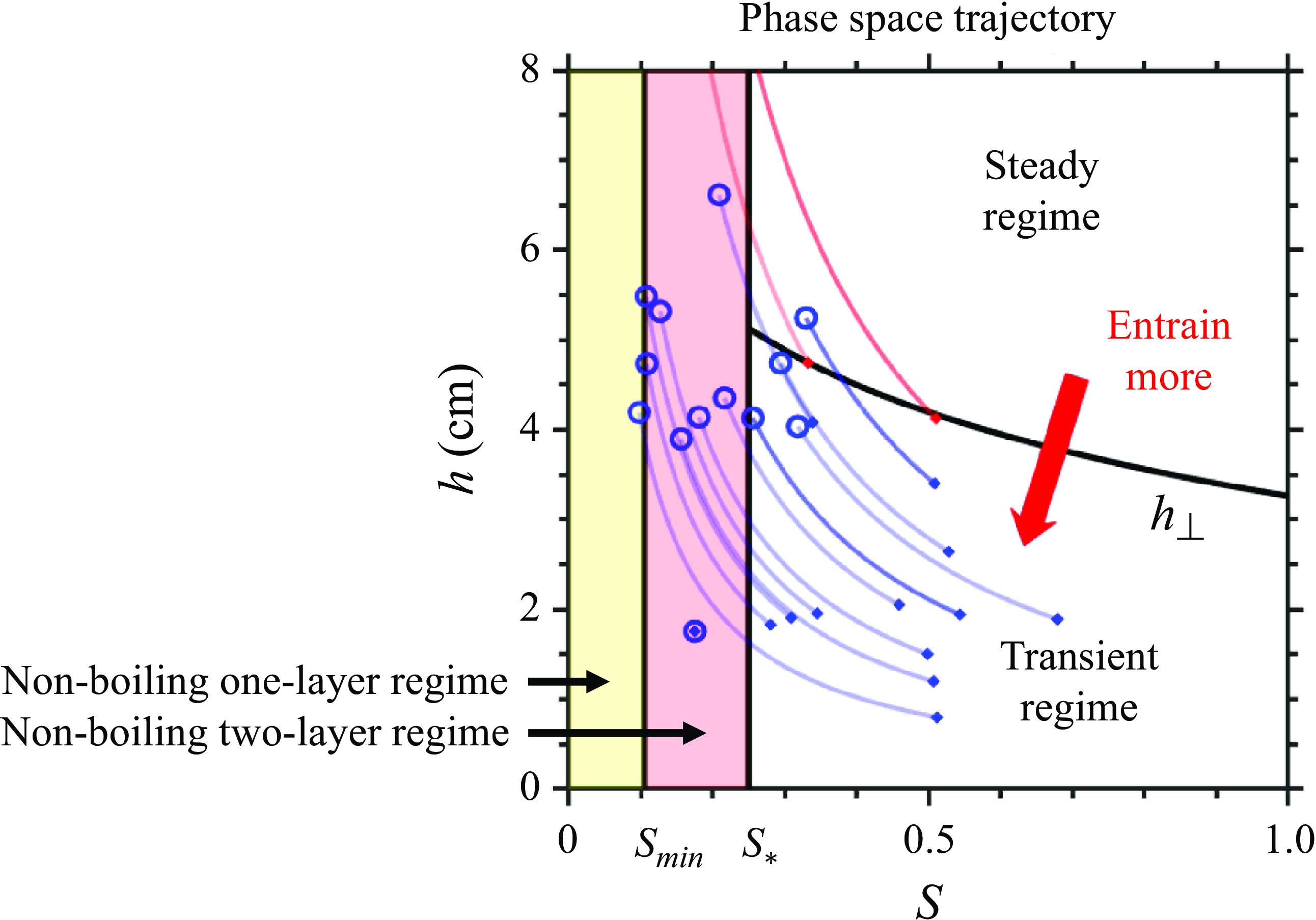
6.2. System evolution in phase space
The above discussions are for the first onset of boiling. We can analyse the second, third and even $n$
th onset using the same theory by taking the post-boiling thickness
$n$
th onset using the same theory by taking the post-boiling thickness $h_1$
as initial condition
$h_1$
as initial condition $h_0$
for the next onset. Some experiments with transient boiling at the first onset enter steady boiling after the syrup-layer temperature recovers to the boiling point. They include T5, T6 (ST1) and ST3, where either
$h_0$
for the next onset. Some experiments with transient boiling at the first onset enter steady boiling after the syrup-layer temperature recovers to the boiling point. They include T5, T6 (ST1) and ST3, where either $S_0$
or
$S_0$
or $h_0$
is relatively large (figures 8 and 11). In other experiments, the first onset of boiling makes the syrup layer too dilute to restore enough heat and boil again (i.e.
$h_0$
is relatively large (figures 8 and 11). In other experiments, the first onset of boiling makes the syrup layer too dilute to restore enough heat and boil again (i.e. $S\lt S_*$
). Here,
$S\lt S_*$
). Here, $S_*$
is the critical syrup concentration for boiling, introduced in (4.18).
$S_*$
is the critical syrup concentration for boiling, introduced in (4.18).
We summarise the system evolution in the two-dimensional phase space spanned by the instantaneous syrup concentration $S$
and syrup layer thickness
$S$
and syrup layer thickness $h$
, as shown in figure 12. Assuming that the syrup layer is diluted by entraining fresh water, and no syrup is released into the freshwater layer, there should be conservation of syrup:
$h$
, as shown in figure 12. Assuming that the syrup layer is diluted by entraining fresh water, and no syrup is released into the freshwater layer, there should be conservation of syrup:
 \begin{eqnarray} S \, h = S_0 \, h_0, \end{eqnarray}
which sets the system’s trajectory as an inverse proportional function. Note that trajectories move ‘up’ in time as $S$
decreases, while
$S$
decreases, while $h$
increases. The space is divided into four regions:
$h$
increases. The space is divided into four regions:
-
(i) the non-boiling one-layer regime (
$S\lt S_{min}$
, see yellow shading) where a two-layer configuration is convectively unstable -
(ii) the non-boiling two-layer regime (
$S_{min}\lt S\lt S_*$
, see red shading) where the convective heat transfer prevents the syrup layer from boiling -
(iii) the transient boiling regime (
$S\gt S_*$
and
$h\lt h_{\perp }$
, below the solid black curve), of primary interest in this paper -
(iv) the steady boiling regime (
$S\gt S_*$
and
$h\gt h_{\perp }$
, above the solid black curve).


We recall that expressions for $S_{min}$
and
$S_{min}$
and $h_{\perp }$
are given in (2.4) and (6.5).
$h_{\perp }$
are given in (2.4) and (6.5).
7. Discussion and conclusions
This paper has introduced a new class of experiment, boiling stratified flow, as a laboratory analogy for shallow cumulus convection. A thin syrup layer in a beaker, analogous to the atmospheric boundary layer, is heated beneath a thick freshwater layer analogous to the free troposphere. The temperature in the experiment is analogous to the water vapour mixing ratio, with the boiling exhibiting a threshold behaviour analogous to convective initiation. We summarise our fluid dynamics findings first before exploring the analogies and differences with atmospheric convection.
7.1. Fluid dynamics findings
We found that when the initial syrup concentration $S_0$
and layer thickness
$S_0$
and layer thickness $h_0$
are relatively small (but
$h_0$
are relatively small (but $S_0$
is not too small; see figure 12), the system is in a transient boiling regime. The bubbles generated at the bottom of the beaker quench on their way up and drive vortex rings that penetrate the syrup–water interface, mix with fresh water, and sink back to the interface, producing a middle mixed layer. The bottom syrup layer gradually diminishes due to the mass detrainment by vortex rings. The relatively cold middle mixed layer eventually contacts the bottom and terminates boiling. Boiling is transient because more cold water is entrained into the syrup layer than is needed to remove superheating. In this process, the syrup layer is cooled, diluted and thickened.
$S_0$
is not too small; see figure 12), the system is in a transient boiling regime. The bubbles generated at the bottom of the beaker quench on their way up and drive vortex rings that penetrate the syrup–water interface, mix with fresh water, and sink back to the interface, producing a middle mixed layer. The bottom syrup layer gradually diminishes due to the mass detrainment by vortex rings. The relatively cold middle mixed layer eventually contacts the bottom and terminates boiling. Boiling is transient because more cold water is entrained into the syrup layer than is needed to remove superheating. In this process, the syrup layer is cooled, diluted and thickened.
We constructed a phenomenological theory to model the turbulent entrainment in a boiling event, and the growth of the interface $h_1-h_0$
. Key quantities include the vortex ring escape ratio
$h_1-h_0$
. Key quantities include the vortex ring escape ratio $E$
and the vortex ring penetration depth
$E$
and the vortex ring penetration depth $l$
. The theory explains the trends observed in experiments with varying surface heat fluxes
$l$
. The theory explains the trends observed in experiments with varying surface heat fluxes $F_s$
, initial syrup concentrations
$F_s$
, initial syrup concentrations $S_0$
, and initial syrup layer heights
$S_0$
, and initial syrup layer heights $h_0$
. The post-boiling interface height
$h_0$
. The post-boiling interface height $h_1$
decreases with increasing
$h_1$
decreases with increasing $F_s$
because the higher surface heating increases the bubble number density and the turbulence in the syrup layer, which traps more vortex rings. The height
$F_s$
because the higher surface heating increases the bubble number density and the turbulence in the syrup layer, which traps more vortex rings. The height $h_1$
is non-monotonic with
$h_1$
is non-monotonic with $S_0$
, first increasing due to stronger superheating and larger bubble radius, then decreasing due to the negative buoyancy of the vortex rings. The height
$S_0$
, first increasing due to stronger superheating and larger bubble radius, then decreasing due to the negative buoyancy of the vortex rings. The height $h_1$
is relatively insensitive to
$h_1$
is relatively insensitive to $h_0$
because a thicker syrup layer makes a vortex ring more susceptible to drag and trapping, reducing its penetration depth
$h_0$
because a thicker syrup layer makes a vortex ring more susceptible to drag and trapping, reducing its penetration depth $l$
. This reduces
$l$
. This reduces $h_1-h_0$
, keeping
$h_1-h_0$
, keeping $h_1=h_0 + (h_1-h_0)$
approximately constant. Our theory for
$h_1=h_0 + (h_1-h_0)$
approximately constant. Our theory for $h_1$
accounts for the heat transfer in the syrup layer and the collective mixing effect of vortex rings. The result agrees with our experiments.
$h_1$
accounts for the heat transfer in the syrup layer and the collective mixing effect of vortex rings. The result agrees with our experiments.
By contrast, when $S_0$
and
$S_0$
and $h_0$
are relatively large, the entrainment rate drops to the minimum value needed to remove superheating in the syrup layer. This yields a steady boiling regime, where the overshooting vortex rings continuously entrain cold water into the syrup layer. By matching the transient and steady boiling theory, our transition curve predicts that smaller
$h_0$
are relatively large, the entrainment rate drops to the minimum value needed to remove superheating in the syrup layer. This yields a steady boiling regime, where the overshooting vortex rings continuously entrain cold water into the syrup layer. By matching the transient and steady boiling theory, our transition curve predicts that smaller $S_0$
raises the transitional
$S_0$
raises the transitional $h_0=h_\perp$
above which steady boiling occurs, agreeing with experiments.
$h_0=h_\perp$
above which steady boiling occurs, agreeing with experiments.
These experiments raise several fluid dynamics questions for further study. First, what determines the escape ratio $E$
? How is this quantity influenced by the interaction of vortex rings and surface heating? Second, how important is the deepening of the syrup layer by trapped vortex rings? The mixing by trapped vortex rings is considered minor compared to the mixing by escaped vortex rings. Borrowing the terminology in stratified turbulence research, the former might be considered as ‘scouring mixing’, and the latter might be considered as ‘overturning mixing’ (Caulfield Reference Caulfield2021). The relative importance of these two mixing mechanisms in boiling stratified flow should be studied further. Third, what determines the fraction of surface heating used for vaporisation
$E$
? How is this quantity influenced by the interaction of vortex rings and surface heating? Second, how important is the deepening of the syrup layer by trapped vortex rings? The mixing by trapped vortex rings is considered minor compared to the mixing by escaped vortex rings. Borrowing the terminology in stratified turbulence research, the former might be considered as ‘scouring mixing’, and the latter might be considered as ‘overturning mixing’ (Caulfield Reference Caulfield2021). The relative importance of these two mixing mechanisms in boiling stratified flow should be studied further. Third, what determines the fraction of surface heating used for vaporisation $\chi$
? It depends on the turbulence strength in the syrup layer, and may depend indirectly on
$\chi$
? It depends on the turbulence strength in the syrup layer, and may depend indirectly on $E$
. These questions lead to a more fundamental question: how does the vertical eddy diffusivity vary with height, and how can it be parametrised?
$E$
. These questions lead to a more fundamental question: how does the vertical eddy diffusivity vary with height, and how can it be parametrised?
7.2. Analogies and differences with atmospheric convection
The trends revealed by our experiments stimulate new research into atmospheric phenomena. First, the reduction of $h_1$
with increasing
$h_1$
with increasing $F_s$
reveals the dual role of turbulence in mixing. Thayer-Calder & Randall (Reference Thayer-Calder and Randall2015) proposed that the turbulence produced by downdrafts at the atmospheric boundary layer top may favour the vertical transport of moisture and heat. However, our experiments show another possibility: shallow cumulus convection, an efficient mixer, might be tilted and ‘trapped’ by turbulence. One possible future avenue would be to use large-eddy simulations to check whether this mechanism exists in the real atmosphere. Second, the optimal, intermediate
$F_s$
reveals the dual role of turbulence in mixing. Thayer-Calder & Randall (Reference Thayer-Calder and Randall2015) proposed that the turbulence produced by downdrafts at the atmospheric boundary layer top may favour the vertical transport of moisture and heat. However, our experiments show another possibility: shallow cumulus convection, an efficient mixer, might be tilted and ‘trapped’ by turbulence. One possible future avenue would be to use large-eddy simulations to check whether this mechanism exists in the real atmosphere. Second, the optimal, intermediate $S_0$
for cold-water entrainment has an analogy to the atmosphere. Parker (Reference Parker2002) studied the response of moist convection to the strength of the stratification, and found that more stable stratification suppresses not only cumulus convection, but also dry air entrainment into the boundary layer by convective cells. This leads to the build up of humidity in the boundary layer, and possibly deeper convection later on. While these analogies are encouraging, we emphasise that the boiling stratified flow differs from atmospheric moist convection in various ways, as summarised in table 3.
$S_0$
for cold-water entrainment has an analogy to the atmosphere. Parker (Reference Parker2002) studied the response of moist convection to the strength of the stratification, and found that more stable stratification suppresses not only cumulus convection, but also dry air entrainment into the boundary layer by convective cells. This leads to the build up of humidity in the boundary layer, and possibly deeper convection later on. While these analogies are encouraging, we emphasise that the boiling stratified flow differs from atmospheric moist convection in various ways, as summarised in table 3.
A summary of the comparison between the atmospheric and laboratory flows.

First, the direction of phase change is opposite to that of the atmosphere. In the experiment, buoyancy is gained by vaporisation, and lost by condensation. Latent heat is absorbed when the bubble forms, and released when the bubble quenches. Although the temperature effect on buoyancy plays a minor role compared to the bubble volume change, the analogy is less straightforward. Second, bubble nucleation in the experiment differs from the initiation of shallow cumuli by thermal bubbles in the convective boundary layer, which has regular spatial patterns (Agee & Lomax Reference Agee and Lomax1978). Their length scale has been explained with the most unstable wavelength of the (moist) Rayleigh–Bénard cell, which is related to boundary layer height (e.g. Ogura & Kondo Reference Ogura and Kondo1970; Bretherton Reference Bretherton1987; Thuburn & Efstathiou Reference Thuburn and Efstathiou2020; Öktem & Romps Reference Öktem and Romps2021). There are also convective cells in the syrup layer, but bubble formation in the experiment is more likely associated with imperfections on the beaker’s surface. A further investigation of the microphysical processes of phase change is needed. The condensation of water vapour into cloud droplets is facilitated by cloud condensation nuclei such as dust or sea salt particles (Wallace & Hobbs Reference Wallace and Hobbs2006; Rosenfeld et al. Reference Rosenfeld, Lohmann, Raga, O’Dowd, Kulmala, Fuzzi, Reissell and Andreae2008). Similarly, boiling is facilitated by boiling nuclei, such as the air bubbles on surface imperfections or suspended particles (Collier & Thome Reference Collier and Thome1994). Adding sand into the syrup solution may be pursued to explore this analogy. Third, the viscosity of the syrup layer plays an important role in suppressing the interfacial heat transfer. Atmospheric molecular viscosity is much less significant and does not play such a special role. The atmosphere has Rayleigh number ${Ra} \gtrsim 10^{16}$
(Pauluis & Schumacher Reference Pauluis and Schumacher2013), while our syrup layer has much smaller
${Ra} \gtrsim 10^{16}$
(Pauluis & Schumacher Reference Pauluis and Schumacher2013), while our syrup layer has much smaller $10^6 \lesssim {Ra} \lesssim 10^8$
(see Appendix B). Large cloud eddies have
$10^6 \lesssim {Ra} \lesssim 10^8$
(see Appendix B). Large cloud eddies have ${Re}_v\sim 10^7$
(Shaw Reference Shaw2003), while our vortex rings have
${Re}_v\sim 10^7$
(Shaw Reference Shaw2003), while our vortex rings have $10^2 \lesssim {Re}_v \lesssim 10^3$
. The high syrup viscosity also questions our theoretical vortex ring model, which applies constant drag and entrainment coefficients appropriate for a turbulent flow.
$10^2 \lesssim {Re}_v \lesssim 10^3$
. The high syrup viscosity also questions our theoretical vortex ring model, which applies constant drag and entrainment coefficients appropriate for a turbulent flow.
We refrain from drawing an analogy with deep convection and the cumulonimbus that can penetrate the troposphere, as it appears even more uncertain. Deep convection releases significant latent heat that warms the troposphere against radiative cooling, maintaining a stable stratification (Riehl & Malkus Reference Riehl and Malkus1958; Emanuel et al. Reference Emanuel, David Neelin and Bretherton1994). In our experiment, the dehydration effect of vaporisation could increase $S$
in the syrup layer, and the condensation of bubbles could reduce
$S$
in the syrup layer, and the condensation of bubbles could reduce $S$
in the freshwater layer. This process tends to enhance the buoyancy stratification, but the mass of the bubbles’ vapour is much smaller than the syrup moving with it, so the stratifying effect of boiling is much weaker than its de-stratifying effect.
$S$
in the freshwater layer. This process tends to enhance the buoyancy stratification, but the mass of the bubbles’ vapour is much smaller than the syrup moving with it, so the stratifying effect of boiling is much weaker than its de-stratifying effect.
In conclusion, although the boiling stratified flow experiment is not a generic analogue to atmospheric moist convection, it may be an enlightening model for studying the competition between convective cells and shallow cumuli in mixing. In addition, this experiment is visually striking, cost-efficient and easy to set up, and could thus be used as an educational demonstration to illustrate the feedbacks between convection, entrainment and stratification.
Acknowledgements.
We thank Y. Pu for providing experimental support at the kitchen stage of this project. We thank J. McElwaine, A. Jensen and B. Sutherland for critical experimental support. We thank Q. Kriaa, K. Burns, P. Garaud, W. Kang, D. Lohse, X. Zhang, H. Ge, Z. Kuang, Y. Si, Z. Tan, Z. Wu, W. Grabowski, H. Morrison, J. Whitehead and M. O’Neill for stimulating discussions. We appreciate the insightful comments from J.-I. Yano and two anonymous reviewers, which refined the atmospheric analogy, clarified the model, and significantly improved the manuscript.
Funding.
We acknowledge the National Science Foundation and the Office of Naval Research for their support of the 2023 WHOI Geophysical Fluid Dynamics Summer Program, where the experiments were performed. H.F. is funded by the T.C. Chamberlin Postdoctoral Fellowship at the University of Chicago. A.L. is funded by an NERC Independent Research Fellowship NE/W008971/1.
Declaration of interests.
The authors report no known conflict of interest.
Data availability statement.
Illustrative experimental videos, raw experimental videos, raw temperature records, data postprocessing codes, and a math derivation note are deposited at a dataset: https://doi.org/10.5281/zenodo.11222908.
Appendix A. Details of the experimental set-up and diagnosis method
A.1. Experimental details
The beaker (model Karter Scientific 213D20) is heated by an electric hot plate (model SUNAV-HP102-D2, 1500 W power for 110 V voltage). The heating power is controlled by a voltage regulator (brand VEVOR), which has a $\pm 2$
V fluctuation. The dark corn syrup (brand Golden Barrel) has dextrose equivalent 42 and density
$\pm 2$
V fluctuation. The dark corn syrup (brand Golden Barrel) has dextrose equivalent 42 and density $\rho _{s,max} \approx 1.4\times 10^3$
kg m
$\rho _{s,max} \approx 1.4\times 10^3$
kg m $^{-3}$
. Having tried to replace the syrup layer with a much less viscous fluid, a sodium chloride (NaCl) solution of density
$^{-3}$
. Having tried to replace the syrup layer with a much less viscous fluid, a sodium chloride (NaCl) solution of density $1.15\times 10^3$
kg m
$1.15\times 10^3$
kg m $^{-3}$
, we found that the two-layer stratification is eroded before boiling occurs.
$^{-3}$
, we found that the two-layer stratification is eroded before boiling occurs.
The illumination for imaging is provided by a desk lamp diffused by a 3 mm white acrylic sheet. The light transmitted through the beaker is recorded by the camera of an iPhone 11. The temperature is recorded with K-type thermocouples (model NUZAMAS) plugged into a temperature recorder (model Gain Express). According to the product information, the temperature resolution is 0.1 $^\circ$
C, and the accuracy is
$^\circ$
C, and the accuracy is $\pm (1\,^\circ \textrm{C}+0.3\, \%\textrm{rdg})$
between 18
$\pm (1\,^\circ \textrm{C}+0.3\, \%\textrm{rdg})$
between 18 $^\circ$
C and 28
$^\circ$
C and 28 $^\circ$
C. The four sensors are bound by heat-shrink tubes and fixed to a portable retort stand.
$^\circ$
C. The four sensors are bound by heat-shrink tubes and fixed to a portable retort stand.
The experimental procedure has three steps.
Step 1: Prepare the solution. First, we add approximately 1400 ml of tap water to the beaker. Then we use an injector to add syrup to the bottom of the beaker manually. The injecting process unavoidably causes mixing and dilutes the syrup. As a rule, the injection stops when the syrup layer reaches the required $h_0$
scale on the beaker, even if the injected syrup is less than expected. Given a desired
$h_0$
scale on the beaker, even if the injected syrup is less than expected. Given a desired $h_0$
, the volume of the syrup layer is known, but due to mixing, we use less than 100 % but typically
$h_0$
, the volume of the syrup layer is known, but due to mixing, we use less than 100 % but typically ${\gt } 75$
% of the syrup. Once the two-layer stratification is set, we use a portable resonant density meter (model Anton Paar, DMA 35) to measure the syrup density near the bottom of the beaker.
${\gt } 75$
% of the syrup. Once the two-layer stratification is set, we use a portable resonant density meter (model Anton Paar, DMA 35) to measure the syrup density near the bottom of the beaker.
Step 2: Start heating. We move the beaker onto the heating pad, and put the temperature sensor array into it. Then we turn on the heating pad, whose power is approximately fixed and controlled by the voltage regulator. The surface heat flux is measured via the temperature rising rate in a specially designed experiment using 86 V heating, 1000 ml of water, and water level height 0.077 m. The beaker is sealed on top by a plastic membrane to insulate heat. The surface heat flux at the bottom of the beaker is measured to be approximately 19 kW m $^{-2}$
. The heat flux for different voltages is calculated using Ohm’s law based on this reference value. The temperature record of this experiment and the
$^{-2}$
. The heat flux for different voltages is calculated using Ohm’s law based on this reference value. The temperature record of this experiment and the $F_s$
diagnostic code are deposited in the Zenodo dataset. The temperature record shows that it takes approximately 300 s for the heating pad to warm up and reach a steady heating power for the fluid.
$F_s$
diagnostic code are deposited in the Zenodo dataset. The temperature record shows that it takes approximately 300 s for the heating pad to warm up and reach a steady heating power for the fluid.
Step 3: Cool the device. After an experiment is finished, we cool down the heating pad to be close to the room temperature before starting another experiment. An experimental cycle takes approximately two hours.
Note that the experiments are sensitive to the geometry of the beaker. Ideally, we need a beaker whose bottom is not uniformly heated, which permits local superheating, i.e. the liquid’s temperature exceeding the boiling point. For our beaker, heating is strongest on a ring near the lateral boundary. This steady heating ring produces large bubbles that mix efficiently, leading to transient boiling. One consequence of the ring-intensified heating is that some boiling plumes are observed to crash onto the lateral wall. We have tried a 3000 ml beaker from another brand (model ULAB, UBG1029) with a more uniform surface, and an electric kettle with a perfectly uniform metal surface (model COSORI, GK172-CO). They steadily produce tiny bubbles, a regime classified as steady boiling in § 6. Because we are particularly interested in the transient boiling regime with larger bubbles, which is more relevant to cumulus clouds, we decided to use the beaker with a more non-uniform surface. Despite the sensitivity to the container, given the same beaker, the results are repeatable and robust.
A.2. Diagnostic method of the post-boiling interface height
The diagnosis of the post-boiling interface height $h_1$
has four steps.
$h_1$
has four steps.
Step 1: Calculate the horizontally averaged green light video pixel intensity value to track the interface height. The printed scale of the beaker is excluded from the averaging region.
Step 2: Identify the syrup–water interface, essentially the top of the middle mixed layer (figure 5). The interface appears as a jump of the horizontally averaged pixel intensity value in the vertical direction. To facilitate the diagnosis of the jump, we vertically smooth the pixel value with a Gaussian filter whose stencil spans 20 pixels at each time snapshot. The width of a pixel, which depends on the distance of the camera to the beaker, is approximately 0.03 cm. The height where the vertical gradient of the smoothed pixel value is the largest is identified as the interface. This operation generates a time series of the interface height $h(t)$
, shown as the solid black line in figure 8.
$h(t)$
, shown as the solid black line in figure 8.
Step 3: Identify the boiling start time. We make a temporal Gaussian filter on $h(t)$
with a stencil of 20 snapshots ( time span 101.8 s), and denote it as
$h(t)$
with a stencil of 20 snapshots ( time span 101.8 s), and denote it as $\widetilde {h}(t)$
. The initial value of
$\widetilde {h}(t)$
. The initial value of $\widetilde {h}(t)$
is taken as
$\widetilde {h}(t)$
is taken as $h_0$
. The boiling start time is taken as the time by which
$h_0$
. The boiling start time is taken as the time by which $\widetilde {h}(t)$
first rises above
$\widetilde {h}(t)$
first rises above $1.1 h_0$
.
$1.1 h_0$
.
Step 4: Identify the boiling end time using $\widetilde {h}(t)$
. We build a moving window spanning 20 snapshots (101.8 s), and move it from the boiling start time. The range (maximum minus minimum) of
$\widetilde {h}(t)$
. We build a moving window spanning 20 snapshots (101.8 s), and move it from the boiling start time. The range (maximum minus minimum) of $\widetilde {h}(t)$
in the window gradually decreases as the window approaches the post-boiling stage. We let the time by which the range first drops below 0.3 cm be the boiling end time, and denote it as
$\widetilde {h}(t)$
in the window gradually decreases as the window approaches the post-boiling stage. We let the time by which the range first drops below 0.3 cm be the boiling end time, and denote it as $h_1$
. The
$h_1$
. The $h_1$
value is shown as the dashed red line in figure 8 and summarised in figure 9. The 0.3 cm threshold provides a reasonable diagnosis of
$h_1$
value is shown as the dashed red line in figure 8 and summarised in figure 9. The 0.3 cm threshold provides a reasonable diagnosis of $h_1$
that agrees with visual inspection. There are two exceptions. One is experiment S1 (figure 8
f), where no significant boiling occurs, and the system transitions directly to a well-mixed state after a long time (approximately 1400 s). The
$h_1$
that agrees with visual inspection. There are two exceptions. One is experiment S1 (figure 8
f), where no significant boiling occurs, and the system transitions directly to a well-mixed state after a long time (approximately 1400 s). The $h_1$
value is taken as
$h_1$
value is taken as $h_0$
. The other exception is experiment T7 (figure 8
s), where boiling is steady, and no boiling end time is found.
$h_0$
. The other exception is experiment T7 (figure 8
s), where boiling is steady, and no boiling end time is found.
(a) Kinematic viscosity, (b) thermal diffusivity and (c) Prandtl number for sucrose syrup with different concentrations $S$
at
$S$
at $80\,^{\circ }\textrm{C}$
. Circles are from table A1.8 of Mohos (Reference Mohos2017), and the solid line denotes our exponential fit.
$80\,^{\circ }\textrm{C}$
. Circles are from table A1.8 of Mohos (Reference Mohos2017), and the solid line denotes our exponential fit.
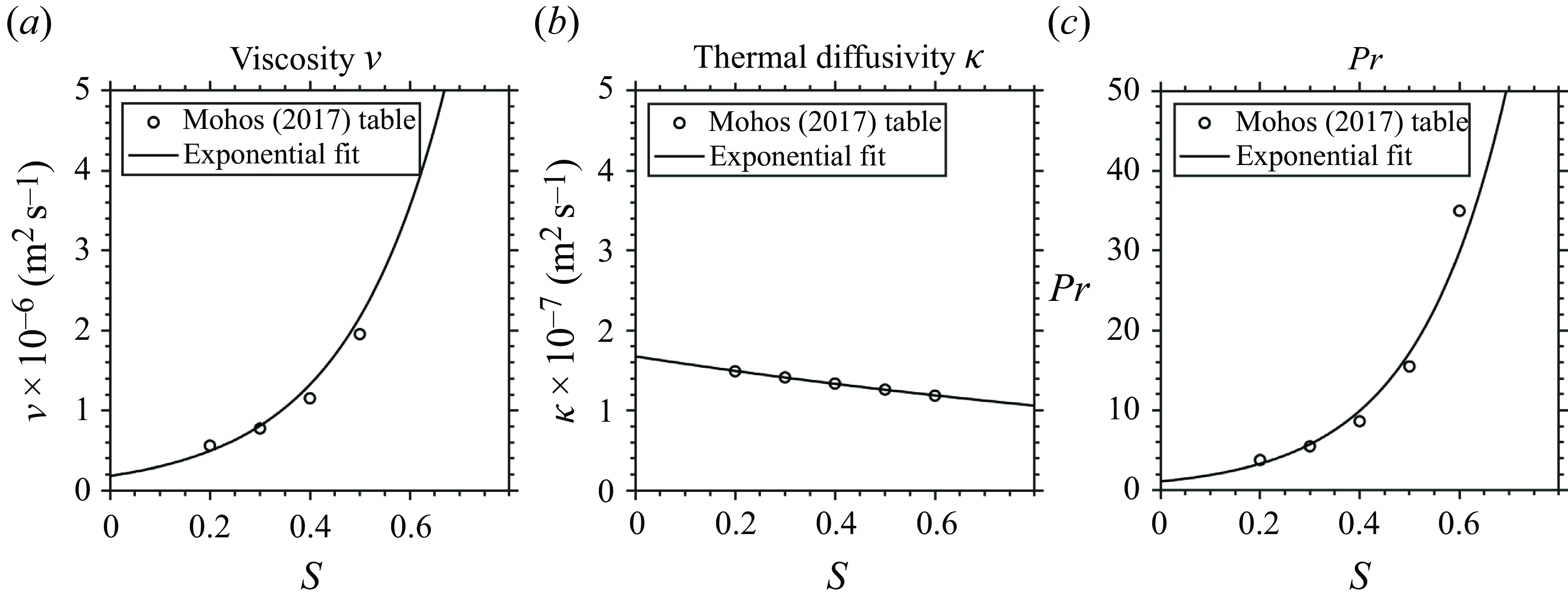
Appendix B. Rayleigh and Prandtl numbers in the syrup layer
This appendix estimates the ${Ra}$
and
${Ra}$
and ${Pr}$
values in the syrup layer. As we could not find a detailed table for our corn syrup, which is made up of glucose, we use the sucrose syrup data from Mohos (Reference Mohos2017) as a substitute. Figure 13 plots his
${Pr}$
values in the syrup layer. As we could not find a detailed table for our corn syrup, which is made up of glucose, we use the sucrose syrup data from Mohos (Reference Mohos2017) as a substitute. Figure 13 plots his $\nu ,\kappa ,{Pr}$
data (from his table A1.8) at
$\nu ,\kappa ,{Pr}$
data (from his table A1.8) at $T=80\,^{\circ }\textrm{C}$
, a typical temperature of the syrup layer before boiling. We fit these data with an exponential function of the form
$T=80\,^{\circ }\textrm{C}$
, a typical temperature of the syrup layer before boiling. We fit these data with an exponential function of the form
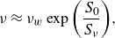 \begin{eqnarray} \nu \approx \nu _w \exp {\left (\frac {S_0}{S_{\nu }} \right )}, \end{eqnarray}
where $\nu _w=1.8\times 10^{-7}$
m
$\nu _w=1.8\times 10^{-7}$
m $^2$
s
$^2$
s $^{-1}$
is the reference kinematic viscosity of water, and
$^{-1}$
is the reference kinematic viscosity of water, and $S_{\nu }=0.2$
is the critical syrup concentration for viscosity to change significantly. The values for these two parameters were found using linear regression of
$S_{\nu }=0.2$
is the critical syrup concentration for viscosity to change significantly. The values for these two parameters were found using linear regression of $\ln \nu$
against
$\ln \nu$
against $S$
. Because the syrup viscosity reduces significantly with temperature, a syrup with
$S$
. Because the syrup viscosity reduces significantly with temperature, a syrup with $S=0.4$
at
$S=0.4$
at $80\,^{\circ }\textrm{C}$
has viscosity comparable to water at 20
$80\,^{\circ }\textrm{C}$
has viscosity comparable to water at 20 $^\circ$
C. The
$^\circ$
C. The $\kappa$
value is approximately
$\kappa$
value is approximately $1.5 \times 10^{-7}$
m
$1.5 \times 10^{-7}$
m $^2$
s
$^2$
s $^{-1}$
, and only slightly decreases with
$^{-1}$
, and only slightly decreases with $S$
.
$S$
.
Estimated ${Ra}$
and
${Ra}$
and ${Pr}$
of the syrup layer in our experiments. The blue circles, red crosses, and yellow plus signs denote experiments changing the surface heat flux
${Pr}$
of the syrup layer in our experiments. The blue circles, red crosses, and yellow plus signs denote experiments changing the surface heat flux $F_s$
, the initial syrup concentration
$F_s$
, the initial syrup concentration $S_0$
, and the initial syrup layer height
$S_0$
, and the initial syrup layer height $h_0$
, respectively.
$h_0$
, respectively.
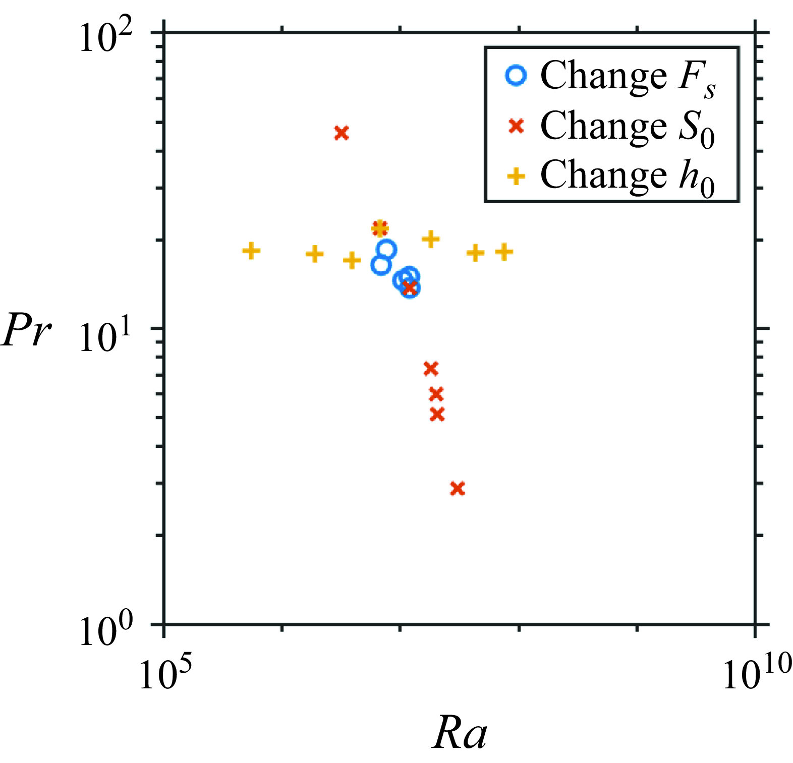
The Rayleigh number is then calculated from (C2), assuming that the syrup temperature is at the boiling temperature $T=T_*$
, and using the
$T=T_*$
, and using the $\nu$
and
$\nu$
and $\kappa$
fits. For
$\kappa$
fits. For $h_0$
and
$h_0$
and $S_0$
, we use measured values from our table 1. For the temperature difference, we use
$S_0$
, we use measured values from our table 1. For the temperature difference, we use $T_*-T_w=70\,^{\circ }\textrm{C}$
, and for the thermal expansion coefficient, we use
$T_*-T_w=70\,^{\circ }\textrm{C}$
, and for the thermal expansion coefficient, we use $\gamma _T=6\times 10^{-4}$
K
$\gamma _T=6\times 10^{-4}$
K $^{-1}$
(The Engineering ToolBox 2003). The calculation gives
$^{-1}$
(The Engineering ToolBox 2003). The calculation gives $10^6 \lesssim {Ra} \lesssim 10^8$
and
$10^6 \lesssim {Ra} \lesssim 10^8$
and $3 \lesssim {Pr} \lesssim 50$
(figure 14).
$3 \lesssim {Pr} \lesssim 50$
(figure 14).
Appendix C. Modelling heat transfer in the syrup layer
C.1. The heat transfer problem
The syrup temperature $T$
depends on the heat balance between the surface heat flux
$T$
depends on the heat balance between the surface heat flux $F_s$
, the ventilation by the interfacial heat transfer, and the vaporisation and mixing caused by boiling. For simplicity, we define this equilibrium temperature without considering boiling:
$F_s$
, the ventilation by the interfacial heat transfer, and the vaporisation and mixing caused by boiling. For simplicity, we define this equilibrium temperature without considering boiling:
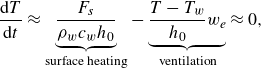 \begin{eqnarray} \frac {{\textrm{d}}T}{{\textrm{d}}t} \approx \underbrace {\frac {F_s}{\rho _w c_w h_0}}_{\text{surface heating}} - \underbrace { \frac {T-T_w}{h_0} w_e}_{\text{ventilation}} \approx 0, \end{eqnarray}
where $\rho _w \approx 10^3$
kg m
$\rho _w \approx 10^3$
kg m $^{-3}$
is the density of pure water,
$^{-3}$
is the density of pure water, $c_w \approx 4\times 10^3$
J kg
$c_w \approx 4\times 10^3$
J kg $^{-1}$
K
$^{-1}$
K $^{-1}$
is the specific heat of pure water (the volumetric heat capacity of
$^{-1}$
is the specific heat of pure water (the volumetric heat capacity of $\rho _w c_w$
could approximately represent that of syrup solution; see table A1.8 of Mohos Reference Mohos2017),
$\rho _w c_w$
could approximately represent that of syrup solution; see table A1.8 of Mohos Reference Mohos2017), $w_e$
is the characteristic eddy vertical velocity at the syrup–water interface, and
$w_e$
is the characteristic eddy vertical velocity at the syrup–water interface, and $T_w$
is the water temperature (room temperature). The syrup temperature
$T_w$
is the water temperature (room temperature). The syrup temperature $T$
could be unrealistically large without considering the cooling by boiling induced mixing. We argue that this is not a serious problem because
$T$
could be unrealistically large without considering the cooling by boiling induced mixing. We argue that this is not a serious problem because $T$
controls only the bubble radius
$T$
controls only the bubble radius $R$
, which is an error function of
$R$
, which is an error function of $T$
with an upper bound. The
$T$
with an upper bound. The $R$
value is sensitive to
$R$
value is sensitive to $T$
only where the superheating is weak and boiling is not vigorous. Thus an overestimation of
$T$
only where the superheating is weak and boiling is not vigorous. Thus an overestimation of $T$
in the vigorously boiling regime should yield little error in
$T$
in the vigorously boiling regime should yield little error in $R$
.
$R$
.
Equation (C1) shows that $T$
depends on
$T$
depends on $w_e$
, with more efficient ventilation reducing
$w_e$
, with more efficient ventilation reducing $T$
. Here, we model
$T$
. Here, we model $w_e$
with established heat transfer laws. The syrup-layer eddy is analogous to Rayleigh–Bénard convection (Bénard Reference Bénard1901; Rayleigh Reference Rayleigh1916), with the beaker’s bottom as the warm plate and the syrup–water interface as the cold plate. In our set-up, the three governing non-dimensional parameters – Rayleigh number (Ra), Nusselt number (Nu) and Prandtl number (Pr) – are defined as
$w_e$
with established heat transfer laws. The syrup-layer eddy is analogous to Rayleigh–Bénard convection (Bénard Reference Bénard1901; Rayleigh Reference Rayleigh1916), with the beaker’s bottom as the warm plate and the syrup–water interface as the cold plate. In our set-up, the three governing non-dimensional parameters – Rayleigh number (Ra), Nusselt number (Nu) and Prandtl number (Pr) – are defined as
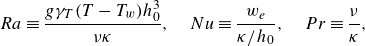 \begin{eqnarray} {Ra} \equiv \frac {g\gamma _T (T-T_w) h_0^3}{\nu \kappa }, \quad {Nu} \equiv \frac {w_e}{\kappa / h_0}, \quad {Pr} \equiv \frac {\nu }{\kappa }, \end{eqnarray}
where $\nu$
is the kinematic viscosity, and
$\nu$
is the kinematic viscosity, and $\kappa$
is the thermal diffusivity. The Ra value represents the relative strength of convective instability and the diffusive damping, and Nu represents the ratio of convective to conductive heat transfer. For syrup,
$\kappa$
is the thermal diffusivity. The Ra value represents the relative strength of convective instability and the diffusive damping, and Nu represents the ratio of convective to conductive heat transfer. For syrup, $\kappa$
is insensitive to
$\kappa$
is insensitive to $S_0$
, but
$S_0$
, but $\nu$
increases significantly with
$\nu$
increases significantly with $S_0$
and approximately obeys an exponential function (Appendix B). In Appendix B, we estimated Ra and Pr and found that most experiments have
$S_0$
and approximately obeys an exponential function (Appendix B). In Appendix B, we estimated Ra and Pr and found that most experiments have $10^6 \lesssim {Ra} \lesssim 10^8$
and
$10^6 \lesssim {Ra} \lesssim 10^8$
and $3 \lesssim {Pr} \lesssim 50$
.
$3 \lesssim {Pr} \lesssim 50$
.
Note that the syrup–water interface is only an approximation to the rigid lid. There is an additional non-dimensional parameter: the stability parameter $S/S_{min}$
. It is the ratio of the syrup concentration factor and temperature factor in the density jump across the interface. Here,
$S/S_{min}$
. It is the ratio of the syrup concentration factor and temperature factor in the density jump across the interface. Here, $S_{min}$
(defined in (2.4)) is the minimum syrup concentration needed to make the syrup–water set-up statically stable against the temperature effect. Because
$S_{min}$
(defined in (2.4)) is the minimum syrup concentration needed to make the syrup–water set-up statically stable against the temperature effect. Because $S_{min} \sim 0.1$
, most of our experiments have
$S_{min} \sim 0.1$
, most of our experiments have $2 \lesssim S_0/S_{min} \lesssim 6$
. According to Turner (Reference Turner1965), who used saltwater and a slightly higher
$2 \lesssim S_0/S_{min} \lesssim 6$
. According to Turner (Reference Turner1965), who used saltwater and a slightly higher ${Ra}\sim 10^8$
,
${Ra}\sim 10^8$
, ${Nu}$
decreases by a factor of 3 as
${Nu}$
decreases by a factor of 3 as $S_0/S_{min}$
increases from approximately 3 to approximately 6. Gonzalez-Juez et al. (Reference Gonzalez-Juez, Kerstein and Lignell2011) used a one-dimensional turbulence model to study a similar set-up, and found a power-law decay of
$S_0/S_{min}$
increases from approximately 3 to approximately 6. Gonzalez-Juez et al. (Reference Gonzalez-Juez, Kerstein and Lignell2011) used a one-dimensional turbulence model to study a similar set-up, and found a power-law decay of ${Nu}$
with the stability parameter (
${Nu}$
with the stability parameter ( $S_0/S_{min}$
). For convenience, we approximate it as an exponential decay
$S_0/S_{min}$
). For convenience, we approximate it as an exponential decay ${Nu}\sim \exp (-S_0/S_d)$
, where
${Nu}\sim \exp (-S_0/S_d)$
, where $S_d$
is the characteristic syrup concentration for the stability factor to influence heat transfer. Using the data in figure 4 of Turner (Reference Turner1965), we estimate
$S_d$
is the characteristic syrup concentration for the stability factor to influence heat transfer. Using the data in figure 4 of Turner (Reference Turner1965), we estimate $S_d \sim 0.3$
. As for the
$S_d \sim 0.3$
. As for the ${Pr}$
dependence, Gonzalez-Juez et al. (Reference Gonzalez-Juez, Kerstein and Lignell2011) found that
${Pr}$
dependence, Gonzalez-Juez et al. (Reference Gonzalez-Juez, Kerstein and Lignell2011) found that ${Nu}$
is insensitive to
${Nu}$
is insensitive to ${Pr}$
for
${Pr}$
for $3 \lesssim {Pr} \lesssim 100$
. As for the Ra dependence, both Turner (Reference Turner1965) and Gonzalez-Juez et al. (Reference Gonzalez-Juez, Kerstein and Lignell2011) found
$3 \lesssim {Pr} \lesssim 100$
. As for the Ra dependence, both Turner (Reference Turner1965) and Gonzalez-Juez et al. (Reference Gonzalez-Juez, Kerstein and Lignell2011) found ${Nu}\sim {Ra}^{1/3}$
. Thus we express Nu as
${Nu}\sim {Ra}^{1/3}$
. Thus we express Nu as
 \begin{eqnarray} {Nu} \approx c \exp \left ( -\frac {S_0}{S_d} \right ) {Ra}^{1/3}, \end{eqnarray}
where $c \sim 0.04$
is a constant inferred from the heat transfer measurement reported in figure 4 of Turner (Reference Turner1965). We warn that the Turner (Reference Turner1965) experiment uses saltwater rather than syrup concentration. Unlike syrup, saltwater does not have a significant viscosity difference compared to fresh water. Turner (Reference Turner1986) showed that a viscous contrast across an interface suppresses heat transfer. This factor, which may amplify the sensitivity of Nu to
$c \sim 0.04$
is a constant inferred from the heat transfer measurement reported in figure 4 of Turner (Reference Turner1965). We warn that the Turner (Reference Turner1965) experiment uses saltwater rather than syrup concentration. Unlike syrup, saltwater does not have a significant viscosity difference compared to fresh water. Turner (Reference Turner1986) showed that a viscous contrast across an interface suppresses heat transfer. This factor, which may amplify the sensitivity of Nu to $S_0$
, is not included in (C3). The dependence of Nu on the molecular diffusivity of syrup, which may potentially depend on
$S_0$
, is not included in (C3). The dependence of Nu on the molecular diffusivity of syrup, which may potentially depend on $S_0$
, is also not considered.
$S_0$
, is also not considered.
C.2. Derivation of the superheating temperature with
${Nu} \propto {Ra}^{1/3}$

Substituting (C3) into the definition of Nu in (C2), we obtain an expression for $w_e$
:
$w_e$
:
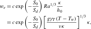 \begin{align} w_e &= c \exp \left ( -\frac {S_0}{S_d} \right ) {Ra}^{1/3} \frac {\kappa }{h_0} \nonumber \\ &= c \exp \left ( -\frac {S_0}{S_d} \right ) \left [ \frac {g \gamma _T (T-T_w)}{\nu \kappa } \right ]^{1/3} \kappa , \end{align}
which depends on $T-T_w$
,
$T-T_w$
, $\nu$
and
$\nu$
and $\kappa$
. Substituting (B1) into (C4), we get
$\kappa$
. Substituting (B1) into (C4), we get
 \begin{eqnarray} w_e = w_{e,{ref}} \exp \left [ - S_0 \left ( \frac {1}{S_d} + \frac {1}{3 S_{\nu }} \right ) \right ], \quad w_{e,{ref}} \equiv c \left [ \frac {g\gamma _T (T-T_w)}{\nu _w } \right ]^{1/3} \kappa ^{2/3}, \end{eqnarray}
where $w_{e,{ref}}$
is a reference eddy velocity scale for
$w_{e,{ref}}$
is a reference eddy velocity scale for $S_0=0$
(water). Equations (C5) indicate that a more concentrated syrup suppresses heat transfer via the density jump and viscous effect. For convenience, we define
$S_0=0$
(water). Equations (C5) indicate that a more concentrated syrup suppresses heat transfer via the density jump and viscous effect. For convenience, we define $S_{\nu d}$
to represent their bulk effect:
$S_{\nu d}$
to represent their bulk effect:
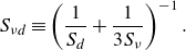 \begin{eqnarray} S_{\nu d} \equiv \left ( \frac {1}{S_d} + \frac {1}{3 S_{\nu }} \right )^{-1}. \end{eqnarray}
Appendix B shows that $S_{\nu } \sim 0.2$
. Combining it with
$S_{\nu } \sim 0.2$
. Combining it with $S_d \sim 0.3$
, we obtain
$S_d \sim 0.3$
, we obtain $S_{\nu d}\sim 0.2$
.
$S_{\nu d}\sim 0.2$
.
Now we solve the critical syrup concentration for boiling $S_*$
. Applying
$S_*$
. Applying $T=T_*$
to the temperature balance equation (C1), and substituting in (C5), we obtain
$T=T_*$
to the temperature balance equation (C1), and substituting in (C5), we obtain
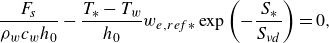 \begin{eqnarray} \frac {F_s}{\rho _w c_w h_0} - \frac {T_* - T_w}{h_0} w_{e,{ref}*} \exp \left ( - \frac {S_*}{S_{\nu d}} \right ) = 0, \end{eqnarray}
which yields an expression for $S_*$
:
$S_*$
:
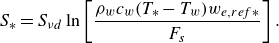 \begin{eqnarray} S_* = S_{\nu d} \ln \left [ \frac {\rho _w c_w (T_*-T_w) w_{e,{ref}*}}{F_s} \right ]. \end{eqnarray}
Here, $w_{e,{ref}*}$
is
$w_{e,{ref}*}$
is $w_{e,{ref}}$
at
$w_{e,{ref}}$
at $T=T_*$
:
$T=T_*$
:
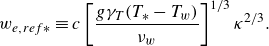 \begin{eqnarray} w_{e,{ref}*} \equiv c \left [ \frac {g\gamma _T (T_*-T_w)}{\nu _w } \right ]^{1/3} \kappa ^{2/3}. \end{eqnarray}
With $S_*$
at hand, we can solve for the superheating temperature with a perturbation analysis. Consider temperature as a small perturbation to
$S_*$
at hand, we can solve for the superheating temperature with a perturbation analysis. Consider temperature as a small perturbation to $T_*$
, and the syrup concentration as a small perturbation to
$T_*$
, and the syrup concentration as a small perturbation to $S_*$
:
$S_*$
:
 \begin{eqnarray} T^{\prime} \equiv T-T_*, \quad S_0^{\prime} \equiv S_0 - S_*, \end{eqnarray}
with $T^{\prime} \ll T_*$
and
$T^{\prime} \ll T_*$
and $S_0^{\prime} \ll S_*$
. Substituting (C5) and (C10) into the temperature balance equation (C1), we get
$S_0^{\prime} \ll S_*$
. Substituting (C5) and (C10) into the temperature balance equation (C1), we get
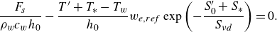 \begin{eqnarray} \frac {F_s}{\rho _w c_w h_0} - \frac {T^{\prime} + T_* - T_w}{h_0} w_{e,{ref}} \exp \left ( - \frac {S_0^{\prime} + S_*}{S_{\nu d}} \right ) = 0. \end{eqnarray}
Subtracting (C7) from (C11), using the Taylor expansion
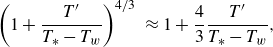 \begin{eqnarray} \left ( 1 + \frac {T^{\prime}}{T_* - T_w} \right )^{4/3} &&\approx 1 + \frac {4}{3} \frac {T^{\prime}}{T_* - T_w}, \end{eqnarray}
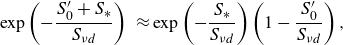 \begin{eqnarray} \exp \left ( - \frac {S_0^{\prime} + S_*}{S_{\nu d}} \right ) &&\approx \exp \left ( - \frac {S_*}{S_{\nu d}} \right ) \left ( 1 - \frac {S_0^{\prime}}{S_{\nu d}} \right ), \end{eqnarray}
and neglecting the product of the perturbation terms, we obtain the relationship between the superheating temperature ( $T - T_*$
) and the supercritical syrup concentration (
$T - T_*$
) and the supercritical syrup concentration ( $S_0-S_*$
):
$S_0-S_*$
):
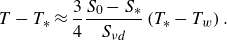 \begin{eqnarray} T - T_* \approx \frac {3}{4} \frac {S_0 - S_*}{ S_{\nu d}} \left ( T_* - T_w \right ). \end{eqnarray}
For $S_0 \gt S_*$
, convective heat transfer is too weak to keep the syrup temperature steady and below the boiling point, so boiling must occur.
$S_0 \gt S_*$
, convective heat transfer is too weak to keep the syrup temperature steady and below the boiling point, so boiling must occur.
Substituting (C14) into (4.17), we express $R$
as a function of
$R$
as a function of $S_0$
:
$S_0$
:
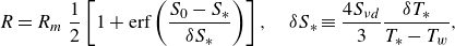 \begin{eqnarray} R = R_m \ \frac {1}{2}\left [ 1 + \textrm{erf} \left ( \frac {S_0-S_*}{\delta S_*} \right ) \right ], \quad \delta S_* \equiv \frac {4 S_{\nu d}}{3} \frac {\delta T_*}{T_* - T_w} , \end{eqnarray}
where $\delta S_*$
denotes the range of
$\delta S_*$
denotes the range of $S_0$
that can significantly influence the bubble radius (figure 7
b). Though (C15) is derived with a small-perturbation assumption, it should be valid even if the perturbation is large since erf makes
$S_0$
that can significantly influence the bubble radius (figure 7
b). Though (C15) is derived with a small-perturbation assumption, it should be valid even if the perturbation is large since erf makes $R$
sensitive to temperature only when it is around
$R$
sensitive to temperature only when it is around $T_*$
. To see how sensitive (4.18) is to the uncertain heat transfer law (C3), we generalise the result to an arbitrary power dependence of
$T_*$
. To see how sensitive (4.18) is to the uncertain heat transfer law (C3), we generalise the result to an arbitrary power dependence of ${Nu}$
on
${Nu}$
on ${Ra}$
and
${Ra}$
and ${Pr}$
in the next subsection. The
${Pr}$
in the next subsection. The $R$
still appears in the form of the erf of
$R$
still appears in the form of the erf of $(S_0-S_*)$
; only the expressions for
$(S_0-S_*)$
; only the expressions for $S_*$
and
$S_*$
and $\delta S_*$
are modified.
$\delta S_*$
are modified.
C.3. Derivation with an arbitrary heat transfer law
Because the heat transfer law in our set-up has some uncertainties, we derive the dependence of bubble radius $R$
on
$R$
on $S_0$
in a more general way, assuming a universal heat transfer law
$S_0$
in a more general way, assuming a universal heat transfer law
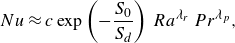 \begin{eqnarray} {Nu} \approx c \exp \left ( -\frac {S_0}{S_d} \right )\, {Ra}^{\lambda _r}\, {Pr}^{\lambda _p}, \end{eqnarray}
where $\lambda _r$
and
$\lambda _r$
and $\lambda _p$
are exponents of
$\lambda _p$
are exponents of ${Ra}$
and
${Ra}$
and ${Pr}$
, with
${Pr}$
, with $\lambda _r=1/3$
and
$\lambda _r=1/3$
and $\lambda _p=0$
being used in § C.2. We will show that the structure of
$\lambda _p=0$
being used in § C.2. We will show that the structure of $R$
as proportional to the erf of
$R$
as proportional to the erf of $S_0$
is unchanged in (C15), but the expressions for
$S_0$
is unchanged in (C15), but the expressions for $S_*$
and
$S_*$
and $\delta S_*$
are revised.
$\delta S_*$
are revised.
Substituting (C16) into (C3), we obtain
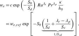 \begin{align} w_e &= c \exp \left ( -\frac {S_0}{S_d} \right )\, {Ra}^{\lambda _r}\, {Pr}^{\lambda _p}\, \frac {\kappa }{h_0} \nonumber \\ &= w_{e,{ref}} \exp \left [ - S_0 \underbrace { \left ( \dfrac {1}{S_d} + \dfrac {\lambda _r - \lambda _p}{S_{\nu }} \right ) }_{1/S_{\nu d}} \right ], \end{align}
where the expression for $S_{\nu d}$
has been revised, and
$S_{\nu d}$
has been revised, and $w_{e,{ref}}$
obeys
$w_{e,{ref}}$
obeys
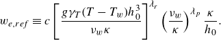 \begin{eqnarray} w_{e,{ref}} \equiv c \left [ \frac {g \gamma _T (T-T_w) h_0^3}{\nu _w \kappa } \right ]^{\lambda _r} \left ( \frac {\nu _w}{\kappa } \right )^{\lambda _p} \frac {\kappa }{h_0}. \end{eqnarray}
Substituting (C17) and (C18) into the temperature balance equation at $T=T_*$
in (C7) and at
$T=T_*$
in (C7) and at $T=T_* + T^{\prime}$
in (C11), and performing Taylor expansion, we obtain the expression for bubble radius, which has the same structure as (C15),
$T=T_* + T^{\prime}$
in (C11), and performing Taylor expansion, we obtain the expression for bubble radius, which has the same structure as (C15),
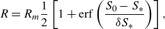 \begin{eqnarray} R = R_m \frac {1}{2}\left [ 1 + \textrm{erf} \left ( \frac {S_0-S_*}{\delta S_*} \right ) \right ], \end{eqnarray}
but the expressions for $\delta S_*$
and
$\delta S_*$
and $S_*$
are revised. The expression for
$S_*$
are revised. The expression for $\delta S_*$
is
$\delta S_*$
is
 \begin{eqnarray} \delta S_* \equiv ( 1 + \lambda _r ) S_{\nu d} \frac {\delta T_*}{T_* - T_w}, \end{eqnarray}
with
 \begin{eqnarray} S_{\nu d} \equiv \left ( \frac {1}{S_d} + \frac {\lambda _r-\lambda _p}{S_{\nu }} \right )^{-1}. \end{eqnarray}
The expression for $S_*$
is
$S_*$
is
 \begin{eqnarray} S_* = S_{\nu d} \ln \left [ \frac {\rho _w c_w (T_*-T_w) w_{e,{ref}*}}{F_s} \right ], \end{eqnarray}
with
 \begin{eqnarray} w_{e,{ref}*} \equiv c \left [ \frac {g \gamma _T (T_*-T_w) h_0^3}{\nu _w \kappa } \right ]^{\lambda _r} \left ( \frac {\nu _w}{\kappa } \right )^{\lambda _p} \frac {\kappa }{h_0}. \end{eqnarray}
Using $\lambda _{r}=1/3$
and
$\lambda _{r}=1/3$
and $\lambda _p=0$
, these reduce to the result (C9) in § C.2.
$\lambda _p=0$
, these reduce to the result (C9) in § C.2.


 Open access