


Impact Statement
Climate models are among the most sophisticated mathematical models of our time. In order to enable projections far into the future, climate models have so far tolerated necessary simplifications. This is also the case with the representation of the stratospheric ozone layer, which would otherwise require a very high computation time. However, by using machine learning, we have developed a much faster model of the ozone layer that is still accurate and can respond interactively to a changing environment. This model allows for an interactive representation of the ozone layer in climate models that is much closer to reality. This should make climate models more reliable and accurate, which is vital for policymakers and important for our planet.
1. Introduction
Climate models (or Earth System Models) are among the most sophisticated mathematical models of our time. These models describe the behavior of the climate system and the mutual interactions between its components: atmosphere, hydrosphere, cryosphere, biosphere, and pedosphere, via numerical representations of the basic physical equations.
In general, the model resolution and the representation of Earth system processes are limited among others by the computation time per model run. In order to represent a multitude of relevant climate processes, various simplifications of these processes are used (simplified equations, parameterizations, numerical precision). Climate simulations need to run much faster than real-time in order to project far into the future (on the order of decades) in a time frame of days to weeks in this context. Each climate process considered adds to the total computation time. Therefore, it must be evaluated whether a higher complexity and longer computation time actually lead to an improved representation of the Earth’s climate system.
Consequently, only processes with a significant impact on the climate are considered. A key parameter for climate simulations is the change in averaged global surface temperature caused by a change in the energy budget. Some climate processes directly influence radiative forcing. But often the interdependence of the processes is more complex. Some processes may be influenced by climate change itself and in turn indirectly influence radiative forcing as part of a mutual feedback.
For climate projections, it would be of advantage to include the mutual interactions between stratospheric ozone, temperature, and atmospheric dynamics in order to improve the radiative forcing in the model. The amount of ozone in the stratosphere is controlled by chemical production and loss cycles as well as by the transport of air masses. Photolysis of ozone and molecular oxygen absorbs harmful ultraviolet solar radiation (UV-B) which consequently heats the stratosphere and thus impacts the atmospheric energy flux. In turn, the changes in stratospheric temperature and circulation, induced by climate change, will impact the stratospheric ozone distribution. Therefore stratospheric ozone plays an important role in the overall climate forcing (e.g., Iglesias-Suarez et al., Reference Iglesias-Suarez, Kinnison, Rap, Maycock, Wild and Young2018).
The existing understanding of the chemical processes in the stratospheric ozone layer allows the mathematical formulation of the processes as a differential equation system. This can be used to calculate the temporal tendency of chemical compounds such as ozone and apply them in chemical models. However, this numerical approach requires too much computational time to be of use for many climate simulation scenarios.
With the greater availability of data, more performant computational resources (e.g., GPU), and recent methodological advances in machine learning, the number of applications that can achieve breakthrough results using machine learning is also growing. For many disciplines, this means a shift in thinking, but also new inventions and approaches that are now becoming feasible. For our field of research in atmospheric physics and climate science, AI surrogate models are such a new approach, allowing an interactive representation of stratospheric ozone chemistry in climate simulations. Compared to modules for full stratospheric chemistry, AI surrogate models require orders of magnitude less computational time than Chemistry and Transport Models and provide a more realistic representation of atmospheric dynamics compared to prescribed ozone fields.
The feedback loop in Figure 1 illustrates why AI surrogate models (right) of the ozone layer act as an important segment in addressing climate change. Observations (in situ or remote) of the current state of the Earth system (left) can be used to initialize elaborate process models (top) to mathematically reproduce certain processes, like stratospheric ozone chemistry. These models are used to analyze and enhance our understanding of the Earth system processes. The Lagrangian Chemistry and Transport Model (CTM) ATLAS (Wohltmann and Rex, Reference Wohltmann and Rex2009; Wohltmann et al., Reference Wohltmann, Lehmann and Rex2010, Reference Wohltmann, Lehmann and Rex2017a) is such a process model. It calculates transport as well as mixing of air parcels and uses a full chemistry module for the stratosphere, including 47 active species and more than 180 reactions. In this research, we used ATLAS for two purposes: (1) We performed simulation runs in ATLAS using the full chemistry module to create a data set of input and output variables to train and test the AI surrogate model. (2) For validation purpose, we replaced the full chemistry module of ATLAS by the novel AI surrogate model and performed a long-term simulation run.
A vision for a potential feedback loop: AI surrogate models could allow decision-makers to base their actions on more reliable forecasts of Earth’s climate.

Climate models (bottom) would benefit from a detailed and interactive representation of each climate process, but are limited to simplified representations of many climate processes. Far-reaching actions by decision-makers are based on the projections of climate simulations that are based on these simplifications instead of the computationally demanding detailed representation.
Our goal is to improve the accuracy and reliability of climate simulations by advancing the way stratospheric ozone is currently represented in climate models through the use of state-of-the-art machine-learning methods. This research, in addition to investigating the feasibility of a neural representation of stratospheric chemistry, specifically examines the viable speed-up, accuracy, and stability of this approach in long-term simulations.
In Section 1.1, we review related research on fast stratospheric ozone chemistry models in recent decades. This is followed by a brief introduction of the novel model Neural-SWIFT (Section 1.2). The problem statement from a machine learning perspective follows in Section 2. Section 3 explains the process of creating our data set from model runs. The methodology section (Section 4) follows, in which we explain our machine learning pipeline to obtain a neural representation of the stratospheric ozone chemistry. In our results section (Section 5), we investigate the speed-up, accuracy, and stability of our approach. Finally, we discuss our conclusion in Section 6.
1.1. Related research on fast stratospheric ozone models
For climate models, the most common approach is to apply a noninteractive representation of stratospheric ozone with prescribed ozone fields (Hersbach et al., Reference Hersbach, Bell, Berrisford, Hirahara, Horányi, Muñoz-Sabater, Nicolas, Peubey, Radu, Schepers, Simmons, Soci, Abdalla, Abellan, Balsamo, Bechtold, Biavati, Bidlot, Bonavita, De Chiara, Dahlgren, Dee, Diamantakis, Dragani, Flemming, Forbes, Fuentes, Geer, Haimberger, Healy, Hogan, Hólm, Janisková, Keeley, Laloyaux, Lopez, Lupu, Radnoti, de Rosnay, Rozum, Vamborg, Villaume and Thépaut2020; Eyring et al., Reference Eyring, Arblaster, Cionni, Sedláček, Perlwitz, Young, Bekki, Bergmann, Cameron-Smith, Collins, Faluvegi, Gottschaldt, Horowitz, Kinnison, Lamarque, Marsh, Saint-Martin, Shindell, Sudo, Szopa and Watanabe2013; Revell et al., Reference Revell, Robertson, Douglas, Morgenstern and Frame2022), although a growing number of model simulations use interactive ozone chemistry schemes, either simplified schemes like Linoz (McLinden et al., Reference McLinden, Olsen, Hannegan, Wild, Prather and Sundet2000; Hsu and Prather, Reference Hsu and Prather2009) coupled to a General Circulation Model (GCM) or Chemistry Climate Models (CCMs) like WACCM (Gettelman et al., Reference Gettelman, Mills, Kinnison, Garcia, Smith, Marsh, Tilmes, Vitt, Bardeen, McInerny, Liu, Solomon, Polvani, Emmons, Lamarque, Richter, Glanville, Bacmeister, Phillips, Neale, Simpson, DuVivier, Hodzic and Randel2019).
Prescribed ozone fields are often monthly averaged three- or two-dimensional ozone look-up tables that are easy to apply but are not aligned with the internal dynamics and atmospheric conditions of the model (Rex et al., Reference Rex, Kremser, Huck, Bodeker, Wohltmann, Santee and Bernath2014; Nowack et al., Reference Nowack, Braesicke, Haigh, Abraham, Pyle and Voulgarakis2018). Further, prescribed ozone fields can neither react to climatological changes of the stratosphere nor its chemical composition.
A number of interactive but fast stratospheric ozone chemistry models have been developed in the past, such as the Cariolle model (Cariolle and Deque, Reference Cariolle, Deque, Zerefos and Ghazi1985; Cariolle and Teyssedre, Reference Cariolle and Teyssedre2007), CHEM2D-Ozone Photochemistry Parameterization (CHEM2D-OPP) (McCormack et al., Reference McCormack, Eckermann, Siskind and McGee2006), the COPCAT-model (Monge-Sanz et al., Reference Monge-Sanz, Chipperfield, Cariolle and Feng2011, Reference Monge-Sanz, Bozzo, Byrne, Chipperfield, Diamantakis, Flemming, Gray, Hogan, Jones, Magnusson, Polichtchouk, Shepherd, Wedi and Weisheimer2022), Linoz or the Nowack-model (Nowack et al., Reference Nowack, Braesicke, Haigh, Abraham, Pyle and Voulgarakis2018). All these models use data of existing process models for stratospheric ozone by employing linear to polynomial machine learning methods.
Linear models: The updated version of the Cariolle model (Cariolle and Deque, Reference Cariolle, Deque, Zerefos and Ghazi1985; Cariolle and Teyssedre, Reference Cariolle and Teyssedre2007) expands the ozone continuity equation into a Taylor series up to first order around three variables: (1) ozone mixing ratio, (2) temperature, and (3) overhead ozone column. A two-dimensional photochemical model is employed to derive an adjusted set of coefficients of the Taylor expansion per latitude and pressure altitude. To take into account the heterogeneous ozone chemistry that occurs during polar night an additional ozone destruction term was introduced. It has been coupled among others to the ARPEGE-Climate model (Déqué et al., Reference Déqué, Dreveton, Braun and Cariolle1994; Cariolle and Teyssedre, Reference Cariolle and Teyssedre2007).
The choice of variables of Cariolle’s model was also used by Linoz and CHEM2D-OPP. Linoz determines the coefficients of the Taylor expansion by using small perturbations around the climatological mean state of the three variables. The first version of Linoz (McLinden et al., Reference McLinden, Olsen, Hannegan, Wild, Prather and Sundet2000) did not incorporate heterogeneous chemistry and simulations did not show a formation of an ozone hole. This could be fixed by the updated version (Hsu and Prather, Reference Hsu and Prather2009), which accounts for polar ozone depletion. Unlike the analytical solution of Linoz, CHEM2D-OPP applies a standard backward Euler method to calculate the net photochemical tendency. Heterogeneous chemistry is not treated by CHEM2D-OPP so far.
Nowack et al. (Reference Nowack, Braesicke, Haigh, Abraham, Pyle and Voulgarakis2018) followed a different strategy. Instead of estimating the ozone tendencies, the Nowack model directly projects the three-dimensional ozone distribution (mass mixing ratios per grid cell) based on the temperature distribution from the previous day. In addition, the input variables (grid cells) are reduced using principle component analysis and a linear regression based on the Ridge regression method. Since there is a linear relationship between temperature and ozone, this method shows good agreement for certain regions and especially for the stated $ {\mathrm{CO}}_2 $
forcing scenario.
$ {\mathrm{CO}}_2 $
forcing scenario.
Nonlinear models: The fast ozone model of the SWIFT project follows a strategy that goes beyond those previously mentioned and tries to account for the nonlinearity of the stratospheric ozone chemistry of the 24-h tendency.
SWIFT is divided into a polar and extrapolar module because, from a chemical perspective, polar ozone chemistry is fundamentally different from ozone chemistry in mid-latitudes and the tropics. The reason for this difference lies in the role of heterogeneous reactions on clouds in polar ozone chemistry, which do not play a role in extrapolar chemistry. As a result, a module for polar ozone chemistry requires additional and different input variables and needs to account for a memory effect on past conditions in polar ozone. On the other hand, SWIFT’s extrapolar module is solely based on the current state of the atmosphere.
The polar module (Rex et al., Reference Rex, Kremser, Huck, Bodeker, Wohltmann, Santee and Bernath2014; Wohltmann et al., Reference Wohltmann, Lehmann and Rex2017b) uses a small coupled differential equation system to calculate the continuous evolution of polar vortex averaged ozone mixing ratios and three other key chemical species during winter.
Kreyling et al. (Reference Kreyling, Wohltmann, Lehmann and Rex2018) developed the extrapolar module using a polynomial approach. A polynomial of fourth degree was fitted for each month of the year, which determines the 24-h tendency of ozone volume mixing ratios for each model point. Instead of focusing only on temperature (Nowack et al., Reference Nowack, Braesicke, Haigh, Abraham, Pyle and Voulgarakis2018) or on the three key variables (temperature, ozone, overhead ozone column) (Cariolle and Teyssedre, Reference Cariolle and Teyssedre2007), a total of nine basic variables are used. Altitude, latitude, and four ozone-depleting chemical compounds are introduced as additional input variables. SWIFT allows the simulation of the global interactions between the ozone layer, radiation, and climate, with a low computational burden.
1.2. AI surrogate model: Neural-SWIFT
We present a novel approach called Neural-SWIFT, that builds on the research of Kreyling et al. (Reference Kreyling, Wohltmann, Lehmann and Rex2018) to update the extrapolar module of SWIFT. Neural-SWIFT employs an improved choice of input variables and introduces a novel method called neural representation that uses artificial neural networks (ANNs).
2. Problem setup
This research builds on the experience with the parameterization of the full chemistry module of ATLAS, which uses parameters, $ \lambda =\left\{{\lambda}_1,\dots, {\lambda}_N\right\} $
(parameters of the chemical model), to calculate the temporal tendency of several chemical compounds in the stratosphere (including ozone). Our aim is to build a simpler but much faster model that focuses solely on the temporal tendency of stratospheric ozone. To this purpose, we followed a twofold development strategy for a machine-learned surrogate model: (1) We determined a choice of input variables
$ \lambda =\left\{{\lambda}_1,\dots, {\lambda}_N\right\} $
(parameters of the chemical model), to calculate the temporal tendency of several chemical compounds in the stratosphere (including ozone). Our aim is to build a simpler but much faster model that focuses solely on the temporal tendency of stratospheric ozone. To this purpose, we followed a twofold development strategy for a machine-learned surrogate model: (1) We determined a choice of input variables $ X $
that is based on a much lower number of parameters compared to the full chemistry module of ATLAS. (2) The novel model is based on a much bigger and discrete time step of 24 h. We come back to the reasoning of the choice of discrete time step in Section 3.1 and to the method used to determine the input variables
$ X $
that is based on a much lower number of parameters compared to the full chemistry module of ATLAS. (2) The novel model is based on a much bigger and discrete time step of 24 h. We come back to the reasoning of the choice of discrete time step in Section 3.1 and to the method used to determine the input variables $ X $
in Section 4.
$ X $
in Section 4.
At a certain position and time $ t $
, the state of an air parcel can be described by the parameters of the chemical model
$ t $
, the state of an air parcel can be described by the parameters of the chemical model $ \lambda $
(e.g., chemical volume mixing ratios, temperature, pressure). We assume that a dependence of this state described by
$ \lambda $
(e.g., chemical volume mixing ratios, temperature, pressure). We assume that a dependence of this state described by $ \lambda $
and the 24-h tendency of ozone (
$ \lambda $
and the 24-h tendency of ozone ( $ \Delta {X}_t^{\mathrm{Ozone}} $
) exists and can be described by a function
$ \Delta {X}_t^{\mathrm{Ozone}} $
) exists and can be described by a function $ \Phi \left(\lambda \right) $
. Furthermore, we assume that this function can also be represented sufficiently well by a reduced number of input variables
$ \Phi \left(\lambda \right) $
. Furthermore, we assume that this function can also be represented sufficiently well by a reduced number of input variables $ X $
.
$ X $
.
To approximate $ \Phi \left(\lambda \right) $
, we apply multilayer perceptrons (MLPs) to calculate the 24-h ozone tendency in individual air parcels (pointwise on the spatial grid of the underlying model) and apply them in terms of the forward Euler scheme (see Figure 2). At each timestep
$ \Phi \left(\lambda \right) $
, we apply multilayer perceptrons (MLPs) to calculate the 24-h ozone tendency in individual air parcels (pointwise on the spatial grid of the underlying model) and apply them in terms of the forward Euler scheme (see Figure 2). At each timestep $ t $
, we employ the current vector of parameters of each individual air parcel (
$ t $
, we employ the current vector of parameters of each individual air parcel ( $ {X}_t $
) as an input vector to the MLP. By adding the prediction of the 24-h ozone tendency (
$ {X}_t $
) as an input vector to the MLP. By adding the prediction of the 24-h ozone tendency ( $ \Delta {X}_t^{\mathrm{Ozone}} $
) to the ozone volume mixing ratio
$ \Delta {X}_t^{\mathrm{Ozone}} $
) to the ozone volume mixing ratio $ \left({X}_t^{\mathrm{Ozone}}\right) $
of an air parcel, we update the ozone field point-wise every 24 h in model time.
$ \left({X}_t^{\mathrm{Ozone}}\right) $
of an air parcel, we update the ozone field point-wise every 24 h in model time.
 $$ {\displaystyle \begin{array}{ll}& {\mathcal{N}}_{\Theta}:{\mathrm{\mathbb{R}}}^{12}\to {\mathrm{\mathbb{R}}}^1\\ {}& {\mathcal{N}}_{\Theta}:X\to {\mathcal{N}}_{\Theta}(X)\approx \Phi \left(\lambda \right)\\ {}\mathrm{where}& {\mathcal{N}}_{\Theta}:\mathrm{neural}\ \mathrm{network},\Theta :\mathrm{neural}\ \mathrm{network}\ \mathrm{parameters},\\ {}& X:\mathrm{air}\;\mathrm{parcel}'\mathrm{s}\;\mathrm{parameters},\Phi :\mathrm{model}\ \mathrm{formulation}\ \mathrm{of}\ \mathrm{ATLAS}\\ {}& \lambda :\mathrm{parameters}\ \mathrm{of}\ \mathrm{the}\ \mathrm{full}\ \mathrm{chemistry}\ \mathrm{module}\ \mathrm{of}\ \mathrm{ATLAS}\end{array}}. $$
Prediction step that employs Neural-SWIFT’s MLPs. Where $ t $
: a 24 h time-step in model time,
$ t $
: a 24 h time-step in model time, $ {X}_t $
: parameters describing the state of one air parcel for this time-step,
$ {X}_t $
: parameters describing the state of one air parcel for this time-step, $ {X}_t^{\mathrm{Ozone}} $
: ozone volume mixing ratio of this air parcel and time-step,
$ {X}_t^{\mathrm{Ozone}} $
: ozone volume mixing ratio of this air parcel and time-step, $ \Delta {X}_t^{\mathrm{Ozone}} $
: 24-h ozone tendency calculated by the MLP for this air parcel and time-step,
$ \Delta {X}_t^{\mathrm{Ozone}} $
: 24-h ozone tendency calculated by the MLP for this air parcel and time-step, $ {X}_{t+24\mathrm{h}}^{\mathrm{Ozone}} $
: updated ozone volume mixing ratio of this air parcel for the next time-step
$ {X}_{t+24\mathrm{h}}^{\mathrm{Ozone}} $
: updated ozone volume mixing ratio of this air parcel for the next time-step $ t+24\mathrm{h} $
.
$ t+24\mathrm{h} $
.

The neural network $ {\mathcal{N}}_{\Theta} $
is trained by adjusting the neural network parameters
$ {\mathcal{N}}_{\Theta} $
is trained by adjusting the neural network parameters $ \Theta $
(weights and biases associated with each connection of the fully connected layers) to minimize the difference between
$ \Theta $
(weights and biases associated with each connection of the fully connected layers) to minimize the difference between $ {\mathcal{N}}_{\Theta}(X) $
and
$ {\mathcal{N}}_{\Theta}(X) $
and $ \Phi \left(\lambda \right) $
.
$ \Phi \left(\lambda \right) $
.
 $$ {\displaystyle \begin{array}{l}\mathcal{J}\left(X,\Phi, \Theta \right)=\frac{1}{m}\sum \limits_{i=1}^m{\left({\mathcal{N}}_{\Theta}\left({X}^{(i)}\right)-\Phi \left({\lambda}^{(i)}\right)\right)}^2\\ {}\underset{\Theta}{\min}\mathcal{J}\\ {}\hskip-4em \mathrm{where}\;\mathcal{J}:\mathrm{cost}\ \mathrm{function},m:\mathrm{number}\ \mathrm{of}\ \mathrm{input}\hbox{-} \mathrm{output}\ \mathrm{data}\ \mathrm{pairs}.\end{array}} $$
The training employs a cost function $ \mathcal{J} $
(see equation (2))) that uses
$ \mathcal{J} $
(see equation (2))) that uses $ m $
input–output training data pairs (
$ m $
input–output training data pairs ( $ {X}^{(i)} $
and
$ {X}^{(i)} $
and $ \Phi \left({\lambda}^{(i)}\right) $
,
$ \Phi \left({\lambda}^{(i)}\right) $
, $ i\in \left\{1,\dots, m\right\} $
) to calculate the mean squared error (MSE) of the differences between predictions (
$ i\in \left\{1,\dots, m\right\} $
) to calculate the mean squared error (MSE) of the differences between predictions ( $ {\mathcal{N}}_{\Theta}\left({X}^{(i)}\right) $
) and known outputs (
$ {\mathcal{N}}_{\Theta}\left({X}^{(i)}\right) $
) and known outputs ( $ \Phi \left({\lambda}^{(i)}\right) $
). The mini-batch gradient descent algorithms can then be used to minimize
$ \Phi \left({\lambda}^{(i)}\right) $
). The mini-batch gradient descent algorithms can then be used to minimize $ \mathcal{J} $
and to improve the emulation of
$ \mathcal{J} $
and to improve the emulation of $ \Phi \left(\lambda \right) $
within the considered data distribution.
$ \Phi \left(\lambda \right) $
within the considered data distribution.
In the following sections, we present how we developed and validated Neural-SWIFT ( $ {\mathcal{N}}_{\Theta}(X) $
), and additionally, we put the resulting model in a benchmark comparing the computation time, accuracy, and long-term stability with the ATLAS Chemistry and Transport Model and additionally to a former polynomial approach.
$ {\mathcal{N}}_{\Theta}(X) $
), and additionally, we put the resulting model in a benchmark comparing the computation time, accuracy, and long-term stability with the ATLAS Chemistry and Transport Model and additionally to a former polynomial approach.
3. Data from simulation
It is hard to obtain the information needed as input and output data pairs for the neural network directly from measurements. Although desirable, to determine the 24-h tendency of ozone would require probing the same moving air mass twice within 24 h, which is often not possible. In addition, not all required variables can readily be measured. For this reason, we use model results here. This approach is justifiable since the ATLAS model has been extensively validated against measurements (Wohltmann and Rex, Reference Wohltmann and Rex2009; Wohltmann et al., Reference Wohltmann, Lehmann and Rex2010) and shows a good agreement to measurements in general. Due to the Lagrangian method employed by ATLAS, all air parcels move freely in all three dimensions of the model atmosphere and are not bound to a fixed grid as in an Eulerian grid. In this way, the parameters can be stored as a function of the individual air parcels at the selected time step, instead of storing the values at a fixed grid position.
Simulations are performed with the global Lagrangian Chemistry and Transport Model (CTM) ATLAS (Wohltmann and Rex, Reference Wohltmann and Rex2009; Wohltmann et al., Reference Wohltmann, Lehmann and Rex2010, Reference Wohltmann, Lehmann and Rex2017a). The chemistry module comprises 47 active species and more than 180 reactions. Absorption cross sections and rate coefficients are taken from recent Jet Propulsion Laboratory (JPL) recommendations (Burkholder et al., Reference Burkholder, Sander, Abbatt, Barker, Huie, Kolb, Kurylo, Orkin, Wilmouth and Wine2015).
Model runs are driven by meteorological data from the European Centre of Medium-Range Weather Forecasts (ECMWF) ERA Interim reanalysis (2 $ {}^{\mathrm{o}} $
× 2
$ {}^{\mathrm{o}} $
× 2 $ {}^{\mathrm{o}} $
horizontal grid, 6 h temporal resolution, 60 model levels) (Dee et al., Reference Dee, Uppala, Simmons, Berrisford, Poli, Kobayashi, Andrae, Balmaseda, Balsamo, Bauer, Bechtold, Beljaars, Berg, Bidlot, Bormann, Delsol, Dragani, Fuentes, Geer, Haimberger, Healy, Hersbach, Hólm, Isaksen, Kållberg, Köhler, Matricardi, McNally, Monge-Sanz, Morcrette, Park, Peubey, Rosnay, Tavolato, Thépaut and Vitart2011). The model uses a hybrid vertical coordinate that is identical to a pure potential temperature coordinate for a pressure lower than 100 hPa. Diabatic heating rates from ERA Interim are used to calculate vertical motion. The vertical range of the model domain is 350–1,500 K and the horizontal resolution of the model is 200 km (mean distance between air parcels).
$ {}^{\mathrm{o}} $
horizontal grid, 6 h temporal resolution, 60 model levels) (Dee et al., Reference Dee, Uppala, Simmons, Berrisford, Poli, Kobayashi, Andrae, Balmaseda, Balsamo, Bauer, Bechtold, Beljaars, Berg, Bidlot, Bormann, Delsol, Dragani, Fuentes, Geer, Haimberger, Healy, Hersbach, Hólm, Isaksen, Kållberg, Köhler, Matricardi, McNally, Monge-Sanz, Morcrette, Park, Peubey, Rosnay, Tavolato, Thépaut and Vitart2011). The model uses a hybrid vertical coordinate that is identical to a pure potential temperature coordinate for a pressure lower than 100 hPa. Diabatic heating rates from ERA Interim are used to calculate vertical motion. The vertical range of the model domain is 350–1,500 K and the horizontal resolution of the model is 200 km (mean distance between air parcels).
We made an effort to cover a wide range of atmospheric conditions like periodic stratospheric circulations patterns (including different phases of the quasi-biennial oscillation) by considering two simulation periods (2.5 years each): (1) The first run starts on October 1, 1998 and ends on March 29, 2001. (2) The second starts on October 1, 2004 and ends on March 30, 2007. Model data of the first month are not used to allow for a spin-up of the mixing in the model.
The chemical species are initialized on 1 November of the respective starting year. $ {\mathrm{O}}_3 $
,
$ {\mathrm{O}}_3 $
, $ {\mathrm{H}}_2\mathrm{O} $
,
$ {\mathrm{H}}_2\mathrm{O} $
, $ \mathrm{HCl} $
,
$ \mathrm{HCl} $
, $ {\mathrm{N}}_2\mathrm{O} $
,
$ {\mathrm{N}}_2\mathrm{O} $
, $ {\mathrm{HNO}}_3 $
, and
$ {\mathrm{HNO}}_3 $
, and $ \mathrm{CO} $
are initialized from measurements of the Microwave Limb Sounder (MLS) satellite instrument (Livesey et al., Reference Livesey, Read, Wagner, Froidevaux, Lambert, Manney, Valle, Pumphrey, Santee, Schwartz, Wang, Fuller, Jarnot, Knosp, Martinez and Lay2020).
$ \mathrm{CO} $
are initialized from measurements of the Microwave Limb Sounder (MLS) satellite instrument (Livesey et al., Reference Livesey, Read, Wagner, Froidevaux, Lambert, Manney, Valle, Pumphrey, Santee, Schwartz, Wang, Fuller, Jarnot, Knosp, Martinez and Lay2020). $ {\mathrm{ClONO}}_2 $
is initialized from a climatology of the ACE-FTS satellite instrument as a function of pressure and equivalent latitude (Koo et al., Reference Koo, Walker, Jones, Sheese, Boone, Bernath and Manney2017).
$ {\mathrm{ClONO}}_2 $
is initialized from a climatology of the ACE-FTS satellite instrument as a function of pressure and equivalent latitude (Koo et al., Reference Koo, Walker, Jones, Sheese, Boone, Bernath and Manney2017). $ {\mathrm{BrONO}}_2 $
is assumed to contain all
$ {\mathrm{BrONO}}_2 $
is assumed to contain all $ {\mathrm{Br}}_{\mathrm{y}} $
, which is taken from a
$ {\mathrm{Br}}_{\mathrm{y}} $
, which is taken from a $ {\mathrm{Br}}_{\mathrm{y}} $
–
$ {\mathrm{Br}}_{\mathrm{y}} $
– $ {\mathrm{CH}}_4 $
relationship from ER-2 aircraft and Triple balloon data (Grooß et al., Reference Grooß, Günther, Konopka, Müller, McKenna, Stroh, Vogel, Engel, Müller, Hoppel, Bevilacqua, Richard, Webster, Elkins, Hurst, Romashkin and Baumgardner2002). All
$ {\mathrm{CH}}_4 $
relationship from ER-2 aircraft and Triple balloon data (Grooß et al., Reference Grooß, Günther, Konopka, Müller, McKenna, Stroh, Vogel, Engel, Müller, Hoppel, Bevilacqua, Richard, Webster, Elkins, Hurst, Romashkin and Baumgardner2002). All $ {\mathrm{Br}}_{\mathrm{y}} $
values are scaled with a constant factor to give maximum values of 19.9 ppt for the year of measurement (2000) (Dorf et al., Reference Dorf, Butz, Camy-Peyret, Chipperfield, Kritten and Pfeilsticker2008).
$ {\mathrm{Br}}_{\mathrm{y}} $
values are scaled with a constant factor to give maximum values of 19.9 ppt for the year of measurement (2000) (Dorf et al., Reference Dorf, Butz, Camy-Peyret, Chipperfield, Kritten and Pfeilsticker2008). $ {\mathrm{CH}}_4 $
and
$ {\mathrm{CH}}_4 $
and $ {\mathrm{NO}}_{\mathrm{x}} $
are initialized as described in Wohltmann et al. (Reference Wohltmann, Lehmann and Rex2017a). The setup for the parameters of the polar stratospheric cloud model (e.g., number densities, supersaturation, nucleation rate) is the same as described in Wohltmann et al. (Reference Wohltmann, Lehmann and Rex2017a).
$ {\mathrm{NO}}_{\mathrm{x}} $
are initialized as described in Wohltmann et al. (Reference Wohltmann, Lehmann and Rex2017a). The setup for the parameters of the polar stratospheric cloud model (e.g., number densities, supersaturation, nucleation rate) is the same as described in Wohltmann et al. (Reference Wohltmann, Lehmann and Rex2017a).
3.1. Timestep
The choice of a discrete-time step greatly affects the computation time when applying Neural-SWIFT in a climate model. ATLAS uses the stiff solver NDF (Shampine and Reichelt, Reference Shampine and Reichelt1997) for solving a system of differential equations with a variable time step ( $ <\hskip-3pt <24 $
h) determined by the solver algorithm. The choice of a much larger time step in Neural-SWIFT compared to ATLAS is possible because of the long chemical lifetime of ozone in the lower and middle stratosphere as well as the average meridional and vertical transport timescales in this region. For example, the chemical lifetime of the oxygen family (
$ <\hskip-3pt <24 $
h) determined by the solver algorithm. The choice of a much larger time step in Neural-SWIFT compared to ATLAS is possible because of the long chemical lifetime of ozone in the lower and middle stratosphere as well as the average meridional and vertical transport timescales in this region. For example, the chemical lifetime of the oxygen family ( $ {\mathrm{O}}_{\mathrm{x}} $
) in the equatorial region in January at 30 km altitude is about 14–30 days (Kreyling et al., Reference Kreyling, Wohltmann, Lehmann and Rex2018).
$ {\mathrm{O}}_{\mathrm{x}} $
) in the equatorial region in January at 30 km altitude is about 14–30 days (Kreyling et al., Reference Kreyling, Wohltmann, Lehmann and Rex2018).
We stored the state of the air parcels every 24 h, which allowed us to derive the 24-h tendency of ozone as our regression output.
3.2. Regime filters
Our data set focuses on the region of the lower to middle stratosphere because this is the region with the largest contribution to the total ozone column. Geographically, the data set covers the entire Earth, but is limited to air parcels that pass through our following regime filters.
-
• Polar: We exclude all air parcels inside the polar vortices according to a modified potential vorticity threshold of $ \pm 36\mathrm{mPV} $
(with potential temperature
$ {\Theta}_0=475\mathrm{K} $
) (Lait, Reference Lait1994; Kreyling et al., Reference Kreyling, Wohltmann, Lehmann and Rex2018).
$ \pm 36\mathrm{mPV} $
(with potential temperature
$ {\Theta}_0=475\mathrm{K} $
) (Lait, Reference Lait1994; Kreyling et al., Reference Kreyling, Wohltmann, Lehmann and Rex2018). -
• Lower boundary: The lower boundary of the ATLAS model run is set to 350 K of the hybrid coordinate (approximately potential temperature). Additionally, we define a threshold for a maximum water vapor content (volume mixing ratio
$ <8\times {10}^{-6} $
) to exclude tropospheric air parcels mixed into the lower tropical stratosphere. -
• Upper boundary: We define a dynamic upper boundary of the SWIFT domain according to the chemical lifetime of ozone (14-day contour) (Kreyling et al., Reference Kreyling, Wohltmann, Lehmann and Rex2018), which depends on the seasonally varying solar radiation flux.


3.3. Splitting data
The data set, consisting of approximately 200 million samples, was randomly split into $ 50\% $
training data and
$ 50\% $
training data and $ 50\% $
testing data.
$ 50\% $
testing data.
Furthermore, the dataset has been divided into 12 seasonal data sets (see Section 4.5). Each seasonal data set comprises the data for one calendar month, along with the data from the preceding and succeeding month. For instance, the data set for January includes samples from both December and February. Consequently, the individual monthly models are trained on data from a 3-month time window.
4. Method: neural representation of the stratospheric ozone chemistry
ANNs are well known for their ability to act as universal approximators (Hornik et al., Reference Hornik, Stinchcombe and White1989). In this sense, they are able to represent any measurable function to any desired degree of accuracy. The multilayer perceptron (MLP) method is a class of feed-forward ANNs that uses fully connected layers. Exploring MLP allowed us to develop models that learn a continuous function from input and output data pairs without being explicitly programmed. The goal of this research was to train an MLP to develop a neural representation of the latent function $ \Phi \left(\lambda \right) $
(see equation (1)).
$ \Phi \left(\lambda \right) $
(see equation (1)).
We decided to place the machine-learning development in a framework that is supported by a large machine-learning community. The development of Neural-SWIFT used Falcon’s (Reference Falcon2019) PyTorch wrapper for high-performance AI research and additionally, has been combined with Biewald’s (Reference Biewald2020) machine-learning platform for experiment tracking and visualizations to develop insights for this paper.
The strategy used for developing Neural-SWIFT followed a process that we depict in the following machine learning pipeline (see Figure 3). The steps of this pipeline are explained in the following paragraphs.
Schematic of Neural-SWIFT’s machine learning pipeline.

4.1. Select multilayer perceptron architecture
First, we investigated variations in the architecture of multilayer perceptrons to find a variant that optimally represents high-dimensional physical functions such as $ \Phi \left(\lambda \right) $
(see equation (1)). The basic structure of a multilayer perceptron consists of a series of layers composed of nodes (also known as perceptrons or neurons), each of which is connected to the nodes of the previous layer (so-called fully connected layers). In general, each node consists of two functions: an input function, and also a nonlinear activation function. Figure 4 illustrates the two different architectures of layers in a multilayer perceptron that we compare in this section. Each variant of the architecture has been tested with two different activation functions (see Table 1).
$ \Phi \left(\lambda \right) $
(see equation (1)). The basic structure of a multilayer perceptron consists of a series of layers composed of nodes (also known as perceptrons or neurons), each of which is connected to the nodes of the previous layer (so-called fully connected layers). In general, each node consists of two functions: an input function, and also a nonlinear activation function. Figure 4 illustrates the two different architectures of layers in a multilayer perceptron that we compare in this section. Each variant of the architecture has been tested with two different activation functions (see Table 1).
Comparison of two architectures of MLPs that employ different input functions in each node of the hidden layers ( $ 1..L $
): (Architecture 1) linear input function and below (Architecture 2) quadratic residual input function. While the “General” scheme (top) represents a complete MLP, the bottom two show the scheme of a single hidden layer. Where
$ 1..L $
): (Architecture 1) linear input function and below (Architecture 2) quadratic residual input function. While the “General” scheme (top) represents a complete MLP, the bottom two show the scheme of a single hidden layer. Where $ {x}_{\mathrm{in}} $
: input vector of activations of the previous layer,
$ {x}_{\mathrm{in}} $
: input vector of activations of the previous layer, $ W $
: weight matrix,
$ W $
: weight matrix, $ b $
: bias vector,
$ b $
: bias vector, $ \sigma $
: activation function,
$ \sigma $
: activation function, $ {x}_{\mathrm{out}} $
: output vector of activations of this layer, and
$ {x}_{\mathrm{out}} $
: output vector of activations of this layer, and $ {\mathcal{N}}_{\Theta}(X) $
: neural network output.
$ {\mathcal{N}}_{\Theta}(X) $
: neural network output.

Comparing four different architectures of multilayer perceptrons

Note. $ W $
,
$ W $
, $ {W}_1 $
, and
$ {W}_1 $
, and $ {W}_2 $
are weight matrices;
$ {W}_2 $
are weight matrices; $ b $
is the bias vector;
$ b $
is the bias vector; $ x $
represents activation outputs from the previous layer;
$ x $
represents activation outputs from the previous layer; $ \mathrm{o} $
denotes the Hadamard product.
$ \mathrm{o} $
denotes the Hadamard product.
a Sitzmann et al. (Reference Sitzmann, Martel, Bergman, Lindell and Wetzstein2020) using $ {\omega}_{L1}=6 $
for the first layer and
$ {\omega}_{L1}=6 $
for the first layer and $ \omega =4 $
for the remaining layers.
$ \omega =4 $
for the remaining layers.
b Bu and Karpatne (Reference Bu and Karpatne2021).
c A combination of QRes (input layer) and Siren (output layer).
The first architecture consisted of a multilayer perceptron that used a linear input function followed by a nonlinear activation function and was tested by two variants. The first variant (Baseline (ReLU)) applied the Rectified Linear Unit (ReLU) activation function (see Table 1), whereas the second variant applied the periodic activation function Siren (Sitzmann et al., Reference Sitzmann, Martel, Bergman, Lindell and Wetzstein2020).
Siren is known for approximations of continuous functions to near perfection (Romero et al., Reference Romero, Kuzina, Bekkers, Tomczak and Hoogendoorn2022). It uses an activation function of the form: $ \sigma (y)=\mathit{\sin}\left(\omega *y\right) $
, where
$ \sigma (y)=\mathit{\sin}\left(\omega *y\right) $
, where $ \omega $
is an adjustable parameter that needs to be optimized (see Section 4.4). The choice of
$ \omega $
is an adjustable parameter that needs to be optimized (see Section 4.4). The choice of $ \omega $
theoretically allows the sine functions to span multiple periods over [-1,1] and thereby the model to adapt to frequencies in the data.
$ \omega $
theoretically allows the sine functions to span multiple periods over [-1,1] and thereby the model to adapt to frequencies in the data.
The second architecture was an implementation of the Quadratic Residual Network QRes (Bu and Karpatne, Reference Bu and Karpatne2021) that is known to show a fast convergence and a high parameter efficiency, implying that only a small number of neurons is required to represent the context. The first variant of this architecture QRes used a quadratic input function of the form: $ {W}_2x\hskip0.35em \circ \hskip0.35em {W}_1x+{W}_1x+b $
, where
$ {W}_2x\hskip0.35em \circ \hskip0.35em {W}_1x+{W}_1x+b $
, where $ \circ $
denotes the Hadamard product (see Figure 4). We used the bounded activation function
$ \circ $
denotes the Hadamard product (see Figure 4). We used the bounded activation function $ \tanh $
, because QRes is known to show large activation outputs with a large number of layers. The second variant of this architecture tested a modification of QRes that we called QResSiren. It applied the quadratic residual input function followed by the periodic activation function of Siren.
$ \tanh $
, because QRes is known to show large activation outputs with a large number of layers. The second variant of this architecture tested a modification of QRes that we called QResSiren. It applied the quadratic residual input function followed by the periodic activation function of Siren.
The boxplot shown in Figure 5 depicts the benchmark results of the multilayer perceptron variants. We compared the residuals with respect to the testing data for all four variants and nine different network sizes each (number of layers $ \left\{\mathrm{3,5,7}\right\} $
, number of neurons per layer: {256, 512,768}). The models that used the architecture employing the periodic activation function of Siren showed the smallest residuals with respect to the testing data for all tested network sizes. Therefore, we chose this architecture for the next steps of the machine learning pipeline.
$ \left\{\mathrm{3,5,7}\right\} $
, number of neurons per layer: {256, 512,768}). The models that used the architecture employing the periodic activation function of Siren showed the smallest residuals with respect to the testing data for all tested network sizes. Therefore, we chose this architecture for the next steps of the machine learning pipeline.
Four multilayer perceptron architectures: residuals from the cost function (horizontal) using the full-year testing data (normalized values) are compared. For each variant, nine network sizes were tested (number of layers {3, 5,7}, number of neurons per layer: {256,512,768}) to minimize the effect of network size on each variant.

4.2. Candidates for input variables
Before performing a sensitivity analysis to find a selection of input variables that minimizes the residuals of the testing data, we assembled a list of possible input variable candidates based on our physical and chemical process understanding of the underlying problem.
For each input variable candidate, we also indicate how that variable can be implemented in a climate model and if the time that the variable references to are defined as, for example, an instantaneous value at the time step of the model (“t—24h”) or an 24 h average.
The first subset of input variables is related to the chemical composition of an air parcel and was selected following the approach that is detailed in Kreyling et al. (Reference Kreyling, Wohltmann, Lehmann and Rex2018). This choice uses the covariance between chemical species to find suitable combinations of species yielding five chemical families:
-
■ Chlorine family (
$ {\mathrm{Cl}}_{\mathrm{y}} $
) in Volume Mixing Ratio (VMR)Time reference:
$ t-24\mathrm{h} $
-
■ Bromine family (
$ {\mathrm{Br}}_{\mathrm{y}} $
) in Volume Mixing Ratio (VMR)Time reference:
$ t-24\mathrm{h} $
-
■ Nitrogen family (
$ {\mathrm{NO}}_{\mathrm{y}} $
) in Volume Mixing Ratio (VMR)Time reference:
$ t-24\mathrm{h} $
-
■ Hydrogen family (
$ {\mathrm{NO}}_{\mathrm{y}} $
) in Volume Mixing Ratio (VMR)Time reference:
$ t-24\mathrm{h} $
-
■ Oxygen family (
$ {\mathrm{HO}}_{\mathrm{y}} $
) in Volume Mixing Ratio (VMR)Time reference:
$ t-24\mathrm{h} $


These chemical variables are known for their long lifetime and were well suited to work with the chosen time-step (see Section 3.1).To create the training data of Neural-SWIFT, these variables were calculated from the parameters of the full chemistry model. Four of these chemical families ( $ {\mathrm{Cl}}_{\mathrm{y}} $
,
$ {\mathrm{Cl}}_{\mathrm{y}} $
, $ {\mathrm{Br}}_{\mathrm{y}} $
,
$ {\mathrm{Br}}_{\mathrm{y}} $
, $ {\mathrm{NO}}_{\mathrm{y}} $
,
$ {\mathrm{NO}}_{\mathrm{y}} $
, $ {\mathrm{HO}}_{\mathrm{y}} $
) are the catalysts in the catalytic ozone depletion cycles. For the implementation in a GCM and also for the validation of Neural-SWIFT in ATLAS, these four variables can be determined using climatologies or lookup tables.
$ {\mathrm{HO}}_{\mathrm{y}} $
) are the catalysts in the catalytic ozone depletion cycles. For the implementation in a GCM and also for the validation of Neural-SWIFT in ATLAS, these four variables can be determined using climatologies or lookup tables.
The following input variable candidates were considered for the sensitivity analysis:
-
■ Overhead Ozone Column (overhead) in Dobson Unit (DU)
Availability: Needs to be calculated by integrating over the respective ozone profile in the climate model.
Time reference:
$ t-24\mathrm{h} $
-
■ Temperature (temp.) in Kelvin
Availability: directly available from the climate model
Time reference:
$ t-24\mathrm{h} $
(climate model) or average over 24-h period (ATLAS) -
■ Pressure altitude (p_alt.) in meters
Availability: Needs to be calculated from pressure directly available from the climate model.
Time reference:
$ t-24\mathrm{h} $
(climate model) or average over 24-h period (ATLAS) -
■ Geographic latitude (latitude) in degrees North
Availability: directly available from the climate model
Time reference:
$ t-24\mathrm{h} $
(climate model) or average over 24-h period (ATLAS) -
■ Lowest Solar Zenith Angle (SZA) in degrees during the 24-h time period
Availability: Solar zenith angle needs to be calculated by a function inside the climate model from latitude and day of year.
Time reference: highest elevation of the sun during day using either the latitude from
$ t-24\mathrm{h} $
(climate model) or the 24-h average latitude (ATLAS) -
■ Photolysis frequencies (PFs) in
$ {s}^{-1} $
Solar irradiance is causally related to ozone chemistry in certain wavelength ranges. ATLAS calculates photolysis reaction rates from the product of the photolysis frequencies and species concentrations. These are used to update the respective species concentrations. From the 43 photolysis reactions included in ATLAS, we chose six candidates for input variables based on our physical and chemical process understanding of the underlying problem:
$$ {\displaystyle \begin{array}{c}\hskip2em ({\mathrm{O}}_2\_\mathrm{P}\mathrm{F}):{\mathrm{O}}_2+\mathrm{h}\mathrm{v}\to \mathrm{O}({}^3\mathrm{P})+\mathrm{O}({}^3\mathrm{P})\\ {}\hskip0em ({\mathrm{O}}_3\_\mathrm{P}\mathrm{F}):{O}_3+\mathrm{h}\mathrm{v}\to {\mathrm{O}}_2+\mathrm{O}({}^3\mathrm{P})\hskip2pt \\ {}\hskip12pt ({\mathrm{Cl}\mathrm{O}}_{\mathrm{y}}\_\mathrm{P}\mathrm{F}):{\mathrm{Cl}\mathrm{O}\mathrm{NO}}_2+\mathrm{h}\mathrm{v}\to \mathrm{C}\mathrm{l}\mathrm{O}+{\mathrm{NO}}_2\\ {}({\mathrm{Cl}\mathrm{O}}_{\mathrm{x}}\_\mathrm{P}\mathrm{F}):{\mathrm{Cl}}_2{\mathrm{O}}_2+\mathrm{h}\mathrm{v}\to \mathrm{C}\mathrm{l}+\mathrm{C}\mathrm{l}\mathrm{O}\mathrm{O}\\ {}({\mathrm{NO}}_{\mathrm{x}}\_\mathrm{P}\mathrm{F}):{\mathrm{NO}}_2+\mathrm{h}\mathrm{v}\to \mathrm{N}\mathrm{O}+\mathrm{O}({}^3\mathrm{P})\\ {}({\mathrm{NO}}_{\mathrm{y}}\_\mathrm{P}\mathrm{F}):{\mathrm{HNO}}_3+\mathrm{h}\mathrm{v}\to \mathrm{O}\mathrm{H}+{\mathrm{NO}}_2.\hskip-5pt \end{array}} $$
ATLAS uses a four-dimensional lookup table for the photolysis frequencies, that is a function of: (1) overhead ozone, (2) temperature, (3) pressure, and (4) solar zenith angle.
Availability: Needs to be calculated from the ATLAS photolysis lookup table, which needs to be implemented into the climate model. In turn, the photolysis table needs pressure, temperature, overhead ozone, and solar zenith angle from the climate model as inputs. Time reference: (temperature, pressure):
$ t-24\mathrm{h} $
(climate model) or average over 24-h period (ATLAS), (overhead ozone):
$ t-24\mathrm{h} $
, (SZA): highest elevation of the sun during day -
■ Sunlight-hours (daylight) in hours
Availability: Requires latitude and day of year variables available directly from the climate model.
Time reference: day of year, average over 24-h period for latitude
The magnitude of the 24-h ozone tendency also depends on the amount of time each air parcel was exposed to sunlight, and was treated in our data set via the variable sunlight hours: Sunlight hours are calculated from the period of time that the solar zenith angle during a day is smaller than 90° (as a function of day of year and latitude). Simplified equations to calculate sunlight-hours are based on Travis Wiens (Reference Wiens2022) and do not consider refraction and, twilight, size of the sun, among others.


4.3. Selection of input variables
The final selection of input variables is based on a sensitivity analysis. The goal of the sensitivity analysis was to improve the quality of the emulation of the stratospheric ozone chemistry compared to the former polynomial approach of SWIFT (i.e., in terms of differences to the testing data set of output values). Different choices of input variables of different number and combination were used to train MLPs. The training was stopped early and after the same number of learning steps ( $ 20,000 $
) to reduce the computational effort of the sensitivity analysis.
$ 20,000 $
) to reduce the computational effort of the sensitivity analysis.
Due to the very large number of possible combinations of up to 16 candidate input variables, we decided not to test all possible combinations, but instead specified a three-step strategy in advance. While the five input variables that represent the chemical families remain unchanged in the experiments, the choice of additional input variables is varied. Figure 6 shows a subset (39 out of a total of 107) of all experiments performed depicting the different choices for the input variables (left) and comparing the residuals with the normalized test data (right) (see equation (2)).
Results of the sensitivity analysis. Different sets of input variables (left) were used to train each an MLP. The residuals with respect to the normalized testing data of the whole year are shown (see cost function in equation (2)). The architecture and training setup was the same for all models and used training data of all twelve months (number of layers: 6, number of neurons per layer: 733, $ {\omega}_{L1} $
: 6,
$ {\omega}_{L1} $
: 6, $ \omega $
: 4). (orange) set used by Kreyling et al. (Reference Kreyling, Wohltmann, Lehmann and Rex2018), (green) Neural-SWIFT’s choice of input variables, and (blue) other sets.
$ \omega $
: 4). (orange) set used by Kreyling et al. (Reference Kreyling, Wohltmann, Lehmann and Rex2018), (green) Neural-SWIFT’s choice of input variables, and (blue) other sets.

The first set of experiments dealt with the choice of variables of Kreyling et al. (Reference Kreyling, Wohltmann, Lehmann and Rex2018) (latitude, altitude, temperature, and overhead ozone column) and also with the variables daylight and solar zenith angle. One of these experiments employs exactly the same choice as the former polynomial approach of SWIFT (orange color).
We chose not to use geographic (e.g., latitude, longitude) or seasonal variables (e.g., day of the year) since these are not directly causally correlated to the output variable (change of ozone) and there are better choices that have a more direct physical or chemical relationship to the change of ozone.
The second set of experiments used all six photolysis frequencies and again dealt with variables of step 1. By adding photolysis frequencies to the choice of input variables the residuals could be significantly reduced compared to the choice of variables of the former polynomial approach of SWIFT (Kreyling et al., Reference Kreyling, Wohltmann, Lehmann and Rex2018) (orange color).
With the last set of experiments of the sensitivity analysis, we wanted to evaluate whether all photolysis frequencies are required or if a lower number of variables can be selected. We performed experiments that used altitude, overhead ozone column, temperature, and daylight, and additionally all seven possible combinations of the pairs of photolysis frequencies: (1) $ {\mathrm{O}}_2\_\mathrm{PF} $
and
$ {\mathrm{O}}_2\_\mathrm{PF} $
and $ {\mathrm{O}}_3\_\mathrm{PF} $
, (2)
$ {\mathrm{O}}_3\_\mathrm{PF} $
, (2) $ {\mathrm{ClO}}_{\mathrm{y}}\_\mathrm{P}\mathrm{F} $
and
$ {\mathrm{ClO}}_{\mathrm{y}}\_\mathrm{P}\mathrm{F} $
and $ {\mathrm{ClO}}_{\mathrm{x}}\_\mathrm{PF} $
, and (3)
$ {\mathrm{ClO}}_{\mathrm{x}}\_\mathrm{PF} $
, and (3) $ {\mathrm{NO}}_{\mathrm{x}}\_\mathrm{PF} $
and
$ {\mathrm{NO}}_{\mathrm{x}}\_\mathrm{PF} $
and $ {\mathrm{NO}}_{\mathrm{y}}\_\mathrm{PF} $
. The best result (green color) was selected as the final choice of input variables for Neural-SWIFT.
$ {\mathrm{NO}}_{\mathrm{y}}\_\mathrm{PF} $
. The best result (green color) was selected as the final choice of input variables for Neural-SWIFT.
4.4. Hyperparameter optimization
We optimized six hyperparameters that heavily impacted the learning progress of the resulting model, such as the number of layers and the number of neurons per layer. To accomplish this, we conducted a step-wise optimization, which we have found to be highly effective. This approach involves sequentially optimizing subsets of hyperparameters while keeping others fixed, thereby reducing the search space and making the optimization process more computationally efficient.
While searching for all hyperparameters of a neural network simultaneously is a valid approach, it has its limitations in high-dimensional spaces, often referred to as the “curse of dimensionality.” For instance, conducting a grid search over a six-dimensional hyperparameter space would necessitate an excessively large number of trials to identify suitable hyperparameters. Consequently, this increases the computational resources required for training a large number of neural networks.
We divided the hyperparameters into three groups, each consisting of two corresponding parameters that were highly interdependent. This approach facilitated fast progress in the search for all six hyperparameters and was iterated upon.
We implemented a Bayesian search for hyperparameters. This probabilistic approach maps hyperparameters to the probability of a metric score. This way the subsequent choice of hyperparameters had a higher probability to improve the metric score. Compared to grid search, the Bayesian search also helped to reduce the number of models needed to be trained to find a good choice of hyperparameters.
The hyperparameter optimization has been conducted using data from all months. Subsequently, these optimized parameters were utilized to train models on seasonal data. Sections 3.3 and 4.5 provide an explanation for the decision to have one model per month.
Appendix C contains figures that illustrate the results of the hyperparameter search. Table 2 outlines the final configuration.
Results hyperparameter search
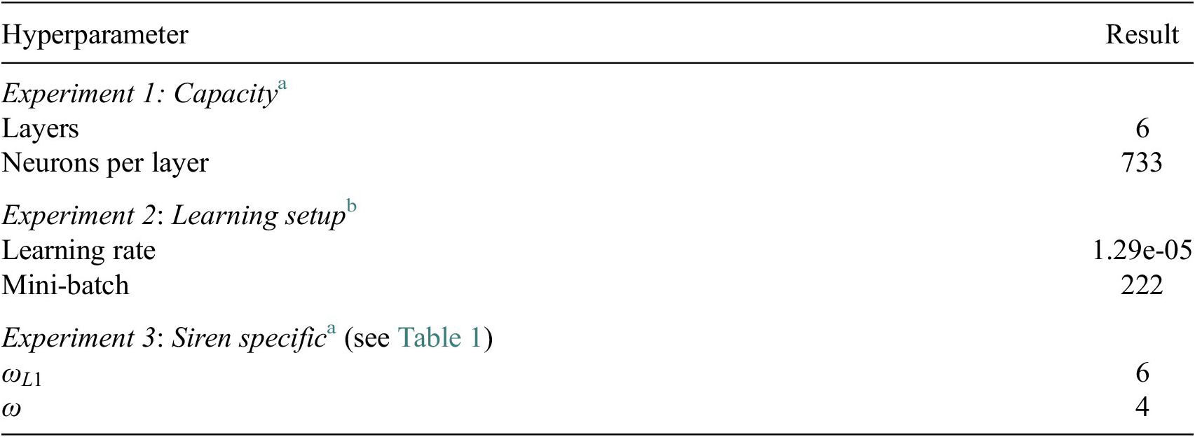
a Bayesian search with maximum learning steps of 10,000.
b Bayesian search and Hyperband early stopping Li et al. (Reference Li, Jamieson, DeSalvo, Rostamizadeh and Talwalkar2018).
In the first of three experiments, we focused on the number of layers and neurons per layer. These parameters showed a strong impact on the functional capacity of the model and thereby the capability of reproducing strongly nonlinear functions.
Our second experiment searched both the learning rate and mini-batch size at the same time. These hyperparameters showed a strong interdependence. To optimize the learning rate and batch size, we used the Hyperband early stopping technique (Li et al., Reference Li, Jamieson, DeSalvo, Rostamizadeh and Talwalkar2018) that allows us to manage which models are promising and should be continued in training, whereas other training runs are stopped. This is of importance, because the learning rate affects the speed of convergence. Stopping after a fixed number of steps would not allow to optimize the learning rate, since a slower convergence could still lead to the lowest metric value.
Finally, a search for the Siren specific parameter $ \omega $
had been conducted by using one parameter for the first layer and another for the perceptrons of the remaining layers. Romero et al. (Reference Romero, Kuzina, Bekkers, Tomczak and Hoogendoorn2022) observed in their experiments that some functions required
$ \omega $
had been conducted by using one parameter for the first layer and another for the perceptrons of the remaining layers. Romero et al. (Reference Romero, Kuzina, Bekkers, Tomczak and Hoogendoorn2022) observed in their experiments that some functions required $ \omega \ge 1,000 $
but most of their experiments led to values
$ \omega \ge 1,000 $
but most of their experiments led to values $ <70 $
. With respect to our data set, the values also had to be selected in an even smaller range
$ <70 $
. With respect to our data set, the values also had to be selected in an even smaller range $ <10 $
in order to be able to map the frequencies well that are inherit in the data.
$ <10 $
in order to be able to map the frequencies well that are inherit in the data.
4.5. One model per calendar month
Neural-SWIFT adopted a one-model-per-calendar-month approach using 12 seasonal data sets (see Section 3.3).
Over the course of a year, the transport represented by the trajectories differs, potentially influencing the ozone tendency within distinct 24-h periods. Consequently, the relationship between input and output parameters exhibits more variability when analyzed over an entire year compared to when it is divided into monthly datasets.
We empirically validated Kreyling et al.’s findings that the monthly models exhibit lower errors when tested against the testing data. One plausible explanation for the observed discrepancy is the seasonal variations in atmospheric flow patterns.
In addition, utilizing a similar design to Polynomial-SWIFT (Kreyling et al., Reference Kreyling, Wohltmann, Lehmann and Rex2018) during the development of Neural-SWIFT enabled a direct comparison of the monthly models between the two methods.
4.6. Extensive training of final model
The configuration comprising the multilayer perceptron architecture, chosen input variables, and hyperparameters (see Table 2) was employed for training until convergence of the cost function could be achieved. Convergence refers to the point at which the training process reaches a stable state, where further iterations do not result in significant improvements in the cost function (see equation (2)). It indicates that the model has learned the underlying patterns and relationships within the data to a satisfactory extent.
The resulting 12 MLPs, one for each month of the year (see Section 3), were used for the simulation runs presented in Section 5.
5. Results
5.1. Neural representation: Neural-SWIFT
The output of the machine learning pipeline is the Neural-SWIFT model, which consists of 12 models (see Section 3.3), one per calendar month. The model uses the MLP architecture shown in Table 2 and employs the choice of input and output variables depicted in Table 3, which according to Figure 6 was the best selection tested.
Selected input and output variables
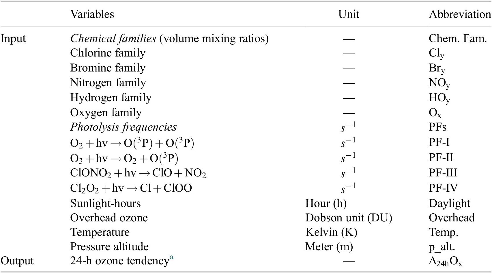
a The point-wise (per air-parcel) 24-h difference in the volume mixing ratio of the Oxygen family: $ {\varDelta}_{24\mathrm{h}}{\mathrm{O}}_{\mathrm{x}}^t={\mathrm{O}}_{\mathrm{x}}^t-{\mathrm{O}}_{\mathrm{x}}^{t-24\mathrm{h}} $
.
$ {\varDelta}_{24\mathrm{h}}{\mathrm{O}}_{\mathrm{x}}^t={\mathrm{O}}_{\mathrm{x}}^t-{\mathrm{O}}_{\mathrm{x}}^{t-24\mathrm{h}} $
.
5.2. Validation in simulation
The validation strategy is a sensitive and important matter in the context of the intended application in climate science. So far, we evaluated each step of the machine learning pipeline (Figure 3) using the cost function (see equation (2)) with respect to the testing data set. From here on, we apply the model in simulation in the ATLAS CTM by replacing the full chemistry module, to compare the results of the full chemistry module with the Neural-SWIFT module. The goal was to achieve a significant speed-up compared to this reference model while achieving comparable accuracy.
Figure 7 depicts a schematic of the application of Neural-SWIFT in ATLAS. For each air parcel (top-left) the 24-h ozone tendency (bottom-right) is calculated point-wise by applying the MLPs of Neural-SWIFT (right).
Schematic of the implementation of Neural-SWIFT in atlas or climate models.

As mentioned in Section 4, not all input variables (e.g., $ {\mathrm{Cl}}_{\mathrm{y}} $
,
$ {\mathrm{Cl}}_{\mathrm{y}} $
, $ {\mathrm{Br}}_{\mathrm{y}} $
,
$ {\mathrm{Br}}_{\mathrm{y}} $
, $ {\mathrm{NO}}_{\mathrm{y}} $
,
$ {\mathrm{NO}}_{\mathrm{y}} $
, $ {\mathrm{HO}}_{\mathrm{y}} $
) are readily available from the model. Some variables need to be calculated, others can be derived from the photolysis table or climatologies of the chemical families. The climatologies are a function of equivalent latitude and altitude. Therefore, equivalent latitude must be calculated to be able to use the climatologies. The calculation of equivalent latitude requires potential vorticity (PV) as a variable. Therefore, if PV is not provided by the climate model, it is necessary for the use of Neural-SWIFT to calculate it in the climate model. Furthermore, the PV is needed for the regime filter for the polar regions to apply the polar SWIFT model and extrapolar Neural-SWIFT model in the correct model domains.
$ {\mathrm{HO}}_{\mathrm{y}} $
) are readily available from the model. Some variables need to be calculated, others can be derived from the photolysis table or climatologies of the chemical families. The climatologies are a function of equivalent latitude and altitude. Therefore, equivalent latitude must be calculated to be able to use the climatologies. The calculation of equivalent latitude requires potential vorticity (PV) as a variable. Therefore, if PV is not provided by the climate model, it is necessary for the use of Neural-SWIFT to calculate it in the climate model. Furthermore, the PV is needed for the regime filter for the polar regions to apply the polar SWIFT model and extrapolar Neural-SWIFT model in the correct model domains.
In contrast to the proposed implementation in climate models, we do not use climatologies in ATLAS, but daily lookup tables from the data set were used when Neural-SWIFT replaced the full chemistry module in ATLAS. This way, the Neural-SWIFT simulation was more comparable to the simulation with the full chemistry module.
In the training process, the input and output variables from the training data were normalized to obtain a distribution with zero mean and unit variance. This step must also be applied in the implementation. Therefore, the mean $ {\mu}_{X^{\mathrm{train}}} $
and standard deviation
$ {\mu}_{X^{\mathrm{train}}} $
and standard deviation $ {\sigma}_{X^{\mathrm{train}}} $
of the complete training data set of all months are used for normalization. Consequently, after calculating the MLP, the regression output
$ {\sigma}_{X^{\mathrm{train}}} $
of the complete training data set of all months are used for normalization. Consequently, after calculating the MLP, the regression output $ {\mathcal{N}}_{\Theta}\left({X}^{\prime}\right) $
must be denormalized by the mean
$ {\mathcal{N}}_{\Theta}\left({X}^{\prime}\right) $
must be denormalized by the mean $ {\mu}_{y^{\mathrm{train}}} $
and the standard deviation
$ {\mu}_{y^{\mathrm{train}}} $
and the standard deviation $ {\sigma}_{y^{\mathrm{train}}} $
.
$ {\sigma}_{y^{\mathrm{train}}} $
.
5.3. Speed-up
Neural-SWIFT shows a computation time faster by orders of magnitude (factor of $ \approx 700 $
faster) compared to the full chemistry module (see Table 4). To enable projections far into the future, the computation time per model day in a climate model is a crucial aspect. Our speed-up meets this fundamental requirement of climate models to perform much faster than real-time.
$ \approx 700 $
faster) compared to the full chemistry module (see Table 4). To enable projections far into the future, the computation time per model day in a climate model is a crucial aspect. Our speed-up meets this fundamental requirement of climate models to perform much faster than real-time.
Computation time

Note. All model runs were coupled to the chemistry and transport model ATLAS and ran on the same server with 48 CPUs, 1.0–3.9 GHz, and 755 GB physical memory. Calculation time refers to chemistry calculation only and does not include time required for transport and mixing in ATLAS.
a The computation time of Polynomial SWIFT also includes the time that was required to detect and handle outliers. For this, Kreyling et al. also used the polynomial approach (domain polynomial) combined with Newton’s method to find a solution in the trained data distribution.
b The Matlab version of ATLAS has been used for comparison.
5.4. Accuracy after 18 month of simulation
An example of the ozone layer resulting from the application of Neural-SWIFT after 18 months of simulation is shown in Figure 8a.
Monthly means (April 2000) of the (a) stratospheric ozone column and (b) zonal mean stratospheric ozone volume mixing ratios are shown after 18-month simulation. The binning used 1° latitude-longitude bins for (a) and zonal means in bins of 1000 m pressure altitude and 5° equivalent latitude for (b). Only the bins in which Neural-SWIFT was applied are shown.

The stratospheric ozone columns of Neural-SWIFT show good agreement to the reference run with relative differences within $ \pm 10\% $
(bottom-right). During the application of Neural-SWIFT, the regions of the polar vortex have been calculated using Polar SWIFT (Wohltmann et al., Reference Wohltmann, Lehmann and Rex2017b).
$ \pm 10\% $
(bottom-right). During the application of Neural-SWIFT, the regions of the polar vortex have been calculated using Polar SWIFT (Wohltmann et al., Reference Wohltmann, Lehmann and Rex2017b).
Figure 8b shows the zonal mean of the volume mixing ratios as a function of pressure altitude and equivalent latitude after 18 months of simulation. Further results showing all 24 months of the simulation can be found in Figures A1–A4 in Appendix A. In general, the figures show a good long-term stability of the results for all pressure altitudes and equivalent latitudes. Regions with higher absolute differences occur where high volume mixing ratios are present and the relative error is small. Furthermore, regions with high relative errors only occur where the volume mixing ratios are very low and the absolute differences are not significant.
5.5. Spatial variability
We were particularly interested in assessing Neural-SWIFT’s capability to replicate the spatial variability at a level similar to the full chemistry module, and over an extended simulation period (two years), given its intended application in climate models.
To evaluate the spatial pattern of variability, we examined the variations in stratospheric ozone columns across different geographic locations throughout a 2-year simulation. We quantified this variability by calculating the standard deviation of the time series at various locations, as depicted in Figure 9.
The figure depicts the spatial pattern of the standard deviation of the time series covering the 2-year simulation period at various locations, measured in du. The binning used 1° latitude–longitude bins. (Top) Our method Neural-SWIFT, (middle) full chemistry module, and (bottom) $ \left[\mathrm{Neural}\hbox{-} \mathrm{SWIFT}\right]-\left[\mathrm{Full}\ \mathrm{chemistry}\right] $
.
$ \left[\mathrm{Neural}\hbox{-} \mathrm{SWIFT}\right]-\left[\mathrm{Full}\ \mathrm{chemistry}\right] $
.

Please note that Figure 9 only displays data within the latitude range of 60° south to 60° north, as the extrapolar Neural-SWIFT model does not simulate ozone in the polar regions (see Section 1.1).
To compare Neural-SWIFT (top) with the full chemistry module (center), we analyzed the differences between them (bottom). Overall, the results are in good agreement with the full chemistry module. However, differences exhibited an increase toward higher latitudes, reaching a maximum absolute difference of $ 9.47 $
DU. Among all the displayed bins,
$ 9.47 $
DU. Among all the displayed bins, $ 75\% $
show absolute differences lower than
$ 75\% $
show absolute differences lower than $ 1.67 $
DU. The Mean Absolute Error (MAE) is
$ 1.67 $
DU. The Mean Absolute Error (MAE) is $ 1.51 $
DU and Root Mean Square Error (RMSE) is
$ 1.51 $
DU and Root Mean Square Error (RMSE) is $ 2.37 $
DU.
$ 2.37 $
DU.
5.6. Error estimation in time series
We also aimed to assess an overall global metric, represented as a single number per day, to measure the quantitative differences over time between the full chemistry module and each of the two methods, polynomial SWIFT (gray) and Neural-SWIFT (black). We conducted a bin-wise comparison of the following variables: (1) the stratospheric ozone column (a function of latitude and longitude), (2) the zonal mean of the ozone volume mixing ratio, and (3) the zonal mean of the 24-h ozone tendency (both a function of pressure altitude and equivalent latitude). For (1), we utilized 1° latitude–longitude bins, while for (2–3), we employed bins based on 1,000 m pressure altitude and 5° equivalent latitude.
The area covered by the spherical coordinates varies with latitude and also with equivalent latitude. We use the following equation (3) to derive the surface area covered by a bin $ \delta A $
that is needed to calculate the weighted mean of the bin-wise absolute differences:
$ \delta A $
that is needed to calculate the weighted mean of the bin-wise absolute differences:
 $$ {\displaystyle \begin{array}{l}\delta A\left(\phi \right)={R}_E^2\delta\ \phi\ \delta \lambda \times \cos \left(\phi \right)\\ {}{A}_{\mathrm{total}}=\sum \limits_{i=1}^{n_{\mathrm{Bins}}}\delta {A}_i\left({\phi}_i\right)\\ {}\hskip-4.5em \mathrm{where}\hskip0.35em {A}_{\mathrm{total}}:\mathrm{surface}\ \mathrm{area}\ \mathrm{of}\;\mathrm{all}\;\mathrm{bins},{R}_E:\mathrm{radius}\ \mathrm{of}\ \mathrm{the}\ \mathrm{Earth},\\ {}\phi, \lambda :\mathrm{latitude}\;\left(\mathrm{or}\ \mathrm{approximation}\ \mathrm{of}\ \mathrm{equivalent}\ \mathrm{latitude}\right)\;\mathrm{and}\ \mathrm{longitude},\\ {}\delta \phi, \delta \lambda :\mathrm{respective}\ \mathrm{spacing}\ \mathrm{used}\ \mathrm{for}\ \mathrm{binning},{n}_{\mathrm{Bins}}:\mathrm{total}\ \mathrm{number}\ \mathrm{of}\ \mathrm{bins}.\end{array}} $$
We use this to calculate the weighted mean of the absolute bin-wise differences ( $ {\mu}_t^{\mathrm{weighted}} $
) for each time-step t.
$ {\mu}_t^{\mathrm{weighted}} $
) for each time-step t.
 $$ {\displaystyle \begin{array}{l}{\mu}_t^{\mathrm{weighted}}\left({B}_t^{\mathcal{N}},{B}_t^{\Phi}\right)=\frac{\sum_{i=1}^{n_{\mathrm{Bins}}}\left(|{B}_{t,i}^{\mathcal{N}}-{B}_{t,i}^{\Phi}|\hskip0.35em \ast \hskip0.35em \delta A({\phi}_i)\right)}{A_{\mathrm{total}}}\\ {}\hskip-4.6em \mathrm{w}\mathrm{h}\mathrm{e}\mathrm{r}\mathrm{e}\hskip0.35em {B}_{t,i}^{\mathcal{N}}:\mathrm{b}\mathrm{i}\mathrm{n}\hskip2pt \mathrm{i}\hskip2pt \mathrm{o}\mathrm{f}\ \mathrm{b}\mathrm{i}\mathrm{n}\mathrm{n}\mathrm{e}\mathrm{d}\ \mathrm{r}\mathrm{e}\mathrm{s}\mathrm{u}\mathrm{l}\mathrm{t}\mathrm{s}\ \mathrm{o}\mathrm{f}\ \mathrm{N}\mathrm{e}\mathrm{u}\mathrm{r}\mathrm{a}\mathrm{l}{\textstyle \hbox{-}}\mathrm{S}\mathrm{W}\mathrm{I}\mathrm{F}\mathrm{T}\ \mathrm{a}\mathrm{t}\ \mathrm{t}\mathrm{i}\mathrm{m}\mathrm{e}\ t,\\ {}{B}_{t,i}^{\Phi}:\mathrm{b}\mathrm{i}\mathrm{n}\hskip2pt \mathrm{i}\hskip2pt \mathrm{o}\mathrm{f}\ \mathrm{b}\mathrm{i}\mathrm{n}\mathrm{n}\mathrm{e}\mathrm{d}\ \mathrm{r}\mathrm{e}\mathrm{s}\mathrm{u}\mathrm{l}\mathrm{t}\mathrm{s}\ \mathrm{o}\mathrm{f}\ \mathrm{t}\mathrm{h}\mathrm{e}\ \mathrm{f}\mathrm{u}\mathrm{l}\mathrm{l}\ \mathrm{c}\mathrm{h}\mathrm{e}\mathrm{m}\mathrm{i}\mathrm{s}\mathrm{t}\mathrm{r}\mathrm{y}\ \mathrm{m}\mathrm{o}\mathrm{d}\mathrm{u}\mathrm{l}\mathrm{e}\ \mathrm{o}\mathrm{f}\ \mathrm{A}\mathrm{T}\mathrm{L}\mathrm{A}\mathrm{S}\ \mathrm{a}\mathrm{t}\ \mathrm{t}\mathrm{i}\mathrm{m}\mathrm{e}\ t,\\ {}\delta A({\phi}_i):\mathrm{s}\mathrm{u}\mathrm{r}\mathrm{f}\mathrm{a}\mathrm{c}\mathrm{e}\ \mathrm{a}\mathrm{r}\mathrm{e}\mathrm{a}\ \mathrm{o}\mathrm{f}\ \mathrm{t}\mathrm{h}\mathrm{a}\mathrm{t}\hskip2pt \mathrm{b}\mathrm{i}\mathrm{n},{A}_{\mathrm{total}}:\mathrm{s}\mathrm{u}\mathrm{r}\mathrm{f}\mathrm{a}\mathrm{c}\mathrm{e}\ \mathrm{a}\mathrm{r}\mathrm{e}\mathrm{a}\ \mathrm{o}\mathrm{f}\hskip2pt \mathrm{a}\mathrm{l}\mathrm{l}\hskip2pt \mathrm{b}\mathrm{i}\mathrm{n}\mathrm{s},{n}_{\mathrm{Bins}}:\mathrm{t}\mathrm{o}\mathrm{t}\mathrm{a}\mathrm{l}\ \mathrm{n}\mathrm{u}\mathrm{m}\mathrm{b}\mathrm{e}\mathrm{r}\ \mathrm{o}\mathrm{f}\ \mathrm{b}\mathrm{i}\mathrm{n}\mathrm{s}.\end{array}} $$
In Figure 10, both Neural-SWIFT and the polynomial approach are evaluated by comparing the results of each of the 2-year simulations with the full chemistry module on a day-by-day basis. The three-time series of the average of the weighted differences in Figure 10a–c show that Neural-SWIFT performs better for the months from July to November than the polynomial approach.
Comparison to polynomial SWIFT. The figure depicts the daily evolution of the mean absolute differences between the full chemistry module and two methods, polynomial SWIFT (gray) and Neural-SWIFT (black). Three variables are presented: (a) stratospheric ozone column, (b) ozone volume mixing ratio, and (c) 24-h ozone tendency. The differences were calculated by initially binning the data (compare Figure 8), using 1° latitude–longitude bins for (a) and 1,000 m of pressure altitude and 5° of equivalent latitude bins for (b) and (c). Subsequently, the daily mean of the absolute differences was calculated, incorporating bin weighting based on surface area (see equation (4)). It is important to note that the mean score does not consider bins within the polar vortex (polar SWIFT module).

Looking at the stratospheric ozone column (Figure 10a), both models provide similar performance in all other months. For the ozone volume mixing ratios and the 24-h ozone tendencies (Figure 10b,c), however, Neural-SWIFT consistently shows a better performance. The error metrics for all three-time series are illustrated in Table 5.
Error metrics of Figure 10

5.7. Time tendency of the differences
Figure 11 shows the global absolute mean error of the 24-h ozone tendency relative to the simulated ozone ( $ {\mathrm{Ox}}_{\mathrm{Full}\ \mathrm{chemistry}} $
) and the global standard deviation of the relative error
$ {\mathrm{Ox}}_{\mathrm{Full}\ \mathrm{chemistry}} $
) and the global standard deviation of the relative error $ {\mathrm{STD}}_{\mathrm{Q}} $
.
$ {\mathrm{STD}}_{\mathrm{Q}} $
. $ {Q}_i $
,
$ {Q}_i $
, $ \overline{Q} $
, and
$ \overline{Q} $
, and $ {\mathrm{STD}}_{\mathrm{Q}} $
are defined by the following equations:
$ {\mathrm{STD}}_{\mathrm{Q}} $
are defined by the following equations:
 $$ {\displaystyle \begin{array}{ll}& {Q}_i=\frac{dOx_{\mathrm{NeuralSWIFT}}^i-{dOx}_{\mathrm{Full}\ \mathrm{chemistry}}^i}{Ox_{\mathrm{Full}\ \mathrm{chemistry}}^i}\\ {}& \overline{Q}=\frac{1}{N}\sum \limits_{i=1}^N\mid {Q}_i\mid \\ {}& {\mathrm{STD}}_Q=\sqrt{\frac{1}{N}\sum \limits_{i=1}^N{\left(|{Q}_i|-\overline{Q}\right)}^2}\\ {}\mathrm{where}& i:\mathrm{individual}\;\mathrm{bin}, dOx:24\hbox{-} \mathrm{hour}\ \mathrm{ozone}\ \mathrm{tendency},\\ {}& Ox:\mathrm{ozone}\ \mathrm{volume}\ \mathrm{mixing}\ \mathrm{ratio},\hskip0.35em N:\mathrm{number}\ \mathrm{of}\ \mathrm{bins}\end{array}}. $$
The time evolution employing error-Q (black line) and the std dev (gray) was calculated as defined in equation (5). The binning used 1,000 m pressure altitude and 5° equivalent latitude). A weighting of the bins according to their surface area (equation (4)) was performed. Bins of the polar vortex (polar SWIFT module) are not included in the mean score.

The equations are based on bin-wise differences according to Kreyling et al. (Reference Kreyling, Wohltmann, Lehmann and Rex2018). Bins with values of $ {Ox}_{\mathrm{Full}\ \mathrm{chemistry}} $
below 100 ppb were removed to avoid spurious large errors when the absolute values are low. This affects less than 10% of the data.
$ {Ox}_{\mathrm{Full}\ \mathrm{chemistry}} $
below 100 ppb were removed to avoid spurious large errors when the absolute values are low. This affects less than 10% of the data.
The daily mean $ \overline{Q} $
of the relative error
$ \overline{Q} $
of the relative error $ {Q}_i $
remained close to zero throughout the simulation. Over the entire simulation period, the MAE is found to be
$ {Q}_i $
remained close to zero throughout the simulation. Over the entire simulation period, the MAE is found to be $ 0.31\frac{\%}{\mathrm{day}} $
, and the RMSE is
$ 0.31\frac{\%}{\mathrm{day}} $
, and the RMSE is $ 0.33\frac{\%}{\mathrm{day}} $
. The fall season showed the largest relative error (max
$ 0.33\frac{\%}{\mathrm{day}} $
. The fall season showed the largest relative error (max $ \overline{Q} $
of
$ \overline{Q} $
of $ 0.68\frac{\%}{\mathrm{day}} $
and max
$ 0.68\frac{\%}{\mathrm{day}} $
and max $ {\mathrm{STD}}_{\mathrm{Q}} $
of
$ {\mathrm{STD}}_{\mathrm{Q}} $
of $ 7.31\frac{\%}{\mathrm{day}} $
). After this perturbation, however, the ozone tendencies were again estimated very accurately (see Figure 11).
$ 7.31\frac{\%}{\mathrm{day}} $
). After this perturbation, however, the ozone tendencies were again estimated very accurately (see Figure 11).
As seen in Figure 11, the differences to the full chemistry do not exhibit significant growth over time. This emphasizes that these error scores should not be interpreted as a systematic error that would lead to a substantial increase in error as the simulation progresses.
The result that Neural-SWIFT achieves a high accuracy (small differences over time) and therefore allows for a stable simulation can also be confirmed by Figure 12, which shows the zonal mean values (equivalent latitude) of stratospheric ozone columns over time. Only the equivalent latitude range between 60° S and 60° N is shown, since the extrapolar Neural SWIFT model does not simulate ozone in the polar regions. The results of the simulation demonstrate a good agreement with the reference model (ATLAS) for various seasons in both hemispheres. Approximately 75% of the bins show differences of only $ \pm 5 $
DU (white color). Over the 2-year simulation period, the MAE is found to be
$ \pm 5 $
DU (white color). Over the 2-year simulation period, the MAE is found to be $ 3.65 $
DU, and the RMSE is
$ 3.65 $
DU, and the RMSE is $ 4.70 $
DU. These error metrics indicate an improvement of
$ 4.70 $
DU. These error metrics indicate an improvement of $ >11\% $
over Polynomial SWIFT (see Figure B1 in Appendix B).
$ >11\% $
over Polynomial SWIFT (see Figure B1 in Appendix B).
(First row) Shown are zonal mean values (Binning: 3° equivalent latitude) of stratospheric ozone columns in Dobson Units (DU) over time of the results of a 2-year simulation using the novel artificial neural networks of Neural-SWIFT. The areas which also covered the polar vortex were removed and are shown in gray. The results are evaluated by difference plots (comparing to a simulation run that used the full chemistry module of ATLAS): (second row) $ \left[\mathrm{Neural}\hbox{-} \mathrm{SWIFT}\right]-\left[\mathrm{Full}\ \mathrm{chemistry}\right] $
and (third row)
$ \left[\mathrm{Neural}\hbox{-} \mathrm{SWIFT}\right]-\left[\mathrm{Full}\ \mathrm{chemistry}\right] $
and (third row) $ \frac{\left[\mathrm{Neural}\hbox{-} \mathrm{SWIFT}\right]-\left[\mathrm{Full}\ \mathrm{chemistry}\right]}{\left[\mathrm{Full}\ \mathrm{chemistry}\right]} $
.
$ \frac{\left[\mathrm{Neural}\hbox{-} \mathrm{SWIFT}\right]-\left[\mathrm{Full}\ \mathrm{chemistry}\right]}{\left[\mathrm{Full}\ \mathrm{chemistry}\right]} $
.

5.8. Implementation into climate models
Neural SWIFT operates point-wise on the grid points of the climate model, is inherently mesh-free, and can thereby handle different grid resolutions. The choice of input variables was also made in such a way that it is possible to calculate them for the grid points.
Some input parameters of our model (e.g., $ {\mathrm{Cl}}_{\mathrm{y}} $
,
$ {\mathrm{Cl}}_{\mathrm{y}} $
, $ {\mathrm{Br}}_{\mathrm{y}} $
,
$ {\mathrm{Br}}_{\mathrm{y}} $
, $ {\mathrm{NO}}_{\mathrm{y}} $
,
$ {\mathrm{NO}}_{\mathrm{y}} $
, $ {\mathrm{HO}}_{\mathrm{y}} $
) are generally not available in climate models like ICON (Rieger et al., Reference Rieger, Bangert, Bischoff-Gauss, Förstner, Lundgren, Reinert, Schröter, Vogel, Zängl, Ruhnke and Vogel2015; Schröter et al., Reference Schröter, Rieger, Stassen, Vogel, Weimer, Werchner, Förstner, Prill, Reinert, Zängl, Giorgetta, Ruhnke, Vogel and Braesicke2018). To produce the training data of Neural-SWIFT for any grid point, these variables were calculated from the chemical species of the full chemistry model. For the application in a climate model, monthly climatologies of the volume mixing ratios of the chemical families interpolated to the model time of the climate model have to be used (see Section 5).
$ {\mathrm{HO}}_{\mathrm{y}} $
) are generally not available in climate models like ICON (Rieger et al., Reference Rieger, Bangert, Bischoff-Gauss, Förstner, Lundgren, Reinert, Schröter, Vogel, Zängl, Ruhnke and Vogel2015; Schröter et al., Reference Schröter, Rieger, Stassen, Vogel, Weimer, Werchner, Förstner, Prill, Reinert, Zängl, Giorgetta, Ruhnke, Vogel and Braesicke2018). To produce the training data of Neural-SWIFT for any grid point, these variables were calculated from the chemical species of the full chemistry model. For the application in a climate model, monthly climatologies of the volume mixing ratios of the chemical families interpolated to the model time of the climate model have to be used (see Section 5).
The variables of the photolysis frequencies can be taken from a photolysis table when implemented in a climate model (see Section 4).
Some variables such as the solar zenith angle, the overhead ozone column, or the sunlight hours may not be readily available by the climate model, but can be calculated in the model.
To couple Neural-SWIFT to climate models, it was required to translate the neural network model from the programming language of the development framework (PyTorch Lightning Falcon, Reference Falcon2019 (Python)) to the programming language of the application framework. The multilayer perceptron of Neural-SWIFT can be expressed by the adjustable neural network parameters (weights and biases) $ \Theta $
. After training the model, we stored the raw weight matrices and bias vectors of each layer and translated the Python code to a vectorized version in other programming languages. Neural-SWIFT is already translated from Python to Matlab (process model ATLAS) and also Fortran, which enables the application in climate models like ICON.
$ \Theta $
. After training the model, we stored the raw weight matrices and bias vectors of each layer and translated the Python code to a vectorized version in other programming languages. Neural-SWIFT is already translated from Python to Matlab (process model ATLAS) and also Fortran, which enables the application in climate models like ICON.
6. Conclusions
In climate modeling, the stratospheric ozone layer is typically only considered in a highly simplified form due to computational constraints. For climate projections, it would be of advantage to include the mutual interactions between stratospheric ozone, temperature, and atmospheric dynamics to accurately represent radiative forcing.
The overarching goal of our research is to replace the ozone chemistry in climate models with a machine-learned neural representation of the stratospheric ozone chemistry that allows for a fast, but accurate and stable simulation.
We explored whether a neural representation of the stratospheric ozone chemistry is well suited to represent the model formulation of the ATLAS Chemistry and Transport Model. We used a training data set derived from a simulation run of ATLAS that used the full chemistry scheme to explore correlations between the possible input variables of the neural network and the target variable (24-h tendency of ozone) and to develop and train the neural network model of ozone chemistry (called Neural-SWIFT). We analyzed different variants of multilayer perceptrons convenient for physical problems to learn a neural representation of the regression task. We performed a comprehensive hyperparameter optimization of the multilayer perceptron using Bayesian search and Hyperband early stopping. We validated our model by implementing it in the Chemistry and Transport Model (CTM) ATLAS and comparing computation time, accuracy, and stability with the full chemistry module.
We performed a benchmark by comparing the differences between Neural-SWIFT and the polynomial approach of SWIFT with the full chemistry module. The neural representations showed good agreement with the full stratospheric chemistry model during a 2-year long simulation. Chemical production and loss, as well as seasonality in both hemispheres, was well represented by Neural-SWIFT. The time evolution of the errors showed that a stable long-term simulation of a complex process like atmospheric ozone chemistry is feasible. Our model had a computation time that was a factor of 700 faster than the full chemistry module. Neural-SWIFT’s accuracy during a 2-year simulation run outperforms SWIFT’s previous polynomial approach in terms of all applied metrics, this despite the former polynomial approach of SWIFT also applied a method to detect and handle outliers.
Future advances in climate science related to robustness, accuracy, and computation time of simulations can benefit significantly from interdisciplinary research incorporating data science and machine learning methodology. We see great potential in the developing research on digital twins for climate system processes, such as Neural-SWIFT, that can serve as AI surrogate models in climate simulations. It is expected that numerical models will more often blend conventional algorithms with deep learning solutions (Bauer et al., Reference Bauer, Dueben, Hoefler, Quintino, Schulthess and Wedi2021a, Reference Bauer, Stevens and Hazeleger2021b; Irrgang et al., Reference Irrgang, Boers, Sonnewald, Barnes, Kadow, Staneva and Saynisch-Wagner2021) and just as Neural-SWIFT already does, also benefit from the advantages offered by modern high-performance computers that support parallel processing, including support for parallel processing using GPUs.
A challenge arises from the limited generalizability of modeled processes beyond the scope of the included environmental conditions. Data-driven models, despite their ability to learn patterns directly from data, struggle to extrapolate beyond the range of observed conditions due to limitations in the training data. The next step toward a robust application of Neural-SWIFT is to know when Neural-SWIFT is forced to extrapolate. Different techniques are possible to measure extrapolation. One technique that has been used by the previous polynomial approach of SWIFT is to focus on the training data distribution. In regions of the hyper-dimensional space, where less dense or no data points exist an extrapolation of the model is likely. Another method that we want to focus on in the future is the employment of the model uncertainty to detect an application that is out-of-distribution with respect to the training data. A promising strategy called “Deep Ensembles” (Lakshminarayanan et al., Reference Lakshminarayanan, Pritzel and Blundell2017) employs several multilayer perceptrons as an ensemble. This strategy can be implemented using exactly the methodology of Neural-SWIFT and can be used to detect extrapolation. One possibility to ensure that Neural-SWIFT always interpolates in a future version is by employing the full chemistry model whenever we encounter a grid point outside the training distribution. The obtained results can then be used and stored for additional training, gradually expanding the trained range over time. This approach can be implemented as an active learning technique, utilizing the model’s uncertainty to determine which regions require retraining.
In this way, climate simulations can benefit from an interactive, fast, and highly accurate representation of stratospheric ozone chemistry that is always aware of its uncertainty and thus its reliability.
Acknowledgments
The authors gratefully acknowledge the Earth System Modelling Project (ESM) for funding this work by providing computing time on the ESM partition of the supercomputer JUWELS at the Jülich Supercomputing Centre (JSC). The results shown here use both the Python and Matlab versions of Neural-SWIFT, but future applications in climate models such as ICON can rely on the translation to Fortran, which was gratefully implemented by Andrey Vlasenko from Hereon (Geesthacht). We thank ECMWF for providing reanalysis data.
Author contribution
Conceptualization: M.R., P.M., I.W., R.L., D.K., H.M.; Data curation: I.W., H.M., D.K.; Data visualization/Formal analysis: H.M.; Investigation/Methodology: H.M.; Software: D.K., H.M. (SWIFT Interface for ATLAS); H.M. (Neural-SWIFT); Writing—original draft: H.M. All authors approved the final submitted draft.
Competing interest
The authors declare none.
Data availability statement
This research adheres to the FAIR guiding principles (Wilkinson et al., Reference Wilkinson, Dumontier, Aalbersberg, Appleton, Axton, Baak, Blomberg, Boiten, da Silva Santos, Bourne, Bouwman, Brookes, Clark, Crosas, Dillo, Dumon, Edmunds, Evelo, Finkers, Gonzalez-Beltran, Gray, Groth, Goble, Grethe, Heringa, ’t Hoen, Hooft, Kuhn, Kok, Kok, Lusher, Martone, Mons, Packer, Persson, Rocca-Serra, Roos, van Schaik, Sansone, Schultes, Sengstag, Slater, Strawn, Swertz, Thompson, van der Lei, van Mulligen, Velterop, Waagmeester, Wittenburg, Wolstencroft, Zhao and Mons2016) to ensure the data’s reusability and the reproducibility of our presented results. The input and output data pairs used in this study are both Findable and Accessible through the open-access library PANGAEA (Mohn et al., Reference Mohn, Kreyling, Wohltmann, Lehmann and Rex2021). To promote Interoperability and Reusability, we have provided vanilla code on GitHub that utilizes this benchmark dataset and the Neural-SWIFT method. The code can be accessed at the following link: https://doi.org/10.5281/zenodo.7388368.
Ethics statement
The research meets all ethical guidelines, including adherence to the legal requirements of the study country.
Funding statement
H.M. was supported by grants from the Helmholtz School for Marine Data Science (MarDATA) (HIDSS-0005). H.M. acknowledges support by the Open Access Publication Funds of Alfred-Wegener-Institut Helmholtz-Zentrum für Polar- und Meeresforschung.
A. Appendix A: Simulation results of Neural-SWIFT
A.1. Monthly zonal means
Two 24-month long (January 1999–December 2001) simulation runs were performed in the ATLAS CTM using either the AI surrogate model Neural-SWIFT (first column) or the full chemistry module (second column).
The first two columns depict the monthly zonal means of the stratospheric ozone volume mixing ratio (parts per million) with Neural-SWIFT in the first column and the full chemistry scheme in the second column. The differences between both runs are depicted in the third column followed by the relative differences in the fourth column.
The binning used zonal means over 1000 m pressure altitude (vertical) and 5° equivalent latitude (horizontal). Bins that contained air masses from outside the regime of Neural-SWIFT or that would represent a mixture of air parcels from the polar SWIFT module and Neural-SWIFT are not shown.
Monthly zonal mean stratospheric ozone volume mixing ratios (parts per million) from January to June 1999 are shown.

Monthly zonal mean stratospheric ozone volume mixing ratios (parts per million) from July to December 1999 are shown.

Monthly zonal mean stratospheric ozone volume mixing ratios (parts per million) from January to June 2000 are shown.

Monthly zonal mean stratospheric ozone volume mixing ratios (parts per million) from July to December 2000 are shown.

B. Appendix B: Simulation results of the previous polynomial approach of SWIFT
(First row) Shown are zonal mean values (Binning: 3° equivalent latitude) of stratospheric ozone columns in Dobson Units (DU) over time of the results of a 2-year simulation using the previous polynomial approach of SWIFT. The areas which also covered the polar vortex were removed and are shown in gray. The results are evaluated by difference plots (comparing to a simulation run that used the full chemistry module of ATLAS):(second row) $ \left[\mathrm{Polynomial}\ \ \mathrm{SWIFT}\right]-\left[\mathrm{Full}\ \mathrm{chemistry}\right] $
and (third row)
$ \left[\mathrm{Polynomial}\ \ \mathrm{SWIFT}\right]-\left[\mathrm{Full}\ \mathrm{chemistry}\right] $
and (third row) $ \frac{\left[\mathrm{Polynomial}\ \ \mathrm{SWIFT}\right]-\left[\mathrm{Full}\ \ \mathrm{chemistry}\right]}{\left[\mathrm{Full}\ \mathrm{chemistry}\right]}. $

C. Appendix C: Hyperparameter optimization
C.1. Hyperparameter optimization: Capacity
Search for the number of layers and number of neurons per layer. The color scale shows the result of the cost function with respect to the normalized testing data.

C.2. Hyperparameter optimization: Learning setup
Learning rate and mini-batch size.

C.3. Hyperparameter optimization: Siren specific
Siren specific (see Table 1): omega first and other layers.

D. Appendix D: Acronyms and glossary
D.1. Acronyms
- ANNs:
-
artificial neural networks
- ATLAS:
-
Alfred Wegener InsTitute LAgrangian Chemistry/Transport System
- CCMs:
-
Chemistry Climate Models
- CHEM2D-OPP:
-
CHEM2D-Ozone Photochemistry Parameterization
- CTM:
-
Chemistry and Transport Model
- DU:
-
Dobson Units
- ECMWF:
-
European Centre of Medium-Range Weather Forecasts
- GCM:
-
General Circulation Model
- GPU:
-
graphics processing unit
- Linoz:
-
linearized ozone
- MAE:
-
mean absolute error
- MLP:
-
multilayer perceptron
- MSE:
-
mean squared error
- NDF:
-
numerical differentiation formulas
- ppb:
-
parts per billion
- PV:
-
potential vorticity
- ReLU:
-
rectified linear unit
- RMSE:
-
root mean square error
- SWIFT:
-
Semi-empirical Weighted Iterative Fit Technique
- VMR:
-
volume mixing ratio
- WACCM:
-
Whole Atmosphere Community Climate Model
D.2. Glossary
- Air parcel:
-
An air parcel is a small imaginary volume of air consisting of ever the same molecules used to describe basic concepts of atmospheric physics and to define atmospheric variables like temperature or mixing ratios as scalar fields of location and time. The air parcel needs to be large enough to contain a sufficient number of molecules for the concepts of thermodynamics to apply (to be able to define thermodynamic quantities like pressure), but small enough to be able to define these variables as continuous scalar fields of location and time.
- Baseline (ReLU):
-
A reference model used to compare different architectures of multilayer perceptrons applying the ReLU activation function.
- Bayesian search:
-
Unlike random or grid search, Bayesian search stores past evaluation results and, with the help of a probabilistic model, uses them to select a new set of hyperparameters that have a high probability of reducing the model inaccuracy.
- Bromine family:
-
$ {\mathrm{Br}}_y=\mathrm{Br}+2\times {\mathrm{Br}}_2+\mathrm{BrCl}+\mathrm{BrO}+\mathrm{HBr}+\mathrm{HOBr}+{\mathrm{Br}\mathrm{ONO}}_2. $
- Chemical families:
-
A chemical family describes a collection of short-lived chemical species that quickly transform into each other by fast reactions, but where the sum of the species has a much longer chemical lifetime.
- Chemistry and Transport Model:
-
A chemistry and transport model is a global numerical atmospheric model used to model the chemistry, transport, and mixing of species in the atmosphere. In contrast to a CCM (chemistry climate model) or GCM (general circulation model), it does not contain a dynamical core. Instead, meteorological fields like wind, temperature, and pressure are taken from an external source.
- Chlorine family:
-
$ {\mathrm{Cl}}_y=\mathrm{Cl}+2\times {\mathrm{Cl}}_2+\mathrm{ClO}+\mathrm{OClO}+2\times {\mathrm{Cl}}_2{\mathrm{O}}_2+\mathrm{HCl}+\mathrm{HOCl}+{\mathrm{Cl}\mathrm{ONO}}_2+{\mathrm{Cl}\mathrm{NO}}_2+\mathrm{BrCl}. $
- Equivalent latitude:
-
Similar to the geographic latitude the equivalent latitude can be employed as a coordinate that is often used in atmospheric science. The equivalent latitude of a PV contour is defined as the latitude that a circle centered on the pole and enclosing the same area as the given PV contour would have.
$ \mathrm{eq}.\mathrm{latitude}={\sin}^{-1}\frac{1-A\left({\mathrm{PV}}_{\mathrm{max}},\Theta \right)}{2\times \mathrm{pi}\times {R}_E^2} $
, where
$ A\left({\mathrm{PV}}_{\mathrm{max}},\Theta \right) $
: area up to a max potential vorticity on an isentropic surface with potential temperature
$ \Theta $
,
$ {R}_E=6,371,000\;\mathrm{m} $
: Earth radius. - Hydrogen family:
-
$ {\mathrm{H}\mathrm{O}}_y={\mathrm{H}}_2\mathrm{O}. $
- Hyperband:
-
Hyperband early stopping (Li et al., Reference Li, Jamieson, DeSalvo, Rostamizadeh and Talwalkar2018) helps to identify a promising set of hyperparameters. This method continues to train only the best-performing runs and stops runs that are not promising with respect to reducing the model accuracy and reducing GPU hours.
- Latent function:
-
Describes the hidden and in many applications not beforehand known function. In our case, the underlying function is not unknown, since it is based on the computationally expensive solution of a complex system of differential equations over 24 h.
- Nitrogen family:
-
$ {\mathrm{N}\mathrm{O}}_y=\mathrm{NO}+{\mathrm{N}\mathrm{O}}_2+{\mathrm{N}\mathrm{O}}_3+2\times {\mathrm{N}}_2{\mathrm{O}}_5+{\mathrm{HNO}}_3+{\mathrm{HO}}_2{\mathrm{N}\mathrm{O}}_2+\mathrm{N}+{\mathrm{ClONO}}_2+{\mathrm{ClNO}}_2+{\mathrm{BrONO}}_2. $
- Oxygen family:
-
Family of “odd oxygen”
$ {\mathrm{O}}_x={\mathrm{O}}_3+\mathrm{O}+{\mathrm{O}}_{1\mathrm{D}}. $
- Polar vortex:
-
Refers to a long-lived and rotating low-pressure area of large extent that occurs mainly at the north or south pole in the stratosphere in a given winter. It is surrounded by a band of strong, counterclockwise air currents, the vortex, which reduces the exchange of air with other air masses and thus allows very cold temperatures during the polar night.
- Prescribed ozone fields:
-
A noninteractive representation of ozone concentrations often implemented via daily or monthly averaged three- or two-dimensional look-up tables.
- Pressure altitude:
-
We use the log-pressure height in the following form:
$ z(p)=-H\times \log \left(\frac{p}{p_0}\right) $
, where
$ H $
, scale height in m;
$ p $
, pressure;
$ {p}_0=1,000\;\mathrm{hPa} $
: Reference pressure.


 Open access