


1. Introduction
Vortex rings are prevalent flow phenomena present both as independent entities and within more intricate flow systems. Ranging from basic smoke rings generated by a pipe-tobacco enthusiast (Fairholt Reference Fairholt1876) to intricate fuel injection processes (Sazhin et al. Reference Sazhin, Kaplanski, Feng, Heikal and Bowen2001; Begg et al. Reference Begg, Kaplanski, Sazhin, Hindle and Heikal2009; Wu et al. Reference Wu, Zhang, Zhang, Guo, Zhang and Gao2020), they have consistently captivated researchers and motivated extensive investigation (Fuentes Reference Fuentes2014). Furthermore, interactions between vortices and their surrounding surfaces share that ubiquity (Smith, Walker & Doligaski Reference Smith, Walker and Doligaski1994). In nature, vortex–surface interactions are evident in phenomena such as left ventricular flows (Pierrakos & Vlachos Reference Pierrakos and Vlachos2006; Okafor et al. Reference Okafor, Raghav, Condado, Midha, Kumar and Yoganathan2017), unsteady flows through fish cage arrays (Klebert et al. Reference Klebert, Lader, Gansel and Oppedal2013) and the dynamics of coughs on protective barriers (McAtee et al. Reference McAtee, Morris, Shah and Raghav2021), among others. In engineering applications, such interactions are common in energy harvesting using flexible underwater cantilevers (Peterson & Porfiri Reference Peterson and Porfiri2012), heat transfer of impinging jets for cooling applications (Jabbar & Naguib Reference Jabbar and Naguib2019), and in fluid dynamic applications as with the interaction between a leading edge vortex sheet and its wall-generated vorticity on a plunging flat plate (Panah, Akkala & Buchholz Reference Panah, Akkala and Buchholz2015). These complicated vortex–wall interactions are often analysed by simplifying the problem into the canonical vortex ring–wall collision, modelling unsteady fluid–structure interactions with high control and repeatability (Jabbar & Naguib Reference Jabbar and Naguib2019).
The comprehension of vortex ring formation and evolution is crucial for their application in studies. Luckily, this subject is well documented (Wood Reference Wood1901; Maxworthy Reference Maxworthy1972; Didden Reference Didden1979; Glezer Reference Glezer1988; Weigand & Gharib Reference Weigand and Gharib1997; Mohseni, Ran & Colonius Reference Mohseni, Ran and Colonius2001; Raphaël & Jovan Reference Raphaël and Jovan2021). When fluid exits an orifice, the boundary layer rolls into a vortex core. The continued roll-up creates dense vortex lines, leading to a self-induced axial velocity. Once this self-induced velocity exceeds the shear layer velocity that feeds the core, the vortex detaches (‘pinches off’) and advects at its self-induced velocity, with a trailing jet following close behind. If the bulk flow stops before core saturation, a stable vortex ring without a trailing jet forms. Gharib, Rambod & Shariff (Reference Gharib, Rambod and Shariff1998) proposed a universal time scale for vortex ring creation, with a critical time $U_{\!p} t/ D \approx 4$
marking the circulation limit of the vortex ring, where
$U_{\!p} t/ D \approx 4$
marking the circulation limit of the vortex ring, where $U_{\!p}$
is the velocity of the piston,
$U_{\!p}$
is the velocity of the piston, $t$
is the time and
$t$
is the time and $D$
is the diameter of the nozzle. Many have since suggested variant formation numbers for different conditions (Dabiri & Gharib Reference Dabiri and Gharib2004; Krueger, Dabiri & Gharib Reference Krueger, Dabiri and Gharib2006; Afanasyev Reference Afanasyev2006; Pedrizzetti Reference Pedrizzetti2010; Domenichini Reference Domenichini2011; Sattari et al. Reference Sattari, Rival, Martinuzzi and Tropea2012). Dabiri (Reference Dabiri2009) introduced a formation time coefficient to address different constraints, suggesting that although the critical formation number is not universally fixed, it remains a central concept in vortex ring formation.
$D$
is the diameter of the nozzle. Many have since suggested variant formation numbers for different conditions (Dabiri & Gharib Reference Dabiri and Gharib2004; Krueger, Dabiri & Gharib Reference Krueger, Dabiri and Gharib2006; Afanasyev Reference Afanasyev2006; Pedrizzetti Reference Pedrizzetti2010; Domenichini Reference Domenichini2011; Sattari et al. Reference Sattari, Rival, Martinuzzi and Tropea2012). Dabiri (Reference Dabiri2009) introduced a formation time coefficient to address different constraints, suggesting that although the critical formation number is not universally fixed, it remains a central concept in vortex ring formation.
The focal topic of this study is the dynamics of the vortex ring–wall interaction, a well-documented process in the scientific literature (Boldes & Ferreri Reference Boldes and Ferreri1973; Yamada et al. Reference Yamada, Kohsaka, Yamabe and Matsui1982; Cerra & Smith Reference Cerra and Smith1983; Lim, Nickels & Chong Reference Lim, Nickels and Chong1991; Green Reference Green1995). In the classical interaction scenario between a vortex ring and a wall, a travelling vortex ring, known as the primary vortex ring (PVR), encounters its mirror image at the wall. Inviscid analysis predicts that the PVR decelerates as it approaches the wall and extends asymptotically radially due to the influence of its image (Walker et al. Reference Walker, Smith, Cerra and Doligalski1987). Introducing a no-slip boundary condition at the interaction surface creates a boundary layer, which generates vorticity opposite to that of the PVR. As the PVR extends along the wall, this boundary layer experiences an adverse pressure gradient, as elaborated by Matsui, Mochizuki & Yamabe (Reference Matsui, Mochizuki and Yamabe1985), Chu et al. (Reference Chu, Wang, Chang, Chang and Chang1995 b) and Naguib & Koochesfahani (Reference Naguib and Koochesfahani2004). If the Reynolds number is sufficiently high, the boundary layer may detach and coalesce into a cohesive secondary vortex ring (SVR). Mutual induction between the primary and secondary structures induces an orbital motion away from the wall, termed vortex rebound. Initially, viscous diffusion within the vortex core has minimal impact (Saffman Reference Saffman1970), but pronounced vorticity gradients resulting from close proximity to the core enhance vorticity diffusion (Ogami & Akamatsu Reference Ogami and Akamatsu1991). Being a linear mechanism, diffusion causes vorticity cancellation between cores, leading to a rapid reduction in each core circulation, known as cross-core cancellation. Vortex rings at higher Reynolds numbers, due to greater inertia, are more resilient to core diffusion and repeat the rebound, forming a tertiary vortex ring (TVR) of opposite sign. The increased instabilities in the vortex structures prevent the coherent development of the flow field beyond this point.
Truly infinite boundaries exist only in theoretical discussion. The examples from the introduction earlier have spurred investigations into the interaction dynamics between vortex rings and atypical walls. In studies of vortex rings colliding with inclined walls, surface inclination significantly influences the collision (Lim Reference Lim1989; Verzicco & Orlandi Reference Verzicco and Orlandi1994; Cheng, Lou & Luo Reference Cheng, Lou and Luo2010; Couch & Krueger Reference Couch and Krueger2011). Asymmetrical vortex stretching and dissipation of the PVR emerge as critical forces, creating circumferential vorticity and pressure gradients that drive boundary-layer fluid from one vortex core to another. Geometry alone notably alters rebound and flow evolution. In particular, Couch & Krueger (Reference Couch and Krueger2011) identified that the rebound ejection angle of the flow correlates with surface-induced vorticity. Other research has examined interactions with porous walls (Adhikari & Lim Reference Adhikari and Lim2009; Naaktgeboren, Krueger & Lage Reference Naaktgeboren, Krueger and Lage2012; Hyrnuk, Van Luipen & Bohl Reference Hyrnuk, Van Luipen and Bohl2012), showing that porosity and Reynolds number play a vital role in flow field evolution. The porous surface’s unique flow features alter the rebound trajectory of the PVR (Naaktgeboren et al. Reference Naaktgeboren, Krueger and Lage2012). Moreover, researchers have studied vortex interactions with non-flat surfaces, albeit in the form of vortex sheets rather than rings. Morris & Williamson (Reference Morris and Williamson2020) found that wavy walls modify secondary vorticity generation, accelerating primary vortex sheet dissipation. Investigations of vortex rings with various sized cylinders (New & Zang Reference New and Zang2017) show that surface curvature profoundly affects the development of secondary vorticity and the overall flow field. The interaction of vortex rings with a concave hemisphere was explored by Ahmed & Erath (Reference Ahmed and Erath2023), revealing how spatial constraints limit vortex stretching and in some cases how edge-generated vorticity can significantly alter the flow. Similarly, New, Xu & Shi (Reference New, Xu and Shi2024) analysed vortex ring interactions with a convex hemisphere, highlighting the geometric influence on vortex structures, trajectories, velocities and circulation. In summary, it is well recognised that surface shape and curvature and, at times, Reynolds number significantly affect vortex ring–wall interaction dynamics, sometimes leading to paradigm shifts in PVR rebound behaviour.
In light of the intricate vortex ring–wall interactions for different geometries, it is valuable to separate the impact of limited extent from that of specific shapes or curvatures. To that end, this study investigates the finite-wall effects in the classical interaction between a vortex ring and a flat wall. Prior research primarily covers two-dimensional vortex dipole–wall interactions, largely via numerical methods. Peterson & Porfiri (Reference Peterson and Porfiri2013) examined the interaction between a vortex dipole and a semi-infinite flat plate coinciding with the centre of the dipole, finding an increased secondary vorticity at the edge of the plate. This enhanced secondary vorticity caused prolonged mutual induction orbits between the PVR and SVR. Therefore, higher Reynolds numbers were required for the vortex rebound to recur and form tertiary structures. Zivkov, Peterson & Yarusevych (Reference Zivkov, Peterson and Yarusevych2017) expanded this to flexible plates, noting that surface deformation yields less secondary circulation than rigid cases, but more than infinite ones. At lower Reynolds numbers, this altered trajectory results in multiple vortex rebound events, crucial for energy harvesting applications. Furthermore, Danaila (Reference Danaila2004) studied vortex dipole interactions with cubic surface obstacles, the closest analogue to the current work, revealing that smaller wall sizes enhanced secondary vorticity by prompting earlier secondary vorticity roll-up. The varying primary–secondary circulation ratios influenced vortex trajectories and flow field evolution. To the best knowledge of the authors, there is yet no work, experimental or numerical, isolating the finite-wall effects in the classical vortex ring–wall interaction.
Researchers studying these vortex ring–wall interactions have consistently used flow visualisation and flow field measurements to study this problem under various conditions. Typically, the analysis of macro-structures such as PVR, SVR and TVR involves examining their formation and evolution, identifying how they differ from the classic flat plate problem and other geometries in the study (Adhikari & Lim Reference Adhikari and Lim2009; Couch & Krueger Reference Couch and Krueger2011; Hyrnuk et al. Reference Hyrnuk, Van Luipen and Bohl2012; New & Zang Reference New and Zang2017; New et al. Reference New, Long, Zang and Shi2020; Ahmed & Erath Reference Ahmed and Erath2023). Some studies track the core locations over time to compare trajectories and also report vortex circulation evolution. As a result of these analyses, researchers are able to describe how the surface geometry significantly affects flow field evolution in vortex ring–wall collisions. The secondary vorticity’s development varies with wall characteristics, impacting the strength of rolled-up vortices, which then influences rebound characteristics. The vortex trajectory is controlled by the circulation ratio between primary and secondary vortices, with stronger secondary vortices causing larger curvature rebound orbits. Research on two-dimensional finite-wall interactions indicates that the limited surface extent significantly influences flow field dynamics (Danaila Reference Danaila2004; Peterson & Porfiri Reference Peterson and Porfiri2012), but further analysis of the physical mechanisms is needed, especially for flat, infinite surfaces where vortex stretching in three dimensions is missing from the two-dimensional vortex impingement.
Surface plate shape is known to strongly influence vortex ring–wall interactions, modifying secondary vorticity, rebound trajectories and ejection angles, with some studies even reporting Reynolds number dependence. Prior investigations have examined a variety of wall shapes, including concave, convex and V–shaped surfaces, showing that curvature and inclination can alter secondary vorticity formation. However, most of these studies did not isolate the role of the finite lateral extent of the wall itself, implicitly attributing observed differences solely to the plate shape parameter being explored. As a result, the fundamental influence of finite-wall extent on vortex ring interactions, particularly in three dimensions, remains poorly quantified and often conflated with geometric effects. This study addresses this long-standing gap by isolating the effect of finite-surface extent on vortex ring–wall interactions. While prior investigations have focused on geometric curvature or shape, the present work explores whether even nominally flat walls exhibit distinct dynamical regimes once their lateral extent becomes comparable to the vortex diameter. The regime-based framework introduced here therefore not only extends the canonical flat-wall model but also provides a basis for reinterpreting earlier observations where finite-wall effects may have been inadvertently ascribed to surface curvature or shape. By systematically mapping how edge-generated vorticity alters the classical sequence of stretching and rebound, the study clarifies and generalises the understanding of vortex–surface interactions across both fundamental and applied contexts.
Accordingly, the present study systematically investigates vortex–ring interactions with flat, circular plates of varying diameter to isolate the role of finite-surface extent. Using a combination of flow visualisation and particle image velocimetry (PIV), the work characterises how plate size reorganises secondary vorticity formation, circulation decay and rebound trajectories. The objective is to establish a foundational understanding of finite-wall effects that can inform the interpretation of past studies and guide future modelling of vortex–surface interactions. Detailed descriptions of the experimental methodology and data analysis techniques are presented in § 2. The results of the effect of varying the diameter of the circular plate on the dynamics of the vortex ring–wall interaction and the associated flow physics are discussed in § 3. This is followed by a summary in § 4 and conclusions in § 5.
Experimental set-up schematic shown in the two-dimensional, two-component PIV configuration. A 1 mm thick laser sheet illuminates the region of interest for the high-speed imaging required for PIV. The plate sizes are shown to relative scale, except for the $10\,D_n$
plate. The plates are coloured according to the regime space introduced in this paper.
$10\,D_n$
plate. The plates are coloured according to the regime space introduced in this paper.

2. Experimental methods
2.1. Experimental facility
2.1.1. Vortex ring generator
The vortex ring facility used in this paper is shown in figure 1 and is built around a $45 \times 45\times45\ \text{cm}^{3}$
glass tank. The tank is supported by a robust steel frame. Aluminium T-slotted rails are attached to the steel frame and extend over the top of the glass tank in order to support a polyvinyl chloride (PVC) piping system that is the vortex ring generator. The exit nozzle is machined from high-density polyethylene (HDPE) with an inner diameter of 25.4 mm. The nozzle is chamfered at an angle of
$45 \times 45\times45\ \text{cm}^{3}$
glass tank. The tank is supported by a robust steel frame. Aluminium T-slotted rails are attached to the steel frame and extend over the top of the glass tank in order to support a polyvinyl chloride (PVC) piping system that is the vortex ring generator. The exit nozzle is machined from high-density polyethylene (HDPE) with an inner diameter of 25.4 mm. The nozzle is chamfered at an angle of $15^\circ$
enhance vorticity roll-up consistent with other work (Gharib et al. Reference Gharib, Rambod and Shariff1998) and submerged below the surface of the water in the tank. The PVC piping attaches the nozzle to a modified syringe system. The syringe is rigidly attached to the rail of a FUYU FSL40 linear actuator using custom 3D-printed parts while the syringe plunger is attached to the guide table on the actuator, making in effect a custom syringe pump. The linear actuator is powered by a Nema 23 stepper motor and controlled by a DM556T digital stepper driver. A LabVIEW program commands motion according to the desired piston velocity profiles. An encoder is attached to the linear screw to verify that the resultant motion matches that prescribed by the code. Finally, an em-tec Sono
$15^\circ$
enhance vorticity roll-up consistent with other work (Gharib et al. Reference Gharib, Rambod and Shariff1998) and submerged below the surface of the water in the tank. The PVC piping attaches the nozzle to a modified syringe system. The syringe is rigidly attached to the rail of a FUYU FSL40 linear actuator using custom 3D-printed parts while the syringe plunger is attached to the guide table on the actuator, making in effect a custom syringe pump. The linear actuator is powered by a Nema 23 stepper motor and controlled by a DM556T digital stepper driver. A LabVIEW program commands motion according to the desired piston velocity profiles. An encoder is attached to the linear screw to verify that the resultant motion matches that prescribed by the code. Finally, an em-tec Sono $\textrm {TT}^{\rm TM}$
DIGIFLOW-EXT1 flow meter was used to measure the fluid flow rate supplied to the nozzle.
$\textrm {TT}^{\rm TM}$
DIGIFLOW-EXT1 flow meter was used to measure the fluid flow rate supplied to the nozzle.
2.1.2. Velocity program
Perhaps the most defining feature in vortex ring development is the stroke length ratio $L/D_n$
, where
$L/D_n$
, where $L$
is the length of the slug of fluid ejected during formation and
$L$
is the length of the slug of fluid ejected during formation and $D_n$
is the diameter of the nozzle through which that slug is ejected. In order to produce repeatable, well defined and coherent vortex rings with no trailing vortical features, a constant stroke length ratio of 2 is used for all vortex rings in this paper. By employing the relation shown in (2.1), it becomes clear how stroke length ratio can also be considered the formation time:
$D_n$
is the diameter of the nozzle through which that slug is ejected. In order to produce repeatable, well defined and coherent vortex rings with no trailing vortical features, a constant stroke length ratio of 2 is used for all vortex rings in this paper. By employing the relation shown in (2.1), it becomes clear how stroke length ratio can also be considered the formation time:
 \begin{equation} \frac {L}{D_n} \approx \frac {\bar {U_s} \tau }{D_n}. \end{equation}
Here $\bar {U_s}$
is the average velocity of the slug of fluid driven through the nozzle and
$\bar {U_s}$
is the average velocity of the slug of fluid driven through the nozzle and $\tau$
is the time duration of the pulse event.
$\tau$
is the time duration of the pulse event.
Piston velocity profiles given in (a) dimensional and (b) non-dimensional terms. The overshoot in fluid velocity matches that seen in previous experimental approaches (Raphaël & Jovan Reference Raphaël and Jovan2021).

Furthermore, the time history of piston velocity is also a crucial parameter in vortex ring development (Didden Reference Didden1979). In these experiments, a square profile is selected, with slight acceleration to the desired constant velocity to reduce the unwanted side effects of inertial resistance to impulsive motion. This program is shown in figure 2(a) as measured from the flow meter and encoder. Because the stepper motor and linear actuator system is extremely rigid, it easily drives the exact curve prescribed to it. However, the fluid in the tubing is not as rigid and has its own inertia to overcome. As a result, the flow rate meter waveform indicates large oscillation in the starting motion of the fluid column. Raphaël & Jovan (Reference Raphaël and Jovan2021) found that while such an overshoot does have a physical effect on the flow field, the vortex parameters are unaffected so long as the mean imposed velocity is reached and maintained with low unsteadiness. To understand the relation between the slug velocity program and flow quantities such as formation time, the non-dimensional slug velocity profiles shown in figure 2(b) should be investigated. In this figure, $t^*$
is non-dimensionalised by the relation
$t^*$
is non-dimensionalised by the relation $t^* = t({D_n}/\bar {{U_s}})$
. This scheme is chosen such that both the area under the curve of the velocity program and non-dimensional pulse duration are equal to the formation time. The addition of an acceleration phase chosen in this paper causes the maximum slug velocity to slightly exceed the average slug velocity to account for the lower velocities in the acceleration phase. The area under the encoder curve is
$t^* = t({D_n}/\bar {{U_s}})$
. This scheme is chosen such that both the area under the curve of the velocity program and non-dimensional pulse duration are equal to the formation time. The addition of an acceleration phase chosen in this paper causes the maximum slug velocity to slightly exceed the average slug velocity to account for the lower velocities in the acceleration phase. The area under the encoder curve is $\approx{2.00}$
while the area under the flow meter curve is
$\approx{2.00}$
while the area under the flow meter curve is $\approx 1.98$
. Therefore, the effect of the oscillations on the stroke length is
$\approx 1.98$
. Therefore, the effect of the oscillations on the stroke length is $\approx 1\,\%$
. In order to investigate multiple Reynolds numbers, defined in this paper as the vortex Reynolds number
$\approx 1\,\%$
. In order to investigate multiple Reynolds numbers, defined in this paper as the vortex Reynolds number ${\textit{Re}}_{\varGamma } = \varGamma / \nu$
(Walker et al. Reference Walker, Smith, Cerra and Doligalski1987), where
${\textit{Re}}_{\varGamma } = \varGamma / \nu$
(Walker et al. Reference Walker, Smith, Cerra and Doligalski1987), where $\varGamma$
is the circulation of the PVR core and
$\varGamma$
is the circulation of the PVR core and $\nu$
is the kinematic viscosity of the fluid, at a constant formation time, it is important to understand the relationship between the two variables. Using the slug model discussed in detail by Lim & Nickels (Reference Lim and Nickels1995), Reynolds number can be approximated using (2.2):
$\nu$
is the kinematic viscosity of the fluid, at a constant formation time, it is important to understand the relationship between the two variables. Using the slug model discussed in detail by Lim & Nickels (Reference Lim and Nickels1995), Reynolds number can be approximated using (2.2):
 \begin{equation} Re_{\varGamma } = \frac {\varGamma }{\nu } = \frac {1}{\nu } \int ^\tau _0 \frac {1}{2} U_s^2(t) {\rm d}t \approx \frac {1}{\nu } \frac {1}{2} \bar {U_s^2}\tau \end{equation}
By comparing (2.1) and (2.2), it can be seen that in order to maintain a constant formation time but vary Reynolds number, the ratio between the average slug velocity and the pulse duration must be constant while the average slug velocity is varied. As circulation information is not known experimentally until flow field processing is completed, the prescribed Reynolds numbers are only an approximation and the actual Reynolds numbers are calculated after the experiments are conducted. Furthermore, deviation in the non-dimensional flow curve from the imposed curve as shown in figure 2(b) will further alter the expected Reynolds number and circulation. Therefore, in this paper we calculate circulation from the flow field itself and rescale non-dimensional time appropriately to ensure the scaling is based on the actual flow field rather than what is prescribed, as described in § 2.3.1.
2.1.3. Plate apparatus
A plate stand is constructed such that surface plates of various sizes can be swapped without ruining the alignment of the experimental environment. An acrylic base plate is designed and constrained to two sides of a corner of the tank as well a third location along one of the same sides as the corner. A stainless steel stem then attaches to the base. A temporary mounting plate is used to ensure the stem is concentric with the nozzle. The stem holds all of the plates through a screw such that the plates can be simply unscrewed and swapped without removing anything else from the set-up. The various sized plates, all circular, are sized by defining the diameter of the plate in terms of the diameter of the nozzle. The chosen plate sizes for these experiments are $1.5\,D_n$
,
$1.5\,D_n$
, $2\,D_n$
,
$2\,D_n$
, $2.5\,D_n$
,
$2.5\,D_n$
, $3\,D_n$
,
$3\,D_n$
, $4\,D_n$
,
$4\,D_n$
, $5\,D_n$
and
$5\,D_n$
and $10\,D_n$
, as shown in figure 1. The smallest plate chosen is of the approximate size of the toroidal vortex ring diameter. The thickness of each plate is 6.35 mm. These plates are machined from either hard plastics or aluminium depending on the availability of stock for each size, and all are finished with a black matte spray paint to provide both a similar surface finish and cut down on laser reflections.
$10\,D_n$
, as shown in figure 1. The smallest plate chosen is of the approximate size of the toroidal vortex ring diameter. The thickness of each plate is 6.35 mm. These plates are machined from either hard plastics or aluminium depending on the availability of stock for each size, and all are finished with a black matte spray paint to provide both a similar surface finish and cut down on laser reflections.
2.2. Flow diagnostics
2.2.1. Flow visualisation
Planar laser-induced fluorescence is conducted in these experiments as a flow visualisation technique. Data are collected using a Nikon Z50 mirrorless camera. A 60 mm AF Micro lens is used. Burst images are taken at 11 fps. Because the camera is limited in time synchronisation, the resulting flow visualisation pictures presented in this paper are matched with corresponding vorticity contours at approximately the same time instant in an ad hoc manner. As such, they should not be taken for exact reference in time but rather as a resource to point out the generic development of flow features. The illumination source is a Laserglow Technologies 532 nm continuous laser. Two plano-concave lenses are used to diverge the laser beam into a laser sheet. The design of these experiments is to use two differently coloured dyes to illuminate both the primary and secondary structures simultaneously and distinctly. First, a fluorescein powder is mixed with water to create a fluorescent dye. This dye fluoresces green under the given laser wavelength and is loaded into a special nozzle designed specifically for flow visualisation in order to illuminate the PVR. This nozzle is of the same base design but features a port for a small syringe to pump dye into the chamber of the nozzle. Second, a rhodamine-b liquid dye is watered down. This dye fluoresces orange under the given laser wavelength. The rhodamine-b dye is used to illuminate both the boundary layer and SVR. The rhodamine-b dye is injected directly onto the surface of the plate using a syringe. In order to keep the dye from diffusing or convecting off the surface of the plate before the experiments are run, the dye is refrigerated to maintain a slightly lower temperature than the ambient fluid.
Flow visualisation is conducted for all plate sizes at ${\textit{Re}}_{\varGamma }=1280$
and compared directly to corresponding vorticity contours in § 3.1. In addition, to explore potential Reynolds number effects on finite-wall behaviour, planar laser-induced fluorescence is also performed over a broader range of
${\textit{Re}}_{\varGamma }=1280$
and compared directly to corresponding vorticity contours in § 3.1. In addition, to explore potential Reynolds number effects on finite-wall behaviour, planar laser-induced fluorescence is also performed over a broader range of ${\textit{Re}}_{\varGamma }=600$
–
${\textit{Re}}_{\varGamma }=600$
– $2800$
. This extended visualisation campaign focuses specifically on the boundary-layer separation mechanism, whether the flow separates over the plate surface or the plate edge, and is discussed in § 3.3.4. In contrast, quantitative PIV measurements were restricted to the narrower range
$2800$
. This extended visualisation campaign focuses specifically on the boundary-layer separation mechanism, whether the flow separates over the plate surface or the plate edge, and is discussed in § 3.3.4. In contrast, quantitative PIV measurements were restricted to the narrower range ${\textit{Re}}_{\varGamma }=1280$
–
${\textit{Re}}_{\varGamma }=1280$
– $1925$
to ensure optimal seeding density and correlation quality for uncertainty-controlled analysis.
$1925$
to ensure optimal seeding density and correlation quality for uncertainty-controlled analysis.
2.2.2. Particle image velocimetry
Velocity field data are collected by implementing time-resolved PIV. The tank is seeded with polyamide particles with a mean diameter of 20 $\unicode {x03BC}$
m from LaVision Inc. A DM30-527 high-speed, dual-head Nd:YLF pulsed-laser from Photonics is used to illuminate the particles. Plano-concave sheet forming optics are attached to the end of the laser beam arm apparatus to illuminate a plane with 1 mm sheet thickness. A Phantom VEO 640L camera with a
$\unicode {x03BC}$
m from LaVision Inc. A DM30-527 high-speed, dual-head Nd:YLF pulsed-laser from Photonics is used to illuminate the particles. Plano-concave sheet forming optics are attached to the end of the laser beam arm apparatus to illuminate a plane with 1 mm sheet thickness. A Phantom VEO 640L camera with a $2560 \times 1600$
pixel resolution records pairs of images of the flow field at a frequency of 60 Hz. Every third image pair is saved, giving an effective frequency of 20 Hz. The time elapsed between image pairs, called
$2560 \times 1600$
pixel resolution records pairs of images of the flow field at a frequency of 60 Hz. Every third image pair is saved, giving an effective frequency of 20 Hz. The time elapsed between image pairs, called $\delta t$
, is dependent on Reynolds number, since
$\delta t$
, is dependent on Reynolds number, since $\delta t$
optimisation is inherently dependent on flow speeds to ensure an appropriate displacement of pixels between image pairs for the cross-correlation algorithm to work best. DaVis 10 is the software used to conduct the experiments with the PTU-X working to keep the system synchronised in time. This timing unit is triggered externally by the rising edge of the counter signal sent to the stepper driver such that the first image recorded is at the exact time instant of the motion of the stepper motor.
$\delta t$
optimisation is inherently dependent on flow speeds to ensure an appropriate displacement of pixels between image pairs for the cross-correlation algorithm to work best. DaVis 10 is the software used to conduct the experiments with the PTU-X working to keep the system synchronised in time. This timing unit is triggered externally by the rising edge of the counter signal sent to the stepper driver such that the first image recorded is at the exact time instant of the motion of the stepper motor.
A Nikon 60 mm AF Micro lens is used with an f $\#$
of 1/2.8 to insure minimal depth of focus. The given field of view has a scale factor of about 27 pixels per millimetre. Images are pre-processed by subtracting the minimum value of a pixel across 19 images. This scheme is selected to remove any quiescent artefacts, whether background objects or particles at rest on the surface of the plate, while still preserving the motion of the flow field. Using Davis10 software, a multi-pass cross-correlation scheme is chosen starting with
$\#$
of 1/2.8 to insure minimal depth of focus. The given field of view has a scale factor of about 27 pixels per millimetre. Images are pre-processed by subtracting the minimum value of a pixel across 19 images. This scheme is selected to remove any quiescent artefacts, whether background objects or particles at rest on the surface of the plate, while still preserving the motion of the flow field. Using Davis10 software, a multi-pass cross-correlation scheme is chosen starting with $64\times 64$
pixel windows of
$64\times 64$
pixel windows of $50\,\%$
overlap. Three passes of
$50\,\%$
overlap. Three passes of $32\times 32$
pixel windows are then made with
$32\times 32$
pixel windows are then made with $75\,\%$
overlap to measure two-dimensional, two-component velocity data. This multipass scheme is in accordance with previously established practices (Westerweel Reference Westerweel1997; Scarano Reference Scarano2001; Smith & Neal Reference Smith and Neal2016; Raffel et al. Reference Raffel, Willert, Scarano, Kähler, Wereley and Kompenhans2018; Scharnowski & Kähler Reference Scharnowski and Kähler2020). The data are post-processed using universal outlier detection in accordance to the recommendation of Smith & Neal (Reference Smith and Neal2016), deleting vectors outside the acceptable range of the Q metric in
$75\,\%$
overlap to measure two-dimensional, two-component velocity data. This multipass scheme is in accordance with previously established practices (Westerweel Reference Westerweel1997; Scarano Reference Scarano2001; Smith & Neal Reference Smith and Neal2016; Raffel et al. Reference Raffel, Willert, Scarano, Kähler, Wereley and Kompenhans2018; Scharnowski & Kähler Reference Scharnowski and Kähler2020). The data are post-processed using universal outlier detection in accordance to the recommendation of Smith & Neal (Reference Smith and Neal2016), deleting vectors outside the acceptable range of the Q metric in $3\times 3$
filter regions. Empty space is filled up using interpolation. Here 1x smoothing in a
$3\times 3$
filter regions. Empty space is filled up using interpolation. Here 1x smoothing in a $3\times 3$
region is also applied.
$3\times 3$
region is also applied.
2.2.3. Coordinate frame
In this paper, although the flow structure is a three-dimensional vortex ring, only two-dimensional data are collected. While there are inherent three-dimensional flow features such as SVR instabilities, this paper only focuses on the two-dimensional flow field. As such, the field of view, shown in figure 3(a), is selected to be a plane of symmetry focusing on one core within a planar cross-section of the vortex ring. The $10\,D_n$
plate is the only plate not fully imaged, as it extends out of the field of view. A Cartesian coordinate system is established with the plate-outward direction along the field of view being defined as the negative x direction. Away from the plate vertically is positive y. The plane described by the two axes is therefore the z plane.
$10\,D_n$
plate is the only plate not fully imaged, as it extends out of the field of view. A Cartesian coordinate system is established with the plate-outward direction along the field of view being defined as the negative x direction. Away from the plate vertically is positive y. The plane described by the two axes is therefore the z plane.
(a) Experimental field of view defined from the PIV region. The coordinate frame is defined with respect to the centre of the surface of the plate. (b) Separation point algorithm demonstration with separation point identified by a green circle, as described in § 2.3.4.

2.3. Flow field data analysis
This paper employs various derived quantities from flow field measurements. First are the common quantities of circulation tracking and trajectory analysis that reveal the more generic behaviour of the interaction. These analyses are followed by the more sensitive core velocities, PVR eccentricity and separation point analysis. Each is described in this section.
2.3.1. Circulation tracking
Circulation of vortex rings has been calculated in many different ways. In fact, even defining a vortex is a challenging task. This paper employs swirl strength as defined by Adrian, Christensen & Liu (Reference Adrian, Christensen and Liu2000) with a threshold of $10\,\%$
used to demarcate the vortex core. Similar to Onoue & Breuer (Reference Onoue and Breuer2017), the
$10\,\%$
used to demarcate the vortex core. Similar to Onoue & Breuer (Reference Onoue and Breuer2017), the $10\,\%$
threshold helped separate the vortex structures from background noise and, more importantly, isolate the rolled-up SVR from the feeding separated boundary layer. Unlike Onoue & Breuer (Reference Onoue and Breuer2017), the
$10\,\%$
threshold helped separate the vortex structures from background noise and, more importantly, isolate the rolled-up SVR from the feeding separated boundary layer. Unlike Onoue & Breuer (Reference Onoue and Breuer2017), the $10\,\%$
threshold is kept when calculating the circulation within the vortex boundary as the difference in circulation with a
$10\,\%$
threshold is kept when calculating the circulation within the vortex boundary as the difference in circulation with a $5\,\%$
threshold is found to be negligible. Other circulation methods were considered, like the
$5\,\%$
threshold is found to be negligible. Other circulation methods were considered, like the $\varGamma _2$
criteria set by Graftieaux, Michard & Grosjean (Reference Graftieaux, Michard and Grosjean2001) and using non-dimensional cutoffs like Krueger et al. (Reference Krueger, Dabiri and Gharib2006), New et al. (Reference New, Xu and Shi2024), but yielded similar results and trends.
$\varGamma _2$
criteria set by Graftieaux, Michard & Grosjean (Reference Graftieaux, Michard and Grosjean2001) and using non-dimensional cutoffs like Krueger et al. (Reference Krueger, Dabiri and Gharib2006), New et al. (Reference New, Xu and Shi2024), but yielded similar results and trends.
An important quantity in this paper is the nominal circulation $\varGamma _0$
as it is used to ascribe the Reynolds number in this paper in the form of the vortex Reynolds number
$\varGamma _0$
as it is used to ascribe the Reynolds number in this paper in the form of the vortex Reynolds number ${\textit{Re}}_{\varGamma }$
. Some works use maximum circulation to define nominal circulation (Ahmed & Erath Reference Ahmed and Erath2023), but given that the circulation of the PVR can increase slightly while it stretches along the plate, nominal circulation in this paper is defined as the circulation of the PVR at a distance of
${\textit{Re}}_{\varGamma }$
. Some works use maximum circulation to define nominal circulation (Ahmed & Erath Reference Ahmed and Erath2023), but given that the circulation of the PVR can increase slightly while it stretches along the plate, nominal circulation in this paper is defined as the circulation of the PVR at a distance of $0.6\,D_n$
above the plate, a distance crossed before significant stretching occurs. With the nominal circulation established for each case from the experimental data, the non-dimensional time scheme can now be posed. The scheme chosen is
$0.6\,D_n$
above the plate, a distance crossed before significant stretching occurs. With the nominal circulation established for each case from the experimental data, the non-dimensional time scheme can now be posed. The scheme chosen is $t^* = t (\varGamma _0/D_n^2)$
, based off the non-dimensional analysis from Cheng et al. (Reference Cheng, Lou and Luo2010) and used by others (New & Zang Reference New and Zang2017). To account for any phase differences due to circulation variance between cases,
$t^* = t (\varGamma _0/D_n^2)$
, based off the non-dimensional analysis from Cheng et al. (Reference Cheng, Lou and Luo2010) and used by others (New & Zang Reference New and Zang2017). To account for any phase differences due to circulation variance between cases, $t^*\,=\,0$
is set to the time instant at which the nominal circulation condition is met.
$t^*\,=\,0$
is set to the time instant at which the nominal circulation condition is met.
2.3.2. Vortex trajectory tracking
In order to track the location of the vortex cores, in this paper we implement a vortex-core identification algorithm based on the methodology by Graftieaux et al. (Reference Graftieaux, Michard and Grosjean2001). This methodology measures the orthogonality of flow around a point. A point with perfectly orthogonal flow around it is identified as a vortex core and has a $\varGamma _1$
value of 1. This function for discrete spatial locations is defined by (2.3)
$\varGamma _1$
value of 1. This function for discrete spatial locations is defined by (2.3)
 \begin{equation} \varGamma _{1}(P) = \frac {1}{N} \sum _{M} \frac {(\boldsymbol{R}_{\textit{PM}} \wedge \boldsymbol{U}_{M}).\boldsymbol{x}}{||\boldsymbol{R}_{\textit{PM}}||.||\boldsymbol{U}_{M}||} = \frac {1}{N}\sum _S \sin {\theta _M}, \end{equation}
where $N$
is the number of points in the grid,
$N$
is the number of points in the grid, $M$
, within a bounded square region
$M$
, within a bounded square region $S$
centred on the grid point. Here
$S$
centred on the grid point. Here $\varGamma _1$
is the ensemble average of
$\varGamma _1$
is the ensemble average of $\sin {\theta _M}$
, where
$\sin {\theta _M}$
, where $\theta _M$
is the angle between the velocity vector (
$\theta _M$
is the angle between the velocity vector ( $U_M$
) and the radius vector (
$U_M$
) and the radius vector ( $R_{\textit{PM}}$
), shown in (2.3). The magnitude of
$R_{\textit{PM}}$
), shown in (2.3). The magnitude of $\varGamma _1$
is limited to a maximum of 1. As it is nearly impossible with experimental data to have perfectly orthogonal flow define a vortex, the vortex centre is identified as a local maximum in the
$\varGamma _1$
is limited to a maximum of 1. As it is nearly impossible with experimental data to have perfectly orthogonal flow define a vortex, the vortex centre is identified as a local maximum in the $|\varGamma _1|$
field rather than the theoretical limit of 1.
$|\varGamma _1|$
field rather than the theoretical limit of 1.
Once the vortex cores have been identified, their position can be tracked through time to build a trajectory. Furthermore, by differentiating about time, the velocity of the core can be measured. Both of these analyses are employed.
2.3.3. Primary vortex ring morphology
A simple way to observe the dynamics in the vortex ring–wall collision is to track the PVR core shape evolution through the interaction. A MATLAB code available on the MATLAB file exchange as ‘fit_ellipse.m’ is used on the locus of points circumscribing the PVR to fit an ellipse to its shape. This fitted ellipse is used to describe the eccentricity, as described by (2.4), of the PVR in the topography discussion in each interaction regime. Eccentricity is given by
 \begin{equation} e\,=\,\sqrt {1\,-\,\frac {b^2}{a^2}} ,\end{equation}
where e is eccentricity, b is the semi-minor axis and a is the semi-major axis.
2.3.4. Secondary vorticity separation point
Measuring the separation point in a quantitative manor is an analysis that is surprisingly missing from many vortex ring–wall interaction studies. Its measure is very important in understanding the extent of the finite-wall effect. However, the boundary-layer separation is a dynamic event governed by unsteady flow separation, itself a challenging topic. The approach in this paper relies on the definition of the unsteady separation point laid out by Moore (Reference Moore1958) and uses the same implementation as Jabbar & Naguib (Reference Jabbar and Naguib2019), solving for the separation point to be a local minimum of the wall friction profile rather than the point of zero wall stress. Experimentally, resolving near-wall velocities accurately can be challenging. Near-wall gradients as a result become even harder to resolve, especially if the minimum wall stress condition lies between vectors given by PIV. With these concerns in mind, a MATLAB R2023a code is constructed to detect the separation point. The code is designed to detect the first near-zero local minimum in wall shear stress on the upwash side of the PVR. If the minimum is not near zero, the flow is deemed as separating over the edge. Because of the challenge in uncertainty, for these data, the five experimental runs are phase averaged. Furthermore, the authors emphasise that these data are presented with the intention of identifying whether flow separates from the surface or over the edge. The data should not be taken to show the precise location of the separation point. Figure 3(b) shows an example of the separation point detection.
2.3.5. Other sources of secondary vorticity
The quantitative approach used in this paper involves a combination of circulation and trajectory analysis, as well as the tracking of vortex kinematics and morphology. However, it is worth noting that an initial control volume analysis was also conducted to establish a vorticity budget following the methodology of Panah et al. (Reference Panah, Akkala and Buchholz2015). The purpose of this analysis was to determine whether any significant vorticity is generated at the vertical surface of the edge (due to plate thickness) or underside of the finite plate surfaces and subsequently convected into the region of interest, potentially interacting with the PVR, SVR or the separated boundary layer. This preliminary analysis revealed that vorticity diffusion and convection in the present problem involve the primary vorticity and almost exclusively secondary vorticity generated at the plate surface and/or due to flow separation from the plate surface. Consequently, the analysis becomes rather trivial and is not presented here for the sake of brevity. Nonetheless, it confirms that edge thickness effects do not influence the findings or conclusions of this study.
2.4. Experimental uncertainty
The inherent uncertainties from the experimental method must be quantified to validate the confidence of measurements. Initially, the variability in initial conditions is evaluated across five runs for each of the plate sizes at a given Reynolds number, with maximum variability observed in the highest Reynolds number scenario and a standard deviation of $5.6\,\%$
of the mean. This uncertainty stems from the velocity of the fluid emitted from the orifice, since the Reynolds number scales with the velocity squared. Consequently, high-Reynolds-number cases exhibit increased variability. To minimise the impact of variability on the data, all post-processed metrics, except for the boundary-layer separation point, are tracked from the five individual experimental runs and then averaged together. The boundary-layer separation point is tracked from a vector-averaged flow field of the five runs in order to yield smoother boundary-layer velocity profiles. Another uncertainty source arises from plate size; despite precise machining, misalignment may cause the vortex ring to diverge from the plate centre, altering the impact site. The literature suggests that minor collision angles do not significantly affect flow physics aside from lack of perfect symmetry (Cheng et al. Reference Cheng, Lou and Luo2010). However, our smallest plate size is less than the vortex diameter, hence, any misalignment affects the perceived plate size, categorised as plate size uncertainty. Thus, the most uncertain is the
$5.6\,\%$
of the mean. This uncertainty stems from the velocity of the fluid emitted from the orifice, since the Reynolds number scales with the velocity squared. Consequently, high-Reynolds-number cases exhibit increased variability. To minimise the impact of variability on the data, all post-processed metrics, except for the boundary-layer separation point, are tracked from the five individual experimental runs and then averaged together. The boundary-layer separation point is tracked from a vector-averaged flow field of the five runs in order to yield smoother boundary-layer velocity profiles. Another uncertainty source arises from plate size; despite precise machining, misalignment may cause the vortex ring to diverge from the plate centre, altering the impact site. The literature suggests that minor collision angles do not significantly affect flow physics aside from lack of perfect symmetry (Cheng et al. Reference Cheng, Lou and Luo2010). However, our smallest plate size is less than the vortex diameter, hence, any misalignment affects the perceived plate size, categorised as plate size uncertainty. Thus, the most uncertain is the $3\,D_n$
plate, effectively
$3\,D_n$
plate, effectively $2.84\pm .07\,D_n$
. The smallest plate is effectively
$2.84\pm .07\,D_n$
. The smallest plate is effectively $1.57\pm .034\,D_n$
. The
$1.57\pm .034\,D_n$
. The $10\,D_n$
plate’s uncertainty is indeterminate but irrelevant as it extends outside the view, classifying it as infinite. Moreover, there are no overlaps among plate sizes; therefore, for simplicity, the designated plate sizes are referred to as nominal sizes. The misalignment error highlights an opportunity for numerical simulations between plate sizes due to experimental limits on size increments. Furthermore, PIV measurements have intrinsic uncertainty. Despite § 2.2.2 addressing these with specific techniques, complete elimination is unattainable. Displayed via DaVis software, key uncertainties result from moving particle voids, with average uncertainty velocity about
$10\,D_n$
plate’s uncertainty is indeterminate but irrelevant as it extends outside the view, classifying it as infinite. Moreover, there are no overlaps among plate sizes; therefore, for simplicity, the designated plate sizes are referred to as nominal sizes. The misalignment error highlights an opportunity for numerical simulations between plate sizes due to experimental limits on size increments. Furthermore, PIV measurements have intrinsic uncertainty. Despite § 2.2.2 addressing these with specific techniques, complete elimination is unattainable. Displayed via DaVis software, key uncertainties result from moving particle voids, with average uncertainty velocity about $2\,\%$
of peak velocity for the smallest-Reynolds-number case.
$2\,\%$
of peak velocity for the smallest-Reynolds-number case.
3. Results and discussion
The experiments reveal that the interaction dynamics between a vortex ring and a finite plate can be grouped into three distinct regimes, depending primarily on plate size relative to the nozzle diameter $D_n$
. This classification represents a departure from prior studies that treated surface extent as a secondary effect. By explicitly distinguishing the extent of the finite wall from the curvature or shape of the surface, the framework formalises a missing dimension in the way vortex ring–surface interactions are interpreted. These regimes provide a framework for interpreting the results that follow, but are introduced here only at a conceptual level.
$D_n$
. This classification represents a departure from prior studies that treated surface extent as a secondary effect. By explicitly distinguishing the extent of the finite wall from the curvature or shape of the surface, the framework formalises a missing dimension in the way vortex ring–surface interactions are interpreted. These regimes provide a framework for interpreting the results that follow, but are introduced here only at a conceptual level.
-
(i) Infinite regime: plates sufficiently large that the incoming PVR interacts only with the induced boundary layer, producing secondary vorticity through classical boundary-layer separation. Edge effects are negligible.
-
(ii) Quasi-infinite regime: plates large enough that boundary-layer separation still dominates the initial rebound, but small enough that weak edge-generated vorticity appears and interacts with the secondary vortex.
-
(iii) Finite regime: plates comparable in size to the incoming vortex diameter, for which the dominant source of secondary vorticity is the plate edge. Here the classical sequence of rebound phases is strongly modified or suppressed.
For clarity, we emphasise that the nomenclature ‘infinite,’ ‘quasi-infinite’ and ‘finite’ refers to experimentally observed categories, not explicit geometrical limits. The ‘infinite’ regime denotes large plates that reproduced the canonical infinite-wall interaction without detectable edge effects, the ‘quasi-infinite’ regime identifies intermediate plates where weak edge contributions first appear and the ‘finite’ regime corresponds to small plates where edge-generated vorticity dominates. The regime boundaries are therefore defined operationally by flow behaviour, rather than by absolute plate dimension alone. To orient the reader to the hypothesised mechanisms at play, figure 4 presents a visual framework: (i) pure boundary-layer separation, (ii) mixed boundary layer and weak edge effects, and (iii) strong edge-generated roll-up. The quantitative evidence for this classification is presented systematically in the subsequent subsections.
Schematic summarising the finite-edge effect classification argued in this work. Three categories of behaviour are observed, so called ‘infinite,’ ‘quasi-infinite’ and ‘finite.’ The justification for such a regime space is made in the subsequent sections.

3.1. Overall flow evolution
The principal flow structures observed in these interactions include the PVR, SVR and the boundary layer. Their development is qualitatively monitored and evaluated using flow visualisation and vorticity contours, as depicted in figures 5–7. Vorticity contours are used to anchor the flow visualisation snapshots to a consistent non-dimensional time axis that aligns with the quantitative data discussed in § 2.3.1. To streamline the presentation, results for just one plate size from each of the three categories are displayed. These are the $5\,D_n$
,
$5\,D_n$
, $2.5\,D_n$
and
$2.5\,D_n$
and $2\,D_n$
plates, respectively. The flow visualisation is conducted at a Reynolds number of
$2\,D_n$
plates, respectively. The flow visualisation is conducted at a Reynolds number of ${\textit{Re}}_\varGamma \,=\,1280$
. In flow visualisations, the PVR is illustrated in green, while it appears in blue in the vorticity plots; the SVR and the boundary layer are shown in orange and red, respectively. Figures are annotated to highlight key flow characteristics and evolutionary characteristics crucial to assessing each size category. Observations continue until the onset of the TVR, at which point the flow visualisation begins to deteriorate.
${\textit{Re}}_\varGamma \,=\,1280$
. In flow visualisations, the PVR is illustrated in green, while it appears in blue in the vorticity plots; the SVR and the boundary layer are shown in orange and red, respectively. Figures are annotated to highlight key flow characteristics and evolutionary characteristics crucial to assessing each size category. Observations continue until the onset of the TVR, at which point the flow visualisation begins to deteriorate.
3.1.1. Infinite plate regime
Figure 5 illustrates the canonical interaction between an infinite planar plate and a vortex, a scenario well documented in existing studies. The plate dimensions of $4 \,D_n$
,
$4 \,D_n$
, $5 \,D_n$
and
$5 \,D_n$
and $10 \,D_n$
are effectively classified as infinite, with their vortex interactions reflecting identical characteristics. Detailed quantitative analysis of this categorisation follows in later sections. Please see supplementary movie 1 available at https://doi.org/10.1017/jfm.2026.11137 for the full flow visualisation recording. The PVR’s effect is observable in the vorticity distribution, where it induces flow along the plate, adhering to the no-slip condition and thereby generating a boundary layer with opposite-sign vorticity (figure 5
a,b). The PVR then stretches over the plate and its core alters as a result of the stretching effect of the interaction. An adverse pressure gradient causes the induced boundary layer to separate and erupts away from the surface (figure 5
c), a phenomenon also reported by Doligalski (Reference Doligalski1980). Subsequently, the vortex rebounds from the surface, deformed by stretching along the wall interacting with the erupted boundary layer, leading to a distinct rolled-up SVR in figure 5(d). As depicted in figure 5(e), both PVR and SVR orbit above the plate, in agreement with Cerra & Smith (Reference Cerra and Smith1983). The shape of the PVR is more relaxed, now farther out of the wall influence. It later returns to the plate (figure 5
f), where the second vortex stretching phase begins, caused by the SVR’s orbit and image-induced motion, resulting in another collision. However, the PVR has diminished in size and strength. Finally, figure 5(g) depicts the subsequent vortex rebound, with a coherent TVR forming from the ejected boundary layer. The viscous rebound mechanism arrests lateral macro-structure development, averting any edge-induced influence. These observations align with the descriptions found in previous studies (Boldes & Ferreri Reference Boldes and Ferreri1973).
$10 \,D_n$
are effectively classified as infinite, with their vortex interactions reflecting identical characteristics. Detailed quantitative analysis of this categorisation follows in later sections. Please see supplementary movie 1 available at https://doi.org/10.1017/jfm.2026.11137 for the full flow visualisation recording. The PVR’s effect is observable in the vorticity distribution, where it induces flow along the plate, adhering to the no-slip condition and thereby generating a boundary layer with opposite-sign vorticity (figure 5
a,b). The PVR then stretches over the plate and its core alters as a result of the stretching effect of the interaction. An adverse pressure gradient causes the induced boundary layer to separate and erupts away from the surface (figure 5
c), a phenomenon also reported by Doligalski (Reference Doligalski1980). Subsequently, the vortex rebounds from the surface, deformed by stretching along the wall interacting with the erupted boundary layer, leading to a distinct rolled-up SVR in figure 5(d). As depicted in figure 5(e), both PVR and SVR orbit above the plate, in agreement with Cerra & Smith (Reference Cerra and Smith1983). The shape of the PVR is more relaxed, now farther out of the wall influence. It later returns to the plate (figure 5
f), where the second vortex stretching phase begins, caused by the SVR’s orbit and image-induced motion, resulting in another collision. However, the PVR has diminished in size and strength. Finally, figure 5(g) depicts the subsequent vortex rebound, with a coherent TVR forming from the ejected boundary layer. The viscous rebound mechanism arrests lateral macro-structure development, averting any edge-induced influence. These observations align with the descriptions found in previous studies (Boldes & Ferreri Reference Boldes and Ferreri1973).
Vortex ring collision with the $5\, D_n$
plate. Contours of vorticity non-dimensionalised by the ratio of nominal circulation to the squared nozzle diameter (left column). Time-matched flow visualisation pictures (right column) with important features identified. Results are shown for (a)
$5\, D_n$
plate. Contours of vorticity non-dimensionalised by the ratio of nominal circulation to the squared nozzle diameter (left column). Time-matched flow visualisation pictures (right column) with important features identified. Results are shown for (a) $t^*\,=\,-1$
, (b)
$t^*\,=\,-1$
, (b) $t^*\,=\,0$
, (c)
$t^*\,=\,0$
, (c) $t^*\,=\,1$
, (d)
$t^*\,=\,1$
, (d) $t^*\,=\,2.2$
, (e)
$t^*\,=\,2.2$
, (e) $t^*\,=\,4$
, (f)
$t^*\,=\,4$
, (f) $t^*\,=\,5$
and (g)
$t^*\,=\,5$
and (g) $t^*\,=\,6.5$
.
$t^*\,=\,6.5$
.

3.1.2. Quasi-infinite plate regime
As the dimensions of the plate are reduced, unique flow dynamics manifest, necessitating the identification of a new regime classification. However, further quantitative analysis is needed to evaluate the extent to which these differences influence the evolution of the flow field. Figure 6 illustrates the observations for the $2.5\,D_n$
plate, which serves as a representative for the quasi-infinite regime that also includes the
$2.5\,D_n$
plate, which serves as a representative for the quasi-infinite regime that also includes the $3\,D_n$
plate. Please see supplementary movie 2 for the full flow visualisation recording. Figure 6(a,b) illustrates the convection of the free PVR towards the plate. The interaction of the PVR with the flat plate is evident in the vorticity contours, showing induced flow along the plate, leading to a boundary layer of vorticity opposing that of the PVR. Notably, there is vorticity also generated at the plate’s edge. The PVR exhibits stretching along the plate surface, accompanied by significant deformation, mirroring the infinite plate interaction (figure 6
c). Due to an adverse pressure gradient, the induced boundary layer separates and erupts from the wall, akin to the infinite plate scenario. However, the intriguing behaviour of edge-generated vorticity is its induction towards the separating boundary layer. The vorticity contours indeed illustrate a cohesive secondary structure that incorporates both the separated boundary layer and some edge-generated vorticity. Figure 6(d) displays the vortex rebounding from the wall and the significant deformation of the core endured by the PVR is evident. A distinct SVR begins to emerge, with edge-generated vorticity blending with the separated boundary layer, though the extent of this integration remains to be quantified. Figure 6(e) depicts the orbiting PVR and SVR pair rebounding, and at this stage, the boundary layer is detaching over the plate edge. The counter-rotating vortex pair is observed to follow a looping rebound path, reaching its apex in figure 6(f). By then, the PVR core, distanced from the near-wall stretching, has reduced in size – an indication of circulation decay that lacks a quantitative measure. Finally, figure 6(g) marks the second phase of vortex stretching. The PVR re-engages with the plate’s influence, initiating the formation of a coherent TVR. Formed from edge-separated vorticity, this TVR is situated lower, extending over the plate’s edge. The macro-structural progression within this plate size domain mirrors the vortex phases observed in the infinite regime, albeit the PVR induces flow over the plate edge initially. However, the separation of the boundary layer noted in the infinite regime is observed before the edge-generated vorticity significantly impacts the initial rebound. While the PVR and SVR both rebound, the boundary layer’s separation reaches the plate’s edge, allowing edge-generated vorticity to impact the second rebound event. It remains to be determined if this edge effect can be quantitatively verified.
$3\,D_n$
plate. Please see supplementary movie 2 for the full flow visualisation recording. Figure 6(a,b) illustrates the convection of the free PVR towards the plate. The interaction of the PVR with the flat plate is evident in the vorticity contours, showing induced flow along the plate, leading to a boundary layer of vorticity opposing that of the PVR. Notably, there is vorticity also generated at the plate’s edge. The PVR exhibits stretching along the plate surface, accompanied by significant deformation, mirroring the infinite plate interaction (figure 6
c). Due to an adverse pressure gradient, the induced boundary layer separates and erupts from the wall, akin to the infinite plate scenario. However, the intriguing behaviour of edge-generated vorticity is its induction towards the separating boundary layer. The vorticity contours indeed illustrate a cohesive secondary structure that incorporates both the separated boundary layer and some edge-generated vorticity. Figure 6(d) displays the vortex rebounding from the wall and the significant deformation of the core endured by the PVR is evident. A distinct SVR begins to emerge, with edge-generated vorticity blending with the separated boundary layer, though the extent of this integration remains to be quantified. Figure 6(e) depicts the orbiting PVR and SVR pair rebounding, and at this stage, the boundary layer is detaching over the plate edge. The counter-rotating vortex pair is observed to follow a looping rebound path, reaching its apex in figure 6(f). By then, the PVR core, distanced from the near-wall stretching, has reduced in size – an indication of circulation decay that lacks a quantitative measure. Finally, figure 6(g) marks the second phase of vortex stretching. The PVR re-engages with the plate’s influence, initiating the formation of a coherent TVR. Formed from edge-separated vorticity, this TVR is situated lower, extending over the plate’s edge. The macro-structural progression within this plate size domain mirrors the vortex phases observed in the infinite regime, albeit the PVR induces flow over the plate edge initially. However, the separation of the boundary layer noted in the infinite regime is observed before the edge-generated vorticity significantly impacts the initial rebound. While the PVR and SVR both rebound, the boundary layer’s separation reaches the plate’s edge, allowing edge-generated vorticity to impact the second rebound event. It remains to be determined if this edge effect can be quantitatively verified.
Vortex ring collision with the $2.5\, D_n$
plate. Contours of vorticity non-dimensionalised by the ratio of nominal circulation to the squared nozzle diameter (left column). Time-matched flow visualisation pictures (right column) with important features identified. Results are shown for (a)
$2.5\, D_n$
plate. Contours of vorticity non-dimensionalised by the ratio of nominal circulation to the squared nozzle diameter (left column). Time-matched flow visualisation pictures (right column) with important features identified. Results are shown for (a) $t^*\,=\,-1$
, (b)
$t^*\,=\,-1$
, (b) $t^*\,=\,0$
, (c)
$t^*\,=\,0$
, (c) $t^*\,=\,1$
, (d)
$t^*\,=\,1$
, (d) $t^*\,=\,2.2$
, (e)
$t^*\,=\,2.2$
, (e) $t^*\,=\,-4$
, (f)
$t^*\,=\,-4$
, (f) $t^*\,=\,5$
and (g)
$t^*\,=\,5$
and (g) $t^*\,=\,6.5$
.
$t^*\,=\,6.5$
.

Vortex ring collision with the $2\, D_n$
plate. Contours of vorticity non-dimensionalised by the ratio of nominal circulation to the squared nozzle diameter (left column). Time-matched flow visualisation pictures (right column) with important features identified. Results are shown for (a)
$2\, D_n$
plate. Contours of vorticity non-dimensionalised by the ratio of nominal circulation to the squared nozzle diameter (left column). Time-matched flow visualisation pictures (right column) with important features identified. Results are shown for (a) $t^*\,=\,-1$
, (b)
$t^*\,=\,-1$
, (b) $t^*\,=\,0$
, (c)
$t^*\,=\,0$
, (c) $t^*\,=\,1$
, (d)
$t^*\,=\,1$
, (d) $t^*\,=\,2.2$
, (e)
$t^*\,=\,2.2$
, (e) $t^*\,=\,-4$
, (f)
$t^*\,=\,-4$
, (f) $t^*\,=\,5$
and (g)
$t^*\,=\,5$
and (g) $t^*\,=\,6.5$
.
$t^*\,=\,6.5$
.

3.1.3. Finite plate regime
In the finite plate regime, the PVR is truncated by the separated boundary layer, preventing its extension towards the plate’s periphery. In the quasi-infinite regime, it is evident that while the edge serves as a site for secondary vorticity genesis, its influence on the overall flow field is minimal. The finite plate regime, depicted in figure 7, highlights the full potential of the plate edge and its effect on the classical vortex ring–wall interaction. Please see supplementary movie 3 for the full flow visualisation recording. Figure 7(a,b) illustrates the free PVR convecting towards the plate, with vorticity contours indicating the edge’s role in generating vorticity that rolls up over the plate’s side. By examining the trajectory of the orange dye in the visualisations between the frames, rotational strain is evident. This phenomenon observed in the quasi-infinite plate scenario is more enhanced than in the infinite plate regime due to the edge’s proximity to the PVR core. The next time frame (figure 7 c) marks a significant deviation from the quasi-infinite case, where boundary-layer separation isolated the PVR from edge-generated vorticity, which was partly entrained into the SVR. However, in this regime, the edge is the exclusive source of rolled-up secondary vorticity. The ensuing edge-generated vorticity is robust enough to induce a boundary layer of opposite-sign vorticity along the plate edge. Figure 7(d) portrays the PVR that has convected over the edge of the wall and stretched considerably but is still undergoing rebound. This rebound is attributed not to boundary-layer eruption but to the dynamics of a counter-rotating vortex pair of unequal strengths with the weaker SVR rotating around the stronger PVR. Figure 7(e) illustrates the orbiting PVR–SVR pair rebounding away from the plate and interestingly, the PVR has stirred-up notable secondary vorticity on the plate’s edge, that was not entrained into the SVR. Both the PVR’s core size and its strength appear to have diminished, as shown by the vorticity contours. In figure 7(f) the PVR–SVR pair rebound persists, with some loss in strength and core diffusion evident within the SVR. At the final non-dimensional time mark (figure 7 g), the interaction shows limited progression compared with the preceding regimes, lacking a second vortex stretching phase.
In summary, both the flow visualisation and vorticity contours indicate nuanced finite-edge effects for plates in the quasi-infinite size category, with more pronounced variations noted in the finite size category. Within the finite plate size domain, the mechanism underlying vortex–wall collisions and subsequent rebounds displays distinctive characteristics. The proximity of the plate edge to the incoming PVR leads to the formation of an edge-generated vortex. as the PVR approaches the edge before the boundary layer separates. The resultant vortex pair follows a rebounding trajectory, although it initially extends beyond the plate edge. The pair of cores exhibit slower orbital movement compared with those observed in the infinite and quasi-infinite size categories. Notably, in this regime, for the same non-dimensional time of observation, there was no second rebound. Further quantitative analysis is required to thoroughly comprehend the mechanics of these interactions.
3.2. Circulation and trajectory dynamics
In this section, circulation and trajectory data are used to augment the insights from qualitative analysis and are important in refining the regime-based classification proposed in this paper. Circulation data demonstrate the role of the wall in attenuating both the strength and persistence of the impinging PVR. This parameter is frequently employed in literature as a quantitative approach to describe vortex ring–wall interactions (Chu et al. Reference Chu, Wang and Chang1995a ; Couch & Krueger Reference Couch and Krueger2011; New et al. Reference New, Long, Zang and Shi2020; Ahmed & Erath Reference Ahmed and Erath2023). Using PVR circulation dynamics, Chu, Wang & Hsieh (Reference Chu, Wang and Hsieh1993) classified the vortex ring–wall interaction into three phases: free travelling, vortex stretching and vortex rebounding. Notably, the latter two phases may recur if the PVR has sufficient strength to endure the initial rebound, which is observed across all Reynolds numbers examined in this study. Consequently, the interaction dynamics is segmented into these phases: free travelling (FT), vortex stretching I (VSI), vortex rebound I (VRI), vortex stretching II (VSII) and vortex rebound II (VRII). Furthermore, trajectory data help develop a connection between observed vortex evolution in flow visualisations and vorticity contours, providing a quantitative framework for assessing the spatio-temporal evolution of vortex structures during the interactions.
3.2.1. Infinite plate regime
For the infinite plate regime, as illustrated in figure 8(a), the primary circulation initially increases from zero as the PVR enters the field of view. At $t^* = 0$
, the PVR has a nominal normalised circulation of 1, as defined in § 2.3.1. During the FT phase, the circulation remains nearly constant since its only decay mechanism is due to viscous diffusion, which occurs on a much longer time scale. Upon contacting the wall, the interaction transitions from FT to VSI, and, consistent with Chu et al. (Reference Chu, Wang and Hsieh1993), the PVR’s strength decreases to
$t^* = 0$
, the PVR has a nominal normalised circulation of 1, as defined in § 2.3.1. During the FT phase, the circulation remains nearly constant since its only decay mechanism is due to viscous diffusion, which occurs on a much longer time scale. Upon contacting the wall, the interaction transitions from FT to VSI, and, consistent with Chu et al. (Reference Chu, Wang and Hsieh1993), the PVR’s strength decreases to $\approx 60\,\%$
of its initial strength due to cross-core cancellation between PVR core vorticity and opposite-sign boundary-layer vorticity. The core’s area shrinks to conserve the volume of the growing toroid, leading to heightened vorticity (due to conservation of angular momentum), and thus, leads to greater cross-core cancellation. This VSI phase spans approximately from
$\approx 60\,\%$
of its initial strength due to cross-core cancellation between PVR core vorticity and opposite-sign boundary-layer vorticity. The core’s area shrinks to conserve the volume of the growing toroid, leading to heightened vorticity (due to conservation of angular momentum), and thus, leads to greater cross-core cancellation. This VSI phase spans approximately from $1 \lessapprox t^* \lessapprox 4$
. Next, the adverse pressure gradient induced by the PVR causes the boundary layer to separate, initiating the VRI phase (
$1 \lessapprox t^* \lessapprox 4$
. Next, the adverse pressure gradient induced by the PVR causes the boundary layer to separate, initiating the VRI phase ( $4 \lessapprox t^* \lessapprox 8$
), where the circulation decay relaxes. During VRI, the separated boundary layer rolls up into the SVR and pushes the PVR away from the wall’s strong vorticity gradients. After the SVR forms and begins orbiting the PVR, the PVR experiences reduced dissipation from wall interaction and only feels mild cross-core cancellation. After this relaxation phase, another stretching phase occurs at around
$4 \lessapprox t^* \lessapprox 8$
), where the circulation decay relaxes. During VRI, the separated boundary layer rolls up into the SVR and pushes the PVR away from the wall’s strong vorticity gradients. After the SVR forms and begins orbiting the PVR, the PVR experiences reduced dissipation from wall interaction and only feels mild cross-core cancellation. After this relaxation phase, another stretching phase occurs at around $t^* \approx 8$
, though with weaker wall interaction and significantly lower circulation decay. The VSII phase gives way to the VRII phase, marking the time point where tracking becomes difficult due to structural breakdown. Meanwhile, the SVR’s circulation evolves clearly, reaching peak strength transitioning from VSI to VRI, with a maximum of roughly
$t^* \approx 8$
, though with weaker wall interaction and significantly lower circulation decay. The VSII phase gives way to the VRII phase, marking the time point where tracking becomes difficult due to structural breakdown. Meanwhile, the SVR’s circulation evolves clearly, reaching peak strength transitioning from VSI to VRI, with a maximum of roughly $20\,\%$
of the initial PVR strength for
$20\,\%$
of the initial PVR strength for ${\textit{Re}}_\varGamma = 1280$
, aligning with Chu et al. (Reference Chu, Wang and Hsieh1993). The SVR then slowly loses strength through diffusion. Outside of the influence of the wall, the dominant source of circulation decay is viscous diffusion, and weaker vortices are more prone to viscous core diffusion, having less rotational inertia to counteract viscous effects.
${\textit{Re}}_\varGamma = 1280$
, aligning with Chu et al. (Reference Chu, Wang and Hsieh1993). The SVR then slowly loses strength through diffusion. Outside of the influence of the wall, the dominant source of circulation decay is viscous diffusion, and weaker vortices are more prone to viscous core diffusion, having less rotational inertia to counteract viscous effects.
(a) Normalised circulation data as a function of non-dimensional time for the PVR and SVR for interactions with infinite-surface plates at ${\textit{Re}}_{\varGamma }=1280$
. The phases of the vortex ring collision are labelled with arrows. (b) Vortex-core trajectories for the PVR (circles) and SVR (triangles) of all plates in the infinite plate regime at
${\textit{Re}}_{\varGamma }=1280$
. The phases of the vortex ring collision are labelled with arrows. (b) Vortex-core trajectories for the PVR (circles) and SVR (triangles) of all plates in the infinite plate regime at ${\textit{Re}}_{\varGamma }=1280$
from
${\textit{Re}}_{\varGamma }=1280$
from $t^*=-1$
to
$t^*=-1$
to $t^*=11$
for the PVR and from
$t^*=11$
for the PVR and from $t^*=2.5$
to
$t^*=2.5$
to $t^*=5$
for the SVR, where
$t^*=5$
for the SVR, where $x_i$
is the x value of the PVR at the first instant of tracking.
$x_i$
is the x value of the PVR at the first instant of tracking.

The trajectory data in figure 8(b) display vortex phases aligned with those in the circulation data. During the FT phase the primary core is observed to approach the plate directly. Upon nearing the wall, the PVR initiates vortex stretching (VSI), with the influence of the PVR’s image slowly increasing and causing stretching. The primary core then rebounds from the wall, maintaining lateral motion, achieves a peak height and then reapproaches, rebounding again due to the TVR’s influence. At this Reynolds number, coherent structures deteriorate after the second rebound, making feature tracking challenging. The SVR’s orbital trajectory, an arc around a relatively stationary PVR, reflects the weaker core of the SVR. The observed minor differences are attributed to case variability, not geometry, and are discussed in § 2.4. The $10\,D_n$
plate’s PVR does not stretch or rebound as high as the other plates, influencing the SVR’s trajectory and differentiating orbiting distances among plate sizes. However, a second rebound loop for the
$10\,D_n$
plate’s PVR does not stretch or rebound as high as the other plates, influencing the SVR’s trajectory and differentiating orbiting distances among plate sizes. However, a second rebound loop for the $10\,D_n$
plate coincides with the
$10\,D_n$
plate coincides with the $4\,D_n$
plate. The trajectory of the
$4\,D_n$
plate. The trajectory of the $5\,D_n$
plate mirrors that of the
$5\,D_n$
plate mirrors that of the $4\,D_n$
plate, but with a truncated, stationary second loop. Notably, a phase lag exists between vortex phases in trajectory versus circulation data: e.g. at
$4\,D_n$
plate, but with a truncated, stationary second loop. Notably, a phase lag exists between vortex phases in trajectory versus circulation data: e.g. at $t^* \approx 4$
, the PVR peaks in the rebound while circulation indicates the onset of this phase. This potential phase lag, previously unnoticed in the literature, merits future study. Since the circulation tracked is just that of the swirling core, it is plausible that the flow properties of the core do not instantly respond to wall effects. A similar phase lag in a vortex ring–heated-wall collision study Jabbar & Naguib (Reference Jabbar and Naguib2019) suggested the inability of the flow properties to respond instantly to the wall proximity. However, since the Nusselt number at the wall, the property scrutinised in that paper, is not a vortex-core property like circulation, this analogy might not apply.
$t^* \approx 4$
, the PVR peaks in the rebound while circulation indicates the onset of this phase. This potential phase lag, previously unnoticed in the literature, merits future study. Since the circulation tracked is just that of the swirling core, it is plausible that the flow properties of the core do not instantly respond to wall effects. A similar phase lag in a vortex ring–heated-wall collision study Jabbar & Naguib (Reference Jabbar and Naguib2019) suggested the inability of the flow properties to respond instantly to the wall proximity. However, since the Nusselt number at the wall, the property scrutinised in that paper, is not a vortex-core property like circulation, this analogy might not apply.
3.2.2. Quasi-infinite plate regime
The circulation data for the quasi-infinite class of plate sizes, shown in figure 9(a), helps quantify the significance of the edge effect’s impact. Overall, the vortex structures’ circulation dynamics in the quasi-infinite plate regime closely resembles that of infinite plates, with all five vortex phases represented on the graph with the same timing as in figure 8(a). There are three minor distinctions: firstly, after the VSI phase, the PVR decay is slightly greater, especially for the $2.5\,D_n$
finite plate. This higher decay links to the second difference, where the SVR strength is about
$2.5\,D_n$
finite plate. This higher decay links to the second difference, where the SVR strength is about $10\,\%$
higher, reflecting a trade-off against higher cross-core annihilation due to enhanced secondary structures arising partly from edge-generated vorticity, although this contribution is limited and does not significantly boost the SVR. The third difference lies in the final circulation after the VSII and VRII phases, where the PVR circulation is higher for both plate sizes compared with infinite plates, despite a larger decay during the initial phase. Indeed, the initial decay decreases the ratio of primary circulation to secondary circulation, increasing the orbital period of the PVR-SVR system and slowing the progression of the system relative to the infinite plate case. Furthermore, the PVR’s position at the plate edge during the final stretching phase leads to reduced plate interaction and less cross-core annihilation, thereby preserving more PVR strength in this regime.
$10\,\%$
higher, reflecting a trade-off against higher cross-core annihilation due to enhanced secondary structures arising partly from edge-generated vorticity, although this contribution is limited and does not significantly boost the SVR. The third difference lies in the final circulation after the VSII and VRII phases, where the PVR circulation is higher for both plate sizes compared with infinite plates, despite a larger decay during the initial phase. Indeed, the initial decay decreases the ratio of primary circulation to secondary circulation, increasing the orbital period of the PVR-SVR system and slowing the progression of the system relative to the infinite plate case. Furthermore, the PVR’s position at the plate edge during the final stretching phase leads to reduced plate interaction and less cross-core annihilation, thereby preserving more PVR strength in this regime.
(a) Normalised circulation data as a function of non-dimensional time for the PVR and SVR for interactions with quasi-infinite-surface plates at ${\textit{Re}}_{\varGamma }=1280$
. The phases of the vortex ring collision are labelled with arrows. (b) Vortex-core trajectories for the PVR (circles) and SVR (triangles) of all plates in the quasi-infinite plate regime at
${\textit{Re}}_{\varGamma }=1280$
. The phases of the vortex ring collision are labelled with arrows. (b) Vortex-core trajectories for the PVR (circles) and SVR (triangles) of all plates in the quasi-infinite plate regime at ${\textit{Re}}_{\varGamma }=1280$
from
${\textit{Re}}_{\varGamma }=1280$
from $t^*=-1$
to
$t^*=-1$
to $t^*=11$
for the PVR and from
$t^*=11$
for the PVR and from $t^*=2.5$
to
$t^*=2.5$
to $t^*=5$
for the SVR, where
$t^*=5$
for the SVR, where $x_i$
is the x value of the PVR at the first instant of tracking.
$x_i$
is the x value of the PVR at the first instant of tracking.

The trajectory data for the quasi-infinite plate regime, as shown in figure 9(b), align closely with those of the infinite plate, except for a notable variation during the PVR’s second rebound event near the plate’s edge. In the circulation data, this position was associated with reduced strength decay. The trajectory plot indicates that the second rebound loops exhibit additional edge effects on the vortex ring–wall collision. The $3\,D_n$
plate shows a trajectory that leads the PVR to a larger height, with the apex appearing in the second rebound rather than the first. For the
$3\,D_n$
plate shows a trajectory that leads the PVR to a larger height, with the apex appearing in the second rebound rather than the first. For the $2.5\,D_n$
plate, where the PVR interacts with the edge sooner, the second rebound is vertically upward. This illustrates that the edge-generated vorticity influences the PVR differently from the surface boundary-layer-separated vorticity. This distinction is subtle as it emerges late in the collision when the PVR is significantly weakened, explaining the regime’s ‘quasi-infinite’ classification. The primary phases of the vortex ring–wall collision resemble those in the infinite case. Furthermore, when the PVR eventually reaches the edge, it is too weak to respond in a manner that has a significant impact on the flow field.
$2.5\,D_n$
plate, where the PVR interacts with the edge sooner, the second rebound is vertically upward. This illustrates that the edge-generated vorticity influences the PVR differently from the surface boundary-layer-separated vorticity. This distinction is subtle as it emerges late in the collision when the PVR is significantly weakened, explaining the regime’s ‘quasi-infinite’ classification. The primary phases of the vortex ring–wall collision resemble those in the infinite case. Furthermore, when the PVR eventually reaches the edge, it is too weak to respond in a manner that has a significant impact on the flow field.
3.2.3. Finite plate regime
In the finite plate regime, the vortex ring’s interaction with a wall significantly differs from that in the infinite plate regime (figure 10
a). Initially, all primary circulations stabilise near their nominal values as the PVR becomes visible during the FT phase. However, upon entering the VSI phase, primary circulation decay rates vary; smaller plates show more rapid decay. The SVR begins forming early in the VSI phase compared with the infinite plate case where the SVR originates from the wall boundary layer once the vortex rebounds. In quasi-infinite plates, some vorticity rolls up over the plate edge but it is not strong enough to be tracked, delaying SVR formation until the boundary layer entrains the edge-generated vorticity during the rebound phase. As such, unique to the finite plate regime, a strong edge-generated SVR appears during the VSI phase. Over time, the finite plate regime SVR outgrows the infinite regime’s SVR, doubling in strength. This robust secondary vorticity disrupts the PVR through cross-core cancellation, which weakens significantly and stretches along the plate edge. For the $1.5\,D_n$
plate, the PVR strength diminishes by nearly half by the rebound phase compared with the infinite plate case. The SVR strength also decays quickly due to proximity to opposite-sign vorticity cores. The PVR and edge-generated SVR interaction weakens both as they collide at the plate edge. For the
$1.5\,D_n$
plate, the PVR strength diminishes by nearly half by the rebound phase compared with the infinite plate case. The SVR strength also decays quickly due to proximity to opposite-sign vorticity cores. The PVR and edge-generated SVR interaction weakens both as they collide at the plate edge. For the $1.5\,D_n$
plate, the rapid circulation decay is further explained by trajectory dynamics. Upon reaching the VRI phase, the interaction diverges further from the infinite plate regime behaviour. In the
$1.5\,D_n$
plate, the rapid circulation decay is further explained by trajectory dynamics. Upon reaching the VRI phase, the interaction diverges further from the infinite plate regime behaviour. In the $1.5\,D_n$
case, both the PVR and SVR gradually weaken over time due to viscous core diffusion, without secondary wall collisions, as revealed by trajectory analysis. For the
$1.5\,D_n$
case, both the PVR and SVR gradually weaken over time due to viscous core diffusion, without secondary wall collisions, as revealed by trajectory analysis. For the $2\,D_n$
plate, the PVR circulation appears to decay faster towards the very end of the tracking time, suggesting another plate collision and the onset of a VSII phase, confirmed by vorticity contours indicating impending PVR re-impact with the plate edge and subsequent core annihilation. Trajectory data will elaborate on this return. The absence of a strong VSII phase and a VRII phase altogether has a clear footprint in the circulation data. While the PVR circulation of the infinite reference decays again around
$2\,D_n$
plate, the PVR circulation appears to decay faster towards the very end of the tracking time, suggesting another plate collision and the onset of a VSII phase, confirmed by vorticity contours indicating impending PVR re-impact with the plate edge and subsequent core annihilation. Trajectory data will elaborate on this return. The absence of a strong VSII phase and a VRII phase altogether has a clear footprint in the circulation data. While the PVR circulation of the infinite reference decays again around $t^*\,\approx \,9$
, the
$t^*\,\approx \,9$
, the $2\,D_n$
plate’s PVR circulation strength maintains a near-steady evolution, surpassing that of the infinite reference PVR. While the
$2\,D_n$
plate’s PVR circulation strength maintains a near-steady evolution, surpassing that of the infinite reference PVR. While the $1.5\,D_n$
interaction PVR maintains a decay rate similar to the
$1.5\,D_n$
interaction PVR maintains a decay rate similar to the $2\,D_n$
plate’s PVR, the extreme initial strength decay of the
$2\,D_n$
plate’s PVR, the extreme initial strength decay of the $1.5\,D_n$
interaction prevents that PVR circulation from overtaking that of the infinite reference in the same amount of time.
$1.5\,D_n$
interaction prevents that PVR circulation from overtaking that of the infinite reference in the same amount of time.
(a) Normalised circulation data as a function of non-dimensional time for the PVR and SVR for interactions with finite-surface plates at ${\textit{Re}}_{\varGamma }=1280$
. The phases of the vortex ring collision are labelled with arrows. (b) Vortex-core trajectories for the PVR (circles) and SVR (triangles) of all plates in the finite plate regime at
${\textit{Re}}_{\varGamma }=1280$
. The phases of the vortex ring collision are labelled with arrows. (b) Vortex-core trajectories for the PVR (circles) and SVR (triangles) of all plates in the finite plate regime at ${\textit{Re}}_{\varGamma }=1280$
from
${\textit{Re}}_{\varGamma }=1280$
from $t^*=-1$
to
$t^*=-1$
to $t^*=11$
for the PVR and from
$t^*=11$
for the PVR and from $t^*=0$
to
$t^*=0$
to $t^*=7$
for the SVR, where
$t^*=7$
for the SVR, where $x_i$
is the x value of the PVR at the first instant of tracking.
$x_i$
is the x value of the PVR at the first instant of tracking.

Trajectory maps of finite plate regime vortex cores (figure 10
a) highlight the contrasting vortex–wall interactions. For the $2\,D_n$
plate, the first deviation from the infinite plate interaction is observed as the PVR core approaches the plate more closely during the vortex stretching phase, intensifying secondary vorticity formation, thus augmenting the boundary-layer vorticity. This results in a pronounced circulation decay of the PVR (figure 10
a). In the finite plate regime, the PVR’s rebound loop exhibits greater amplitude, occurs further from the plate’s centre and has a different inclination from that of infinite and quasi-infinite plates. While the infinite plate’s boundary-layer separation arrests the horizontal momentum of the PVR, finite plates do not impede the horizontal motion of the PVR resulting in it spilling over the edge. At this point the PVR experiences a rebounding-like event along a curvilinear path driven by the dynamics of an unequal counter-rotating vortex pair, as discussed in Leweke, Le Dizès & Williamson (Reference Leweke, Le Dizès and Williamson2016). The SVR orbits similarly to the infinite and quasi-infinite plate regimes but appears below the plate’s surface at its edge. On the
$2\,D_n$
plate, the first deviation from the infinite plate interaction is observed as the PVR core approaches the plate more closely during the vortex stretching phase, intensifying secondary vorticity formation, thus augmenting the boundary-layer vorticity. This results in a pronounced circulation decay of the PVR (figure 10
a). In the finite plate regime, the PVR’s rebound loop exhibits greater amplitude, occurs further from the plate’s centre and has a different inclination from that of infinite and quasi-infinite plates. While the infinite plate’s boundary-layer separation arrests the horizontal momentum of the PVR, finite plates do not impede the horizontal motion of the PVR resulting in it spilling over the edge. At this point the PVR experiences a rebounding-like event along a curvilinear path driven by the dynamics of an unequal counter-rotating vortex pair, as discussed in Leweke, Le Dizès & Williamson (Reference Leweke, Le Dizès and Williamson2016). The SVR orbits similarly to the infinite and quasi-infinite plate regimes but appears below the plate’s surface at its edge. On the $1.5\,D_n$
plate, because the PVR has a larger toroidal diameter than the plate, the interaction results in a clipped trajectory that despite some similarity to the conventional rebound loop results in extreme deformation. Tracking data reveal more variation across trials, complicating continuous trajectory assessment. However, the overall trajectory dynamics for small plate sizes remains clear: the PVR impinges on the plate closer and stretches along and over the edge of the plate, while the SVR forms below and around the plate before encircling its PVR counterpart in a notably different rebound behaviour, with the vortex system of the smallest plate interaction failing to re-engage with the surface of the plate.
$1.5\,D_n$
plate, because the PVR has a larger toroidal diameter than the plate, the interaction results in a clipped trajectory that despite some similarity to the conventional rebound loop results in extreme deformation. Tracking data reveal more variation across trials, complicating continuous trajectory assessment. However, the overall trajectory dynamics for small plate sizes remains clear: the PVR impinges on the plate closer and stretches along and over the edge of the plate, while the SVR forms below and around the plate before encircling its PVR counterpart in a notably different rebound behaviour, with the vortex system of the smallest plate interaction failing to re-engage with the surface of the plate.
Overall, the circulation tracking data revealed quite a divergent behaviour for the finite plate regime. First, the smaller plate interactions yielded higher strength SVRs that appeared earlier in time because the nature of their formation is edge generation rather than flat plate boundary-layer separation and roll-up. Second, the PVR was seen to decay significantly more upon stretching along the plate. However, the subsequent vortex–wall interaction phases played out more slowly for the $2\,D_n$
plate, not stretching along the plate again until at least
$2\,D_n$
plate, not stretching along the plate again until at least $t^*\,\approx \,10$
. There is no evidence that the
$t^*\,\approx \,10$
. There is no evidence that the $1.5\,D_n$
plate re-interacts with the plate. These findings are corroborated by the trajectory tracking. The finite regime PVRs can be seen to impinge more closely upon the surface of the plate, leading to increased vorticity gradients and enhanced cross-core cancellation of the PVR. The SVRs are tracked as coherent structures first appearing underneath the surface of the plate at the edge. The orbits play out more slowly in the finite plate interactions, as dictated by the decreased disparity between the circulation strengths of the primary and secondary cores.
$1.5\,D_n$
plate re-interacts with the plate. These findings are corroborated by the trajectory tracking. The finite regime PVRs can be seen to impinge more closely upon the surface of the plate, leading to increased vorticity gradients and enhanced cross-core cancellation of the PVR. The SVRs are tracked as coherent structures first appearing underneath the surface of the plate at the edge. The orbits play out more slowly in the finite plate interactions, as dictated by the decreased disparity between the circulation strengths of the primary and secondary cores.
3.3. Vortex-core kinematics, deformation and near-wall separation
To complement the preceding circulation and trajectory analyses, additional flow field diagnostics are used here to elucidate how finite plate size influences the detailed impingement dynamics. These analyses, rarely applied in prior vortex ring–wall studies, provide a more mechanistic understanding of how surface extent modifies momentum transport and vorticity redistribution near the wall. Specifically, the evolution of vortex-core velocity (total and componentwise) quantifies the ability of the surface to arrest the incoming motion and to stretch the primary vortex along the wall. The core shape, characterised by eccentricity, captures deformation and shear experienced by the core during wall interaction, thereby linking local strain to circulation decay. Finally, the instantaneous separation point of the secondary vorticity layer is tracked to reveal whether the boundary layer rolls up over the plate surface or detaches at its edge.
3.3.1. Vortex-core velocity
The motion of the vortex core is expressed in a plate-based reference frame (figure 3), where the $x$
direction is wall tangential and the
$x$
direction is wall tangential and the $y$
direction wall normal. This convention, while equivalent to the global coordinate system, facilitates a more direct physical interpretation of the vortex–wall interaction.
$y$
direction wall normal. This convention, while equivalent to the global coordinate system, facilitates a more direct physical interpretation of the vortex–wall interaction.
For the infinite plate regime, figure 11(a) shows that the total velocity of the PVR decreases sharply during the VSI phase, demonstrating the wall’s role as a momentum sink and flow obstruction (New et al. Reference New, Xu and Shi2024). By the onset of boundary-layer separation, the PVR’s velocity has substantially reduced, indicating near arrest along its image-induced trajectory. The wall-tangential component $U_T$
(figure 11
d) reveals two clear rebound events. The first peak at
$U_T$
(figure 11
d) reveals two clear rebound events. The first peak at $t^* \approx 1.2$
corresponds to vortex stretching, while the return of
$t^* \approx 1.2$
corresponds to vortex stretching, while the return of $U_T$
to zero at
$U_T$
to zero at $t^* \approx 4$
marks the onset of the first rebound (VRI). A weaker secondary stretching event (VSII) occurs near
$t^* \approx 4$
marks the onset of the first rebound (VRI). A weaker secondary stretching event (VSII) occurs near $t^* \approx 6$
, consistent with circulation decay. The wall-normal velocity
$t^* \approx 6$
, consistent with circulation decay. The wall-normal velocity $U_N$
(figure 11
g) isolates the rebound behaviour: the vertical velocity decays to zero at
$U_N$
(figure 11
g) isolates the rebound behaviour: the vertical velocity decays to zero at $t^* \approx 1$
, reverses sign as the vortex rebounds and then decays again after the second rebound (
$t^* \approx 1$
, reverses sign as the vortex rebounds and then decays again after the second rebound ( $t^* \gt 6$
), reflecting the progressive loss of coherent momentum. The
$t^* \gt 6$
), reflecting the progressive loss of coherent momentum. The $10\,D_n$
plate completes this sequence slightly faster due to a weaker induced image system.
$10\,D_n$
plate completes this sequence slightly faster due to a weaker induced image system.
Non-dimensionalised total (a–c), wall-tangential (d–f) and wall-normal (g–i) core velocities, denoted by $|\hat {U}|$
,
$|\hat {U}|$
, $U_T$
and
$U_T$
and $U_N$
, respectively, plotted as functions of non-dimensional time for the PVR and SVR at
$U_N$
, respectively, plotted as functions of non-dimensional time for the PVR and SVR at ${\textit{Re}}_{\varGamma }=1280$
. Results are shown for infinite plates (a,d,g), quasi-infinite plates (b,e,h) and finite plates (c,f,i).
${\textit{Re}}_{\varGamma }=1280$
. Results are shown for infinite plates (a,d,g), quasi-infinite plates (b,e,h) and finite plates (c,f,i).

In the quasi-infinite regime, trends are broadly similar but with distinct modifications near the plate edge. As shown in figure 11(d,e,h), the total velocity of the $2.5\,D_n$
plate decays more slowly during the VSI phase (
$2.5\,D_n$
plate decays more slowly during the VSI phase ( $t^* \gt 2$
), as the PVR transitions from wall to edge separation. The reduced confinement allows prolonged stretching and sustained higher velocities. This delayed decay introduces a phase lag in both
$t^* \gt 2$
), as the PVR transitions from wall to edge separation. The reduced confinement allows prolonged stretching and sustained higher velocities. This delayed decay introduces a phase lag in both $U_T$
and
$U_T$
and $U_N$
, postponing the VSII and VRII phases. The enhanced stretching explains the longer wall-tangential excursion of the
$U_N$
, postponing the VSII and VRII phases. The enhanced stretching explains the longer wall-tangential excursion of the $2.5\,D_n$
trajectory (figure 9
b). The
$2.5\,D_n$
trajectory (figure 9
b). The $3\,D_n$
plate reaches its edge later, experiencing weaker interaction and a correspondingly smaller phase delay. Notably, the wall-normal rebound height in this regime can exceed that of the first rebound, a feature absent in the infinite-wall case.
$3\,D_n$
plate reaches its edge later, experiencing weaker interaction and a correspondingly smaller phase delay. Notably, the wall-normal rebound height in this regime can exceed that of the first rebound, a feature absent in the infinite-wall case.
Finite plate interactions (figure 11
c,f,i) exhibit the strongest departures from canonical behaviour. The PVR maintains higher total velocities for longer durations, consistent with reduced flow confinement, yet the eventual velocity decay confirms that even small plates act as significant obstructions. The wall-tangential component shows extended stretching (prolonged VSI phase), while the wall-normal component highlights asymmetric rebound dynamics dominated by edge-generated vorticity. The $1.5\,D_n$
plate displays only a single rebound (VRI) followed by steady descent, whereas the
$1.5\,D_n$
plate displays only a single rebound (VRI) followed by steady descent, whereas the $2\,D_n$
plate exhibits a larger initial rebound loop before crossing the edge of the plate and decaying. These trends indicate that the edge interaction weakens the classical secondary rebound and redistributes the momentum into lateral motion along the edge rather than the normal ejection.
$2\,D_n$
plate exhibits a larger initial rebound loop before crossing the edge of the plate and decaying. These trends indicate that the edge interaction weakens the classical secondary rebound and redistributes the momentum into lateral motion along the edge rather than the normal ejection.
In summary, the vortex-core velocity analysis reinforces the regime classification proposed earlier. The wall-tangential and wall-normal components distinctly separate the phases of stretching and rebound, while the total velocity reveals the degree of momentum arrest imposed by the plate. Collectively, these metrics quantify how the finite-surface extent modifies the sequence and coherence of the vortex rebound dynamics. The finite-edge effect on vortex-core velocity is shown to decrease the arresting of momentum (figure 11 c), increase the stretching velocity (figure 11 f) and only reveals one rebound event (figure 11 i).
3.3.2. Vortex-core deformation and morphology
The evolution of the PVR core shape provides complementary insight into how finite-surface extent modifies near-wall strain and vorticity redistribution (figure 12). Here, the core eccentricity serves as a proxy for the degree of deformation: a perfectly circular core has an eccentricity of zero, while higher values correspond to increasing elongation and shear-induced distortion. Although this scalar measure cannot directly quantify local shear or three-dimensional stretching, it captures the integrated imprint of these effects on the coherent structure. Furthermore, core eccentricity is found to drive short-wave instabilities in vortices (Pierrehumbert Reference Pierrehumbert1986; Leweke & Williamson Reference Leweke and Williamson1998; Eloy & Dizès Reference Eloy and Dizès1999). The measure of eccentricity could therefore have implications on PVR stability through the surface collision.
Temporal evolution of PVR core eccentricity for (a) infinite, (b) quasi-infinite and (c) finite plate interactions at ${\textit{Re}}_{\varGamma }=1280$
. Eccentricity quantifies the deformation of the vortex core during the stretching and rebound phases.
${\textit{Re}}_{\varGamma }=1280$
. Eccentricity quantifies the deformation of the vortex core during the stretching and rebound phases.

For the infinite plate regime (figure 12
a), the PVR enters the field of view with an approximately constant eccentricity ( $-1 \leqslant t^* \lessapprox 0$
), consistent with an elliptical cross-section typical of isolated rings (Shariff, Leonard & Ferziger Reference Shariff, Leonard and Ferziger1989). Upon nearing the wall (
$-1 \leqslant t^* \lessapprox 0$
), consistent with an elliptical cross-section typical of isolated rings (Shariff, Leonard & Ferziger Reference Shariff, Leonard and Ferziger1989). Upon nearing the wall ( $t^* \approx 0$
) the PVR has maintained its initial eccentricity, indicating the FT phase of the vortex interaction. From (
$t^* \approx 0$
) the PVR has maintained its initial eccentricity, indicating the FT phase of the vortex interaction. From ( $0 \leqslant t^* \lessapprox 2.5$
), the eccentricity steadily increases as the PVR core elongates and deforms along the surface of the plate. The eccentricity peaks and remains steady as the interaction transitions to the VRI phase. Interestingly, the eccentricity is nearly constant at this peak as it is effectively pressed against the separated boundary layer and SVR. As the PVR develops through the VRI phase, the subsequent relaxation of the core shape (
$0 \leqslant t^* \lessapprox 2.5$
), the eccentricity steadily increases as the PVR core elongates and deforms along the surface of the plate. The eccentricity peaks and remains steady as the interaction transitions to the VRI phase. Interestingly, the eccentricity is nearly constant at this peak as it is effectively pressed against the separated boundary layer and SVR. As the PVR develops through the VRI phase, the subsequent relaxation of the core shape ( $t^* \gtrsim 4$
) marked by decreasing eccentricity reflects reduced wall influence and partial shape recovery before the onset of a weaker second stretching phase. Within this regime, variations across plate sizes are negligible, confirming that edge effects are absent.
$t^* \gtrsim 4$
) marked by decreasing eccentricity reflects reduced wall influence and partial shape recovery before the onset of a weaker second stretching phase. Within this regime, variations across plate sizes are negligible, confirming that edge effects are absent.
In the quasi-infinite regime (figure 12
b), the eccentricity evolution closely parallels that of the infinite case but with subtly stronger deformation and delayed relaxation. The initial rise in eccentricity again marks the onset of the VSI phase, followed by a peak during the rebound as the PVR interacts with the rolled-up boundary layer and weak edge-generated vorticity. The enhanced SVR strength in this regime steepens local vorticity gradients, producing higher core elongation and greater cross-core annihilation, consistent with the stronger circulation decay observed in figure 9
a. The extended relaxation period for the $2.5\,D_n$
plate suggests a slower rebound progression, in agreement with the phase lag identified in the core velocity data (figure 11
e,f).
$2.5\,D_n$
plate suggests a slower rebound progression, in agreement with the phase lag identified in the core velocity data (figure 11
e,f).
Finite-plate interactions (figure 12
c) exhibit markedly stronger and more persistent deformation. This stronger deformation can be reasonably explained by the indication that the PVR cores interact more closely to the surface of the plate as shown in figure 10(b). Both plate cases show eccentricities exceeding 0.9, signifying extreme core elongation and deformation upon the surface of the plate. For the $1.5\,D_n$
plate, the core fails to recover its shape, having undergone a more extreme clipping at the edge of the plate as indicated by its rapid circulation decay and trajectory (see figure 10). The
$1.5\,D_n$
plate, the core fails to recover its shape, having undergone a more extreme clipping at the edge of the plate as indicated by its rapid circulation decay and trajectory (see figure 10). The $2\,D_n$
plate experiences partial recovery after the first rebound, but the phase lag introduced by a stronger SVR prevents complete relaxation within the observed duration. These high eccentricities reveal the more intense plate interaction experienced by plates of this size regime and are consistent with the attenuated rebound loops and accelerated PVR decay characteristics explored previously.
$2\,D_n$
plate experiences partial recovery after the first rebound, but the phase lag introduced by a stronger SVR prevents complete relaxation within the observed duration. These high eccentricities reveal the more intense plate interaction experienced by plates of this size regime and are consistent with the attenuated rebound loops and accelerated PVR decay characteristics explored previously.
Overall, the evolution of PVR eccentricity delineates how finite-surface extent alters the balance between wall-induced compression, tangential stretching and rebound relaxation. While eccentricity alone does not quantify shear production, its temporal signature robustly reflects the strength and persistence of deformation, offering a concise kinematic measure of interaction intensity across regimes. Although this work does not explore the three-dimensional growth of such instabilities, it is worth noting that increased eccentricity of the finite plate regime would impact the stability of the PVR and perhaps play a role in the enhanced PVR decay revealed in figure 10(a).
3.3.3. Secondary vorticity separation
The evolution of the boundary-layer separation point provides a direct kinematic measure of where and when secondary vorticity detaches from the surface, offering a bridge between qualitative flow visualisations and quantitative circulation dynamics (figure 13). Although the separation behaviour is already implicit in the vorticity and velocity fields, tracking its position clarifies how finite-surface extent modifies the onset and persistence of secondary structures. Measurements are restricted to the first rebound phase, since subsequent interactions yield weak near-wall velocities that fall below measurement accuracy.
Temporal evolution of the boundary-layer separation point for (a) infinite, (b) quasi-infinite and (c) finite plate interactions at ${\textit{Re}}_{\varGamma }=1280$
. The separation location is expressed in the plate-based coordinate system and tracked through the initial rebound phase.
${\textit{Re}}_{\varGamma }=1280$
. The separation location is expressed in the plate-based coordinate system and tracked through the initial rebound phase.

For the infinite plate regime (figure 13
a), the separation point initially forms on the upwash side of the impinging vortex around $t^* \approx 1$
, coinciding with the transition from free translation to vortex stretching. As the PVR elongates along the wall (
$t^* \approx 1$
, coinciding with the transition from free translation to vortex stretching. As the PVR elongates along the wall ( $0 \lessapprox t^* \lessapprox 2$
), the separation location migrates radially outward, mirroring the expanding footprint of the induced wall jet. Once the PVR begins to rebound and the local streamwise velocity decreases, the separation point reaches a quasi-steady position that fluctuates weakly due to unsteady boundary-layer roll-up. This behaviour reproduces the canonical infinite-wall response, with distinct phases of unsteady growth followed by steady persistence.
$0 \lessapprox t^* \lessapprox 2$
), the separation location migrates radially outward, mirroring the expanding footprint of the induced wall jet. Once the PVR begins to rebound and the local streamwise velocity decreases, the separation point reaches a quasi-steady position that fluctuates weakly due to unsteady boundary-layer roll-up. This behaviour reproduces the canonical infinite-wall response, with distinct phases of unsteady growth followed by steady persistence.
In the quasi-infinite regime (figure 13 b), the timing of initial separation remains nearly identical to the infinite case, but the subsequent evolution differs markedly. The separation front continues to propagate outward until it reaches the edge of the plate, where the wall jet detaches laterally rather than normally. This transition from wall-normal to edge-directed separation defines the onset of mixed boundary layer and edge vorticity generation. The earlier arrival of the separation point at the edge corresponds to stronger induced flow and higher retention of the PVR circulation, consistent with the increased stretching velocities and rebound amplitudes documented in figure 11(b,e,h). Thus, even without large-scale changes in timing, the topology of separation shifts fundamentally as the plate extent decreases.
Finite plate interactions (figure 13
c) exhibit a qualitatively distinct separation pattern. Here, the detachment originates at the edge of the plate rather than on the surface, preceding the lateral expansion of the PVR. The $1.5\,D_n$
plate shows early and persistent edge separation that eventually disappears around
$1.5\,D_n$
plate shows early and persistent edge separation that eventually disappears around $t^* \approx 4.8$
, when the weakened PVR core moves sufficiently away that the induced flow along the edge drops below the detection threshold. This disappearance marks the loss of near-wall influence, whether due to vortex weakening, geometric shielding or both, and coincides with the cessation of rebound activity seen in trajectory and circulation data (figure 10
a,b).
$t^* \approx 4.8$
, when the weakened PVR core moves sufficiently away that the induced flow along the edge drops below the detection threshold. This disappearance marks the loss of near-wall influence, whether due to vortex weakening, geometric shielding or both, and coincides with the cessation of rebound activity seen in trajectory and circulation data (figure 10
a,b).
Overall, tracking the separation point quantitatively substantiates the regime classification proposed earlier. The infinite regime is characterised by classical wall-normal detachment; the quasi-infinite regime introduces a hybrid wall-to-edge transition; and the finite regime is dominated by purely edge-driven separation. This transition in separation topology underpins the observed differences in secondary vorticity strength and rebound dynamics across regimes, reinforcing that the dominant control parameter is the plate extent relative to the vortex ring diameter rather than Reynolds number or nominal circulation.
3.3.4. Reynolds number effects
As shown in previous sections, the finite-wall effects are primarily governed by the separation behaviour of the boundary layer and the corresponding generation of secondary vorticity. In this section we investigate whether Reynolds number alters these finite-edge effects in any significant way. Prior work indicates that vortex ring–wall collisions on flat plates evolve predictably with Reynolds number, where a higher ${\textit{Re}}_{\varGamma }$
enhances the induced secondary structures but also accelerates the decay of the PVR (Chu et al. Reference Chu, Wang and Hsieh1993; Harris & Williamson Reference Harris and Williamson2012; Mishra, Pumir & Ostilla-Mónico Reference Mishra, Pumir and Ostilla-Mónico2021). To evaluate whether similar trends occur for finite surfaces, we first assess whether the underlying boundary-layer separation mechanics, the driving mechanism for finite-edge effects, change within a broad range of
${\textit{Re}}_{\varGamma }$
enhances the induced secondary structures but also accelerates the decay of the PVR (Chu et al. Reference Chu, Wang and Hsieh1993; Harris & Williamson Reference Harris and Williamson2012; Mishra, Pumir & Ostilla-Mónico Reference Mishra, Pumir and Ostilla-Mónico2021). To evaluate whether similar trends occur for finite surfaces, we first assess whether the underlying boundary-layer separation mechanics, the driving mechanism for finite-edge effects, change within a broad range of ${\textit{Re}}_{\varGamma }\approx 600$
–
${\textit{Re}}_{\varGamma }\approx 600$
– $2800$
. We then perform a more quantitative analysis across a narrower window of
$2800$
. We then perform a more quantitative analysis across a narrower window of ${\textit{Re}}_{\varGamma }\approx 1280$
–
${\textit{Re}}_{\varGamma }\approx 1280$
– $1925$
to examine subtler variations, if any, that might manifest beyond the dominant geometric effects.
$1925$
to examine subtler variations, if any, that might manifest beyond the dominant geometric effects.
The $2.5\,D_n$
plate, representative of the quasi-infinite regime, demonstrates that the Reynolds number has a negligible effect on the fundamental separation mechanism of the boundary layer (figure 14). The first row (panels a,e,i,m) shows the approaching PVR, which enters the field of view with comparable strength and structure across all Reynolds numbers. As the vortex impacts the wall, boundary-layer fluid is drawn outward and shed over the edge of the plate (panels b,f,j,n). The critical phase occurs when the boundary layer erupts from the surface (panels c,g,k,o), forming the SVR. This eruption consistently initiates along the upwash side of the PVR, as described by Jabbar & Naguib (Reference Jabbar and Naguib2019), and the subsequent roll-up (panels d,h,l,p) proceeds in nearly identical fashion regardless of
$2.5\,D_n$
plate, representative of the quasi-infinite regime, demonstrates that the Reynolds number has a negligible effect on the fundamental separation mechanism of the boundary layer (figure 14). The first row (panels a,e,i,m) shows the approaching PVR, which enters the field of view with comparable strength and structure across all Reynolds numbers. As the vortex impacts the wall, boundary-layer fluid is drawn outward and shed over the edge of the plate (panels b,f,j,n). The critical phase occurs when the boundary layer erupts from the surface (panels c,g,k,o), forming the SVR. This eruption consistently initiates along the upwash side of the PVR, as described by Jabbar & Naguib (Reference Jabbar and Naguib2019), and the subsequent roll-up (panels d,h,l,p) proceeds in nearly identical fashion regardless of ${\textit{Re}}_{\varGamma }$
. Although higher-Reynolds-number rings exhibit slightly sharper gradients in the visualised dye, the timing, location and geometry of separation remain unchanged. Because the impinging vortex diameter and induced upwash region are independent of
${\textit{Re}}_{\varGamma }$
. Although higher-Reynolds-number rings exhibit slightly sharper gradients in the visualised dye, the timing, location and geometry of separation remain unchanged. Because the impinging vortex diameter and induced upwash region are independent of ${\textit{Re}}_{\varGamma }$
, the finite-edge interaction maintains the same structure and timing across the entire range examined. Hence, no regime shift arises as a result of Reynolds number variation.
${\textit{Re}}_{\varGamma }$
, the finite-edge interaction maintains the same structure and timing across the entire range examined. Hence, no regime shift arises as a result of Reynolds number variation.
Asynchronous flow visualisation data feature matched in an ad hoc matter (due to camera limitations) of the $2.5\,D_n$
plate for
$2.5\,D_n$
plate for ${\textit{Re}}_{\varGamma }=$
600 (a–d), 1200 (e–h), 1800 (i–l) and 2800 (m–p). The PVR is shown in green while the boundary layer and SVR are shown in orange.
${\textit{Re}}_{\varGamma }=$
600 (a–d), 1200 (e–h), 1800 (i–l) and 2800 (m–p). The PVR is shown in green while the boundary layer and SVR are shown in orange.

A similar invariance is observed for the finite-plate regime, represented by the $2.0\,D_n$
plate (figure 15). As the PVR approaches the wall (panels a,e,i,m), induced motion along the surface generates secondary vorticity that rolls up along the edge (panels b,f,j,n). This vorticity subsequently wraps into a coherent SVR (panels c,g,k,o), which is responsible for the rebound motion beyond the plate’s edge (panels d,h,l,p). While subtle differences in dye intensity and the apparent sharpness of the rebound appear at higher
$2.0\,D_n$
plate (figure 15). As the PVR approaches the wall (panels a,e,i,m), induced motion along the surface generates secondary vorticity that rolls up along the edge (panels b,f,j,n). This vorticity subsequently wraps into a coherent SVR (panels c,g,k,o), which is responsible for the rebound motion beyond the plate’s edge (panels d,h,l,p). While subtle differences in dye intensity and the apparent sharpness of the rebound appear at higher ${\textit{Re}}_{\varGamma }$
, the global flow topology and sequence of events remain unchanged. There is no evidence of a regime transition or any modification in the relative timing of the VSI or VRI phases. Thus, for both quasi-infinite and finite plates, the flow visualisations confirm that the separation behaviour and finite-edge mechanism are essentially Reynolds number invariant over
${\textit{Re}}_{\varGamma }$
, the global flow topology and sequence of events remain unchanged. There is no evidence of a regime transition or any modification in the relative timing of the VSI or VRI phases. Thus, for both quasi-infinite and finite plates, the flow visualisations confirm that the separation behaviour and finite-edge mechanism are essentially Reynolds number invariant over ${\textit{Re}}_{\varGamma }\approx 600$
–
${\textit{Re}}_{\varGamma }\approx 600$
– $2800$
.
$2800$
.
Asynchronous flow visualisation data feature matched in an ad hoc matter (due to camera limitations) of the $2\,D_n$
plate for
$2\,D_n$
plate for ${\textit{Re}}_{\varGamma }=$
600 (a–d), 1200 (e–h), 1800 (i–l) and 2800 (m–p). The PVR is shown in green while the boundary layer and SVR are shown in orange.
${\textit{Re}}_{\varGamma }=$
600 (a–d), 1200 (e–h), 1800 (i–l) and 2800 (m–p). The PVR is shown in green while the boundary layer and SVR are shown in orange.

Although the qualitative behaviour is consistent, a closer look at the quantitative metrics reveals predictable variations. For the large-plate regime ( $5\,D_n$
), the circulation data (figure 16
a) show that higher
$5\,D_n$
), the circulation data (figure 16
a) show that higher ${\textit{Re}}_{\varGamma }$
increases the rate of PVR decay during the VSI phase because of the heightened vorticity gradients, as expected from prior studies (Chu et al. Reference Chu, Wang and Hsieh1993; Harris & Williamson Reference Harris and Williamson2012; Mishra et al. Reference Mishra, Pumir and Ostilla-Mónico2021). This results from stronger induced boundary layers at higher Reynolds numbers, which amplify vorticity gradients and enhance cross-core annihilation. The strengthened boundary layer also generates a more robust SVR, increasing its peak circulation by roughly
${\textit{Re}}_{\varGamma }$
increases the rate of PVR decay during the VSI phase because of the heightened vorticity gradients, as expected from prior studies (Chu et al. Reference Chu, Wang and Hsieh1993; Harris & Williamson Reference Harris and Williamson2012; Mishra et al. Reference Mishra, Pumir and Ostilla-Mónico2021). This results from stronger induced boundary layers at higher Reynolds numbers, which amplify vorticity gradients and enhance cross-core annihilation. The strengthened boundary layer also generates a more robust SVR, increasing its peak circulation by roughly $\Delta \varGamma \approx 0.05\,\varGamma _0$
. This stronger secondary vorticity is mirrored in the trajectories (figure 16
b), where higher-
$\Delta \varGamma \approx 0.05\,\varGamma _0$
. This stronger secondary vorticity is mirrored in the trajectories (figure 16
b), where higher- ${\textit{Re}}_{\varGamma }$
PVRs rebound slightly later and at greater height due to higher momentum and enhanced coupling between the primary and secondary vortices. However, the subsequent rebound loops become less coherent as diffusion accelerates, consistent with faster loss of vortex integrity. These effects are minor and do not alter the overall structure of the interaction.
${\textit{Re}}_{\varGamma }$
PVRs rebound slightly later and at greater height due to higher momentum and enhanced coupling between the primary and secondary vortices. However, the subsequent rebound loops become less coherent as diffusion accelerates, consistent with faster loss of vortex integrity. These effects are minor and do not alter the overall structure of the interaction.
(a) Normalised circulation data as a function of non-dimensional time for the PVR and SVR for interactions with the $5\,D_n$
plate at all
$5\,D_n$
plate at all ${\textit{Re}}_{\varGamma }$
. (b) Vortex-core trajectories for the PVR (circles) and SVR (triangles) of the
${\textit{Re}}_{\varGamma }$
. (b) Vortex-core trajectories for the PVR (circles) and SVR (triangles) of the $5\,D_n$
plate interaction at all
$5\,D_n$
plate interaction at all ${\textit{Re}}_{\varGamma }$
from
${\textit{Re}}_{\varGamma }$
from $t^*\approx 0$
to
$t^*\approx 0$
to $t^*=11$
for the PVR and from
$t^*=11$
for the PVR and from $t^*=2.5$
to
$t^*=2.5$
to $t^*=5$
for the SVR, where
$t^*=5$
for the SVR, where $x_i$
is the x value of the PVR at the first instant of tracking.
$x_i$
is the x value of the PVR at the first instant of tracking.

In the quasi-infinite plate regime, the Reynolds number effects on circulation follow similar patterns (figure 17
a). Higher ${\textit{Re}}_{\varGamma }$
enhances SVR strength during the first rebound, but at the cost of faster PVR decay. The resulting trajectories (figure 17
b) reveal that higher-
${\textit{Re}}_{\varGamma }$
enhances SVR strength during the first rebound, but at the cost of faster PVR decay. The resulting trajectories (figure 17
b) reveal that higher- ${\textit{Re}}_{\varGamma }$
PVRs approach the plate more closely before rebound, and the second rebound phase becomes slightly delayed. This phase shift stems from differences in the circulation retained at the instant of edge interaction. At later times, weaker PVRs at higher
${\textit{Re}}_{\varGamma }$
PVRs approach the plate more closely before rebound, and the second rebound phase becomes slightly delayed. This phase shift stems from differences in the circulation retained at the instant of edge interaction. At later times, weaker PVRs at higher ${\textit{Re}}_{\varGamma }$
generate a less coherent SVR, which limits the rebound height and leads to premature dissipation. Although subtle, these effects highlight the influence of Reynolds number on timing and coherence, but not on the fundamental regime classification. The observed phase lag is also consistent with increased stretching velocities seen in quasi-infinite plates, which delay the onset of the secondary rebound.
${\textit{Re}}_{\varGamma }$
generate a less coherent SVR, which limits the rebound height and leads to premature dissipation. Although subtle, these effects highlight the influence of Reynolds number on timing and coherence, but not on the fundamental regime classification. The observed phase lag is also consistent with increased stretching velocities seen in quasi-infinite plates, which delay the onset of the secondary rebound.
(a) Normalised circulation data as a function of non-dimensional time for the PVR and SVR for interactions with the $2.5\,D_n$
plate at all
$2.5\,D_n$
plate at all ${\textit{Re}}_{\varGamma }$
. (b) Vortex-core trajectories for the PVR (circles) and SVR (triangles) of the
${\textit{Re}}_{\varGamma }$
. (b) Vortex-core trajectories for the PVR (circles) and SVR (triangles) of the $2.5\,D_n$
plate interaction at all
$2.5\,D_n$
plate interaction at all ${\textit{Re}}_{\varGamma }$
from
${\textit{Re}}_{\varGamma }$
from $t^*\approx 0$
to
$t^*\approx 0$
to $t^*=11$
for the PVR and from
$t^*=11$
for the PVR and from $t^*=2.5$
to
$t^*=2.5$
to $t^*=5$
for the SVR, where
$t^*=5$
for the SVR, where $x_i$
is the x value of the PVR at the first instant of tracking.
$x_i$
is the x value of the PVR at the first instant of tracking.

(a) Normalised circulation data as a function of non-dimensional time for the PVR and SVR for interactions with the $2\,D_n$
plate at all
$2\,D_n$
plate at all ${\textit{Re}}_{\varGamma }$
. (b) Vortex-core trajectories for the PVR (circles) and SVR (triangles) of the
${\textit{Re}}_{\varGamma }$
. (b) Vortex-core trajectories for the PVR (circles) and SVR (triangles) of the $2\,D_n$
plate interaction at all
$2\,D_n$
plate interaction at all ${\textit{Re}}_{\varGamma }$
from
${\textit{Re}}_{\varGamma }$
from $t^*\approx 0$
to
$t^*\approx 0$
to $t^*=11$
for the PVR and from
$t^*=11$
for the PVR and from $t^*=0$
to
$t^*=0$
to $t^*=5$
for the SVR, where
$t^*=5$
for the SVR, where $x_i$
is the x value of the PVR at the first instant of tracking.
$x_i$
is the x value of the PVR at the first instant of tracking.

In the finite-plate regime (figure 18), the circulation decay and rebound behaviour again mirror those of the large-plate case. The boundary layer separates primarily from the edge even at the lowest ${\textit{Re}}_{\varGamma }$
, and its onset timing, SVR roll-up and rebound trajectory remain effectively unchanged. Although higher-
${\textit{Re}}_{\varGamma }$
, and its onset timing, SVR roll-up and rebound trajectory remain effectively unchanged. Although higher- ${\textit{Re}}_{\varGamma }$
interactions exhibit slightly faster initial stretching and decay, these variations are minor and within the uncertainty bounds of the measurement. Importantly, the finite-wall interactions show no emergence of new flow features, confirming that Reynolds number variations do not modify the underlying mechanism that differentiates finite and quasi-infinite regimes.
${\textit{Re}}_{\varGamma }$
interactions exhibit slightly faster initial stretching and decay, these variations are minor and within the uncertainty bounds of the measurement. Importantly, the finite-wall interactions show no emergence of new flow features, confirming that Reynolds number variations do not modify the underlying mechanism that differentiates finite and quasi-infinite regimes.
Overall, these results demonstrate that geometric extent, not Reynolds number, governs the interaction physics across the investigated range. The boundary-layer eruption, secondary vortex formation and rebound dynamics remain invariant to ${\textit{Re}}_{\varGamma }$
, with only minor quantitative differences attributable to known viscous-scaling trends. Thus, the proposed regime classification framework remains robust and independent of Reynolds number within the tested range. Future work may refine these findings by exploring transitional plate sizes between the quasi-infinite and finite regimes, where a slight shift in separation mechanism could occur during the VSI phase.
${\textit{Re}}_{\varGamma }$
, with only minor quantitative differences attributable to known viscous-scaling trends. Thus, the proposed regime classification framework remains robust and independent of Reynolds number within the tested range. Future work may refine these findings by exploring transitional plate sizes between the quasi-infinite and finite regimes, where a slight shift in separation mechanism could occur during the VSI phase.
4. Summary
This study isolates the influence of finite-surface extent on the canonical vortex ring–wall interaction and identifies three distinct regimes governing the transition from infinite-wall to edge-dominated dynamics (figure 19). The classification provides a mechanistic framework for understanding how wall size, relative to the vortex ring diameter, alters secondary vorticity generation, rebound behaviour and circulation decay.
In the ‘infinite regime’ ( $\gtrsim 4D_n$
), represented by the
$\gtrsim 4D_n$
), represented by the $4D_n$
,
$4D_n$
, $5D_n$
and
$5D_n$
and $10D_n$
plates, the interaction reproduces a classical infinite-wall behaviour (Boldes & Ferreri Reference Boldes and Ferreri1973; Yamada et al. Reference Yamada, Kohsaka, Yamabe and Matsui1982; Cerra & Smith Reference Cerra and Smith1983; Lim et al. Reference Lim, Nickels and Chong1991; Green Reference Green1995). The boundary-layer separation drives the PVR rebound away from the surface, while edge-generated vorticity is entirely absent. The absence of lateral confinement or curvature ensures that the vortex evolution follows the canonical sequence of formation, stretching, rebound and decay.
$10D_n$
plates, the interaction reproduces a classical infinite-wall behaviour (Boldes & Ferreri Reference Boldes and Ferreri1973; Yamada et al. Reference Yamada, Kohsaka, Yamabe and Matsui1982; Cerra & Smith Reference Cerra and Smith1983; Lim et al. Reference Lim, Nickels and Chong1991; Green Reference Green1995). The boundary-layer separation drives the PVR rebound away from the surface, while edge-generated vorticity is entirely absent. The absence of lateral confinement or curvature ensures that the vortex evolution follows the canonical sequence of formation, stretching, rebound and decay.
The ‘quasi-infinite regime’ ( $2.5D_n$
–
$2.5D_n$
– $3D_n$
) marks the onset of finite size effects. Here, the boundary-layer separation still initiates rebound before the PVR reaches the plate edge, but weak edge-generated vorticity begins to couple with the SVR. This produces modest increases in circulation decay and tangential stretching while maintaining the same overall sequence of flow phases. The separation front migrates toward the plate edge, introducing a shift from wall-normal to edge-directed detachment. Although slight Reynolds number dependencies appear near the end of the interaction, these occur only after the PVR has largely decayed and, therefore, do not alter the principal flow topology. Overall, the quasi-infinite regime bridges infinite-wall behaviour and finite-edge interactions through hybrid boundary-layer and edge-induced vorticity generation.
$3D_n$
) marks the onset of finite size effects. Here, the boundary-layer separation still initiates rebound before the PVR reaches the plate edge, but weak edge-generated vorticity begins to couple with the SVR. This produces modest increases in circulation decay and tangential stretching while maintaining the same overall sequence of flow phases. The separation front migrates toward the plate edge, introducing a shift from wall-normal to edge-directed detachment. Although slight Reynolds number dependencies appear near the end of the interaction, these occur only after the PVR has largely decayed and, therefore, do not alter the principal flow topology. Overall, the quasi-infinite regime bridges infinite-wall behaviour and finite-edge interactions through hybrid boundary-layer and edge-induced vorticity generation.
Schematisation describing the three interaction regimes: (a) infinite, (b) quasi-infinite and (c) finite plate interactions. Each regime is characterised by distinct secondary vorticity generation mechanisms and rebound dynamics.

The ‘finite regime’ ( $1.5D_n$
–
$1.5D_n$
– $2D_n$
) exhibits fundamentally different dynamics. The PVR extends to the plate edge before significant wall separation occurs, generating secondary vorticity directly from the edge rather than the surface. This edge-originated SVR is stronger and forms earlier than in the larger-plate cases, resulting in higher stretching velocities, faster circulation decay and a rebound trajectory tangential to the surface rather than normal to it. The smallest plate (
$2D_n$
) exhibits fundamentally different dynamics. The PVR extends to the plate edge before significant wall separation occurs, generating secondary vorticity directly from the edge rather than the surface. This edge-originated SVR is stronger and forms earlier than in the larger-plate cases, resulting in higher stretching velocities, faster circulation decay and a rebound trajectory tangential to the surface rather than normal to it. The smallest plate ( $1.5D_n$
) produces pronounced clipping motion and severe PVR deformation, whereas the
$1.5D_n$
) produces pronounced clipping motion and severe PVR deformation, whereas the $2D_n$
plate shows partial relaxation before re-engaging the edge. These interactions are dominated by asymmetric counter-rotating pairs of unequal strength that induce rapid decay of the primary vortex and suppress classical rebound behaviour.
$2D_n$
plate shows partial relaxation before re-engaging the edge. These interactions are dominated by asymmetric counter-rotating pairs of unequal strength that induce rapid decay of the primary vortex and suppress classical rebound behaviour.
The key contribution of this study is the establishment of a canonical framework to decouple geometric curvature effects from finite-surface effects in vortex ring–wall interactions. Previous investigations involving curved or confined boundaries often attributed enhanced secondary vorticity to curvature alone; the present findings demonstrate that finite-surface extent can independently produce similar strengthening and trajectory modifications through edge-induced roll-up. This framework enables more cautious interpretation of prior results and guides future analyses of bounded or partially enclosed vortex interactions. Beyond canonical wall collisions, the insights presented here have implications for a range of unsteady flow problems involving finite barriers, including propulsion systems, biomedical devices and particle-laden or respiratory flows, where finite-surface effects fundamentally govern mixing, rebound dynamics and vorticity decay.
5. Conclusion
This study isolates the influence of finite-surface extent on vortex ring–wall interactions, independent of effects such as curvature or plate shape. Experiments with circular plates ranging from $1.5\,D_n$
to
$1.5\,D_n$
to $10\,D_n$
reveal three interaction regimes – ‘infinite’, ‘quasi-infinite’ and ‘finite’, distinguished by the relative dominance of wall-induced versus edge-generated vorticity. For plates comparable in size to the incoming vortex diameter, edge-generated vorticity decisively alters the interaction, producing stronger secondary rings, accelerated circulation decay and tangential rebound trajectories.
$10\,D_n$
reveal three interaction regimes – ‘infinite’, ‘quasi-infinite’ and ‘finite’, distinguished by the relative dominance of wall-induced versus edge-generated vorticity. For plates comparable in size to the incoming vortex diameter, edge-generated vorticity decisively alters the interaction, producing stronger secondary rings, accelerated circulation decay and tangential rebound trajectories.
The novelty of this work lies in formally identifying finite-wall extent as an independent control parameter in vortex ring–surface interactions. Previous studies involving curved or confined geometries have typically attributed modifications in rebound dynamics and secondary vorticity formation solely to surface curvature, confinement or shape. The present results demonstrate that finite-surface extent alone can reproduce many of these features through edge-induced roll-up. By establishing a regime-based classification grounded in flow behaviour, this work provides a canonical reference for distinguishing finite-surface effects from geometric ones and offers a framework for interpreting a broad class of bounded vortex interactions.
These findings have implications across diverse unsteady flow problems where boundaries are spatially limited, including propulsion systems, biomedical and physiological flows, and particle-laden jets near barriers. More broadly, the results highlight how edge-induced vorticity governs energy redistribution and rebound dynamics in confined flows, offering new physical insight into the transition between canonical wall and finite-boundary interactions.
Supplementary movies
Supplementary movies are available at https://doi.org/10.1017/jfm.2026.11137.
Acknowledgements
The authors acknowledge the assistance from members of the Applied Fluid Research Group and Mr Andy Weldon in the Department of Aerospace Engineering at Auburn University and the staff of the Makerspace of the College of Engineering.
Funding
This research was supported by National Science Foundation (NSF) Award Number CBET – 2035488, monitored by Dr. Ronald Joslin.
Data availability
Data will be made available upon reasonable request.
Declaration of interests
The authors report no conflict of interest.


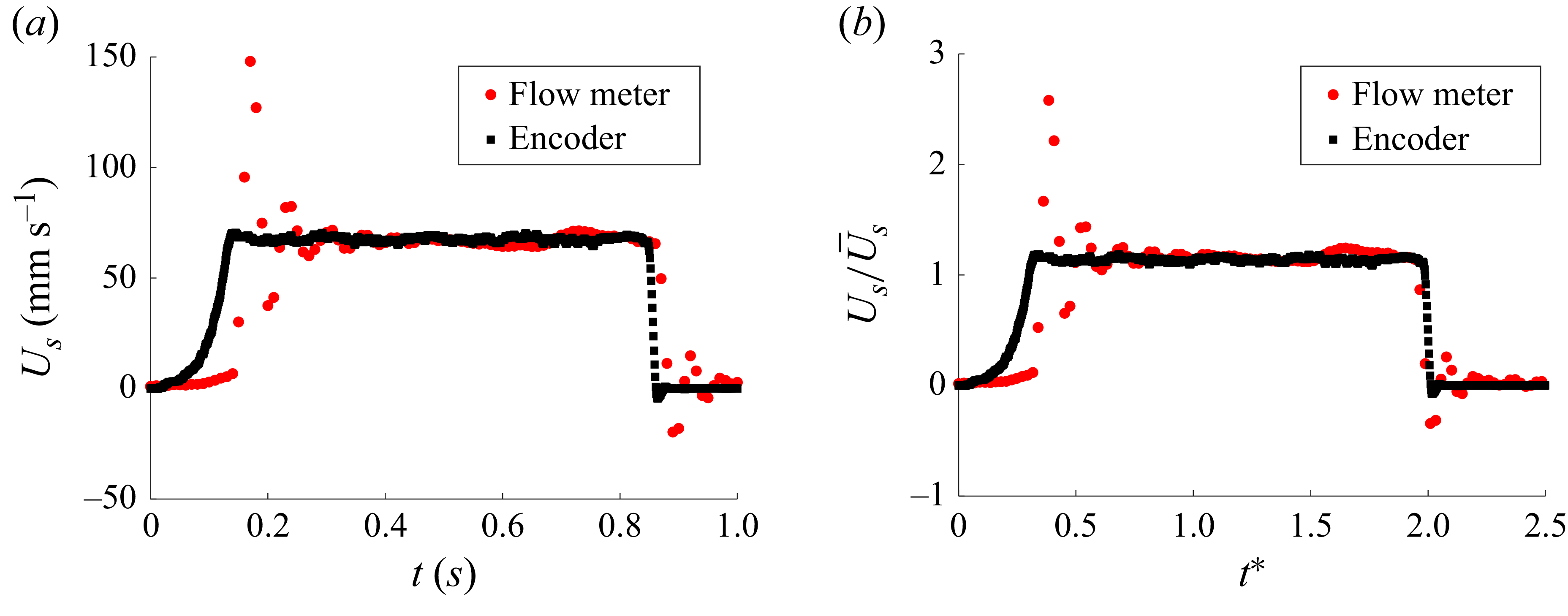
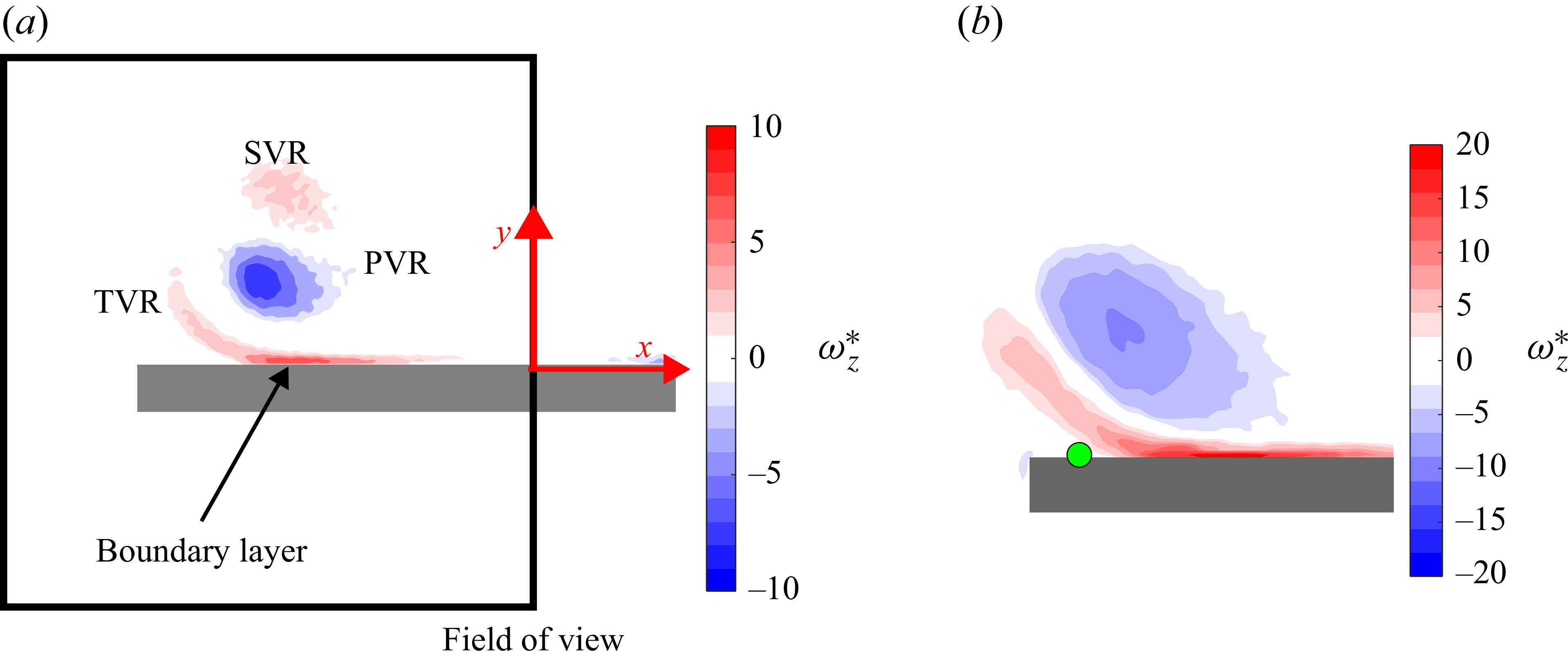
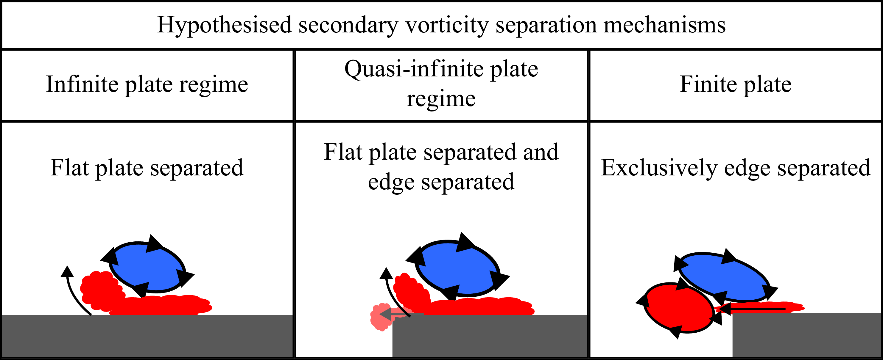


 Open access