

INTRODUCTION
Glaciers are icons of global change. Their near-global retreat during the past century is established (e.g. Leqlercq and others, Reference Leqlercq2014), leading to the widely studied hypothesis that global change must be responsible (e.g. Greuell, Reference Greuell1992; Oerlemans, Reference Oerlemans2005; Marzeion and others, Reference Marzeion, Cogley, Richter and Parkes2014). Nevertheless, Oerlemans (Reference Oerlemans2000) (and, e.g., Reichert and others, Reference Reichert, Bengtsson and Oerlemans2002; Anderson and others, Reference Anderson, Roe and Anderson2014) demonstrate that glaciers can undergo persistent kilometer-scale excursions on multi-decadal timescales, forced by natural variability inherent to a stationary climate. This leads to the need to differentiate between length fluctuations driven by natural variability and those related to a climate trend (Roe and O'Neal, Reference Roe and O'Neal2009). For any single glacier, it is fundamentally a statistical exercise to evaluate whether the observed retreat is exceptional compared with what is possible in a stationary climate. This requires accounting for all known sources of uncertainty. While several previous studies have modeled the natural fluctuations of specific glaciers (Oerlemans, Reference Oerlemans2000; Reichert and others, Reference Reichert, Bengtsson and Oerlemans2002), they have only done so far a single set of model parameters. Our study is the first to attempt a comprehensive analysis of the impact of uncertainty in glacier geometry and initial conditions, as well as climate observations.
METHOD
Three-stage model
In this study, we use the linear three-stage model of Roe and Baker (Reference Roe and Baker2014). The three-stage model was designed to emulate the response of numerical models of ice dynamics. Roe and Baker (Reference Roe and Baker2014) accurately reproduce the behavior of 1-D flowline models over a wide range of geometries applicable to alpine valley glaciers; for climate forcing of step-functions, linear trends and stochastic variability; and over timescales of decades to centuries. The three-stage model represents an improvement over earlier, similar low-order models (e.g. Oerlemans, Reference Oerlemans2001, Reference Oerlemans2005; Harrison and others, Reference Harrison, Raymond, Echelmeyer and Krimmel2003) wherein it better captures the high-frequency response of glacier dynamics. The three-stages, which can be diagnosed from ice dynamics in numerical models, are: (1) changes in interior thickness drive; (2) changes in terminus flux, which in turn drive; (3) changes in glacier length.
The three stages are represented as a linear, third-order differential equation. Anomalies in length, L′(t), from some long-term equilibrium position are given by:
 $$\left( {\displaystyle{{\rm d} \over {{\rm d}t}} + \displaystyle{1 \over {{\rm \epsilon} \tau}}} \right)^3{L}^{\prime} = \displaystyle{1 \over {{\rm \epsilon} {({\rm \epsilon} \tau )}^2}}\beta {b}^{\prime},$$
where ${\rm \epsilon} \equiv 1/\sqrt 3 $
, τ is the glacier's response time (Eqn (5)), β is a model factor that depends on the glacier geometry (Eqn (4)) and b′(t) is the anomaly in mass balance. Eqn (1) can be discretized and written as an autoregressive moving average process (Roe and Baker, Reference Roe and Baker2014). L′ depends linearly on both its own previous values as well as on b′, which reflects natural variability. The three-stage model emulates the autocorrelation function (and power spectrum) of numerical flowline models, and for appropriate parameter choices reproduces realistic length responses to climate trends and variability. See Roe and Baker (Reference Roe and Baker2014) for more details.
${\rm \epsilon} \equiv 1/\sqrt 3 $
, τ is the glacier's response time (Eqn (5)), β is a model factor that depends on the glacier geometry (Eqn (4)) and b′(t) is the anomaly in mass balance. Eqn (1) can be discretized and written as an autoregressive moving average process (Roe and Baker, Reference Roe and Baker2014). L′ depends linearly on both its own previous values as well as on b′, which reflects natural variability. The three-stage model emulates the autocorrelation function (and power spectrum) of numerical flowline models, and for appropriate parameter choices reproduces realistic length responses to climate trends and variability. See Roe and Baker (Reference Roe and Baker2014) for more details.
Low-order models like Eqn (1) are useful in several respects: the analytic solutions of such models reveal the relative importance of the physical and geometric factors that control the glacier response, and provide valuable insight into how glacier sensitivity varies under different conditions. Such models also allow for an exhaustive uncertainty analysis that would be prohibitive for more complex numerical models. It is the latter aspect that we employ in this study. We estimate the probability distributions of all the factors that control glacier sensitivity. Across that full range of uncertainty, our main result remains robust: the retreat of Hintereisferner over the last century cannot be explained by natural variability alone; and thus one must conclude that the observed retreat reflects a climate change.
Hintereisferner
Hintereisferner is an alpine glacier located in Ötztal, Austria (46.793N, 10.749E, Fig. 1). Various observations have been made during the last few decades and thus, a solid dataset is available at the World Glacier Monitoring Service (WGMS, 2012, 2013). The simple geometry of the glacier (i.e. fairly uniform slope angle, no severe overdeepening) and the favorable spatial setting (i.e. clear catchment area and valley, no glacier lake) lends confidence to the applicability of the three-stage model.
Map of Hintereisferner (Kuhn and Lambrecht, Reference Kuhn and Lambrecht2007). The blue shading indicates the glacier extent at various times since 1850.

Between 1953 and 2012, the mean elevation of the Equilibrium Line Altitude (ELA) was 3080 m.a.s.l. The ELA exceeded the highest point of the glacier (3710 m.a.s.l.) three times within the last 10 years. In 1997 the median elevation of the glacier was ~3010 m.a.s.l., and the glacier area covered ~8.5 km2 (cf. WGMS, 2012).
Trends in accumulation and summer temperature
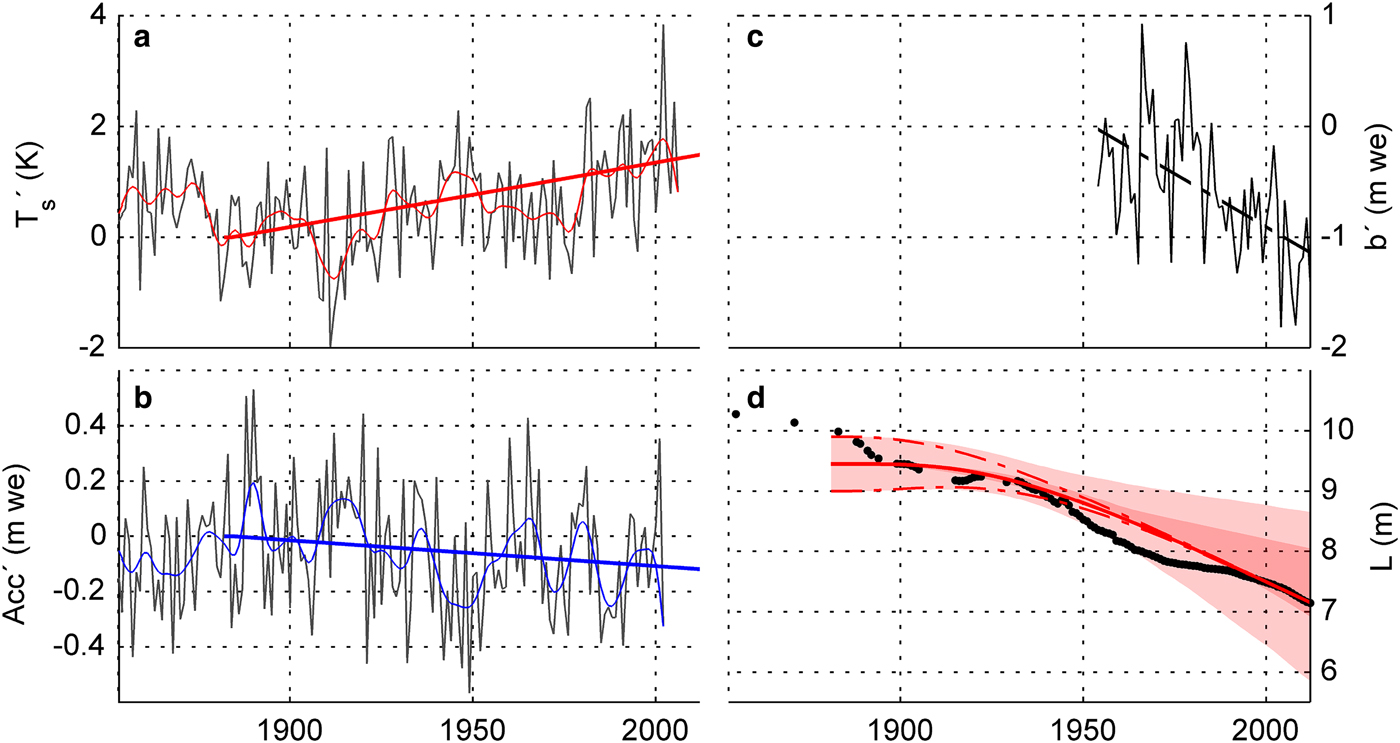
Using the HISTALP dataset (Auer and others, Reference Auer2007) for the period 1880–2010, and for the gridpoint closest to Hintereisferner, a least-squares linear regression of the average summer temperature (June–September) shows that, over the past 130 years, there has been a statistically significant warming of 1.5 K; and an insignificant change in the accumulation rate change of −0.1 m a−1 (Figs 2a, b; all accumulation values are water-equivalent in units of m a−1).
(a, b) HISTALP data for melt-season temperature and solid precipitation fluctuation at gridpoint (46.75N, 10.83E), filtered data (zero-phase distortion) and 130 year trend-lines (+1.5 K and −0.1 m w.e. per 130 years). (c) WGMS data for annual mass-balance rate at Hintereisferner (trend −1.1 m w.e. per 60 years). (d) Glacier length observations (black dots) together with model calibration using linear forcings and mid-range parameter values (solid red line); dark red shading represents uncertainty due to τ, light red shading due to α and β; dashed red lines show uncertainty in initial conditions (±2σ L).
Length observations
Length observations (black dots in Fig. 2d) record a maximum glacier length of ~10.2 km in 1855. A lichenometric study (Beschel, Reference Beschel1950) suggests that in 1770 the glacier reached 60 m further down-valley. No other study has documented a larger extent at any other time during the Holocene, which is consistent with other work (e.g. Nicolussi and Patzelt, Reference Nicolussi and Patzelt2000; Holzhauser and others, Reference Holzhauser, Magny and Zumbühl2005) showing maximal (late) Holocene glaciation ~mid-19th century. However, an anthropogenic climate forcing did not emerge until the end of the 19th century (Hartmann and others, Reference Hartmann and Stocker2013). Hence, in this study, we define the glacier extent at ~1900 as the preindustrial margin. Although there is some uncertainty in this timing, it does not affect our conclusions.
Parameter setup
In this section, we define parameters and their uncertainties. From this point on σ x is defined as the standard deviation of variable x. Roe and Baker (Reference Roe and Baker2014) allow for mass balance to be written in two ways: first,
 $$\beta {b}^{\prime} = \beta ({b}^{\prime}_{\rm w} + {b}^{\prime}_{\rm s}),$$
where ${b}^{\prime}_{\rm w}$
and
${b}^{\prime}_{\rm w}$
and ${b}^{\prime}_{\rm s}$
are anomalies in winter and summer mass balance, respectively, or second,
${b}^{\prime}_{\rm s}$
are anomalies in winter and summer mass balance, respectively, or second,
 $$\beta {b}^{\prime} = \beta {P}^{\prime} - \alpha {T}^{\prime},$$
where P′ is anomalies in solid precipitation and T′ is anomalies in melt-season temperature (June–September). The factors α and β are given by:
 $$\alpha = \displaystyle{{\mu A_{T \gt 0}} \over {wH}},\;\beta = \displaystyle{{A_{{\rm tot}}} \over {wH}},$$
where A tot is the total area, A T>0 is the area over which melting occurs; w and H are the characteristic width and thickness of the glacier in the terminus zone, and μ is the melt factor, relating ablation to melt-season temperature. The timescale τ is given by (e.g. Jóhannesson and others, Reference Jóhannesson, Raymond and Waddington1989):
 $$\tau = \displaystyle{H \over { - b_{\rm t}}},$$
where b t is the (negative) net mass balance at the terminus.
As the glacier model is linearized around its extent in 1900, geometric parameters must be estimated from the valley geometry. Table 1 shows mean and estimated standard deviations for each of these parameters based on the reconstruction of Kuhn and Lambrecht (Reference Kuhn and Lambrecht2007), reproduced in Figure 1. H was estimated using cross sections provided by Schlosser (Reference Schlosser1996) and Greuell (Reference Greuell1992). The value for b t was extrapolated from the altitudinal mass-balance profile from WGMS. To calculate (μA T>0) we use the following relation between variances of summer temperature and summer mass balance with their associated glacier areas:
 $$(\mu A_{T \gt 0})^2\sigma _{\rm T}^{\rm 2} = A_{{\rm tot}}^{\rm 2} \sigma _{b_{\rm s}}^2. $$
Model parameters (mean and standard deviation) applying to Hintereisferner at the end of the 19th century

Using this method yields a central value of (μA
T>0) = 5 ×10⁶ m3 a−1 K−1. As a secondary check, temperature and mass-balance records give a value of μ = 0.52 ma−1 K−1; this suggests A
T>0 = 9.5 km2, which is consistent with the observed WGMS vertical mass-balance gradient. Individual uncertainties are combined assuming they are independent and normally distributed, allowing variances to be summed. For example: $\sigma _\beta ^2 = \bar \beta ^2((\sigma _{\rm A}^{\rm 2} /\bar A^2) + (\sigma _{\rm w}^{\rm 2} /\bar w^2) + (\sigma _{\rm H}^{\rm 2} /\bar H^2))$
.
$\sigma _\beta ^2 = \bar \beta ^2((\sigma _{\rm A}^{\rm 2} /\bar A^2) + (\sigma _{\rm w}^{\rm 2} /\bar w^2) + (\sigma _{\rm H}^{\rm 2} /\bar H^2))$
.
Our central estimates and uncertainties (stated as standard deviations) in these geometric parameters are given in Table 1. Our parameter uncertainties are subjective, but we believe they are conservative in that they result in a broad range of uncertainty in model parameters α, β and τ. Combining uncertainties in this way we find central values {and 1σ} of
 $$\eqalign{& \alpha = 75\{ 30\} \,({\rm m}\,{\rm a}^{ - 1}\,{\rm K}^{ - 1}), \cr & \beta = 148{\kern 1pt} \{ 32\} \,({\rm unitless}), \cr & \tau = 29{\kern 1pt} \{ 10\} \,({\rm years}).} $$
There are no data available on seasonal mass-balance observations for Hintereisferner, but WGMS reports following values for the adjacent Vernagtferner (47 years of observation; 10 km distance): $\sigma _{b_{\rm s}}\!\! =\! 0.45$
,
$\sigma _{b_{\rm s}}\!\! =\! 0.45$
, $\sigma _{b_{\rm w}}\!\! = \!0.22$
(m a−1). Using the histalp dataset we apply following mask: Whenever monthly mean temperature at mid-glacier height falls below 2°C, precipitation is counted as accumulation (σ
P = 0.21 m a−1 (solid precipitation), σ
T = 0.9 K). Together with annual mass-balance observations at Hintereisferner we find annual ablation. These values agree with the ones cited above: σ
abl = 0.45 and σ
acc = 0.21 (m a−1).
$\sigma _{b_{\rm w}}\!\! = \!0.22$
(m a−1). Using the histalp dataset we apply following mask: Whenever monthly mean temperature at mid-glacier height falls below 2°C, precipitation is counted as accumulation (σ
P = 0.21 m a−1 (solid precipitation), σ
T = 0.9 K). Together with annual mass-balance observations at Hintereisferner we find annual ablation. These values agree with the ones cited above: σ
abl = 0.45 and σ
acc = 0.21 (m a−1).
Trend response
Our main goal here is to evaluate whether the model reproduces the observed trend in glacier length; we are not interested in simulating all the detailed fluctuations in the record, which are sensitive to initial conditions. Lüthi and Bauder (Reference Lüthi and Bauder2010) and Lüthi (Reference Lüthi2014) show that a low-order model similar to our three-stage model reproduces decadal fluctuations over the last century. With that in mind, we first evaluate the response of the model to the observed linear climate trends in T and P since 1880 (Figs 2a, b), using the central values of the model parameters. The model length initially changes slowly (red line in Fig. 2d), but after 110 years (1900–2010) has retreated 2.3 km, in good agreement with the observed retreat.
Having established that the central values of the model parameters simulate a reasonable value for the retreat, we next explore the range of retreats in the model, allowing for uncertainty in the initial conditions and model parameters.
Although we know the location of the glacier terminus in 1880, we do not know whether that terminus reflected an advance or retreat from its long-term equilibrium position (i.e., L′ = 0). To address this we assume that the 1880 position (L ~ 9.5 km) represents an L′ that is drawn randomly from a Gaussian probability distribution with a standard deviation of glacier length (≡ σ L ) calculated from Roe and Baker (Reference Roe and Baker2014):
 $$\sigma _{\rm L}^{\rm 2} = \displaystyle{{3\Delta t\tau} \over {16{\rm \epsilon}}} \beta ^2\sigma _{\dot {\rm b}}^{\rm 2}, $$
for Hintereisferner and mid-range parameters σ L = 225 m. In other words, this indicates the retreat since 1880 is ~13 standard deviations. This can be cast as a signal-to-noise ratio (s L = ΔL/σ L ≈ −13).
Figure 2d shows length observations at Hintereisferner (black dots) with a best estimate model emulation (mid-range parameters, solid red line) using observed climate trends as a forcing. The influence of initial conditions dissipates after a timespan of ~ 2 − 3τ (dashed red lines). The red shading represents the limits of a 1000-member Monte Carlo ensemble, where the model parameters were drawn randomly from Gaussian probability distributions. The light shading indicates uncertainty due to α and β, whereas the asymmetric dark shading refers to τ. The sensitivity to τ is smaller than to the other factors. Smaller values of τ result in a quicker response but are less sensitive to a given trend, whereas larger τ case a slower response, but are ultimately more sensitive. These two factors offset each other over the 130 year time frame. Interestingly, the central value for Hintereisferner, τ ≈ 30 years, gives nearly the maximum sensitivity of response to a 130 years trend: larger or smaller τ yield responses that are either more slowly adjusting or less sensitive (see also Roe and others (Reference Roe, Baker and Herla2017)).
LENGTH FLUCTUATION AND EXCURSION PROBABILITIES
Having calibrated the three-stage model to Hintereisferner and shown that the central parameter values can reproduce the observed retreat since 1880, we now address the question whether such a retreat might have happened due only to natural interannual variability.
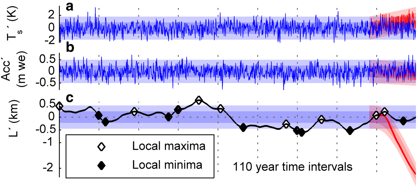
Figure 3 shows an example of a 1 ka period with a synthetic, randomly generated time series of T and P (white noise) with a variance consistent with observations, together with the resulting length fluctuations of the three-stage model using central estimates of parameters for Hintereisferner. The blue shading shows the expected ±1σ and ±2σ bounds on the climate and length variability. By construction the curves will spend ~95% of the time within the 2σ bounds, confirmed in Figure 3. Finally, the red shading shows the results if the observed climate trends are added to the last 130 years of the climate time series. Although the warming appears quite modest (Fig. 3a), the observed retreat is far larger than any fluctuation in the preceding centuries. This preliminary result emulates Oerlemans (Reference Oerlemans2000), who concluded that, for his numerical model and assumed parameters and initial conditions, the observed retreat of three glaciers (Nigardsbreen, Rhone and Franz-Josef) exceeded what was likely from natural variability. We are next able to use the computational efficiency of the three-stage model to extend the analysis to perform a comprehensive uncertainty analysis over a wide range of parameter space.
Thousand years synthetic time series of (a) melt-season temperature, (b) solid precipitation and (c) length. All panels show fluctuations around the long-term mean. The light- and dark-blue shading shows the ±1σ and ±2σ bounds, respectively. The red curves are the same, but with the observed trends (+1.5 K, −0.1 m per 130 years) added to the last 130 years of the simulation. Vertical dashed lines indicate 110 year time intervals.
Roe and Baker (Reference Roe and Baker2014) provide analytic equations for excursion probabilities (i.e., the probability of a given advance or retreat in any given interval of time). However, as they note, the formulae depend on being able to assume that successive advances and retreats are independent of each other. Although this assumption and the formulae work well over an interval of ~1000 years, we found that it was not satisfactory for intervals of time that are only a few multiples of the glacier response time (i.e., the ~100 years period of the observed retreat). Therefore we take advantage of the efficiency of the three-stage model and pursue a Monte Carlo approach: we create long (100 ka) synthetic time series of mass balance consistent with the interannual variability in a stationary climate, and use them to generate length fluctuations of the three-stage model that have parameter values drawn randomly from the uncertainty distributions that we have determined. We repeat this 1000 times and therefore get a comprehensive sampling over a broad range of the parameter space.
We present our results in Figure 4 as cumulative probability distributions for the likelihood of exceeding a given retreat in a (a) 60 years, (b) 110 years, or (c) 160 years period. Also shown as a black bar is the observed Hintereisferner retreat for the time period. In each panel the solid blue line is the central estimate.
Excursion statistics for Hintereisferner in three different intervals: dark blue shading represents uncertainty in glacier geometry and climate observations (±2σ), light blue shading represents uncertainty in initial conditions (±2σ L); solid blue lines are for central estimates of parameters; dashed lines indicate central estimate parameters and red-noise climate (giving a 75% enhancement in σ L); see text for more details.

The darker-blue shading shows the range of excursion statistics for a 2σ range of uncertainty in model parameters and the lighter-blue shading shows the additional impact of the 2σ range of uncertainty in initial conditions.
Recall that these curves show the probability of a given excursion occurring in a climate without an underlying trend. For the central estimate of the parameters (dark blue line), in all of intervals considered the chances that the observed retreat could have happened in a stationary climate are miniscule ( $p_{{\rm null}} \ll 1\% $
in all cases).
$p_{{\rm null}} \ll 1\% $
in all cases).
At the extreme end of the parameter uncertainty, it is just about possible that the retreat between 1950 and 2010 could have occurred in a stationary climate ( $p \approx 3\% $
). But for the longer intervals, not even the extreme end of the parameter uncertainty could account for the observed retreat. In other words, the null hypothesis of no climate change is falsified, and the conclusion can only be that the retreat of Hintereisferner required a definitive climate change.
$p \approx 3\% $
). But for the longer intervals, not even the extreme end of the parameter uncertainty could account for the observed retreat. In other words, the null hypothesis of no climate change is falsified, and the conclusion can only be that the retreat of Hintereisferner required a definitive climate change.
We next consider the potential role of interannual persistence in climate on the length fluctuations of Hintereisferner. Previous studies (Reichert and others, Reference Reichert, Bengtsson and Oerlemans2002; Roe and Baker, Reference Roe and Baker2016) have shown that adding even a small amount of persistence can enhance glacier fluctuations: a small chance that 1 year's climate has the same sign anomaly as the following year enhances the cumulative climate forcing experienced by the glacier.
The degree of persistence in the climate around Hintereis-ferner is unclear. For the interval between 1880 and 2012, evaluating the best-fit autoregression process to the histalp temperature data using standard methods (e.g. Box and others, Reference Box, Jenkins and Reinsel2008) suggests the temperature data is best characterized by white noise (i.e., no persistence). An alternative measure of persistence is the slope of the power spectrum (e.g. Beran, Reference Beran1994), for which we obtain − 0.25 ± 0.33 (2σ bounds). This suggests that some persistence may be present, but that it is not formally statistically significant at the 5% level. The precipitation record indicates less persistence, and which is also not significant at the 5% level. This is consistent with the overall conclusions of Burke and Roe (Reference Burke and Roe2014) and Medwedeff and Roe (Reference Medwedeff and Roe2017), that interannual persistence in mass balance is generally small, with a statistical significance that is at best marginal.
Nevertheless, it is reasonable to suppose that some level of interannual persistence exists, and following Roe and Baker (Reference Roe and Baker2016) we pursue a what-if approach: if such persistence indeed exists, what is its impact on glacier excursions? Roe and Baker (Reference Roe and Baker2016) provide a derivation of the impact of power-law persistence on glacier variability for the three-stage model. For τ = 30 years and a power-law slope of −0.25, their formula indicates that σ L increases by a factor of ~1.75. The dashed lines in Figure 4 show the impact on the excursion probabilities of such persistence, for the central set of model parameters.
Such interannual persistence increases the magnitude of retreats that occur even without a climate change, but even for the shortest interval the probability of the observed retreat happening in a stationary climate remains negligible (p < 1%).
ATTRIBUTION OF THE REGIONAL CLIMATE CHANGE
In our analyses we have shown that the regional climate must have changed during the last century for Hintereisferner to experience such a drastic retreat. So far, our approach does not answer the question what this change is due to. Consequently, in the following section we ask whether the temperature change at Hintereisferner is consistent with model predictions attributing the change to natural and anthropogenic causes.
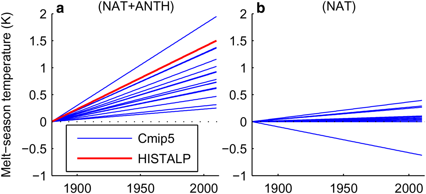
We have extracted data from 15 different global circulation models of the Coupled Model Intercomparison Project 5 (CMIP5). This includes temperature time series for the Hintereisferner model gridpoint; one set simulates temperature history with only natural forcing (NAT), the other set also includes anthropogenic forcing (NAT & ANTH).
Figure 5 shows the trendlines for these different melt-season temperature time series for the period 1880–2010. The models somewhat underestimate the observed warming on average, although natural variability may account for some part of the difference. Panel (a) also shows the observed histalp trend, which is at the higher end, but within the range of CMIP5 model simulation trends. The key point is that in the naturally forced model runs none of the trends are as large as the observed one. Therefore, natural variability, as represented by the CMIP5 models, cannot account for the observed temperature trend. However, when anthropogenic forcing is included, the CMIP5 model ensemble is consistent with the observed trend.
Best-fit trend lines to CMIP5 model simulations for melt-season temperature at Hintereisferner (blue lines); (a) with natural and anthropogenic forcings (HISTALP trendline is included in red), (b) with only natural forcings.
DISCUSSION
An analytical glacier model has been used to ask the question: does the observed retreat of Hintereisferner exceed what can occur due to the natural interannual variability, that occurs even in a stationary climate? Our answer is an emphatic yes for the period of 1850–2012, although variability could conceivably account for retreat during shorter intervals. Two independent approaches were used to calculate the model coefficients: first observations of mass-balance statistics and glacier geometry and second, a calibration to observed length change. The agreement between the two approaches indicates internal consistency. The efficiency of the three-stage model allows us to consider an uncertainty range that takes into account uncertainty in glacier geometry, parameters and initial conditions. One caveat in this uncertainty analysis is that we assume the various geometric properties are independent. For instance, we include cases like an increased slope angle together with an increased ice thickness, whereas in reality these properties are correlated and an increased slope angle would lead to a decreasing ice thickness. This anticorrelation would tend to reduce the uncertainty range.
A comparison of the observed trend with that represented in anthropologically forced and unforced ensembles of global circulation models suggests that the observed trend cannot be explained by natural variability or natural forcing.
Pursuing an independent approach that used the signal-to-noise ratio of observed climate trends, Roe and others (Reference Roe, Baker and Herla2017) conclude that, for the period 1880–2010 (ΔL = −2800 m), the median signal-to-noise ratio for Hintereisferner (and 2σ bounds) is s L = −13(−10, −16). Our parameter-uncertainty-based calculations give σ L = 225(160, 290) m, which for this same interval of time translates to s L = −13(−10, −18). It is encouraging that these two independent approaches give such similar estimates and ranges. It strengthens the main conclusion of this study: Hintereisferner has retreated far beyond what can be explained by natural variability and is therefore definitive evidence of the climate change that has occurred over the last 150 years.
ACKNOWLEDGEMENTS
We are grateful to Marcia Baker for valuable ideas and suggestions. F. H. thanks the Ice and Climate research unit of the Institute of Atmospheric and Cryospheric Sciences, as well as the University of Innsbruck for their financial support of travel expenses. B. M. was supported by the Austrian Science Fund (FWF): P25362. We acknowledge the World Climate Research Programme's Working Group on Coupled Modeling, which is responsible for CMIP, and we thank the climate modeling groups for producing and making available their model output. For CMIP the US Department of Energy's Program for Climate Model Diagnosis and Intercomparison provides coordinating support and led development of software infrastructure in partnership with the Global Organization for Earth System Science Portals.


 Open access