


1. Introduction
The load-sharing system has a wide application in reliability practice, and in such a context, system components usually share the workload while they are in operation. Take for example, fibers in composite (Rosen [Reference Rosen19]), two kidneys of a patient (Gross et al. [Reference Gross, Clark and Liu8]), pumps in a hydraulic system (Taghipour [Reference Taghipour25]), cables in a suspension bridge and parallel generator systems (Elmakias [Reference Elmakias6]).
The modeling of load-sharing systems has been extensively studied in the past decades. Among the first to study multi-component load-sharing systems, Ross [Reference Ross20] modeled the instantaneous failure rate of one component as a function of the set of other working components. For the load-sharing parallel system with the component failure rate being linear with respect to the load at any time, Schechner [Reference Schechner21] examined the aging property of the system and the ordering results of different systems. Afterward, Scheuer [Reference Scheuer22] derived the reliability function of load-sharing  $k$-out-of- $n$ systems in the context that component lifetimes are of independent and identical exponential distribution and the component failure rate is determined by the number of failed components. Under the assumption of repairable components and imperfect switching, Shao and Lamberson [Reference Shao and Lamberson24] analyzed the reliability and availability of the load-sharing $k$-out-of- $n$ system based on a Markov model. Subsequently, Liu [Reference Liu16] built the reliability of load-sharing $k$-out-of- $n$ systems in the setting that component lifetime distribution follows the decelerated failure time model, and Tang and Zhang [Reference Tang and Zhang27] proposed a new model for load-sharing $k$-out-of- $n$ system based on the capacity flow approach. Later on, Yun and Cha [Reference Yun and Cha28] generalized the model of two-component load-sharing parallel systems in Liu [Reference Liu16] by introducing the virtual age to component lifetime after the transformation of load.
In recent decades, several researchers have made efforts to further investigate other aspects of load-sharing systems, including parameter inference, periodic inspection optimization, preventive maintenance, stochastic comparisons of system lifetimes, and so on. Remarkably, Balakrishnan et al. [Reference Balakrishnan, Beutner and Kamps1] discussed the parameter estimation of load-sharing system by means of link function in the sequential order statistics model. Taghipour and Kassaei [Reference Taghipour and Kassaei26] developed a model to find the optimal inspection interval for a load-sharing  $k$-out-of- $n$ system in the sense of minimizing the total expected cost incurred over one system life cycle. Finkelstein and Hazra [Reference Finkelstein and Hazra7] studied the optimal allocation strategy for one load-sharing redundant component of series and parallel systems, and it was shown that under certain assumptions allocating the redundant component to the stochastic weakest (strongest) component of a series (parallel) system is the best strategy to achieve the maximal system reliability. Afterward, for load-sharing systems with identically distributed component lifetimes and subject to continuous degradation, Liu et al. [Reference Liu, Xie and Kuo15] investigated system maintenance and design decisions, and Zhao et al. [Reference Zhao, Liu and Liu29] further examined the parameter estimation related to this model. In addition, Mies and Bedbur [Reference Mies and Bedbur18] derived exact finite-sample inference procedures to test the load-sharing parameters and the specific nonparametric baseline distribution of component lifetimes in the setting of load-sharing systems. Recently, Li et al. [Reference Li, Fang and Li11] developed the stochastic comparison between the two-component load-sharing parallel system and the baseline component lifetimes.
For load-sharing systems, component lifetimes are usually assumed to be mutually independent when the system is put into operation. At the beginning, the workload is shared by all components. However, it has to be shared by the remaining active components once one component fails. As a consequence, those active components get a higher component failure rate due to an increase of workload once a component failure occurs. As common sense, system components interact with each other and then their marginal lifetimes finally acquire stochastic dependence. Intuitively, component marginal lifetimes of a load-sharing system are positively stochastic dependent. Naturally, it is of both theoretical and practical interest to quantify the stochastic dependence of marginal lifetimes in the setting of load-sharing systems. In the main stream of the literature in this line, most of the research focus on the study of system reliability, and as far as we know, few of references pay attention to the stochastic dependence structure of marginal lifetimes except for Bassan and Spizzichino [Reference Bassan and Spizzichino3], which is among the first to examine the total positive property of two marginal lifetimes in the model of Ross [Reference Ross20] for the load-sharing parallel system with two component lifetimes having a common exponential distribution. In fact, the model of Bassan and Spizzichino [Reference Bassan and Spizzichino3] can be viewed as the load-sharing model of Yun and Cha [Reference Yun and Cha28] with component lifetimes having a common exponential distribution and subject to the same decelerating factor. In this study, we further investigate the stochastic dependence between the marginal lifetimes of the load-sharing parallel system of two components under the framework of load-sharing model of Yun and Cha [Reference Yun and Cha28]. We generalize the result of Bassan and Spizzichino [Reference Bassan and Spizzichino3] to the circumstance that component lifetimes have possibly different exponential distributions. Also, we develop sufficient conditions for the positive quadrant dependent property of marginal lifetimes of two components with general continuous probability distributions, and this complements the result of Bassan and Spizzichino [Reference Bassan and Spizzichino3].
The remainder of the manuscript is organized as follows. In Section 2, we review some related concepts, including monotone aging properties and notions of stochastic dependence, and introduce the preliminary of the load-sharing reliability model. In Section 3, we derive the joint survival function of the two component lifetimes in the setting of load-sharing parallel structure and further show that the marginal lifetimes are positive quadrant dependent. In Section 4, we pay special attention to system components both having exponential lifetime distributions and prove that the marginal lifetimes are totally positive of order 2 in the setting of load-sharing parallel systems. In Section 5, we present two simple applications of the new results. In Section 6, we summarize the study. All proofs of the main theorems are deferred to the appendix.
For convenience, in the coming sections, we denote  $\mathcal{B}(p)$ the Bernoulli distribution with probability of success $p\in(0,1)$, $\mathcal{E}(\lambda)$ the exponential distribution with hazard rate $\lambda \gt 0$, and $\mathcal{W}(\lambda,\alpha)$ the Weibull distribution with survival function $e^{-(\lambda x)^\alpha}$ for $\lambda,\alpha,x \gt 0$. Also, “ $\stackrel{\textrm{st}}{=}$” and “ $\stackrel{\textrm{sgn}}{=}$” stand for the stochastic equivalence (i.e., both sides have the same cumulative distribution function) and the equivalence in sign (i.e., both sides have the same sign), respectively. Throughout the manuscript, the cdf and pdf are abbreviations of “cumulative distribution function” and “probability density function,” respectively, and increasing and decreasing stand for “nondecreasing” and “nonincreasing,” respectively.
2. Preliminaries
Before proceeding to the main results on the stochastic dependence of the two marginal lifetimes in the setting of the load-sharing parallel system, let us recall some important notions, which are related to the main results to be developed in Sections 3 and 4.
2.1. Some related notions
In system engineering practice, components usually experience aging due to degradation and wear-out, and also component lifetimes are interdependent due to the interaction and common environment. Thus, it is of practical interest to take aging behavior and stochastic dependence into account in modeling engineering reliability and system safety.
A random vector  $(S,T)$ is said to be positive quadrant dependent, denoted as PQD $(S,T)$, if
 \begin{equation*}
\mathrm{P}(S \gt s,T \gt t)\ge \mathrm{P}(S \gt s)\mathrm{P}(T \gt t),
\qquad\mbox{for any}\ s\ \mbox{and}\ t.
\end{equation*}
\begin{equation*}
\mathrm{P}(S \gt s,T \gt t)\ge \mathrm{P}(S \gt s)\mathrm{P}(T \gt t),
\qquad\mbox{for any}\ s\ \mbox{and}\ t.
\end{equation*}  $T$ is said to be stochastically increasing in $S$ (denoted as SI( $T|S$)) if
 \begin{equation*}
\mathrm{P}(T \gt t\mid S=s)\qquad\mbox{is increasing in}\ s\ \mbox{for any}\ t.
\end{equation*}
\begin{equation*}
\mathrm{P}(T \gt t\mid S=s)\qquad\mbox{is increasing in}\ s\ \mbox{for any}\ t.
\end{equation*} A random vector  $(S,T)$ with joint pdf $\ell(s,t)$ is said to be totally positive of order 2 (TP2) if
 \begin{equation*}
\ell(s_1,t_1)\ell(s_2,t_2)\ge \ell(s_1,t_2)\ell(s_2,t_1),\qquad
\mbox{for}\ s_1 \lt s_2\ \mbox{and}\ t_1 \lt t_2.
\end{equation*}
\begin{equation*}
\ell(s_1,t_1)\ell(s_2,t_2)\ge \ell(s_1,t_2)\ell(s_2,t_1),\qquad
\mbox{for}\ s_1 \lt s_2\ \mbox{and}\ t_1 \lt t_2.
\end{equation*}Note that the following chain of implications is well-known.
 \begin{equation}
\mathrm{TP}2(S,T)\Longrightarrow \mathrm{SI}(T\,|\,S) \Longrightarrow \mathrm{PQD}(S,T).
\end{equation}
\begin{equation}
\mathrm{TP}2(S,T)\Longrightarrow \mathrm{SI}(T\,|\,S) \Longrightarrow \mathrm{PQD}(S,T).
\end{equation} A random variable (r.v.)  $S$ is said to be of increasing failure rate (IFR) if
 \begin{equation*}
\mathrm{P}(S \gt s+t)/\mathrm{P}(s)\qquad\mbox{is decreasing in}\ s\ \mbox{for any}\ t.
\end{equation*}
\begin{equation*}
\mathrm{P}(S \gt s+t)/\mathrm{P}(s)\qquad\mbox{is decreasing in}\ s\ \mbox{for any}\ t.
\end{equation*}For a load-sharing parallel system, we will discuss the PQD property of the ultimate marginal lifetimes in the setting that two component lifetimes are both IFR. We refer readers to Barlow and Proschan [Reference Barlow and Proschan2], Lai and Xie [Reference Lai and Xie10], Shaked and Shanthikumar [Reference Shaked and Shanthikumar23], and Li and Li [Reference Li and Li13] for a comprehensive discussion on aging notions and positive dependence.
2.2. Load-sharing parallel systems
Consider a parallel system of two components  $\mathcal{C}_1$ and $\mathcal{C}_2$. Suppose in the context of full load $\mathcal{C}_1$ and $\mathcal{C}_2$ have lifetimes $X_1, X_2$ with cdf’s $F_1, F_2$, respectively. Denote $\bar{F}_1=1-F_1$ and $\bar{F}_2=1-F_2$ their survival functions and $f_1$ and $f_2$ their pdf’s, respectively. Assume that when the system starts its operation, the total load is shared by $\mathcal{C}_1$ and $\mathcal{C}_2$ with assignment proportions $\alpha\in(0,1)$ and $\bar\alpha=1-\alpha$, respectively. Once the first component failure occurs, the other component takes the full load and continues its operation. In the mode of load-sharing, denote for $\mathcal{C}_1$ and $\mathcal{C}_2$ lifetimes $\tilde{X}_1, \tilde{X}_2$ with cdf’s $\tilde{F}_1,\tilde{F}_2$, respectively. Motivated by the idea of the decelerating lifetime, Yun and Cha [Reference Yun and Cha28] introduced the model of
 \begin{equation*}\tilde{F}_1(t)=F_1(g^{}_1(\alpha)t)\quad\mbox{and}\quad \tilde{F}_2(t)=F_2(g^{}_2(\bar\alpha)t),\qquad\mbox{for any}\ t\ge0,\end{equation*}
 where  $g^{}_i(0)=0$ and the decelerating factor $g^{}_i(\alpha)\in[0,1]$ is strictly increasing in $\alpha$, $i=1,2$.
Recall that  $S$ with cdf $F$ is said to be smaller than $T$ with cdf $G$ in the usual stochastic order (denoted as $S\le_{\textrm{st}}T$) if $\bar{F}(x)\le\bar{G}(x)$ for all $x$. It is clear that $X_1\le_{\textrm{st}}\tilde{X}_1$ and $X_2\le_{\textrm{st}}\tilde{X}_2$, i.e., a stochastic smaller lifetimes under the full load.
On the other hand, for the two components having been in operation in the mode of load sharing during  $(0,u]$ and without a failure, denote $\mathcal{C}_{1,u}$ and $\mathcal{C}_{2,u}$ their respective versions which just proceed to operating from time $u$ on in the mode of full load. Similar to the virtual age model, $\mathcal{C}_{i,u}$ is assumed to attain the virtual age $w_i(u)$ under the full load immediately after the change of regime at time $u$, where $w_i(0)=0$ and $w_i(u)\in(0,u]$ is increasing in $u\ge0$, $i=1,2$. As thus, $\mathcal{C}_{i,u}$ attains survival function
 \begin{equation*}
\mathrm{P}(X_i \gt w_i(u)+t\,|\,X_i \gt w_i(u))=\bar{F}_i(w_i(u)+t)/\bar{F}_i(w_i(u)),
\qquad\mbox{for all}\ u,t\ge0, i=1,2.
\end{equation*}
\begin{equation*}
\mathrm{P}(X_i \gt w_i(u)+t\,|\,X_i \gt w_i(u))=\bar{F}_i(w_i(u)+t)/\bar{F}_i(w_i(u)),
\qquad\mbox{for all}\ u,t\ge0, i=1,2.
\end{equation*} Let  $X_1^*$ and $X_2^*$ be excess lifetimes of $\mathcal{C}_1$ and $\mathcal{C}_2$ right after the change of regime at the failure time of $\mathcal{C}_2$ and $\mathcal{C}_1$, respectively, and denote the indicator $\delta=I(\tilde{X}_2 \gt \tilde{X}_1)$. Then, for $t,u\ge0$,
 \begin{equation}
\left\{\begin{array}{l}
\mathrm{P}(X_1^*=0\,|\, \tilde{X}_2=u, \delta=1)=1,\\
\mathrm{P}(X_1^* \gt t\,|\, \tilde{X}_2=u, \delta=0)=\bar{F}_1(w_1(u)+t)/\bar{F}_1(w_1(u)),
\end{array}\right.
\end{equation}
\begin{equation}
\left\{\begin{array}{l}
\mathrm{P}(X_1^*=0\,|\, \tilde{X}_2=u, \delta=1)=1,\\
\mathrm{P}(X_1^* \gt t\,|\, \tilde{X}_2=u, \delta=0)=\bar{F}_1(w_1(u)+t)/\bar{F}_1(w_1(u)),
\end{array}\right.
\end{equation} \begin{equation}
\left\{\begin{array}{l}
\mathrm{P}(X_2^*=0\,|\, \tilde{X}_1=u,\delta=0)=1,\\
\mathrm{P}(X_2^* \gt t\,|\, \tilde{X}_1=u, \delta=1)=\bar{F}_2(w_2(u)+t)/\bar{F}_2(w_2(u)).
\end{array}\right.
\end{equation}
\begin{equation}
\left\{\begin{array}{l}
\mathrm{P}(X_2^*=0\,|\, \tilde{X}_1=u,\delta=0)=1,\\
\mathrm{P}(X_2^* \gt t\,|\, \tilde{X}_1=u, \delta=1)=\bar{F}_2(w_2(u)+t)/\bar{F}_2(w_2(u)).
\end{array}\right.
\end{equation} Also it holds that, for  $u\ge0$,
 \begin{equation}
\mathrm{P}(\delta=0\,|\, \tilde{X}_2=u)=\bar{F}_1(g^{}_1(\alpha)u)=1-\mathrm{P}(\delta=1\,|\, \tilde{X}_2=u),
\end{equation}
\begin{equation}
\mathrm{P}(\delta=0\,|\, \tilde{X}_2=u)=\bar{F}_1(g^{}_1(\alpha)u)=1-\mathrm{P}(\delta=1\,|\, \tilde{X}_2=u),
\end{equation} \begin{equation}
\mathrm{P}(\delta=1\,|\, \tilde{X}_1=u)=\bar{F}_2(g^{}_2(\bar\alpha)u)=1- \mathrm{P}(\delta=0\,|\, \tilde{X}_1=u).
\end{equation}
\begin{equation}
\mathrm{P}(\delta=1\,|\, \tilde{X}_1=u)=\bar{F}_2(g^{}_2(\bar\alpha)u)=1- \mathrm{P}(\delta=0\,|\, \tilde{X}_1=u).
\end{equation} Let  $T_1$ and $T_2$ be ultimate survival times of components $\mathcal{C}_1$ and $\mathcal{C}_2$ in the setting of load-sharing parallel system, respectively. Then, it follows immediately that
 \begin{equation*}
(T_1,T_2)\stackrel{\textrm{st}}{=}
\big(\delta\tilde{X}_1+(1-\delta)(\tilde{X}_2+X_1^*),
(1-\delta)\tilde{X}_2+\delta(\tilde{X}_1+X_2^*)\big),
\end{equation*}
\begin{equation*}
(T_1,T_2)\stackrel{\textrm{st}}{=}
\big(\delta\tilde{X}_1+(1-\delta)(\tilde{X}_2+X_1^*),
(1-\delta)\tilde{X}_2+\delta(\tilde{X}_1+X_2^*)\big),
\end{equation*}and thus, the system lifetime
 \begin{equation*}T=\max\{T_1,T_2\}=\delta(\tilde{X}_1+X_2^*)+(1-\delta)(\tilde{X}_2+X_1^*).\end{equation*}
 This is exactly the model of Yun and Cha [Reference Yun and Cha28], which focuses on developing the system reliability function. In this note, we devote to studying the stochastic dependence of the ultimate component lifetimes  $T_1$ and $T_2$ of such a load-sharing parallel system. Particularly, the decelerating factors $g_1(\alpha)$ and $g_2(\bar\alpha)$ are treated as constants, i.e., $c_1=g_1(\alpha)$ and $c_2=g_2(\bar\alpha)$ in the rest of this manuscript.
3. Positive quadrant dependence of marginal lifetimes
Now, we are ready to present the joint probability distribution of the two ultimate marginal lifetimes  $(T_1,T_2)$.
Theorem 3.1. The survival function of  $(T_1,T_2)$ is
 \begin{eqnarray*}
&&\mathrm{P}(T_1 \gt x,T_2 \gt y)\\
&=&\left\{\begin{array}{ll}
\bar{F}_1(c_1y) \bar{F}_2(c_2y)
+\displaystyle\int_x^y \frac{\bar{F}_2(w_2(u)+y-u)} {\bar{F}_2(w_2(u))}\bar{F}_2(c_2u)\,\mathrm{d} F_1(c_1u), &\mbox{if}\ y \gt x\ge 0,\\[1em]
\bar{F}_1(c_1x) \bar{F}_2(c_2x)
+\displaystyle\int_y^x \frac{\bar{F}_1(w_1(u)+x-u)} {\bar{F}_1(w_1(u))}\bar{F}_1(c_1u)\,\mathrm{d} F_2(c_2u),&\mbox{if}\ x\ge y\ge 0.
\end{array}\right.
\end{eqnarray*}
\begin{eqnarray*}
&&\mathrm{P}(T_1 \gt x,T_2 \gt y)\\
&=&\left\{\begin{array}{ll}
\bar{F}_1(c_1y) \bar{F}_2(c_2y)
+\displaystyle\int_x^y \frac{\bar{F}_2(w_2(u)+y-u)} {\bar{F}_2(w_2(u))}\bar{F}_2(c_2u)\,\mathrm{d} F_1(c_1u), &\mbox{if}\ y \gt x\ge 0,\\[1em]
\bar{F}_1(c_1x) \bar{F}_2(c_2x)
+\displaystyle\int_y^x \frac{\bar{F}_1(w_1(u)+x-u)} {\bar{F}_1(w_1(u))}\bar{F}_1(c_1u)\,\mathrm{d} F_2(c_2u),&\mbox{if}\ x\ge y\ge 0.
\end{array}\right.
\end{eqnarray*} As a direct consequence of Theorem 3.1, the pdf of  $(T_1,T_2)$ is derived as
 \begin{equation}
f(x,y)=\frac{\partial^2} {\partial x\partial y}\mathrm{P}(T_1 \gt x,T_2 \gt y) =c_1\frac{f_2(w_2(x)+y-x)} {\bar{F}_2(w_2(x))}\bar{F}_2(c_2x) f_1(c_1x),\quad\mbox{for}\ y \gt x\ge 0,
\end{equation}
\begin{equation}
f(x,y)=\frac{\partial^2} {\partial x\partial y}\mathrm{P}(T_1 \gt x,T_2 \gt y) =c_1\frac{f_2(w_2(x)+y-x)} {\bar{F}_2(w_2(x))}\bar{F}_2(c_2x) f_1(c_1x),\quad\mbox{for}\ y \gt x\ge 0,
\end{equation} \begin{equation}
f(x,y)=\frac{\partial^2} {\partial x\partial y}\mathrm{P}(T_1 \gt x,T_2 \gt y)=c_2\frac{f_1(w_1(y)+x-y)} {\bar{F}_1(w_1(y))}\bar{F}_1(c_1y) f_2(c_2y),\quad\mbox{for}\ x\ge y\ge 0.
\end{equation}
\begin{equation}
f(x,y)=\frac{\partial^2} {\partial x\partial y}\mathrm{P}(T_1 \gt x,T_2 \gt y)=c_2\frac{f_1(w_1(y)+x-y)} {\bar{F}_1(w_1(y))}\bar{F}_1(c_1y) f_2(c_2y),\quad\mbox{for}\ x\ge y\ge 0.
\end{equation} Also, by setting  $y=0$ and $x=0$ in $\mathrm{P}(T_1 \gt x,T_2 \gt y)$ for $x\ge y\ge0$ and $y \gt x\ge0$, respectively, the marginal survival functions of $T_1$ and $T_2$ are obtained as
 \begin{equation}
\mathrm{P}(T_1 \gt x)
=\bar{F}_1(c_1x) \bar{F}_2(c_2x)
+\int_0^x \frac{\bar{F}_1(w_1(u)+x-u)} {\bar{F}_1(w_1(u))}\bar{F}_1(c_1u)\,\mathrm{d} F_2(c_2u),
\; x\ge 0,
\end{equation}
\begin{equation}
\mathrm{P}(T_1 \gt x)
=\bar{F}_1(c_1x) \bar{F}_2(c_2x)
+\int_0^x \frac{\bar{F}_1(w_1(u)+x-u)} {\bar{F}_1(w_1(u))}\bar{F}_1(c_1u)\,\mathrm{d} F_2(c_2u),
\; x\ge 0,
\end{equation} \begin{equation}
\mathrm{P}(T_2 \gt y)
=\bar{F}_1(c_1y) \bar{F}_2(c_2y)
+\int_0^y \frac{\bar{F}_2(w_2(u)+y-u)} {\bar{F}_2(w_2(u))}\bar{F}_2(c_2u)\,\mathrm{d} F_1(c_1u),
\; y\ge 0.
\end{equation}
\begin{equation}
\mathrm{P}(T_2 \gt y)
=\bar{F}_1(c_1y) \bar{F}_2(c_2y)
+\int_0^y \frac{\bar{F}_2(w_2(u)+y-u)} {\bar{F}_2(w_2(u))}\bar{F}_2(c_2u)\,\mathrm{d} F_1(c_1u),
\; y\ge 0.
\end{equation} Intuitively, if one component fails at an early age, then the other has to operate under the full load and thus will fail more quickly. In contrast, if one of them operates for a longer time, then the other is exposed to the full load later and thus will last for a longer time also. Naturally, one conjectures that the ultimate marginal lifetimes  $(T_1,T_2)$ are actually PQD. To the best of our knowledge, no such conclusion was reported yet in the literature. As the first main result, Theorem 3.2 presents one sufficient condition for $(T_1,T_2)$ to be PQD.
Theorem 3.2. Suppose component lifetimes  $X_1$ and $X_2$ are both IFR. If $w_1(u)\ge c_1u$, $w_2(u)\ge c_2u$ and $c_1\le w'_1(u)\le 1$, $c_2\le w'_2(u)\le 1$ for any $u\ge0$, then, $(T_1,T_2)$ is PQD.
Recall that Bassan and Spizzichino [Reference Bassan and Spizzichino3] proved that the ultimate marginal lifetimes  $(T_1,T_2)$ is TP $_2$ when two component lifetimes have a common exponential distribution and share a common decelerating factor. Theorem 3.2 asserts that two ultimate marginal lifetimes of the load-sharing parallel system are PQD if both component lifetimes are of IFR and the virtual age dominates the decelerating factor, and thus it serves as one complement of Bassan and Spizzichino [Reference Bassan and Spizzichino3].
In view of the chain of implications of (2.1), naturally, one wonders whether PQD property of the two ultimate marginal lifetimes can be upgraded to some stronger notion of stochastic dependence. Note that  $\mathcal{W}(3,2)$ and $\mathcal{W}(1,2)$ are both IFR. Based on Example 4.3 of Section 4, we come up with a negative answer in the general context of Theorem 3.2. Also, in Example 3.3 below, we show that the PQD property of $(T_1,T_2)$ in Theorem 3.2 will be jeopardized if either conditions on virtual ages and decelerating factors or the IFR properties of $X_1$ and $X_2$ are violated.
Example 3.3. (i) Let  $X_1\sim\mathcal{W}(1,2)$ and $X_2\sim\mathcal{W}(1,3)$, both of which are IFR. Also, for $\omega_1(u)=\omega_2(u)=0.01u$ for $u\ge0$ and $c_1=c_2=0.99$, it is easy to verify that the conditions on the virtual ages and decelerating factors in Theorem 3.2 are violated.
For  $y \gt x\ge0$, three survival functions associated with $(T_1,T_2)$ are
 \begin{eqnarray*}
\mathrm{P}(T_1 \gt x)&=&e^{-[(0.99x)^2+(0.99x)^3]}+3\cdot0.99^3\int_0^x u^2e^{-(x-0.99u)^2+(0.01u)^2-(0.99u)^3-(0.99u)^2}\,\mathrm{d} u,\\
\mathrm{P}(T_2 \gt y)&=&e^{-[(0.99y)^2+(0.99y)^3]}+2\cdot0.99^2\int_0^y ue^{-(y-0.99u)^3+(0.01u)^3-(0.99u)^3-(0.99u)^2}\,\mathrm{d} u,\\
\mathrm{P}(T_1 \gt x,T_2 \gt y)&=&e^{-[(0.99y)^2+(0.99y)^3]}+2\cdot0.99^2\int_x^y ue^{-(y-0.99u)^3+(0.01u)^3-(0.99u)^3-(0.99u)^2}\,\mathrm{d} u.
\end{eqnarray*}
\begin{eqnarray*}
\mathrm{P}(T_1 \gt x)&=&e^{-[(0.99x)^2+(0.99x)^3]}+3\cdot0.99^3\int_0^x u^2e^{-(x-0.99u)^2+(0.01u)^2-(0.99u)^3-(0.99u)^2}\,\mathrm{d} u,\\
\mathrm{P}(T_2 \gt y)&=&e^{-[(0.99y)^2+(0.99y)^3]}+2\cdot0.99^2\int_0^y ue^{-(y-0.99u)^3+(0.01u)^3-(0.99u)^3-(0.99u)^2}\,\mathrm{d} u,\\
\mathrm{P}(T_1 \gt x,T_2 \gt y)&=&e^{-[(0.99y)^2+(0.99y)^3]}+2\cdot0.99^2\int_x^y ue^{-(y-0.99u)^3+(0.01u)^3-(0.99u)^3-(0.99u)^2}\,\mathrm{d} u.
\end{eqnarray*} It is seen in Figure 1(a) that  $\mathrm{P}(T_1 \gt x,T_2 \gt y)\ge\mathrm{P}(T_1 \gt x)\mathrm{P}(T_2 \gt y)$ is not always true for $x\in[0.3,0.4]$ and $y\in[0.8,2]$. Hence, $(T_1,T_2)$ is not PQD.
The surface  $\mathrm{P}(T_1 \gt x,T_2 \gt y)-\mathrm{P}(T_1 \gt x)\mathrm{P}(T_2 \gt y)$ (a) $x\in[0.3,0.4]$ and $y\in[0.8,2]$ (b) $1.3\le y\le x\le 2$.

Figure 1 Long description
The image A shows a three-dimensional surface plot representing the dependence measure P(T subscript 1 greater than x, T subscript 2 greater than y) minus P(T subscript 1 greater than x) P(T subscript 2 greater than y). The x-axis is labeled x, ranging from 0.3 to 0.4 and the y-axis is labeled y, ranging from 0.8 to 2. The surface decreases as x increases and y decreases, with values near zero at lower x and higher y. The image B shows a similar plot with x ranging from 1.3 to 2 and y ranging from 1.3 to 2. The surface increases with x and y, showing positive values across the domain. Both plots are unitless, illustrating the behavior of the dependence measure across different ranges. Notable regions include near-zero values in image A and positive values in image B, indicating different dependence behaviors in each panel.
(ii) Let  $X_1$ and $X_2$ both be of the survival function
 \begin{equation*}
\bar{F}(x)= e^{-2x}I(0 \lt x\le 0.1)+ e^{-10.2+x^{-1}}I(0.1 \lt x\le 1)+e^{-8.2-x}I(x \gt 1).
\end{equation*}
\begin{equation*}
\bar{F}(x)= e^{-2x}I(0 \lt x\le 0.1)+ e^{-10.2+x^{-1}}I(0.1 \lt x\le 1)+e^{-8.2-x}I(x \gt 1).
\end{equation*} Clearly, neither one of them is IFR. Also, for  $\omega_1(u)=\omega_2(u)=0.5u$, $u\ge0$ and $c_1=c_2=0.1$, the conditions on the virtual ages and decelerating factors in Theorem 3.2 are easy to verify.
Three survival functions related to  $(T_1,T_2)$ are, for $x\ge y\ge0$,
 \begin{eqnarray*}
\mathrm{P}(T_1 \gt x,T_2 \gt y)&=&\big[\bar{F}(0.1x)\big]^2+\int_y^x \frac{\bar{F}(x-0.5u)} {\bar{F}(0.5u)}\bar{F}(0.1u)\,\mathrm{d} F(0.1u),\\
\mathrm{P}(T_i \gt x)&=&\big[\bar{F}(0.1x)\big]^2+\int_0^x \frac{\bar{F}(x-0.5u)} {\bar{F}(0.5u)}\bar{F}(0.1u)\,\mathrm{d} F(0.1u),
\quad i=1,2.
\end{eqnarray*}
\begin{eqnarray*}
\mathrm{P}(T_1 \gt x,T_2 \gt y)&=&\big[\bar{F}(0.1x)\big]^2+\int_y^x \frac{\bar{F}(x-0.5u)} {\bar{F}(0.5u)}\bar{F}(0.1u)\,\mathrm{d} F(0.1u),\\
\mathrm{P}(T_i \gt x)&=&\big[\bar{F}(0.1x)\big]^2+\int_0^x \frac{\bar{F}(x-0.5u)} {\bar{F}(0.5u)}\bar{F}(0.1u)\,\mathrm{d} F(0.1u),
\quad i=1,2.
\end{eqnarray*} As is seen in Figure 1(b),  $\mathrm{P}(T_1 \gt x,T_2 \gt y)\ge\mathrm{P}(T_1 \gt x)\mathrm{P}(T_2 \gt y)$ is not true for $1.3\le y\le x\le 2$. This directly invalidates the PQD property of $(T_1,T_2)$.
4. Total positivity of marginal lifetimes
In this section, we pay specific attention to the load-sharing components with exponentially distributed lifetimes and build the TP2 property of the ultimate marginal distributions. Note that in this context, the virtual age  $w(u)$ plays no role due to the lack-of-memory of the exponential distribution of component lifetimes.
Proposition 4.1. Suppose, for  $i=1,2$, the component with lifetime $X_i$ has hazard rates $c\lambda$ and $\lambda$ with $c\in(0,1)$ and $\lambda \gt 0$ in the setting of sharing load and operating alone, respectively. Then,
 \begin{equation}
(T_1,T_2)\overset{\textrm{st}}{=}(Z_1+\Delta Z_3,\, Z_2+\Delta Z_3),
\end{equation}
\begin{equation}
(T_1,T_2)\overset{\textrm{st}}{=}(Z_1+\Delta Z_3,\, Z_2+\Delta Z_3),
\end{equation} where rv’s  $\Delta\sim\mathcal{B}(1-c)$, $Z_3\sim\mathcal{E}(2c\lambda)$ and $Z_i\sim\mathcal{E}(\lambda)$, $i=1,2$ are mutually independent.
In accordance with Proposition 4.1, the ultimate marginals  $(T_1,T_2)$ is actually a mixture of lifetimes $(Z_1,Z_2)$ of two components without sharing load and lifetimes $(Z_1+Z_3,Z_2+Z_3)$ of the two components sharing load. Based on such a stochastic representation, we can qualify the stochastic dependence of $(T_1,T_2)$ by calculating the Pearson correlation coefficient of the right-hand side of (4.1) instead.
Proposition 4.2. In the setting of Proposition 4.1, the two ultimate marginals attain Pearson correlation coefficient  $\frac{1-c^2} {3c^2+1}$.
Example 4.3 shows that the random vector  $(T_1,T_2)$ is not necessarily TP2.
Example 4.3. Assume component lifetimes  $X_1\sim\mathcal{W}(3,2)$, $X_2\sim\mathcal{W}(1,2)$, decelerating factors $c_1=c_2=0.5$, and virtual ages $w_1(t)=c_1t=0.5t$ and $w_2(t)=c_2t=0.5t$. Then,
 \begin{eqnarray*}
\mathrm{P}(T_1 \gt x\mid T_2=y)=
\left\{
\begin{array}{ll}
\frac{\displaystyle ye^{-2.5y^2}-9\int_x^y u(u-2y)e^{-y^2+uy-2.5u^2}\,\mathrm{d} u}
{\displaystyle ye^{-2.5y^2}-9\int_0^y u(u-2y)e^{-y^2+uy-2.5u^2}\,\mathrm{d} u}, & \quad\hbox{for}\ x \lt y, \\
\frac{ye^{-2.5y^2+9xy-9x^2}}
{\displaystyle ye^{-2.5y^2}-9\int_0^y u(u-2y)e^{-y^2+uy-2.5u^2}\,\mathrm{d} u}, & \quad\hbox{for}\ x\ge y.
\end{array}
\right.
\end{eqnarray*}
\begin{eqnarray*}
\mathrm{P}(T_1 \gt x\mid T_2=y)=
\left\{
\begin{array}{ll}
\frac{\displaystyle ye^{-2.5y^2}-9\int_x^y u(u-2y)e^{-y^2+uy-2.5u^2}\,\mathrm{d} u}
{\displaystyle ye^{-2.5y^2}-9\int_0^y u(u-2y)e^{-y^2+uy-2.5u^2}\,\mathrm{d} u}, & \quad\hbox{for}\ x \lt y, \\
\frac{ye^{-2.5y^2+9xy-9x^2}}
{\displaystyle ye^{-2.5y^2}-9\int_0^y u(u-2y)e^{-y^2+uy-2.5u^2}\,\mathrm{d} u}, & \quad\hbox{for}\ x\ge y.
\end{array}
\right.
\end{eqnarray*} As is seen in Figure 2,  $\mathrm{P}(T_1 \gt 0.12\,|\, T_2=y)$ is not increasing in $y$, i.e., $T_1$ is not SI in $T_2$, and thus $(T_1,T_2)$ is not TP2.
The curve of  $\mathrm{P}(T_1 \gt 0.12\,|\, T_2=y)$.

Now, let us develop a sufficient condition for  $(T_1,T_2)$ to be TP2 in the context that component lifetimes $X_1$ and $X_2$ are of exponential distribution.
Theorem 4.4. Suppose component lifetimes  $X_1$ and $X_2$ are of exponential distribution. If $c_1=c_2\in(0,1)$, then, the ultimate marginal lifetimes $(T_1,T_2)$ are TP2.
Clearly, Theorem 4.4 reduces to Example 4.5 of Bassan and Spizzichino [Reference Bassan and Spizzichino3] in the context of identically distributed  $X_1$ and $X_2$ with $c_1=c_2 \lt 0.5$. Note that the condition of $c_1=c_2$ assumes for two components a common decelerating factor and thus their lifetimes are proportionally enlarged by the same scale factor $1/c$ in the context of load-sharing.
5. Two simple applications
To clarify the relation between the main results developed in Sections 3 and 4 and the results in the literature, we present two simple applications in this section.
5.1. Load-sharing Ross model
In the well-known load-sharing model of Ross [Reference Ross20], each of the two components is supposed to have the constant hazard rate  $\lambda$ when the other one is in operation and $\mu$ when the other one is in failure, respectively. Then, the two ultimate marginal lifetimes $(T_1,T_2)$ attain the joint pdf
 \begin{equation}
h(x,y)
=\lambda\mu e^{-(2\lambda-\mu)(x\wedge y)-\mu(x\vee y)}
=\left\{
\begin{array}{ll}
\lambda\mu e^{-\mu y}e^{-(2\lambda-\mu)x}, & \quad\hbox{if}\ y \gt x\ge 0, \\
\lambda\mu e^{-\mu x}e^{-(2\lambda-\mu)y}, & \quad\hbox{if}\ x\ge y\ge 0.
\end{array}
\right.
\end{equation}
\begin{equation}
h(x,y)
=\lambda\mu e^{-(2\lambda-\mu)(x\wedge y)-\mu(x\vee y)}
=\left\{
\begin{array}{ll}
\lambda\mu e^{-\mu y}e^{-(2\lambda-\mu)x}, & \quad\hbox{if}\ y \gt x\ge 0, \\
\lambda\mu e^{-\mu x}e^{-(2\lambda-\mu)y}, & \quad\hbox{if}\ x\ge y\ge 0.
\end{array}
\right.
\end{equation} In Example 4.5 of Bassan and Spizzichino [Reference Bassan and Spizzichino3],  $(T_1,T_2)$ with pdf of (5.1) is proved to be TP2 whenever $\mu \gt 2\lambda$. The load-sharing model of (A.14) serves as one generalization of the load-sharing Ross model in the sense that the model of (A.14) with $\lambda_1=\lambda_2=\mu$ and $c=\lambda/\mu$ gives rise to (5.1). As a consequence, the TP2 property of (5.1) follows immediately from Theorem 4.4 correspondingly.
As per Theorem 3.1, the pdf of (A.14) corresponds to survival function
 \begin{equation*}
\bar{H}(x,y)=
\left\{\begin{array}{ll}
\frac{1}{\lambda_2(1-c)-c\lambda_1}\big[\lambda_2(1-c)e^{-(\lambda_1+\lambda_2)cy}
-c\lambda_1e^{-\lambda_2y+(\lambda_2(1-c)-c\lambda_1)x}\big], &y \gt x\ge0,\\
\frac{1}{\lambda_1(1-c)-c\lambda_2}\big[\lambda_1(1-c)
e^{-(\lambda_1+\lambda_2)cx}
-c\lambda_2e^{-\lambda_1x+(\lambda_1(1-c)-c\lambda_2)y}\big], &x\ge y\ge0.
\end{array}\right.
\end{equation*}
\begin{equation*}
\bar{H}(x,y)=
\left\{\begin{array}{ll}
\frac{1}{\lambda_2(1-c)-c\lambda_1}\big[\lambda_2(1-c)e^{-(\lambda_1+\lambda_2)cy}
-c\lambda_1e^{-\lambda_2y+(\lambda_2(1-c)-c\lambda_1)x}\big], &y \gt x\ge0,\\
\frac{1}{\lambda_1(1-c)-c\lambda_2}\big[\lambda_1(1-c)
e^{-(\lambda_1+\lambda_2)cx}
-c\lambda_2e^{-\lambda_1x+(\lambda_1(1-c)-c\lambda_2)y}\big], &x\ge y\ge0.
\end{array}\right.
\end{equation*} Thus,  $(T_1, T_2)$ attains Kendall’s rank correlation coefficient
 \begin{equation*}
\tau(\lambda_1, \lambda_2,c)
=4 \int_{0}^{\infty} \int_{0}^{\infty} \bar{H}(x,y) \ell(x, y) \mathrm{d}x \mathrm{d}y -1= \frac{\lambda_1 \lambda_2(-2 c^2+c+1)}{[(c+1) \lambda_1+c \lambda_2] [c \lambda_1+(c+1) \lambda_2]}.
\end{equation*}
\begin{equation*}
\tau(\lambda_1, \lambda_2,c)
=4 \int_{0}^{\infty} \int_{0}^{\infty} \bar{H}(x,y) \ell(x, y) \mathrm{d}x \mathrm{d}y -1= \frac{\lambda_1 \lambda_2(-2 c^2+c+1)}{[(c+1) \lambda_1+c \lambda_2] [c \lambda_1+(c+1) \lambda_2]}.
\end{equation*} It is worth making the following remarks on the stochastic dependence due to the pdf of (A.14). (i) Evidently,  $\tau(\lambda_1, \lambda_2,c) \gt 0$ for $c\in(0,1)$ and $\lambda_i \gt 0$, $i=1,2$. Thus, the model of (A.14) exhibits positive dependence, which confirms the finding of Theorem 4.4. (ii) One can check that $\tau(\lambda_1, \lambda_2,c)$ is decreasing in $c\in(0,1)$ for any $\lambda_i \gt 0$, $i=1,2$. That is, an increase in $c$ weakens the stochastic dependence of (A.14). (iii) It is routine to show that $\tau(\lambda_1, \lambda_2,c)= \frac{(-2 c^2+c+1)}{l(\lambda_1, \lambda_2)}$ and $l(\lambda_1,\lambda_2)$ is Schur-convex with respect to $(\lambda_1,\lambda_2)$ on $(0,\infty)^2$. Thus, the model of (A.14) achieves the minimum dependence $\tau(\lambda_1, \lambda_2,c) = \frac{1-c}{1+ 2c}$ when $\lambda_1 = \lambda_2$. As a result, the model of (A.14) has a wider spectrum of dependence than does that of (5.1).
5.2. Conditional residual lifetime and inactivity time
For component lifetimes  $X$ and $Y$ with absolutely cdf’s, based on the residual lifetime $X_{t}=(X-t\,|$ $X \gt t)$ and inactivity time $X_{(t)}=(t-X\,|\, X\le t)$, several typical aging properties such as IFR, DRHR (decreasing reversed hazard rate), and new better than used (new better than used) etc. are well defined through the usual stochastic order. If the engineer also observes that $Y$ is in operation or in failure state at time $s\ge0$, then, the lifetime $X$ with age $t\ge0$ gets the conditional residual lifetime $X_{t\mid s}=(X-t\,|$ $X \gt t,Y \gt s)$ and conditional inactivity time $X_{(t\mid s)}=(t-X\,|\, X\le t,Y\le s)$. The past three decades have witnessed quite a lot of discussion on the role of stochastic dependence of residual lifetime and inactivity time through conducting stochastic comparisons on their conditional versions. See, for example, Bassan and Spizzichino [Reference Bassan and Spizzichino3], Bassan and Spizzichino [Reference Bassan and Spizzichino4], Li and Lu [Reference Li and Lu14], Belzunce et al. [Reference Belzunce, Martínez-Riquelme, Pellerey and Zalzadeh5], Longobardi and Pellerey [Reference Longobardi and Pellerey17], Li and Li [Reference Li and Li12].
Recall that  $S$ with pdf $f$ is said to be smaller than $T$ with pdf $g$ in the likelihood ratio order (denoted as $S\le_{\textrm{lr}}T$) if $g(x)/f(x)$ is increasing in $x$. Assume for $(X,Y)$ the survival copula $\widehat{C}(u,v)$ and distributional copula $C(u,v)$. Let $\widehat{C}_1(u,v)=\frac{\partial} {\partial u}\hat{C}(u,v)$ and $C_1(u,v)=\frac{\partial} {\partial u}C(u,v)$. Recently, Theorems 3.2 and 3.5 of Li and Li [Reference Li and Li12] proved that
 \begin{equation}
\widehat{C}_1(u,v)\ \mbox{is TP2 in}\ (u,v)\quad\Longrightarrow\quad X_{t\mid s_1}\le_{\textrm{lr}}X_{t\mid s_2}, \mbox{for}\ s_2\ge s_1\ge0,
\end{equation}
\begin{equation}
\widehat{C}_1(u,v)\ \mbox{is TP2 in}\ (u,v)\quad\Longrightarrow\quad X_{t\mid s_1}\le_{\textrm{lr}}X_{t\mid s_2}, \mbox{for}\ s_2\ge s_1\ge0,
\end{equation} \begin{equation}
C_1(u,v)\ \mbox{is TP2 in}\ (u,v)\quad\Longrightarrow\quad X_{(t\mid s_1)}\le_{\textrm{lr}}X_{(t\mid s_2)}, \mbox{for}\ s_1\ge s_2\ge0.
\end{equation}
\begin{equation}
C_1(u,v)\ \mbox{is TP2 in}\ (u,v)\quad\Longrightarrow\quad X_{(t\mid s_1)}\le_{\textrm{lr}}X_{(t\mid s_2)}, \mbox{for}\ s_1\ge s_2\ge0.
\end{equation} Based on Khaledi [Reference Khaledi9], it is easy to verify that  $\widehat{C}_1(u,v)$ and $C_1(u,v)$ are both TP $_2$ if $(X,Y)$ is TP2. According to Theorem 4.4, if the component lifetimes $X_1$ and $X_2$ are both of exponential distribution and $c_1=c_2\in(0,1)$, then $(T_1,T_2)$ fulfills the assumption of Theorems 3.2 and 3.5 of Li and Li [Reference Li and Li12], and thus the likelihood ratio ordering results of (5.2) and (5.3) also hold for the conditional residual lifetime and inactivity time in the model of (A.12).
6. Concluding remarks
For two-component load-sharing parallel systems, we developed sufficient conditions for the ultimate marginal lifetimes to be PQD and TP2 in the context that two component lifetimes have continuous probability distributions and one common exponential distribution, respectively. These results form essential generalization of and supplement to the related conclusion of Bassan and Spizzichino [Reference Bassan and Spizzichino3]. Since it is not uncommon to run into a load-sharing system of multiple components in engineering practice, in future, we will further investigate the multivariate dependence of ultimate marginal lifetimes of multi-component load-sharing systems.
Acknowledgements
The authors would like to thank the two reviewers and the associate editor for their valuable comments, which greatly improved the presentation of an earlier version of this manuscript.
Funding statement
Dr. Chen Li’s research was supported by the National Natural Science Foundation of China (72201191).
Conflict of interest
The authors declare no conflict of interest.
Appendix A. Proofs of theorems
Proof of Theorem 3.1
Based on (2.3)–(2.5), for  $y \gt x\ge 0$, we have
 \begin{eqnarray*}
& &\mathrm{P}(T_1 \gt x,T_2 \gt y)\\
&=&\mathrm{P}(\delta\tilde{X}_1+(1-\delta)(\tilde{X}_2+X_1^*) \gt x,
(1-\delta)\tilde{X}_2+\delta(\tilde{X}_1+X_2^*) \gt y)\\
&=&\mathrm{P}(\delta=0,\tilde{X}_2 \gt y)
+\mathrm{P}(\delta=1,\tilde{X}_1 \gt x,\tilde{X}_1+X_2^* \gt y)\\
&=&\mathrm{P}(\delta=0,\tilde{X}_2 \gt y)
+\mathrm{P}(\delta=1,\tilde{X}_1 \gt x,\tilde{X}_1+X_2^* \gt y,\tilde{X}_1 \gt y)\\
&&\,\ +\mathrm{P}(\delta=1,\tilde{X}_1 \gt x,\tilde{X}_1+X_2^* \gt y,\tilde{X}_1\le y)\\
&=&\mathrm{P}(\delta=0,\tilde{X}_2 \gt y)
+\mathrm{P}(\delta=1,\tilde{X}_1 \gt y)
+\mathrm{P}(\delta=1,x \lt \tilde{X}_1\le y,\tilde{X}_1+X_2^* \gt y)\\
&=&\int_y^{\infty}\mathrm{P}(\delta=0\mid \tilde{X}_2=u)\,\mathrm{d} F_2(c_2u)
+\int_y^{\infty}\mathrm{P}(\delta=1\mid \tilde{X}_1=u)\,\mathrm{d} F_1(c_1u)\\
&&\,\ +\int_x^y\mathrm{P}(X_2^* \gt y-u,\delta=1\mid \tilde{X}_1=u)\,\mathrm{d} F_1(c_1u)\\
&=&\int_y^{\infty}\mathrm{P}(\delta=0\mid \tilde{X}_2=u)\,\mathrm{d} F_2(c_2u)
+\int_y^{\infty}\mathrm{P}(\delta=1\mid \tilde{X}_1=u)\,\mathrm{d} F_1(c_1u)\\
&&\,\ +\int_x^y\mathrm{P}(X_2^* \gt y-u\mid \tilde{X}_1=u,\delta=1)
\mathrm{P}(\delta=1\mid \tilde{X}_1=u)\,\mathrm{d} F_1(c_1u)\\
&=&\int_y^{\infty}\bar{F}_1(c_1u)\,\mathrm{d} F_2(c_2u)
+\int_y^{\infty}\bar{F}_2(c_2u)\,\mathrm{d} F_1(c_1u)\\
&&\,\ +\int_x^y \frac{\bar{F}_2(w_2(u)+y-u)} {\bar{F}_2(w_2(u))}\bar{F}_2(c_2u)\,\mathrm{d} F_1(c_1u)\\
&=& \bar{F}_1(c_1y) \bar{F}_2(c_2y)
+\int_x^y \frac{\bar{F}_2(w_2(u)+y-u)} {\bar{F}_2(w_2(u))}\bar{F}_2(c_2u)\,\mathrm{d} F_1(c_1u).
\end{eqnarray*}
\begin{eqnarray*}
& &\mathrm{P}(T_1 \gt x,T_2 \gt y)\\
&=&\mathrm{P}(\delta\tilde{X}_1+(1-\delta)(\tilde{X}_2+X_1^*) \gt x,
(1-\delta)\tilde{X}_2+\delta(\tilde{X}_1+X_2^*) \gt y)\\
&=&\mathrm{P}(\delta=0,\tilde{X}_2 \gt y)
+\mathrm{P}(\delta=1,\tilde{X}_1 \gt x,\tilde{X}_1+X_2^* \gt y)\\
&=&\mathrm{P}(\delta=0,\tilde{X}_2 \gt y)
+\mathrm{P}(\delta=1,\tilde{X}_1 \gt x,\tilde{X}_1+X_2^* \gt y,\tilde{X}_1 \gt y)\\
&&\,\ +\mathrm{P}(\delta=1,\tilde{X}_1 \gt x,\tilde{X}_1+X_2^* \gt y,\tilde{X}_1\le y)\\
&=&\mathrm{P}(\delta=0,\tilde{X}_2 \gt y)
+\mathrm{P}(\delta=1,\tilde{X}_1 \gt y)
+\mathrm{P}(\delta=1,x \lt \tilde{X}_1\le y,\tilde{X}_1+X_2^* \gt y)\\
&=&\int_y^{\infty}\mathrm{P}(\delta=0\mid \tilde{X}_2=u)\,\mathrm{d} F_2(c_2u)
+\int_y^{\infty}\mathrm{P}(\delta=1\mid \tilde{X}_1=u)\,\mathrm{d} F_1(c_1u)\\
&&\,\ +\int_x^y\mathrm{P}(X_2^* \gt y-u,\delta=1\mid \tilde{X}_1=u)\,\mathrm{d} F_1(c_1u)\\
&=&\int_y^{\infty}\mathrm{P}(\delta=0\mid \tilde{X}_2=u)\,\mathrm{d} F_2(c_2u)
+\int_y^{\infty}\mathrm{P}(\delta=1\mid \tilde{X}_1=u)\,\mathrm{d} F_1(c_1u)\\
&&\,\ +\int_x^y\mathrm{P}(X_2^* \gt y-u\mid \tilde{X}_1=u,\delta=1)
\mathrm{P}(\delta=1\mid \tilde{X}_1=u)\,\mathrm{d} F_1(c_1u)\\
&=&\int_y^{\infty}\bar{F}_1(c_1u)\,\mathrm{d} F_2(c_2u)
+\int_y^{\infty}\bar{F}_2(c_2u)\,\mathrm{d} F_1(c_1u)\\
&&\,\ +\int_x^y \frac{\bar{F}_2(w_2(u)+y-u)} {\bar{F}_2(w_2(u))}\bar{F}_2(c_2u)\,\mathrm{d} F_1(c_1u)\\
&=& \bar{F}_1(c_1y) \bar{F}_2(c_2y)
+\int_x^y \frac{\bar{F}_2(w_2(u)+y-u)} {\bar{F}_2(w_2(u))}\bar{F}_2(c_2u)\,\mathrm{d} F_1(c_1u).
\end{eqnarray*} The case of  $x\ge y\ge 0$ can also be completed based on (2.2), (2.4), and (2.5) in a completely similar manner and thus is omitted.
Proof of Theorem 3.2
Note that (3.3) can be rephrased as, for any  $x\ge 0$,
 \begin{equation}
\mathrm{P}(T_1 \gt x)
=\bar{F}_1(c_1x)\left[\bar{F}_2(c_2x)
+\int_0^x \frac{\bar{F}_1(w_1(u)+x-u)} {\bar{F}_1(w_1(u))}\frac{\bar{F}_1(c_1u)} {\bar{F}_1(c_1x)}\,\mathrm{d} F_2(c_2u)\right].
\end{equation}
\begin{equation}
\mathrm{P}(T_1 \gt x)
=\bar{F}_1(c_1x)\left[\bar{F}_2(c_2x)
+\int_0^x \frac{\bar{F}_1(w_1(u)+x-u)} {\bar{F}_1(w_1(u))}\frac{\bar{F}_1(c_1u)} {\bar{F}_1(c_1x)}\,\mathrm{d} F_2(c_2u)\right].
\end{equation} Owing to  $w_1(u)\ge c_1u$ for any $u\ge0$, the IFR property of $X_1$ implies that
 \begin{equation*}
\frac{f_1(w_1(u))} {\bar{F}_1(w_1(u))} \ge \frac{f_1(c_1u)} {\bar{F}_1(c_1u)},
\qquad\mbox{for any}\ u\ge0.
\end{equation*}
\begin{equation*}
\frac{f_1(w_1(u))} {\bar{F}_1(w_1(u))} \ge \frac{f_1(c_1u)} {\bar{F}_1(c_1u)},
\qquad\mbox{for any}\ u\ge0.
\end{equation*} In view of  $w_1'(u)\ge c_1$ for $u\ge0$, we then have
 \begin{eqnarray*}
\frac{\partial} {\partial u}\frac{\bar{F}_1(c_1u)} {\bar{F}_1(w_1(u))}
&\stackrel{\textrm{sgn}}{=}&
w_1'(u)\frac{f_1(w_1(u))} {\bar{F}_1(w_1(u))} -c_1\frac{f_1(c_1u)} {\bar{F}_1(c_1u)}\\
&\ge& c_1\left[\frac{f_1(w_1(u))} {\bar{F}_1(w_1(u))} -\frac{f_1(c_1u)} {\bar{F}_1(c_1u)}\right]\\
&\ge &0,\qquad\mbox{for any}\ u\ge0.
\end{eqnarray*}
\begin{eqnarray*}
\frac{\partial} {\partial u}\frac{\bar{F}_1(c_1u)} {\bar{F}_1(w_1(u))}
&\stackrel{\textrm{sgn}}{=}&
w_1'(u)\frac{f_1(w_1(u))} {\bar{F}_1(w_1(u))} -c_1\frac{f_1(c_1u)} {\bar{F}_1(c_1u)}\\
&\ge& c_1\left[\frac{f_1(w_1(u))} {\bar{F}_1(w_1(u))} -\frac{f_1(c_1u)} {\bar{F}_1(c_1u)}\right]\\
&\ge &0,\qquad\mbox{for any}\ u\ge0.
\end{eqnarray*} That is,  $\frac{\bar{F}_1(c_1u)} {\bar{F}_1(w_1(u))}$ is increasing in $u\ge0$. As a consequence, it holds that
 \begin{equation}
\frac{\bar{F}_1(w_1(u)+x-u)} {\bar{F}_1(w_1(u))}\frac{\bar{F}_1(c_1u)} {\bar{F}_1(c_1x)}
\le\frac{\bar{F}_1(w_1(u)+x-u)} {\bar{F}_1(w_1(x))},
\qquad\mbox{for any}\ u\in[0,x].
\end{equation}
\begin{equation}
\frac{\bar{F}_1(w_1(u)+x-u)} {\bar{F}_1(w_1(u))}\frac{\bar{F}_1(c_1u)} {\bar{F}_1(c_1x)}
\le\frac{\bar{F}_1(w_1(u)+x-u)} {\bar{F}_1(w_1(x))},
\qquad\mbox{for any}\ u\in[0,x].
\end{equation} Due to  $w_1'(x)\le 1$ for $x\ge0$, the $x-w_1(x)$ is increasing in $x$ and then we have $w_1(u)+x-u-w_1(x)=(x-w_1(x))-(u-w_1(u))\ge0$ for any $u\in[0,x]$, implying that $\bar{F}_1(w_1(u)+x-u)\le \bar{F}_1(w_1(x))$ for any $u\in[0,x]$. As thus, from (A.2), it follows that $\frac{\bar{F}_1(w_1(u)+x-u)} {\bar{F}_1(w_1(u))}\frac{\bar{F}_1(c_1u)} {\bar{F}_1(c_1x)}\le1$ for any $u\in[0,x]$. This, along with (A.1), gives rise to
 \begin{equation}
\mathrm{P}(T_1 \gt x)
\le\bar{F}_1(c_1x)\left[\bar{F}_2(c_2x)
+\int_0^x \,\mathrm{d} F_2(c_2u)\right]=\bar{F}_1(c_1x),\quad\mbox{for any}\ x\ge0.
\end{equation}
\begin{equation}
\mathrm{P}(T_1 \gt x)
\le\bar{F}_1(c_1x)\left[\bar{F}_2(c_2x)
+\int_0^x \,\mathrm{d} F_2(c_2u)\right]=\bar{F}_1(c_1x),\quad\mbox{for any}\ x\ge0.
\end{equation} Similarly, by (3.4),  $w_2(u)\ge c_2u$, $c_2\le w_2'(u)\le 1$ and the IFR $X_2$ we also conclude that
 \begin{equation}
\mathrm{P}(T_2 \gt x)\le\bar{F}_2(c_2x),\qquad\mbox{for any}\ x\ge 0.
\end{equation}
\begin{equation}
\mathrm{P}(T_2 \gt x)\le\bar{F}_2(c_2x),\qquad\mbox{for any}\ x\ge 0.
\end{equation}As per Theorem 3.1, it follows from (A.3) and (A.4) that
 \begin{equation}
\frac{\mathrm{P}(T_1 \gt x,T_2 \gt x)} {\mathrm{P}(T_2 \gt x)\mathrm{P}(T_1 \gt x)}
=\frac{\bar{F}_1(c_1x) \bar{F}_2(c_2x)} {\mathrm{P}(T_2 \gt x)\mathrm{P}(T_1 \gt x)}\ge1, \qquad\mbox{for any}\ x\ge 0.
\end{equation}
\begin{equation}
\frac{\mathrm{P}(T_1 \gt x,T_2 \gt x)} {\mathrm{P}(T_2 \gt x)\mathrm{P}(T_1 \gt x)}
=\frac{\bar{F}_1(c_1x) \bar{F}_2(c_2x)} {\mathrm{P}(T_2 \gt x)\mathrm{P}(T_1 \gt x)}\ge1, \qquad\mbox{for any}\ x\ge 0.
\end{equation} On the other hand, by Theorem 3.1 and (3.4) we have, for  $y \gt x\ge 0$,
 \begin{equation*}
\frac{\mathrm{P}(T_1 \gt x,T_2 \gt y)} {\mathrm{P}(T_2 \gt y)}
=\frac{\displaystyle \bar{F}_1(c_1y) \bar{F}_2(c_2y)
+\int_x^y \frac{\bar{F}_2(w_2(u)+y-u)} {\bar{F}_2(w_2(u))}\bar{F}_2(c_2u)\,\mathrm{d} F_1(c_1u)}
{\displaystyle \bar{F}_1(c_1y) \bar{F}_2(c_2y)
+\int_0^y \frac{\bar{F}_2(w_2(u)+y-u)} {\bar{F}_2(w_2(u))}\bar{F}_2(c_2u)\,\mathrm{d} F_1(c_1u)},
\end{equation*}
\begin{equation*}
\frac{\mathrm{P}(T_1 \gt x,T_2 \gt y)} {\mathrm{P}(T_2 \gt y)}
=\frac{\displaystyle \bar{F}_1(c_1y) \bar{F}_2(c_2y)
+\int_x^y \frac{\bar{F}_2(w_2(u)+y-u)} {\bar{F}_2(w_2(u))}\bar{F}_2(c_2u)\,\mathrm{d} F_1(c_1u)}
{\displaystyle \bar{F}_1(c_1y) \bar{F}_2(c_2y)
+\int_0^y \frac{\bar{F}_2(w_2(u)+y-u)} {\bar{F}_2(w_2(u))}\bar{F}_2(c_2u)\,\mathrm{d} F_1(c_1u)},
\end{equation*}and then
 \begin{eqnarray}
&&\frac{\partial} {\partial y}\frac{\mathrm{P}(T_1 \gt x,T_2 \gt y)} {\mathrm{P}(T_2 \gt y)}\cr
&\stackrel{\textrm{sgn}}{=}&\!\! \Bigg[c_2f_2\big(c_2y\big)
\bar{F}_1\big(c_1y\big)
+\int_0^y \frac{f_2(w_2(u)+y-u)} {\bar{F}_2(w_2(u))}\bar{F}_2(c_2u) \,\mathrm{d} F_1(c_1u)\Bigg]\cr
&&\,\ \cdot\Bigg[\bar{F}_1(c_1y) \bar{F}_2(c_2y)
+\int_x^y \frac{\bar{F}_2(w_2(u)+y-u)} {\bar{F}_2(w_2(u))}\bar{F}_2(c_2u) \,\mathrm{d} F_1(c_1u)\Bigg]\cr
&& -\Bigg[c_2f_2\big(c_2y\big)
\bar{F}_1\big(c_1y\big)+\int_x^y \frac{f_2(w_2(u)+y-u)} {\bar{F}_2(w_2(u))}\bar{F}_2(c_2u) \,\mathrm{d} F_1(c_1u)\Bigg]\cr
&&\,\ \cdot\Bigg[\bar{F}_1(c_1y) \bar{F}_2(c_2y)
+\int_0^y \frac{\bar{F}_2(w_2(u)+y-u)} {\bar{F}_2(w_2(u))}\bar{F}_2(c_2u) \,\mathrm{d} F_1(c_1u)\Bigg]\cr
&=&\!\! \bar{F}_1\big(c_1y\big)\bar{F}_2\big(c_2y\big)\int_0^x \frac{f_2(w_2(u)+y-u)} {\bar{F}_2(w_2(u))}\bar{F}_2(c_2u) \,\mathrm{d} F_1(c_1u)\cr
&&\!\!-c_2f_2\big(c_2y\big) \bar{F}_1\big(c_1y\big)
\int_0^x \frac{\bar{F}_2(w_2(u)+y-u)} {\bar{F}_2(w_2(u))}\bar{F}_2(c_2u) \,\mathrm{d} F_1(c_1u)\cr
&&\!\!+\int_0^{x} \frac{f_2(w_2(u)+y-u)} {\bar{F}_2(w_2(u))}\bar{F}_2(c_2u) \,\mathrm{d} F_1(c_1u)\int_x^y \frac{\bar{F}_2(w_2(u)+y-u)} {\bar{F}_2(w_2(u))}\bar{F}_2(c_2u) \,\mathrm{d} F_1(c_1u)\cr
&&\!\!-\int_x^y \frac{f_2(w_2(u)+y-u)} {\bar{F}_2(w_2(u))}\bar{F}_2(c_2u) \,\mathrm{d} F_1(c_1u)
\int_0^{x}\frac{\bar{F}_2(w_2(u)+y-u)} {\bar{F}_2(w_2(u))}\bar{F}_2(c_2u) \,\mathrm{d} F_1(c_1u)\cr
&=&\bar{F}_1\big(c_1y\big)\bar{F}_2\big(c_2y\big)\int_0^x \frac{f_2(w_2(u)+y-u)} {\bar{F}_2(w_2(u))}\bar{F}_2(c_2u) \,\mathrm{d} F_1(c_1u)\cr
&&\!\!-c_2f_2\big(c_2y\big) \bar{F}_1\big(c_1y\big)
\int_0^x \frac{\bar{F}_2(w_2(u)+y-u)} {\bar{F}_2(w_2(u))}\bar{F}_2(c_2u) \,\mathrm{d} F_1(c_1u)+\Delta(x,y).\end{eqnarray}
\begin{eqnarray}
&&\frac{\partial} {\partial y}\frac{\mathrm{P}(T_1 \gt x,T_2 \gt y)} {\mathrm{P}(T_2 \gt y)}\cr
&\stackrel{\textrm{sgn}}{=}&\!\! \Bigg[c_2f_2\big(c_2y\big)
\bar{F}_1\big(c_1y\big)
+\int_0^y \frac{f_2(w_2(u)+y-u)} {\bar{F}_2(w_2(u))}\bar{F}_2(c_2u) \,\mathrm{d} F_1(c_1u)\Bigg]\cr
&&\,\ \cdot\Bigg[\bar{F}_1(c_1y) \bar{F}_2(c_2y)
+\int_x^y \frac{\bar{F}_2(w_2(u)+y-u)} {\bar{F}_2(w_2(u))}\bar{F}_2(c_2u) \,\mathrm{d} F_1(c_1u)\Bigg]\cr
&& -\Bigg[c_2f_2\big(c_2y\big)
\bar{F}_1\big(c_1y\big)+\int_x^y \frac{f_2(w_2(u)+y-u)} {\bar{F}_2(w_2(u))}\bar{F}_2(c_2u) \,\mathrm{d} F_1(c_1u)\Bigg]\cr
&&\,\ \cdot\Bigg[\bar{F}_1(c_1y) \bar{F}_2(c_2y)
+\int_0^y \frac{\bar{F}_2(w_2(u)+y-u)} {\bar{F}_2(w_2(u))}\bar{F}_2(c_2u) \,\mathrm{d} F_1(c_1u)\Bigg]\cr
&=&\!\! \bar{F}_1\big(c_1y\big)\bar{F}_2\big(c_2y\big)\int_0^x \frac{f_2(w_2(u)+y-u)} {\bar{F}_2(w_2(u))}\bar{F}_2(c_2u) \,\mathrm{d} F_1(c_1u)\cr
&&\!\!-c_2f_2\big(c_2y\big) \bar{F}_1\big(c_1y\big)
\int_0^x \frac{\bar{F}_2(w_2(u)+y-u)} {\bar{F}_2(w_2(u))}\bar{F}_2(c_2u) \,\mathrm{d} F_1(c_1u)\cr
&&\!\!+\int_0^{x} \frac{f_2(w_2(u)+y-u)} {\bar{F}_2(w_2(u))}\bar{F}_2(c_2u) \,\mathrm{d} F_1(c_1u)\int_x^y \frac{\bar{F}_2(w_2(u)+y-u)} {\bar{F}_2(w_2(u))}\bar{F}_2(c_2u) \,\mathrm{d} F_1(c_1u)\cr
&&\!\!-\int_x^y \frac{f_2(w_2(u)+y-u)} {\bar{F}_2(w_2(u))}\bar{F}_2(c_2u) \,\mathrm{d} F_1(c_1u)
\int_0^{x}\frac{\bar{F}_2(w_2(u)+y-u)} {\bar{F}_2(w_2(u))}\bar{F}_2(c_2u) \,\mathrm{d} F_1(c_1u)\cr
&=&\bar{F}_1\big(c_1y\big)\bar{F}_2\big(c_2y\big)\int_0^x \frac{f_2(w_2(u)+y-u)} {\bar{F}_2(w_2(u))}\bar{F}_2(c_2u) \,\mathrm{d} F_1(c_1u)\cr
&&\!\!-c_2f_2\big(c_2y\big) \bar{F}_1\big(c_1y\big)
\int_0^x \frac{\bar{F}_2(w_2(u)+y-u)} {\bar{F}_2(w_2(u))}\bar{F}_2(c_2u) \,\mathrm{d} F_1(c_1u)+\Delta(x,y).\end{eqnarray} Since  $w_2(u)\ge c_2u$ for $u\ge0$ and $w_2'(u)\le 1$ implies $u-w_2(u)$ is increasing in $u\ge0$, we have $w_2(v)+y-v\ge w_2(u)+y-u\ge w_2(u)\ge c_2u$ for $v\le x\le u\le y$. As a result, the IFR property of $X_2$ implies both
 \begin{equation}
\frac{f_2\big(w_2(u)+y-u\big)} {\bar{F}_2\big(w_2(u)+y-u\big)}
\ge\frac{f_2\big(c_2y\big)} {\bar{F}_2\big(c_2y\big)}
\qquad\mbox{and}\qquad
\frac{f_2\big(w_2(v)+y-v\big)} {\bar{F}_2\big(w_2(v)+y-v\big)}
\ge\frac{f_2\big(w_2(u)+y-u\big)} {\bar{F}_2\big(w_2(u)+y-u\big)}.
\end{equation}
\begin{equation}
\frac{f_2\big(w_2(u)+y-u\big)} {\bar{F}_2\big(w_2(u)+y-u\big)}
\ge\frac{f_2\big(c_2y\big)} {\bar{F}_2\big(c_2y\big)}
\qquad\mbox{and}\qquad
\frac{f_2\big(w_2(v)+y-v\big)} {\bar{F}_2\big(w_2(v)+y-v\big)}
\ge\frac{f_2\big(w_2(u)+y-u\big)} {\bar{F}_2\big(w_2(u)+y-u\big)}.
\end{equation} In light of  $c_2\in[0,1]$ and the first part of (A.7), we thus have, for $y \gt u\ge 0$,
 \begin{equation*}
f_2\big(w_2(u)+y-u\big)\bar{F}_2\big(c_2y\big)
\ge f_2\big(c_2y\big)\bar{F}_2\big(w_2(u)+y-u\big)
\ge c_2f_2\big(c_2y\big) \bar{F}_2\big(w_2(u)+y-u\big),
\end{equation*}
\begin{equation*}
f_2\big(w_2(u)+y-u\big)\bar{F}_2\big(c_2y\big)
\ge f_2\big(c_2y\big)\bar{F}_2\big(w_2(u)+y-u\big)
\ge c_2f_2\big(c_2y\big) \bar{F}_2\big(w_2(u)+y-u\big),
\end{equation*} and hence, for  $y \gt x\ge 0$,
 \begin{eqnarray}
&&\bar{F}_2\big(c_2y\big)\int_0^x \frac{f_2(w_2(u)+y-u)} {\bar{F}_2(w_2(u))}\bar{F}_2(c_2u)\,\mathrm{d} F_1(c_1u)\nonumber\\
&\ge& c_2f_2\big(c_2y\big)
\int_0^x \frac{\bar{F}_2(w_2(u)+y-u)} {\bar{F}_2(w_2(u))}\bar{F}_2(c_2u)\,\mathrm{d} F_1(c_1u).\end{eqnarray}
\begin{eqnarray}
&&\bar{F}_2\big(c_2y\big)\int_0^x \frac{f_2(w_2(u)+y-u)} {\bar{F}_2(w_2(u))}\bar{F}_2(c_2u)\,\mathrm{d} F_1(c_1u)\nonumber\\
&\ge& c_2f_2\big(c_2y\big)
\int_0^x \frac{\bar{F}_2(w_2(u)+y-u)} {\bar{F}_2(w_2(u))}\bar{F}_2(c_2u)\,\mathrm{d} F_1(c_1u).\end{eqnarray}Also, by the second part of (A.7) we have
 \begin{eqnarray}
\Delta(x,y)
&=& \int_x^y\int_0^x\big[f_2(w_2(v)+y-v)
\bar{F}_2(w_2(u)+y-u)-f_2(w_2(u)+y-u)
\bar{F}_2(w_2(v)+y-v)\big]\nonumber\\
&&\qquad\ \cdot\frac{\bar{F}_2(c_2u)} {\bar{F}_2(w_2(u))}
\frac{\bar{F}_2(c_2v)} {\bar{F}_2(w_2(v))}\,\mathrm{d} F_1(c_1v)\,\mathrm{d} F_1(c_1u)
\ge 0,\quad\mbox{for}\ y \gt x\ge 0.\end{eqnarray}
\begin{eqnarray}
\Delta(x,y)
&=& \int_x^y\int_0^x\big[f_2(w_2(v)+y-v)
\bar{F}_2(w_2(u)+y-u)-f_2(w_2(u)+y-u)
\bar{F}_2(w_2(v)+y-v)\big]\nonumber\\
&&\qquad\ \cdot\frac{\bar{F}_2(c_2u)} {\bar{F}_2(w_2(u))}
\frac{\bar{F}_2(c_2v)} {\bar{F}_2(w_2(v))}\,\mathrm{d} F_1(c_1v)\,\mathrm{d} F_1(c_1u)
\ge 0,\quad\mbox{for}\ y \gt x\ge 0.\end{eqnarray}In combination with (A.6), (A.8) and (A.9), we come up with
 \begin{equation*}
\frac{\partial} {\partial y}\frac{\mathrm{P}(T_1 \gt x,T_2 \gt y)} {\mathrm{P}(T_2 \gt y)}\ge0,
\qquad\mbox{for}\ y \gt x\ge 0,
\end{equation*}
\begin{equation*}
\frac{\partial} {\partial y}\frac{\mathrm{P}(T_1 \gt x,T_2 \gt y)} {\mathrm{P}(T_2 \gt y)}\ge0,
\qquad\mbox{for}\ y \gt x\ge 0,
\end{equation*} i.e.,  $\mathrm{P}(T_1 \gt x,T_2 \gt y)/\mathrm{P}(T_2 \gt y)$ increases in $y$ for any $x\in[0,y)$. Thus, from (A.5) it follows that
 \begin{equation}
\frac{\mathrm{P}(T_1 \gt x,T_2 \gt y)} {\mathrm{P}(T_2 \gt y)}\ge
\frac{\mathrm{P}(T_1 \gt x,T_2 \gt x)} {\mathrm{P}(T_2 \gt x)}\ge\mathrm{P}(T_1 \gt x),\quad\mbox{for}\ y \gt x\ge0.
\end{equation}
\begin{equation}
\frac{\mathrm{P}(T_1 \gt x,T_2 \gt y)} {\mathrm{P}(T_2 \gt y)}\ge
\frac{\mathrm{P}(T_1 \gt x,T_2 \gt x)} {\mathrm{P}(T_2 \gt x)}\ge\mathrm{P}(T_1 \gt x),\quad\mbox{for}\ y \gt x\ge0.
\end{equation} Since  $X_1$ is also IFR, $w_1'(u)\le 1$ and $w_1(u)\ge c_1u$ for $u\ge0$, similarly, it can be shown that
 \begin{equation}
\frac{\mathrm{P}(T_1 \gt x,T_2 \gt y)} {\mathrm{P}(T_1 \gt x)}\ge
\frac{\mathrm{P}(T_1 \gt y,T_2 \gt y)} {\mathrm{P}(T_1 \gt y)}\ge\mathrm{P}(T_2 \gt y),\quad\mbox{for}\ x \gt y\ge 0.
\end{equation}
\begin{equation}
\frac{\mathrm{P}(T_1 \gt x,T_2 \gt y)} {\mathrm{P}(T_1 \gt x)}\ge
\frac{\mathrm{P}(T_1 \gt y,T_2 \gt y)} {\mathrm{P}(T_1 \gt y)}\ge\mathrm{P}(T_2 \gt y),\quad\mbox{for}\ x \gt y\ge 0.
\end{equation} Now, based on (A.5), (A.10) and (A.11) we reach the conclusion that  $\mathrm{P}(T_1 \gt x,T_2 \gt y)\ge \mathrm{P}(T_1 \gt x)\mathrm{P}(T_2 \gt y)$ for any $x,y\ge 0$. That is, $(T_1,T_2)$ is PQD.
Proof of Proposition 4.1
We only prove the case of  $c\neq 0.5$, and the case of $c=0.5$ can be obtained in a similar manner. Since the hazard rate of each component is $c\lambda$ when the other component is alive and $\lambda$ when the other component is in failure, we have $\bar{F}_1(x)=\bar{F}_2(x)=e^{-\lambda x}$ and $c_1=c_2=c$. Thus, from Theorem 3.1 it follows immediately that $(T_1,T_2)$ attains the joint survival function
 \begin{equation}
\mathrm{P}(T_1 \gt x,T_2 \gt y)=
\left\{
\begin{array}{ll}
\big[(1-c)e^{-2c\lambda y}
-ce^{-\lambda y+\lambda(1-2c)x}\big]/(1-2c), &\quad\mbox{if}\ y \gt x\ge0,\\
\big[(1-c)e^{-2c\lambda x}-ce^{-\lambda x+\lambda(1-2c)y}\big]/(1-2c),
&\quad \mbox{if}\ x\ge y\ge 0.
\end{array}
\right.
\end{equation}
\begin{equation}
\mathrm{P}(T_1 \gt x,T_2 \gt y)=
\left\{
\begin{array}{ll}
\big[(1-c)e^{-2c\lambda y}
-ce^{-\lambda y+\lambda(1-2c)x}\big]/(1-2c), &\quad\mbox{if}\ y \gt x\ge0,\\
\big[(1-c)e^{-2c\lambda x}-ce^{-\lambda x+\lambda(1-2c)y}\big]/(1-2c),
&\quad \mbox{if}\ x\ge y\ge 0.
\end{array}
\right.
\end{equation}On the other hand, by assumption, we have
 \begin{eqnarray}
&&\mathrm{P}(Z_1+\Delta Z_3 \gt x,Z_2+\Delta Z_3 \gt y)\nonumber\\
&=&\mathrm{P}(\Delta=0)\mathrm{P}(Z_1 \gt x,Z_2 \gt y)+
\mathrm{P}(\Delta=1)\mathrm{P}(Z_1+Z_3 \gt x,Z_2+Z_3 \gt y)\nonumber\\
&=&ce^{-\lambda(x+y)}+
(1-c)\mathrm{P}(Z_1+Z_3 \gt x,Z_2+Z_3 \gt y).
\end{eqnarray}
\begin{eqnarray}
&&\mathrm{P}(Z_1+\Delta Z_3 \gt x,Z_2+\Delta Z_3 \gt y)\nonumber\\
&=&\mathrm{P}(\Delta=0)\mathrm{P}(Z_1 \gt x,Z_2 \gt y)+
\mathrm{P}(\Delta=1)\mathrm{P}(Z_1+Z_3 \gt x,Z_2+Z_3 \gt y)\nonumber\\
&=&ce^{-\lambda(x+y)}+
(1-c)\mathrm{P}(Z_1+Z_3 \gt x,Z_2+Z_3 \gt y).
\end{eqnarray} Due to the partition of the value of  $Z_3$, it holds that, for $y \gt x\ge 0$,
 \begin{eqnarray*}
&&\mathrm{P}(Z_1+Z_3 \gt x,Z_2+Z_3 \gt y)\\
&=& \mathrm{P}(Z_3 \gt y)+\mathrm{P}(x \lt Z_3\le y,Z_2+Z_3 \gt y)
+\mathrm{P}(Z_3\le x,Z_1+Z_3 \gt x,Z_2+Z_3 \gt y)\\
&=& e^{-2c\lambda y}+\int_x^y \mathrm{P}(Z_2 \gt y-u)\,\mathrm{d} \mathrm{P}(Z_3\le u)+\int_0^x \mathrm{P}(Z_1 \gt x-u,Z_2 \gt y-u)\,\mathrm{d} \mathrm{P}(Z_3\le u)\\
&=& e^{-2c\lambda y}+\int_x^y e^{-\lambda(y-u)}2c\lambda e^{-2c\lambda u}\,\mathrm{d} u+\int_0^x e^{-\lambda(x+y-2u)}2c\lambda e^{-2c\lambda u}\,\mathrm{d} u\\
&=& \frac{1} {1-2c}e^{-2c\lambda y}-\frac{c} {(1-c)(1-2c)}e^{-\lambda y+\lambda(1-2c)x}-\frac{c} {1-c}e^{-\lambda(x+y)}.
\end{eqnarray*}
\begin{eqnarray*}
&&\mathrm{P}(Z_1+Z_3 \gt x,Z_2+Z_3 \gt y)\\
&=& \mathrm{P}(Z_3 \gt y)+\mathrm{P}(x \lt Z_3\le y,Z_2+Z_3 \gt y)
+\mathrm{P}(Z_3\le x,Z_1+Z_3 \gt x,Z_2+Z_3 \gt y)\\
&=& e^{-2c\lambda y}+\int_x^y \mathrm{P}(Z_2 \gt y-u)\,\mathrm{d} \mathrm{P}(Z_3\le u)+\int_0^x \mathrm{P}(Z_1 \gt x-u,Z_2 \gt y-u)\,\mathrm{d} \mathrm{P}(Z_3\le u)\\
&=& e^{-2c\lambda y}+\int_x^y e^{-\lambda(y-u)}2c\lambda e^{-2c\lambda u}\,\mathrm{d} u+\int_0^x e^{-\lambda(x+y-2u)}2c\lambda e^{-2c\lambda u}\,\mathrm{d} u\\
&=& \frac{1} {1-2c}e^{-2c\lambda y}-\frac{c} {(1-c)(1-2c)}e^{-\lambda y+\lambda(1-2c)x}-\frac{c} {1-c}e^{-\lambda(x+y)}.
\end{eqnarray*} Similarly, for  $x\ge y\ge 0$,
 \begin{equation*}
\mathrm{P}(Z_1+Z_3 \gt x,Z_2+Z_3 \gt y)=\frac{1} {1-2c}e^{-2c\lambda x}-\frac{c} {(1-c)(1-2c)}e^{-\lambda x+\lambda(1-2c)y}-\frac{c} {1-c}e^{-\lambda(x+y)}.
\end{equation*}
\begin{equation*}
\mathrm{P}(Z_1+Z_3 \gt x,Z_2+Z_3 \gt y)=\frac{1} {1-2c}e^{-2c\lambda x}-\frac{c} {(1-c)(1-2c)}e^{-\lambda x+\lambda(1-2c)y}-\frac{c} {1-c}e^{-\lambda(x+y)}.
\end{equation*}Now, it is routine to check that (A.13) and (A.12) coincide, and this completes the proof.
Proof of Proposition 4.2
It is routine to verify that
 \begin{equation*}
\mathrm{Cov}(T_1,T_2)
=\textrm{E}\big[Z_1Z_2+\Delta Z_2Z_3+\Delta Z_1Z_3+\Delta ^2Z_3^2\big]
-\textrm{E}[Z_1+\Delta Z_3]\textrm{E}[Z_2+\Delta Z_3]
=\frac{1-c^2} {4c^2\lambda^2},
\end{equation*}
\begin{equation*}
\mathrm{Cov}(T_1,T_2)
=\textrm{E}\big[Z_1Z_2+\Delta Z_2Z_3+\Delta Z_1Z_3+\Delta ^2Z_3^2\big]
-\textrm{E}[Z_1+\Delta Z_3]\textrm{E}[Z_2+\Delta Z_3]
=\frac{1-c^2} {4c^2\lambda^2},
\end{equation*} \begin{equation*}
\mathrm{Var}[T_i]=\textrm{Var}[Z_1+\Delta Z_3]
=\textrm{Var}[Z_1]+\textrm{E}[\Delta ^2Z_3^2]-\big(\textrm{E}[\Delta Z_3]\big)^2
=\frac{3c^2+1} {4c^2\lambda^2}, \quad i=1,2.
\end{equation*}
\begin{equation*}
\mathrm{Var}[T_i]=\textrm{Var}[Z_1+\Delta Z_3]
=\textrm{Var}[Z_1]+\textrm{E}[\Delta ^2Z_3^2]-\big(\textrm{E}[\Delta Z_3]\big)^2
=\frac{3c^2+1} {4c^2\lambda^2}, \quad i=1,2.
\end{equation*} Thus, Pearson’s correlation coefficient  $\textrm{Cor}(T_1,T_2)=\frac{\mathrm{Cov}(T_1,T_2)} {\sqrt{\mathrm{Var}(T_1)}\sqrt{\mathrm{Var}(T_2)}}=\frac{1-c^2} {3c^2+1}$.
Proof of Theorem 4.4
Let  $X_i\sim\mathcal{E}(\lambda_i)$, $i=1,2$ and $c_1=c_2=c$. As per (3.1) and (3.2), $(T_1,T_2)$ has pdf
 \begin{equation}
\ell(x,y)=
\left\{
\begin{array}{ll}
\lambda_1\lambda_2ce^{-\lambda_2y}
e^{(\lambda_2-\lambda_2c-\lambda_1c)x}, & \quad\hbox{if}\ y \gt x\ge 0, \\
\lambda_1\lambda_2ce^{-\lambda_1x}
e^{(\lambda_1-\lambda_1c-\lambda_2c)y}, & \quad\hbox{if}\ x\ge y\ge 0.
\end{array}
\right.
\end{equation}
\begin{equation}
\ell(x,y)=
\left\{
\begin{array}{ll}
\lambda_1\lambda_2ce^{-\lambda_2y}
e^{(\lambda_2-\lambda_2c-\lambda_1c)x}, & \quad\hbox{if}\ y \gt x\ge 0, \\
\lambda_1\lambda_2ce^{-\lambda_1x}
e^{(\lambda_1-\lambda_1c-\lambda_2c)y}, & \quad\hbox{if}\ x\ge y\ge 0.
\end{array}
\right.
\end{equation}It is not difficult to check that
 \begin{equation*}\Delta(\boldsymbol{x},\boldsymbol{y})=\ell(x_1,y_1)\ell(x_2,y_2)-\ell(x_1,y_2)\ell(x_2,y_1)=0,
\quad\mbox{for}\ x_1\le x_2 \lt y_1\le y_2, y_1\le y_2\le x_1\le x_2,
\end{equation*}
\begin{equation*}\Delta(\boldsymbol{x},\boldsymbol{y})=\ell(x_1,y_1)\ell(x_2,y_2)-\ell(x_1,y_2)\ell(x_2,y_1)=0,
\quad\mbox{for}\ x_1\le x_2 \lt y_1\le y_2, y_1\le y_2\le x_1\le x_2,
\end{equation*} \begin{equation*}\Delta(\boldsymbol{x},\boldsymbol{y})\overset{\textrm{sgn}}{=}
e^{(\lambda_1+\lambda_2)(1-c)x_2}-e^{(\lambda_1+\lambda_2)(1-c)y_1}\ge0,
\qquad\mbox{for}\ x_1 \lt y_1\le x_2 \lt y_2,
\end{equation*}
\begin{equation*}\Delta(\boldsymbol{x},\boldsymbol{y})\overset{\textrm{sgn}}{=}
e^{(\lambda_1+\lambda_2)(1-c)x_2}-e^{(\lambda_1+\lambda_2)(1-c)y_1}\ge0,
\qquad\mbox{for}\ x_1 \lt y_1\le x_2 \lt y_2,
\end{equation*} \begin{equation*}\Delta(\boldsymbol{x},\boldsymbol{y})\overset{\textrm{sgn}}{=}
e^{(\lambda_1+\lambda_2)(1-c)y_2}-e^{(\lambda_1+\lambda_2)(1-c)y_1}\ge0,
\qquad\mbox{for}\ x_1 \lt y_1\le y_2\le x_2,
\end{equation*}
\begin{equation*}\Delta(\boldsymbol{x},\boldsymbol{y})\overset{\textrm{sgn}}{=}
e^{(\lambda_1+\lambda_2)(1-c)y_2}-e^{(\lambda_1+\lambda_2)(1-c)y_1}\ge0,
\qquad\mbox{for}\ x_1 \lt y_1\le y_2\le x_2,
\end{equation*} \begin{equation*}\Delta(\boldsymbol{x},\boldsymbol{y})\overset{\textrm{sgn}}{=}
e^{(\lambda_1+\lambda_2)(1-c)x_2}-e^{(\lambda_1+\lambda_2)(1-c)x_1}\ge0,
\qquad\mbox{for}\ y_1\le x_1\le x_2 \lt y_2,
\end{equation*}
\begin{equation*}\Delta(\boldsymbol{x},\boldsymbol{y})\overset{\textrm{sgn}}{=}
e^{(\lambda_1+\lambda_2)(1-c)x_2}-e^{(\lambda_1+\lambda_2)(1-c)x_1}\ge0,
\qquad\mbox{for}\ y_1\le x_1\le x_2 \lt y_2,
\end{equation*} \begin{equation*}\Delta(\boldsymbol{x},\boldsymbol{y})\overset{\textrm{sgn}}{=}
e^{(\lambda_1+\lambda_2)(1-c)y_2}-e^{(\lambda_1+\lambda_2)(1-c)x_1}\ge0,
\qquad\mbox{for}\ y_1\le x_1 \lt y_2\le x_2.
\end{equation*}
\begin{equation*}\Delta(\boldsymbol{x},\boldsymbol{y})\overset{\textrm{sgn}}{=}
e^{(\lambda_1+\lambda_2)(1-c)y_2}-e^{(\lambda_1+\lambda_2)(1-c)x_1}\ge0,
\qquad\mbox{for}\ y_1\le x_1 \lt y_2\le x_2.
\end{equation*} This invokes that  $\ell(x_1,y_1)\ell(x_2,y_2)-\ell(x_1,y_2)\ell(x_2,y_1)\ge0$ for any $x_1\le x_2$ and $y_1\le y_2$, and thus $(T_1,T_2)$ is TP2.


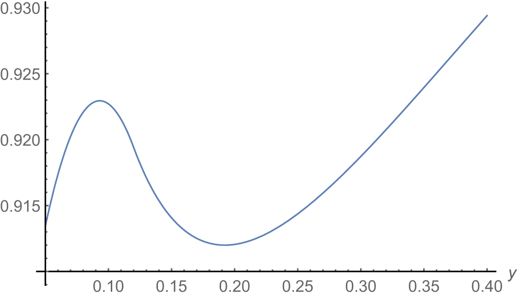


 Open access