


1. Introduction
Two points in a homogeneous and isotropic turbulent flow tend to move apart. As a result, a cloud of Lagrangian tracers spreads under the action of turbulent fluctuations. This fact, known since Taylor (Reference Taylor1922) and Richardson (Reference Richardson1926), is often called turbulent diffusion or dispersion and is often modelled using eddy diffusivities representing turbulent fluctuations in much the same way molecular diffusivities represent molecular agitation and thermal fluctuations.
Formally, the above scenario is valid in homogeneous and isotropic flows. In the ‘dynamic’ case of a stratified flow where density differences actively modify the velocity field, the homogeneity and isotropy assumptions break down. Typically, in that case parcels of fluid – and, hence, Lagrangian tracers carried by these parcels – are subject to restoring buoyancy forces. At least in the case where density is not allowed to irreversibly mix, i.e. when the molecular diffusivity of the scalar setting density  $\kappa$ is zero, such buoyancy forces tend to bring parcels back to their initial (equilibrium) position when vertically displaced, even in the presence of turbulent fluctuations that tend to disperse the parcels. In this case, we expect (eddy) diffusion by turbulent motion to be limited and the emergence of a stationary probability distribution describing the restricted spreading of tracers away from their initial position, in the same way that the diffusive spreading of Brownian particles is constrained when subject to confining potential forces.
On the other hand, when  $\kappa \neq 0$, (irreversible) mixing through molecular diffusion alters the density of a vertically perturbed parcel. As a result, the expected equilibrium position of such a parcel dynamically and irreversibly changes as it comes back to rest. The relevant time scale (or mixing time, denoted $t_{M}$ in what follows), after which mixing substantially alters the density of a fluid parcel is primarily controlled by the rate of kinematic deformation of the parcel (and, hence, by gradients in the macroscopic velocity field that stirs it), molecular diffusion coming into play as logarithmic or weak power-law corrections (Villermaux Reference Villermaux2019). As a result, stirring motions increase the rate of mixing (that otherwise would be controlled by the relatively slow molecular diffusion time scale), which itself affects the driving buoyancy forces of the stirring motions (Caulfield Reference Caulfield2021). How is this intricate two-way coupling affecting the dispersion of Lagrangian tracers? Kimura & Herring (Reference Kimura and Herring1996) and Venayagamoorthy & Stretch (Reference Venayagamoorthy and Stretch2006) empirically showed the emergence of a stationary distribution for the vertical displacement of tracers in stratified turbulent flows in the case $\kappa \neq 0$. Lindborg & Brethouwer (Reference Lindborg and Brethouwer2008) analytically showed that the root-mean-square vertical displacement in freely decaying stratified turbulent flows indeed has a finite limit as time increases, and predicted this limit up to a free parameter corresponding to the time-integrated fraction of potential energy that is dissipated. These studies focused on the effect of the stratification on the dispersion of Lagrangian tracers. Here, we focus on the effects of the molecular properties of the flow.
Our goal is to develop a minimal model describing the (stochastic) path of Lagrangian tracers in stratified turbulent flows. As discussed above, in addition to turbulent fluctuations, the dynamics of Lagrangian tracers is affected by restoring buoyancy forces and by mixing. We here model restoring buoyancy forces as a resetting process (Evans & Majumdar Reference Evans and Majumdar2011; Evans, Majumdar & Schehr Reference Evans, Majumdar and Schehr2020) constraining the otherwise diffusive spread of a cloud of tracers. Mixing is modelled as a memory process (Boyer, Evans & Majumdar Reference Boyer, Evans and Majumdar2017). Indeed, as a parcel of fluid with Lagrangian tracers settles towards its equilibrium position, it mixes with the surrounding environment and, hence, keeps track of the density levels seen along its path, emphasising the fact that ‘history matters’ (Villermaux Reference Villermaux2019). Especially, its density will equilibrate with that of the surrounding fluid at mixing time  $t_{M}$, as experimentally shown in Petropoulos et al. (Reference Petropoulos, Caulfield, Meunier and Villermaux2023). As a result, the parcel will tend to equilibrate at the position it had at $t_{M}$.
Various parameters arise when building the model and we constrain them by studying a reduced-order model for the vertical displacement of an elementary (Lagrangian) density structure carrying Lagrangian tracers (similar to the one developed in Petropoulos et al. Reference Petropoulos, Caulfield, Meunier and Villermaux2023). Importantly, the stochastic model arising from this analysis is simple enough so that an analytical study can be conducted. More precisely, we show the emergence of a stationary probability distribution. We derive scalings for the properties of this distribution as a function of the molecular properties of the fluid (via the Prandtl number  $Pr := \nu /\kappa$, where $\nu$ is the kinematic viscosity) as well as the turbulent characteristics of the flow. We compare the theoretical prediction of the model with the numerical data, both from Riley & de Bruyn Kops (Reference Riley and de Bruyn Kops2003) and from new, never previously reported simulations at various $Pr \neq 1$.
Note that one-dimensional stochastic models have been successfully used in the past to reproduce turbulence characteristics in various flows. Notably, Kerstein (Reference Kerstein1999) formulated a concise model for turbulence in buoyancy-driven flows that takes into account the interplay of advection, molecular transport and buoyancy forces using random mappings applied to one-dimensional velocity and density profiles. The random mappings, whose characteristics are controlled by flow energetics, model the effect of turbulent eddies on the velocity and density fields. The philosophy of the model presented here is similar. However, the tools used, and in particular the formulation of the interplay between advection, molecular diffusion and buoyancy forces, based on stochastic resettings, as well as the purpose of this work are different.
The rest of this work is organised as follows. We first present a numerical experiment that shows the emergence of a stationary distribution of Lagrangian tracers’ vertical displacements in freely decaying stratified turbulent flows (§ 2). We then present a model for the vertical displacement of Lagrangian tracers in stratified turbulent flows that aims to describe the emergence of such a stationary distribution (§ 3). We also compare the model's output to the numerical data. We highlight some limitations of the model in § 4. Conclusions are drawn in § 5.
2. Numerical experiment
In this section we present the methodology used throughout the paper. We start by describing the flow examined here. We consider fully resolved (three-dimensional) direct numerical simulations of stably stratified turbulence building on the simulation campaign originally reported by Riley & de Bruyn Kops (Reference Riley and de Bruyn Kops2003). The flow field satisfies the following (dimensionless) Navier–Stokes equations under the Boussinesq approximations:
 \begin{equation} \left. \begin{gathered} \partial_{t}\boldsymbol{u} + \boldsymbol{u}\boldsymbol{\cdot}\boldsymbol{\nabla}\boldsymbol{u} ={-} \boldsymbol{\nabla} p + \frac{1}{Re_{L}}\nabla^{2}\boldsymbol{u} -\left(\frac{2{\rm \pi}}{Fr_{L}}\right)^{2} \rho^{\prime}\hat{\boldsymbol{e}}_{3}, \quad \boldsymbol{\nabla} \boldsymbol{\cdot} \boldsymbol{u} = 0,\\ \partial_{t}\rho^{\prime} + \boldsymbol{u} \boldsymbol{\cdot} \boldsymbol{\nabla} \rho^{\prime} - u_{3} = \frac{1}{Pr Re_{L}}\nabla^{2}\rho^{\prime}. \end{gathered} \right\} \end{equation}
Here  $\hat {\boldsymbol {e}}_{3}$ is the (upward) vertical unit vector, $\rho ^{\prime }$ is the density deviation from a linear background density profile characterised by a buoyancy frequency $N$,
$N$,  $p$ is the pressure perturbation away from hydrostatic balance and $\boldsymbol {u} = (u_{1}, u_{2}, u_{3})$ is the velocity vector. Note that throughout the simulation, the (linear) background density profile is held constant. The dimensionless parameters are: the above-defined Prandtl number $Pr$, the Froude number $Fr_{L} := 2{\rm \pi} U/(NL)$ and the Reynolds number $Re_{L} := UL/\nu$. Here, $U$ and $L$ are characteristic velocity and length scales associated with the initial conditions. The initial velocity field is of the form
 \begin{equation} \boldsymbol{u}(t=0) = U\cos(kx_{3})\left[\cos(kx_{1})\sin(kx_{2}), -\sin(kx_{1})\cos(kx_{2}), 0\right], \end{equation}
corresponding to Taylor–Green vortices ( $(x_{1},x_{2},x_{3})$ is the position vector), where $L := 1/k$ determines the length scale of the initial flow field. A broad-banded noise (with a level of approximately $10\,\%$ of the initial Taylor–Green vortex energy) is added on top of the velocity field (2.2). Note that no density perturbation was initialised so that density fluctuations only appear due to the action of the flow field on the ambient density gradient, taken to be constant initially. No forcing is applied to sustain the turbulence generated by the initial condition and the flow naturally restratifies after the bursting of a turbulent event. In this work, the Froude and Reynolds numbers are fixed to $Fr_{L} = 4$ and $Re_{L} = 3200$ and the Prandtl number varies from $Pr = 1$ to $Pr = 50$. The three simulations considered here are summarised in table 1. Boundary conditions are triply periodic.
Description of the three simulations described in this work.

We define the dissipation rate of turbulent kinetic energy  $\epsilon$ as the volume average of the pointwise local dissipation rate of turbulent kinetic energy, defined in terms of the symmetric part of the strain-rate tensor $s_{ij}$ as (in dimensional form, $\langle {\cdot } \rangle _{V}$ denotes a volume average)
 \begin{equation} \epsilon := \left\langle 2\nu s_{ij} s_{ij}\right\rangle_{V} ; \quad s_{ij} := \frac{1}{2} \left ( \frac{\partial u_i}{\partial x_j}+ \frac{\partial u_j}{\partial x_i} \right). \end{equation}
This quantity appears in the buoyancy Reynolds number  $Re_{b}$, effectively a measure of the intensity of the stratified turbulence, i.e.
 \begin{equation} Re_{b} := \left(\frac{L_{O}}{L_{K}}\right)^{4/3} = \frac{\epsilon}{\nu N^{2}}; \quad L_{K} := \left(\frac{\nu^{3}}{\epsilon}\right)^{1/4}, \quad L_{O} := \left(\frac{\epsilon}{N^{3}}\right)^{1/2}, \end{equation}
where  $L_{K}$ is the Kolmogorov scale and $L_{O}$ the Ozmidov scale. We also define the (dimensional) destruction rate of buoyancy variance $\chi$ as the volume average
 \begin{align} \chi = \left\langle \frac{g^{2}\kappa}{\rho_{0}^{2}N^{2}} \boldsymbol{\nabla} \rho^{\prime} \boldsymbol{\cdot} \boldsymbol{\nabla} \rho^{\prime} \right\rangle_{V}, \end{align}
with  $\rho _{0}$ denoting a reference density and $g$ the acceleration of gravity. Howland, Taylor & Caulfield (Reference Howland, Taylor and Caulfield2021) noted that, scaled in this way (i.e. considering that the appropriately averaged density gradient against which turbulence is acting corresponds to the background density gradient), $\chi$ provides a good approximation to the mean diapycnal mixing rate (and, more precisely, to the destruction rate of available potential energy), even in flows with significant variations in local stratification.
The time evolution of  $Re_{b}$, $\epsilon$, $\chi$ and the turbulent flux coefficient $\varGamma := \chi /\epsilon$ are presented in figure 1. As $Pr$ increases, $\epsilon$ increases, leading to an increase in buoyancy Reynolds number $Re_{b}$. Conversely, $\chi$ decreases and, hence, the flux coefficient decreases. Similar behaviours have been reported for both decaying and forced stratified turbulent flows (Riley, Couchman & de Bruyn Kops Reference Riley, Couchman and de Bruyn Kops2023; Petropoulos et al. Reference Petropoulos, Couchman, Mashayek, de Bruyn Kops and Caulfield2024).
Time evolution of  $Re_{b}$ (a), $\epsilon$ (b), $\chi$ (c) and $\varGamma$ (d) for the three simulations studied in this work.

We are here interested in a Lagrangian description of mixing and ask the following question: How is mixing (of density) and its aforementioned dependence on the Prandtl number affecting the vertical dispersion of Lagrangian tracers? To answer this question,  $32\,000$ Lagrangian particles are released at $t = 7$. The initial positions of the particles are randomly chosen in the simulation domain, determining the density of the parcels of fluid embedding the particles, which can then change subsequently due to (irreversible) diffusive mixing where $\kappa \neq 0$. A second-order Adams–Bashforth scheme is used to advance the particles in time. The time evolution of the three components of the mean square displacement of the particles $\langle \boldsymbol {x}^{2}(t) \rangle$ (defined as the position of the particles at time $t$ minus their initial position) is presented in figure 2 ( $\langle {\cdot } \rangle$ denotes a statistical average). Whereas the horizontal components of the displacements showcase a diffusive behaviour (with eddy diffusivities given by the slope of the mean square displacement curves), the mean and variance of the vertical displacement seem to reach a steady state. This suggests the existence of a stationary probability distribution describing the vertical displacement of Lagrangian particles in decaying stratified turbulence. Note that a similar result was observed by Kimura & Herring (Reference Kimura and Herring1996); see, for instance, Kimura & Herring (Reference Kimura and Herring1996, figure 5). Similar observations were made by Venayagamoorthy & Stretch (Reference Venayagamoorthy and Stretch2006). These two studies focused on the effect of the stratification on the vertical dispersion of Lagrangian particles. Here, we focus on the effect of the molecular properties of the flow. We aim to describe and model the emergence of such a stationary distribution in the next section.
Time evolution of the mean square displacement in (a) the horizontal and vertical directions and (b) the vertical (only) direction. Note the different vertical axes. A straight line is shown in panel (a) to demonstrate the (close to) diffusive behaviour in the horizontal. The different colours represent different Prandtl numbers.

3. Description of the model
3.1. Model without diffusion and a frozen density field
Let us first briefly consider the case without diffusion of density (i.e.  $\kappa = 0$ or equivalently $Pr \rightarrow +\infty$). In that case, the density field is advected by the velocity field and, hence, the density carried by a Lagrangian parcel of fluid is constant in time. As a result, one could assume that a Lagrangian parcel in a linearly stratified turbulent flow is subject to Brownian motion in a quadratic potential (modelling the buoyancy forces on this parcel of constant density) provided that the background density profile that the parcel is exploring is and stays linear. Such dynamics admit a stationary state described by a Gaussian distribution. This method has however some drawbacks. It assumes that the density levels that the parcel sees on its stochastic path correspond to the density levels of the initial linear density profile, i.e. that the density field is frozen in time. This assumption might break down for vigorously turbulent flows and for $\kappa \neq 0$, i.e. when vigorous stirring and/or mixing obscure the initially linear background density field. Extending the above method to the case $\kappa \neq 0$ also requires the introduction of a model for the time evolution of the density carried by the Lagrangian parcel of fluid. This added complexity might make the analysis relatively complex. In the next section we hence develop a simpler approach, based on stochastic processes subject to resetting.
3.2. Model with diffusion
In this section we model the stochastic trajectories of the Lagrangian parcels of fluid bringing together ideas from stochastic processes subject to resetting (Evans & Majumdar Reference Evans and Majumdar2011) and memory (Boyer et al. Reference Boyer, Evans and Majumdar2017). The main modelling assumption of this work is that buoyancy forces eventually act to collapse a fluid parcel's stochastic trajectory onto the neutrally buoyant position of the parcel. In terms of probabilities, this translates into an increased chance of finding a fluid parcel in the neighbourhood of its neutrally buoyant position after a given (resetting) time.
3.2.1. Stochastic process with resetting
Let us start by considering a tracked parcel of fluid whose vertical position  $z(t)$ is subject to Brownian motion with diffusion coefficient $D$ and is reset to its initial (neutrally buoyant) position $z_{0} = 0$ with a given probability (see pink trajectory on figure 3). The diffusion process models the ambient turbulence whereas the resetting events mimic the restoring effect of stratification in the absence of mixing (i.e. $\kappa = 0$ and, hence, the parcel's density remains constant). For simplicity, we assume that the resetting events follow a Poisson process. Hence, the probability of resetting the parcel between $t$ and $t + \mathrm {d}t$ is equal to $r\mathrm {d}t$ (where $r$ is the resetting rate) and the position of the parcel is updated as (Evans & Majumdar Reference Evans and Majumdar2011)
 \begin{equation} z(t + {\rm d}t) = \begin{cases} z(t) + \xi(t)\sqrt{\mathrm{d}t}, & \text{with probability } 1 - r\,\mathrm{d}t, \\ 0, & \text{with probability } r\,\mathrm{d}t, \end{cases} \end{equation}
where  $\langle \xi (t) \rangle = 0$, $\langle \xi (t)\xi (t') \rangle = 2D \delta (t - t')$ and $\delta$ is the Dirac $\delta$ function. The associated ‘forward master’ equation for the probability $p(z, t)$ of finding a parcel in a neighbourhood of $z$ at time $t$ is
 \begin{equation} \partial_{t}p(z, t) = D\partial_{z}^{2}p(z, t) - rp(z, t) + r\delta(z). \end{equation}
On the right-hand side, the first term expresses the diffusive spread of probability, while the last two terms express the loss of probability of finding the parcel at position  $z$ and the gain of probability of finding it at its neutrally buoyant position, respectively.
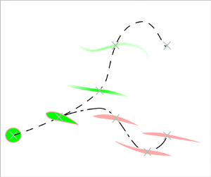
Schematic description of the model for the vertical displacement of Lagrangian particles in stratified turbulent flows, showing the two limiting regimes (i.e. ‘dispersing’ and ‘settling’) discussed in the text. A Lagrangian particle, represented by a grey cross, is initially in a density structure (depicted in green or pink). This structure is kinematically stretched by the flow. This stretching enhances the rate at which the density inside the structure adjusts to that of the surrounding fluid, hence defining a mixing time  $t_{M}$. Because of restoring buoyancy forces, the structure also tends to come back to its initial position on a resetting time scale $t_{R}$. The competing effects of mixing and resetting will influence the equilibrium position of the structure at $t_{R}$ (vertical dotted line). For the green structure, mixing (schematically represented by shades of green) happens before resetting and, hence, the structure comes to equilibrium at the height it has at mixing time, demonstrating the ‘dispersing’ behaviour of moving away from its initial position. For the pink structure, mixing does not have time to happen before resetting and, hence, the structure comes back to its initial position, demonstrating the ‘settling’ behaviour.

Let us now consider mixing. As the parcel moves along its stochastic path, its density changes at a rate that is controlled by the interplay between kinematic stretching and molecular diffusion (Villermaux Reference Villermaux2019). This interplay is modelled through a mixing time  $t_{M}$ at which the density of the parcel starts equilibrating with the density of the surrounding fluid, as shown by Petropoulos et al. (Reference Petropoulos, Caulfield, Meunier and Villermaux2023). Furthermore, the authors showed experimentally that the parcel's position at mixing time $z(t_{M})$ provided a good approximation of its neutrally buoyant position after being mixed. Hence, instead of resetting the parcel's position to its initial position, it is natural to reset it at the position it had at $t_{M}$ (see green trajectory on figure 3). This strategy allows us to bypass the modelling of the time evolution of the ‘background’ density field that the parcel sees on its stochastic path, at least if the density field does not evolve drastically between the mixing and resetting times. The mixing time $t_{M}$ is sampled from the probability density function $\mathcal {T}_{M}(t_{M})$ that we assume to be of exponential form with mean mixing time $\langle t_{M} \rangle$:
 \begin{equation} \mathcal{T}_{M}(t_{M}) = \frac{\exp(t_{M}/\langle t_{M} \rangle)}{\langle t_{M} \rangle}. \end{equation}
Two reasons justify this choice. First, it enables an analytical analysis of the problem. Second, it has been shown to describe accurately the distribution of mixing times for passive scalar mixing in freely decaying turbulence (Duplat, Innocenti & Villermaux Reference Duplat, Innocenti and Villermaux2010). For completeness, we briefly recall their main arguments here. We assume that a fluid parcel carrying a given scalar content experiences successive random stretching of decaying rate but over increasing periods of time, modelling the effect of decaying turbulence. Therefore, the time  $t_{M}$ for this parcel to mix (i.e. for its scalar content to diminish significantly) follows a non-inhomogeneous Poisson process whose last step is the most important, in the sense that the distribution of $t_{M}$ can be well approximated by the distribution of waiting times during the last step of the process. As a result, it is reasonable to assume that $t_{M}$ follows an exponential distribution.
Therefore, (3.2) needs to be modified as follows (Boyer et al. Reference Boyer, Evans and Majumdar2017):
 \begin{equation} \partial_{t}p(z, t) = D\partial_{z}^{2}p(z, t) - rp(z, t) + r\int_{0}^{t}\mathcal{K}(t_{M}, t)p(z, t_{M})\,\mathrm{d}t_{M}. \end{equation}
Here
 \begin{equation} \mathcal{K}(t_{M}, t) := \frac{\mathcal{T}_{M}(t_{M})}{\int_{0}^{t}\mathcal{T}_{M}(\tau)\,\mathrm{d}\tau} \end{equation}
is the truncated version of  $\mathcal {T}_{M}$ between $0$ and $t$, as the parcel cannot be reset to a position it has not yet explored. Note that the resetting time $1/r$ and the mean mixing time $\langle t_{M} \rangle$ are not necessarily equal here; inertia and ambient turbulence potentially allow parcels to overshoot their equilibrium.
The above model (3.4) is however incomplete since it now neglects the restoring action of buoyancy forces for long mixing times. More precisely, if the mixing time is larger than the natural time for the parcel to come back to its initial position in the absence of mixing, then the parcel will in fact come back to its initial position, since its density did not have time to change before the reset. This effect is modelled as follows: if the mixing time associated with a parcel is larger than the waiting time between two resets, it is reset to its initial position. As discussed later in § 4, this is an approximation. Due to the exponential nature of the distribution of times between resets (recall that the resetting process is assumed to be Poissonian) and of mixing times, a resetting event happens with probability  $l$ such that
 \begin{equation} l = \frac{r\langle t_{M} \rangle}{1 + r\langle t_{M} \rangle}. \end{equation}
The overall forward master equation is the weighted linear combination of (3.2) (pink trajectory on figure 3) and (3.4) (green trajectory) with weights  $l$ and $1-l$, respectively:
 \begin{align} \partial_{t}p(z,t) &= \underbrace{D\partial_{z}^{2}p(z,t)}_{\text{Dispersion}} - \underbrace{rlp(z,t) + rl\delta(z)}_{\text{Settling back to initial position}}\nonumber\\ &\quad - \underbrace{r(1-l)p(z,t) + r(1-l)\int_{0}^{t}\mathcal{K}(t_{M}, t)p(z,t_{M})\mathrm{d}t_{M}}_{\text{Memory}}. \end{align}
Interestingly, this equation can be solved analytically and has a stationary solution of the form
 \begin{equation} p_{\infty}(z) = \sum_{m=0}^{+\infty}A_{m}\mathrm{e}^{-\sqrt{({r + m/{\langle t_{M} \rangle}})/{D}}| z |}; \end{equation}
see the Appendix for the derivation and the coefficients  $A_{m}$. We closely follow Boyer et al. (Reference Boyer, Evans and Majumdar2017) who considered the case $l=0$. This stationary distribution behaves as $\mathrm {e}^{-\sqrt {r/{D}}\vert z \vert }$ for large $\vert z \vert$. Hence, this model exhibits a screening length $\sqrt {{D}/{r}}$ that parcels and, hence, Lagrangian tracers will rarely cross. The stationary mean square vertical displacement is
 \begin{equation} \langle z^{2}(t \rightarrow +\infty) \rangle = 4\sum_{m=0}^{+\infty}A_{m}\left[\frac{D}{r + {m}/{\langle t_{M} \rangle}}\right]^{{3}/{2}}. \end{equation}
3.2.2. Physical interpretation
The model presented above (3.7) involves various parameters: the resetting rate  $r$, the mean mixing time $\langle t_{M} \rangle$ and the effective diffusivity of the Lagrangian tracers $D$. Here, we establish connections between these abstract quantities and measurable properties of a real flow. To do so, it is instructive to first think about a simple case. Let us consider a Lagrangian tracer that is embedded into a density structure (a lamella) of initial size $s_{0}$. We assume that the dynamics of the lamella is viscously dominated. The lamella is stretched at a given rate $\gamma$ that determines its mixing time $t_{M} := {\mathcal {F}(Pe)}/{\gamma }$, where the Péclet number $Pe := {\gamma s_{0}^{2}}/{\kappa }$. As a result, its length along the direction of stretching $\ell$ increases with time. The (increasing) function $\mathcal {F}$ is a ‘weak’ diffusive correction that depends on the stretching protocol at hand (Villermaux Reference Villermaux2019). The (vertical) position of the lamella $z_{b}$ has been shown to satisfy the following (dimensionless) equation (see Petropoulos et al. Reference Petropoulos, Caulfield, Meunier and Villermaux2023 for more details):
 \begin{equation} \frac{\mathrm{d}^{2}z_{b}}{\mathrm{d}t^{2}} ={-}\frac{\alpha}{Re}\ell(t)\frac{\mathrm{d}z_{b}}{\mathrm{d}t} - \left(\frac{1}{Fr^{2}\rho_{b}}\right)z_{b} - \beta\left(1 - \frac{1}{\rho_{b}}\right). \end{equation}
Here  $\rho _{b}$ denotes the (maximal) density of the lamella, $\ell$ its length (that increases with time $t$, the functional form of $\ell (t)$ depending on the stirring velocity field) and $\alpha$ is an ${{O}}(1)-{{O}}(10)$ drag coefficient. Time $t$ has been scaled by the shear time ${1}/{\gamma }$, $z_{b}$ by $s_{0}$ and $\rho _{b}$ by the initial (maximal) density of the lamella and, hence, $Re := {\gamma s_{0}^{2}}/{\nu }$, $Fr := {\gamma }/{N}$ and $\beta := {g}/[{s_{0}\gamma ^{2}}]$.
In the viscous regime  $Re \lesssim 1$, the vertical trajectory of the lamella is well approximated by assuming that the density of the lamella $\rho _{b}$ is constant ( $\rho _{b} = 1$ in dimensionless units) before the mixing time and then equal to the density of the surrounding fluid at the position $z_{b}(t_{M})$. If the mixing time is larger than the natural time for the lamella to return to its initial position (without mixing), it ‘settles’ back at its initial position, justifying the resetting strategy presented in the previous section. In the absence of mixing (i.e. $\rho _{b} = 1$ at all times), two important quantities can be inferred. First, considering the balance between friction and buoyancy and neglecting the inertial term (a balance that inevitably happens when $Re \lesssim 1$ and $\ell$ becomes large at late times) the natural (damping) time it takes for the lamella to settle (in the absence of mixing) is of order $\sim {\alpha Fr^{2}}/{(\gamma Re)}$ in dimensional form (Petropoulos et al. Reference Petropoulos, Caulfield, Meunier and Villermaux2023).
Second, considering the oscillatory behaviour due to the (early time) balance between inertia and buoyancy forces, we find that the maximal excursion of the lamella (again, in the absence of mixing) is of order  $\sim {\sqrt {2\mathcal {E}_{k}}Fr}/{\gamma }$ (where $\mathcal {E}_{k}$ is the initial kinetic energy per unit mass of the lamella). Since ${1}/{r}$ corresponds to the natural time it takes for a Lagrangian tracer to come back to its initial position and $\sqrt {{D}/{r}}$ defines the maximum excursion of the tracer, we can therefore infer, in the viscous regime considered here, that
 \begin{equation} r \sim \frac{\gamma Re}{\alpha Fr^{2}}, \quad \sqrt{\frac{D}{r}} \sim \frac{\sqrt{2\mathcal{E}_{k}}Fr}{\gamma}. \end{equation}
We now extend the above reasoning to the turbulent regime. In Petropoulos et al. (Reference Petropoulos, Caulfield, Meunier and Villermaux2023) the size  $s_{0}$ of the lamellae was externally imposed in the experiment. In a turbulent flow, it is reasonable to think that this size, or at least its statistical mean, will emerge as a property of the turbulence. Here, we assume that the lamellae form on scales such that $Re \sim 1$, i.e. scales such that stretching balances viscous dissipation and, more specifically, scales at which vorticity starts to be viscously dissipated so that the kinematics of the lamellae are mainly affected by local strain. Therefore, $s_{0} \sim \sqrt {{\nu }/{\gamma }}$ and $Pe \sim Pr$ (Duplat et al. Reference Duplat, Innocenti and Villermaux2010). Finally, an estimate of the shear rate $\gamma$ is still required. In a turbulent regime, this quantity is statistically distributed. However, recalling that it is defined as the norm of the symmetric part of the strain tensor, the mean shear rate scales as $\sqrt {{\epsilon }/{\nu }}$ (Batchelor Reference Batchelor1959). Therefore,
 \begin{equation} \gamma \sim \sqrt{\frac{\epsilon}{\nu}}, \quad r \sim \frac{\gamma}{\alpha Re_{b}}, \quad \sqrt{\frac{D}{r}} \sim \sqrt{\frac{1}{5}}L_{T}\sqrt{Re_{b}}, \quad \langle t_{M} \rangle = \frac{1}{\gamma}\mathcal{F}(Pr), \end{equation}
and the parameters of the model presented above can therefore be estimated from measurable quantities of the flow and molecular properties of the fluid. The length  $L_{T}$ is the Taylor length scale defined as $L_{T} \simeq \sqrt {10\nu {\mathcal {E}_{k}}/{\epsilon }}$. Equivalently, this can be rephrased as a function of the buoyancy time scale ${1}/{N}$ and $Re_{b}$ as follows:
 \begin{equation} \gamma \sim N\sqrt{Re_{b}}, \quad r \sim \frac{N}{\sqrt{Re_{b}}}, \quad \sqrt{\frac{D}{r}} \sim \sqrt{\frac{1}{5}}L_{T}\sqrt{Re_{b}}. \end{equation}
(We assume  $\alpha$ to be an order ${O}(1)$ quantity here, and in what follows.)
These estimates are presented in figure 4 for the three simulations. Note that the screening length  $\sqrt {{D}/{r}}$ varies like ${1}/{N}$ and, hence, we expect that the mean squared vertical displacement of the particles varies as $N^{-2}$ (a scaling confirmed in figure 5b), as suggested empirically by Kimura & Herring (Reference Kimura and Herring1996) and Venayagamoorthy & Stretch (Reference Venayagamoorthy and Stretch2006) and derived theoretically by Lindborg & Brethouwer (Reference Lindborg and Brethouwer2008) in the case of freely decaying stratified turbulence.
Parameters inferred from the scaling laws (3.11a,b): (a) shear time scale  $\gamma ^{-1}$, (b) resetting rate $r$, (c) eddy diffusivity $D$, (d) screening length $\sqrt {{D}/{r}}$.

(a) Mean square displacement  $\langle z^{2} \rangle$ of the stationary probability distribution $p_{\infty }(z)$ solution of (3.7) as a function of $r\langle t_{M} \rangle$, highlighting the differences between the ‘dispersive’ and ‘settling’ regimes discussed in the text. (d) The probability distribution $p_{\infty }$ in the regime $r\langle t_{M} \rangle \ll 1$ for various values of the mean mixing time $\langle t_{M} \rangle$ (the inset corresponds to the same figure in log-linear coordinates). As $\langle t_{M} \rangle$ increases, extreme events are (slightly) favoured. (e) The analogous plots to panel (d) in the regime $r\langle t_{M} \rangle \gg 1$ for various values of $\langle t_{M} \rangle$. As $\langle t_{M} \rangle$ increases, extreme displacements are prevented and the particles cluster around $z=0$, i.e. no net displacement is favoured. Note that in order to ensure that the screening length $\sqrt {{D}/{r}}$ is always constant, $r=0.1$ and $D=10^{-4}$. (b–c) Mean square displacement $\langle z^{2} \rangle$ as a function of $N$ (b) or $Pr$ (c) (all other parameters being fixed; here $\epsilon = 1$, $L_{T} = 1$ and $\nu = 1$).

3.2.3. Limit cases
In the model presented above (3.7), the product  $r\langle t_{M} \rangle$ plays a key role; it controls the ratio ${l}/{(1 - l)}$ and, hence, the importance of the resetting term relative to the memory term.
Let us first consider the case  $r\langle t_{M} \rangle \gg 1$. We refer to this regime as the ‘settling’ regime. If the mean time between resets ${1}/{r}$ is small compared with the mean mixing time $\langle t_{M} \rangle$, statistically mixing does not have time to happen between resets and the particles (for which the density of the structures that carry them does not have time to change) will favourably be reset to their initial position and so ‘settle’ (back). As $\langle t_{M} \rangle$ increases, the condition $r\langle t_{M} \rangle \gg 1$ becomes stronger and the statistics of mixing times shift towards large values; we then expect more particles to settle back to their initial position before mixing and, hence, the probability distribution $p_{\infty }(z)$ to be more peaked around $z=0$. In terms of the physical parameters of the problem, the condition $r\langle t_{M} \rangle \gg 1$ can be rephrased as ${\mathcal {F}(Pr)}/{Re_{b}} \gg 1$, i.e. the flow is in the settling regime. In that regime, the above-listed aspects suggest that as $Pr$ increases (and, hence, $\langle t_{M} \rangle$ increases), more particles cluster around $z=0$.
Let us now consider the case  $r\langle t_{M} \rangle \ll 1$, which we refer to as the ‘dispersive’ regime. In that regime, the mean time between resets ${1}/{r}$ is large compared with the mean mixing time $\langle t_{M} \rangle$ and the stochastic dynamics is mainly controlled by the memory term. As the particles evolve on their stochastic paths, they are preferentially reset (when that happens) to the position at their mixing time rather than at their initial position, with mixing having time to occur in between the two resetting events. As a result, as $\langle t_{M} \rangle$ increases (but is still small enough so that $r\langle t_{M} \rangle \ll 1$), we expect particles to travel longer distances in a statistical sense, and so they are likely to ‘disperse’. Indeed, as particles are dispersed away from their initial position by turbulent fluctuations, those with large mixing times (an event that is more likely for large $\langle t_{M} \rangle$) will have time to travel longer distances before mixing. Therefore, they will be reset further away from their initial position compared with particles with small mixing times when reset happens (at the actual position at mixing time). Reformulated in terms of the physical parameters of our problems, this means that in this ‘dispersive’ regime ${\mathcal {F}(Pr)}/{Re_{b}} \ll 1$, as $Pr$ increases (and, hence, $\langle t_{M} \rangle$ increases), we expect – everything else being kept equal – that the particles will statistically travel longer vertical distances, turbulent fluctuations winning over restoring buoyancy forces. In other words, in that regime, since the particles with large mixing times have more time to be dispersed by turbulent fluctuations away from their initial position before mixing, they will be reset further away from their initial position when they start ‘feeling’ the stratification and are reset at the position they had at mixing time.
We can summarise these observations as follows. At a fixed screening length  $\sqrt {{D}/{r}}$, as $r\langle t_{M} \rangle$ increases, we move from a ‘dispersive’ regime where the variance of the stationary process increases to a ‘settling’ (back) regime where the variance decreases, as shown in figure 5. In terms of the physical parameters of the problem, the Prandtl number $Pr$ plays a role (through the weak diffusive correction $\mathcal {F}(Pr)$) in defining the boundary between the ‘dispersive’ and ‘settling’ regimes; for $N$ and $\epsilon$ fixed, there exists a large enough $Pr$ so that the regime is ‘settling’.
3.2.4. Comparison with numerical data
Let us now compare the stationary probability distributions of vertical displacements predicted using (3.8) and the empirically determined distributions from our numerical data. Figure 6 summarises the numerical data and the model predictions for the three simulations considered here. The model parameters used here are  $D \simeq 0.01$, $r \simeq 0.8$ and $\gamma ^{-1} \simeq 0.3$, values that are in relative agreement with the theoretical predictions presented in figure 4, at the time when the turbulence is the most energetic. The weak diffusive correction for the mean mixing times $\langle t_{M} \rangle$ is assumed to be logarithmic, corresponding to exponential stretching (Duplat et al. Reference Duplat, Innocenti and Villermaux2010; Villermaux Reference Villermaux2019). This seems to be a reasonable choice in stratified turbulence where fluid parcels are elongated at an exponential rate in the two horizontal directions. The model's prediction seems to fit the data relatively well, the main discrepancies coming from the small displacement data $z \simeq 0$.
Stationary probability distribution of vertical displacement  $p_{\infty }(z)$ for the simulation data (dots) and the model (3.7) (coloured lines) and (3.4) (black lines). The vertical axis is presented in both linear (panel a) and logarithmic (panel b) scales. A zoom on the $z \simeq 0$ region is presented in panel (c). Dotted lines correspond to $Pr=7$ and dashed lines correspond to $Pr=50$. The inset in panel (a) shows the logarithm of the right tail of the stationary distribution, plotted in log coordinates. Our model predicts a purely exponential tail, a prediction that seems consistent with the data. For reference, we also plot a line with slope $2$, corresponding to a Gaussian tail, e.g. arising when considering a Brownian process in a quadratic potential.

The following trends are observed. As  $Pr$ increases from $Pr=1$ to $Pr=7$, smaller displacements are favoured, whereas from $Pr=7$ to $Pr=50$, larger displacements are more likely. A tentative explanation is given here, since, unfortunately, not only $Pr$ changes but also $\epsilon$, making any comparative analysis challenging. As the Prandtl number $Pr$ increases, $\mathcal {F}(Pr)$ as well as the dissipation rate of turbulent $\epsilon$ increases. Increasing $\mathcal {F}(Pr)$ tends to increase the mean mixing time $\langle t_{M} \rangle$, hence allowing particles to travel longer vertical distances in the ‘dispersive’ regime, as described in § 3.2.3 and considered here, everything else being fixed. Conversely, increasing $\epsilon$ tends to decrease $\langle t_{M} \rangle$, thus preventing particles from travelling long distances. Further complicating interpretation, an increase in $\epsilon$ also tends to decrease the resetting rate $r$ and, hence, potentially allows particles to travel further (at fixed $\langle t_{M} \rangle$). In summary, in the regime considered here, turbulent energetics ( $\epsilon$) and the molecular properties of the fluid ( $Pr$) have competing effects on dispersion. Note also that the eddy diffusivity $D$ (slightly) decreases, a decrease that compensates for the decrease of $r$ so that the screening length $\sqrt {{D}/{r}}$ remains constant, as shown in figure 4(d). Therefore, diffusion by turbulent fluctuations is more limited in the case $Pr=7$ than in the case $Pr=1$. In other words, we are here witnessing the opposite effects of turbulence energetics on mixing times and resetting rates (increasing $\epsilon$ and, hence, $Re_{b}$ decreases the mean mixing time, allowing particles to travel shorter vertical distances in the ‘dispersing’ regime considered here, but increases the mean time between resets $1/r$, allowing particles to travel longer distances). The story is made even more complex by the fact that $r\langle t_{M} \rangle$ is ${O}(1)$ rather than in one of the limit cases studied earlier (§ 3.2.3). Hence, the regime studied here is in fact in the transition between the ‘settling’ regime and the ‘dispersive’ regime described in § 3.2.3. All in all, between $Pr=1$ and $Pr=7$, increases in $Pr$ and $\epsilon$ lead to particles travelling less in the $Pr=7$ case. When $Pr$ increases from $Pr=7$ to $Pr=50$, $\epsilon$ is relatively constant and, hence, the mixing time increases due essentially to changes in $Pr$ with the other parameters remaining approximately constant. As a result, in the marginal case studied here, particles travel longer distances in the $Pr=50$ case in comparison with the $Pr=7$ case.
4. Comments on the model
In this section we discuss the different assumptions used to build the model presented above.
4.1. Distribution of resetting times
The main assumption concerns the distribution of resetting events and mixing times. Resetting (or settling) events are assumed to follow a Poisson process with parameter  $r$. More generally, we could have defined the resetting process through a waiting time distribution between resetting events (Eule & Metzger Reference Eule and Metzger2016). However, it then becomes difficult to write down a forward master equation as one must keep track of the time since the last reset. Since the resetting events are introduced to mimic the restoring forces experienced by particles due to density differences, a perhaps better model would consider the waiting time between two passages at the minimum potential energy level of a particle subject to Brownian motion in a quadratic potential. For the sake of simplicity and analytical solvability, we restricted ourselves to the well-studied Poissonian resetting case. This can perhaps explain the discrepancy between the model and the data around $z=0$, and especially the Gaussian-like distribution near the origin rather than exponential-like distribution as predicted by the model.
4.2. Resetting strategy
On a similar note, we have assumed that if the mixing time associated with a particle is larger than the waiting time between two resets, then the particle should be reset to its initial position, i.e. it should ‘settle’ back. This is an oversimplification; indeed, it would then in fact be more accurate to reset the particle to the position it had at last reset, i.e. its last equilibrium position. This involves keeping track of the resetting times. In the case of Poissonian resetting, this might be possible, since the number of resets up to time  $t$ follows a Poisson distribution and the time of the $n$th reset follows a gamma distribution, but adds significant complexity to the model.
We could, for instance, change the term  $rl\delta (z)$ in (3.7) into
 \begin{equation} r\left[l P(R(t) = 0)\delta(z) + \sum_{n=1}^{+\infty}l_{n}P(R(t) = n)\int_{0}^{t}\mathcal{K}_{r}(t_{r}, t; n, r)p(z, t_{r})\,\mathrm{d}t_{r}\right], \end{equation}
with  $R(t)$ the number of resets up to time $t$, following a Poisson distribution of parameter $rt$, where $\mathcal {K}_{r}(t_{r}, t; n, r)$ is the truncated distribution of the $n$th reset time between times $0$ and $t$ (recall that the $n$th reset time follows a gamma distribution of parameter $n$,
$n$,  $r$) and $l_{n}$ is the probability of the $n$th resetting time being smaller than the mixing time. The other terms in (3.7) should also be changed accordingly, i.e. weighted by $l_{n}P(R(t) = n)$ or $(1-l_{n})P(R(t) = n)$. Compared with the $rl\delta (z)$ resetting term, (4.1) does not enforce the particles to settle back to their initial position $z=0$ and, hence, might correct the discrepancies between the predictions of (3.7) and the simulation data for small displacement $z \simeq 0$. Indeed, as a rule of thumb, the first correction in (4.1) is of the form $P(R(t) = 0)\delta (z) = \mathrm {e}^{-rt}\delta (z)$ and, hence, the particles lose memory of their initial position on a time scale $1/r$. It is therefore instructive to compare the stationary solutions of models (3.7) and (3.4), i.e. the models with or without memory of the initial position, respectively, with the data. As can be seen in figure 6, the data are indeed (slightly) better fitted when considering the stationary solution of (3.4), giving good hope that the full correction (4.1) corrects the model for small displacement $z$. However, this correction prevents any analytical treatment and we therefore limit ourselves here to what is effectively the first step of the (resetting) Poisson process. Such added complexity might (for example) be needed in the case of forced turbulence, which is beyond the scope of this work.
Another important question is whether the resetting term in our model is suitable for modelling the effect of buoyancy force. Note that we are here working with the stochastic paths of the fluid parcels rather than their physical paths and, hence, it seems reasonable to think that restoring buoyancy forces will eventually (i.e. at a randomly sampled resetting time) collapse the fluid parcels’ stochastic paths onto their neutrally buoyant positions. This plausible argument motivated our modelling assumptions.
4.3. Mixing as a single-step Poisson process
Here, we have modelled mixing as a single-step process or, more precisely, as one step in a Poisson process. One could consider more involved multistep processes for which a parcel of fluid can mix, i.e. adjust its density towards that of the surrounding fluid, many times before being reset, especially in the case  ${1}/{r} \gg \langle t_{M} \rangle$. In that case, the ‘settling’ and ‘memory’ terms of (3.7) can be replaced, for instance, by the more complex terms
 \begin{gather} -rp(z,t) \!+\!
r\left[P(M(t)\!=\!0)\delta(x) \!+\! \sum_{n=1}^{+\infty}P(M(t) \!=\!
n)\int_{0}^{t}\mathcal{K}_{M}(t_{M}, t;n,{1}/{\langle t_{M}
\rangle})p(z, t_{M})\,\mathrm{d}t_{M}\right],
\end{gather}
\begin{gather} -rp(z,t) \!+\!
r\left[P(M(t)\!=\!0)\delta(x) \!+\! \sum_{n=1}^{+\infty}P(M(t) \!=\!
n)\int_{0}^{t}\mathcal{K}_{M}(t_{M}, t;n,{1}/{\langle t_{M}
\rangle})p(z, t_{M})\,\mathrm{d}t_{M}\right],
\end{gather}
where  $M(t)$ is the (stochastic) number of mixing events encountered by the parcel up to time $t$,
$t$,  $\mathcal {K}_{M}(t_{M},t;n,{1}/{\langle t_{M} \rangle })$ is the truncated distribution of the $n$th mixing time, respectively Poisson and gamma distributed if one assumes that mixing events follow a Poisson process. For the sake of simplicity and analytic resolution, we restricted ourselves to the first term of the above series.
4.4. Slowly evolving density field
We have constructed our model around the key idea that particles come back to their position at mixing time. There is an underlying assumption to this, namely that the density field does not evolve significantly between the mixing time of the fluid parcel containing the particles and its resetting time: otherwise, the position of the parcel at mixing time might not be its equilibrium position at resetting time. In other words, we have assumed that the density field a fluid parcel explores on its stochastic path is only slowly evolving on time scales of the order  $| t_{M} - {1}/{r} |$. This assumption might well break down in the presence of a high-frequency background internal wave field for instance. To remove this reversible contribution to the evolution of the density field, one could work in sorted density coordinates $z_{\ast }$ instead of physical coordinates $z$ for instance, and especially reset particles in the sorted rather than physical coordinates. However, it is somewhat challenging to interpret the physical meaning of a stochastic path in sorted density coordinates.
5. Discussion
We have developed a model for the dispersion of Lagrangian particles in stably stratified turbulent flows. Whereas the horizontal displacements seem well described by a diffusive process, the vertical displacements arise from the competing effects of an eddy diffusivity that tends to ‘disperse’ particles away from their initial position and restoring buoyancy forces that tend to cause the particles to ‘settle’ back towards their initial positions. These competing effects allow the statistics of vertical displacements to reach a stationary distribution, as suggested by Kimura & Herring (Reference Kimura and Herring1996) and Venayagamoorthy & Stretch (Reference Venayagamoorthy and Stretch2006).
Our model is built around the following ideas. Lagrangian tracers are embedded into density structures or ‘lamellae’ that are energised by turbulent fluctuations. Simultaneously, restoring buoyancy forces tend to dampen the dynamics of the ‘lamellae’ by bringing them back to equilibrium positions that depend on their integrated mixing history. Turbulent fluctuations are modelled as a diffusive process that disperses lamellae. Restoring forces are modelled as a resetting stochastic process that causes the particles to settle back to their initial locations. Mixing of density, that influences the velocity field dispersing the particles, is introduced in the model via a memory term. This term keeps track of the position explored by the lamellae (and the Lagrangian particles that they carry) along their stochastic paths and takes into account the fact that the equilibrium position of a lamella dynamically changes as a consequence of mixing of the density field and is determined by its position at mixing time, as shown experimentally by Petropoulos et al. (Reference Petropoulos, Caulfield, Meunier and Villermaux2023).
The different parameters of the model are constrained through the study of a reduced-order model for the vertical displacement of an elementary (Lagrangian) density structure (a lamella) carrying the Lagrangian particles. Importantly, this allowed us to find scaling laws for the different parameters of the model as functions of measurable bulk quantities of the flow; namely measures of the stratification, turbulent kinetic energy and its dissipation rate and the molecular properties of the scalar being mixed. To our knowledge, this is the first attempt to describe dispersion in stratified turbulent flows without free parameters. Many simplifying assumptions have been made, but the overall reasonable agreement between the model's output and the numerical data considered in this work is encouraging. We certainly do not claim that we have solved the problem of dispersion in stratified turbulent flows but rather showed how simple ideas about the intricate coupling between buoyancy and mixing in such flows can be taken into account and incorporated in a simple (toy) model to gain insight into this complex problem. Especially, we hope that the model is flexible enough to stimulate discussion.
Importantly, our model is simple enough so that it can be solved analytically. A stationary probability distribution emerges from the proposed model. The width of this distribution, characterising a length scale that particles are unlikely to cross, is primarily controlled by the buoyancy Reynolds number  $Re_{b}$ and is (weakly) modulated by the molecular Prandtl number $Pr$. More precisely, in the ‘dispersive’ regime $r\langle t_{M} \rangle \ll 1$ described in § 3.2.3, as $Pr$ increases and, hence, $\langle t_{M} \rangle$ increases, particles are allowed to travel (slightly) longer distances. Indeed, in this regime where buoyancy restoring forces play a secondary role compared with turbulent fluctuations, particles with large mixing times are more likely to travel longer distances before the density structure in which they are embedded mixes with the surrounding fluid and subsequently settles, at least according to the single-step mixing process considered here; see the discussion in § 3.2.3. Conversely, in the ‘settling’ regime $r\langle t_{M} \rangle \gg 1$, buoyancy forces are now playing a critical role as the mean resetting time ${1}/{r}$ is small compared with the mean mixing time, and hence, density structures do not have time to mix before a resetting event. Particles are then preferentially reset to their initial position, to which they ‘settle’ (back). As $Pr$ increases and mixing becomes less efficient, this phenomenon becomes more dominant and particles are less likely to travel long distances.
Note that the above discussion holds when the molecular Prandtl number  $Pr$ alone is varied, everything else being held constant. In practice, changes in $Pr$ have an impact on the buoyancy Reynolds number $Re_{b}$. As $Pr$ increases, $\epsilon$ and, hence, $Re_{b}$ increases (see figure 1). As a result, mixing times decrease, preventing particles from travelling long distances in the ‘dispersive’ regime, but the screening lengths increase. In other words, we witness here the complex and intricate effects of increasing $Pr$ on the vertical displacement of particles. Increasing $Pr$ makes the turbulence more energetic, hence reducing mixing times through the $1/{\gamma } \propto {1}/{\sqrt {Re_{b}}}$ term while still diffusing particles more ‘vigorously’. Conversely, increasing $Pr$ makes the mixing less efficient by increasing mixing times through the weak diffusive correction $\mathcal {F}(Pr)$.
We believe it is appropriate to mention some future directions and open questions. An important assumption of our work is that the Lagrangian tracers themselves do not diffuse since their associated ‘molecular’ diffusivity  $\kappa _{tracer}$ is formally $0$. How should the model be modified to account for the potential intrinsic diffusivity of marked tracers? This could potentially offer insight into how dye, nutrient and climatically relevant tracers such as carbon (three tracers for which it seems reasonable to assume that they passively follow the flow while diffusing at a rate controlled by their associated ‘molecular’ diffusivity) disperse in stratified turbulent flows. This might lead to an important insight into interpreting tracer release experiments (Ledwell, Watson & Law Reference Ledwell, Watson and Law1993) for example. The need to understand the case $\kappa _{tracer} \neq 0$ is exacerbated by the fact that the tracer's mixing time, formally taken to be infinite in this study, is primarily controlled by the inverse shear rate $\gamma \sim \sqrt {{\epsilon }/{\nu }}$, diffusive corrections being usually weak (typically logarithmic). Hence, even a relatively small but non-zero diffusivity of the tracer might drastically impact our modelling assumptions. Similarly, whether resetting processes can be used to interpret vertical distributions of buoyant particles, such as plastic in the ocean, is an interesting avenue of research. For instance, the observed exponential distribution of buoyant plastic debris in the ocean surface boundary layer (Kukulka et al. Reference Kukulka, Proskurowski, Morét-Ferguson, Meyer and Law2012) is consistent with a balance between turbulent dispersion and resetting at the surface due to buoyancy.
Similarly, we neglected in this work the relatively large-scale organisation of the flow (and especially its inherent anisotropy and inhomogeneity) that is thought to arise inevitably in the so-called ‘strongly stratified turbulence’ or, more specifically, the ‘layered anisotropic stratified turbulence’ regime (Brethouwer et al. Reference Brethouwer, Billant, Lindborg and Chomaz2007; Falder, White & Caulfield Reference Falder, White and Caulfield2016; Petropoulos et al. Reference Petropoulos, Couchman, Mashayek, de Bruyn Kops and Caulfield2024). Indeed, we considered bulk-averaged turbulent statistics as meaningful measures of the turbulence at hand. Is this assumption always valid, especially as we increase the Froude number  $Fr_{L}$? If not, what is the most suitable model? We believe that our model can still be used in this setting, at least locally, provided relevant measures of the different parameters of the model, and especially of the background stratification $N$, are considered. In the well-mixed regions of a layered density ‘staircase’, $N$ is relatively low and, hence, the resetting rate $r$ (recall that $r$ was found to be an increasing function of $N$) is small and the density structures effectively do not feel stratification. On the other hand, in the more strongly stratified interfaces, $N$ is relatively large and so is the resetting rate $r$ and so density structures are not allowed to travel long vertical distances between resets (they are ‘trapped’).
We conclude this section with some further comments on the usefulness of the model presented here to probe mixing. By comparing the final and initial positions of a Lagrangian parcel of fluid (and assuming both that these positions correspond to neutrally buoyant positions and that the initial and final background density profiles are known), we can infer the overall (time-integrated) density change of the parcel and, therefore, the amount of mixing it experienced. This is in itself a useful measure of mixing. However, if one wants to dig into the details of the energetics of mixing, the full history of  $p(z, t)$ is needed, as noted by Caulfield (Reference Caulfield2021). We believe that our model, because of its simplicity, might give insight into this time evolution, as we demonstrate using a simple thought experiment. For the simulations considered here, the initial and final background density fields are almost identical regardless of the Prandtl number $Pr$ (see figure 7a) and the final vertical distributions of the Lagrangian parcels are only slightly different, suggesting that fluid elements have experienced the same amount of (time-integrated) density changes between the onset of turbulence and its end when the density field restratifies to the background density profile. However, in the ‘dispersive’ regime considered here (in the sense of § 3.2.3), mixing happens at a slower rate as $Pr$ increases and the associated instantaneous ‘mixing efficiency’ – well approximated by ${\varGamma }/{(1 + \varGamma )}$ (Howland et al. Reference Howland, Taylor and Caulfield2021) – decreases; see figure 1. To resolve this potential (semantic) paradox, one needs to remember the truism that ‘history matters’ when defining mixing (Villermaux Reference Villermaux2019; Caulfield Reference Caulfield2021).
(a) Horizontally averaged density profiles (symbols) at the end of the simulations for various Prandtl numbers. The initial background density profile is depicted in black. (b,c) Climbing a density profile  $\bar {\rho }(z)$ in one (b) or two (c) steps.

Let us consider the following thought experiment: a parcel is climbing a density profile  $\bar {\rho }(z)$ from $z_{0}$ to $z_{f}$ as depicted in figure 7. In the first case (case 1) it climbs the gradient in one step, corresponding to a high-Prandtl-number case, the parcel having more time to climb before mixing since large mixing times are favoured. In the second case it climbs in two steps, corresponding to a low-Prandtl-number case. Whereas the change in background potential energy (per unit volume) is identical in both cases (and equal to $g[\bar {\rho }(z_{f})z_{f} - \bar {\rho }(z_{0})z_{0}]$), the available potential energy (per unit volume) that is injected in the system is $g\bar {\rho }(z_{0})[z_{f} - z_{0}]$ in the first case and $g\bar {\rho }(z_{0})[z_{f,1} - z_{0}] + g\bar {\rho }(z_{f,1})[z_{f} - z_{f,1}] \leq g\bar {\rho }(z_{0})[z_{f} - z_{0}]$ in the second. Therefore, whereas the overall parcel's density change is identical in cases $1$ and $2$, the time-integrated or cumulative mixing efficiency, defined here as the ratio of change in background and available potential energy, is smaller in case $1$ than in case $2$, since a greater amount of energy has to be input in the system to achieve the same change in background potential energy. In a nutshell, we can expect that in the ‘dispersive’ case described in § 3.2.3, as the Prandtl number $Pr$ increases (everything else being held fixed), extreme vertical displacements are favoured because mixing happens at a slower rate, potentially enabling extreme changes in fluid parcels’ density between the onset of turbulence and restratification. However, such extreme displacement comes at a greater energy cost, reducing the cumulative (time-integrated) mixing efficiency. This example shows how mixing (i.e. irreversible changes in the density of a parcel of fluid), (energetic) mixing efficiency and dispersion are not necessarily related and emphasises again that history really matters when considering mixing.
Funding
This project received funding from the European Union's Horizon 2020 research and innovation program under the Marie Sklodowska-Curie Grant agreement no. 956457 and used resources of the Oak Ridge Leadership Computing Facility at the Oak Ridge National Laboratory, supported by the Office of Science of the U.S. Department of Energy under contract no. DE-AC05-00OR22725. S.M.d.B.K. was supported under U.S. Office of Naval Research Grant number N00014-19-1-2152.
Declaration of interests
The authors report no conflict of interest.
Appendix. Analytic solution of the forward master equation
In this appendix we derive the solution to the forward master equation (3.7) with initial condition  $p(z, t=0) = \delta (z)$. Our derivation closely follows the one from Boyer et al. (Reference Boyer, Evans and Majumdar2017) that considered the case $l=0$. More precisely, taking the Fourier transform (in space) of (3.7), differentiating with respect to time and making the change of variable $\hat {p}(k, t) = W(y = \mathrm {e}^{-\lambda t})$ (where $\hat {p}(k, t)$ is the Fourier transform of $p(z, t)$ and $\lambda := {1}/{\langle t_{M} \rangle }$), one obtains the following differential equation for $W$:
$W$:
 \begin{equation} y(1-y)\frac{\mathrm{d}^{2}W}{\mathrm{d} y^{2}}(y) + [c - (a+b+1)y]\frac{\mathrm{d}W}{\mathrm{d}y}(y) - abW(y) = \frac{rl}{\lambda}. \end{equation}
Here
 \begin{equation} ab ={-}\frac{r + k^{2}D - r(1-l)}{\lambda}, \quad c := a + b = 1 - \frac{r + k^{2}D}{\lambda}. \end{equation}
As a result,  $W$ can be expressed in terms of the hypergeometric function $F$, i.e.
 \begin{equation} W(y) = AF(a,b,c;y) + By^{1-c}F(1+a-c,1+b-c,2-c,y) - \frac{rl}{\lambda ab}, \end{equation}
where  $A$ and $B$ constrain the initial condition $W(y=1) = 1$. Exactly as in Boyer et al. (Reference Boyer, Evans and Majumdar2017), we can show that
 \begin{equation} A = \frac{\left (1 + \dfrac{rl}{\lambda ab} \right ) \varGamma(1-a-b)}{\varGamma(1-a)\varGamma(1-b)}, \quad B ={-}A \frac{\varGamma(a+b)\varGamma(1-a)\varGamma(1-b)}{\varGamma(a)\varGamma(b)\varGamma(2-a-b)}. \end{equation}
Here  $\varGamma$ is the gamma function. Since we are interested in the steady state, we take the limit $t \rightarrow +\infty$ and get
 \begin{equation} \hat{p}_{\infty}(k) := \hat{p}(k, t \rightarrow +\infty) = A - \frac{rl}{\lambda ab}. \end{equation}
Since  $A$ has poles at integer values of $1-a-b$ and at $ab = 0$, we have, by inverse Fourier transform,
 \begin{align} p_{\infty}(z) &= \sum_{m=0}^{+\infty}\underbrace{A_{m}\mathrm{e}^{-\sqrt{({r+m\lambda})/{D}}| z |}}_{\text{Pole } 1-a-b=m} - \underbrace{\frac{\sqrt{rl}}{2\sqrt{D}}\mathrm{e}^{-\sqrt{{rl}/{D}}| z |}}_{\text{Pole } ab = 0} + \underbrace{\frac{\sqrt{rl}}{2\sqrt{D}}\mathrm{e}^{-\sqrt{{rl}/{D}}| z |}}_{\text{Inverse Fourier transform of } -\frac{r}{\lambda ab}} \end{align}
 \begin{align} &= \sum_{m=0}^{+\infty}A_{m}\mathrm{e}^{-\sqrt{({r+m\lambda})/{D}}\vert z \vert}, \end{align}
with
 \begin{gather} A_{m} := \left(1 + \frac{rl}{m\lambda + r(1-l)}\right)\frac{1}{2{\rm \pi}}\frac{\lambda}{\sqrt{D(m\lambda + r)}}\frac{(1-a_{m})_{m}}{m!}\sin({\rm \pi} a_{m}), \end{gather}
 \begin{gather}a_{m} := \frac{1}{2}\left[(1 + m) + \sqrt{(1-m)^{2} - 4\frac{r(1-l)}{\lambda}}\right] \end{gather}
and  $(d)_{m} = d(d+1)\cdots (d+n-1)$.


 Open access