





1. Introduction
Cavitation bubbles commonly appear in hydraulic machinery such as pumps and turbines (Arndt Reference Arndt1981; Cristofaro et al. Reference Cristofaro, Edelbauer, Koukouvinis and Gavaises2020; Balz et al. Reference Balz, Nagy, Weisser and Sedarsky2021). Their collapse near solid surfaces can produce extremely high local pressures, intense microjets and pressure waves, leading to severe mechanical and structural damage. Harrison (Reference Harrison1952) provided one of the first experimental measurements of single bubble collapse, showing that shock pressures can reach tens of megapascals, sufficient to damage nearby metal surfaces. Karimi & Martin (Reference Karimi and Martin1986) demonstrated that repeated bubble collapse can erode metal surfaces at rates of up to several micrometres per hour under controlled laboratory conditions, forming pits that coalesce into large-scale material loss. Lauterborn & Kurz (Reference Lauterborn and Kurz2010) quantified that single bubble collapse can produce audible acoustic transients capable of exciting structural resonances. Laguna-Camacho et al. (Reference Laguna-Camacho, Lewis, Vite-Torres and Méndez-Méndez2013) further showed that even small differences in material hardness or microstructure can result in dramatically different erosion rates, highlighting the vulnerability of engineering alloys to cavitation. In addition to material erosion, bubble collapse generates strong pressure pulses and high-frequency noise. Li et al. (Reference Li, Feng, Li, Si and Zhu2018) experimentally confirmed that such pressure fluctuations can induce vibrations large enough to compromise pump and turbine performance, accelerate fatigue and increase maintenance costs. Despite these harmful effects, cavitation bubble collapse can also offer benefits when properly controlled. Gensheng et al. (Reference Gensheng, Zhonghou, Changshan, Debin and Hongbing2005) demonstrated experimentally that controlled bubble collapse near rock surfaces enhances drilling efficiency by generating localised high-pressure pulses that fragment rock without mechanical contact. Maeda et al. (Reference Maeda, Colonius, Kreider, Maxwell and Bailey2016) developed numerical models to optimise bubble-induced pressure pulses in petroleum wells, showing that tuning bubble size and collapse timing can significantly improve penetration rates while minimising unintended erosion. In ultrasonic cleaning applications, Reuter et al. (Reference Reuter, Lauterborn, Mettin and Lauterborn2017) quantified how an acoustic cavitation bubble removes membrane fouling and surface contaminants, demonstrating that collapse-induced microjets and pressure waves can effectively dislodge adhered particles without damaging underlying surfaces. In the background of surface engineering, Soyama, Chighizola & Hill (Reference Soyama, Chighizola and Hill2021) used hydrodynamic cavitation for shotless peening, where repeated controlled bubble collapses produce uniform plastic deformation, improving metal fatigue resistance without mechanical impact or abrasive media. In biomedical contexts, particularly in dentistry, cavitation induced in the cooling water passing over the probe tip has been shown to significantly aid in plaque removal (Walmsley, Laird & Williams Reference Walmsley, Laird and Williams1988).
Whether a cavitation effect is desirable or not, a fundamental understanding of the physics leading to these phenomenons is essential. To this end, focusing on the simplest form of cavitation, the single bubble, enables a controlled investigation of bubble dynamics without the complexity of bubble clouds. Experimental methods have been developed to generate a single vapour bubble on demand. These single bubbles can be generated by several means, most of them not implying a local pressure drop in the liquid, i.e. hydrodynamic cavitation, but by either acoustic waves termed acoustic cavitation or by local energy deposition methods.
Acoustic cavitation occurs when ultrasound waves propagate through the liquid, producing a mechanical vibration that makes the dissolved gas nuclei grow to a bubble (Ashokkumar Reference Ashokkumar2011). The acoustic method excites the bubble over several oscillation cycles and is widely used in the studies of cavitation enhanced chemistry and luminescence. The near-adiabatic collapse of an acoustic cavitation bubble produces extreme local temperatures and pressures, leading to the formation of highly reactive radicals, which initiate a variety of sonochemical processes, including nanomaterial synthesis, polymerisation and degradation of organic pollutants (Mišík & Riesz Reference Mišík and Riesz1996; Rae et al. Reference Rae, Ashokkumar, Eulaerts, von Sonntag, Reisse and Grieser2005; Ashokkumar et al. Reference Ashokkumar, Lee, Kentish and Grieser2007). Moreover, acoustic cavitation has shown potential in biomedical applications, including diagnostic and therapeutic ultrasound (Tsochatzidis et al. Reference Tsochatzidis, Guiraud, Wilhelm and Delmas2001; Iida et al. Reference Iida, Ashokkumar, Tuziuti, Kozuka, Yasui, Towata and Lee2010). However, the acoustic-induced cavitation bubble grows from pre-existing nuclei and its collapse is influenced by continuous pressure waves in the surrounding liquid, making precise control of bubble position, size and collapse time challenging. Energy deposition methods complement this by generating a single bubble precisely at the energy focus, whose collapse is driven solely by the liquid pressure. Thanks to these advantages, it is more controlled to investigate the effect of a pressure gradient on the collapse of a single cavitation bubble (Tinguely Reference Tinguely2013).
The two main energy deposition methods used to generate the cavitation bubble in a liquid are the spark-induced and laser-induced methods. In the spark-induced method, two electrodes are immersed in the water and an electric discharge between creates a small plasma channel that rapidly expands into a vapour bubble. This approach has been extensively applied to study bubble dynamics and related physical phenomena. For instance, Avila, Song & Ohl (Reference Avila, Song and Ohl2015) showed that a microjet generated from a spark-induced bubble can penetrate soft material, opening possibilities for painless, needle-free drug delivery. Zhang et al. (Reference Zhang, Cui, Cui and Wang2015) studied large spark-induced bubbles under buoyant conditions, providing insights into underwater explosion dynamics and cavitation-induced structural loading. Cui et al. (Reference Cui, Zhang, Wang and Khoo2018) employed electric discharge to generate a single bubble near ice plates, demonstrating that the resulting collapse can fracture ice and, thus, be exploited for ice-breaking applications. However, since the electrodes are placed directly within the liquid, the bubble typically forms at the electrode tip, leading to unavoidable interactions between the bubble and the electrodes. This configuration can limit control over bubble positioning and reproducibility. In contrast, the laser-induced method is non-intrusive. The laser beam can be focused through an optical system located outside the test chamber. Laser-induced cavitation is thus seen as a more practical and controllable way to create bubbles near a solid wall with minimal disturbance to the surrounding environment (Brujan et al. Reference Brujan, Nahen, Schmidt and Vogel2001; Tomita et al. Reference Tomita, Robinson, Tong and Blake2002; Zwaan et al. Reference Zwaan, Le Gac, Tsuji and Ohl2007), which is what we intend to investigate in this study.
Motivated by this better controllability, a substantial body of experimental investigations have recently employed high-power lasers to induce cavitation bubbles near a solid wall and study the underlying mechanism in detail. Example studies in this regard include identification of the primary sources of pressure at a wall when a single bubble collapses (Zhao & Coutier-Delgosha Reference Zhao and Coutier-Delgosha2023; Subramanian et al. Reference Subramanian, Yang, Romanò and Coutier-Delgosha2026), morphological evolution of the cavitation bubble collapse (Zhang et al. Reference Zhang, Du, Liu, Sun, Yao and Zhong2022), change of residual wall stress with the relative distance between bubble and wall (Ren et al. Reference Ren, He, Tong, Ren, Yuan, Liu, Zuo, Wu, Sui and Wang2016), influence of a particle on the collapsing dynamics near a solid wall, (Zhang et al. Reference Zhang, Xie, Zhang and Du2019), role of the gaseous composition within bubbles on the collapse dynamics (Preso et al. Reference Preso, Fuster, Sieber, Obreschkow and Farhat2024), measurement of temperature (Dular & Coutier-Delgosha Reference Dular and Coutier-Delgosha2013), pressure (Herbert, Balibar & Caupin Reference Herbert, Balibar and Caupin2006; Subramanian et al. Reference Subramanian, Yang, Romanò and Coutier-Delgosha2026) and velocity (Khlifa et al. Reference Khlifa, Coutier-Delgosha, Fuzier, Vabre and Fezzaa2013) in the liquid, as well as the thermodynamic effects on single cavitation bubble dynamics under various ambient temperature conditions (Phan et al. Reference Phan, Kadivar, Nguyen, el Moctar and Park2022a ). Moreover, the influence of the relative wall distance on the damage caused by laser-induced bubble collapse, as well as the effect of boundary roughness on bubble dynamics, has been experimentally investigated. For example, Dular, Požar & Zevnik (Reference Dular2019) quantified the damaged volume of boundary surface produced by the collapse of a laser-induced bubble at stationary conditions for different relative wall distances, and showed that the impact of the microjet is dominant at small values of a relative wall distance, while its influence diminishes as the bubble collapses farther from the boundary. Kadivar et al. (Reference Kadivar, el Moctar, Skoda and Löschner2021) compared the dynamics of a single laser-induced cavitation bubble near a smooth surface and a microstructured riblet surface, demonstrating that the microstructured boundary can efficiently reduce the destructive effects of bubble collapse. Nguyen et al. (Reference Nguyen, Kadivar, Phan, Nguyen, el Moctar and Park2025) investigated the effects of the free surface on the dynamics of a single laser-induced bubble near a rigid boundary, revealing that the presence of a nearby free surface leads to a larger bubble and more violent collapse compared with the case where the bubble is farther from the rigid boundary.
While the evolution of bubble shape can be measured by high-speed optical imaging, and the flow fields in the liquid as well as boundary effects on bubble dynamics can be quantified, experimental techniques have inherent limitations in capturing the transient internal behaviour within the bubble (e.g. distribution of fields). To overcome these constraints, numerical simulations are highly necessary to study laser-induced cavitation, focusing on the physics behind a single bubble near a solid wall.
A key novelty in this work is the use of a new computational model that combines compressible multiphase fluid dynamics with laser radiation and phase transition, capable of capturing the complete lifecycle of a single bubble near a solid boundary, i.e. from the bubble formation to its collapse. In the past, the common approach in bubble dynamics simulations was to simplify the problem by initiating the bubble from rest near a solid wall, that is, with predefined initial conditions for pressure, temperature and velocity at a given bubble size and with uniformly distributed flow fields. This simplification is typically implemented in one of two ways. The first is to start from the maximum radius to focus on the collapse phase. For instance, Fuster & Popinet (Reference Fuster and Popinet2018) proposed an all-Mach semi-implicit scheme in which a single bubble is initialised from rest with a prescribed non-dimensional maximum radius, in order to study collapse dynamics near a solid wall and capture the high-speed jet formation impacting on the wall. This method was later extended by Saade, Lohse & Fuster (Reference Saade, Lohse and Fuster2023) to account for heat transfer between phases and by Yang, Wang & Romanò (Reference Yang, Wang and Romanò2025) to explore a wide parametric space. The second approach is to start from a small nucleus and simulate most of the expansion phase. Following this strategy, Lechner et al. (Reference Lechner, Lauterborn, Koch and Mettin2020) numerically studied the distance dependence of bubble dynamics and its impact on jet formation. Gonzalez-Avila, Denner & Ohl (Reference Gonzalez-Avila, Denner and Ohl2021) conducted the simulation of bubble expansion as a supplement of the experimental measurements and investigated the origin of the wall pressure peak. Bußmann et al. (Reference Bußmann, Riahi, Gökce, Adami, Barcikowski and Adams2023) numerically studied the expansion and collapse dynamics of a single cavitation bubble near a solid wall using a high-resolution sharp-interface level set method, identifying three jetting regimes. Both of these common numerical approaches rely on a major simplification, i.e. the bubble is initialised from rest with a predefined radius and simplified pressure and temperature initial conditions. In reality, cavitation bubbles nucleate through complex processes involving phase transition, intense non-equilibrium thermodynamics, rapid initial growth and a non-zero initial velocity field (Brennen Reference Brennen2014). These key processes are absent in simulations that start from rest with a predefined bubble. That neglects critical initial conditions that govern the early time energy partition between the liquid and vapour phases, determine the initial pressure, temperature and velocity fields, and thus, decide the bubble’s subsequent dynamics. The impact of this simplification on predictive accuracy has been demonstrated in our previous work (Wang, Yang & Romanò Reference Wang, Yang and Romanò2026), where we considered three stand-off ratios. We found that, for the stand-off ratio of 1.82, by explicitly modelling the water breakdown phase yields the best agreement with experimental measurements of maximum wall pressure, with a relative error of only 6 $\,\%$
, compared with 48
$\,\%$
, compared with 48 $\,\%$
when starting from a small nucleus or 66
$\,\%$
when starting from a small nucleus or 66 $\,\%$
from the maximum bubble size. In this work, we thus include the bubble nucleation by coupling the multiphase compressible Euler equations with a laser radiation equation that models the absorption of laser energy by the fluid flow. The algorithms and properties of this method were recently reported by Zhao, Ma & Wang (Reference Zhao, Ma and Wang2023), together with some verification tests presented by Zhao et al. (Reference Zhao, Ma, Chen, Xiang, Zhong and Wang2024). Additional validations of the computational method are summarised by Zhao et al. (Reference Zhao, Ma, Islam, Narkhede and Wang2026), where the collapse of a single spherical bubble in an infinite liquid medium is simulated and compared in detail with experimental data reported by Kröninger et al. (Reference Kröninger, Köhler, Kurz and Lauterborn2010), showing that spherical symmetry is well preserved during collapse. Related to this effort, laser-induced bubble nucleation has also been addressed at the molecular scale using molecular dynamics simulations coupled with analytical laser–liquid interaction models (Rezaee et al. Reference Rezaee, Kadivar and el Moctar2025). However, such approaches are inherently restricted to nanometre spatial scales and ultrashort time scales, whereas the present framework targets millimetre scale bubble dynamics and wall-induced collapse phenomena. Linking it with continuum-scale bubble dynamics analysis is not straightforward.
$\,\%$
from the maximum bubble size. In this work, we thus include the bubble nucleation by coupling the multiphase compressible Euler equations with a laser radiation equation that models the absorption of laser energy by the fluid flow. The algorithms and properties of this method were recently reported by Zhao, Ma & Wang (Reference Zhao, Ma and Wang2023), together with some verification tests presented by Zhao et al. (Reference Zhao, Ma, Chen, Xiang, Zhong and Wang2024). Additional validations of the computational method are summarised by Zhao et al. (Reference Zhao, Ma, Islam, Narkhede and Wang2026), where the collapse of a single spherical bubble in an infinite liquid medium is simulated and compared in detail with experimental data reported by Kröninger et al. (Reference Kröninger, Köhler, Kurz and Lauterborn2010), showing that spherical symmetry is well preserved during collapse. Related to this effort, laser-induced bubble nucleation has also been addressed at the molecular scale using molecular dynamics simulations coupled with analytical laser–liquid interaction models (Rezaee et al. Reference Rezaee, Kadivar and el Moctar2025). However, such approaches are inherently restricted to nanometre spatial scales and ultrashort time scales, whereas the present framework targets millimetre scale bubble dynamics and wall-induced collapse phenomena. Linking it with continuum-scale bubble dynamics analysis is not straightforward.
Another novelty of the current study is that we apply such a method, previously used only for laser-fibre-attached cavitation and a long-pulsed laser (duration $\sim 100 \,\unicode{x03BC}\textrm{s}$
), for the first time to carry out a detailed study on a wall-detached cavitation bubble induced by a short-pulsed laser (duration
$\sim 100 \,\unicode{x03BC}\textrm{s}$
), for the first time to carry out a detailed study on a wall-detached cavitation bubble induced by a short-pulsed laser (duration $\sim 5\rm\, ns$
). To the best of our knowledge, there is currently no unified theory or computational model for cavitation induced by various types of lasers (duration from nanoseconds to milliseconds) while simultaneously addressing the non-uniform temperature distribution inside the bubble. The current study serves as a step towards bridging this gap. The present work explicitly resolves the cavitation inception phase, which determines the initial thermodynamic and velocity fields and strongly influences subsequent collapse dynamics. In contrast to the previous numerical studies where the bubble is initialised with prescribed or assumed initial conditions, the present approach avoids such initialisation artefacts by modelling a nucleation-consistent process. Based on this computational model, we systematically analyse the effects of the stand-off distance on laser-induced bubble dynamics and peak wall pressure, and we provide a more comprehensive and physically grounded understanding of the collapse process by comparing with experimental measurements by Subramanian et al. (Reference Subramanian, Yang, Romanò and Coutier-Delgosha2026).
$\sim 5\rm\, ns$
). To the best of our knowledge, there is currently no unified theory or computational model for cavitation induced by various types of lasers (duration from nanoseconds to milliseconds) while simultaneously addressing the non-uniform temperature distribution inside the bubble. The current study serves as a step towards bridging this gap. The present work explicitly resolves the cavitation inception phase, which determines the initial thermodynamic and velocity fields and strongly influences subsequent collapse dynamics. In contrast to the previous numerical studies where the bubble is initialised with prescribed or assumed initial conditions, the present approach avoids such initialisation artefacts by modelling a nucleation-consistent process. Based on this computational model, we systematically analyse the effects of the stand-off distance on laser-induced bubble dynamics and peak wall pressure, and we provide a more comprehensive and physically grounded understanding of the collapse process by comparing with experimental measurements by Subramanian et al. (Reference Subramanian, Yang, Romanò and Coutier-Delgosha2026).
The paper is organised as follows: § 2 details the governing equations and problem formulation for laser-induced cavitation bubble; § 3 outlines the numerical methodology and presents the convergence study; § 4 validates the model through the comparison with experimental measurements on interfacial dynamics and peak wall pressure; § 5 compares the three collapse regimes identified in both simulations and experiments; § 6 analyses the bubble dynamics for three selected stand-off ratios; § 7 examines the internal bubble dynamics, including temperature, pressure, velocity and density. Finally, we present the conclusion and future outlook.
2. Problem formulation
2.1. Problem description
In the experiment performed by Subramanian et al. (Reference Subramanian, Yang, Romanò and Coutier-Delgosha2026), a Q-switched Nd: YAG laser (Big Sky Laser PN00148300) with a wavelength of 532 nm, maximum pulse energy of 200 mJ and a pulse duration of 5 ns was used as the energy source to induce the cavitation bubble. The experiment was carried out in a $ 20.3 \times 20.3 \times 20.3\,\rm cm^{3}$
glass tank filled with pure water under ambient conditions. Figure 1 presents a series of high-speed images that show the nucleation and evolution of a cavitation bubble near a wall. The bubble becomes visible at about 13
$ 20.3 \times 20.3 \times 20.3\,\rm cm^{3}$
glass tank filled with pure water under ambient conditions. Figure 1 presents a series of high-speed images that show the nucleation and evolution of a cavitation bubble near a wall. The bubble becomes visible at about 13 $\unicode{x03BC}\textrm{s}$
from laser focusing. It expands continuously until its maximum size is reached at around 312
$\unicode{x03BC}\textrm{s}$
from laser focusing. It expands continuously until its maximum size is reached at around 312 $\unicode{x03BC}\textrm{s}$
before shrinking to collapse at approximately 611
$\unicode{x03BC}\textrm{s}$
before shrinking to collapse at approximately 611 $\unicode{x03BC}\textrm{s}$
from nucleation. We stress that this study does not include a comparison between experimental and numerical results during the rebound phase, as phase change is known to be significant starting from the first rebound phase (Yin et al. Reference Yin, Zhang, Zhu, Lv and Tian2021; Phan et al. Reference Phan, Kadivar, Nguyen, el Moctar and Park2022a
), and the present model does not include phase transition beyond bubble generation.
$\unicode{x03BC}\textrm{s}$
from nucleation. We stress that this study does not include a comparison between experimental and numerical results during the rebound phase, as phase change is known to be significant starting from the first rebound phase (Yin et al. Reference Yin, Zhang, Zhu, Lv and Tian2021; Phan et al. Reference Phan, Kadivar, Nguyen, el Moctar and Park2022a
), and the present model does not include phase transition beyond bubble generation.
Experimental visualisations of bubble evolution near the wall obtained by Subramanian et al. (Reference Subramanian, Yang, Romanò and Coutier-Delgosha2026). The wall is aligned with the left boundary in each subfigure.

Schematic of laser-induced bubble generation. (a) Computational domain with axisymmetry. (b) Geometry of the laser radiation domain. (c) Temporal profile of laser power.

Figure 2 shows the set-up of the simulation. To replicate the experimental conditions in our computational model, we employed an axisymmetric simulation domain with a radius and length of $165\rm\, mm$
shown in figure 2(a), 55 times the maximum bubble radius of around 3 mm to avoid the impact of the computational boundary on bubble shape and size by constraining its growth. In our simulations,
$165\rm\, mm$
shown in figure 2(a), 55 times the maximum bubble radius of around 3 mm to avoid the impact of the computational boundary on bubble shape and size by constraining its growth. In our simulations, $r$
denotes the radial coordinate and
$r$
denotes the radial coordinate and $z$
the axial coordinate. Regarding the boundary conditions, the wall near the cavitation bubble is considered rigid. Non-slip and no-penetration conditions are therefore applied, and we assume that the wall is also adiabatic. The far-field boundary conditions at
$z$
the axial coordinate. Regarding the boundary conditions, the wall near the cavitation bubble is considered rigid. Non-slip and no-penetration conditions are therefore applied, and we assume that the wall is also adiabatic. The far-field boundary conditions at $r= r_{\infty }$
and
$r= r_{\infty }$
and $z= -z_{\infty }$
are set as Neumann conditions, ensuring that outgoing waves do not reflect back. The symmetry boundary condition is enforced along the axis
$z= -z_{\infty }$
are set as Neumann conditions, ensuring that outgoing waves do not reflect back. The symmetry boundary condition is enforced along the axis $r=0$
at which the laser beam is focused. The laser, positioned outside the water tank in the experiment, is modelled as originating at
$r=0$
at which the laser beam is focused. The laser, positioned outside the water tank in the experiment, is modelled as originating at $z=-0.152\,\rm mm$
, with a laser source radius of
$z=-0.152\,\rm mm$
, with a laser source radius of $R_{L}=0.05\,\rm mm$
and a convergence angle of
$R_{L}=0.05\,\rm mm$
and a convergence angle of $\theta _{L} = 19.2 ^ \circ$
, consistent with the laboratory experiment, as shown in figure 2(b).
$\theta _{L} = 19.2 ^ \circ$
, consistent with the laboratory experiment, as shown in figure 2(b).
The initial conditions assume that the domain is filled solely with liquid water of density $\rho _{0} = 1000\,\rm kg\,m^{-3}$
, pressure
$\rho _{0} = 1000\,\rm kg\,m^{-3}$
, pressure $p_{0} = 1\,\rm atm$
and temperature
$p_{0} = 1\,\rm atm$
and temperature $T_{0} = 293.15\,\rm K$
. The water is initially assumed at rest. In the computational model, the spatial distribution of laser intensity is simplified and treated almost as a square wave, as shown in figure 2(c). The laser power
$T_{0} = 293.15\,\rm K$
. The water is initially assumed at rest. In the computational model, the spatial distribution of laser intensity is simplified and treated almost as a square wave, as shown in figure 2(c). The laser power $P_e$
increases rapidly to its peak of around 35 MW within 0.01 ns, remains constant for 5 ns and then decreases to zero over 0.02 ns. Given the high intensity of the short-pulse laser, energy loss while beam travelling through water is accounted for by adopting a nonlinear absorption coefficient, which is a function not only of the wavelength of the laser but also its intensity. The energy loss in water is approximately
$P_e$
increases rapidly to its peak of around 35 MW within 0.01 ns, remains constant for 5 ns and then decreases to zero over 0.02 ns. Given the high intensity of the short-pulse laser, energy loss while beam travelling through water is accounted for by adopting a nonlinear absorption coefficient, which is a function not only of the wavelength of the laser but also its intensity. The energy loss in water is approximately $6\,\%$
for beam travel distances less than 100 mm (Rockwell et al. Reference Rockwell, Roach, Rogers, Mayo, Toth, Cain and Noojin1993; Marble et al. Reference Marble, Clary, Noojin, O’Connor, Nodurft, Wharmby, Rockwell, Scully and Yakovlev2018). The absorption coefficient,
$6\,\%$
for beam travel distances less than 100 mm (Rockwell et al. Reference Rockwell, Roach, Rogers, Mayo, Toth, Cain and Noojin1993; Marble et al. Reference Marble, Clary, Noojin, O’Connor, Nodurft, Wharmby, Rockwell, Scully and Yakovlev2018). The absorption coefficient, $\alpha (I)$
, is expressed as
$\alpha (I)$
, is expressed as
 \begin{equation} \alpha (I) \approx \alpha (0) + \beta I ,\end{equation}
where $\alpha (0)$
is the linear absorption coefficient, set to
$\alpha (0)$
is the linear absorption coefficient, set to $4.47 \times 10^{-2}\,\rm m^{-1}$
(Pope & Fry Reference Pope and Fry1997), and
$4.47 \times 10^{-2}\,\rm m^{-1}$
(Pope & Fry Reference Pope and Fry1997), and $\beta$
is the nonlinear absorption coefficient in
$\beta$
is the nonlinear absorption coefficient in $\rm\, m\,W^{-1}$
, estimating
$\rm\, m\,W^{-1}$
, estimating $\beta \lt 4 \times 10^{-14}\,\rm m\,W^{-1}$
. The laser intensity is represented by
$\beta \lt 4 \times 10^{-14}\,\rm m\,W^{-1}$
. The laser intensity is represented by $I$
in
$I$
in $\rm W\,m^{-2}$
. In our simulation, the absorption coefficient
$\rm W\,m^{-2}$
. In our simulation, the absorption coefficient $\alpha$
is set to
$\alpha$
is set to $10^{5}\,\rm m^{-1}$
for liquid water and
$10^{5}\,\rm m^{-1}$
for liquid water and $10^{-5}\,\rm m^{-1}$
for the vapour, which forms the basis of the current numerical study, though it is acknowledged that the absorption measurements involve uncertainty, necessitating reasonable approximations. The vaporisation temperature and latent heat of vaporisation are specified as
$10^{-5}\,\rm m^{-1}$
for the vapour, which forms the basis of the current numerical study, though it is acknowledged that the absorption measurements involve uncertainty, necessitating reasonable approximations. The vaporisation temperature and latent heat of vaporisation are specified as $T_{vap}=373.15\,\rm K$
and
$T_{vap}=373.15\,\rm K$
and $l=2256.4\,\rm J\,g^{-1}$
, respectively.
$l=2256.4\,\rm J\,g^{-1}$
, respectively.
2.2. Governing equations
As reported in Yang et al. (Reference Yang, Wang and Romanò2025), the influence of viscosity and surface tension on the bubble dynamics near a wall is negligible for millimetric bubble collapse like ours. The equations governing compressible two-phase flows that neglect the effects of viscosity and surface tension while accounting for radiative heat transfer are used in this study, i.e.
 \begin{equation} \frac {\partial \boldsymbol{W}(\boldsymbol{x}, t)}{\partial t}+\boldsymbol{\nabla }\boldsymbol{\cdot }\mathcal{F}(\boldsymbol{W})=\boldsymbol{\nabla }\boldsymbol{\cdot }\mathcal{G}(\boldsymbol{W}), \end{equation}
with
 \begin{equation} \boldsymbol{W}=\left [\begin{array}{c}\rho \\\rho \boldsymbol{V} \\\rho e_{t}\end{array}\right ], \qquad \mathcal{F}=\left [\begin{array}{c}\rho \boldsymbol{V}^{T} \\\rho \boldsymbol{V} \otimes \boldsymbol{V}+p \boldsymbol{I} \\\left (\rho e_{t}+p\right ) \boldsymbol{V}^{T}\end{array}\right ],\qquad \mathcal{G}=\left [\begin{array}{c}\boldsymbol{0}^{T} \\\boldsymbol{0} \\\left (k \boldsymbol{\nabla }T-\boldsymbol{q}_{\boldsymbol{r}}\right )^{T}\end{array}\right ] ,\end{equation}
where $\rho$
,
$\rho$
, $\boldsymbol{V}$
,
$\boldsymbol{V}$
, $p$
and
$p$
and $T$
denote the fluid’s density, velocity, pressure and temperature fields, respectively. The total energy per unit mass,
$T$
denote the fluid’s density, velocity, pressure and temperature fields, respectively. The total energy per unit mass, $e_{t}$
, is defined as
$e_{t}$
, is defined as
 \begin{equation} e_{t}=e+\frac {1}{2}|\boldsymbol{V}|^{2}, \end{equation}
where $e$
represents the fluid’s internal energy per unit mass. The thermal conductivity coefficient
$e$
represents the fluid’s internal energy per unit mass. The thermal conductivity coefficient $k$
is set to 0.5576
$k$
is set to 0.5576 $\rm W\,mK^{-1}$
for liquid and 0.02457
$\rm W\,mK^{-1}$
for liquid and 0.02457 $\rm W\,mK^{-1}$
for vapour, and
$\rm W\,mK^{-1}$
for vapour, and $\boldsymbol{q}_{\boldsymbol{r}}$
refers to the radiative heat flux induced by the laser.
$\boldsymbol{q}_{\boldsymbol{r}}$
refers to the radiative heat flux induced by the laser.
To close the governing equations (2.2a ), an equation of state (EoS) for each phase, including a temperature equation, is required. In this study, the Noble–Abel stiffened gas (NASG) equations are employed for both phases introducing the following pressure and temperature equations (Métayer et al. Reference Métayer, Saurel, Métayer and Saurel2016):
 \begin{align} {p} &= \left (\gamma _i-1\right ) \frac {e-q_i}{\rho ^{-1}-b_i}-\gamma _i p_{\textit{ci}}, \end{align}
 \begin{align} T&=\frac {\gamma _i}{C_{p i}}\left (e-q_i-\left (\frac {1}{\rho }-b_i\right ) p_{\textit{ci}}\right )\!. \end{align}
Here the subscript $i$
refers either to the liquid water (
$i$
refers either to the liquid water ( $i=0$
) or to the water vapour (
$i=0$
) or to the water vapour ( $i=1$
). For each phase,
$i=1$
). For each phase, $\gamma$
,
$\gamma$
, $p_c$
,
$p_c$
, $q$
and
$q$
and $b$
are constant parameters that characterise its thermodynamic properties. Specific heat capacity at constant pressure, denoted by
$b$
are constant parameters that characterise its thermodynamic properties. Specific heat capacity at constant pressure, denoted by $C_p$
, is assumed to be a constant. Employing the NASG EoS, the corresponding speed of sound
$C_p$
, is assumed to be a constant. Employing the NASG EoS, the corresponding speed of sound $c$
is expressed as
$c$
is expressed as
 \begin{equation} c = \sqrt {\frac {\gamma _i (p + p_{\textit{ci}})}{\rho (1 - \rho b_i)}}. \end{equation}
Hyperbolicity requires only that $p \gt -p_{\textit{ci}}$
, which allows for negative pressure in the liquid phase. Two groups of EoS parameter values are tested in this study, as shown in table 1. A sensitivity analysis to these parameters is reported in Appendix A, indicating that the adoption of the parameters from Zein, Hantke & Warnecke (Reference Zein, Hantke and Warnecke2013) provides a better match with the experimental measurements by Subramanian et al. (Reference Subramanian, Yang, Romanò and Coutier-Delgosha2026), which is therefore used in the following simulations.
$p \gt -p_{\textit{ci}}$
, which allows for negative pressure in the liquid phase. Two groups of EoS parameter values are tested in this study, as shown in table 1. A sensitivity analysis to these parameters is reported in Appendix A, indicating that the adoption of the parameters from Zein, Hantke & Warnecke (Reference Zein, Hantke and Warnecke2013) provides a better match with the experimental measurements by Subramanian et al. (Reference Subramanian, Yang, Romanò and Coutier-Delgosha2026), which is therefore used in the following simulations.
NASG EoS parameters and thermodynamic properties for the liquid water and water vapour phase.

The laser radiation equation is derived based on energy conservation, taking into account the assumptions that the laser radiation dominates over the black-body radiation and that the laser propagates in a fixed direction with a certain wavelength (Zhao et al. Reference Zhao, Ma and Wang2023):
 \begin{align} \boldsymbol{\nabla }\boldsymbol{\cdot }(L \boldsymbol{s})=\boldsymbol{\nabla }L \boldsymbol{\cdot }\boldsymbol{s}+(\boldsymbol{\nabla }\boldsymbol{\cdot }\boldsymbol{s}) L&=-\alpha (I) L ,\end{align}
 \begin{align} \boldsymbol{q}_{r}&=L\boldsymbol{s} .\end{align}
Here $s$
denotes the direction of the laser propagation and
$s$
denotes the direction of the laser propagation and $L$
represents the laser radiance, which can be calculated for a uniform beam as
$L$
represents the laser radiance, which can be calculated for a uniform beam as
 \begin{equation} L= \frac {P_{e} (1+\cos {\theta _{L}})}{\pi R_L^{2}} .\end{equation}
Predicting laser-induced vaporisation by the method of latent heat reservoir. (a) Temperature field and phase distribution. The phase field shows that the computational domain is initially filled with liquid water. The coloured frames correspond to the time instants indicated by circles of the same colour in (b). (b) Temporal evolution of the liquid water temperature. Coloured circles correspond to subfigures in (a). (c) Accumulation of additional energy in the latent heat reservoir.

Our initial condition considers pure liquid water to generate the laser-induced water vapour. The phase transition process is accomplished when the intermolecular potential energy in the liquid phase reaches the latent heat, as shown in figure 3. The fundamental idea of the method used in this study is to introduce a new variable, namely the latent heat reservoir $\varLambda$
, to track and store the intermolecular potential energy in the liquid phase. The vaporisation temperature
$\varLambda$
, to track and store the intermolecular potential energy in the liquid phase. The vaporisation temperature $T_{vap}$
, and latent heat
$T_{vap}$
, and latent heat $l$
, are assumed to be constant and used as a coefficient in the method. Figure 3(a) shows the temperature and phase fields in the vicinity of the laser focal region during the ultra-early stage of bubble generation. The computational domain is initially filled with liquid water at the initial temperature
$l$
, are assumed to be constant and used as a coefficient in the method. Figure 3(a) shows the temperature and phase fields in the vicinity of the laser focal region during the ultra-early stage of bubble generation. The computational domain is initially filled with liquid water at the initial temperature $T_0$
. Owing to the highly localised laser energy deposition, a rapid rise in maximum temperature first occurs near the laser plane (on the right-hand side of each snapshot) and subsequently propagates towards the laser focus. Phase transition is induced within approximately 0.01 ns near the laser plane, with the vapour phase propagating along the same path as the temperature, marking the onset of bubble nucleation and early growth. The videos of the temperature, pressure, density, velocity and laser radiation field during this early stage can be found as supplementary movies available at https://doi.org/10.1017/jfm.2026.11781. When the vaporisation temperature
$T_0$
. Owing to the highly localised laser energy deposition, a rapid rise in maximum temperature first occurs near the laser plane (on the right-hand side of each snapshot) and subsequently propagates towards the laser focus. Phase transition is induced within approximately 0.01 ns near the laser plane, with the vapour phase propagating along the same path as the temperature, marking the onset of bubble nucleation and early growth. The videos of the temperature, pressure, density, velocity and laser radiation field during this early stage can be found as supplementary movies available at https://doi.org/10.1017/jfm.2026.11781. When the vaporisation temperature $T_{vap}$
is reached, the maximum temperature in the liquid no longer rises, even though the laser continues to supply energy as shown in figure 3(b). At this stage, a new variable
$T_{vap}$
is reached, the maximum temperature in the liquid no longer rises, even though the laser continues to supply energy as shown in figure 3(b). At this stage, a new variable $\varLambda$
is activated to store the additional absorbed energy as shown in figure 3(c). This stored energy models the energy needed to break the hydrogen bonds of water. When
$\varLambda$
is activated to store the additional absorbed energy as shown in figure 3(c). This stored energy models the energy needed to break the hydrogen bonds of water. When $\varLambda$
reaches latent heat
$\varLambda$
reaches latent heat $l$
, the phase transition occurs at
$l$
, the phase transition occurs at $t_2$
. After vaporisation, the stored energy is released and contributes to the initial internal energy of water vapour
$t_2$
. After vaporisation, the stored energy is released and contributes to the initial internal energy of water vapour $e({t_2})$
. The total initial internal energy of the water vapour is therefore
$e({t_2})$
. The total initial internal energy of the water vapour is therefore $e_1 = e({t_2})+l$
and the density is
$e_1 = e({t_2})+l$
and the density is $\rho _1 = \rho ({t_2})$
. The pressure and temperature immediately after phase transition are then obtained naturally from the EOS of the water vapour
$\rho _1 = \rho ({t_2})$
. The pressure and temperature immediately after phase transition are then obtained naturally from the EOS of the water vapour $p = p(\rho _{1}, e_{1})$
and
$p = p(\rho _{1}, e_{1})$
and $T = T(\rho _{1} , e_{1})$
. It is worth noting that non-equilibrium interfacial phase-change processes, such as condensation, may influence cavitation dynamics. However, such effects are not included in the present model, as this study is at the millimetric scale, for which previous studies have shown that inertial dynamics dominate the overall bubble motion. In particular, phase transition affects millimetric bubble dynamics only after the first collapse stage (Yin et al. Reference Yin, Zhang, Zhu, Lv and Tian2021; Phan et al. Reference Phan, Nguyen, Duy, Kim and Park2022b
). Incorporating detailed non-equilibrium phase-change models is therefore beyond the scope of the present work and is left for future investigations. We further stress the work by Zhao et al. (Reference Zhao, Ma and Wang2023) as a motivation for our modelling assumptions.
$T = T(\rho _{1} , e_{1})$
. It is worth noting that non-equilibrium interfacial phase-change processes, such as condensation, may influence cavitation dynamics. However, such effects are not included in the present model, as this study is at the millimetric scale, for which previous studies have shown that inertial dynamics dominate the overall bubble motion. In particular, phase transition affects millimetric bubble dynamics only after the first collapse stage (Yin et al. Reference Yin, Zhang, Zhu, Lv and Tian2021; Phan et al. Reference Phan, Nguyen, Duy, Kim and Park2022b
). Incorporating detailed non-equilibrium phase-change models is therefore beyond the scope of the present work and is left for future investigations. We further stress the work by Zhao et al. (Reference Zhao, Ma and Wang2023) as a motivation for our modelling assumptions.
The bubble dynamics can be analysed using two key parameters: the equivalent radius, denoted as $R_{\textit{eq}}$
, and the distance from the bubble’s centroid to the solid wall,
$R_{\textit{eq}}$
, and the distance from the bubble’s centroid to the solid wall, $d$
(see figure 4). The stand-off ratio, expressed as
$d$
(see figure 4). The stand-off ratio, expressed as
 \begin{equation} \gamma = \frac {{\rm d}(t_{\textit{MR}})}{\max \limits _{t} (R_{\textit{eq}})}, \end{equation}
quantifies the relative distance between the bubble’s centroid and the wall, where $t_{\textit{MR}}$
refers to the time when the bubble reaches its maximum equivalent radius. In this study, we investigate the influence of the stand-off ratio
$t_{\textit{MR}}$
refers to the time when the bubble reaches its maximum equivalent radius. In this study, we investigate the influence of the stand-off ratio $\gamma \in [0.79, 2.14]$
on the bubble dynamics, including the interfacial dynamics, pressure, temperature and velocity fields.
$\gamma \in [0.79, 2.14]$
on the bubble dynamics, including the interfacial dynamics, pressure, temperature and velocity fields.
Bubble at stand-off ratio $\gamma$
(a) smaller and (b) larger than 1. The red dashed lines represent the spherical bubble with a volume equal to the cavitation bubble’s maximum volume.
$\gamma$
(a) smaller and (b) larger than 1. The red dashed lines represent the spherical bubble with a volume equal to the cavitation bubble’s maximum volume.

3. Numerical method
3.1. Numerical schemes
In this section we present a summary of the numerical schemes used; see Zhao et al. (Reference Zhao, Ma and Wang2023) for a detailed description. The compressible two-phase Euler equations are solved using a node-centred finite volume formulation combined with the finite volume method with exact two-phase Riemann solvers. The interfacial fluxes across liquid–vapour boundaries are computed by constructing and solving one-dimensional bimaterial Riemann problems, while within each phase, the well-known monotonic upstream-centred scheme for conservation laws is employed for spatial reconstruction and a second-order explicit Runge–Kutta method for time integration.
The liquid–vapour interface is captured using a localised level set method, which solves the level set equation
 \begin{equation} \frac {\partial \phi }{\partial t} + \boldsymbol{V} \boldsymbol{\cdot }\boldsymbol{\nabla }\phi = 0, \end{equation}
only in a narrow band surrounding the interface to reduce the cost. The level set function $\phi$
is reinitialised periodically by solving
$\phi$
is reinitialised periodically by solving
 \begin{equation} \frac {\partial \phi }{\partial \tilde {t}} + S(\phi _0)\left (|\boldsymbol{\nabla }\phi | - 1\right ) = 0 \end{equation}
to restore the signed-distance property $|\boldsymbol{\nabla }\phi | = 1$
. Here,
$|\boldsymbol{\nabla }\phi | = 1$
. Here, $\tilde {t}$
is a fictitious time variable. The level set function before reinitialisation is denoted by
$\tilde {t}$
is a fictitious time variable. The level set function before reinitialisation is denoted by $\phi _0$
, and
$\phi _0$
, and $S(\phi _0)$
is a smoothed sign function, given by
$S(\phi _0)$
is a smoothed sign function, given by
 \begin{equation} S(\phi _0) = \frac {\phi _0}{\sqrt {\phi _0^2 + \varepsilon ^2}}, \end{equation}
where $\varepsilon$
is a constant coefficient, set to the minimum element size of the mesh. Phase transition is handled consistently by resetting the sign of
$\varepsilon$
is a constant coefficient, set to the minimum element size of the mesh. Phase transition is handled consistently by resetting the sign of $\phi$
in control volumes that satisfy the vaporisation criterion, determined from a latent heat reservoir model that accumulates absorbed energy until the latent heat
$\phi$
in control volumes that satisfy the vaporisation criterion, determined from a latent heat reservoir model that accumulates absorbed energy until the latent heat $l$
is reached (see figure 3). The reinitialisation of the level set function is, in general, not strictly mass conservative and may introduce small shifts of the zero level set at the discrete level. In the present work, reinitialisation is performed only within a narrow band around the interface and is initialised from the pre-reinitialised field, for which the zero level set is theoretically preserved. Moreover, upon vaporisation, the local phase indicator is switched, and the internal energy is updated through an isochoric process that conserves both mass and energy. The laser radiation transport is described by a reduced, monochromatic, directional form of the radiative transfer equation and discretised using a finite volume method on the same mesh as the fluid solver. The above numerical methods are implemented using the M2C solver (https://github.com/kevinwgy/m2c, Zhao et al. Reference Zhao, Ma, Islam, Narkhede and Wang2026), which is employed to carry out the simulations reported in this paper.
$l$
is reached (see figure 3). The reinitialisation of the level set function is, in general, not strictly mass conservative and may introduce small shifts of the zero level set at the discrete level. In the present work, reinitialisation is performed only within a narrow band around the interface and is initialised from the pre-reinitialised field, for which the zero level set is theoretically preserved. Moreover, upon vaporisation, the local phase indicator is switched, and the internal energy is updated through an isochoric process that conserves both mass and energy. The laser radiation transport is described by a reduced, monochromatic, directional form of the radiative transfer equation and discretised using a finite volume method on the same mesh as the fluid solver. The above numerical methods are implemented using the M2C solver (https://github.com/kevinwgy/m2c, Zhao et al. Reference Zhao, Ma, Islam, Narkhede and Wang2026), which is employed to carry out the simulations reported in this paper.
3.2. Spatial convergence study
The influence of mesh refinement is investigated to identify an optimal mesh size that ensures convergence in the bubble generation. The spatial convergence study is divided into global and local parts. Firstly, for the global convergence study, the axisymmetric computational domain is 330 mm $\times$
165 mm as mentioned above. Since the bubble induced by the laser has an experimental radius of approximately 3 mm, a subregion of
$\times$
165 mm as mentioned above. Since the bubble induced by the laser has an experimental radius of approximately 3 mm, a subregion of $9\rm \,mm \times 8\rm\,mm$
is designated with finer mesh resolution than the surrounding area. Only the mesh size within this designated region is varied, while the mesh outside remains unchanged (see figure 5). Seven cases for
$9\rm \,mm \times 8\rm\,mm$
is designated with finer mesh resolution than the surrounding area. Only the mesh size within this designated region is varied, while the mesh outside remains unchanged (see figure 5). Seven cases for $\gamma = 1.82$
are examined, with a minimum cell size from
$\gamma = 1.82$
are examined, with a minimum cell size from $\Delta x = 4.5 \times 10^{-6} \,\rm m$
to
$\Delta x = 4.5 \times 10^{-6} \,\rm m$
to $\Delta x = 10^{-5}\,\rm m$
. As the computational domain is initially filled with liquid water, a bubble is generated and simulated numerically on our discrete grid. Suppose that the mesh near the nucleation site is not well refined, the initial bubble configuration will vary between simulations, leading to different initial conditions and, thus, non-comparable results. This makes it essential to fix the mesh near the nucleation site across our comparative study in order to ensure repeatability and consistency across different simulations. For the local convergence study, the focus is on the region of bubble nucleation of
$\Delta x = 10^{-5}\,\rm m$
. As the computational domain is initially filled with liquid water, a bubble is generated and simulated numerically on our discrete grid. Suppose that the mesh near the nucleation site is not well refined, the initial bubble configuration will vary between simulations, leading to different initial conditions and, thus, non-comparable results. This makes it essential to fix the mesh near the nucleation site across our comparative study in order to ensure repeatability and consistency across different simulations. For the local convergence study, the focus is on the region of bubble nucleation of $0.4\,\rm mm \times 0.6\,mm$
, denoted by
$0.4\,\rm mm \times 0.6\,mm$
, denoted by $\varOmega _0$
where the mesh size of
$\varOmega _0$
where the mesh size of $\Delta x=5\times 10^{-6}\,\rm m$
was determined to be optimal from the part of the global convergence study. Outside this space
$\Delta x=5\times 10^{-6}\,\rm m$
was determined to be optimal from the part of the global convergence study. Outside this space $\varOmega _1$
, the mesh size varies among
$\varOmega _1$
, the mesh size varies among $\Delta x = 2\times 10^{-5}\,\rm m$
,
$\Delta x = 2\times 10^{-5}\,\rm m$
, $10^{-5}\,\rm m$
and
$10^{-5}\,\rm m$
and $5\times 10^{-6}\,\rm m$
, but the bubble will always form within the the extra fine mesh near the nucleation site (see figure 6). The details of both the global and local convergence studies are reported in our previous paper (Wang et al. Reference Wang, Yang and Romanò2026), where the sensitivity of the equivalent bubble radius and maximum wall pressure to the spatial mesh refinement have been demonstrated.
$5\times 10^{-6}\,\rm m$
, but the bubble will always form within the the extra fine mesh near the nucleation site (see figure 6). The details of both the global and local convergence studies are reported in our previous paper (Wang et al. Reference Wang, Yang and Romanò2026), where the sensitivity of the equivalent bubble radius and maximum wall pressure to the spatial mesh refinement have been demonstrated.
Global mesh distribution.

Local mesh distribution near the bubble nucleation site: (a) $t=0\,\rm s$
, (b)
$t=0\,\rm s$
, (b) $t=10^{-7}\,\rm s$
. The red area within
$t=10^{-7}\,\rm s$
. The red area within $\varOmega _0$
represents the bubble right after its nucleation.
$\varOmega _0$
represents the bubble right after its nucleation.

Here, we extend this analysis by including the pressure and temperature fields, together with the bubble shape as the supplementary validation for the local influence of mesh resolution. The results are compared at three different mesh sizes at $t=2\times 10^{-7}\rm\,s$
(see figure 7), corresponding to the moment when the bubble has just expanded beyond the finely meshed nucleation region
$t=2\times 10^{-7}\rm\,s$
(see figure 7), corresponding to the moment when the bubble has just expanded beyond the finely meshed nucleation region $\varOmega _0$
and starts interacting with the coarser mesh in
$\varOmega _0$
and starts interacting with the coarser mesh in $\varOmega _1$
, which makes it a physically relevant and sensitive time for examining the effect of mesh refinement. From figure 7 it can be seen that the mesh refinement has negligible influence on the temperature field and bubble shape. It is worth noting that upon an increase of the numerical domain, we do not observe any significant change in the bubble size during the early stage. Besides, the bubble elongates along the laser irradiation direction and is therefore non-spherical during the early stage, showing that the side closer to the laser plane is slightly wider than the opposite side at the nucleation point, which is consistent with the experimental observation by Gonzalez-Avila et al. (Reference Gonzalez-Avila, Denner and Ohl2021), further validating the robustness of the model used in the present study, details shown in Appendix C. However, differences are observed in the pressure field. The maximum pressure in the fluid for
$\varOmega _1$
, which makes it a physically relevant and sensitive time for examining the effect of mesh refinement. From figure 7 it can be seen that the mesh refinement has negligible influence on the temperature field and bubble shape. It is worth noting that upon an increase of the numerical domain, we do not observe any significant change in the bubble size during the early stage. Besides, the bubble elongates along the laser irradiation direction and is therefore non-spherical during the early stage, showing that the side closer to the laser plane is slightly wider than the opposite side at the nucleation point, which is consistent with the experimental observation by Gonzalez-Avila et al. (Reference Gonzalez-Avila, Denner and Ohl2021), further validating the robustness of the model used in the present study, details shown in Appendix C. However, differences are observed in the pressure field. The maximum pressure in the fluid for $\Delta x = 2\times 10^{-5}\,\rm m$
within
$\Delta x = 2\times 10^{-5}\,\rm m$
within $\varOmega _1$
is around
$\varOmega _1$
is around $3.3 \times 10^{8} \,\rm Pa$
, compared with around
$3.3 \times 10^{8} \,\rm Pa$
, compared with around $4.3 \times 10^{8}\,\rm Pa$
for
$4.3 \times 10^{8}\,\rm Pa$
for $\Delta x = 10^{-5}\,\rm m$
and
$\Delta x = 10^{-5}\,\rm m$
and $4.4 \times 10^{8} \rm\,Pa$
for
$4.4 \times 10^{8} \rm\,Pa$
for $\Delta x = 5 \times 10^{-6}\rm\,m$
. Besides, the coarsest mesh fails to fully capture the pressure distribution (see red squares in figure 7). After compromising both the computational cost and the accuracy, we thus identified an optimal mesh size of
$\Delta x = 5 \times 10^{-6}\rm\,m$
. Besides, the coarsest mesh fails to fully capture the pressure distribution (see red squares in figure 7). After compromising both the computational cost and the accuracy, we thus identified an optimal mesh size of $\Delta x = 5 \times 10^{-6}\,\rm m$
within
$\Delta x = 5 \times 10^{-6}\,\rm m$
within $\varOmega _0$
and
$\varOmega _0$
and $10^{-5}\,\rm m$
within
$10^{-5}\,\rm m$
within $\varOmega _1$
to conduct the following simulations presented in this study. Further quantitative justifications are reported in Wang et al. (Reference Wang, Yang and Romanò2026).
$\varOmega _1$
to conduct the following simulations presented in this study. Further quantitative justifications are reported in Wang et al. (Reference Wang, Yang and Romanò2026).
Pressure (on the top) and temperature (on the bottom) fields at $t= 2\times 10^{-7}\rm\, s$
for three levels of mesh refinement. The bubble shape is represented in white. For all three simulations, the grid spacing within
$t= 2\times 10^{-7}\rm\, s$
for three levels of mesh refinement. The bubble shape is represented in white. For all three simulations, the grid spacing within $\varOmega _0$
is fixed at
$\varOmega _0$
is fixed at $\Delta x = 5\times 10^{-6}\rm\, m$
, while the mesh size within
$\Delta x = 5\times 10^{-6}\rm\, m$
, while the mesh size within $\varOmega _1$
varies from
$\varOmega _1$
varies from $\Delta x = 2\times 10^{-5}\,\rm m$
to
$\Delta x = 2\times 10^{-5}\,\rm m$
to $5\times 10^{-6}\,\rm m$
.
$5\times 10^{-6}\,\rm m$
.

4. Results and discussion
4.1. Qualitative comparison with experiments for the interfacial dynamics
Firstly, a qualitative comparison of the bubble interface morphology is presented for five selected stand-off ratios out of the nine we study, i.e. $\gamma$
= 0.79, 1.13, 1.46, 1.82 and 2.14 in figure 8. Overall, the simulated bubble shape shows excellent agreement with experiment across all cases. This agreement is particularly strong during the growth phase and the initial stages of collapse. Slight discrepancies emerge near the point of collapse, i.e.
$\gamma$
= 0.79, 1.13, 1.46, 1.82 and 2.14 in figure 8. Overall, the simulated bubble shape shows excellent agreement with experiment across all cases. This agreement is particularly strong during the growth phase and the initial stages of collapse. Slight discrepancies emerge near the point of collapse, i.e. $t-t_c$
= 0. Particularly for the moderate stand-off ratio
$t-t_c$
= 0. Particularly for the moderate stand-off ratio $\gamma = 1.46$
, a difference in the bubble shape is observed in the late collapse phase (after
$\gamma = 1.46$
, a difference in the bubble shape is observed in the late collapse phase (after $t-t_c = -13 \,\unicode{x03BC}\textrm{s}$
). The simulation indicates a tendency for the bubble to migrate closer to the wall compared with the experiment. This might be due to a stronger microjet, which results in a shift of the collapse time. Such an effect is quantified by the comparison of bubble lifetime in figure 9(d).
$t-t_c = -13 \,\unicode{x03BC}\textrm{s}$
). The simulation indicates a tendency for the bubble to migrate closer to the wall compared with the experiment. This might be due to a stronger microjet, which results in a shift of the collapse time. Such an effect is quantified by the comparison of bubble lifetime in figure 9(d).
Bubble shape evolution at five different stand-off ratios. The collapse time of the bubble is denoted by $t_c$
. In snapshots, the upper half is the bubble interface in 2D simulations, while the lower half is the experiment by Subramanian et al. (Reference Subramanian, Yang, Romanò and Coutier-Delgosha2026). The wall in black aligns with the left boundary of each snapshot.
$t_c$
. In snapshots, the upper half is the bubble interface in 2D simulations, while the lower half is the experiment by Subramanian et al. (Reference Subramanian, Yang, Romanò and Coutier-Delgosha2026). The wall in black aligns with the left boundary of each snapshot.

(a–c) Equivalent radius for nine stand-off ratios $\gamma$
from simulations compared with the experiment by Subramanian et al. (Reference Subramanian, Yang, Romanò and Coutier-Delgosha2026) (dashed line). The results are further grouped into three subfigures according to the three collapse regimes identified by Subramanian et al. (Reference Subramanian, Yang, Romanò and Coutier-Delgosha2026), with each subfigure presenting the data for a specific regime. (d) The comparison in terms of collapse time
$\gamma$
from simulations compared with the experiment by Subramanian et al. (Reference Subramanian, Yang, Romanò and Coutier-Delgosha2026) (dashed line). The results are further grouped into three subfigures according to the three collapse regimes identified by Subramanian et al. (Reference Subramanian, Yang, Romanò and Coutier-Delgosha2026), with each subfigure presenting the data for a specific regime. (d) The comparison in terms of collapse time $t_c$
measured from bubble generation.
$t_c$
measured from bubble generation.

Figure 9. Long description
The image contains four panels of line graphs comparing experimental and simulation data on bubble dynamics near a solid boundary. Panel A: A line graph shows the equivalent radius over time for stand-off ratios 0.79 and 0.97. The x-axis represents time in microseconds, and the y-axis represents the equivalent radius in millimeters. The graph includes dashed lines for experimental data and solid lines for simulation data. Panel B: A line graph shows the equivalent radius over time for stand-off ratios 1.13, 1.31, and 1.46. The x-axis represents time in microseconds, and the y-axis represents the equivalent radius in millimeters. The graph includes dashed lines for experimental data and solid lines for simulation data. Panel C: A line graph shows the equivalent radius over time for stand-off ratios 1.64, 1.82, 1.98, and 2.14. The x-axis represents time in microseconds, and the y-axis represents the equivalent radius in millimeters. The graph includes dashed lines for experimental data and solid lines for simulation data. Panel D: A line graph compares the collapse time measured from bubble generation for different stand-off ratios. The x-axis represents the stand-off ratio, and the y-axis represents the collapse time in microseconds. The graph includes red squares for experimental data and black circles for simulation data.
Comparison of the maximum bubble length in the axial direction, denoted by $z_{\textit{axis}}$
(right panel) and radial direction, denoted by
$z_{\textit{axis}}$
(right panel) and radial direction, denoted by $max(D_s)$
(left panel). The results are further grouped into three subfigures for each quantity according to the three collapse regimes identified by Subramanian et al. (Reference Subramanian, Yang, Romanò and Coutier-Delgosha2026), with each subfigure presenting the data for a specific regime.
$max(D_s)$
(left panel). The results are further grouped into three subfigures for each quantity according to the three collapse regimes identified by Subramanian et al. (Reference Subramanian, Yang, Romanò and Coutier-Delgosha2026), with each subfigure presenting the data for a specific regime.

Following the qualitative comparison of the bubble interface morphology, a comprehensive quantitative analysis is performed using several key metrics: (i) the equivalent radius evolution and the corresponding collapse time, (ii) the maximum length of the bubble in the axial (z) and radial (r) directions, which are $max(\Delta z_s)$
and
$max(\Delta z_s)$
and $max(D_s)$
, (iii) the minimum and maximum position of the bubble interface on the z axis, (iv) the bubble centroid location computed assuming a uniform density inside the gas, (v) the far-wall and near-wall interface velocity.
$max(D_s)$
, (iii) the minimum and maximum position of the bubble interface on the z axis, (iv) the bubble centroid location computed assuming a uniform density inside the gas, (v) the far-wall and near-wall interface velocity.
The equivalent radius is measured from the top view using high-speed imaging following a five-step procedure (see Yang et al. Reference Yang, Wang and Romanò2025). Relevant frames are extracted from the recordings and in each frame the bubble interface coordinates ( $r_b, z_b$
) are identified based on the refractive index contrast between liquid water and vapour. Assuming axisymmetric growth, the detected interface is reflected about the symmetry axis. The details can be found in Appendix D.
$r_b, z_b$
) are identified based on the refractive index contrast between liquid water and vapour. Assuming axisymmetric growth, the detected interface is reflected about the symmetry axis. The details can be found in Appendix D.
The comparison of the equivalent radius (figure 9
a–c) shows excellent agreement with the deviation in maximum bubble size being less than 2.3 $\,\%$
for all stand-off ratios
$\,\%$
for all stand-off ratios $\gamma$
. The rates of expansion and shrinkage are also well captured by the simulation, leading to collapse times
$\gamma$
. The rates of expansion and shrinkage are also well captured by the simulation, leading to collapse times $t_c$
that align closely with experimental measurements (figure 9
d), while a minor deviation is noted for
$t_c$
that align closely with experimental measurements (figure 9
d), while a minor deviation is noted for $\gamma = 1.31$
at
$\gamma = 1.31$
at $t \gt 300 \,\unicode{x03BC}\textrm{s}$
where the experimental bubble collapses slightly slower than in the simulation.
$t \gt 300 \,\unicode{x03BC}\textrm{s}$
where the experimental bubble collapses slightly slower than in the simulation.
This strong agreement extends to the geometric dimensions of the bubble. The simulated maximum lengths in the axial (z) and radial (r) directions (figure 10) closely match the experimental data across all phases of evolution, with this agreement being particularly strong for larger $\gamma$
. The results reveal that the collapse phase is dominated by a rapid contraction along the zaxis. This axial dominance is more pronounced for smaller stand-off ratios. Furthermore, the movement of the bubble interface on the zaxis, detailed in figure 11(a), shows that the far-wall interface accelerates towards the bubble centroid more rapidly than the near-wall interface moves towards the wall as collapse approaches. This asymmetry in interface dynamics is a key mechanism driving the development of the high-speed jet directed toward the wall.
$\gamma$
. The results reveal that the collapse phase is dominated by a rapid contraction along the zaxis. This axial dominance is more pronounced for smaller stand-off ratios. Furthermore, the movement of the bubble interface on the zaxis, detailed in figure 11(a), shows that the far-wall interface accelerates towards the bubble centroid more rapidly than the near-wall interface moves towards the wall as collapse approaches. This asymmetry in interface dynamics is a key mechanism driving the development of the high-speed jet directed toward the wall.
The migration of the bubble centroid, presented in figure 11(b), is also accurately predicted. In both cases, the bubble migrates toward the wall for all stand-off ratios $\gamma$
. For larger
$\gamma$
. For larger $\gamma$
, the bubble remains relatively stable and centrally located for a longer duration before collapse owing to the weaker attractive force from the distant wall. However, once the collapse phase begins, the bubble with a larger
$\gamma$
, the bubble remains relatively stable and centrally located for a longer duration before collapse owing to the weaker attractive force from the distant wall. However, once the collapse phase begins, the bubble with a larger $\gamma$
migrates toward the wall more rapidly with reduced inertial resistance.
$\gamma$
migrates toward the wall more rapidly with reduced inertial resistance.
(a) Minimum and maximum location of the bubble interface on the $z$
axis. (b) Comparison of the bubble centroid location.
$z$
axis. (b) Comparison of the bubble centroid location.

Finally, the interfacial velocities provide a critical validation metric of the inertial effects, especially prior and post collapse. The experimental study by Subramanian et al. (Reference Subramanian, Yang, Romanò and Coutier-Delgosha2026) provides measurements of the near-wall $U_{\textit{nw}}$
and far-wall
$U_{\textit{nw}}$
and far-wall $U_{\textit{fw}}$
interface velocities for eight stand-off ratios. A direct comparison is presented in figures 12 and 13. A discernible discrepancy in the far-wall interface velocity
$U_{\textit{fw}}$
interface velocities for eight stand-off ratios. A direct comparison is presented in figures 12 and 13. A discernible discrepancy in the far-wall interface velocity $U_{\textit{fw}}$
is observed in figure 12. Slight deviations occur for
$U_{\textit{fw}}$
is observed in figure 12. Slight deviations occur for $\gamma = 0.79$
and
$\gamma = 0.79$
and $ 0.97$
, while a more significant underestimate of the experimental results is observed for
$ 0.97$
, while a more significant underestimate of the experimental results is observed for $\gamma = 1.13$
and
$\gamma = 1.13$
and $1.31$
. For these cases, the underestimation of
$1.31$
. For these cases, the underestimation of $U_{\textit{fw}}$
occurs specifically near the collapse point
$U_{\textit{fw}}$
occurs specifically near the collapse point $t-t_c = 0$
, where the bubble reaches its minimal size with a radius of approximately 0.5 mm. This scale poses exceptional challenges for the accurate experimental measurement of interface velocity. Considering the sensitivity of the interfacial velocity to the amount of energy absorbed initially, additional simulations were performed using the calibrated absorption coefficient (see cyan curves in figure 12). The absorption coefficient used for these simulations are 75 000
$t-t_c = 0$
, where the bubble reaches its minimal size with a radius of approximately 0.5 mm. This scale poses exceptional challenges for the accurate experimental measurement of interface velocity. Considering the sensitivity of the interfacial velocity to the amount of energy absorbed initially, additional simulations were performed using the calibrated absorption coefficient (see cyan curves in figure 12). The absorption coefficient used for these simulations are 75 000 $\rm m^{-1}$
for
$\rm m^{-1}$
for $\gamma = 1.13$
and 73 000
$\gamma = 1.13$
and 73 000 $\rm m^{-1}$
for
$\rm m^{-1}$
for $\gamma = 1.31$
. For
$\gamma = 1.31$
. For $\gamma = 1.13$
, the adjusted simulation yields an improved agreement with experimental data near the collapse phase. The agreement remains partially satisfactory, suggesting that the mismatch previously observed was partly due to the mismatch of absorption coefficient. In contrast, for
$\gamma = 1.13$
, the adjusted simulation yields an improved agreement with experimental data near the collapse phase. The agreement remains partially satisfactory, suggesting that the mismatch previously observed was partly due to the mismatch of absorption coefficient. In contrast, for $\gamma = 1.31$
, the modification produces only minor changes, indicating that the residual differences are likely not attributable to the absorption coefficient itself. As noted by Subramanian et al. (Reference Subramanian, Yang, Romanò and Coutier-Delgosha2026), these deviations are likely attributable to the inevitable measurement errors associated with experimental visual capturing of high-speed, small-scale phenomena near a solid boundary. Moreover, the mixed tip-and-torus collapse regime is particularly sensitive. For instance, the experiments reported in Yang et al. (Reference Yang, Wang and Romanò2025), when compared with those by Subramanian et al. (Reference Subramanian, Yang, Romanò and Coutier-Delgosha2026), show significant quantitative deviations for the mixed regime, even if the two studies used the same experimental set-up. This observation highlights the intrinsic difficulty of quantitatively reproducing the mixed regime not just numerically, but also experimentally.
$\gamma = 1.31$
, the modification produces only minor changes, indicating that the residual differences are likely not attributable to the absorption coefficient itself. As noted by Subramanian et al. (Reference Subramanian, Yang, Romanò and Coutier-Delgosha2026), these deviations are likely attributable to the inevitable measurement errors associated with experimental visual capturing of high-speed, small-scale phenomena near a solid boundary. Moreover, the mixed tip-and-torus collapse regime is particularly sensitive. For instance, the experiments reported in Yang et al. (Reference Yang, Wang and Romanò2025), when compared with those by Subramanian et al. (Reference Subramanian, Yang, Romanò and Coutier-Delgosha2026), show significant quantitative deviations for the mixed regime, even if the two studies used the same experimental set-up. This observation highlights the intrinsic difficulty of quantitatively reproducing the mixed regime not just numerically, but also experimentally.
Conversely, the near-wall interface velocity $U_{\textit{nw}}$
, presented in figure 13, exhibits excellent agreement across most of the tested stand-off ratios. The simulations successfully capture both the temporal evolution and the magnitude of
$U_{\textit{nw}}$
, presented in figure 13, exhibits excellent agreement across most of the tested stand-off ratios. The simulations successfully capture both the temporal evolution and the magnitude of $U_{\textit{nw}}$
, which consistently ranges between 8–80 m s−1, matching the experimental data. This robust agreement on
$U_{\textit{nw}}$
, which consistently ranges between 8–80 m s−1, matching the experimental data. This robust agreement on $U_{\textit{nw}}$
is particularly significant as it confirms the model’s ability to accurately capture the jetting process, which is one of the most critical aspects of the collapse dynamics.
$U_{\textit{nw}}$
is particularly significant as it confirms the model’s ability to accurately capture the jetting process, which is one of the most critical aspects of the collapse dynamics.
However, a notable deviation is observed for $\gamma = 1.46$
. After approximately
$\gamma = 1.46$
. After approximately $t-t_c = 50 \,\unicode{x03BC}\textrm{s}$
, the simulated velocity increases while the experimental data decreases. This discrepancy arises because the bubble jet in the simulation impacts the wall earlier during the rebound phase than observed experimentally (see
$t-t_c = 50 \,\unicode{x03BC}\textrm{s}$
, the simulated velocity increases while the experimental data decreases. This discrepancy arises because the bubble jet in the simulation impacts the wall earlier during the rebound phase than observed experimentally (see $\gamma = 1.46$
after
$\gamma = 1.46$
after $t-t_c = 52$
in figure 8). Following this earlier impact, the far-wall interface begins to accelerate toward the wall, making the onset of the second collapse phase. The propagation and accumulation of this momentum from the far-wall interface toward the rigid boundary result in a characteristic increase in the near-wall interface velocity
$t-t_c = 52$
in figure 8). Following this earlier impact, the far-wall interface begins to accelerate toward the wall, making the onset of the second collapse phase. The propagation and accumulation of this momentum from the far-wall interface toward the rigid boundary result in a characteristic increase in the near-wall interface velocity $U_{\textit{nw}}$
seen in the simulations. Similarly to
$U_{\textit{nw}}$
seen in the simulations. Similarly to $U_{\textit{f}w}$
, an additional simulation with the adjusted absorption coefficient of 71 400
$U_{\textit{f}w}$
, an additional simulation with the adjusted absorption coefficient of 71 400 $\rm m^{-1}$
for
$\rm m^{-1}$
for $\gamma = 1.46$
is performed. Although the calibrated case does not eliminate all discrepancies, it captures a non-monotonic decrease in
$\gamma = 1.46$
is performed. Although the calibrated case does not eliminate all discrepancies, it captures a non-monotonic decrease in $U_{\textit{f}w}$
and provides a closer match with the experiment than the uncalibrated case, indicating that the discrepancy observed is at least partly attributable to an incorrect estimate of the absorption coefficient.
$U_{\textit{f}w}$
and provides a closer match with the experiment than the uncalibrated case, indicating that the discrepancy observed is at least partly attributable to an incorrect estimate of the absorption coefficient.
Comparison of the far-wall interface velocity $U_{\textit{fw}}$
. The absorption coefficient is denoted by
$U_{\textit{fw}}$
. The absorption coefficient is denoted by $\alpha (I)$
.
$\alpha (I)$
.

Figure 12. Long description
The image contains four line graphs comparing far-wall interface velocity under different conditions. Panel A: The line graph shows the far-wall interface velocity (U_fw) in meters per second (m/s) over time (t - t_c) in microseconds (μs). The black line represents simulated data with gamma (γ) equal to 0.79, while the blue line with error bars represents experimental data with the same gamma value. The velocity increases over time. Panel B: The line graph shows the far-wall interface velocity (U_fw) in meters per second (m/s) over time (t - t_c) in microseconds (μs). The black line represents simulated data with gamma (γ) equal to 0.97, while the blue line with error bars represents experimental data with the same gamma value. The velocity fluctuates over time. Panel C: The line graph shows the far-wall interface velocity (U_fw) in meters per second (m/s) over time (t - t_c) in microseconds (μs). The black line represents simulated data with gamma (γ) equal to 1.13, the blue line with error bars represents experimental data with the same gamma value, and the cyan line represents simulated data with calibrated absorption coefficient (α(I)). The velocity shows a sharp peak around t - t_c equal to 0. Panel D: The line graph shows the far-wall interface velocity (U_fw) in meters per second (m/s) over time (t - t_c) in microseconds (μs). The black line represents simulated data with gamma (γ) equal to 1.31, the blue line with error bars represents experimental data with the same gamma value, and the cyan line represents simulated data with calibrated absorption coefficient (α(I)). The velocity decreases over time.
Comparison of the near-wall interface velocity $U_{\textit{nw}}$
. The absorption coefficient is denoted by
$U_{\textit{nw}}$
. The absorption coefficient is denoted by $\alpha (I)$
.
$\alpha (I)$
.

4.2. Three collapse regimes and comparison with experiments
When collapsing near a rigid wall, the bubble undergoes non-spherical collapse due to the asymmetric pressure gradient imposed by the wall. This pressure gradient leads to the emission of multiple spherical pressure waves at distinct instants during the collapse process (Lindau & Lauterborn Reference Lindau and Lauterborn2003; Gonzalez-Avila et al. Reference Gonzalez-Avila, Denner and Ohl2021). The sources of these pressure waves were systematically categorised by Supponen et al. (Reference Supponen, Obreschkow, Kobel, Tinguely, Dorsaz and Farhat2017) into three distinct types: jet collapse, tip collapse and torus collapse. More recently, Subramanian et al. (Reference Subramanian, Yang, Romanò and Coutier-Delgosha2026) experimentally reproduced and validated these three collapse regimes.
In this work we use different terminology to reproduce the three collapse regimes numerically and compare our simulation cases across the range $\gamma \in [0.71, 2.14]$
with the experimental results reported by Subramanian et al. (Reference Subramanian, Yang, Romanò and Coutier-Delgosha2026). The comparison focuses on two main aspects: the identification of three collapse regimes, and the evolution of the maximum wall pressure
$\gamma \in [0.71, 2.14]$
with the experimental results reported by Subramanian et al. (Reference Subramanian, Yang, Romanò and Coutier-Delgosha2026). The comparison focuses on two main aspects: the identification of three collapse regimes, and the evolution of the maximum wall pressure $max_r(P_w)$
of the simulated and experimental cases, highlighting three key time instants: (i) the timing of the microjet piercing through the bubble
$max_r(P_w)$
of the simulated and experimental cases, highlighting three key time instants: (i) the timing of the microjet piercing through the bubble $t_j$
, i.e. the time at which
$t_j$
, i.e. the time at which $max(z_{\textit{axis}})$
and
$max(z_{\textit{axis}})$
and $min(z_{\textit{axis}})$
are crossing (see figure 11
a); (ii) the timing of the microjet impacting the wall
$min(z_{\textit{axis}})$
are crossing (see figure 11
a); (ii) the timing of the microjet impacting the wall $t_{i}$
, defined as the moment when the near-wall interface makes contact with the rigid wall; and (iii) the timing of the pressure peak induced by the first collapse
$t_{i}$
, defined as the moment when the near-wall interface makes contact with the rigid wall; and (iii) the timing of the pressure peak induced by the first collapse $t_p$
, which occurs very close to the collapse time
$t_p$
, which occurs very close to the collapse time $t_c$
, defined as the instant when the bubble reaches its volume. Hence, if
$t_c$
, defined as the instant when the bubble reaches its volume. Hence, if $t_p \approx t_c$
, the pressure peak is primarily associated with the collapse rather than the jet impact, the same conclusion drawn by Yang et al. (Reference Yang, Wang and Romanò2025).
$t_p \approx t_c$
, the pressure peak is primarily associated with the collapse rather than the jet impact, the same conclusion drawn by Yang et al. (Reference Yang, Wang and Romanò2025).
Figure 14(a) compares the collapse time $t_c$
and the microjet piercing time
$t_c$
and the microjet piercing time $t_j$
obtained from the simulations, as well as
$t_j$
obtained from the simulations, as well as $t_c$
between experiment and simulation. It is evident that
$t_c$
between experiment and simulation. It is evident that $t_c$
does not generally coincide with
$t_c$
does not generally coincide with $t_j$
. The difference between these two time points reveals the following three distinct collapse regimes observed experimentally by Subramanian et al. (Reference Subramanian, Yang, Romanò and Coutier-Delgosha2026).
$t_j$
. The difference between these two time points reveals the following three distinct collapse regimes observed experimentally by Subramanian et al. (Reference Subramanian, Yang, Romanò and Coutier-Delgosha2026).
(a) Comparison of the bubble collapse time $t_c$
and the microjet piercing through the bubble time
$t_c$
and the microjet piercing through the bubble time $t_j$
from simulations, and comparison between experiment and simulation of
$t_j$
from simulations, and comparison between experiment and simulation of $t_c$
. (b) Comparison between experiment and simulation of the timing of the microjet impacting the wall
$t_c$
. (b) Comparison between experiment and simulation of the timing of the microjet impacting the wall $t_{i}$
and the wall pressure peak time
$t_{i}$
and the wall pressure peak time $t_p$
.
$t_p$
.

-
(i) $\gamma \leqslant 0.97$
: the microjet pierces the bubble significantly earlier than the bubble collapse occurs, i.e.
$t_j \ll t_c$
, resulting in a purely torus collapse regime (see figure 13 of the experimental study by Subramanian et al. Reference Subramanian, Yang, Romanò and Coutier-Delgosha2026).
$\gamma \leqslant 0.97$
: the microjet pierces the bubble significantly earlier than the bubble collapse occurs, i.e.
$t_j \ll t_c$
, resulting in a purely torus collapse regime (see figure 13 of the experimental study by Subramanian et al. Reference Subramanian, Yang, Romanò and Coutier-Delgosha2026). -
(ii)
$\gamma$
$\in$
[1.13, 1.46]: the microjet pierces the bubble shortly before the bubble collapse occurs, with the two time points becoming comparable, i.e.
$t_j \simeq t_c$
, but yet
$t_c \gt t_j$
, leading to a mixed tip-and-torus collapse regime (see figure 14 of the experimental study by Subramanian et al. Reference Subramanian, Yang, Romanò and Coutier-Delgosha2026). -
(iii)
$\gamma \geqslant 1.64$
: the microjet pierces the bubble almost concurrently with the collapse of the bubble, i.e.
$t_j \simeq t_c$
. The collapse is identified as a purely tip collapse regime (see figure 18 of the experimental study by Subramanian et al. Reference Subramanian, Yang, Romanò and Coutier-Delgosha2026).


Furthermore, we observe a very good agreement between the experiment and simulations in terms of $t_c$
, which reinforces the validity of the three regimes identified through the simulation. From figure 14(b) it is evident that both the simulation and experimental results show the same trend in terms of both the microjet impact time on the wall
$t_c$
, which reinforces the validity of the three regimes identified through the simulation. From figure 14(b) it is evident that both the simulation and experimental results show the same trend in terms of both the microjet impact time on the wall $t_{i}$
and the occurrence of the pressure peak at the wall
$t_{i}$
and the occurrence of the pressure peak at the wall $t_p$
, while noticeable discrepancies exist between
$t_p$
, while noticeable discrepancies exist between $t_{sim,i}$
and
$t_{sim,i}$
and $t_{exp,i}$
, indicating that the experimentally observed microjet propagates more slowly than in the numerical model. The discrepancy is attributed to physical effects not included in the present inviscid model, such as viscous dissipation and near-wall boundary-layer effects, which accumulate with
$t_{exp,i}$
, indicating that the experimentally observed microjet propagates more slowly than in the numerical model. The discrepancy is attributed to physical effects not included in the present inviscid model, such as viscous dissipation and near-wall boundary-layer effects, which accumulate with $\gamma$
as the jet travels a longer distance before reaching the wall, until a sufficiently large
$\gamma$
as the jet travels a longer distance before reaching the wall, until a sufficiently large $\gamma$
, i.e.
$\gamma$
, i.e. $\gamma = 1.64$
, is reached. In addition, the experimental definition of impact time based on optical detectability can introduce a timing uncertainty of at least
$\gamma = 1.64$
, is reached. In addition, the experimental definition of impact time based on optical detectability can introduce a timing uncertainty of at least $13 \,\unicode{x03BC}\textrm{s}$
, given the frame interval of the high-speed imaging.
$13 \,\unicode{x03BC}\textrm{s}$
, given the frame interval of the high-speed imaging.
In the following sections a detailed comparison between simulations and experiments will be carried out for each of the three collapse regimes, analysed individually. To establish confidence in the numerical model, we begin with the first and third collapse regimes, as they are easier to reproduce since they rely on a single collapse mechanism, either torus or tip collapse. The second regime, where tip-and-torus collapse interact, is presented last and analysed in greater detail.
4.2.1. Torus collapse regime
Torus collapse regime for $\gamma \in [0.79, 0.97]$
: (a) temporal evolution of wall pressure from simulation: pressure at wall centre (green), pressure averaged over the sensor area (red), and experimental measurements (cyan) (left panels) and bubble topology visualisation with the pressure field at key moments (right panels). The timing of the near-wall interface hitting the wall is denoted by
$\gamma \in [0.79, 0.97]$
: (a) temporal evolution of wall pressure from simulation: pressure at wall centre (green), pressure averaged over the sensor area (red), and experimental measurements (cyan) (left panels) and bubble topology visualisation with the pressure field at key moments (right panels). The timing of the near-wall interface hitting the wall is denoted by $t_{i}$
, where
$t_{i}$
, where $t_{sim.,impact}$
is for the simulations and
$t_{sim.,impact}$
is for the simulations and $t_{exp.,impact}$
is for the experiments. (b) Comparison between experiments and simulations in the maximum pressure at the wall. (c) Toroidal contour evolution for
$t_{exp.,impact}$
is for the experiments. (b) Comparison between experiments and simulations in the maximum pressure at the wall. (c) Toroidal contour evolution for $\gamma = 0.79$
.
$\gamma = 0.79$
.

In the torus regime, where the bubble is initially located close to the wall ( $\gamma \leqslant 0.97$
), the bubble exhibits a purely torus collapse as shown in figure 15. The microjet pierces through the near-wall interface of the bubble significantly before the bubble reaches its minimum volume as shown in figure 14(a), defining the feature of the first collapse regime described by Subramanian et al. (Reference Subramanian, Yang, Romanò and Coutier-Delgosha2026), where the bubble undergoes a purely toroidal collapse. Immediately after the piercing time
$\gamma \leqslant 0.97$
), the bubble exhibits a purely torus collapse as shown in figure 15. The microjet pierces through the near-wall interface of the bubble significantly before the bubble reaches its minimum volume as shown in figure 14(a), defining the feature of the first collapse regime described by Subramanian et al. (Reference Subramanian, Yang, Romanò and Coutier-Delgosha2026), where the bubble undergoes a purely toroidal collapse. Immediately after the piercing time $t_j$
, due to the combined effect of the microjet impingement and the close proximity to the wall, the collapse is hindered, i.e. the bubble volume decreases more slowly. This combined effect promotes radial spreading of the bubble interface while limiting the axial propagation. The near-wall interface begins to roll up into a toroidal shape starting from
$t_j$
, due to the combined effect of the microjet impingement and the close proximity to the wall, the collapse is hindered, i.e. the bubble volume decreases more slowly. This combined effect promotes radial spreading of the bubble interface while limiting the axial propagation. The near-wall interface begins to roll up into a toroidal shape starting from $t_j$
and continues until the end of the first rebound, as shown in figure 15(c).
$t_j$
and continues until the end of the first rebound, as shown in figure 15(c).
There is strong agreement between the simulations and the experimental cases in terms of wall pressure evolution, peak wall pressure over $\gamma$
and bubble collapse time. Three distinct time points are identified as shown in figure 15(a): the piercing time
$\gamma$
and bubble collapse time. Three distinct time points are identified as shown in figure 15(a): the piercing time $t_j$
, the jet impact time
$t_j$
, the jet impact time $t_{i}$
and the maximum wall pressure time
$t_{i}$
and the maximum wall pressure time $t_p$
, respectively. Right after
$t_p$
, respectively. Right after $t_j$
, the pressure wave is emitted and a pressure rise is observed. This pressure wave propagates faster than the jet itself and reaches the wall earlier, producing a localised pressure rise prior to the actual jet impact at
$t_j$
, the pressure wave is emitted and a pressure rise is observed. This pressure wave propagates faster than the jet itself and reaches the wall earlier, producing a localised pressure rise prior to the actual jet impact at $t_{i}$
. Importantly, the deviation in both
$t_{i}$
. Importantly, the deviation in both $t_{i}$
and
$t_{i}$
and $t_p$
between simulation and experiment remains below 5
$t_p$
between simulation and experiment remains below 5 $\,\%$
, as also shown in figure 14(b), confirming the accuracy and consistency of the simulation in capturing the bubble dynamics. Moving from
$\,\%$
, as also shown in figure 14(b), confirming the accuracy and consistency of the simulation in capturing the bubble dynamics. Moving from $\gamma$
= 0.71 to
$\gamma$
= 0.71 to $\gamma$
= 0.97, the time difference between
$\gamma$
= 0.97, the time difference between $t_j$
and
$t_j$
and $t_p$
decreases from 49
$t_p$
decreases from 49 $\unicode{x03BC}\textrm{s}$
to 20
$\unicode{x03BC}\textrm{s}$
to 20 $\unicode{x03BC}\textrm{s}$
in the simulations and from 42
$\unicode{x03BC}\textrm{s}$
in the simulations and from 42 $\unicode{x03BC}\textrm{s}$
to 15
$\unicode{x03BC}\textrm{s}$
to 15 $\unicode{x03BC}\textrm{s}$
in the experiments, indicating that the two events become increasingly close in time within this regime. Moreover, with increasing
$\unicode{x03BC}\textrm{s}$
in the experiments, indicating that the two events become increasingly close in time within this regime. Moreover, with increasing $\gamma$
, the time required for the microjet to impact the wall
$\gamma$
, the time required for the microjet to impact the wall $t_i$
increases due to the increased bubble–wall distance, whereas the time to reach peak wall pressure
$t_i$
increases due to the increased bubble–wall distance, whereas the time to reach peak wall pressure $t_p$
decreases, consistent with the observed trend in bubble collapse time
$t_p$
decreases, consistent with the observed trend in bubble collapse time $t_c$
resulting from reduced wall confinement.
$t_c$
resulting from reduced wall confinement.
Noticeable oscillatory behaviour and negative values are observed in the pressure at the wall centre (see green curves in the left panels of figure 15 a) within this regime. After jet piercing of the near-wall interface, strong pressure waves are emitted. These waves reach the wall rapidly, reflect toward the bubble and undergo multiple reflections between the bubble interface and the wall. The oscillations are therefore a consequence of the propagation and reflection of the pressure wave, especially for the bubble close to the wall. The absence of similar violent oscillations in the other two regimes further supports this explanation. Moreover, the pressure at the wall centre corresponds to the pressure localised at a single computational grid point, which makes it highly sensitive to pressure waves. To obtain a more comparable prediction, the pressure is also averaged over a pressure sensor area of 1 mm radius along the wall, consistent with the experimental configuration (see red curves in the left panels of figure 15 a). This spatial averaging yields a much more robust pressure prediction compared with the measurement at the wall centre. We stress that the appearance of negative pressure values is physically normal and expected as stiffened gas equations of state are designed to allow negative pressure in the liquid phase (i.e. tension), as stated in § 2.2.
Regarding the bubble collapse time depicted in figure 14(a), both simulation and experiment demonstrate a consistent trend: the bubble collapses earlier as $\gamma$
increases. The collapse time
$\gamma$
increases. The collapse time $t_c$
predicted by the simulation is closely aligned with the experimental measurements, reinforcing a strong agreement between the two. The consistency of this regime is further reflected in figure 15(b), in which the maximum wall pressure is observed to decrease with increasing
$t_c$
predicted by the simulation is closely aligned with the experimental measurements, reinforcing a strong agreement between the two. The consistency of this regime is further reflected in figure 15(b), in which the maximum wall pressure is observed to decrease with increasing $\gamma$
.
$\gamma$
.
4.2.2. Tip collapse regime
When the bubble is located sufficiently far from the wall, that is, for $\gamma \geqslant 1.64$
, a tip collapse regime is observed (see figure 16). Within this regime, the microjet pierces through the bubble almost simultaneously with the bubble collapse, i.e.
$\gamma \geqslant 1.64$
, a tip collapse regime is observed (see figure 16). Within this regime, the microjet pierces through the bubble almost simultaneously with the bubble collapse, i.e. $|t_p - t_j| \leqslant 4\,\unicode{x03BC}\textrm{s}$
(see the right panels of figure 16
a), indicating a quasi-simultaneous occurrence of the piercing and collapse events. Due to the reduced influence of the wall, once the near-wall interface of the bubble is pierced by the microjet, the tip of the bubble interface is advected by the flow towards the wall. The bubble interface spreads much faster in the axial directions than in the radial direction.
$|t_p - t_j| \leqslant 4\,\unicode{x03BC}\textrm{s}$
(see the right panels of figure 16
a), indicating a quasi-simultaneous occurrence of the piercing and collapse events. Due to the reduced influence of the wall, once the near-wall interface of the bubble is pierced by the microjet, the tip of the bubble interface is advected by the flow towards the wall. The bubble interface spreads much faster in the axial directions than in the radial direction.
Tip collapse regime for $\gamma \in [1.64, 2.14]$
: (a) temporal evolution of wall pressure from simulation: pressure at wall centre (green), pressure averaged over the sensor area (red), and experimental measurements (cyan) (left panels) and bubble topology visualisation with the pressure field at key moments (right panels). The timing of the near-wall interface hitting the wall is denoted by
$\gamma \in [1.64, 2.14]$
: (a) temporal evolution of wall pressure from simulation: pressure at wall centre (green), pressure averaged over the sensor area (red), and experimental measurements (cyan) (left panels) and bubble topology visualisation with the pressure field at key moments (right panels). The timing of the near-wall interface hitting the wall is denoted by $t_{i}$
, where
$t_{i}$
, where $t_{sim.,impact}$
is for the simulations and
$t_{sim.,impact}$
is for the simulations and $t_{exp.,impact}$
is for the experiments. (b) Comparison between experiments and simulations in the maximum pressure at the wall. (c) Tip contour evolution for
$t_{exp.,impact}$
is for the experiments. (b) Comparison between experiments and simulations in the maximum pressure at the wall. (c) Tip contour evolution for $\gamma = 1.98$
.
$\gamma = 1.98$
.

Three distinct time points are again identified: the piercing time $t_j$
, the microjet impact time
$t_j$
, the microjet impact time $t_{i}$
and the maximum wall pressure time
$t_{i}$
and the maximum wall pressure time $t_p$
, respectively. As
$t_p$
, respectively. As $\gamma$
increases, the time required for the microjet to impact the wall increases dramatically. Simulations indicate that the delay between the bubble collapse and jet impact grows from around 60
$\gamma$
increases, the time required for the microjet to impact the wall increases dramatically. Simulations indicate that the delay between the bubble collapse and jet impact grows from around 60 $\unicode{x03BC}\textrm{s}$
at
$\unicode{x03BC}\textrm{s}$
at $\gamma = 1.64$
to about 140
$\gamma = 1.64$
to about 140 $\unicode{x03BC}\textrm{s}$
at
$\unicode{x03BC}\textrm{s}$
at $\gamma = 2.14$
, while in experiments, this gap extends from approximately 149
$\gamma = 2.14$
, while in experiments, this gap extends from approximately 149 $\unicode{x03BC}\textrm{s}$
to over 200
$\unicode{x03BC}\textrm{s}$
to over 200 $\unicode{x03BC}\textrm{s}$
as shown in the left panels of figure 16(a). This trend confirms that the bubble collapse event dominates the bubble dynamics, and the microjet arrives too late to contribute meaningfully to the observed pressure peak. Although the near-wall interface eventually contacts the wall, it generates only a minor localised pressure rise at
$\unicode{x03BC}\textrm{s}$
as shown in the left panels of figure 16(a). This trend confirms that the bubble collapse event dominates the bubble dynamics, and the microjet arrives too late to contribute meaningfully to the observed pressure peak. Although the near-wall interface eventually contacts the wall, it generates only a minor localised pressure rise at $t_{i}$
, which is generally undetectable in experiments due to the sensor limitation. No distinct pressure rise from the jet impact is therefore recorded in the experimental data.
$t_{i}$
, which is generally undetectable in experiments due to the sensor limitation. No distinct pressure rise from the jet impact is therefore recorded in the experimental data.
The maximum wall pressure, presented in figure 16(b), further validates the tip collapse regime as identified by Subramanian et al. (Reference Subramanian, Yang, Romanò and Coutier-Delgosha2026). The simulation results show strong overall agreement with the experimental data, confirming a plateau of approximately 10 MPa for $\gamma \gtrsim 1.82$
. A mismatch is observed specifically at
$\gamma \gtrsim 1.82$
. A mismatch is observed specifically at $\gamma = 1.64$
, which we hypothesise is due to the high sensitivity of the model to the absorption coefficient near the regime boundary, as further analysed in § 4.2.3.1.
$\gamma = 1.64$
, which we hypothesise is due to the high sensitivity of the model to the absorption coefficient near the regime boundary, as further analysed in § 4.2.3.1.
4.2.3. Mixed tip-and-torus collapse regime
The mixed tip-and-torus collapse regime identified for $\gamma \in [1.13,1.46]$
and depicted in figure 17 is the most intricate dynamics among the cases we consider. Within this regime, the bubble piercing time
$\gamma \in [1.13,1.46]$
and depicted in figure 17 is the most intricate dynamics among the cases we consider. Within this regime, the bubble piercing time $t_j$
is comparable to but still appreciably larger than the bubble collapse time
$t_j$
is comparable to but still appreciably larger than the bubble collapse time $t_c$
. As the stand-off ratio
$t_c$
. As the stand-off ratio $\gamma$
increases, the collapse phase is characterised by a tip collapse triggered shortly after the microjet pierces the near-wall interface of the bubble. At this stage, the bubble still resides at a moderate distance from the wall (see the right panels of figure 17
a). The pressure difference between the near-wall and far-wall interfaces induces a net translational motion of the bubble toward the wall, advecting the jet tip along with it. Consequently, the early collapse proceeds predominantly in the axial direction, with the interface collapsing faster toward the wall than radially. This defines a first tip collapse dynamics. However, as the microjet approaches the wall, the proximity to the boundary fundamentally alters the dynamics of the collapse. Axial motion becomes increasingly constrained by the wall, while radial expansion is amplified. The near-wall interface begins to roll up, initiating a torus collapse dynamics, as shown in figure 17(c). The resulting interaction between tip-and-torus collapse mechanisms leads to energy redistribution, particularly through wave refraction and dissipation before reaching the wall. As a result, the maximum pressure at the wall is decreased passing from
$\gamma$
increases, the collapse phase is characterised by a tip collapse triggered shortly after the microjet pierces the near-wall interface of the bubble. At this stage, the bubble still resides at a moderate distance from the wall (see the right panels of figure 17
a). The pressure difference between the near-wall and far-wall interfaces induces a net translational motion of the bubble toward the wall, advecting the jet tip along with it. Consequently, the early collapse proceeds predominantly in the axial direction, with the interface collapsing faster toward the wall than radially. This defines a first tip collapse dynamics. However, as the microjet approaches the wall, the proximity to the boundary fundamentally alters the dynamics of the collapse. Axial motion becomes increasingly constrained by the wall, while radial expansion is amplified. The near-wall interface begins to roll up, initiating a torus collapse dynamics, as shown in figure 17(c). The resulting interaction between tip-and-torus collapse mechanisms leads to energy redistribution, particularly through wave refraction and dissipation before reaching the wall. As a result, the maximum pressure at the wall is decreased passing from $\gamma$
= 1.13 to
$\gamma$
= 1.13 to $\gamma$
= 1.46. This dynamic sequence gives rise to a mixed tip-and-torus collapse regime, as confirmed in figure 14(a), where both mechanisms interact temporally and spatially.
$\gamma$
= 1.46. This dynamic sequence gives rise to a mixed tip-and-torus collapse regime, as confirmed in figure 14(a), where both mechanisms interact temporally and spatially.
Mixed tip-and-torus collapse regime for $\gamma \in [1.13, 1.46]$
: (a) temporal evolution of wall pressure from simulation: pressure at wall centre (green), pressure averaged over the sensor area (red), and experimental measurements (cyan) (left panels) and bubble topology visualisation with the pressure field at key moments (right panels). The timing of the near-wall interface hitting the wall is denoted by
$\gamma \in [1.13, 1.46]$
: (a) temporal evolution of wall pressure from simulation: pressure at wall centre (green), pressure averaged over the sensor area (red), and experimental measurements (cyan) (left panels) and bubble topology visualisation with the pressure field at key moments (right panels). The timing of the near-wall interface hitting the wall is denoted by $t_{i}$
, where
$t_{i}$
, where $t_{sim.,impact}$
is for the simulations and
$t_{sim.,impact}$
is for the simulations and $t_{exp.,impact}$
is for the experiments. (b) Comparison between experiments and simulations in the maximum pressure at the wall. (c) Mixed tip-and-torus contour evolution for
$t_{exp.,impact}$
is for the experiments. (b) Comparison between experiments and simulations in the maximum pressure at the wall. (c) Mixed tip-and-torus contour evolution for $\gamma = 1.31$
.
$\gamma = 1.31$
.

Analysis of sensitivity to the absorption coefficient: temporal evolution of wall pressure from simulation with calibrated absorption coefficient for (a) $\gamma$
= 1.13, (b)
$\gamma$
= 1.13, (b) $\gamma$
= 1.31, (c)
$\gamma$
= 1.31, (c) $\gamma$
= 1.46, and (d)
$\gamma$
= 1.46, and (d) $\gamma$
= 1.64. (e) Comparison between experiments and simulations in the maximum pressure at the wall. The absorption coefficient is denoted by
$\gamma$
= 1.64. (e) Comparison between experiments and simulations in the maximum pressure at the wall. The absorption coefficient is denoted by $\alpha (I)$
.
$\alpha (I)$
.

While it presents a obvious discrepancy in figure 17(b) between simulation and experimental results in the prediction of the pressure at the wall, we have a good agreement with the experimental measurements regarding the prediction of $t_c$
in figure 14(a), as well as
$t_c$
in figure 14(a), as well as $t_{i}$
and
$t_{i}$
and $t_p$
in figure 14(b). We speculate that the pressure discrepancy arises from a high sensitivity of the maximum wall pressure to the fast interfacial dynamics, partially controlled by the sensitivity to the initial growth dynamics and, hence, to the absorption coefficient. Additional sensitivity tests performed in the purely tip and purely torus collapse regimes show no significant qualitative or quantitative changes when varying the absorption coefficient within a reasonable range. Besides, the repeatability for the mixed torus-and-tip collapse regime by multiple experiments with the same experimental apparatus is even harder to achieve, compared with the other two regimes (see Appendix E). This indicates that the strong sensitivity to the absorption coefficient is specific to the mixed regime. The following section presents a detailed parameter study to quantify this relationship and validate our hypothesis.
$t_p$
in figure 14(b). We speculate that the pressure discrepancy arises from a high sensitivity of the maximum wall pressure to the fast interfacial dynamics, partially controlled by the sensitivity to the initial growth dynamics and, hence, to the absorption coefficient. Additional sensitivity tests performed in the purely tip and purely torus collapse regimes show no significant qualitative or quantitative changes when varying the absorption coefficient within a reasonable range. Besides, the repeatability for the mixed torus-and-tip collapse regime by multiple experiments with the same experimental apparatus is even harder to achieve, compared with the other two regimes (see Appendix E). This indicates that the strong sensitivity to the absorption coefficient is specific to the mixed regime. The following section presents a detailed parameter study to quantify this relationship and validate our hypothesis.
4.2.3.1. Sensitivity to absorption coefficient
We investigate the sensitivity of bubble dynamics, particularly the peak wall pressure during the mixed tip-and-torus collapse regime, to the absorption coefficient. Figure 18 presents the maximum wall pressure obtained from four new simulations with adjusted absorption coefficient: $\gamma$
= 1.13 with the absorption coefficient of 75 000
$\gamma$
= 1.13 with the absorption coefficient of 75 000 $\rm m^{-1}$
,
$\rm m^{-1}$
, $\gamma$
= 1.31 with 73 000
$\gamma$
= 1.31 with 73 000 $\rm m^{-1}$
,
$\rm m^{-1}$
, $\gamma$
= 1.46 with 71 400
$\gamma$
= 1.46 with 71 400 $\rm m^{-1}$
and
$\rm m^{-1}$
and $\gamma$
= 1.64 with 80 000
$\gamma$
= 1.64 with 80 000 $\rm m^{-1}$
, as reported in table 2. The selected absorption coefficients result from a simulation campaign of a systematic parametric study in which a range of values was explored to assess the influence on wall pressure prediction. The reported values correspond to those that minimise the discrepancy between simulations and experiments in terms of pressure peak at the wall. As a result, the optimised absorption coefficients bring the simulated peak wall pressure significantly closer to the experimental measurements (see figure 18
e). Although this modification leads to certain deviation in the timing characteristics, specifically the microjet impact time
$\rm m^{-1}$
, as reported in table 2. The selected absorption coefficients result from a simulation campaign of a systematic parametric study in which a range of values was explored to assess the influence on wall pressure prediction. The reported values correspond to those that minimise the discrepancy between simulations and experiments in terms of pressure peak at the wall. As a result, the optimised absorption coefficients bring the simulated peak wall pressure significantly closer to the experimental measurements (see figure 18
e). Although this modification leads to certain deviation in the timing characteristics, specifically the microjet impact time $t_{i}$
, pressure peak time
$t_{i}$
, pressure peak time $t_p$
in figure 19(a), piercing time
$t_p$
in figure 19(a), piercing time $t_j$
and collapse time
$t_j$
and collapse time $t_c$
in figure 19(b), the overall gain in pressure prediction accuracy justifies the trade-off. The relative error in peak wall pressure decreased substantially, from an initial range of 30
$t_c$
in figure 19(b), the overall gain in pressure prediction accuracy justifies the trade-off. The relative error in peak wall pressure decreased substantially, from an initial range of 30 $\,\%$
–60
$\,\%$
–60 $\,\%$
to a much improved 4
$\,\%$
to a much improved 4 $\,\%$
–15
$\,\%$
–15 $\,\%$
of relative error over the range
$\,\%$
of relative error over the range $\gamma \in [1.13,1.64]$
. In contrast, the maximum relative errors in key temporal parameters increased slightly:
$\gamma \in [1.13,1.64]$
. In contrast, the maximum relative errors in key temporal parameters increased slightly: $t_{i}$
passed from 5
$t_{i}$
passed from 5 $\,\%$
to 14
$\,\%$
to 14 $\,\%$
,
$\,\%$
, $t_p$
from 4
$t_p$
from 4 $\,\%$
to 7
$\,\%$
to 7 $\,\%$
,
$\,\%$
, $t_j$
to 7
$t_j$
to 7 $\,\%$
and
$\,\%$
and $t_c$
from 2
$t_c$
from 2 $\,\%$
to 5
$\,\%$
to 5 $\,\%$
.
$\,\%$
.
Input parameters and key quantities for different $\gamma$
. Three non-dimensional parameters, i.e.
$\gamma$
. Three non-dimensional parameters, i.e. $t_c^*$
,
$t_c^*$
, $\max \limits _{t,r}(P_w)^*$
and
$\max \limits _{t,r}(P_w)^*$
and $\max \limits _t(T_{\textit{avg}})^*$
are scaled by
$\max \limits _t(T_{\textit{avg}})^*$
are scaled by $\max \limits _t (R_{\textit{eq}}) \sqrt {\rho _0/\Delta p}$
,
$\max \limits _t (R_{\textit{eq}}) \sqrt {\rho _0/\Delta p}$
, $\Delta p$
and
$\Delta p$
and $T_0$
, respectively, where
$T_0$
, respectively, where $\Delta p = P_L - P_G$
,
$\Delta p = P_L - P_G$
, $P_L$
and
$P_L$
and $P_G$
are the liquid water and water vapour pressure at
$P_G$
are the liquid water and water vapour pressure at $t=t(R_{{\textit{max}}})$
.
$t=t(R_{{\textit{max}}})$
.

Sensitivity to the absorption coefficient: (a) time of the microjet impacting the wall compared with the pressure peak time of first collapse. Here $t_{i}$
refers to the timing of the microjet hitting the wall. (b) Comparison of the bubble collapse time
$t_{i}$
refers to the timing of the microjet hitting the wall. (b) Comparison of the bubble collapse time $t_c$
and the microjet piercing through the bubble time
$t_c$
and the microjet piercing through the bubble time $t_j$
from simulations, and of the collapse time
$t_j$
from simulations, and of the collapse time $t_c$
between experiment and simulation. The absorption coefficient is denoted by
$t_c$
between experiment and simulation. The absorption coefficient is denoted by $\alpha (I)$
.
$\alpha (I)$
.

Although there is a modest reduction in the accuracy of temporal predictions, the significant improvement in pressure prediction by a factor of over 4 represents a favourable trade-off of the bubble generation model parameters, especially considering the importance of pressure in assessing cavitation-induced damage. This sensitivity analysis with respect to the absorption coefficient indirectly demonstrates the capacity of our model in reproducing cavitation bubble dynamics observed in experiments; however, it stresses that an accurate reproducibility of the second collapse regime might be hard to achieve. This is also confirmed experimentally comparing the experimental measurements reported in Yang et al. (Reference Yang, Wang and Romanò2025) and Subramanian et al. (Reference Subramanian, Yang, Romanò and Coutier-Delgosha2026), as a change in composition or ionisation of the water would be expected to have a significant impact on the bubble nucleation. This analysis suggests that this is especially the case for the mixed tip-and-torus regime pointing towards the absorption coefficient as one of the leading-order effects.
4.3. Cavitation bubble dynamics for different stand-off ratios
Having validated the robustness of the computational model through detailed comparison with experiments, we now numerically examine the cavitation bubble dynamics for three selected stand-off ratios, $\gamma$
= 0.97, 1.64 and 2.14, focusing on the temporal evolution of key physical fields, including velocity, pressure and temperature fields, as well as the liquid–gas interface (shown in magenta). The streamlines indicating the direction of flow are also shown (white lines and arrows). These cases provide insights into how the increase of
$\gamma$
= 0.97, 1.64 and 2.14, focusing on the temporal evolution of key physical fields, including velocity, pressure and temperature fields, as well as the liquid–gas interface (shown in magenta). The streamlines indicating the direction of flow are also shown (white lines and arrows). These cases provide insights into how the increase of $\gamma$
influences the bubble dynamics and thermal evolution. The absorption coefficient used for these simulations are reported in table 2.
$\gamma$
influences the bubble dynamics and thermal evolution. The absorption coefficient used for these simulations are reported in table 2.
4.3.1. Pressure dynamics
Initially, all three cases behave similarly, characterised by a sharp increase in bubble spatially averaged pressure to over 220 MPa immediately after bubble formation, as observed in figure 20, corresponding to a pressure ratio of $P_G/P_L \approx 2000$
, where
$P_G/P_L \approx 2000$
, where $P_G = ({1}/{V_b})\int _{V_b} p({z,r})\, {\rm d}V$
. The pressure at
$P_G = ({1}/{V_b})\int _{V_b} p({z,r})\, {\rm d}V$
. The pressure at $({z,r})$
inside the bubble is denoted by
$({z,r})$
inside the bubble is denoted by $p({z,r})$
and
$p({z,r})$
and $V_b$
is the volume of the bubble. The large pressure difference drives the rapid initial expansion of the bubble. This high initial pressure results from the extremely high internal temperature generated by the absorption of laser energy. As shown in figure 23(a) for the case
$V_b$
is the volume of the bubble. The large pressure difference drives the rapid initial expansion of the bubble. This high initial pressure results from the extremely high internal temperature generated by the absorption of laser energy. As shown in figure 23(a) for the case $\gamma = 0.97$
, the initial temperature reaches approximately 23 000 K. A comparably high temperature is observed for
$\gamma = 0.97$
, the initial temperature reaches approximately 23 000 K. A comparably high temperature is observed for $\gamma = 2.14$
in figure 24(a). For
$\gamma = 2.14$
in figure 24(a). For $\gamma = 1.64$
, the initial temperature is slightly lower (
$\gamma = 1.64$
, the initial temperature is slightly lower ( $\sim$
20 000 K) due to the lower absorption coefficient (see figure 25
a). The internal energy dissipates as the bubble grows, causing the gas pressure to decrease throughout the expansion phase. When the bubble reaches its maximum size
$\sim$
20 000 K) due to the lower absorption coefficient (see figure 25
a). The internal energy dissipates as the bubble grows, causing the gas pressure to decrease throughout the expansion phase. When the bubble reaches its maximum size $\max \limits _{t} (R_{\textit{eq}})$
, the gas pressure stabilises at a remarkably consistent magnitude across all cases until the end of the first rebound (see the right panels of each case in figure 20 and table 2). At
$\max \limits _{t} (R_{\textit{eq}})$
, the gas pressure stabilises at a remarkably consistent magnitude across all cases until the end of the first rebound (see the right panels of each case in figure 20 and table 2). At $\max \limits _{t} (R_{\textit{eq}})$
, the pressure ratio
$\max \limits _{t} (R_{\textit{eq}})$
, the pressure ratio $P_L/P_G$
falls within the range [54, 65], initiating the bubble collapse. Notably, the gas pressure for
$P_L/P_G$
falls within the range [54, 65], initiating the bubble collapse. Notably, the gas pressure for $\gamma = 1.64$
is consistently lower compared with the other two cases. We stress that this difference stems from a smaller absorption coefficient, which was calibrated to better reproduce the wall pressure measured from the experiment by Subramanian et al. (Reference Subramanian, Yang, Romanò and Coutier-Delgosha2026).
$\gamma = 1.64$
is consistently lower compared with the other two cases. We stress that this difference stems from a smaller absorption coefficient, which was calibrated to better reproduce the wall pressure measured from the experiment by Subramanian et al. (Reference Subramanian, Yang, Romanò and Coutier-Delgosha2026).
Temporal evolution of the average pressure inside the bubble $avg({P_{bub}})$
with the snapshots of the pressure fields at different times for stand-off ratios (a)
$avg({P_{bub}})$
with the snapshots of the pressure fields at different times for stand-off ratios (a) $\gamma$
= 0.97, (b)
$\gamma$
= 0.97, (b) $\gamma$
= 1.64, (c)
$\gamma$
= 1.64, (c) $\gamma$
= 2.14. The collapse time is denoted as
$\gamma$
= 2.14. The collapse time is denoted as $t_c$
and equals
$t_c$
and equals $t_c$
= 620.9
$t_c$
= 620.9 $\,\unicode{x03BC}\textrm{s}$
for
$\,\unicode{x03BC}\textrm{s}$
for $\gamma$
= 0.97,
$\gamma$
= 0.97, $t_c$
= 552.1
$t_c$
= 552.1 $\,\unicode{x03BC}\textrm{s}$
for
$\,\unicode{x03BC}\textrm{s}$
for $\gamma$
= 1.64,
$\gamma$
= 1.64, $t_c$
= 565.3
$t_c$
= 565.3 $\,\unicode{x03BC}\textrm{s}$
for
$\,\unicode{x03BC}\textrm{s}$
for $\gamma$
= 2.14. Particularly, four snapshots on the side are further picked at the time approaching collapse.
$\gamma$
= 2.14. Particularly, four snapshots on the side are further picked at the time approaching collapse.

Snapshots of the velocity field (upper half) and pressure field (lower half) at different times for stand-off ratios (a) $\gamma$
= 0.97, (b)
$\gamma$
= 0.97, (b) $\gamma$
= 1.64, (c)
$\gamma$
= 1.64, (c) $\gamma$
= 2.14. The collapse time is denoted as
$\gamma$
= 2.14. The collapse time is denoted as $t_c$
and equals
$t_c$
and equals $t_c$
= 620.9
$t_c$
= 620.9 $\,\unicode{x03BC}\textrm{s}$
for
$\,\unicode{x03BC}\textrm{s}$
for $\gamma$
= 0.97,
$\gamma$
= 0.97, $t_c$
= 552.1
$t_c$
= 552.1 $\,\unicode{x03BC}\textrm{s}$
for
$\,\unicode{x03BC}\textrm{s}$
for $\gamma$
= 1.64,
$\gamma$
= 1.64, $t_c$
= 565.3
$t_c$
= 565.3 $\,\unicode{x03BC}\textrm{s}$
for
$\,\unicode{x03BC}\textrm{s}$
for $\gamma$
= 2.14. The wall is aligned with the left boundary in each subfigure.
$\gamma$
= 2.14. The wall is aligned with the left boundary in each subfigure.

The huge initial bubble pressure drives the rapid initial expansion of the bubble with a significant momentum increase. The key stages of subsequent bubble dynamics, including pressure and velocity field for the three cases, are presented in figure 21. Each snapshot presents the velocity field (upper half) and pressure field (lower half), along with the direction of flow at each depicted moment. While the pressure inside the bubble drops as the gas phase works against the surrounding fluid, the effect of accumulated inertia initially allows the bubble to continue to grow to its maximum size (at around $t-t_c$
= −312
$t-t_c$
= −312 $\unicode{x03BC}\textrm{s}$
) at which the pressure within the bubble becomes nearly uniform. At this moment, velocity gradients still exist across the gas–liquid interface, giving rise to vorticity within the bubble even in the absence of viscosity. The toroidal vortex attached to the interface inside the bubble can be observed in figure 21, becoming particularly more evident for larger
$\unicode{x03BC}\textrm{s}$
) at which the pressure within the bubble becomes nearly uniform. At this moment, velocity gradients still exist across the gas–liquid interface, giving rise to vorticity within the bubble even in the absence of viscosity. The toroidal vortex attached to the interface inside the bubble can be observed in figure 21, becoming particularly more evident for larger $\gamma$
where the weaker wall effect allows the bubble to expand more isotropically, enabling a more fully developed and symmetric vortex ring to form. This vorticity induced by the velocity difference establishes a coherent toroidal recirculation within the bubble and organises the internal flow structure for the subsequent collapse dynamics.
$\gamma$
where the weaker wall effect allows the bubble to expand more isotropically, enabling a more fully developed and symmetric vortex ring to form. This vorticity induced by the velocity difference establishes a coherent toroidal recirculation within the bubble and organises the internal flow structure for the subsequent collapse dynamics.
After the bubble reaches its maximum size, the surrounding pressure becomes dominant (see figure 21). The flow direction reverses, pointing towards the bubble as it enters the collapse phase ( $t-t_c$
= −312–0
$t-t_c$
= −312–0 $\unicode{x03BC}\textrm{s}$
). High pressure and velocity are concentrated in the normal direction towards the wall, particularly near the far-wall interface of the bubble. This results in intense compression and the subsequent emission of a strong pressure signal at collapse. At collapse time, i.e.
$\unicode{x03BC}\textrm{s}$
). High pressure and velocity are concentrated in the normal direction towards the wall, particularly near the far-wall interface of the bubble. This results in intense compression and the subsequent emission of a strong pressure signal at collapse. At collapse time, i.e. $t-t_c$
= 0
$t-t_c$
= 0 $\unicode{x03BC}\textrm{s}$
, the maximum velocity in the fluid coincides with the emission of a pressure wave, which corresponds to the second pressure peak in the surrounding liquid. The intensity of this peak and the associated temperature peak vary significantly with the stand-off ratio. The pressure rises to 10 MPa and the temperature to 1738 K for
$\unicode{x03BC}\textrm{s}$
, the maximum velocity in the fluid coincides with the emission of a pressure wave, which corresponds to the second pressure peak in the surrounding liquid. The intensity of this peak and the associated temperature peak vary significantly with the stand-off ratio. The pressure rises to 10 MPa and the temperature to 1738 K for $\gamma = 0.97$
, to approximately 40 MPa and 2593 K for
$\gamma = 0.97$
, to approximately 40 MPa and 2593 K for $\gamma = 1.64$
, and to 85 MPa and 4222 K for
$\gamma = 1.64$
, and to 85 MPa and 4222 K for $\gamma = 2.14$
. This trend is clearly visible in the temporal evolution of the temperature field for
$\gamma = 2.14$
. This trend is clearly visible in the temporal evolution of the temperature field for $\gamma = 0.97$
(figure 23
a), which shows a low amplitude peak. The progressively higher peaks for the other cases are detailed in figures 24(a) and 25(a). More details of bubble dynamics at
$\gamma = 0.97$
(figure 23
a), which shows a low amplitude peak. The progressively higher peaks for the other cases are detailed in figures 24(a) and 25(a). More details of bubble dynamics at $t_c$
are reported in Appendix B. Following the collapse, the flow direction reverses once again, pointing away from the bubble as it enters the rebound phase. The pressure field relaxes rapidly as the bubble expands again.
$t_c$
are reported in Appendix B. Following the collapse, the flow direction reverses once again, pointing away from the bubble as it enters the rebound phase. The pressure field relaxes rapidly as the bubble expands again.
4.3.2. Interfacial dynamics
Right after the bubble forms, the high gas pressure drives nearly symmetric bubble expansion in all directions. In fact, for $t\lt 150 \,\unicode{x03BC}\textrm{s}$
, the bubble expands, i.e. the increase of equivalent radius
$t\lt 150 \,\unicode{x03BC}\textrm{s}$
, the bubble expands, i.e. the increase of equivalent radius $R_{\textit{eq}}$
(figure 22
a), simultaneously in the radial and axial direction with nearly the same speed of growth, and the far-wall and near-wall interfaces of the bubble also expand at almost the same speed (see figure 22
b–d). But during the late expansion phase for
$R_{\textit{eq}}$
(figure 22
a), simultaneously in the radial and axial direction with nearly the same speed of growth, and the far-wall and near-wall interfaces of the bubble also expand at almost the same speed (see figure 22
b–d). But during the late expansion phase for $150 \,\unicode{x03BC}\textrm{s}\lt t \lt 300 \,\unicode{x03BC}\textrm{s}$
, for the smallest stand-off ratio, the wall effect is maximal, restricting the expansion to the axial direction. Thus, the increases of the bubble volume are mainly due to the increases of the radial dimension of the bubble for
$150 \,\unicode{x03BC}\textrm{s}\lt t \lt 300 \,\unicode{x03BC}\textrm{s}$
, for the smallest stand-off ratio, the wall effect is maximal, restricting the expansion to the axial direction. Thus, the increases of the bubble volume are mainly due to the increases of the radial dimension of the bubble for $\gamma =0.97$
(see
$\gamma =0.97$
(see $max(D_s)$
, where ‘s’ denotes the bubble surface; blue line in figure 22
d), rather than of its axial dimension (see
$max(D_s)$
, where ‘s’ denotes the bubble surface; blue line in figure 22
d), rather than of its axial dimension (see $max(\Delta z_s)$
; blue line in figure 22
c).
$max(\Delta z_s)$
; blue line in figure 22
c).
(a) Temporal evolution of the equivalent radius $R_{\textit{eq}}$
. (b) Minimum and maximum positions of the bubble interface on the
$R_{\textit{eq}}$
. (b) Minimum and maximum positions of the bubble interface on the $z$
axis. Maximum length of the bubble in the (c) axial
$z$
axis. Maximum length of the bubble in the (c) axial $max(\Delta z_s)$
and (d) radial
$max(\Delta z_s)$
and (d) radial $max(D_s)$
directions, where ‘s’ denotes the bubble surface. For
$max(D_s)$
directions, where ‘s’ denotes the bubble surface. For $\gamma$
= 1.64, the absorption coefficient is relatively small, at 80 000
$\gamma$
= 1.64, the absorption coefficient is relatively small, at 80 000 $\rm m^{-1}$
.
$\rm m^{-1}$
.

During the early phase of collapse for $300 \,\unicode{x03BC}\textrm{s}\lt t \lt 500 \,\unicode{x03BC}\textrm{s}$
, the collapse of the bubble is dominated by a radial compression. Once the cavitation bubble reaches an oblong shape, the radial component of the pressure gradient inside the bubble becomes significantly larger than the axial one, accelerating axial compression due to the presence of the wall and leading eventually to the formation of a dimple on the far-wall interface of the bubble (see
$300 \,\unicode{x03BC}\textrm{s}\lt t \lt 500 \,\unicode{x03BC}\textrm{s}$
, the collapse of the bubble is dominated by a radial compression. Once the cavitation bubble reaches an oblong shape, the radial component of the pressure gradient inside the bubble becomes significantly larger than the axial one, accelerating axial compression due to the presence of the wall and leading eventually to the formation of a dimple on the far-wall interface of the bubble (see $t-t_c$
= −52
$t-t_c$
= −52 $\,\unicode{x03BC}\textrm{s}$
for
$\,\unicode{x03BC}\textrm{s}$
for $\gamma$
= 0.97 and
$\gamma$
= 0.97 and $t-t_c$
= −6
$t-t_c$
= −6 $\,\unicode{x03BC}\textrm{s}$
for
$\,\unicode{x03BC}\textrm{s}$
for $\gamma$
= 1.64 and 2.14 in figure 21). This asymmetry pushes the far-wall interface towards the wall faster than the near-wall interface (see
$\gamma$
= 1.64 and 2.14 in figure 21). This asymmetry pushes the far-wall interface towards the wall faster than the near-wall interface (see $t\gt 500 \,\unicode{x03BC}\textrm{s}$
in figure 22
b). As a result, the bubble centroid moves towards the wall while the bubble is shrinking, as explained in § 4.1.
$t\gt 500 \,\unicode{x03BC}\textrm{s}$
in figure 22
b). As a result, the bubble centroid moves towards the wall while the bubble is shrinking, as explained in § 4.1.
Meanwhile, a microjet is forming and subsequently piercing the near-wall interface of the bubble. As $\gamma$
increases, the velocity of this microjet also increases from about 35
$\gamma$
increases, the velocity of this microjet also increases from about 35 $\rm m\,s^{-1}$
to 130
$\rm m\,s^{-1}$
to 130 $\rm m\,s^{-1}$
on its way to the solid wall (see
$\rm m\,s^{-1}$
on its way to the solid wall (see $t-t_c$
= −91
$t-t_c$
= −91 $\unicode{x03BC}\textrm{s}$
for
$\unicode{x03BC}\textrm{s}$
for $\gamma$
= 0.97 and −6
$\gamma$
= 0.97 and −6 $\,\unicode{x03BC}\textrm{s}$
for 1.64 and 2.14 in the velocity diagram series). At
$\,\unicode{x03BC}\textrm{s}$
for 1.64 and 2.14 in the velocity diagram series). At $t-t_c$
= 0
$t-t_c$
= 0 $\,\unicode{x03BC}\textrm{s}$
, the maximum velocity in the fluid, ranging from 110
$\,\unicode{x03BC}\textrm{s}$
, the maximum velocity in the fluid, ranging from 110 $\rm m\,s^{-1}$
for
$\rm m\,s^{-1}$
for $\gamma = 0.97$
to 220
$\gamma = 0.97$
to 220 $\,\rm m\,s^{-1}$
for
$\,\rm m\,s^{-1}$
for $\gamma = 2.14$
is observed. In this phase, the jet extends up to the solid wall in all cases. It is noticeable that the time required for the microjet to impact on the wall increases with
$\gamma = 2.14$
is observed. In this phase, the jet extends up to the solid wall in all cases. It is noticeable that the time required for the microjet to impact on the wall increases with $\gamma$
. The maximum velocity is observed at the tip of the jet near the solid wall but continuously decreases as the jet advances through the liquid.
$\gamma$
. The maximum velocity is observed at the tip of the jet near the solid wall but continuously decreases as the jet advances through the liquid.
4.3.3. Temperature dynamics
Contrary to internal pressure, the temperature inside the bubble for all $\gamma$
is not quasi-uniformly distributed, as shown in figures 23(a)–25(a). It is observed that throughout the bubble lifetime, the centroid progressively shifts toward the wall, and correspondingly, the hottest region also migrates closer to the wall. At the early moment, the temperature field inherits the initial nearly spherical symmetry, centred around a localised hot spot as the laser focus is aligned with the centroid of the bubble. This leads to radially driven hot fingers (see the earliest two snapshots in figures 23
a–25
a), which can be attributed to the advection of heat within the vapour phase. The fluid motion inside the bubble driven by pressure gradients and flow direction redistributes the heat unevenly, as also understood by examining the streamlines at
$\gamma$
is not quasi-uniformly distributed, as shown in figures 23(a)–25(a). It is observed that throughout the bubble lifetime, the centroid progressively shifts toward the wall, and correspondingly, the hottest region also migrates closer to the wall. At the early moment, the temperature field inherits the initial nearly spherical symmetry, centred around a localised hot spot as the laser focus is aligned with the centroid of the bubble. This leads to radially driven hot fingers (see the earliest two snapshots in figures 23
a–25
a), which can be attributed to the advection of heat within the vapour phase. The fluid motion inside the bubble driven by pressure gradients and flow direction redistributes the heat unevenly, as also understood by examining the streamlines at $t-t_c=-533\, \unicode{x03BC}\textrm{s}$
and
$t-t_c=-533\, \unicode{x03BC}\textrm{s}$
and $-507\,\unicode{x03BC}\textrm{s}$
in figure 21. The advection of hot vapour outward from the centre, combined with variations in flow velocity, causes the temperature field to elongate and branch out along preferential directions, giving rise to a ‘star-like’ temperature pattern.
$-507\,\unicode{x03BC}\textrm{s}$
in figure 21. The advection of hot vapour outward from the centre, combined with variations in flow velocity, causes the temperature field to elongate and branch out along preferential directions, giving rise to a ‘star-like’ temperature pattern.
Temperature profile for $\gamma$
= 0.97. (a) Maximum temperature evolution over time with the snapshots of the temperature fields at different times. The wall is aligned with the left boundary in each subfigure. The inset image represents the zoom-in of the maximum temperature evolution near bubble collapse. Minimum (b) and average (c) temperature evolution over time with the reference temperature of 292 K. (d) Comparisons of the distance to the wall from the bubble centroid and the location of maximum temperature. (e) Temporal evolution of distance from the maximum temperature location to the zaxis. The collapse time is denoted by
$\gamma$
= 0.97. (a) Maximum temperature evolution over time with the snapshots of the temperature fields at different times. The wall is aligned with the left boundary in each subfigure. The inset image represents the zoom-in of the maximum temperature evolution near bubble collapse. Minimum (b) and average (c) temperature evolution over time with the reference temperature of 292 K. (d) Comparisons of the distance to the wall from the bubble centroid and the location of maximum temperature. (e) Temporal evolution of distance from the maximum temperature location to the zaxis. The collapse time is denoted by $t_c$
and equals
$t_c$
and equals $t_c$
= 620.9
$t_c$
= 620.9 $\,\unicode{x03BC}\textrm{s}$
.
$\,\unicode{x03BC}\textrm{s}$
.

Temperature profile for $\gamma$
= 2.14. (a) Maximum temperature evolution over time with the snapshots of the temperature fields at different times. The wall is aligned with the left boundary in each subfigure. The inset image represents the zoom-in of the maximum temperature evolution near bubble collapse. (b) Minimum temperature evolution over time with the reference temperature of 292 K. (c) Average temperature evolution over time with the reference temperature of 292 K. (d) Comparisons of the distance to the wall from the bubble centroid and the location of maximum temperature. (e) Temporal evolution of the distance from the maximum temperature location to the zaxis. The collapse time is denoted by
$\gamma$
= 2.14. (a) Maximum temperature evolution over time with the snapshots of the temperature fields at different times. The wall is aligned with the left boundary in each subfigure. The inset image represents the zoom-in of the maximum temperature evolution near bubble collapse. (b) Minimum temperature evolution over time with the reference temperature of 292 K. (c) Average temperature evolution over time with the reference temperature of 292 K. (d) Comparisons of the distance to the wall from the bubble centroid and the location of maximum temperature. (e) Temporal evolution of the distance from the maximum temperature location to the zaxis. The collapse time is denoted by $t_c$
and equals
$t_c$
and equals $t_c$
= 565.3
$t_c$
= 565.3 $\,\unicode{x03BC}\textrm{s}$
.
$\,\unicode{x03BC}\textrm{s}$
.

Temperature profile for $\gamma$
= 1.64. (a) Maximum temperature evolution over time with the snapshots of the temperature fields at different times. The wall is aligned with the left boundary in each subfigure. The inset image represents the zoom-in of the maximum temperature evolution near bubble collapse. Minimum (b) and average (c) temperature evolution over time with the reference temperature of 292 K. (d) Comparisons of the distance to the wall from the bubble centroid and the location of maximum temperature. (e) Temporal evolution of the distance from the maximum temperature location to the zaxis. The collapse time is denoted by
$\gamma$
= 1.64. (a) Maximum temperature evolution over time with the snapshots of the temperature fields at different times. The wall is aligned with the left boundary in each subfigure. The inset image represents the zoom-in of the maximum temperature evolution near bubble collapse. Minimum (b) and average (c) temperature evolution over time with the reference temperature of 292 K. (d) Comparisons of the distance to the wall from the bubble centroid and the location of maximum temperature. (e) Temporal evolution of the distance from the maximum temperature location to the zaxis. The collapse time is denoted by $t_c$
and equals
$t_c$
and equals $t_c$
= 552.1
$t_c$
= 552.1 $\,\unicode{x03BC}\textrm{s}$
.
$\,\unicode{x03BC}\textrm{s}$
.

As the bubble grows, the symmetry of this star-like pattern begins to break due to the presence of the wall. At later times (see the third to fifth snapshots in figures 23
a–25
a), the temperature field evolves into a quasi-symmetric ‘pillow-like’ shape, with the high-temperature region displaced toward the wall. This transformation can be explained by the continued advection of hot vapour along evolving flow paths inside the bubble and the asymmetric flow environment caused by the proximity of the rigid wall that promotes far-wall flow motion for the heated gas and jet formation toward the wall. As a result, the temperature distribution becomes skewed, compressing vertically and stretching laterally into a pillow-like structure centred near the wall. This interplay between thermal and morphologic evolution is further quantified in figures 23(d)–25(d), which tracks the distances of both the centroid and the hottest spot from the wall for $\gamma = 0.97$
, 1.64 and 2.14.
$\gamma = 0.97$
, 1.64 and 2.14.
Figures 23(b)–25(b) show that during the expansion phase for all $\gamma$
, certain regions within the bubble exhibit a temperature below the initial temperature of the surrounding liquid water (292 K). This undercooling phenomenon is primarily attributed to the quasi-adiabatic expansion that arises due to the extremely short time scales of the bubble growth of the order of
$\gamma$
, certain regions within the bubble exhibit a temperature below the initial temperature of the surrounding liquid water (292 K). This undercooling phenomenon is primarily attributed to the quasi-adiabatic expansion that arises due to the extremely short time scales of the bubble growth of the order of $100 \,\unicode{x03BC}\textrm{s}$
and characteristic advection transport time inside the bubble
$100 \,\unicode{x03BC}\textrm{s}$
and characteristic advection transport time inside the bubble $ t_{adv} \sim \max \limits _t(R_{\textit{eq}})/V \approx 100 \,\unicode{x03BC}\textrm{s}$
with gas velocity
$ t_{adv} \sim \max \limits _t(R_{\textit{eq}})/V \approx 100 \,\unicode{x03BC}\textrm{s}$
with gas velocity $V \lesssim 30 \,\rm m\,s^{-1}$
, compared with the thermal diffusion time
$V \lesssim 30 \,\rm m\,s^{-1}$
, compared with the thermal diffusion time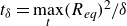 $t_{\delta } = \max \limits _t(R_{\textit{eq}})^2 / \delta$
, where
$t_{\delta } = \max \limits _t(R_{\textit{eq}})^2 / \delta$
, where $\delta$
denotes thermal diffusivity for liquid water (
$\delta$
denotes thermal diffusivity for liquid water ( $\approx 10^{-7} \rm m^2\,s^{-1}$
) and for water vapour (
$\approx 10^{-7} \rm m^2\,s^{-1}$
) and for water vapour ( $\approx 2\times 10^{-5}\,\rm m^2\,s^{-1}$
). For a maximum bubble radius
$\approx 2\times 10^{-5}\,\rm m^2\,s^{-1}$
). For a maximum bubble radius $\max \limits _t(R_{\textit{eq}})$
of around 3 mm,
$\max \limits _t(R_{\textit{eq}})$
of around 3 mm, $t_{\delta } \approx 100\rm\, s$
in the liquid water and
$t_{\delta } \approx 100\rm\, s$
in the liquid water and $0.5\,\rm s$
inside the bubble. This significant time scale difference between bubble growth and advection transport time, and thermal diffusion in both liquid water and water vapour indicates that the water vapour inside the bubble is effectively thermally isolated for
$0.5\,\rm s$
inside the bubble. This significant time scale difference between bubble growth and advection transport time, and thermal diffusion in both liquid water and water vapour indicates that the water vapour inside the bubble is effectively thermally isolated for $R_{\textit{eq}} \gtrsim 3\,\rm mm$
with a gas velocity
$R_{\textit{eq}} \gtrsim 3\,\rm mm$
with a gas velocity $\lesssim 30\,\rm m\,s^{-1}$
. The volume of the bubble increases as the bubble expands, resulting in a drop in temperature due to the conservation of energy in the absence of significant heat exchange. Despite the presence of localised undercooled regions, the average temperature inside the bubble remains above the reference temperature of the surrounding liquid due to the persistence of high-temperature zones (see figures 23
c–25
c).
$\lesssim 30\,\rm m\,s^{-1}$
. The volume of the bubble increases as the bubble expands, resulting in a drop in temperature due to the conservation of energy in the absence of significant heat exchange. Despite the presence of localised undercooled regions, the average temperature inside the bubble remains above the reference temperature of the surrounding liquid due to the persistence of high-temperature zones (see figures 23
c–25
c).
Notably, the hottest region remains much closer to the wall than the bubble centroid throughout the entire bubble lifetime for the three regimes. In the early phase following bubble generation, the rapid expansion leads to a strong transient for the velocity field. This results in the advection of high-temperature fluid towards the wall, while the bubble centroid moves slightly away from the wall, particularly for smallest $\gamma$
, due to the fact that the bubble grows less on the near-wall interface than on the far-wall interface because of the presence of the wall causing asymmetric expansion that displaces the centroid away from the wall.
$\gamma$
, due to the fact that the bubble grows less on the near-wall interface than on the far-wall interface because of the presence of the wall causing asymmetric expansion that displaces the centroid away from the wall.
As the bubble continues to grow, the temperature location reaches a plateau in all cases (see, for example, the earliest 150 $\,\unicode{x03BC}\textrm{s}$
for
$\,\unicode{x03BC}\textrm{s}$
for $\gamma = 0.97$
in figure 23
d), indicating that the early advection driven by strong velocity gradients has subsided. A second and slower convective time scale then becomes apparent, associated with the transport of heat through bulk flow rather than sharp gradients. This results in a slower, nearly linear decline of the maximum temperature position toward the wall, even as the bubble centroid continues to migrate away. As
$\gamma = 0.97$
in figure 23
d), indicating that the early advection driven by strong velocity gradients has subsided. A second and slower convective time scale then becomes apparent, associated with the transport of heat through bulk flow rather than sharp gradients. This results in a slower, nearly linear decline of the maximum temperature position toward the wall, even as the bubble centroid continues to migrate away. As $\gamma$
increases to 1.64, the influence of the wall becomes less dominant. The bubble exhibits a more symmetric expansion and there is a negligible shift of the bubble centroid away from the wall (as shown in figure 25
d). The maximum temperature location remains closer to the wall than the bubble centroid, but its decline is more gradual, reflecting the weaker wall influence. In the case of
$\gamma$
increases to 1.64, the influence of the wall becomes less dominant. The bubble exhibits a more symmetric expansion and there is a negligible shift of the bubble centroid away from the wall (as shown in figure 25
d). The maximum temperature location remains closer to the wall than the bubble centroid, but its decline is more gradual, reflecting the weaker wall influence. In the case of $\gamma$
= 2.14, the wall effect becomes minimal, leading to the most symmetric bubble growth dynamics among the three cases. While the hottest region still stays closer to the wall than the bubble centroid, its position is the most stable and least offset, reflecting the minimal influence of the wall at larger stand-off ratios.
$\gamma$
= 2.14, the wall effect becomes minimal, leading to the most symmetric bubble growth dynamics among the three cases. While the hottest region still stays closer to the wall than the bubble centroid, its position is the most stable and least offset, reflecting the minimal influence of the wall at larger stand-off ratios.
Figures 23(e)–25(e) further illustrate the temporal evolution of the radial position of the maximum temperature point with respect to the z axis. During the initial expansion phase, the hottest region remains aligned with the zaxis due to the nearly spherical bubble shape. However, as the bubble begins to shrink and approaches the wall, axial cooling dissipates heat more effectively along the z axis, displacing the maximum temperature location away from the zaxis. During collapse, the bubble becomes highly compressed, and the maximum temperature region shifts back to the zaxis, exhibiting a more uniform distribution. More details of bubble dynamics at $t_c$
are reported in Appendix B. In the subsequent rebound phase, the bubble re-expands preferentially along the wall, further influencing the redistribution of heat inside the bubble.
$t_c$
are reported in Appendix B. In the subsequent rebound phase, the bubble re-expands preferentially along the wall, further influencing the redistribution of heat inside the bubble.
4.4. Thermodynamics inside the bubble
The interplay between thermodynamic quantities is crucial for understanding the physical mechanism behind the cavitation bubble growth and collapse, especially as the temperature can reach several thousands of Kelvin as the gas (Dular & Coutier-Delgosha Reference Dular and Coutier-Delgosha2013; Bidi Reference Bidi2023). To gain deeper insight into this mechanism, in this section we investigate the dynamics of density, pressure and temperature inside the bubble as a function of $\gamma$
, which varies from 0.79 to 2.14. First of all, we present the temporal evolution of the maximum and mean value of each quantity at different
$\gamma$
, which varies from 0.79 to 2.14. First of all, we present the temporal evolution of the maximum and mean value of each quantity at different $\gamma$
. Then we analyse the relationship between the average internal thermodynamic quantities and
$\gamma$
. Then we analyse the relationship between the average internal thermodynamic quantities and $\gamma$
. All the simulations are carried out using the absorption coefficient reported in table 2.
$\gamma$
. All the simulations are carried out using the absorption coefficient reported in table 2.
Temporal evolution of maximum and average temperature (a), density (b) and pressure (c) at different $\gamma$
inside the bubble.
$\gamma$
inside the bubble.

Figure 26 shows the temporal evolution of the maximum and average thermodynamic quantities as a function of $\gamma$
. The results indicate that the thermodynamic properties inside the bubble are significantly influenced by
$\gamma$
. The results indicate that the thermodynamic properties inside the bubble are significantly influenced by $\gamma$
, with all three quantities following a similar temporal trend. Specifically, they exhibit an increasing trend during the bubble collapse, reaching a spike at
$\gamma$
, with all three quantities following a similar temporal trend. Specifically, they exhibit an increasing trend during the bubble collapse, reaching a spike at $t\approx t_c$
followed by a subsequent decrease during the bubble rebound phase. This behaviour can be explained by the EoS. As
$t\approx t_c$
followed by a subsequent decrease during the bubble rebound phase. This behaviour can be explained by the EoS. As $\gamma$
increases, the average gas pressure, temperature and density also increase during the first collapse phase, as shown in figure 27. This is expected, considering that spherical collapses (
$\gamma$
increases, the average gas pressure, temperature and density also increase during the first collapse phase, as shown in figure 27. This is expected, considering that spherical collapses ( $\gamma \rightarrow \infty$
) are the most energetic with the stronger pressure wave releases. In particular, figure 26(a) shows the evolution of maximum and average internal temperatures over time for different
$\gamma \rightarrow \infty$
) are the most energetic with the stronger pressure wave releases. In particular, figure 26(a) shows the evolution of maximum and average internal temperatures over time for different $\gamma$
. During the bubble collapse phase, the internal temperature ranges from approximately 600 K to 3700 K. Additionally, as
$\gamma$
. During the bubble collapse phase, the internal temperature ranges from approximately 600 K to 3700 K. Additionally, as $\gamma$
increases, the peak temperature occurs earlier as
$\gamma$
increases, the peak temperature occurs earlier as $t_c$
is shorter. Specifically, as
$t_c$
is shorter. Specifically, as $\gamma$
increases from 0.79 to 2.14, the time at which the peak temperature is reached (
$\gamma$
increases from 0.79 to 2.14, the time at which the peak temperature is reached ( $t_{{\textit{max}}(T_{\textit{avg}})}$
) decreases from 633.20
$t_{{\textit{max}}(T_{\textit{avg}})}$
) decreases from 633.20 $\mu$
s to 565.10
$\mu$
s to 565.10 $\mu$
s as
$\mu$
s as $t_c$
is shorter.
$t_c$
is shorter.
Relationship among the average internal pressure, temperature and density with $\gamma$
during the first collapse phase.
$\gamma$
during the first collapse phase.

Comparison of collapse time $t_c$
and the timing of maximum average internal pressure
$t_c$
and the timing of maximum average internal pressure $t_{{\textit{max}}(P_{\textit{avg}})}$
, density
$t_{{\textit{max}}(P_{\textit{avg}})}$
, density $t_{{\textit{max}}(\rho _{\textit{avg}})}$
and temperature
$t_{{\textit{max}}(\rho _{\textit{avg}})}$
and temperature $t_{{\textit{max}}(T_{\textit{avg}})}$
as functions of
$t_{{\textit{max}}(T_{\textit{avg}})}$
as functions of $\gamma$
.
$\gamma$
.

The differences among the collapse time $t_c$
, the times corresponding to maximum average internal pressure
$t_c$
, the times corresponding to maximum average internal pressure $t_{{\textit{max}}(P_{\textit{avg}})}$
, density
$t_{{\textit{max}}(P_{\textit{avg}})}$
, density $t_{{\textit{max}}(\rho _{\textit{avg}})}$
and temperature
$t_{{\textit{max}}(\rho _{\textit{avg}})}$
and temperature $t_{{\textit{max}}(T_{\textit{avg}})}$
are compared in figure 28. The results indicate that as
$t_{{\textit{max}}(T_{\textit{avg}})}$
are compared in figure 28. The results indicate that as $\gamma$
increases, all characteristic times systematically decrease. This suggests that the bubble closer to the wall experiences a delayed collapse, while that farther away collapses more rapidly. Furthermore, the nearly perfect agreement among these four critical times implies that the peak in the average internal pressure, density and temperature occur almost simultaneously with the collapse, highlighting the strong coupling of thermodynamic and hydrodynamic processes during bubble collapse. Given the minimal difference among these time instants, we simplify our analysis by using
$\gamma$
increases, all characteristic times systematically decrease. This suggests that the bubble closer to the wall experiences a delayed collapse, while that farther away collapses more rapidly. Furthermore, the nearly perfect agreement among these four critical times implies that the peak in the average internal pressure, density and temperature occur almost simultaneously with the collapse, highlighting the strong coupling of thermodynamic and hydrodynamic processes during bubble collapse. Given the minimal difference among these time instants, we simplify our analysis by using $t_c$
as the representative time for
$t_c$
as the representative time for $t_{{\textit{max}}(P_{\textit{avg}})}$
,
$t_{{\textit{max}}(P_{\textit{avg}})}$
, $t_{{\textit{max}}(\rho _{\textit{avg}})}$
and
$t_{{\textit{max}}(\rho _{\textit{avg}})}$
and $t_{{\textit{max}}(T_{\textit{avg}})}$
in the following discussion.
$t_{{\textit{max}}(T_{\textit{avg}})}$
in the following discussion.
In terms of the density and pressure, figures 26(b) and 26(c) show the maximum and average internal bubble pressure and density evolution over time for $\gamma$
from 0.79 to 2.14. Owing to compressibility, the bubble pressure and density increase during the collapse stage. The pressure and density change become extremely large when the bubble reaches its minimum radius at
$\gamma$
from 0.79 to 2.14. Owing to compressibility, the bubble pressure and density increase during the collapse stage. The pressure and density change become extremely large when the bubble reaches its minimum radius at $t_c$
. The peak bubble pressure and density are observed when
$t_c$
. The peak bubble pressure and density are observed when $\gamma$
is largest, i.e.
$\gamma$
is largest, i.e. $\gamma$
= 2.14, at the first bubble collapse stage, with a value of approximately 62 MPa and 45
$\gamma$
= 2.14, at the first bubble collapse stage, with a value of approximately 62 MPa and 45 $\rm kg\,m^{-3}$
. Subsequently, the bubble pressure and density decreased during the rebound stage.
$\rm kg\,m^{-3}$
. Subsequently, the bubble pressure and density decreased during the rebound stage.
Comparison of the numerical solution for $\gamma =1.31$
and NASG theoretical solution. (a) Temporal evolution of the average internal pressure. (b) Temporal evolution of the average internal density. (c) Temporal evolution of the average internal temperature. For each subfigure, the inset shows a zoomed-in section between 530–630
$\gamma =1.31$
and NASG theoretical solution. (a) Temporal evolution of the average internal pressure. (b) Temporal evolution of the average internal density. (c) Temporal evolution of the average internal temperature. For each subfigure, the inset shows a zoomed-in section between 530–630 $\,\unicode{x03BC}\textrm{s}$
.
$\,\unicode{x03BC}\textrm{s}$
.

Figure 29 shows a comparative analysis of one numerical case for $\gamma =1.31$
and the theoretical predictions based on the NASG EoS assuming equilibrium for the average thermodynamic fields inside the bubble. Here, the NASG EoS is used to reconstruct one thermodynamic quantity from the other two. At each time instant, two spatially averaged quantities, for instance, bubble temperature and density, are inserted into the NASG EoS to compute the third quantity, i.e. pressure.
$\gamma =1.31$
and the theoretical predictions based on the NASG EoS assuming equilibrium for the average thermodynamic fields inside the bubble. Here, the NASG EoS is used to reconstruct one thermodynamic quantity from the other two. At each time instant, two spatially averaged quantities, for instance, bubble temperature and density, are inserted into the NASG EoS to compute the third quantity, i.e. pressure.
A noticeable difference is observed in terms of the temporal evolution of temperature (figure 29
c) compared with pressure (figure 29
a) and density (figure 29
b). Temperature initially exhibits a non-negligible deviation, likely due to the fact that the liquid is preheated before bubble formation in laser-induced cavitation, creating a thermal memory effect that drives the initial evolution of the bubble significantly out-of-average equilibrium. After reaching its peak, temperature decreases more gradually, following a smooth transition rather than the rapid drops observed in pressure and density. This behaviour can be attributed to energy dissipation and heat retention, as well as the effects of thermal conductivity and heat diffusion. The internal energy, which governs temperature, dissipates progressively rather than sharply. Heat diffusion occurs at a slower rate quantified by $t_{\delta } = \min \limits _t(R_{\textit{eq}})^2 / \delta$
, where
$t_{\delta } = \min \limits _t(R_{\textit{eq}})^2 / \delta$
, where $\delta$
denotes thermal diffusivity, at around
$\delta$
denotes thermal diffusivity, at around $10^{-7}\rm\, m^2\,s^{-1}$
in the liquid water and
$10^{-7}\rm\, m^2\,s^{-1}$
in the liquid water and $2\times 10^{-5} \rm\,m^2\,s^{-1}$
in the gas. For a minimum bubble radius
$2\times 10^{-5} \rm\,m^2\,s^{-1}$
in the gas. For a minimum bubble radius $\min \limits _t(R_{\textit{eq}})$
of around 0.5 mm,
$\min \limits _t(R_{\textit{eq}})$
of around 0.5 mm, $t_{\delta }$
reaches approximately
$t_{\delta }$
reaches approximately $2.5\rm \,s$
in the liquid water and
$2.5\rm \,s$
in the liquid water and $1\rm\,s$
in the gas. Conversely, the rapid compression and rebound process is governed by the Rayleigh collapse time, which governs
$1\rm\,s$
in the gas. Conversely, the rapid compression and rebound process is governed by the Rayleigh collapse time, which governs $\ddot {R}$
, i.e.
$\ddot {R}$
, i.e. $t_R \approx 0.915 \min \limits _t(R_{\textit{eq}}) \sqrt {\rho /\Delta p} \approx 46 \,\unicode{x03BC}\textrm{s}$
, controlling the dynamics of pressure and density.
$t_R \approx 0.915 \min \limits _t(R_{\textit{eq}}) \sqrt {\rho /\Delta p} \approx 46 \,\unicode{x03BC}\textrm{s}$
, controlling the dynamics of pressure and density. $t_{\delta } \gg t_R$
leads to a more continuous and prolonged cooling phase.
$t_{\delta } \gg t_R$
leads to a more continuous and prolonged cooling phase.
Despite this deviation, the overall agreement across all thermodynamic variables demonstrates that spatial averaging provides a robust framework for linking non-equilibrium numerical simulations with average thermodynamic equilibrium predictions of the NASG EoS. This consistency validates that the averaged thermodynamic fields can reliably be modelled as in average thermodynamic equilibrium for most of the bubble lifetime, capturing the essential physics of bubble dynamics and cavitation phenomena near a wall.
5. Conclusion
In this work, a recent laser–fluid computational model was applied to study the physics behind a water vapour bubble induced by laser near a solid wall. The computational model combines laser energy absorption, vaporisation and thermodynamics of a compressible two-phase fluid flow, enabling the simulation of bubble formation, growth and collapse without predefining an initial bubble. The solver was employed for the first time for studying a wall-detached bubble. A broad range of stand-off ratios $\gamma \in [0.79,2.14]$
was investigated to assess the influence on the interfacial dynamics, collapse regimes and thermodynamics inside the bubble. Despite neglecting condensation, surface tension and viscous effects, the model reliably reproduces both qualitatively and quantitatively the experimental measurements for interfacial and wall pressure dynamics of a millimetric laser-induced bubble, provided that the right absorption coefficient is set to account for initial laser thermal energy absorption. To the best of the authors’ knowledge, this is the first time that such a detailed comparison is done on so many dynamical experimental measurements.
$\gamma \in [0.79,2.14]$
was investigated to assess the influence on the interfacial dynamics, collapse regimes and thermodynamics inside the bubble. Despite neglecting condensation, surface tension and viscous effects, the model reliably reproduces both qualitatively and quantitatively the experimental measurements for interfacial and wall pressure dynamics of a millimetric laser-induced bubble, provided that the right absorption coefficient is set to account for initial laser thermal energy absorption. To the best of the authors’ knowledge, this is the first time that such a detailed comparison is done on so many dynamical experimental measurements.
The comparison of interfacial dynamics between numerical simulations and experimental measurements demonstrates that the present model reliably reproduces the interfacial dynamics of laser-induced cavitation bubbles across a wide range of stand-off ratios. The simulated bubble shapes, collapse times and geometric evolution exhibit excellent agreement with experimental measurements, particularly during the expansion and early collapse stages. Minor discrepancies near the final collapse are attributed to sensitivity to the absorbed energy and experimental measurement uncertainties at small scales. The model accurately predicts the migration of the bubble centroid and the asymmetric interface motion leading to jet formation. Furthermore, the near-wall and far-wall interface velocities are captured with high fidelity, especially when the absorption coefficient is properly calibrated, confirming the model’s ability to resolve the strongly inertial jetting and rebound phenomena. These results validate the capability of the proposed two-phase compressible model to predict the complex interfacial dynamics of millimetric laser-induced bubbles near a wall.
Three distinct collapse regimes have been identified in the simulations, consistent with the experimental identification by Subramanian et al. (Reference Subramanian, Yang, Romanò and Coutier-Delgosha2026). The torus collapse regime occurs for $\gamma \leqslant 0.97$
, the mixed tip-and-torus collapse regime for
$\gamma \leqslant 0.97$
, the mixed tip-and-torus collapse regime for $1.13\leqslant \gamma \leqslant 1.46$
and the tip collapse regime for
$1.13\leqslant \gamma \leqslant 1.46$
and the tip collapse regime for $\gamma \geqslant 1.64$
. The wall pressure dynamics is found to be significantly affected by the initial energy absorbed by the gas phase solely in the mixed tip-and-torous collapse regime. This has been confirmed by additional simulations (not shown) for which we considered the pure-torous collapse and pure-tip collapse regimes for a range of absorption coefficients of 90 000
$\gamma \geqslant 1.64$
. The wall pressure dynamics is found to be significantly affected by the initial energy absorbed by the gas phase solely in the mixed tip-and-torous collapse regime. This has been confirmed by additional simulations (not shown) for which we considered the pure-torous collapse and pure-tip collapse regimes for a range of absorption coefficients of 90 000 $\rm\,m^{-1}$
to 110 000
$\rm\,m^{-1}$
to 110 000 $\rm\, m^{-1}$
without finding any major deviations to the reported results.
$\rm\, m^{-1}$
without finding any major deviations to the reported results.
After validating the robustness of the computational model against experimental results, the simulations reveal that increasing $\gamma$
leads to a more symmetric expansion, delayed jet impact and higher collapse pressures and temperatures. Conversely, smaller
$\gamma$
leads to a more symmetric expansion, delayed jet impact and higher collapse pressures and temperatures. Conversely, smaller $\gamma$
enhances the wall influence, resulting in asymmetric bubble expansion and early jet formation. Despite these quantitative differences, all cases share a rapid expansion, quasi-uniform bubble pressure at maximum volume, jet formation and violent collapse accompanied by strong pressure and temperature peaks. The simulations thus establish a coherent physical picture of how bubble–wall interaction controls the evolution of pressure, temperature and interface morphology across different collapse regimes.
$\gamma$
enhances the wall influence, resulting in asymmetric bubble expansion and early jet formation. Despite these quantitative differences, all cases share a rapid expansion, quasi-uniform bubble pressure at maximum volume, jet formation and violent collapse accompanied by strong pressure and temperature peaks. The simulations thus establish a coherent physical picture of how bubble–wall interaction controls the evolution of pressure, temperature and interface morphology across different collapse regimes.
The analysis of the thermodynamic evolution inside the bubble reveals a strong dependence on the stand-off ratio $\gamma$
. Both maximum and average values of pressure, density and temperature exhibit similar temporal behaviour, characterised by a sharp rise before collapse, a pronounced peak at
$\gamma$
. Both maximum and average values of pressure, density and temperature exhibit similar temporal behaviour, characterised by a sharp rise before collapse, a pronounced peak at $t \approx t_c$
and a rapid decay during rebound. Increasing
$t \approx t_c$
and a rapid decay during rebound. Increasing $\gamma$
leads to higher peak magnitudes and an earlier occurrence of these peaks, indicating that more spherical collapses produce stronger compression and heating effects. Comparison with the NASG EoS shows that spatially averaged pressure and density fields from the simulations follow equilibrium trends, even though the bubble dynamics is strongly non-equilibrium. The slower thermal relaxation relative to mechanical equilibrium highlights the persistence of out-of-average-equilibrium effects on the temperature, hence showing the importance of bubble temperature gradients after generation and after collapse. The bubble is far from an average thermodynamic equilibrium in its initial dynamics, especially for the temperature, which suggests that modelling approaches starting from a small bubble size and adjusted average pressure and density could lead to significant discrepancies in the evolution of a simulated bubble if the average temperature is set by enforcing the EoS. This is routinely done in the scientific literature and our study demonstrates that millimetric laser-induced bubbles are far from being realistically represented by such initial conditions. This has also been directly demonstrated comparing different initial conditions in our previous paper (Wang et al. Reference Wang, Yang and Romanò2026).
$\gamma$
leads to higher peak magnitudes and an earlier occurrence of these peaks, indicating that more spherical collapses produce stronger compression and heating effects. Comparison with the NASG EoS shows that spatially averaged pressure and density fields from the simulations follow equilibrium trends, even though the bubble dynamics is strongly non-equilibrium. The slower thermal relaxation relative to mechanical equilibrium highlights the persistence of out-of-average-equilibrium effects on the temperature, hence showing the importance of bubble temperature gradients after generation and after collapse. The bubble is far from an average thermodynamic equilibrium in its initial dynamics, especially for the temperature, which suggests that modelling approaches starting from a small bubble size and adjusted average pressure and density could lead to significant discrepancies in the evolution of a simulated bubble if the average temperature is set by enforcing the EoS. This is routinely done in the scientific literature and our study demonstrates that millimetric laser-induced bubbles are far from being realistically represented by such initial conditions. This has also been directly demonstrated comparing different initial conditions in our previous paper (Wang et al. Reference Wang, Yang and Romanò2026).
As a natural consequence of this conclusion, we point out that the most robust condition to model seems to be the bubble at its maximum volume, for which average thermodynamical quantities verify the equations of state. We however stress the need for modelling temperature and pressure gradients, as also pointed out in our previous study by Yang et al. (Reference Yang, Wang and Romanò2025).
Supplementary movies
Supplementary movies are available at https://doi.org/10.1017/jfm.2026.11781.
Funding
This work has been financially supported by the Chinese Scholarship Council (CSC) for B. Wang (student number 202206240030) and Z. Yang (student number 202008310185).
Declaration of interests
The authors report no conflict of interest.
Appendix A. Effect of EoS parameter values
We find that the behaviour of the bubble in the current laser–fluid computational framework can be affected by the choice of EoS. Here, we perform an additional simulation using a different set of EoS parameter values adopted from Métayer et al. (Reference Métayer, Saurel, Métayer and Saurel2016), while keeping all other physical and numerical parameters unchanged. Figure 30 compares the evolution of the equivalent bubble radius and wall pressure peak obtained from two different references of EoS parameter values for $\gamma =1.82$
. Overall, both simulations reproduce similar bubble dynamics over the entire cycle, with the bubble reaching its minimum size and wall pressure peak at the collapse time.
$\gamma =1.82$
. Overall, both simulations reproduce similar bubble dynamics over the entire cycle, with the bubble reaching its minimum size and wall pressure peak at the collapse time.
Comparison of simulation results obtained with different EoS parameter values for $\gamma = 1.82$
. (a) Evolution of the equivalent radius of the bubble. (b) Wall pressure peak.
$\gamma = 1.82$
. (a) Evolution of the equivalent radius of the bubble. (b) Wall pressure peak.

Nevertheless, some quantitative differences can be observed between the two cases.The maximum equivalent bubble radius obtained with the parameters of Zein et al. (Reference Zein, Hantke and Warnecke2013) is about 2.78 mm with collapse occurring at approximately 573 $\unicode{x03BC}\textrm{s}$
. In contrast, when using the parameters of Métayer et al. (Reference Métayer, Saurel, Métayer and Saurel2016), the maximum radius is slightly smaller, at 2.65 mm and the collapse occurs earlier at around 543
$\unicode{x03BC}\textrm{s}$
. In contrast, when using the parameters of Métayer et al. (Reference Métayer, Saurel, Métayer and Saurel2016), the maximum radius is slightly smaller, at 2.65 mm and the collapse occurs earlier at around 543 $\unicode{x03BC}\textrm{s}$
. Regarding the wall pressure, the simulation with Zein et al. (Reference Zein, Hantke and Warnecke2013) parameters yields pressure peaks of 12.5 MPa at collapse, and matches well with the experimental measurements by Subramanian et al. (Reference Subramanian, Yang, Romanò and Coutier-Delgosha2026), whereas the corresponding value with Métayer et al. (Reference Métayer, Saurel, Métayer and Saurel2016) parameters is 8.3MPa.
$\unicode{x03BC}\textrm{s}$
. Regarding the wall pressure, the simulation with Zein et al. (Reference Zein, Hantke and Warnecke2013) parameters yields pressure peaks of 12.5 MPa at collapse, and matches well with the experimental measurements by Subramanian et al. (Reference Subramanian, Yang, Romanò and Coutier-Delgosha2026), whereas the corresponding value with Métayer et al. (Reference Métayer, Saurel, Métayer and Saurel2016) parameters is 8.3MPa.
Appendix B. Temperature, density, pressure and velocity field inside the bubble at
$\boldsymbol{t}_{\boldsymbol{c}}$
for three cases

The axisymmetric simulation results for three different $\gamma$
, i.e.
$\gamma$
, i.e. $\gamma$
= 0.97. 1.64 and 2.14, presented in figure 31 together with figure 32, which shows the temperature, density, pressure and velocity distribution outside and inside the bubble, along with the liquid–gas interface depicted in a magenta colour at
$\gamma$
= 0.97. 1.64 and 2.14, presented in figure 31 together with figure 32, which shows the temperature, density, pressure and velocity distribution outside and inside the bubble, along with the liquid–gas interface depicted in a magenta colour at $t_c$
. Insets highlight the internal field of the bubble. Inside the bubble, the maximum temperature increases with
$t_c$
. Insets highlight the internal field of the bubble. Inside the bubble, the maximum temperature increases with $\gamma$
, reaching approximately 1793 K, 2833 K and 4226 K for
$\gamma$
, reaching approximately 1793 K, 2833 K and 4226 K for $\gamma$
= 0.97, 1.64 and 2.14, respectively. Similarly, the peak density rises from approximately 21
$\gamma$
= 0.97, 1.64 and 2.14, respectively. Similarly, the peak density rises from approximately 21 $\rm kg\,m^{-3}$
for
$\rm kg\,m^{-3}$
for $\gamma$
= 0.97 to 67
$\gamma$
= 0.97 to 67 $\rm kg\,m^{-3}$
for
$\rm kg\,m^{-3}$
for $\gamma$
= 2.14, highlighting stronger gas compression at larger distances from the wall. The internal pressure exhibits a significant increase, with maximum values of approximately 6.6 MPa, 23 MPa and 79 MPa, respectively. The velocity inside the bubble (see figure 32) also intensifies as
$\gamma$
= 2.14, highlighting stronger gas compression at larger distances from the wall. The internal pressure exhibits a significant increase, with maximum values of approximately 6.6 MPa, 23 MPa and 79 MPa, respectively. The velocity inside the bubble (see figure 32) also intensifies as $\gamma$
increases, with its magnitude rising from approximately 97 m s−1 for
$\gamma$
increases, with its magnitude rising from approximately 97 m s−1 for $\gamma$
= 0.97 to 240 m s−1 for
$\gamma$
= 0.97 to 240 m s−1 for $\gamma$
= 2.14. These trends suggest that at larger bubble centroid–wall distances, the internal thermodynamic extremes become more pronounced, leading to stronger compressive and convective effects within the bubble. Besides, the bubble collapse becomes more spherical as
$\gamma$
= 2.14. These trends suggest that at larger bubble centroid–wall distances, the internal thermodynamic extremes become more pronounced, leading to stronger compressive and convective effects within the bubble. Besides, the bubble collapse becomes more spherical as $\gamma$
increases. The velocity field depicted in figure 32 reveals that both flow intensities inside and outside the bubble increases with
$\gamma$
increases. The velocity field depicted in figure 32 reveals that both flow intensities inside and outside the bubble increases with $\gamma$
. The contraction speed of the bubble interface differs in the axial and radial directions, particularly for small
$\gamma$
. The contraction speed of the bubble interface differs in the axial and radial directions, particularly for small $\gamma$
, where the radial collapse is faster, causing the interface of the bubble to extend farther from the z axis, while the axial velocity becomes dominant as
$\gamma$
, where the radial collapse is faster, causing the interface of the bubble to extend farther from the z axis, while the axial velocity becomes dominant as $\gamma$
increases. This more axis-focused collapse trend is further supported by figure 33, which shows that both minimum and maximum quantities move closer to the z axis as
$\gamma$
increases. This more axis-focused collapse trend is further supported by figure 33, which shows that both minimum and maximum quantities move closer to the z axis as $\gamma$
increases, indicating that high intensity regions concentrate near the centreline.
$\gamma$
increases, indicating that high intensity regions concentrate near the centreline.
Temperature, density and pressure field (from top to bottom) at the collapse time for stand-off ratios (a) $\gamma$
= 0.97, (b)
$\gamma$
= 0.97, (b) $\gamma$
= 1.64, (c)
$\gamma$
= 1.64, (c) $\gamma$
= 2.14. The collapse time is denoted as
$\gamma$
= 2.14. The collapse time is denoted as $t_c$
and corresponds to
$t_c$
and corresponds to $t_c$
= 620.5
$t_c$
= 620.5 $\,\unicode{x03BC}\textrm{s}$
for
$\,\unicode{x03BC}\textrm{s}$
for $\gamma$
= 0.97,
$\gamma$
= 0.97, $t_c$
= 573
$t_c$
= 573 $\,\unicode{x03BC}\textrm{s}$
for
$\,\unicode{x03BC}\textrm{s}$
for $\gamma$
= 1.64,
$\gamma$
= 1.64, $t_c$
= 565.2
$t_c$
= 565.2 $\,\unicode{x03BC}\textrm{s}$
for
$\,\unicode{x03BC}\textrm{s}$
for $\gamma$
= 2.14. The wall is aligned with the left boundary in each subfigure. The inset images on the side magnify the bubble interior fields.
$\gamma$
= 2.14. The wall is aligned with the left boundary in each subfigure. The inset images on the side magnify the bubble interior fields.

Velocity field at the collapse time for stand-off ratios (a) $\gamma$
= 0.97, (b)
$\gamma$
= 0.97, (b) $\gamma$
= 1.64, (c)
$\gamma$
= 1.64, (c) $\gamma$
= 2.14. The collapse time is denoted as
$\gamma$
= 2.14. The collapse time is denoted as $t_c$
and corresponds to
$t_c$
and corresponds to $t_c$
= 620.5
$t_c$
= 620.5 $\,\unicode{x03BC}\textrm{s}$
for
$\,\unicode{x03BC}\textrm{s}$
for $\gamma$
= 0.97,
$\gamma$
= 0.97, $t_c$
= 573
$t_c$
= 573 $\,\unicode{x03BC}\textrm{s}$
for
$\,\unicode{x03BC}\textrm{s}$
for $\gamma$
= 1.64,
$\gamma$
= 1.64, $t_c$
= 565.2
$t_c$
= 565.2 $\,\unicode{x03BC}\textrm{s}$
for
$\,\unicode{x03BC}\textrm{s}$
for $\gamma$
= 2.14. The wall is aligned with the left boundary in each subfigure. The inset images on the side magnify the bubble interior fields.
$\gamma$
= 2.14. The wall is aligned with the left boundary in each subfigure. The inset images on the side magnify the bubble interior fields.

Radial position inside the bubble of peak values of the maximum and minimum pressure, temperature and density evolved over time as a function of $\gamma$
.
$\gamma$
.

Appendix C. Influence of the numerical boundary on the bubble shape
The potential reflection of shock waves at the numerical boundaries was carefully considered in the present simulations. To minimise boundary effects, the computational domain was chosen to be sufficiently large (55 times the maximum bubble size), and Neumann conditions were applied at the far-field boundary to ensure that outgoing waves do not reflect back. Moreover, upon an increase of the numerical domain, we do not observe any significant change in the bubble size during the early stage (tests done for $\gamma = 1.82$
; see figure 34). Regarding the effect of the solid wall, the bubble shape during the generation develops primarily along the laser beam direction. At this early time, e.g. at 78 ns, the bubble is sufficiently far from the wall compared with its current size, and the influence of the wall on the bubble shape during the generation process is negligible. The early bubble shape shows that the side closer to the laser plane is slightly wider than the opposite side at the nucleation point (see figure 35), which is consistent with experimental observations reported by Gonzalez-Avila et al. (Reference Gonzalez-Avila, Denner and Ohl2021).
$\gamma = 1.82$
; see figure 34). Regarding the effect of the solid wall, the bubble shape during the generation develops primarily along the laser beam direction. At this early time, e.g. at 78 ns, the bubble is sufficiently far from the wall compared with its current size, and the influence of the wall on the bubble shape during the generation process is negligible. The early bubble shape shows that the side closer to the laser plane is slightly wider than the opposite side at the nucleation point (see figure 35), which is consistent with experimental observations reported by Gonzalez-Avila et al. (Reference Gonzalez-Avila, Denner and Ohl2021).
Comparison of the bubble radius at the numerical domain size of 55 and 110 times the maximum bubble size.

(a) Experimental bubble shape and (b) computational bubble shape at 78 ns after the laser is on.

Case $\gamma = 1.64$
. The experimental top view of a cavitation bubble is indicated in black, while the orange mark presents the bubble shape calculated by our fitting algorithm. From left to right, the snapshots correspond to t = 65
$\gamma = 1.64$
. The experimental top view of a cavitation bubble is indicated in black, while the orange mark presents the bubble shape calculated by our fitting algorithm. From left to right, the snapshots correspond to t = 65 $\unicode{x03BC}\textrm{s}$
, 273
$\unicode{x03BC}\textrm{s}$
, 273 $\unicode{x03BC}\textrm{s}$
, 520
$\unicode{x03BC}\textrm{s}$
, 520 $\unicode{x03BC}\textrm{s}$
, 741
$\unicode{x03BC}\textrm{s}$
, 741 $\unicode{x03BC}\textrm{s}$
, respectively, while the collapse time is
$\unicode{x03BC}\textrm{s}$
, respectively, while the collapse time is $t_c = 572 \,\unicode{x03BC}\textrm{s}$
.
$t_c = 572 \,\unicode{x03BC}\textrm{s}$
.

Appendix D. Determination of equivalent bubble radius from the experimental visualisation
In the experiment, the equivalent radius of the bubble is measured from the top view using high-speed imaging, as shown in figure 36. There are generally five steps in our bubble characterisation protocol. (i) All relevant frames are extracted from the high-speed recordings. (ii) For each frame, the bubble interface coordinates $(r_b, z_b)$
are identified based on the index refraction contrast between liquid water and water vapour. (iii) The problem is simplified by assuming that the bubble growth is axisymmetric, allowing us to reflect part of the interfacial coordinates
$(r_b, z_b)$
are identified based on the index refraction contrast between liquid water and water vapour. (iii) The problem is simplified by assuming that the bubble growth is axisymmetric, allowing us to reflect part of the interfacial coordinates $(r_b, z_b)$
with respect to the axis. (iv) An in-house MATLAB code is then developed to fit the bubble interface using the fitting function
$(r_b, z_b)$
with respect to the axis. (iv) An in-house MATLAB code is then developed to fit the bubble interface using the fitting function $r_i^2 = a_0^2 - (z_i-a_1)^2\times (1+({a_2}/{z_i^{a_3}}))$
, where
$r_i^2 = a_0^2 - (z_i-a_1)^2\times (1+({a_2}/{z_i^{a_3}}))$
, where $a_0$
,
$a_0$
, $a_1$
,
$a_1$
, $a_2$
,
$a_2$
, $a_3$
are fitting parameters and
$a_3$
are fitting parameters and $z_i$
and
$z_i$
and $r_i$
denote axial and radial coordinates of the fitted interface. (v) The bubble volume is computed by revolving the fitted interface about the symmetry axis, and the equivalent bubble radius is finally obtained from the calculated volume assuming a spherical bubble of equal volume. For more details on the fitting function, we refer the reader to Yang et al. (Reference Yang, Wang and Romanò2025).
$r_i$
denote axial and radial coordinates of the fitted interface. (v) The bubble volume is computed by revolving the fitted interface about the symmetry axis, and the equivalent bubble radius is finally obtained from the calculated volume assuming a spherical bubble of equal volume. For more details on the fitting function, we refer the reader to Yang et al. (Reference Yang, Wang and Romanò2025).
This method provides accurate results during the expansion and early shrink phase (see figure 36 a–c), where the bubble shape remains relatively spherical and approximately axisymmetric. During the late collapse and rebound phases, however, the bubble interface becomes highly deformed and non-elliptic in the camera view due to the microjet penetration (see the experimental image reported in figure 36 d). Under these conditions, the fitting function can no longer guarantee reliable volume reconstruction, and the experiment equivalent radius after the late collapse and rebound phases are therefore not included in the numerical validation. In particular, as for a comparison after the first rebound, phase change is known to be significant starting from the first rebound phase (Yin et al. Reference Yin, Zhang, Zhu, Lv and Tian2021). Our physical model does not include phase transition beyond bubble generation, hence, the comparison between our simulations and the experiments is of limited use beyond the first collapse.
Appendix E. Sensitivity of the mixed tip-and-torus collapse regime to the initial condition
Figure 37(a) shows three independent experimental measurements conducted by Zhao & Coutier-Delgosha (Reference Zhao and Coutier-Delgosha2023), Yang et al. (Reference Yang, Wang and Romanò2025), Subramanian et al. (Reference Subramanian, Yang, Romanò and Coutier-Delgosha2026) within the same laboratory using the same apparatus. A significant statistical variance is observed in the mixed tip-and-torus collapse regime ( $1.13\leqslant \gamma \leqslant 1.46$
). In contrast, such variability is not observed in the purely torus (
$1.13\leqslant \gamma \leqslant 1.46$
). In contrast, such variability is not observed in the purely torus ( $\gamma \lt 1.13$
) and purely tip (
$\gamma \lt 1.13$
) and purely tip ( $\gamma \gt 1.46$
) collapse regimes. This discrepancy indicates that the mixed torus-and-tip regime is highly sensitive to initial conditions, making the repeatability of multiple experiments difficult to achieve even under controlled conditions. Consequently, attempting a strict quantitative prediction by simulation in this regime is inherently limited.
$\gamma \gt 1.46$
) collapse regimes. This discrepancy indicates that the mixed torus-and-tip regime is highly sensitive to initial conditions, making the repeatability of multiple experiments difficult to achieve even under controlled conditions. Consequently, attempting a strict quantitative prediction by simulation in this regime is inherently limited.
To further support this interpretation, we investigate the sensitivity of different collapse regimes to a change of the absorption coefficient, as shown in figure 37(b). The absorption coefficient $\alpha (I)$
increases and decreases slightly by 10
$\alpha (I)$
increases and decreases slightly by 10 $\%$
, respectively, for each
$\%$
, respectively, for each $\gamma$
, and the resulting changes in the maximum pressure at the wall centre are analysed. The results clearly show that the mixed regime shows a much stronger sensitivity to variation in the absorption coefficient
$\gamma$
, and the resulting changes in the maximum pressure at the wall centre are analysed. The results clearly show that the mixed regime shows a much stronger sensitivity to variation in the absorption coefficient $\alpha (I)$
compared with purely tip and purely torus collapse regimes. This confirms that the strong sensitivity is specific to the mixed regime and not observed in the two other collapse regimes.
$\alpha (I)$
compared with purely tip and purely torus collapse regimes. This confirms that the strong sensitivity is specific to the mixed regime and not observed in the two other collapse regimes.
(a) Comparison of the maximum wall pressure $\max \limits _t(p_w)$
among three experimental measurements by Zhao & Coutier-Delgosha (Reference Zhao and Coutier-Delgosha2023), Yang et al. (Reference Yang, Wang and Romanò2025), Subramanian et al. (Reference Subramanian, Yang, Romanò and Coutier-Delgosha2026), respectively, and the current numerical result. (b) Sensitivity of the maximum pressure at the wall centre to the absorption coefficient for all stand-off ratios
$\max \limits _t(p_w)$
among three experimental measurements by Zhao & Coutier-Delgosha (Reference Zhao and Coutier-Delgosha2023), Yang et al. (Reference Yang, Wang and Romanò2025), Subramanian et al. (Reference Subramanian, Yang, Romanò and Coutier-Delgosha2026), respectively, and the current numerical result. (b) Sensitivity of the maximum pressure at the wall centre to the absorption coefficient for all stand-off ratios $\gamma$
in the present study. The absorption coefficient is denoted by
$\gamma$
in the present study. The absorption coefficient is denoted by $\alpha (I)$
.
$\alpha (I)$
.

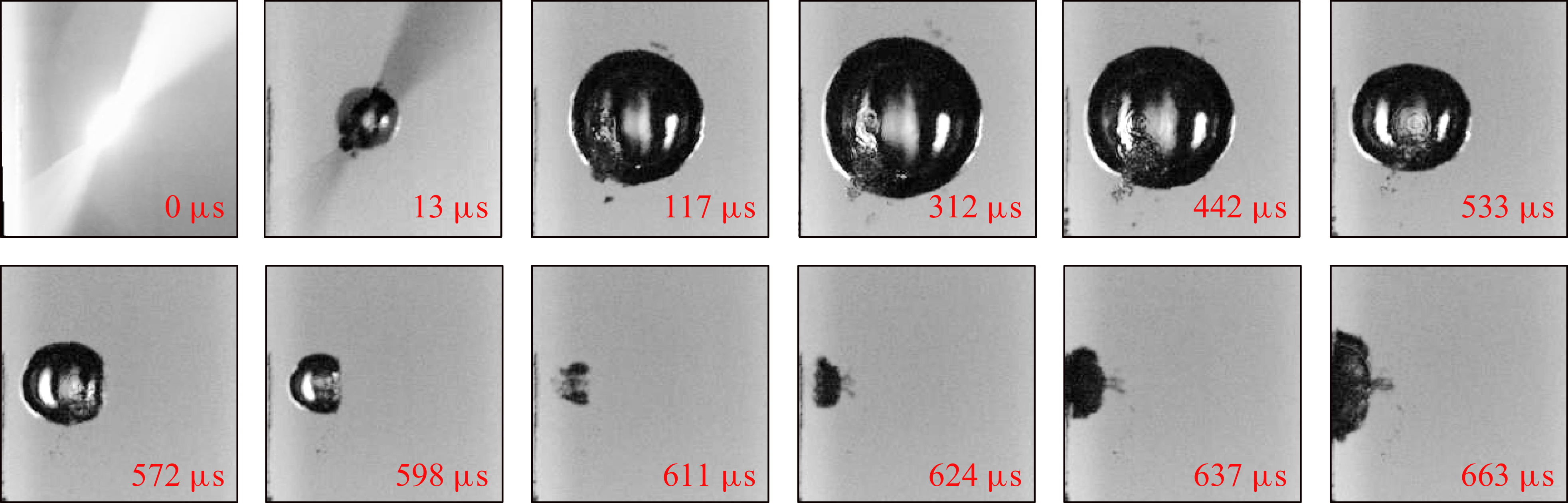
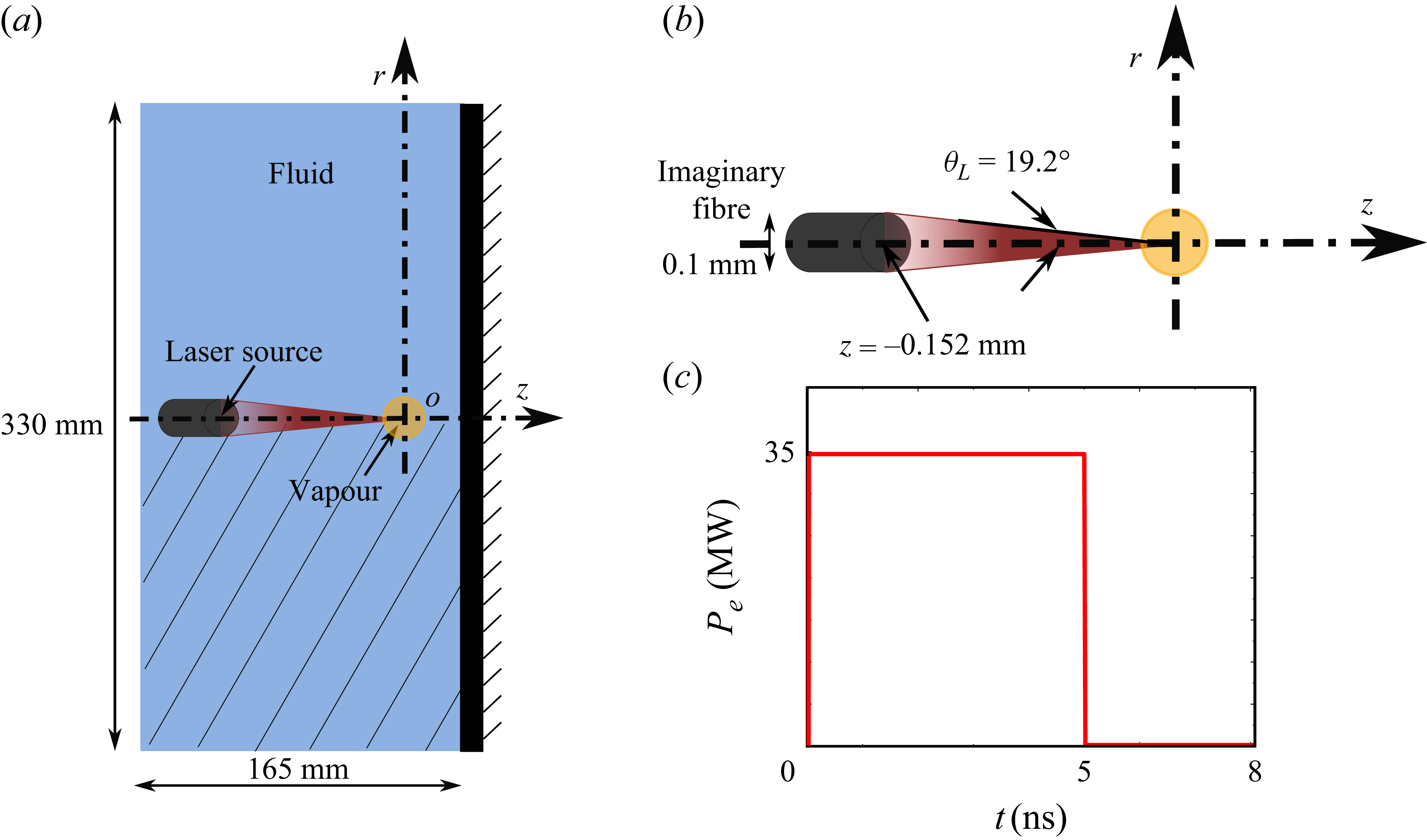
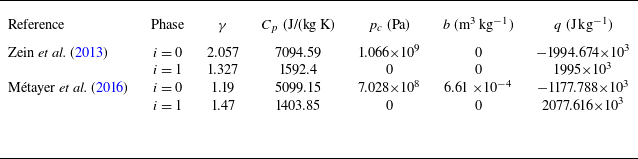
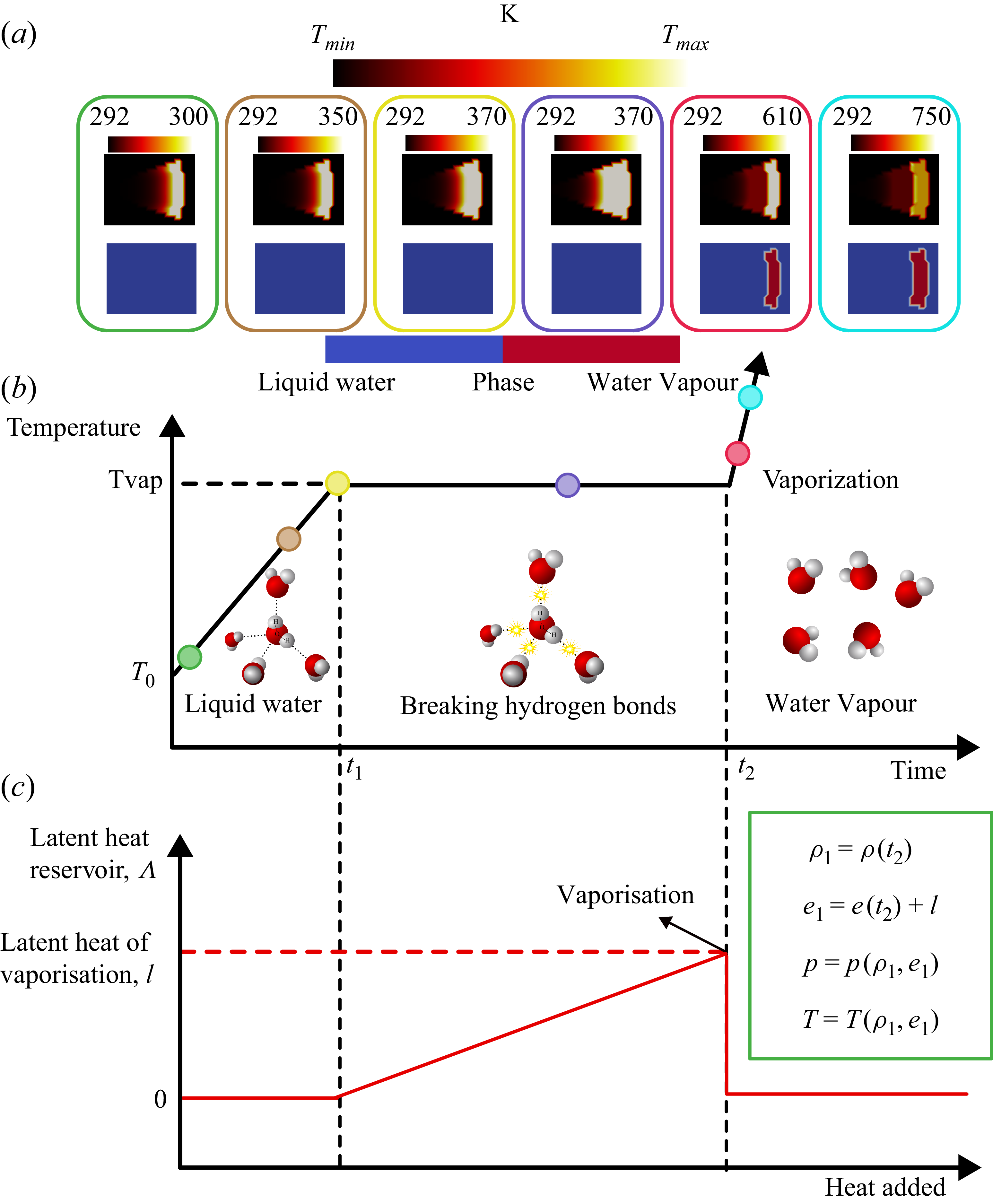
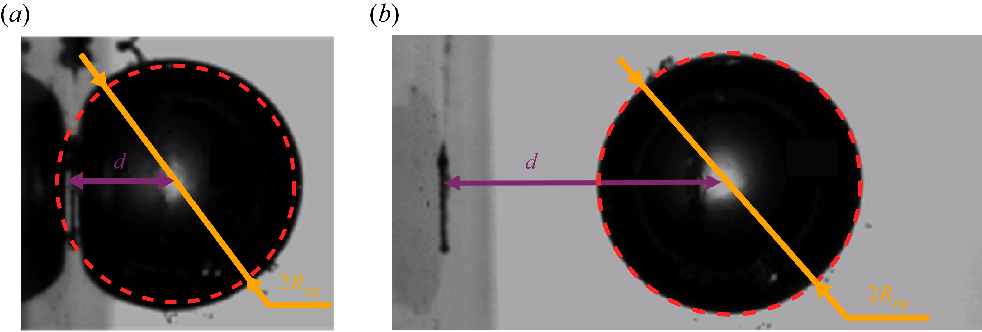
 γ
γ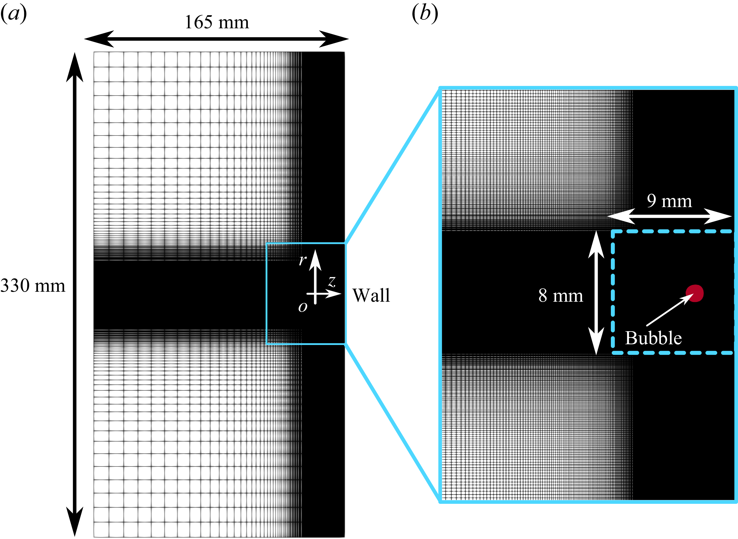
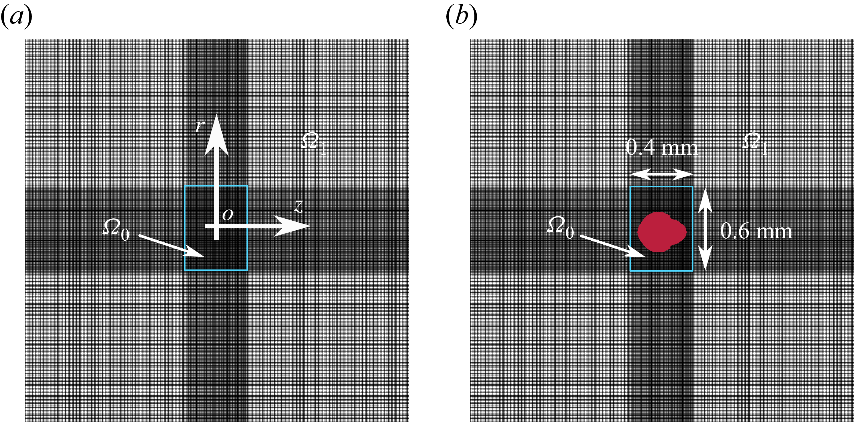
 t=0s
t=0s t=10−7s
 Ω0
Ω0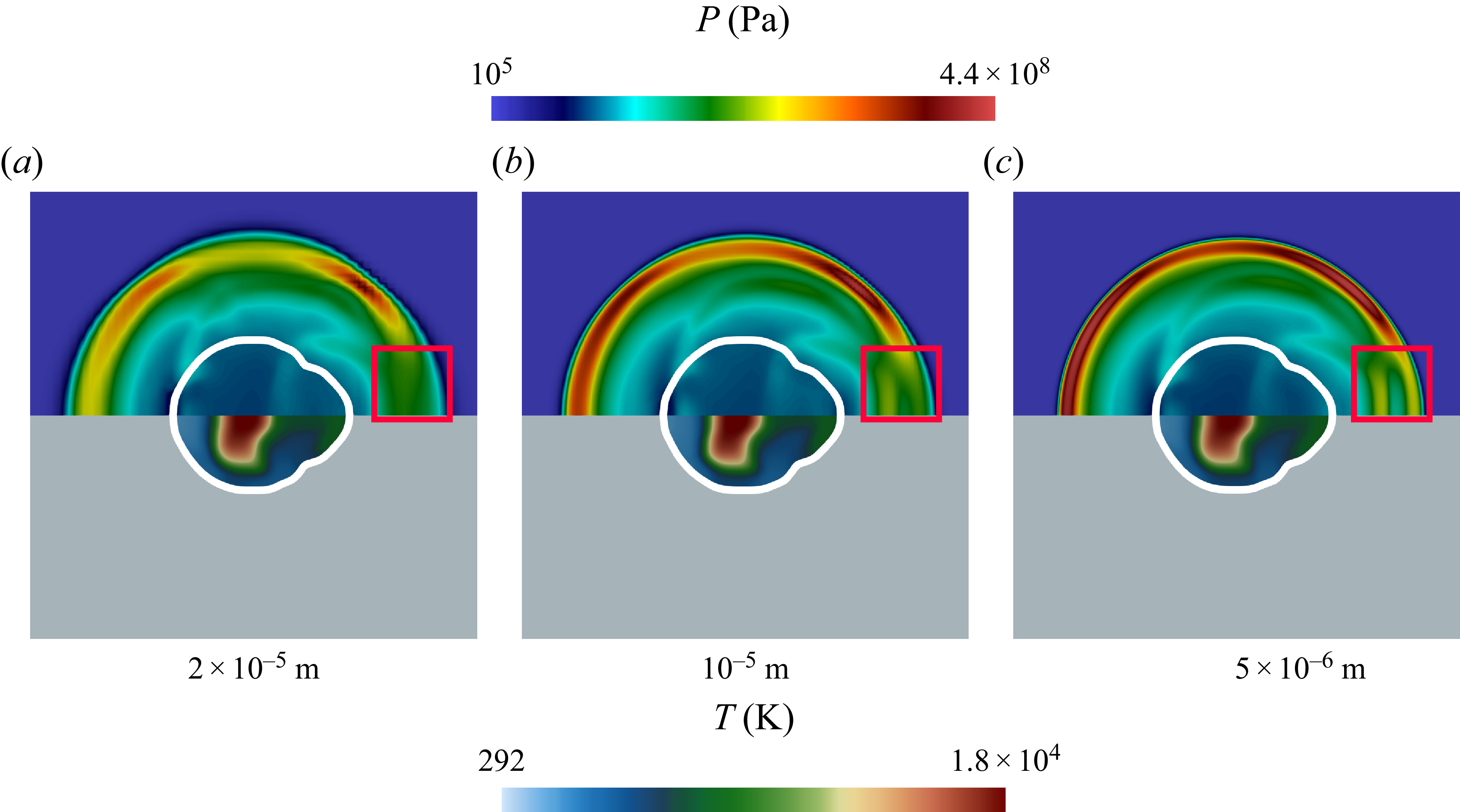
 t=2×10⁻⁷s
 Ω0
Ω0 Δx=5×10⁻⁶m
 Ω1
Ω1 Δx=2×10⁻⁵m
 5×10⁻⁶m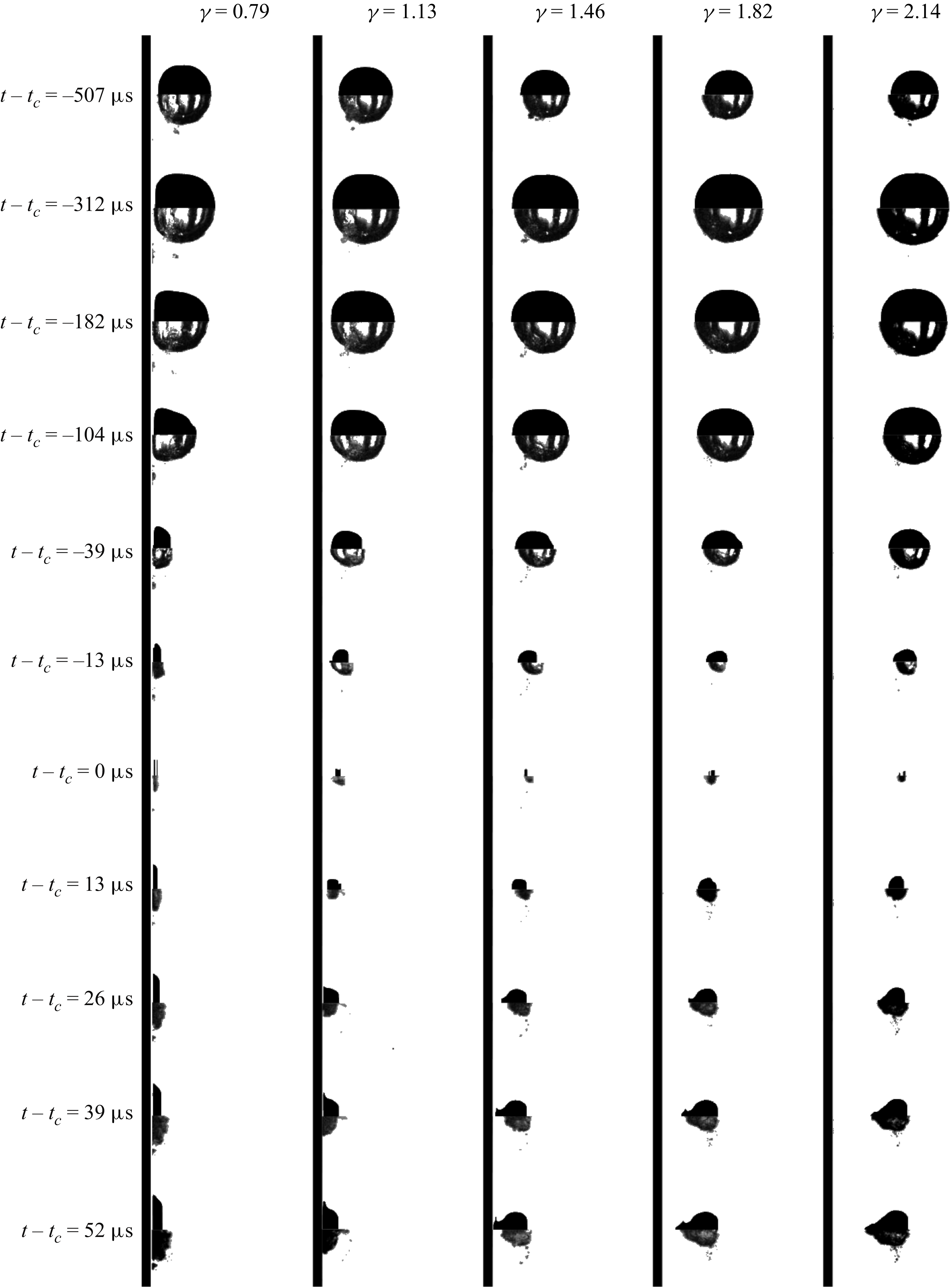
 tc
tc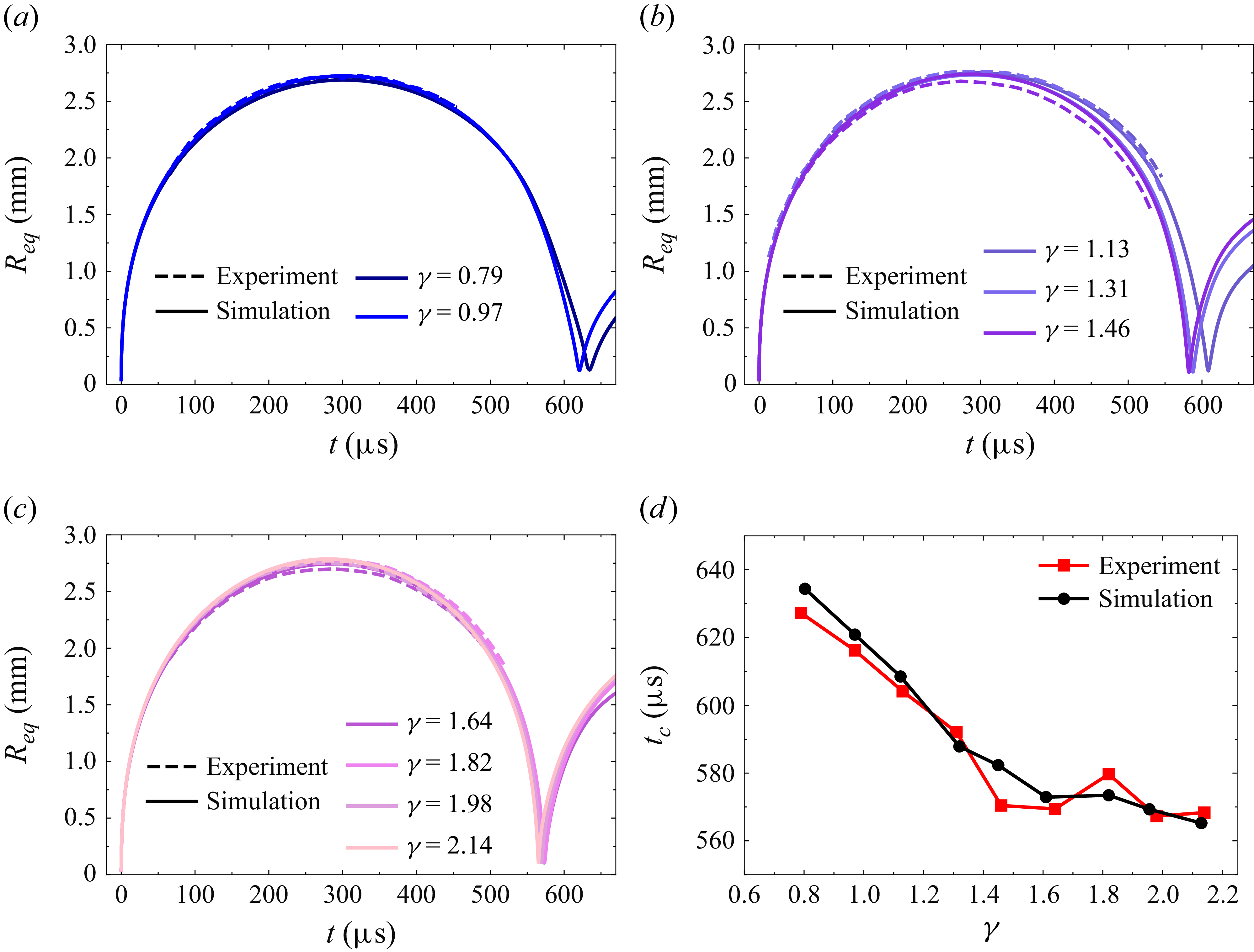
 γ
γ tc
tc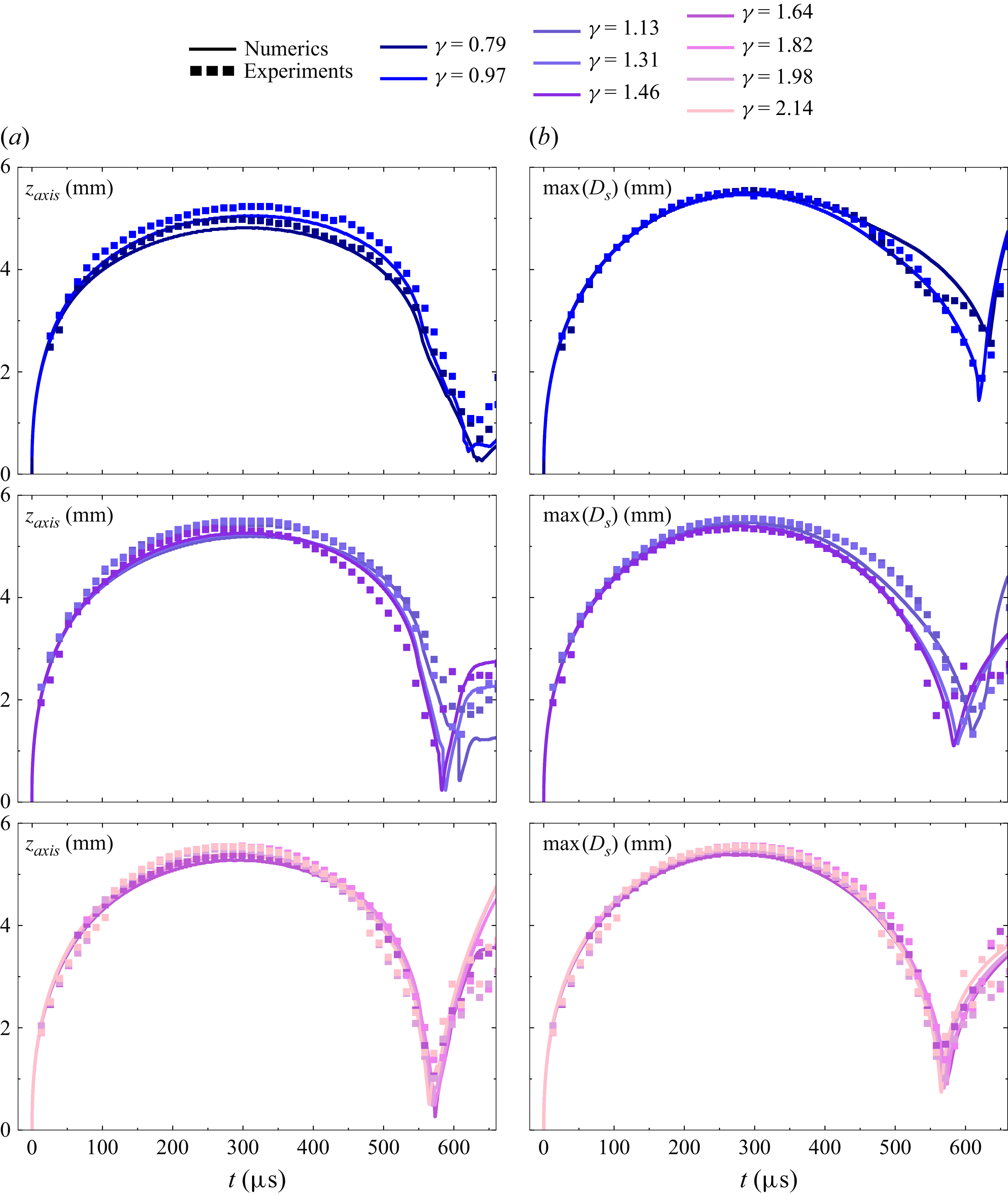
 zaxis
zaxis max(Ds)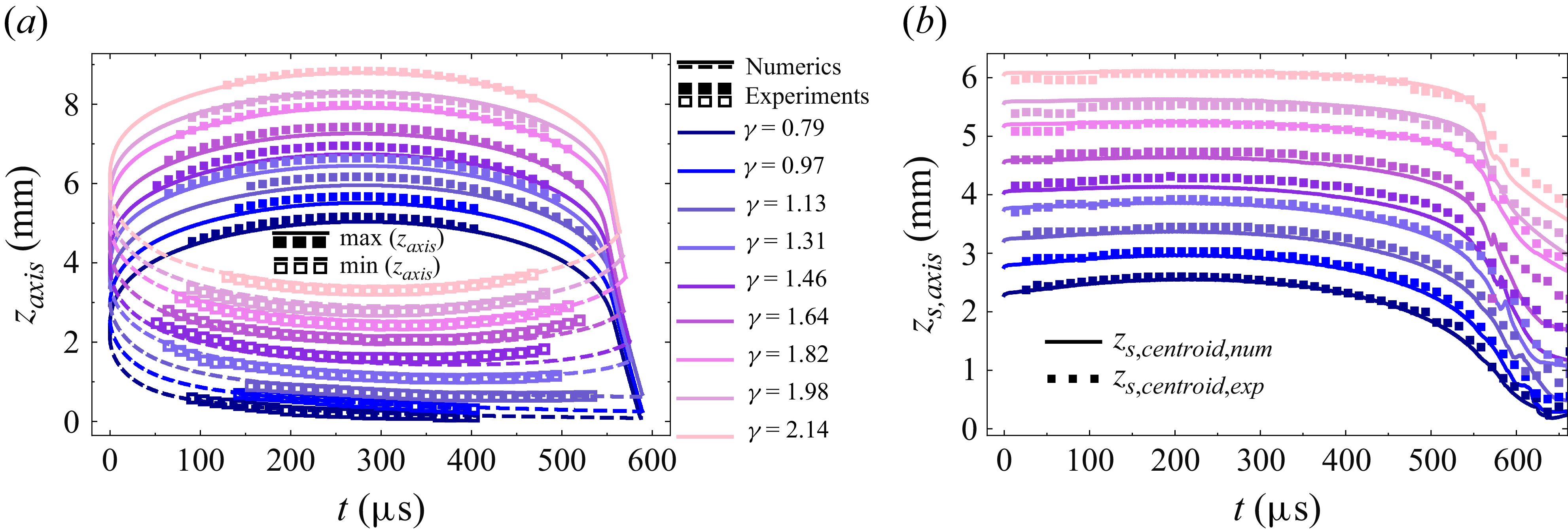
 z
z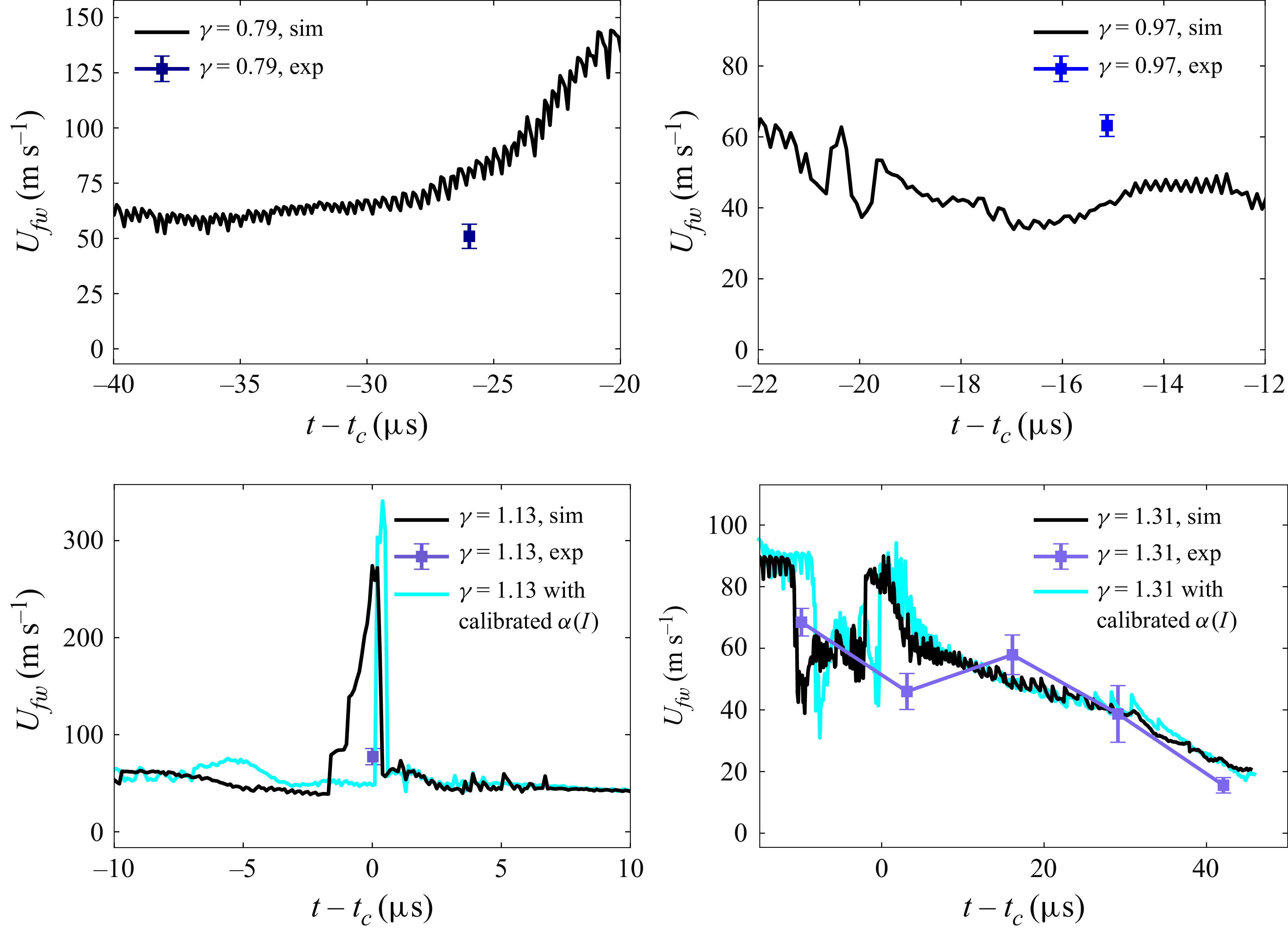
 Ufw
Ufw α(I)
α(I)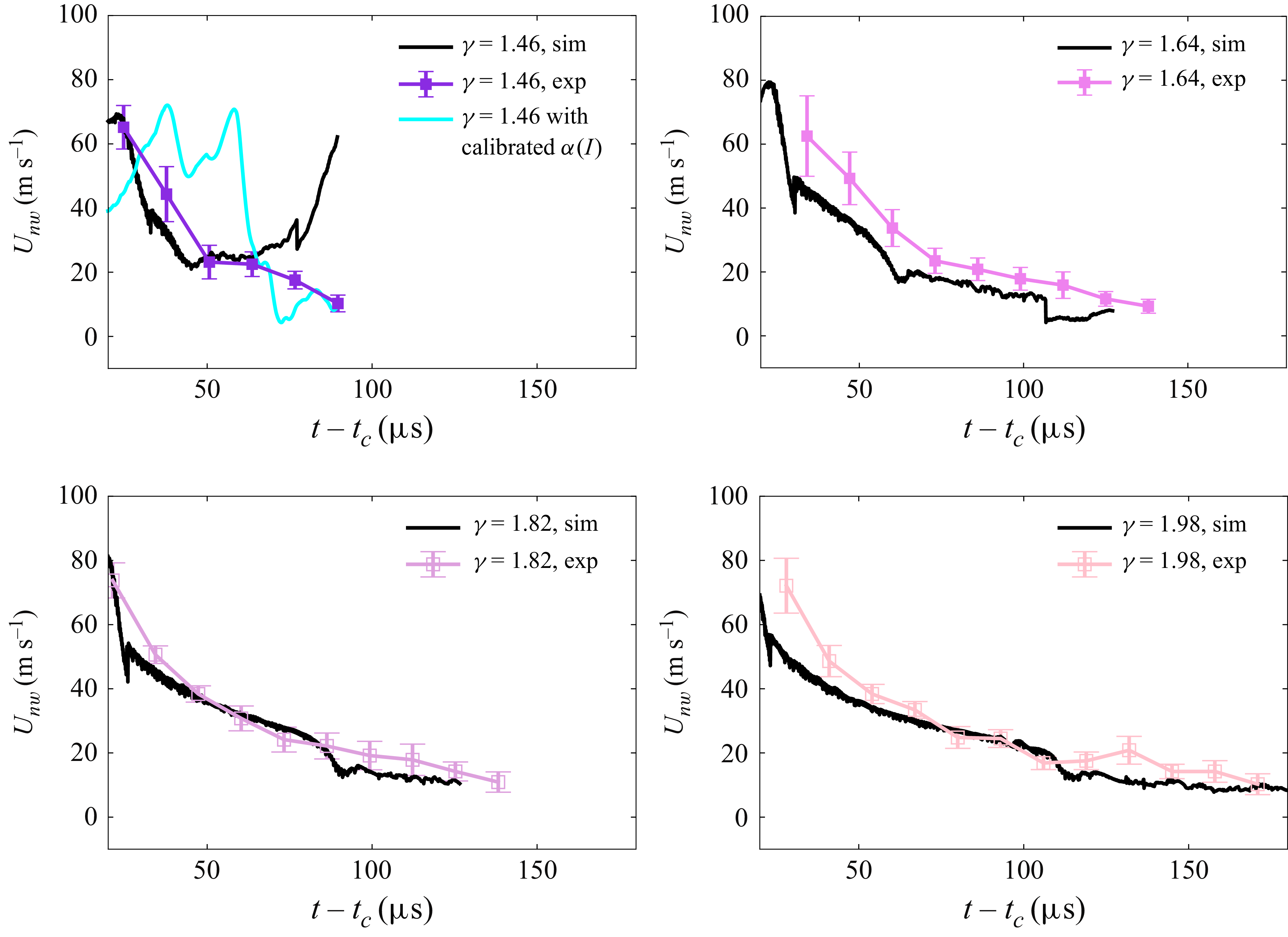
 Unw
Unw α(I)
α(I)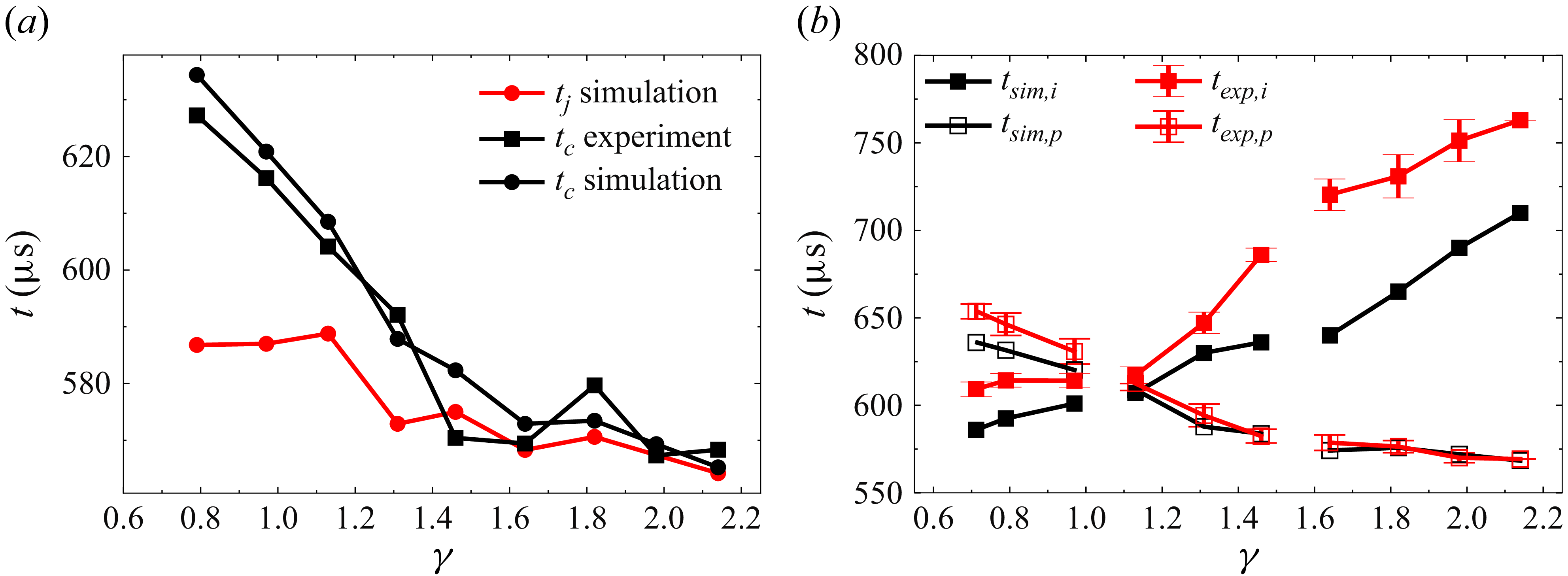
 tc
tc tj
tj tc
tc ti
ti tp
tp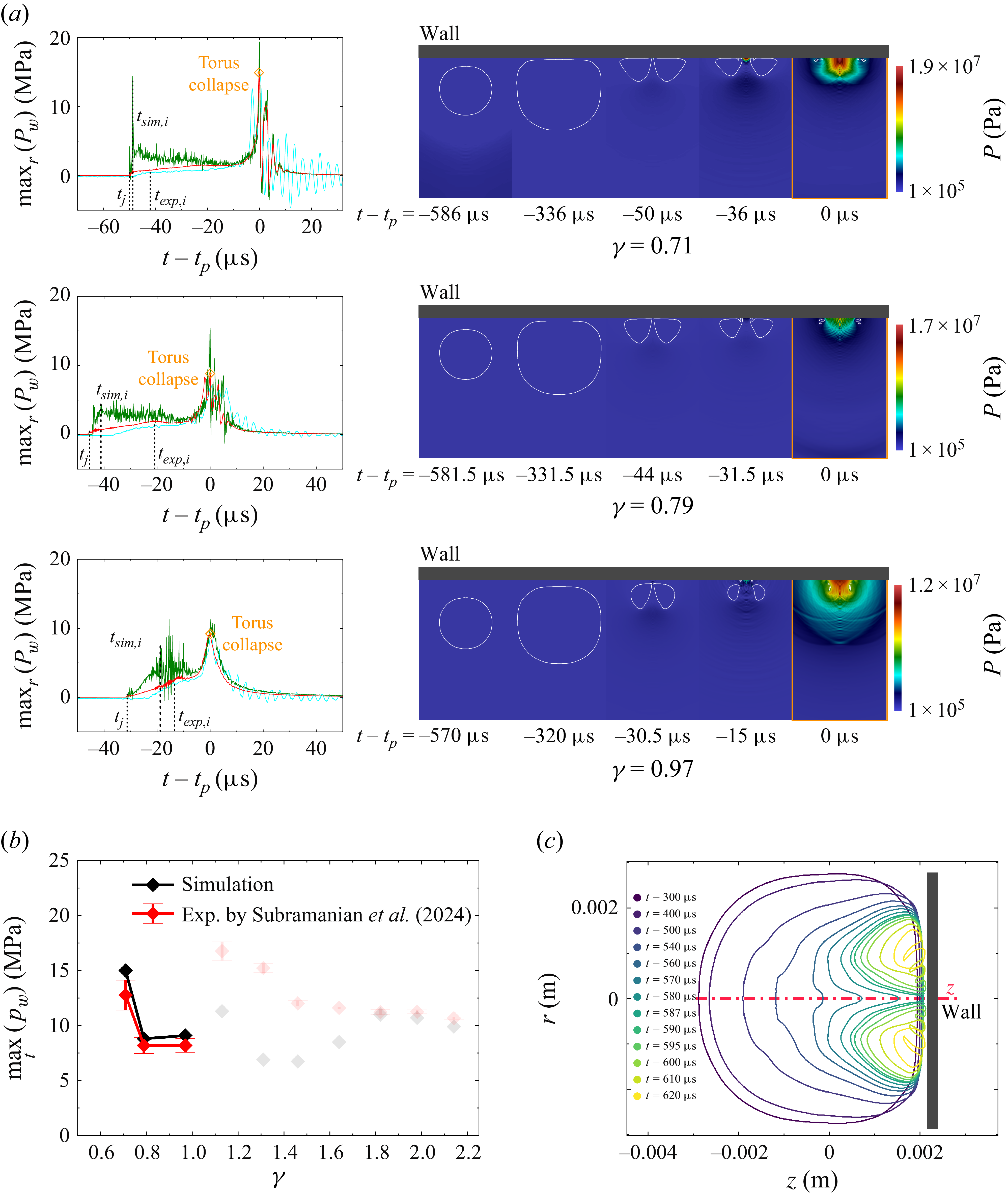
 γ∈[0.79,0.97]
 ti
ti tsim.,impact
 texp.,impact
 γ=0.79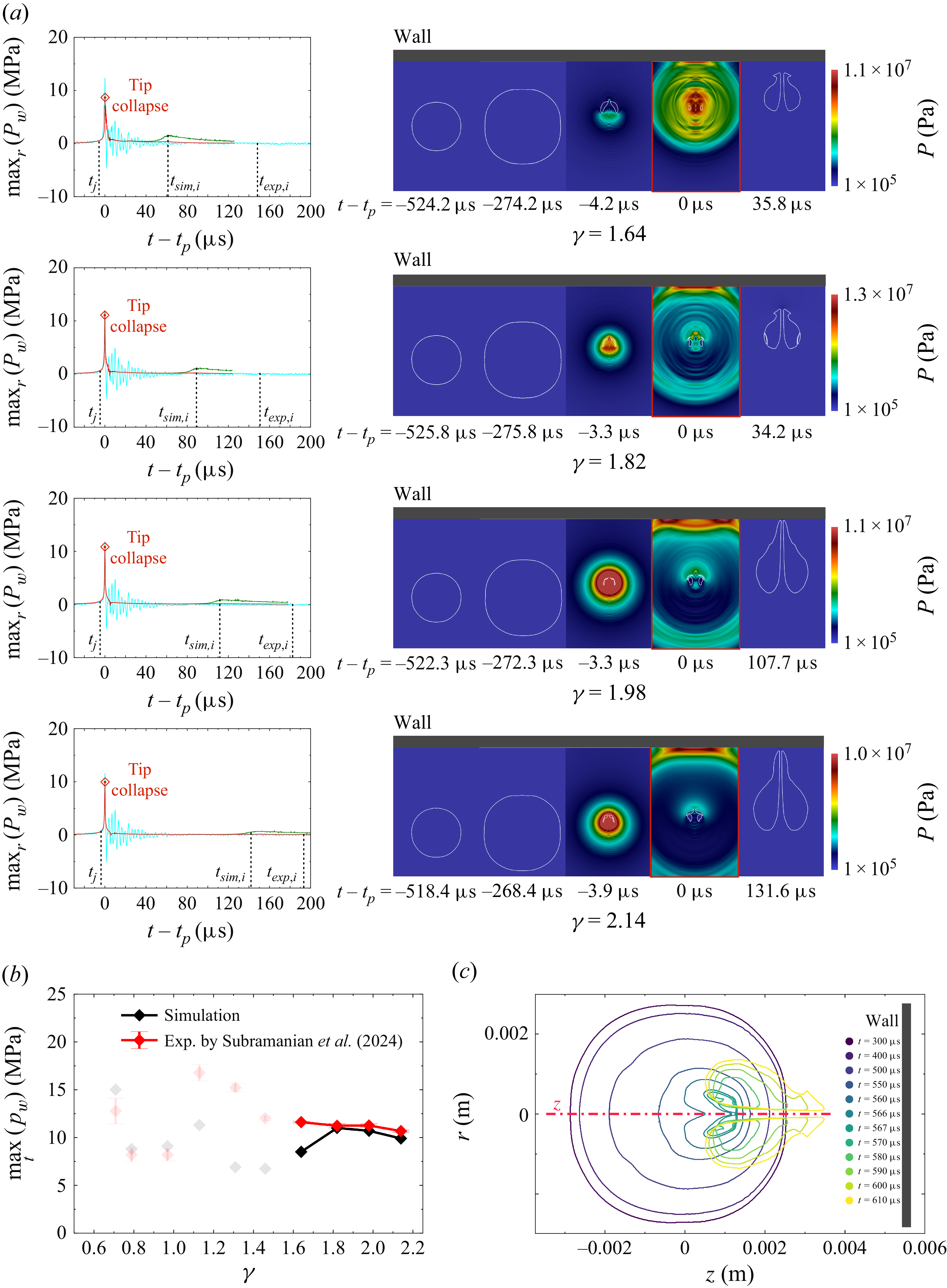
 γ∈[1.64,2.14]
 ti
ti tsim.,impact
 texp.,impact
 γ=1.98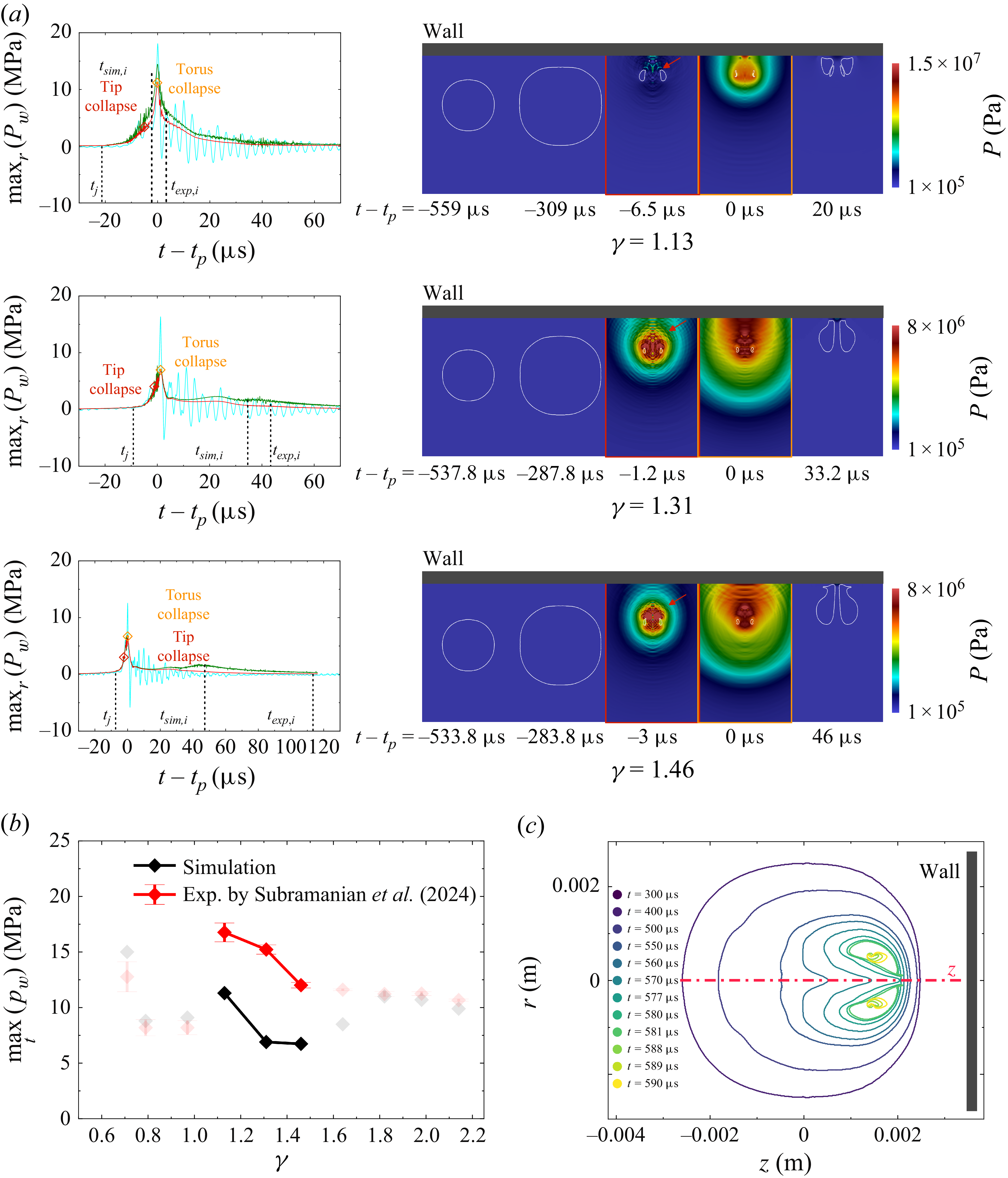
 γ∈[1.13,1.46]
 ti
ti tsim.,impact
 texp.,impact
 γ=1.31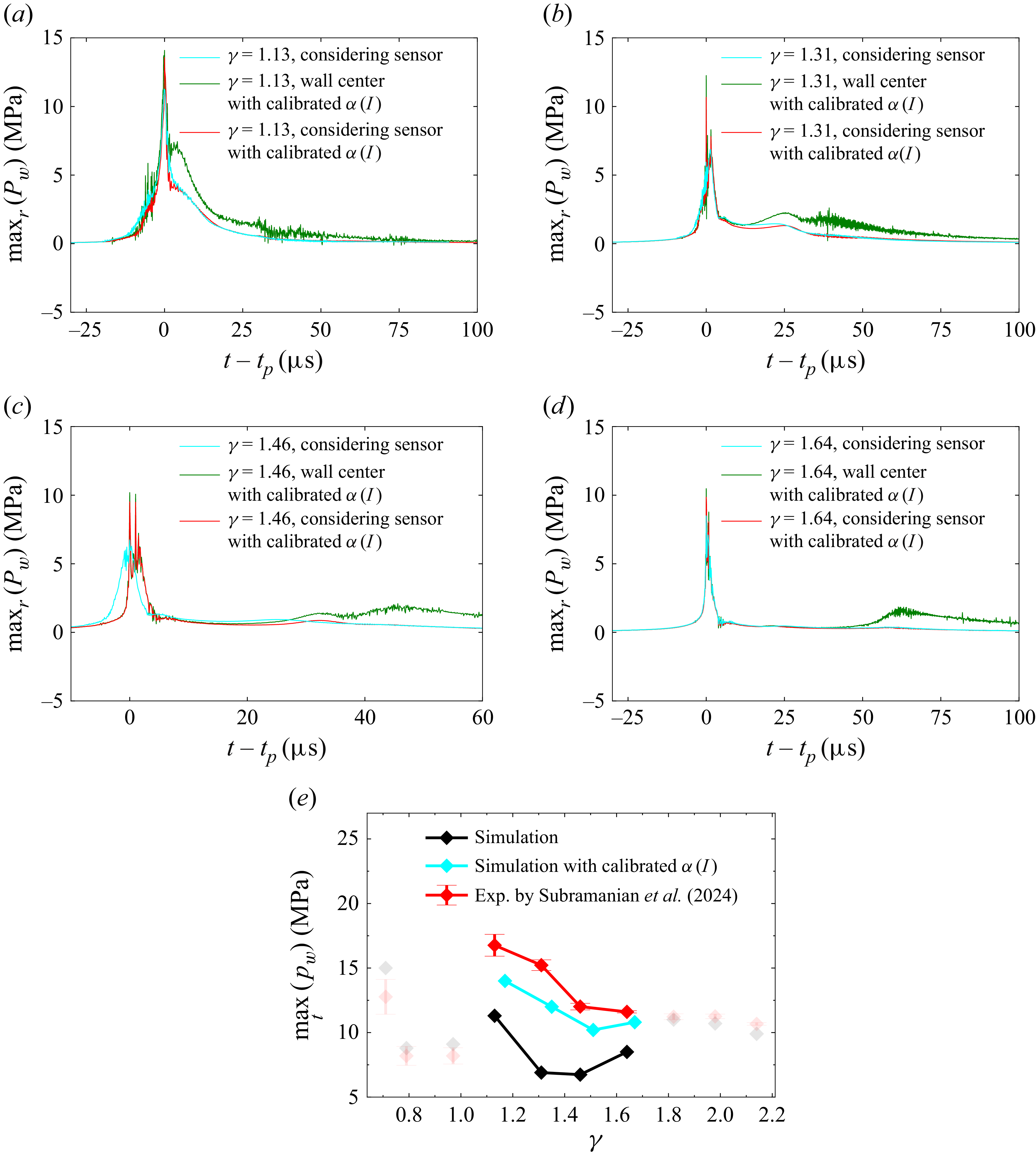
 γ
γ γ
γ γ
γ γ
γ α(I)
α(I)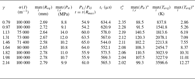
 γ
γ tc∗
tc∗ maxt,r(Pw)∗
 maxt(Tavg)∗
 maxt(Req)ρ0/Δp
 Δp
Δp T0
T0 Δp=PL−PG
 PL
PL PG
PG t=t(Rmax)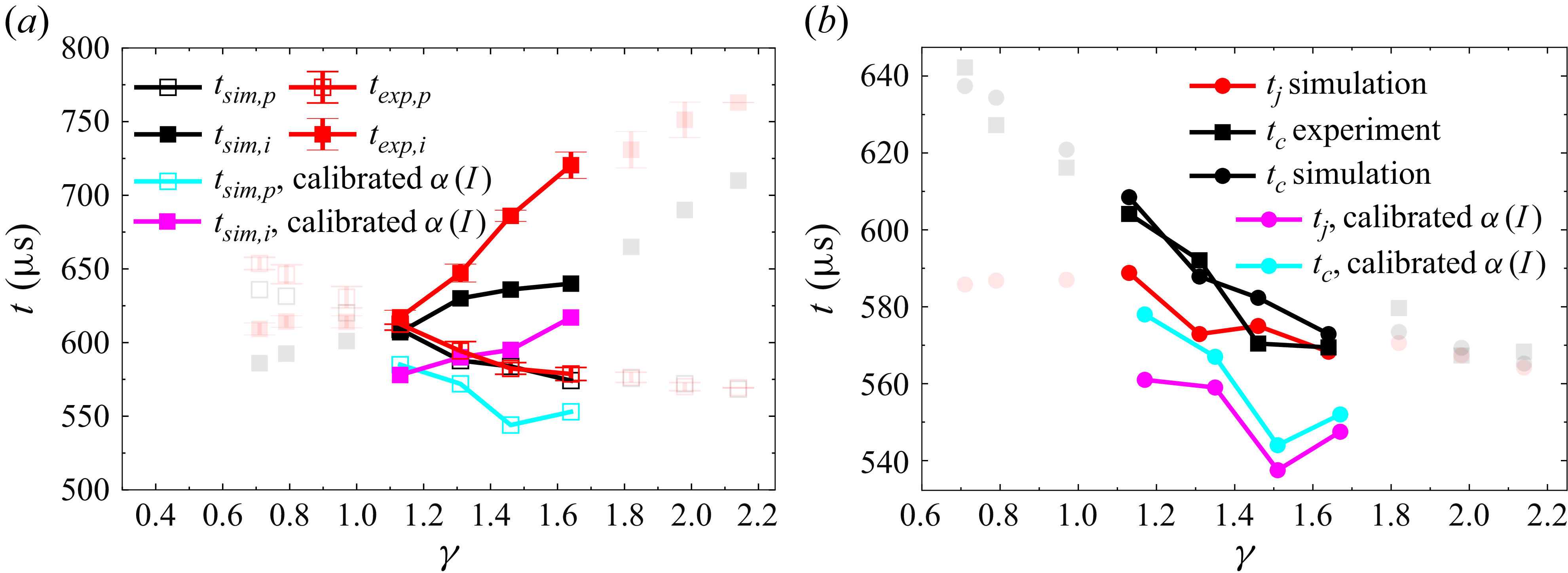
 ti
ti tc
tc tj
tj tc
tc α(I)
α(I)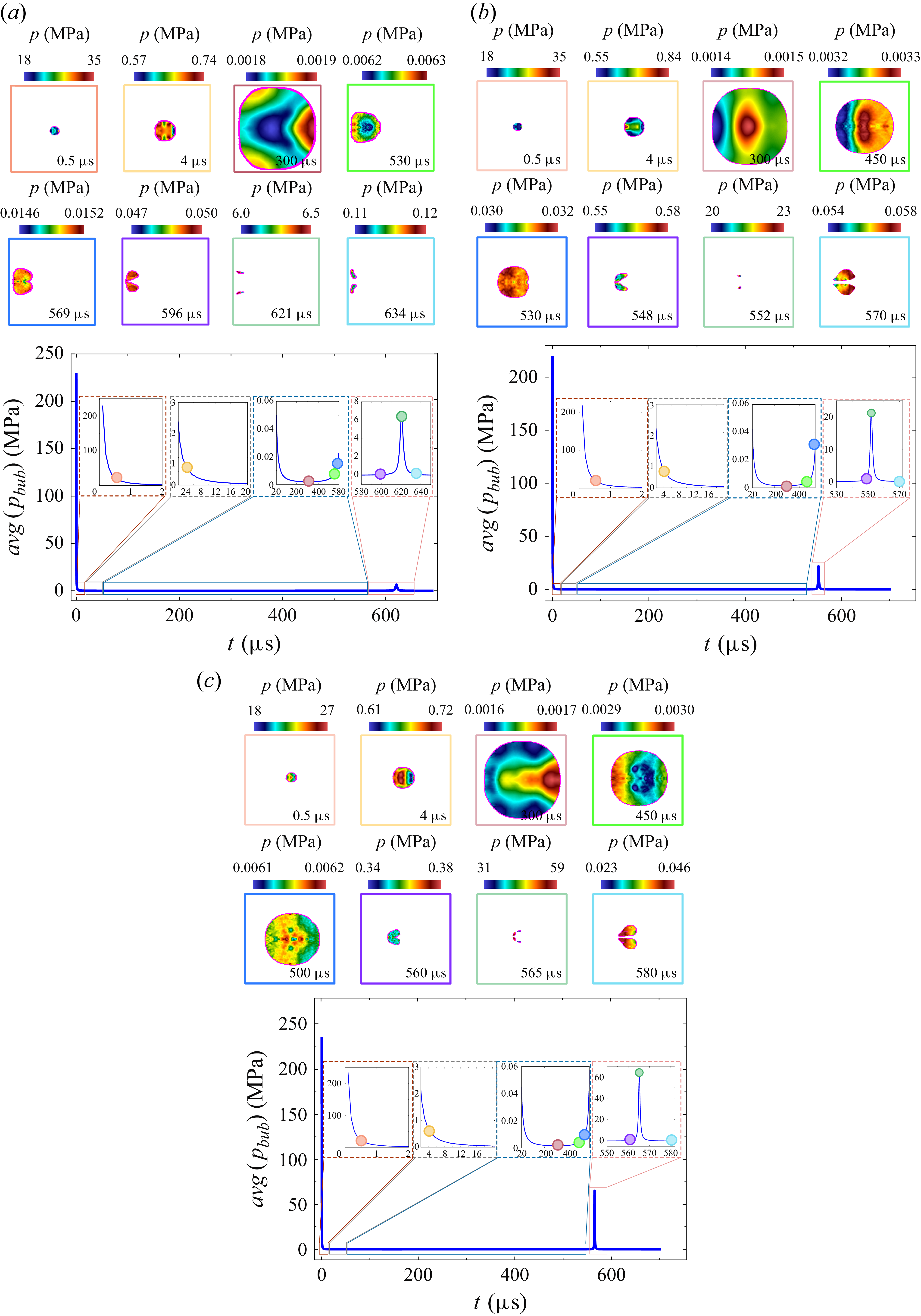
 avg(Pbub)
 γ
γ γ
γ γ
γ tc
tc tc
tc μs
μs γ
γ tc
tc μs
μs γ
γ tc
tc μs
μs γ
γ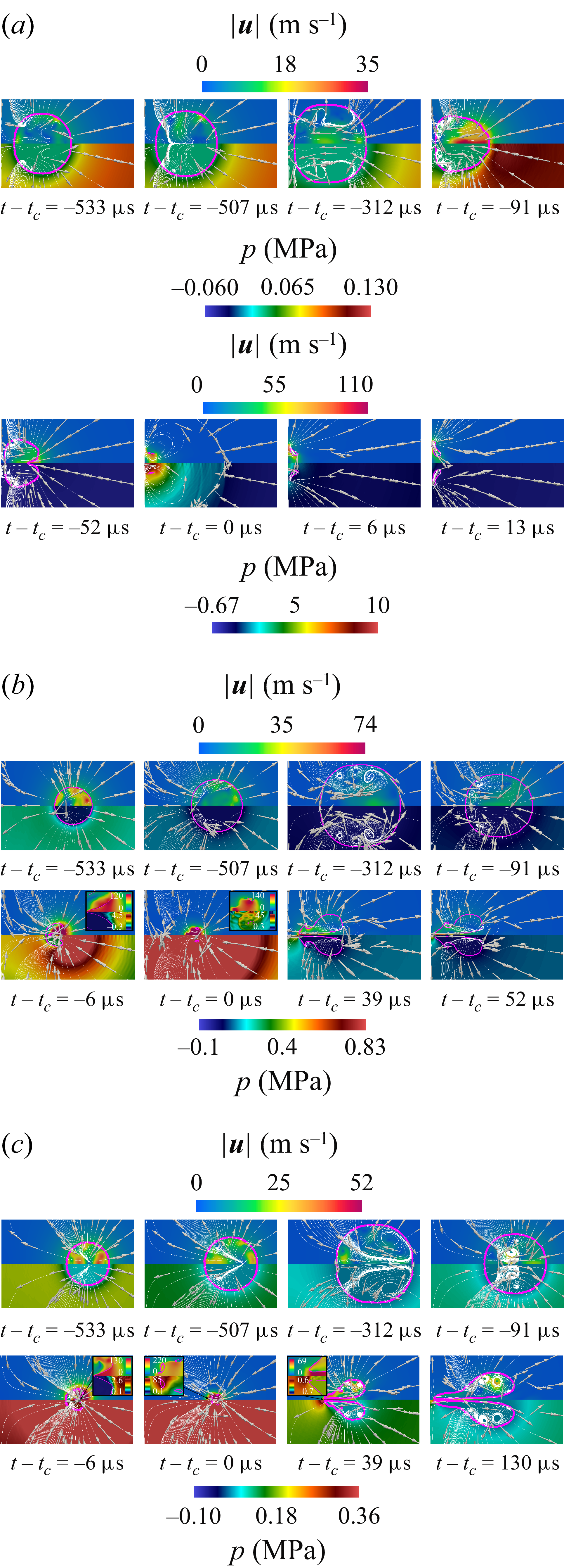
 γ
γ γ
γ γ
γ tc
tc tc
tc μs
μs γ
γ tc
tc μs
μs γ
γ tc
tc μs
μs γ
γ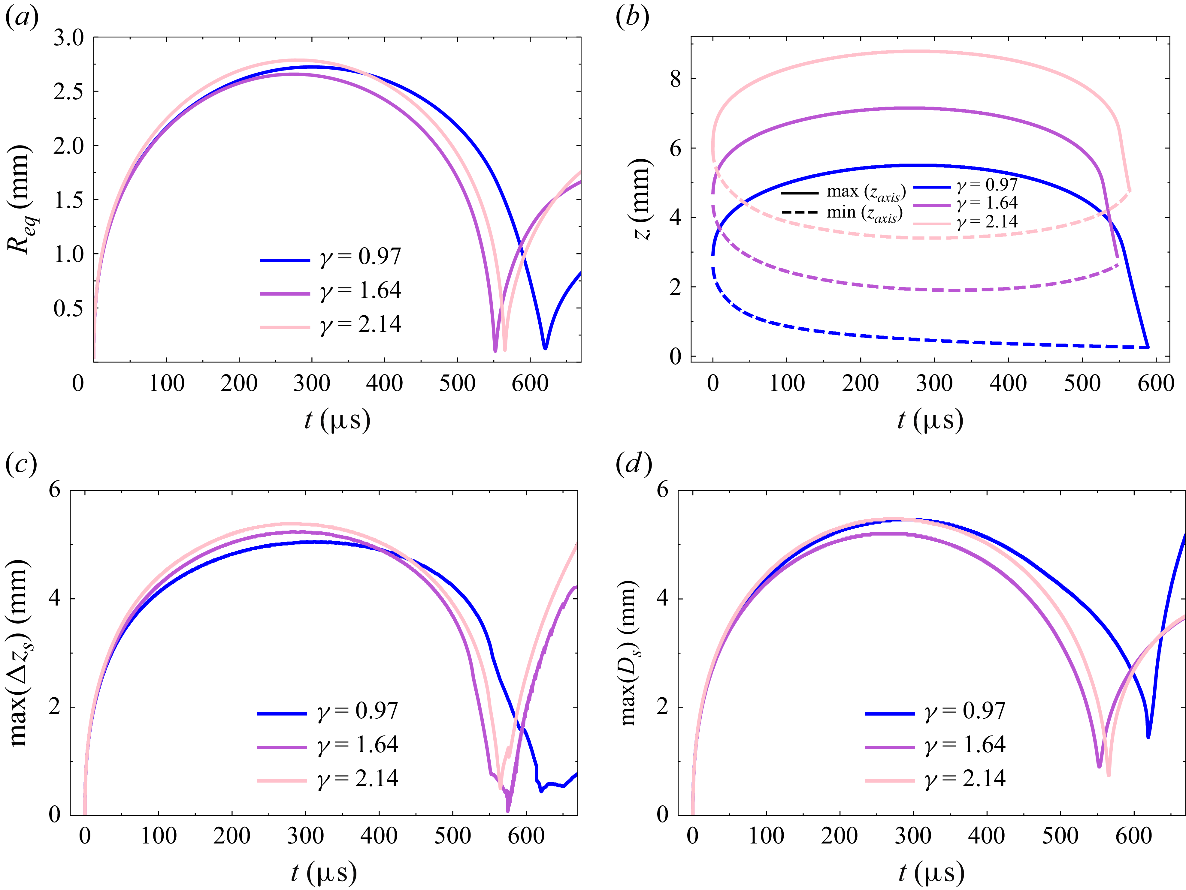
 Req
Req z
z max(Δzs)
 max(Ds)
 γ
γ m−1
m−1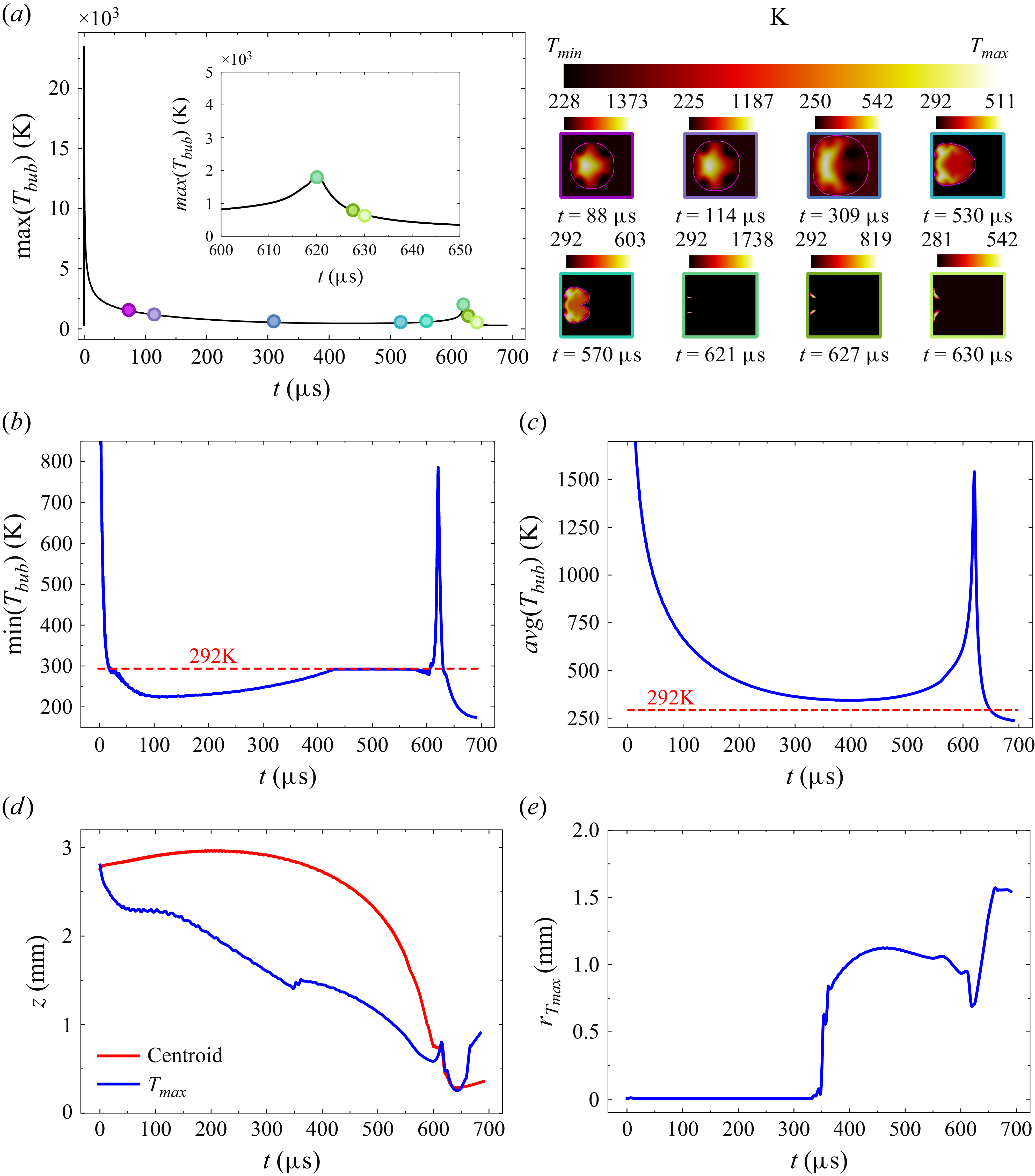
 γ
γ tc
tc tc
tc μs
μs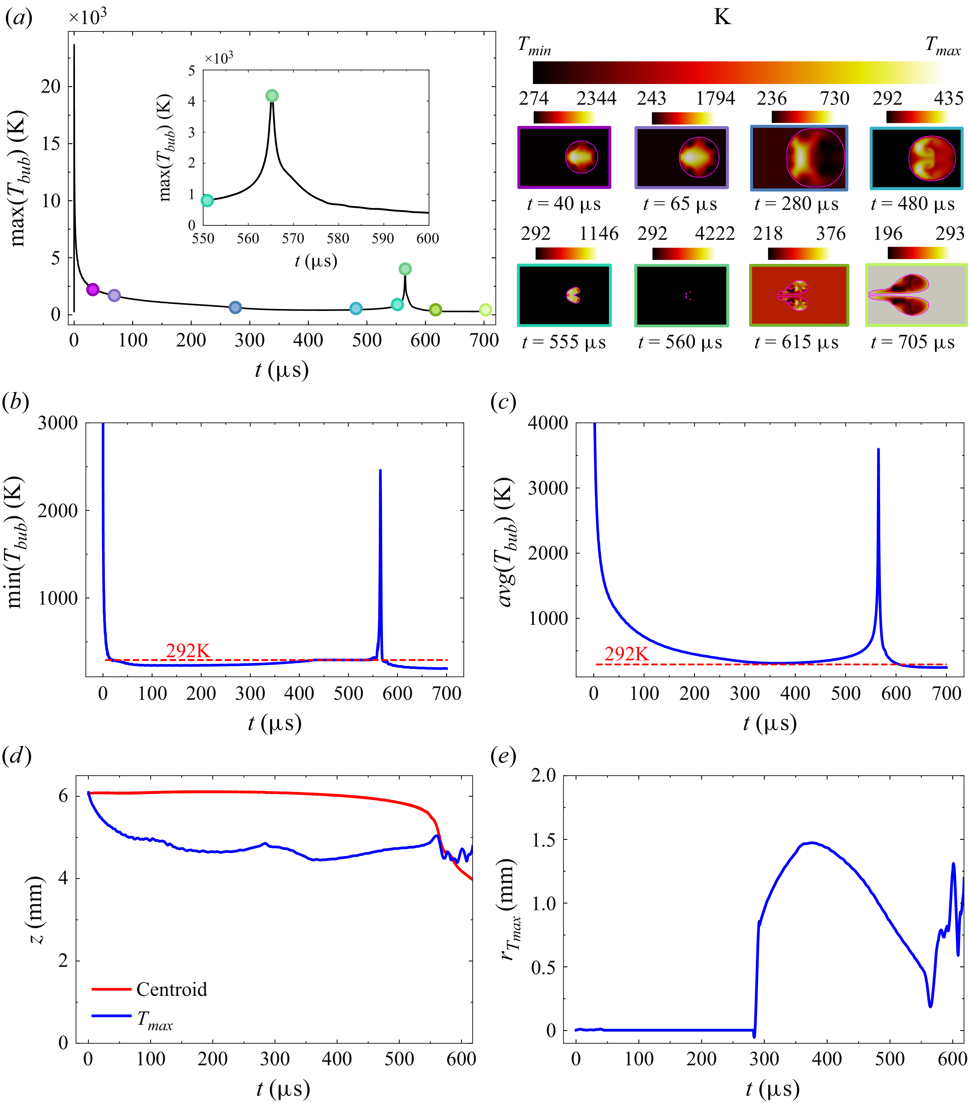
 γ
γ tc
tc tc
tc μs
μs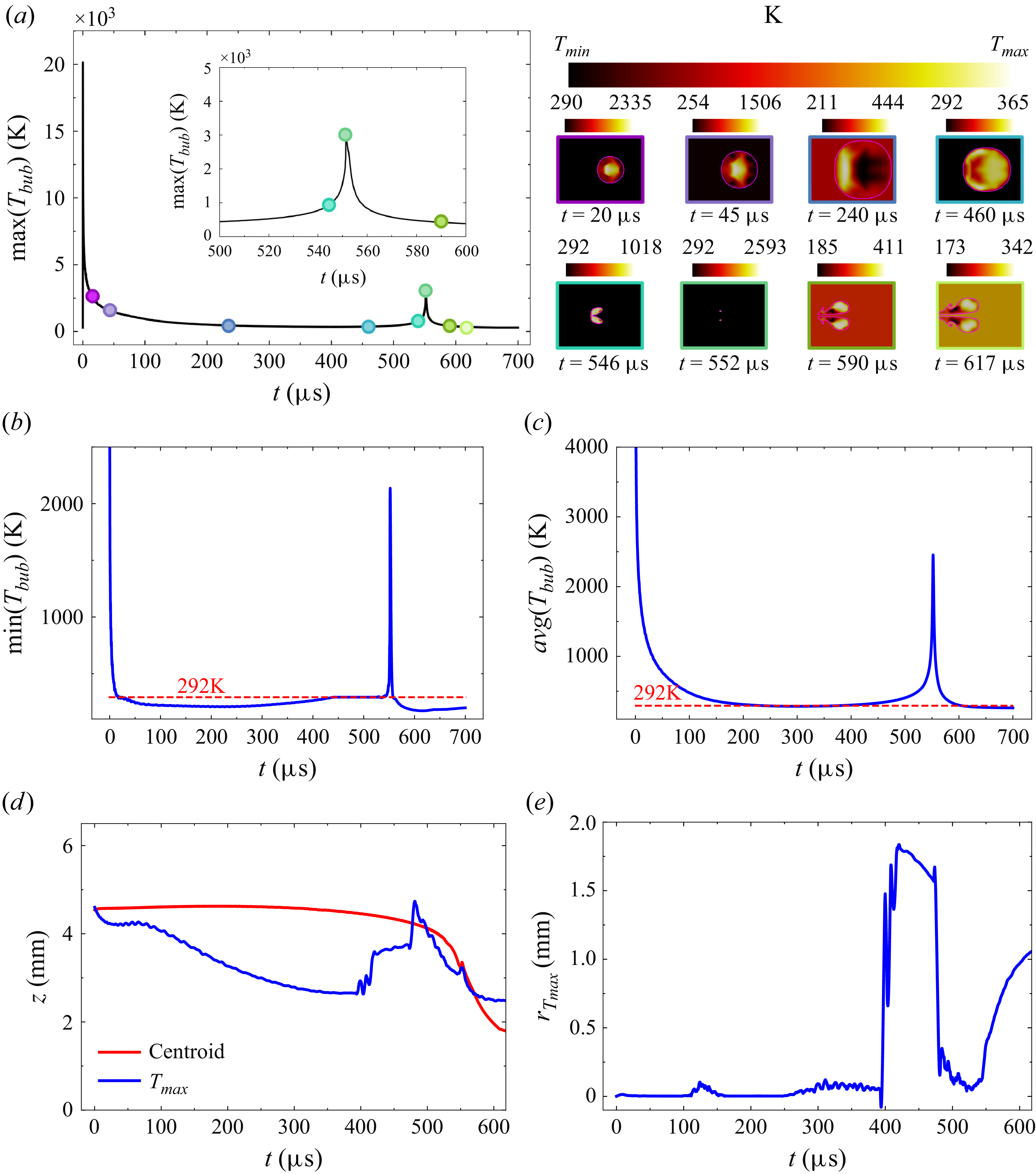
 γ
γ tc
tc tc
tc μs
μs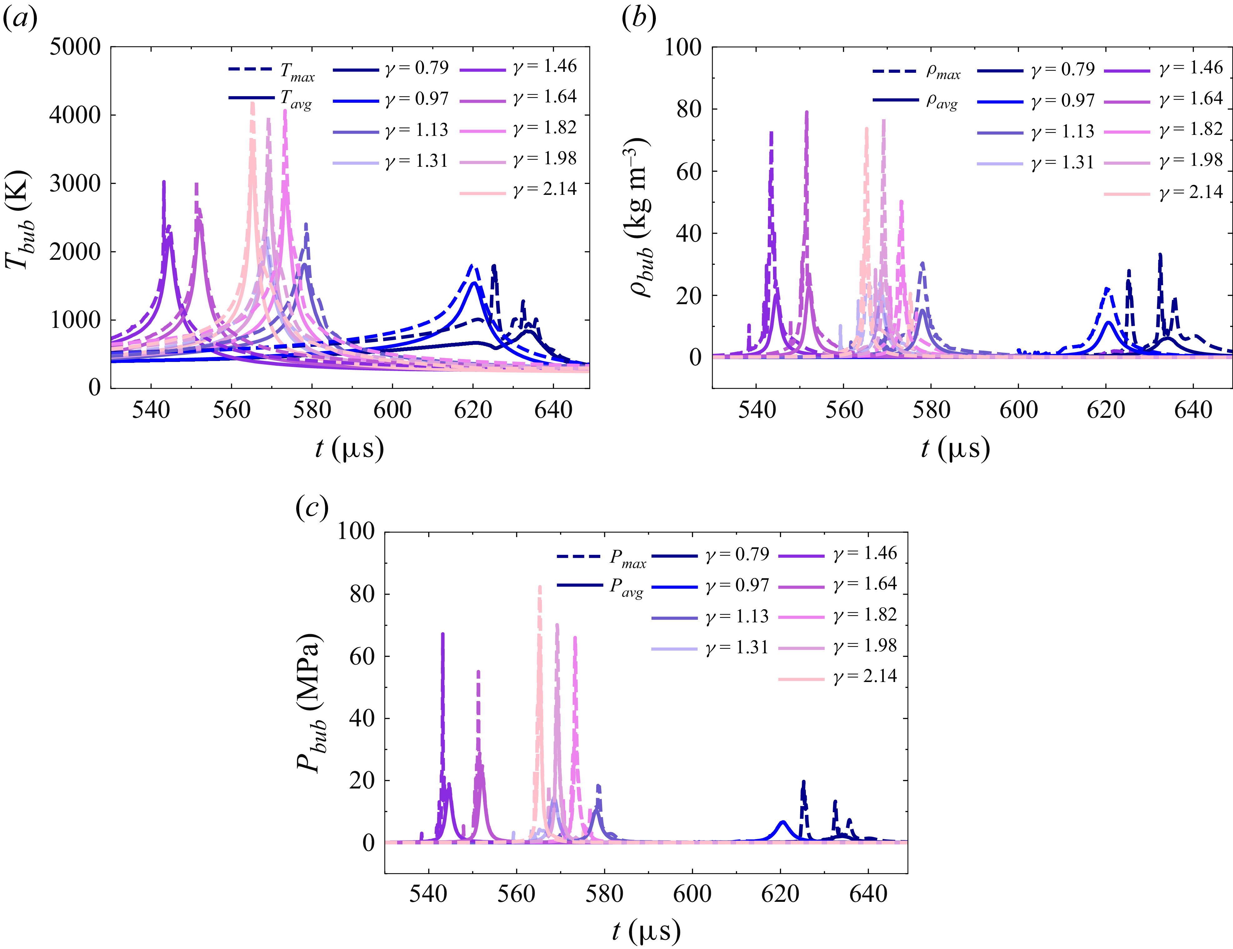
 γ
γ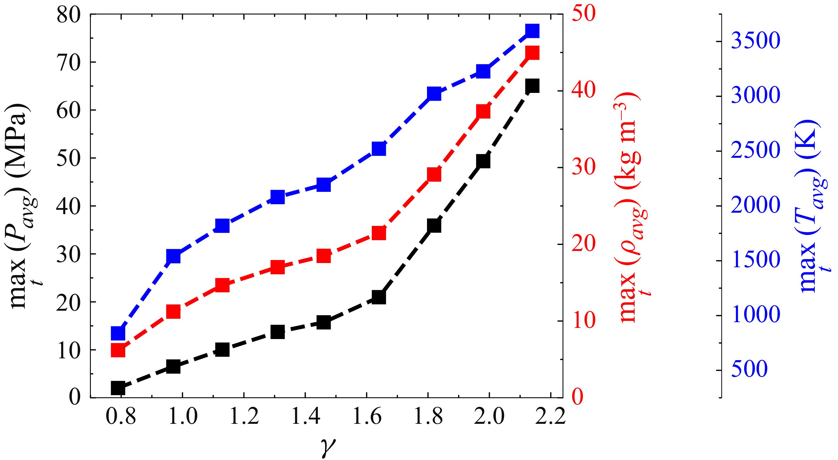
 γ
γ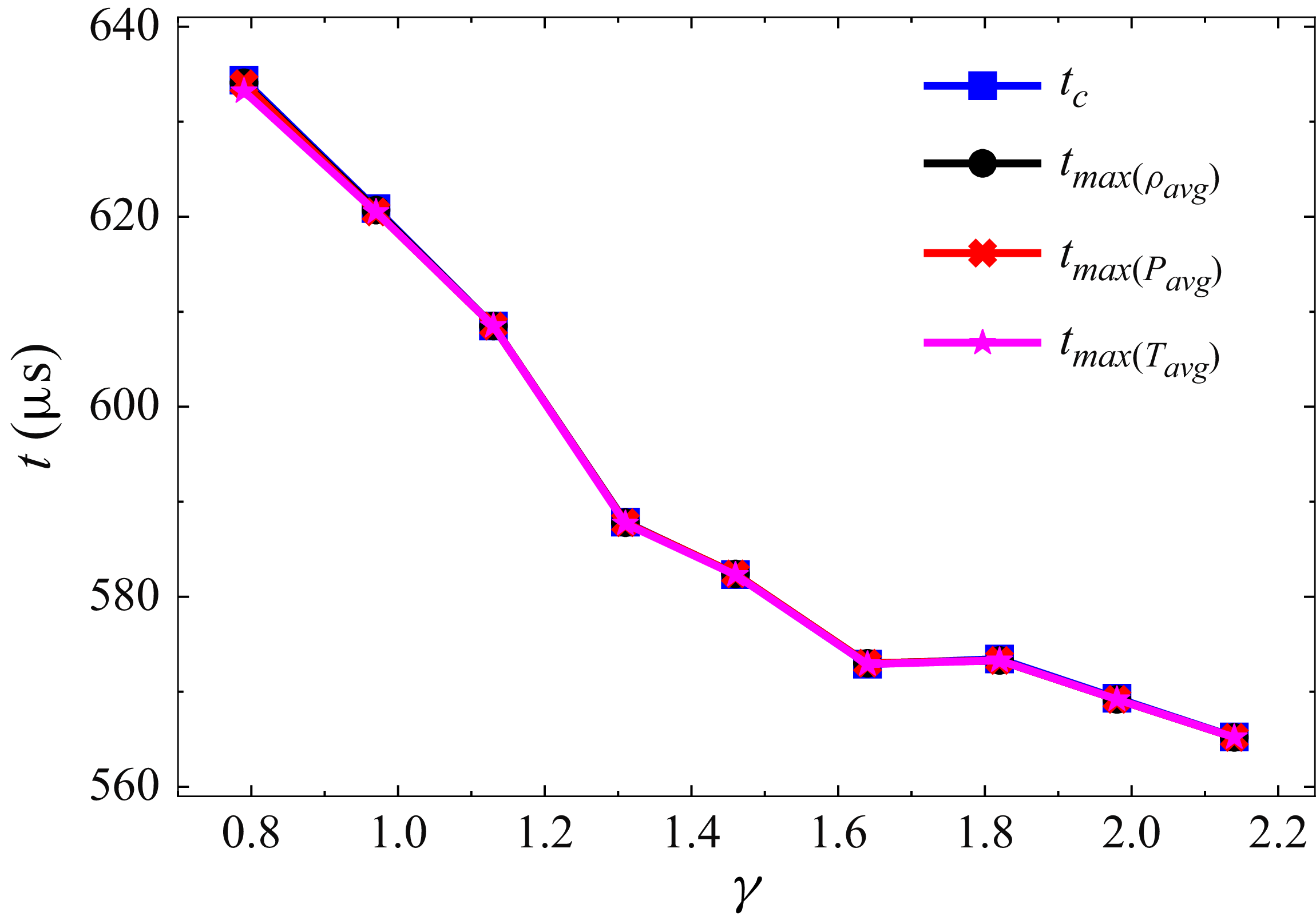
 tc
tc tmax(Pavg)
 tmax(ρavg)
 tmax(Tavg)
 γ
γ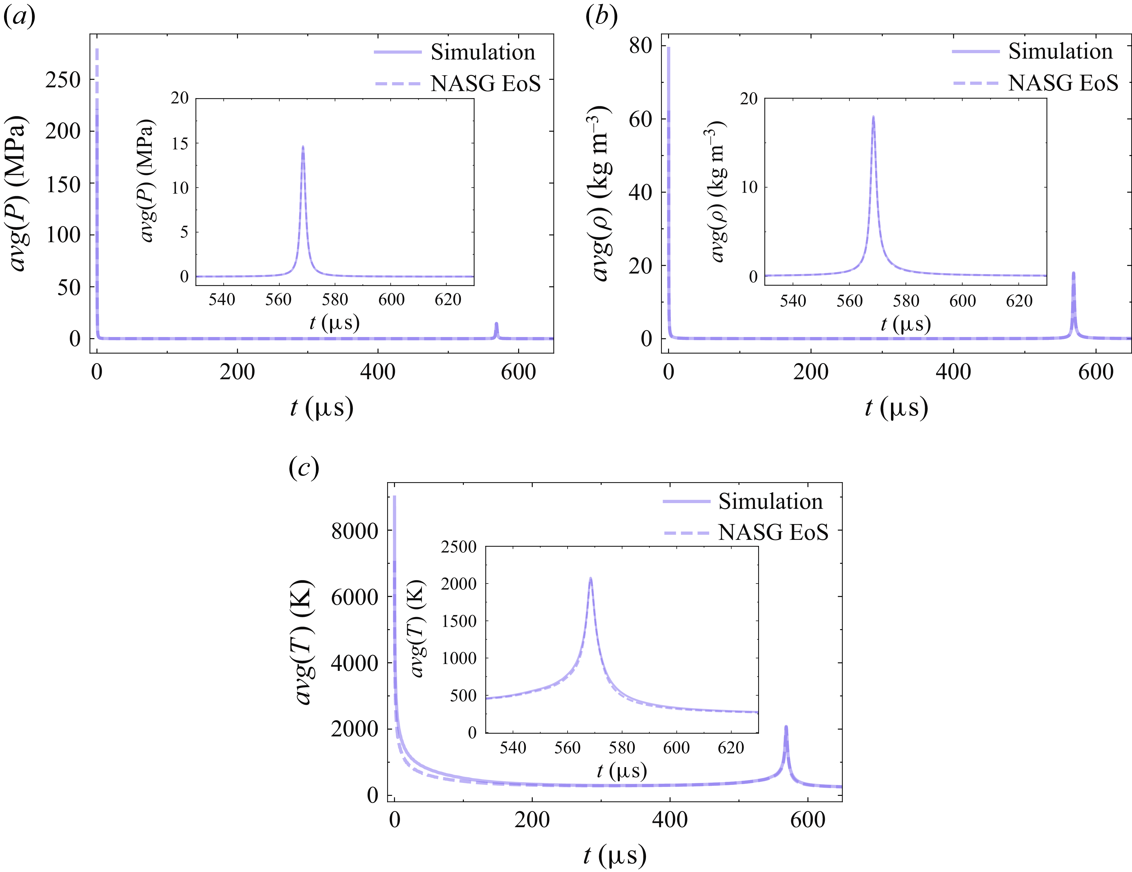
 γ=1.31
 μs
μs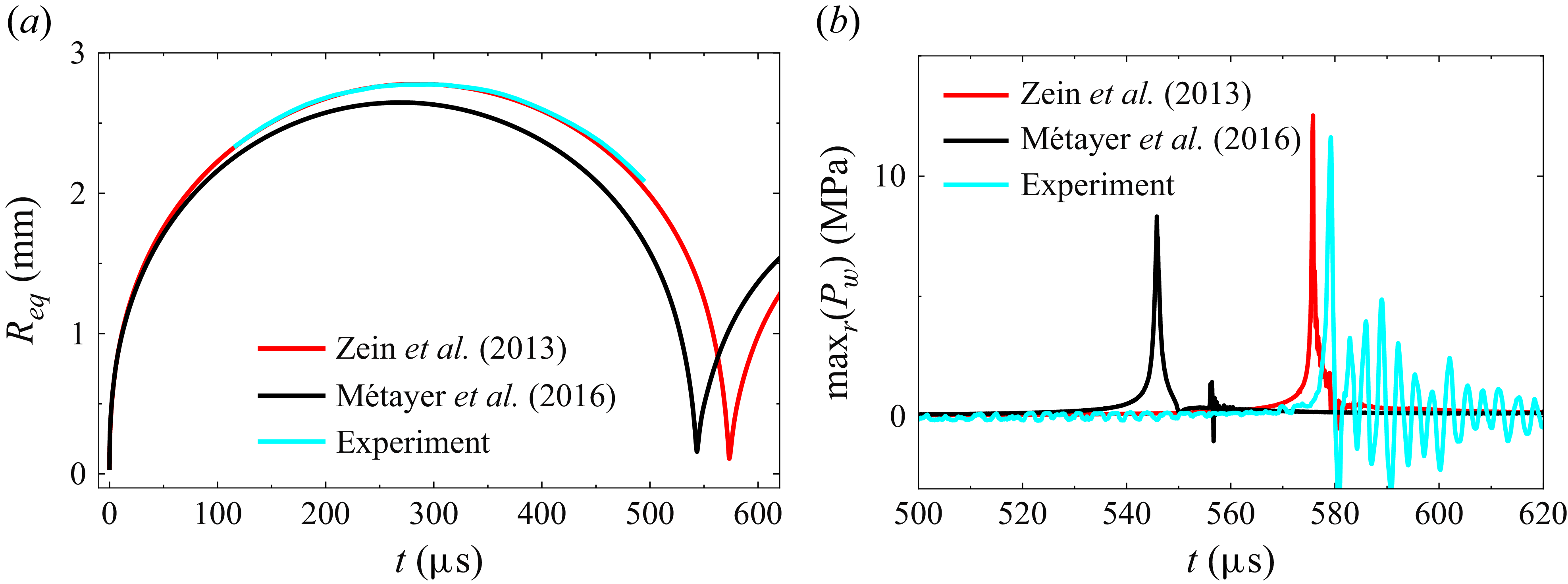
 γ=1.82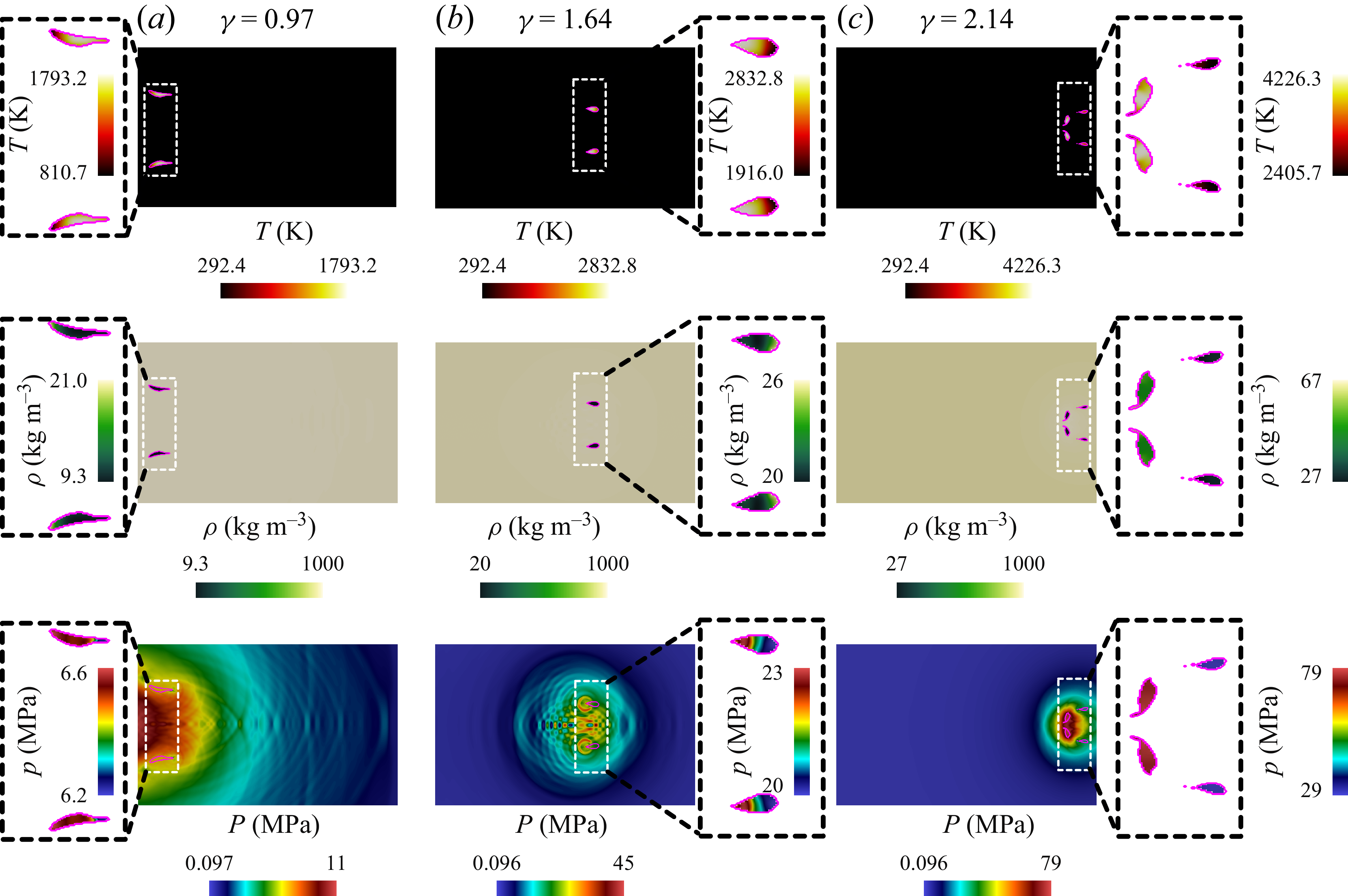
 γ
γ γ
γ γ
γ tc
tc tc
tc μs
μs γ
γ tc
tc μs
μs γ
γ tc
tc μs
μs γ
γ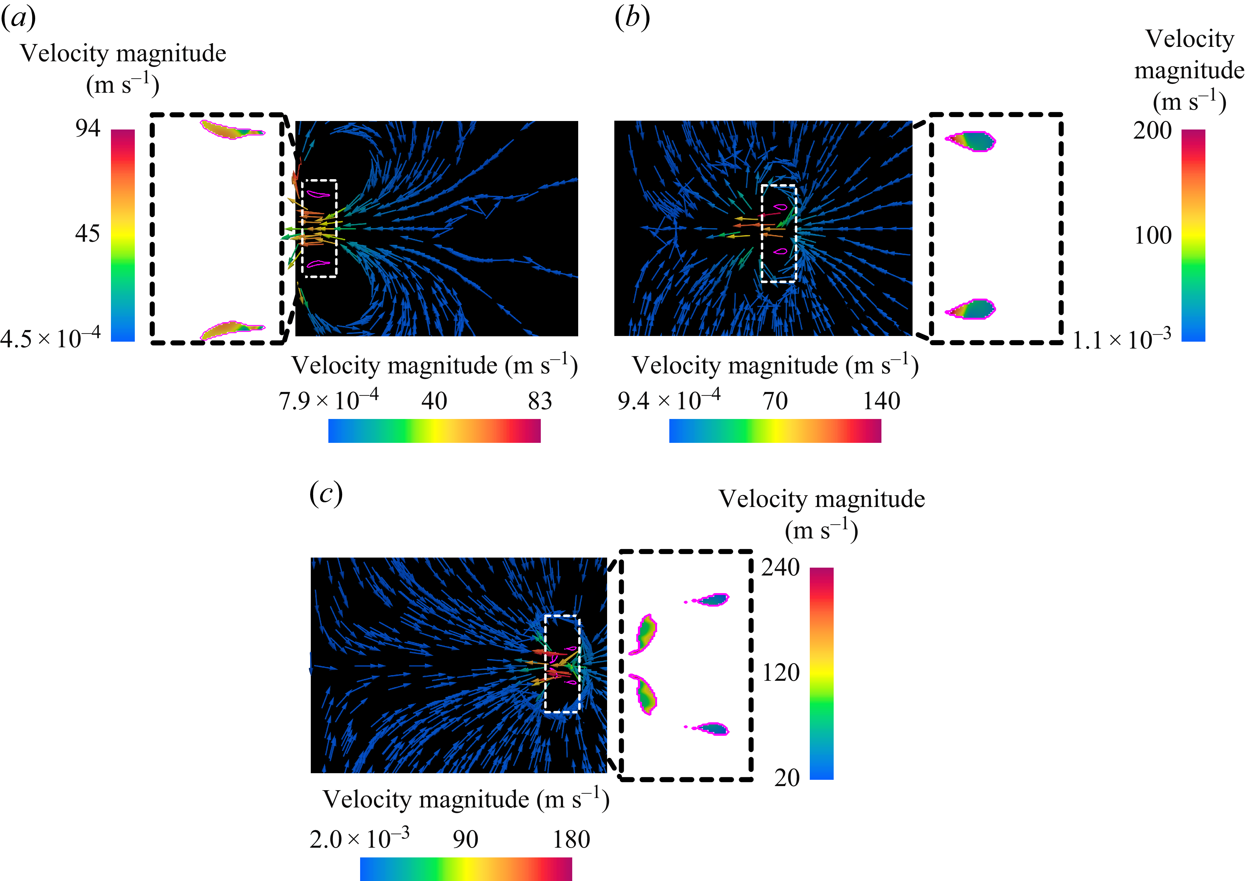
 γ
γ γ
γ γ
γ tc
tc tc
tc μs
μs γ
γ tc
tc μs
μs γ
γ tc
tc μs
μs γ
γ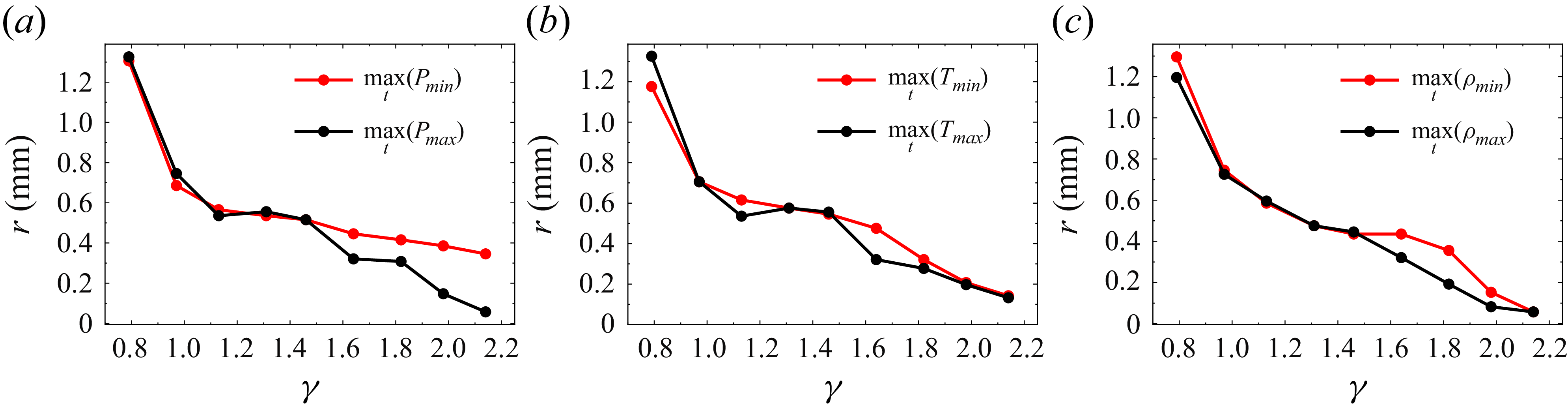
 γ
γ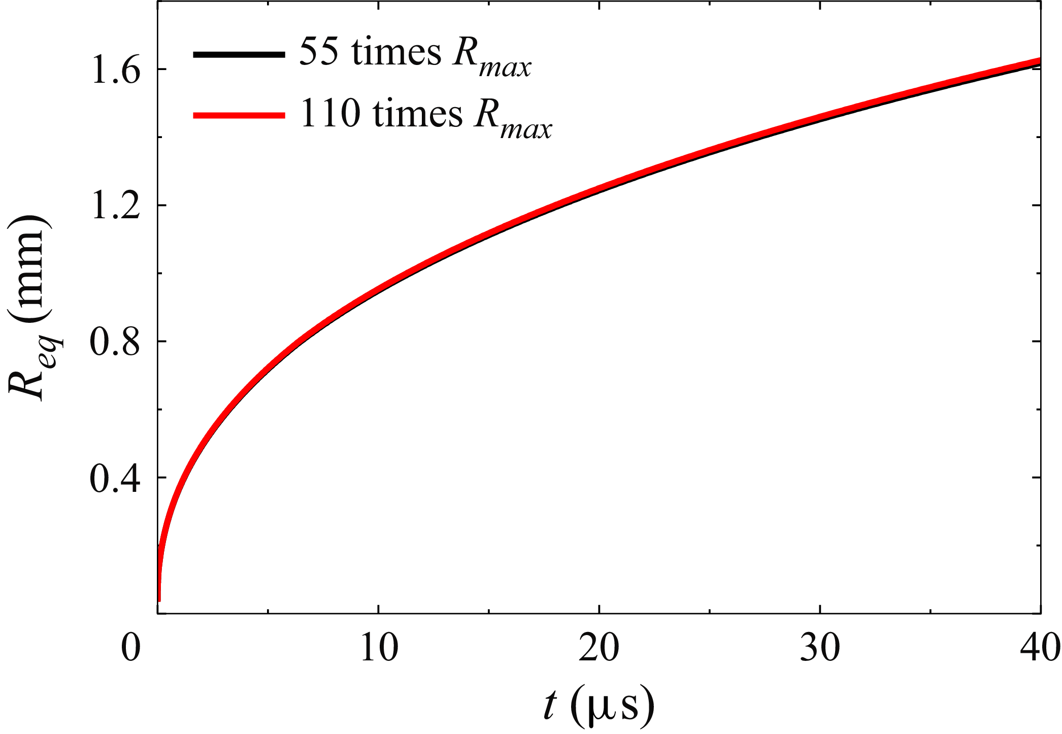
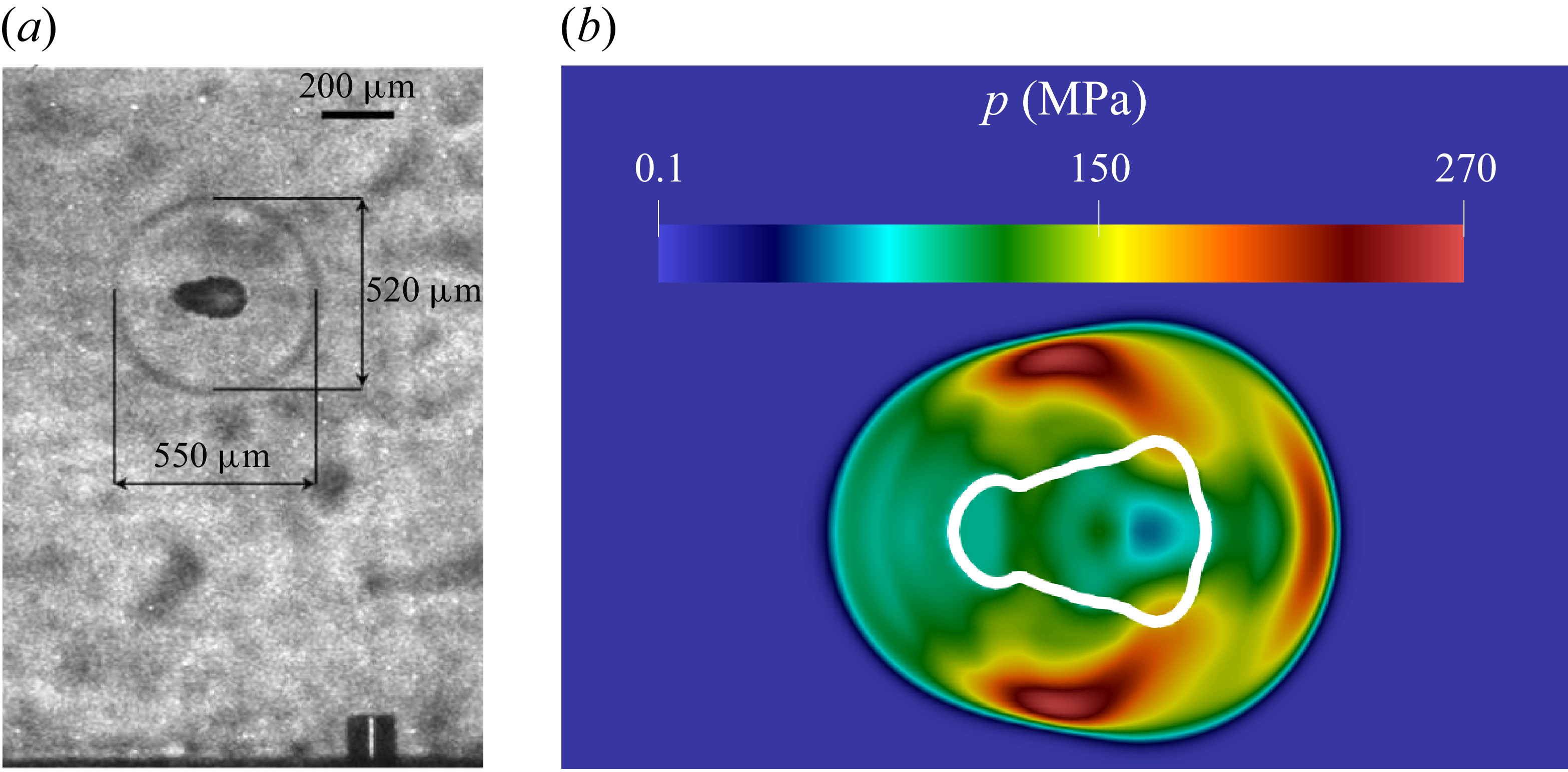
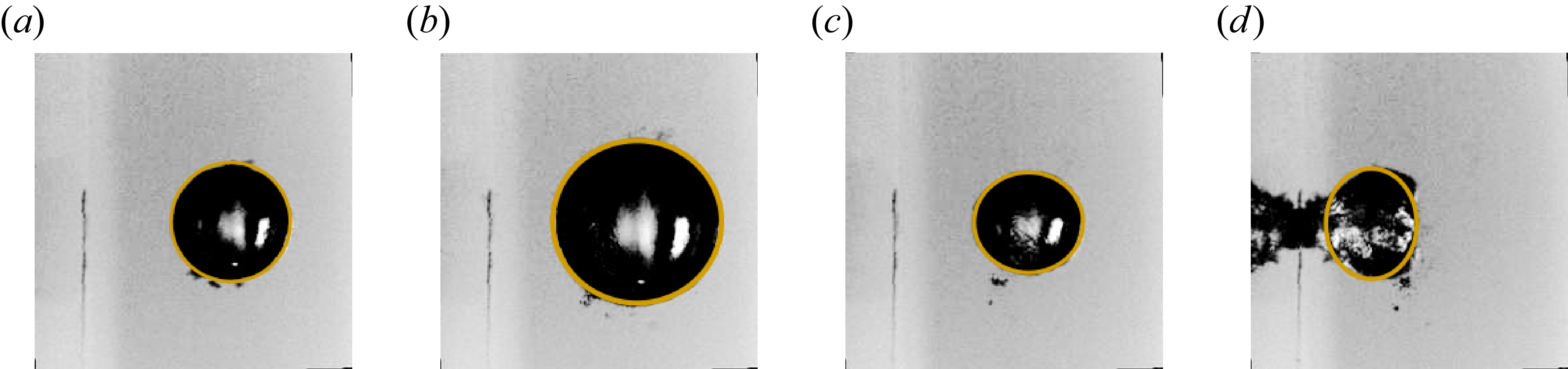
 γ=1.64
 μs
μs μs
μs μs
μs μs
μs tc=572μs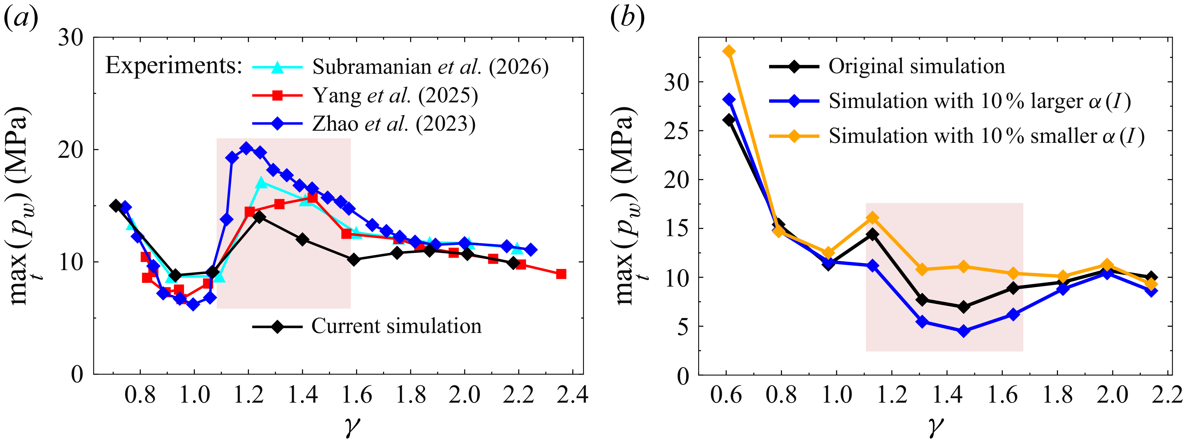
 maxt(pw)
 γ
γ α(I)
α(I)


 Open access

