


1. Introduction
Laboratory experiments are performed to study the intrusion of solitary waves and undular bore into a channel from a wide basin. The set-up for the experiments is considered to be an idealized model for a tsunami intrusion into a river. In the laboratory model, the shoreline is a vertical wall eliminating the process of run-up on a sloping beach; the river channel is idealized as a flat-bottom rectangular channel neglecting the processes of wave propagation up a sloped and winding river channel; the ocean is modelled as flat bottom neglecting any variation in the ocean floor; the incident wave approaches normal to the shore, i.e. in the opposite direction to the outflow from the channel. Those choices focus the investigation to the effects of wave interaction with the current of a finite breadth, and wave intrusion processes due to the geometric transition from basin to channel.
The present study is motivated by some field observations of tsunami intrusion into the rivers. Tsunami behaviours during river intrusion have been explored previously, such as tsunami waveform changes due to tidal phase (Kalmbacher & Hill Reference Kalmbacher and Hill2015; Shelby, Grilli & Grilli Reference Shelby, Grilli and Grilli2016), river surface slope and riverbed slope (Tolkova, Tanaka & Roh Reference Tolkova, Tanaka and Roh2015; Tanaka et al. Reference Tanaka, Tinh, Hiep, Kayane, Roh, Umeda, Sasaki, Kawagoe and Tsuchiya2020), and changing wave height during intrusion (Kakinuma & Kusuhara Reference Kakinuma and Kusuhara2022), among others. To our knowledge, no previous laboratory study has been reported to explore the basic mechanisms for the intrusion of isolated waves into the flow-discharging channel. Because a solitary wave is a stable and permanent-form wave, it is convenient to use solitary waves in laboratory experiments. Though solitary waves frequently serve as models of tsunamis, it must be cautioned that there are differences between idealized and real tsunamis (see e.g. Hammack & Segur Reference Hammack and Segur1978; Yeh, Liu & Synolakis Reference Yeh, Liu and Synolakis1996; Madsen, Fuhrman & Schäffer Reference Madsen, Fuhrman and Schäffer2008).
Unlike solitary waves, an undular bore is not a permanent-form wave, and continually changes its form. Based on the Korteweg–de Vries equation, Gurevich & Pitaevskii (Reference Gurevich and Pitaevskii1974) show that undulation grows and expands in space and time, and the leading undulation emerges as a solitary wave with the amplitude twice the bore height; this process continues to form and emerge a succession of solitons in front of the bore. The prediction of the unsteady behaviour is further refined with the higher-order theory: for example, the analysis based on the Su–Gardner equation by El, Grimshaw & Smyth (Reference El, Grimshaw and Smyth2006).
Wave–current interaction is a classic problem that has been studied for decades (e.g. Peregrine Reference Peregrine1976; Jonsson Reference Jonsson1990; Zhang et al. Reference Zhang, Simons, Zheng and Zhang2022). For solitary waves, Nakayama et al. (Reference Nakayama, Tani, Yoshimura and Fujita2022) demonstrated agreement between numerical and laboratory experiments on the effect of vorticity in the vertical plane on solitary-wave profile and energy. Umeyama (Reference Umeyama2013, Reference Umeyama2019) measured the velocity profiles under solitary waves with and without currents. There are theoretical models (Benjamin Reference Benjamin1962; Freeman & Johnson Reference Freeman and Johnson1970; Choi Reference Choi2003) and numerical experiments (e.g. Pak & Chow Reference Pak and Chow2009; Duan et al. Reference Duan, Wang, Zhao, Ertekin and Yang2018; Yang & Liu Reference Yang and Liu2022) describing the effect of currents on solitary waves. Furthermore, solitary-wave-induced currents have received some attention in the laboratory. Ting (Reference Ting2006, Reference Ting2008) provides a detailed description of the flows generated under a breaking solitary wave on a plane beach. Combined solitary waves and steady currents have been investigated for their effect on structures (Velioglu Sogut, Sogut & Farhadzadeh Reference Velioglu Sogut, Sogut and Farhadzadeh2021; Yang et al. Reference Yang, Huang, Kang, Zhu, Han, Yin and Li2021) and sediments (Sogut, Velioglu Sogut & Farhadzadeh Reference Sogut, Velioglu Sogut and Farhadzadeh2022). Additionally, laboratory experiments for the interactions of undular bore and current have been studied from the perspective of open channel flow through the analogous case of undular hydraulic jump (Chanson (Reference Chanson2009) and the references therein).
A majority of the previous studies dealt with the interactions of solitary wave and current in the vertical plane, while the study of interactions with the current of a finite horizontal breadth is rare. Nonetheless, there are some studies relevant to the present problem. For example, transmission of waves through a gap between two basins was studied in the context of solitary waves by Lynett et al. (Reference Lynett, Liu, Losada and Vidal2000). They found that the wave amplitude through the gap is larger than the offshore condition due to diffraction from the reflective walls adjacent to the gap. Note that the present problem is on wave intrusion into a channel, instead of expanding into the other wide basin. Winckler & Liu (Reference Winckler and Liu2015) showed numerically that solitary waves in smoothly converging channels focus the wave energy during the transition.
For converging channels, tidal motion can generate undular bores (i.e. tidal bores) in the channel (e.g. Bonneton et al. Reference Bonneton, Bonneton, Parisot and Castelle2015). In the case of undular tidal bores, the waves evolve from smooth tidal motions at the estuary outlet into an undular bore over the convergence length of the estuary, whereas undular-bore-like tsunamis can occur in the continental shelf of the ocean and/or during shoaling before reaching the shore (e.g. Knowles & Yeh Reference Knowles and Yeh2020). The abrupt transition from basin to channel lies somewhere in between the former conditions, where the wave energy may be reflected back into the basin, but waves transmitted through the transition remain confined in the channel. This behaviour was examined for solitary waves and a bore-shaped wave transitioning from basin to channel for composite geometries in the still-water condition with numerical experiments by Kakinuma & Kusuhara (Reference Kakinuma and Kusuhara2022).
In this study, the laboratory apparatus is first described in § 2. The apparatus is designed specifically to achieve a steady shallow-water jet suppressing meandering formation in the basin. The performance of the outflowing jet in the basin is presented in § 3. Interaction of incident solitary wave with the jet in the basin and subsequent transition into the channel are discussed in § 4.1, followed by the case of the incident undular bore in § 4.2. Then we summarize the results and state the conclusions in § 5.
2. Experiments
Experiments are performed in a water-wave tank that is 7.3 m long, 3.6 m wide and 0.30 m deep; the tank is elevated 1.2 m above the laboratory floor, as depicted in figure 1. The bottom and sidewalls are constructed of 12.7 mm thick glass plates. This equipment facilitates the use of optical techniques to measure wave and flow fields. The wave tank is equipped with a piston-type wavemaker along the headwall, capable of generating arbitrary-shaped waves with an array of sixteen linear motors. The maximum horizontal paddle stroke is 55 cm, sufficient to generate very long waves in water depth  $h_0 = 5.0\,{\rm cm}$ that is used in the present experiments. Detailed description of the wave tank is available in Li, Yeh & Kodama (Reference Li, Yeh and Kodama2011).
Schematic views of the experimental apparatus (dimensions in m): (a) plan view; (b) elevation view.

A laboratory apparatus is designed for creating a uniform and stable discharge into the shallow-water basin. A carefully controlled shallow-water jet is critical for the study to explore the mechanisms of wave–current interaction. As shown in figure 1, the discharge channel (0.230 m wide and 3.66 m long) and the basin (2.72 m wide and 3.58 m long) are subdivided with vertical partition walls in the wave tank. The channel width was selected to be comparable to the solitary-wave length scales, discussed in § 4.1.3. The channel length is sufficiently long so that a fully developed steady and uniform flow is established from the flow-generating system (see figure 2). The discharge from the channel forms a jet into the basin towards the wavemaker, then splits laterally to the sidewalls near the end of the basin. The sidewalls were punctured with six 2.5 cm diameter holes centred 2.5 cm above the bottom, between 0.8 m and 1.2 m from the wavemaker paddle resting position, to allow the flow through the porous section of the sidewalls and return to the recirculating flow system. For a detailed description of the flow recirculating system, see Salemink-Harry (Reference Salemink-Harry2023).
Flow-generating system: (a) photograph, and (b) schematic of the apparatus.

To create a steady and symmetric discharge in the basin, the discharge rates through the porous sidewall must be identical, and the net return flow from the basin must balance the outflow rate from the channel to the basin. This is accomplished by controlling the flow rate to each intake (see figures 1 and 2) with the use of a dedicated inline pump, rotameter and globe valve. The intake pipes feed into opposite sides of an elevated and vented head tank. The flow out of the head tank is driven by gravity through a manifold at the bottom of the head tank, which splits the flow into five separate discharge conduits. The same flow rate in each discharge conduit is achieved by individually controlling a dedicated inline globe valve and rotameter. The conduits are then connected to a flow-straightening device consisting of five horizontal rigid pipes (0.025 m in diameter and 0.57 m long) that are spaced evenly across the 0.23 m wide channel to create a uniform discharge into the channel. Immediately after the flow exits in the channel, excessive ripples are suppressed by a screen that protrudes from the water surface by a few millimetres. A schematic diagram of the flow-generating system is shown in figure 2(b). This flow-generating system, together with the precision wave tank apparatus and wavemaker system, results in a controlled steady and symmetrical flow field in the basin. The performance of the flow-generating system is presented in § 3.
Measurements of flow velocities at the water surface are made using the particle image velocimetry (PIV) technique. A video camera (AOS Q-PRI with resolution  $1024 \times 1024$ pixels at rate 12.5 Hz) is configured at 1.7 m above the tank with a top-down perspective of the flow. Slightly buoyant spherical particles made from high-density polyethylene (specific gravity 0.97, 3.1 mm diameter) are used as the flow tracers. A matte black background is fitted underneath the glass-bottom tank to create a contrast between the dark background and the white particles. The imaging system is configured for an approximately $1\,{\rm m} \times 1\,{\rm m}$ field of view at the water surface. The particulate images are analysed using the open source software PIVLab (Stamhuis & Thielicke Reference Stamhuis and Thielicke2014; Thielicke & Sonntag Reference Thielicke and Sonntag2021). A similar configuration is used for a qualitative dye study to examine local flow patterns at the channel mouth: a black background to emphasize the green dye (fluorescein), and an imaging system configured for an approximately $0.1\,{\rm m} \times 0.1\,{\rm m}$ view of the water surface.
Measurements of flow velocities beneath the water surface are made using a side-looking acoustic Doppler velocimeter (ADV) sensor (Nortek Vectrino II 2D-3D Sidelooking) mounted to a stepper motor (Hurst Variable Speed Linear Actuator LAS) such that the elevation of the sensor head is controlled. The water is seeded with neutral buoyant particles ( $10\,\mathrm {\mu }{\rm m}$ glass spheres) to ensure measurements in the sampling volume ${\approx }1\,\text {cm}^3$. The sensor was moved between sampling locations to characterize the profile in depth that is possible only due to the highly repeatable experimental configuration.
Measurements of water-surface elevations are made using the planar laser induced florescence (PLIF) technique. An optical system generates a plumb laser-light sheet (less than 1 mm thick sheet and 30 cm of effective width) illuminating fluorescein dye dissolved in the water. A video camera (Photron Mini-AX100) with resolution  $1024 \times 1024$ pixels captures the illuminated vertical plane at 125 Hz. The water surface is identified by finding a maximum gradient of the grey-scale image intensity. The PLIF technique implemented here yields spatiotemporal water-surface variations, and has been proven to yield precise wave measurements successfully in this laboratory environment (for more details, see Li et al. Reference Li, Yeh and Kodama2011; Chen & Yeh Reference Chen and Yeh2014; Ko & Yeh Reference Ko and Yeh2019).
All the foregoing imaging systems are calibrated to remove lens distortion using the radial lens distortion model by Zhang (Reference Zhang2000). The images are rectified with the aid of a calibration board that is co-planar with the laser sheet for PLIF or water surface for PIV. A difficulty associated with the PLIF technique arises from its application for capturing long waves because of its small vertical-to-horizontal scale ratio. This results in insufficient resolution in the vertical direction. To circumvent this difficulty, we repeat PLIF water-surface profiles on approximately 30 cm segments, and make a montage of the multiple-segment profiles to cover a sufficient span of the wave evolution; the overlapping regions of the measurement are combined with a weighted average. This procedure is possible only with a laboratory apparatus that is capable of precise replication, including the stable jet formation. The similar patching technique is also applied to the PIV technique to capture the temporal mean flow field at the water surface.
Hereinafter, all the data are presented in non-dimensional form. Unless otherwise stated, lengths are normalized by the water depth in the quiescent state  $h_0$, and time is normalized by $t_0=\sqrt {h_0/g}$, in which $g$ is gravity; consequently, velocities are normalized by $c_0=\sqrt {g h_0}$. Unless otherwise stated, the experiments are performed in a quiescent water depth $h_0=0.05\,{\rm m}$. As shown in figure 1, we set the coordinates such that $x$ points upstream in the channel from the channel mouth, $y$ points horizontally in the direction normal to $x$, and $z$ points upwards from the bed.
3. Jet flow field
With the flow generation system described in § 2, a steady discharge rate  $Q=0.432$ is introduced into the channel of breadth $b_0 = 4.6$; thus the average flow velocity in the channel is $u_c = 0.094$. The Froude number of the channel flow is $F_d = 0.094$, and the Reynolds number is $R_e = 3300$. Note that this Froude number is realistic for a river discharge to the ocean, and the Reynolds number is sufficiently large so that the flow is turbulent. The channel flow is discharged into the basin as a jet, where the return flow is controlled to keep the water-surface elevation constant, and the jet straight towards offshore with little meandering formation.
Figure 3 shows the time-averaged flow velocity vectors (shown by the arrows) at the water surface in the basin. Measurements of flow velocities are obtained using the PIV technique as described in § 2. The variation of flow speed is shown in colour. The created jet is indeed straight in the  $-x$ direction, with small fluctuations caused by entrainment from the jet edge, and no noticeable meandering is detected in the measured region, $x > -45$.
Jet flow profile in the basin. The time-averaged velocities at the water surface are shown with the arrows, and the temporal standard deviations of the flow speeds are expressed by the colour scale. The data are taken by the PIV technique. A scale arrow representing  $\boldsymbol {u}=(-0.1,0)$ is drawn for reference at $(x,y)=(5,5)$. https://www.cambridge.org/S0022112024011455/JFM-Notebooks/files/Figure_03/Fig_03.ipynb.

For a plane jet, the streamwise velocity profile can be expressed by the Gaussian-shaped profile (e.g. Fischer et al. Reference Fischer, List, Koh, Imberger and Brooks1979)
 \begin{equation} \frac{u}{u_m} = {\rm e}^{-\beta^2 \ln(2)}, \end{equation}
where  $\beta =y/b(x)$ is the scaled transverse coordinate, $b(x)$ is the half-width of the jet, and $u_m(x)$ is the maximum streamwise velocity (at $y=0$). The half-width of the jet, $b(x)$, is determined from the temporal mean profile of the outflow jet by finding the value where $u(x,y=b) = u_m/2$. Figure 4 shows that the measured lateral velocity profiles exhibit the self-similar profile predicted by (3.1) except near the channel mouth $x=-0.4$. Note that the Gaussian-shaped profile was also validated for a shallow-water jet by others (e.g. Dracos, Giger & Jirka Reference Dracos, Giger and Jirka1992; Jirka Reference Jirka1994).
Lateral profiles of time-averaged streamwise surface velocity at  $x=-0.4, -4, -20, -40$ extracted from figure 3. The red solid line shows (3.1). The self-similar lateral profile is evident except at locations very close to the channel mouth $x=-0.4$. https://www.cambridge.org/S0022112024011455/JFM-Notebooks/files/Figure_04/Fig_04.ipynb.

For fully developed turbulent open-channel flows on a horizontal bed, the streamwise component of the velocity profile over the depth can be approximated with the  $1/7$ power law (see e.g. Henderson Reference Henderson1966) of the form
 \begin{equation} \frac{u}{u_s} = z^{{1}/{7}}, \end{equation}
where  $u_s$ is the velocity at the water surface. The flow measured in the channel ( $x=10$) shows good agreement with (3.2), as shown in figure 5, although near the bed, the measured velocity is lower than the prediction (3.2) due to the resolution deficiency associated with the ADV (the strong shear near the bed cannot be resolved with the sampling volume of the ADV, ${\approx }1\,\text {cm}^3$). A similar agreement was found in the basin sufficiently far from the outlet ( $x = -40$). In contrast, the vertical flow profile at $x = -10$ and $-20$ shows a larger flow speed at mid-depth than at the water surface. This is caused by the formation of a secondary current in the transition of the channel discharge into the basin. Some evidence of the secondary current formation is presented in the Appendix, and more details are discussed in Salemink-Harry (Reference Salemink-Harry2023). The secondary currents observed here are unlikely to have directly influenced the wave–current interactions discussed hereinafter due to their small magnitude.
Vertical profiles of streamwise velocity on the centreline ( $\,y=0$) at $x= 10, 0, -10, -20, -30, -40$. e dashed line shows the (3.2) fit to the velocity measured on the water surface. A slightly low value near the bed is caused by the fact that the ADV sampling volume is not small ( ${\approx }1\,{\rm cm}^3$). https://www.cambridge.org/S0022112024011455/JFM-Notebooks/files/Figure_05/Fig_05.ipynb.

4. Results
The following terminology is used to present the results. The entire domain is designated into two regions, namely the ‘channel’ and ‘basin’ as identified in figure 1. For brevity, a set of experiments performed without introducing the flow is termed the ‘no-flow’ case, while the experiments with the discharge from the channel are called the ‘with-flow’ case.
4.1. Solitary waves
With the piston-type wave-generation system, four cases are examined by generating a solitary wave with amplitudes  $a_0 = 0.1, 0.2, 0.3, 0.4$ at the wavemaker; those solitary waves yield the adequate range of nonlinearity effects and wavelengths that are comparable to the breadth of the current (figure 3). If we take the length scale of a solitary wave, $\lambda$, to contain 95 % of the volume of the solitary wave, then $\lambda = 6.70, 4.74, 3.87, 3.35$ for $a_0 = 0.1, 0.2, 0.3, 0.4$, respectively. Following Goring & Raichlen (Reference Goring and Raichlen1980), the wave-paddle motion is controlled to match the depth-averaged fluid velocity in the Lagrangian sense. The higher-order solution for solitary waves given by Tanaka (Reference Tanaka1993) was utilized, i.e. the departure of water surface $\eta$ from the quiescent state is expressed as
 \begin{equation} \eta = a_0 s^2 - \frac{3}{4}\,a_0^2(s^2 - s^4) + a_0^3 \left( \frac{5}{8}\,s^2 - \frac{151}{80}\,s^4 + \frac{101}{80}\,s^6 \right), \end{equation}
where  $a_0$ is the wave amplitude,
 \begin{gather}
\begin{gathered}
s \equiv \operatorname{sech} (\alpha(x - F t)),\quad F = 1+\frac{1}{2}\,a_0 - \frac{3}{20}\,a_0^{2} + \frac{3}{56}\, a_0^{3},\\
\alpha = \sqrt{\frac{3 a_0}{4}} \left(1-\frac{5}{8}\,a_0+\frac{71}{128}\,a_0^{2} \right),
\end{gathered}
\end{gather}
\begin{gather}
\begin{gathered}
s \equiv \operatorname{sech} (\alpha(x - F t)),\quad F = 1+\frac{1}{2}\,a_0 - \frac{3}{20}\,a_0^{2} + \frac{3}{56}\, a_0^{3},\\
\alpha = \sqrt{\frac{3 a_0}{4}} \left(1-\frac{5}{8}\,a_0+\frac{71}{128}\,a_0^{2} \right),
\end{gathered}
\end{gather} $t$ is the time, $x$ is the distance that points in the propagation direction, and $F$ represents the wave propagation speed. With $\eta$ obtained from (4.1), we compute the depth-averaged fluid velocity by $\bar {u} = F \eta /(1+\eta )$, then find the wave-paddle displacement $\xi (t)$ by integrating ${\rm d}\xi /{\rm d}t = \bar {u}(\xi (t),t$). The paddle motions are identical in the no-flow and with-flow cases. This wave-generation algorithm has been proven to generate an accurate and clean solitary wave in the laboratory apparatus used in the present study (see Li et al. Reference Li, Yeh and Kodama2011; Chen & Yeh Reference Chen and Yeh2014; Ko & Yeh Reference Ko and Yeh2018).
Due to physical constraints, the flow near the wave paddles could not be measured, but the flow is small enough to ignore the effect on wave generation. Using a semi-empirical model for a plane jet given by Fischer et al. (Reference Fischer, List, Koh, Imberger and Brooks1979), the flow speed at the centre of the jet at the location of the paddle ( $x \approx -70$) is $|u_m| \lesssim 0.013$. For the flow shown in figure 3, the maximum speed of the jet at the paddle location would be reduced by approximately 85 %. Note that this estimate is the value at the centre of an unobstructed plane jet; the present conditions may be reduced further by the experimental set-up. Furthermore, the jet breadth ( ${\sim }10$) is much narrower than the span of the wave paddle (55.6), such that the influence of the jet on wave generation is both small and local. The deviation in wave generation is considered sufficiently small for the wave behaviour to be controlled by wave–current interaction on the jet in the basin.
4.1.1. Wave–current interactions in the basin
Figure 6 shows the spatiotemporal variation of the wave-surface profile at  $x = -10$ for the with-flow case $a_0 = 0.3$. The water-surface profile in the lateral span $-2.4 < y <+12.6$ is presented in figure 6(a), assuming that the incident wave and the discharging current are symmetric about $y=0$ (the centreline of the jet discharged from the channel). As shown in figure 3 (also in figure 7a), the jet is confined within $|y| \lesssim 5$ at the location $x = -10$, and the flow in $|y| \gtrsim 5$ is small. Figure 6(b) shows the temporal wave profile along the centreline of the jet, exhibiting the deformation from that of a solitary wave with the substantial trailing depression, whereas the temporal profile away from the jet ( $y = 12.6$) shows the symmetrical solitary wave profile with a small trailing positive hump. Note that this small hump is originated from the jet zone as seen in figure 6(a). The converging wave towards the centre of the jet enhances its wave amplitude and is transformed to a non-soliton-shaped waveform. This generates a small wave that emanates obliquely behind the incident wave. The formation of the obliquely trailing wave resembles the features discussed in Yeh et al. (Reference Yeh, Ko, Knowles and Harry2020) for the experiments of a solitary wave perturbed by a submerged narrow sill placed along the propagation direction. This resemblance represents that the effect of the opposing current causes wave refraction in a manner similar to that caused by the depth variation.
Solitary wave profile ( $a_0= 0.3$) at $x=-10$: (a) measured spatiotemporal profile influenced by the opposing current; (b) temporal water-surface profiles, with solid line at $y=0$, and dashed line at $y=12.6$. https://www.cambridge.org/S0022112024011455/JFM-Notebooks/files/Figure_06/Fig_06b.ipynb.

The lateral wave profiles at  $x = -10$: (a) the surface longitudinal speed of the background current $u$; (b) wave amplification ( $a/a_0$); (c) lagged arrival time ( $\Delta \tau$) of the wave crest from the position at $y=12.6$. Note that $\Delta \tau$ is normalized by the time scale of a solitary wave $\tau _0=\sqrt {h_0/g}/(\alpha F)$. https://www.cambridge.org/S0022112024011455/JFM-Notebooks/files/Figure_07/Fig_07.ipynb.

Figure 7 shows the lateral profiles of wave amplitude and phase at  $x=-10$ for the four different solitary waves ( $a_0 = 0.1, 0.2, 0.3, 0.4$); also shown is the profile of background surface current extracted from figure 3(a). The phase presented in figure 7(c) is the time difference $\Delta \tau$ of the wave crest from that passing at $y = 12.6$: here, we normalize the time difference by the time scale of a solitary wave $\tau _0=\sqrt {h_0/g}/(\alpha F)$ that includes the nonlinearity effect given in (4.2a–c). Figure 7(b) indicates that the lateral amplitude profile influenced by the opposing current is essentially independent of the incident wave amplitude (and the wavelength), except for the case $a_0 = 0.1$. It is noted that the amplification away from the zone of the jet is less than unity: as the wave energy is focused onto the jet, there is a corresponding defocusing in the flank. As shown in figure 7(c), the transverse wave phase profiles in the flank of the jet are also independent of the incident solitary waves, once the nonlinearity effect is taken into account, although the phase difference for the case $a_0=0.1$ is smaller than that for larger incident waves. Even at the furthest location, $y = 12.6$, the phase is continually shifting, indicating that the influence of the jet remains present farther away from the jet, though the jet itself is confined in $\vert y\vert \lesssim 5$ (see figure 7a). The slightly different behaviour of the case with $a_0=0.1$ might arise owing to the fact of the longer wavelength associated with that case. The longer incident wave is affected less by the jet with a narrow breadth relative to its wavelength.
Propagation speeds are reduced by the presence of the opposing jet. The wave speed in the basin is computed as the trend of the location of the wave crest in the propagation span  $-20< x<-4$ along the centreline of the jet ( $\,y=0$). The celerity affected by the opposing jet $\Delta c$ is calculated by
 \begin{equation} \Delta c=c-F, \end{equation}
in which the propagation speed under the condition of no background flow  $F$ is obtained from (4.2a–c) and is essentially identical to the measured speed of the no-flow case (see the measured data for $x \lesssim -4$ in figure 12a). The results are shown in figure 8. The dashed line in figure 8 denotes the depth-averaged velocity of the jet along the centreline ( $y=0$), which is estimated from the measured surface velocity $u_s$ (figure 3) assuming that the velocity profile over the depth obeys the $1/7$ power law (see figure 5) as $\Delta c = (7/8) u_s$ with $u_s(x=-20)=-0.0834$. Note that this represents the prediction based on the Doppler effect. An estimate incorporating the entire breadth of the jet as the ratio of momentum to mass flux in the $x$ direction as $\Delta c = M/Q = (4 \sqrt {2}/9) u_s$ is shown with a solid line in figure 8, where $M = \int _0^1 \int _{-\infty }^{\infty } u^2 \,{\rm d}\beta \,{\rm d}z$, $Q = \int _0^1 \int _{-\infty }^{\infty } u \,{\rm d}\beta \,{\rm d}z$, and $u(\beta,z)$ is (3.1) with $u_m$ replaced by (3.2). The solitary waves propagate faster than both estimates.
Influence of the current on the propagation speed along the centreline of the jet ( $\,y=0$): dots show the difference between the measured wave celerity and the undisturbed wave celerity given in (4.3); the dashed line gives the depth-averaged streamwise flow velocity along the centreline; the solid line gives the flow velocity based on the ratio of $x$ direction momentum and mass flux for the shallow jet at $x=-20$. https://www.cambridge.org/S0022112024011455/JFM-Notebooks/files/Figure_08/Fig_08.ipynb.

The results in figure 8 demonstrate that the propagation speeds in the basin ( $x<0$) along the centreline of the opposing current are not controlled by the local current velocity at the centreline. This faster propagation speed along the centreline (at $\,y=0$) than the prediction with the local current speed must be owing to the fact that the wave on the opposing current is hastened by the laterally connected ambient wave that is not influenced by the jet. This behaviour must result from the circumstances considered in the present study: namely, the incident wavelength is comparable with the breadth of the jet. Suppose that the incident wavelength is much shorter than the current breadth. Then the interaction at the centre of the current should cause the Doppler shift by the local flow speed. On the other hand, when the incident wavelength is much greater than the current breadth, the opposing current would cause negligible effect to the wave propagation, unless the Froude number of the opposing current is sufficiently large. In the present experiments, the whole jet acts to reduce the wave speed locally while the wave propagating in the adjacent quiescent water draws the wave forward, such that it propagates at a speed between the bulk jet Doppler shift and the undistributed velocity (i.e. $M/Q < \Delta c < 0$).
The spatiotemporal water-surface profile along the centreline of the channel ( $\,y=0$) for the incident wave with $a_0 = 0.3$ is presented in figure 9 for the no-flow and with-flow cases. The data are taken via the PLIF technique by repeating the experiment discussed in § 2. The results in figure 9 are montages of nine segments covering in the span $-20 < x < 20$. Overall behaviours of the no-flow and with-flow cases are similar, but exhibit some detailed differences. First, although generated with the same wave-paddle motion, the incident wave is greater and the arrival time is later for the with-flow case compared to the no-flow case. The water surface prior to the arrival of the wave is perfectly calm for the no-flow case, whereas some ripples generated by the flow at the upstream end of the channel are propagating in the offshore ( $- x$) direction for the with-flow case in figure 9. For the no-flow case, the reflected wave from the channel mouth appears to be a clean solitary wave with a reduced amplitude, followed by a series of trailing waves with gradually reducing amplitude and phase speed. For the with-flow case, the reflected wave amplitude is not uniform but modulated by a small disturbance. This small disturbance appears to move in the inshore ( $+x$) direction; hence it must be originated by the trailing waves formed behind the incident solitary wave as discussed for figure 6. In addition, a relatively large disturbance is present in the channel near the mouth ( $x \gtrsim 0$). In the channel far upstream from the mouth, two distinct trailing waves can be identified for both no-flow and with-flow cases, although the amplitudes of the trailing waves are larger for the with-flow case.
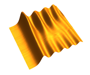
Spatiotemporal water-surface profiles along the centreline of the channel for the incident wave  $a_0 = 0.3$: (a) perspective view, (b) top-down view. https://www.cambridge.org/S0022112024011455/JFM-Notebooks/files/Figure_09/Fig_09.ipynb.

Figure 10 shows the amplitude variations of the incident and reflected waves along the centreline of the channel in the basin for the case  $a_0=0.3$. Even though the incident wave is created with the exactly identical wave-paddle motion, the greater incident wave amplitude $a_i \approx 0.38$ (at $x=-10$) results due to the influence of the opposing current, whereas the amplitude for the no-flow case is $a_i = 0.285 < a_0$ due to the attenuation by friction. On the other hand, the amplitude of the reflected wave $a_r$ for the no-flow case gradually increases as it propagates back to offshore, because of the energy convergence by diffraction from the adjacent waves reflected from the shoreline wall. For the with-flow case, the reflected wave amplitude is modulated, and it does not show an increasing trend in amplitude in $x < -10$: figure 10(b) shows a subtle decreasing trend after some distance away from the shore. In comparison with the incident wave, the reflected wave for the no-flow case is greater than that for the with-flow case. The reflection coefficient ( $K_r = a_r/a_i$) measured at $x = - 10$ is 0.72 for the no-flow case, and 0.57 for the with-flow case. The smaller value of the reflection coefficient for the with-flow case is consistent with the effect of the current: the wave amplifies by the opposing current, while the amplitude reduces by the flow in the same direction as the reflected wave propagation.
Amplitude variations in the basin for the solitary wave with  $a_0=0.3$ along the centreline ( $\,y=0$), with a solid line for the incident wave, and a dashed line for the reflected wave: (a) no-flow case, (b) with-flow case. https://www.cambridge.org/S0022112024011455/JFM-Notebooks/files/Figure_10/Fig_10.ipynb.

4.1.2. Transition from the basin to the channel
To examine the detailed wave intrusion process, a series of water-surface snapshots along the centreline is presented in figure 11 by extracting the data from figure 9. For the no-flow case (figure 11a), the incident wave is a ‘clean’ solitary wave as anticipated. When the wave enters the channel, the waveform becomes asymmetric at  $x=0$, exhibiting the forward tilt. Even after the wave intrudes into the channel, the profile remains asymmetric for some distance, followed by the formation of a long positive trailing hump. On the other hand, for the with-flow case (figure 11b), the incident wave does not exhibit the exact profile of a solitary wave, but forms a large trailing depression due to the influence of opposing current, as shown in figure 6. Contrary to the no-flow case, the wave profile at $x=0$ exhibits a slightly backward tilt because the trailing depression influences the profile. Once the wave enters the channel, unlike the no-flow case, the waveform does not exhibit a pronounced asymmetric profile; the intruded wave quickly becomes close to that of a solitary wave. The difference in profile evolution between the with-flow and no-flow cases is caused by the different wave-reflection and diffraction processes from the neighbouring vertical shore walls, as will be discussed later in this section.
A series of water-surface profiles along the centreline of the channel: (a) no-flow case, (b) with-flow case. A time step 5.60 between subsequent profiles is chosen. The theoretical profile (4.1) of a solitary wave is overlaid with a dashed line in the offshore location. https://www.cambridge.org/S0022112024011455/JFM-Notebooks/files/Figure_11/Fig_11.ipynb.

Figure 12 presents the variation of propagation speed of the incident wave with  $a_0=0.3$ along $y=0$ that is calculated by tracing the location of the wave crest from figure 9. Note that the thin horizontal line in the figure is the predicted propagation speed of the solitary wave, i.e. $c = F$ (see (4.2a–c)). For the no-flow case (figure 12a), the measured propagation speed coincides with the prediction $F$ in the basin, and is slightly higher in the channel due to the increased amplitude. In contrast, the speed of the with-flow case (figure 12b) is slightly lower than the prediction in the basin, and more so in the channel, where it is slowed by the opposing current. The celerity is further reduced in the channel where the flow is essentially uniform across the channel, even though the wave amplitude is larger there. Unlike the propagation in the basin, the speed in the channel is no longer hastened by the ambient wave propagating in the region unaffected by the opposing current.
Propagation speed along the centreline of the channel for the solitary wave with  $a_0=0.3$, where the thin line shows the predicted solitary-wave celerity: (a) no-flow case, (b) with-flow case. https://www.cambridge.org/S0022112024011455/JFM-Notebooks/files/Figure_12/Fig_12.ipynb.

In the transition, the crest celerity varies locally. The propagation speed decelerates at the channel mouth as shown in figure 12. The speed becomes slowest prior to the wave crest entering the channel for the no-flow case, while the minimum speed occurs at the mouth ( $x=0$) for the with-flow case. This behaviour is observed for all of the cases with $a_0 = 0.1, 0.2, 0.3, 0.4$. A mechanism for the slow-down in propagation speed at the channel mouth is the lateral disturbance caused by the wave reflected from the adjacent vertical shore wall, which effectively reduces the speed at the entrance. The propagation speed then increases to take a local maximum during the transition into the channel. For the no-flow case, the maximum speed occurs at the channel mouth ( $x=0$), while the maximum happens slightly upstream in the channel for the with-flow case. Oscillation in speed is observed for the flow case in figure 12(b). The difference of transition behaviour in propagation speed is caused by the difference in reflection process at the neighbouring vertical shore walls; this mechanism will be justified later when we discuss the lateral wave profile (figures 14 and 15). It is important to point out that the foregoing complex behaviours in the transition processes are plausible because the wavelength is comparable to the channel breadth. It is anticipated that the reflection from the neighbouring shoreline should not be prominent for the wave intrusion process to the channel if the channel breadth is substantially larger than the incident wavelength.
Amplification processes along the centreline of the channel for the four cases of incident solitary waves ( $a_0 = 0.1, 0.2, 0.3, 0.4$) are shown in figure 13. The values of wave amplification are obtained as the ratio of the measured amplitude $a$ to the amplitude of the incident wave $a_i$ measured at the reference location taken at $x = - 12$. The results in figure 13 show that the incident wave amplifies locally when it enters the channel. The ripples apparent in figure 13(b) are generated at the upstream end of the channel by the flow exiting the discharge conduits (as seen in figure 9). The maximum amplification during the intrusion at the mouth is greater when the flow discharge is present, except for the case with $a_0 = 0.1$: here, the maximum amplification for the no-flow case is comparable with the with-flow case. Regardless of the presence of the background flow, the smaller the incident wave (or the longer the wavelength), the greater the amplification. For the no-flow case, the maximum occurs immediately outside the channel mouth, while it occurs immediately inside the channel for the with-flow case; this difference causes a drop, followed by a rise, in the ratio of with-flow amplitude ( $a_w$) to no-flow amplitude ( $a_n$) as shown in figure 13(c). Although the amplification in the channel after the transition is comparable in both cases, the with-flow amplitude is larger due to the amplification in the basin ( $a_w/a_n \sim 1.3$).
Spatial variations of wave amplification along the centreline of the channel and the jet for the cases  $a_0 = 0.1, 0.2, 0.3, 0.4$: (a) no-flow case, (b) with-flow case, (c) ratio of with-flow ( $a_w$) to no-flow ( $a_n$) amplitudes. The amplification is relative to $a_i$ at $x=-12$. https://www.cambridge.org/S0022112024011455/JFM-Notebooks/files/Figure_13/Fig_13.ipynb.

Figures 14(a,b) show the spatiotemporal variations of the lateral water-surface profiles of the approaching solitary wave with  $a_0 = 0.3$ at $x = - 3.05$ and $-0.508$, respectively. The no-flow and with-flow profiles are shown in figures 14(a i,b i) and figures 14(a ii,b ii), respectively. The wave arrives earlier for the no-flow case than for the with-flow case. At $x = - 3.05$ (figure 14a), the incident and reflected waves can be seen; note that this is a plot of water-surface elevation $\eta$ in the $y$–
$y$– $t$ plane at a fixed $x$ location, so the first wave represents the incoming wave, followed by the second wave that represents the reflected wave from the shoreline wall. At $x = - 0.508$ (figure 14b), the lateral profile exhibits the run-up essentially at the vertical shore wall, hence the incident and reflected waves are not separated at this location. As shown in figure 14(a i), the crest of the incident wave for the no-flow case is straight and parallel in the $y$ direction, while the reflected wave exhibits a phase delay in the region of the channel opening, even though there is no outflow from the channel. The incident wave for the with-flow case (figure 14a ii) is influenced by the jet just as seen in the offshore wave profile in figure 6.
Spatiotemporal contour plots of the lateral wave profile in the basin for the case  $a_0 = 0.3$: (a) $x=-3.05$, (b) $x=-0.508$. Here, (a i,b i) and (a ii,b ii) are measurements for the no-flow and with-flow cases, respectively. The channel sidewalls are located at $y=\pm 2.3$. https://www.cambridge.org/S0022112024011455/JFM-Notebooks/files/Figure_14/Fig_14.ipynb.

As shown in figure 14(b), the water-surface profile of the leading wave close to the shoreline ( $x=-0.508$) exhibits the influence of wave reflection along the vertical shore walls. For the no-flow case (figure 14b i), the crest line along the shore wall is slightly delayed from that of the intruding wave into the channel. This is because the nonlinear effect associated with the wave reflection causes a phase delay, just like that involved in the head-on collision of the identical solitary waves (Su & Mirie Reference Su and Mirie1980; Craig et al. Reference Craig, Guyenne, Hammack, Henderson and Sulem2006; Chen & Yeh Reference Chen and Yeh2014). On the other hand, the crest line in the channel mouth for the with-flow case (figure 14b ii) becomes almost in line with the reflected wave at the shore wall.
The difference between the rising water surface in the transverse direction along the vertical shore wall (measured at  $x=-0.508$) for the no-flow and with-flow cases is evident in figure 15. As expected for the wave reflection at the vertical wall, figure 15(a) shows that the amplitude away from the channel becomes approximately double ( $a\sim 0.6$) the incident wave amplitude for the no-flow case, and the amplitude at the centre of the channel remains approximately at the level of the incident wave ( $a \sim 0.3$). On the other hand, figure 15(b) shows that the amplitude takes the local maximum at $y \approx 3.8$, then the amplitude level gradually decreases leaving the channel mouth; the reduced wave amplitude is due to the focusing of wave energy from the flank onto the jet in the basin. The wave amplitude becomes fairly uniform in the span of the channel breadth: the amplitude is approximately at the level of the incident wave along the centreline of the jet. During the rising process, the water surface maintains an approximately horizontal line along the shore wall, $y\gtrsim 4$, for the no-flow case. On the other hand, the water surface for the with-flow case exhibits positive gradient (increasing in the $y$ direction) throughout the rising process. This indicates that energy is laterally fed towards the channel mouth along the shore wall by diffraction of the progressively reflected wave. Note that the incoming wave in the basin is refracted by the jet, hence it first arrives at the shore wall at a location away from the channel mouth, then successively impacts the wall towards the mouth. Careful observation of the wave ridge of the spatiotemporal contours shown in figure 14(b ii) confirms the foregoing process: the ridge is extended towards the channel mouth with the delay of timing. This wave reflection/diffraction process along the shore wall results in the greater ‘local’ enhancement of the intruded solitary wave when the current is present as shown in figure 13. This wave diffraction mechanism also explains the local variation in propagation speed as shown in figure 12.
Temporal variations of the lateral water-surface profiles at  $x = - 0.508$: (a) no-flow case, (b) with-flow case. Water surface profiles shown in solid lines, channel wall position shown in vertical dashed lines. https://www.cambridge.org/S0022112024011455/JFM-Notebooks/files/Figure_15/Fig_15.ipynb.

Figure 16 shows the temporal variations of lateral water-surface profiles of the four transverse transects for the incident wave ( $a_0 = 0.3$) entering into the channel. The plot at $x=-0.508$ represents the same data as for those in figure 14(b), but plotted for the lateral span of the channel breadth ( $-2.3 < y < 2.3$).
Contour plots of the intruding wave for the case  $a_0 = 0.3$: (a) no-flow case, (b) with-flow case. https://www.cambridge.org/S0022112024011455/JFM-Notebooks/files/Figure_16/Fig_16.ipynb.

For the no-flow case (figure 16a), the water-surface profile shows the concave-up pattern during the rising phase at the entrance ( $x=-0.508$ and $0^+$): the water surface rises at the sidewalls first ahead of the centre of the channel. The water surface recedes from the sidewalls once the wave enters the channel (see $x=0^+$ and $0.5$). Note that the crest is approximately straight across the channel throughout the process. Immediately after the wave enters the channel ( $x = 0.5$), the maximum elevation shifts to the centre of the channel; at the same time, a sharp drop is observed in the water surface at the sidewalls. Soon after (at $x=1.52$), the wave approaches uniformity across the channel.
For the with-flow case (figure 16b), the spatiotemporal variations of water surface are approximately flat near the transition ( $x=-0.508$ and $0^+$). The water surface recedes from the sidewalls, similarly to the no-flow case, after the wave enters the channel ( $x=5.08$ and $x=1.52$). The transition behaviours of both no-flow and with-flow cases are caused by the influence of the adjacent wave in the basin that is amplified by reflection at the vertical shore wall as discussed in figure 15. The successive plots towards upstream show the greater water-surface elevation at the edge of the channel at $x=-0.508$, then soon after, convergence and elevation of the water surface at the centre. The water-surface elevation at the edge of the channel at $x = 0.508$ is lower than that at the outside of the channel $x = - 0.508$. This and the evident dips at the sidewalls at $x=0.508$ are likely caused by the formation of the flow separation at the channel mouth during the intrusion of the wave.
Observation of the receding process for both no-flow and with-flow cases (see figures 16(a i–a iii,b i–b iii) at  $x=-0.508, 0^+, 0.508$) shows the convergence of the flow from the sides. The waves from both sides merge at the middle, resulting in the hump in the rear profile. Note that the strong lateral variability in the intruding wave profile gradually diminishes by $x=5.0$ (not shown here).
4.1.3. Summary and discussion for the solitary wave cases
The following findings for the solitary waves are some key behaviours when the wavelength is comparable to the breadth of the shallow-water jet. First, wave refraction by the opposing current of the finite breadth in the basin causes the deformation of the solitary-wave profile, emerging with a large depression tail and emanating a small oblique trailing wave (figure 6). Though minute, this radiating oblique wave represents a mechanism to disperse the soliton energy; this mechanism was pointed out by Yeh et al. (Reference Yeh, Ko, Knowles and Harry2020) for the similar radiation process due to a submerged narrow sill along the wave propagation. The refraction bends the wave crest line, resulting in focusing energy into the jet, and defocusing in the flank area of the jet. Consequently, the amplitude in the flank becomes smaller than that of the imposed solitary wave. The wave propagation speed at the centre of the opposing jet is faster than that predicted by the Doppler effect based on the local flow speed. This is because the wavelength is comparable to the jet breadth; hence the wave on the jet is affected by the propagation of the ambient solitary wave away from the jet. It may not be the case if the wavelength scale were much smaller that the breadth of the current. The foregoing predictable behaviours are demonstrated quantitatively in the precisely controlled laboratory environment.
Our results show that the wave transmission process into the channel causes amplitude enhancement in the vicinity of the channel mouth by wave energy transmitted laterally along the shore walls toward the channel. Such lateral energy convergence to the channel is demonstrated in figures 14 and 15. The presence of the flow alters the transition process by changing the waveform offshore via refraction, resulting in progressive wave impact on the wall towards the channel, whereas the no-flow case impacts the walls uniformly. The energy convergence to the channel along the shoreline is more effective, and reaches the channel mouth at a different timing for the with-flow case. Figure 17 illustrates the foregoing mechanisms of the transition processes. Note that a solitary wave with the smaller amplitude has the longer wavelength, therefore the increase in water-surface elevation at the transition starts earlier (more offshore location) than the case of the larger amplitude (and shorter wavelength). The smaller the incident wave amplitude (and the longer the wavelength), the greater the amplification as shown in figure 13. During the transition, the amplification takes a local maximum: for the no-flow case, the maximum occurs immediately outside the channel mouth, while it occurs immediately inside the channel for the with-flow case. The difference results from the different diffraction process along the shore walls.
A plan view sketch of the solitary-wave transition process into a narrow channel: (a) no-flow case, (b) with-flow case. The amplitude of the intruded wave is greater than that of the incident wave due to diffraction of the reflected adjacent waves. For the with-flow case, the further enhancement of the intruded wave amplitude results from focusing due to wave refraction and diffraction.

After the wave transition at the channel mouth, the narrower the channel breadth (relative to the wavelength), the greater the amplification in the channel. As the limiting conditions, the amplification should be unity when the channel breadth is very wide, while it should approach the condition of the perfect reflection when the channel breadth is extremely narrow. Note that Kakinuma & Kusuhara (Reference Kakinuma and Kusuhara2022) reported a similar trend in their numerical experiments for the no-flow condition. Figure 18 shows the amplifications of the waves transmitted to the channel with the wavelength relative to the breadth of the channel. Here, the amplification is taken as the ratio of amplitude at  $x=7.6$ to that at $x=-11.2$, and the wavelength $\lambda$ is taken to represent 95 % of the volume of the solitary wave, i.e. $\lambda =2.12/\sqrt {a_0}$. Note that the intruded wave in the channel becomes approximately uniform across the channel cross-section at $x\gtrsim 5$. To extend the data range, additional experiments were performed with the channel breadth $b_0 = 2.3$ in the water depth $h_0 = 0.08$ m with the use of ultrasonic wave gauges rather than using the PLIF technique. Figure 18 shows that the wave amplification from the incident wave to the upstream channel is essentially independent of the presence of the flow (also seen in figure 13c). This implies that the wave amplification from the offshore state to sufficiently far upstream in the channel is primarily controlled by the channel mouth geometry, although the transition process at the channel mouth is clearly different for the no-flow and with-flow cases.
Wave amplification in the channel mouth for the no-flow case (black markers) and the with-flow case (red markers): triangles show four cases discussed here with  $b_0 = 4.6$ in $h_0 = 0.05$ m; dots show additional data with $b_0 = 2.3$ in $h_0 = 0.08$ m. Here, $a_i$ taken at $x=-11.2$, and $a_c$ is taken at $x=7.6$. https://www.cambridge.org/S0022112024011455/JFM-Notebooks/files/Figure_18/Fig_18.ipynb.

4.2. Undular bore
With the use of the same laboratory apparatus, the experiments are performed for an undular bore with the plateau amplitude  $a_0=0.1$; hence the total water depth of the bore is $h_b = 1.1$. To generate the undular bore, the wave paddle is set in motion with a constant horizontal speed, matching the depth-averaged fluid-particle velocity $u_b$ under the plateau of the bore. Piston-type wave paddles have been used to generate undular bores by others (e.g. Miller Reference Miller1968; Pujara et al. Reference Pujara, Miller, Park, Baldock and Liu2020; Barranco & Liu Reference Barranco and Liu2023). Using the jump conditions of the continuity and momentum for the shallow-water-wave theory (see e.g. Stoker Reference Stoker1957), the desired paddle velocity $u_b$ can be computed by
 \begin{gather} F_b=\sqrt{h_b \left(\frac{1+h_b}{2} \right)}, \end{gather}
 \begin{gather}u_b=F_b \left(1- \frac{1}{h_b} \right), \end{gather}
where  $F_b$ is the speed of the bore front (normalized by $c_0$). For a plateau amplitude $a_0 = 0.1$, we have $F_b = 1.075$ and particle velocity $u_b = 0.0977$.
To initiate a smooth and rapid initial paddle motion to attain the constant paddle speed  $u_b$, followed by a smooth and rapid secession of the motion, the paddle motion is set with the hyperbolic-tangent-shaped velocity profile:
 \begin{gather} \frac{\partial \xi}{\partial t} = \frac{u_b}{2} \left[ \tanh\left(\frac{6 t}{\tau}-3\right)-\tanh\left(\frac{6 (t-t_f)}{\tau}+3\right) \right], \end{gather}
 \begin{gather}\xi(t) = \frac{u_b \tau}{12} \left[ \log\left(\cosh\left(\frac{6 t}{\tau}-3\right)\right) - \log\left(\cosh\left(\frac{6 t}{\tau}-t_{f}+3\right)\right) \right. \nonumber\\ \left. {}+ \log\left(\cosh\left({-}t_{f}+3\right)\right) - \log\left(\cosh\left({-}3\right)\right) \vphantom{\frac{6 t}{\tau}} \right], \end{gather}
where  $\xi (t)$ is the trajectory of the wave-paddle position, $t_f$ is the paddle stroke duration, $t$ is time, and $\tau$ is the ramp up and ramp down duration. The value of $t_f$ was chosen such that $\xi (t_f)=L$, where $L$ is the stroke of the wave paddles. The paddle motions are identical in the no-flow and with-flow cases, as in the solitary wave cases. The paddle trajectory (4.7) achieves constant paddle speed ( $\partial \xi / \partial t \approx u_b$) for the majority of the paddle motion ( $\tau \lesssim t \lesssim t_f-\tau$).
The spatiotemporal variation of the undular bore profile at  $x=-20$ is shown in figure 19(a). Recall that $y=0$ is at the centreline of the jet, and the jet breadth approximately coincides with the channel breadth ( $-2.3 < y < 2.3$) as shown in figure 3. Because the generated bore and the outflow jet are symmetric about $y=0$, we present the PLIF data for $-2.4< y<+12.6$. At $x=-20$, the opposing current causes a phase lag (i.e. lagged arrival time) in the undulation crests on the main jet ( $\,y \approx 0$) compared to the flank ( $\,y \approx 12$) where the flow is negligible. The leading undulation resembles the solitary wave affected by the same opposing jet as shown in figure 6, whereas the trailing undulations exhibit a larger offset in the arrival time such that the peaks on the centreline occur at similar times as troughs in the flank. The resulting difference in arrival time by the jet creates a node-like formation at $y\approx 8$ for the trailing undulations. Figure 19(b) illustrates the foregoing phase-shift features at the transverse locations $y= 0$, 8 and 12; see the suppressed undulation in the profile at $y=8$.
Undular bore profile at  $x=-20$: (a) transverse variation in wave profile; (b) temporal profiles at $y= 0$, 8 and 12 in solid, dashed and dash-dotted lines, respectively. https://www.cambridge.org/S0022112024011455/JFM-Notebooks/files/Figure_19/Fig_19b.ipynb.

Figure 20(a) shows the transversely connected crests of the profile at  $x=-20$. The phase difference of the leading undulation (wave) on the jet from that in the flank ( $\Delta t \approx 1.6$) is comparable to the solitary wave case ( $\Delta t \sim 1.5$). Note that $\Delta t$ is the lagged arrival time of the wave crest relative to the position at $y=12.6$. In contrast, the subsequent undulations in the flank exhibit increasingly larger difference in phase from the leading wave. The phase interference causes a disconnection of the third wave crest that does not span across the jet, as shown in figure 20(a). Figure 20(b) shows the amplitude of the transversely connected wave crests. The leading wave shows a peak on the jet with a monotonic and gradual decrease toward the flank, whereas the trailing waves exhibit a local minimum in amplitude in the flank due to the node-like features formed near $y\approx 8$. Overall, the wave refraction by the jet in the basin results in an amplified wave on the centreline.
Transverse variation in connected wave crests of the undular bore with  $a_0 = 0.1$ along $x=-20$: (a) the arrival time variation in the crests, overlaid with the water-surface variations; (b) the amplitude variation of the connected crests. https://www.cambridge.org/S0022112024011455/JFM-Notebooks/files/Figure_20/Fig_20.ipynb.

Spatiotemporal variations of the undular bore along the centreline of the channel ( $\,y=0$) are shown in figure 21 for the no-flow and with-flow cases. The bore length is limited due to the wavemaker stroke; however, it is sufficiently long for the study, as shown in figure 21. The analysis of the bore is limited to the first 6 or 7 undulations where the plateau height is maintained; hence subsequent undulations are ignored in the analysis. In the basin, waves reflect from the shoreline wall, which interact with the incident waves, creating a complex partially standing wave pattern in the basin ( $x<0$). The resulting anti-node of the standing wave forms at the slightly offshore location from the wall. In the with-flow case, the trailing undulation that is transmitted into the channel becomes irregular as it propagates upstream. In contrast, the wave formations remain smooth and clean for the no-flow case.
Spatiotemporal water-surface profiles along the centreline of the channel for the incident undular bore  $a_0=0.1$: (a) no-flow, (b) with-flow. https://www.cambridge.org/S0022112024011455/JFM-Notebooks/files/Figure_21/Fig_21.ipynb.

Figure 22 shows the spatial water-surface profile along  $y=0$ in the basin at $t = 65.1$. The leading wave exhibits a solitary-wave-like profile for both the no-flow and with-flow cases; a corresponding theoretical solitary wave profile is shown as a reference. The separation of the leading wave from the subsequent waves is enhanced by the presence of the flow. The separation distance between the crests of the leading wave and the second wave is greater for the with-flow case ( $\Delta x \approx 9.2$) than for the no-flow case ( $\Delta x \approx 8.5$). Moreover, the trough behind the leading wave crest is lower in the with-flow condition. This increased separation distance indicates that the relative difference in speed of each crest is increased by the presence of the flow.
Undular bore water-surface profile along  $y=0$ in the offshore condition at $t=65.1$: (a) no-flow, (b) with-flow. Solid lines show the undular bore profile, dashed lines show the distance between the first two undulation crests, and dash-dotted lines show the theoretical solitary-wave profile (see (4.1)) corresponding to the leading undulation. https://www.cambridge.org/S0022112024011455/JFM-Notebooks/files/Figure_22/Fig_22.ipynb.

The difference in the measured speed of the wave crests in the no-flow and with-flow conditions is presented in figure 23. The measured speed of each wave crest under the no-flow condition is used as a reference for the change in speed of the corresponding wave crest by the presence of the flow. The depth-averaged flow velocity and the ratio of momentum to mass flux for the jet, as calculated for figure 8, are presented with dashed and solid lines, respectively. The leading wave has a difference in speed comparable to the solitary wave cases ( $\Delta c \approx -0.03$ for the solitary wave as seen in figure 8 for comparison), whereas the difference increases for each subsequent crest. The 5th crest's speed is reduced more than that predicted by the Doppler effect, suggesting that the lagged crest in the flank (as shown in figure 20a) further reduces the speed. The increasing difference in speed for subsequent crests indicates that the leading waves will separate from the trailing undulations faster in the presence of the opposing current than in the no-flow case.
Difference of the wave-crest speed of the with-flow case from the corresponding crest speed of the no-flow case. The vertical bars represent a 95 % confidence interval of measured difference in speed. The dashed line represents the depth-averaged streamwise flow velocity along the centreline, and the solid line represents the ratio of momentum to mass flux over the breadth of the jet. The crest labels are consistent with those used in figure 20. https://www.cambridge.org/S0022112024011455/JFM-Notebooks/files/Figure_23/Fig_23.ipynb.

Figure 24 shows the amplitude variations of the first four crests on the undular bore along  $y=0$, and the corresponding amplifications; the amplification is based on the referenced amplitude at $x=-20$. Note that these crests are labelled 1st, 2nd, 4th and 5th to be consistent with figure 20(a), where the 3rd crest does not span across $y=0$ due to the phase interference. The ripples apparent in the with-flow cases are generated at the upstream end of the channel by the flow exiting the discharge conduits (as seen in figure 9). The amplitude of trailing undulations is given only in the absence of reflected waves from the vertical wall shoreline: the broken line from $-10 \lesssim x < 0$ is where the incident and reflected waves interact as shown in figure 21. In the offshore region ( $x<-10$), the amplitude of the leading wave is distinctively larger than the amplitudes of the trailing waves; it is more so for the with-flow case. The amplification caused by the transition into the channel shows a consistent trend for the no-flow and with-flow cases: the amplification of the leading wave is noticeably smaller than for the subsequent waves. This trend is due to the effect of the reflected waves from the neighbouring vertical shore walls, which enhances the wave actions at the channel mouth, and further amplifies the subsequent waves.
Amplitude variation of incident undulation crests along the centreline: (a) amplitude of each crest; (b) change in amplitude relative to the offshore condition  $a_i$ at $x=-20$. The no-flow case is shown (a i,b i), and the with-flow case is shown (a ii,b ii). The crest names correspond to the transversely connected crests as shown in figure 20. https://www.cambridge.org/S0022112024011455/JFM-Notebooks/files/Figure_24/Fig_24.ipynb.

Figure 25 shows the temporal variations of the intruded undular bore into the channel at the far upstream location  $x=20$. The undulation amplitudes are greater for the with-flow case than for the no-flow case. Furthermore, the plateau height of the with-flow case is higher than that of the no-flow case, suggesting that the incoming undular bore increases both the undulation amplitudes and the mean water level when the current is present. The plateau height shown in figure 25 is estimated by finding an elevation where the mean value of the wave profile between the first and fifth zero up crossing of that level is zero. The undulations after the third wave become irregular for the with-flow case, suggesting that the waveform continues to evolve in the further upstream channel, but no such irregularity is present for the no-flow case.
Temporal variations of the undular bores at  $x = 20$. Solid line for with-flow; dashed line for no-flow. Estimated plateau height indicated with horizontal lines of matching style. https://www.cambridge.org/S0022112024011455/JFM-Notebooks/files/Figure_25/Fig_25.ipynb.

The leading wave of the undular bore exhibits many features similar to that of the solitary wave: an increased amplitude on the main jet with a decreasing amplitude in the flank, a decrease in wave speed smaller than that predicted by the Doppler effect based on the local flow speed ( $\,y=0$), and an increase of wave amplitude transmitted into the channel comparable in magnitude to the corresponding solitary wave cases. In contrast, the subsequent undulations behave differently: a node-like formation in the flank of the jet due to the spatial phase interference, a decrease in wave celerity comparable to the local flow speed of the jet, and a substantial increase in wave amplitude due to the complex transition process at the channel entrance. The resulting transmitted undular bore is fairly regular in the no-flow case, but exhibits irregularities in the waveform for the with-flow case. Moreover, for the with-flow case, the undular bore induces a larger plateau height after intrusion into the channel, indicating an increase in mean water depth in the channel.
5. Summary and conclusions
The transition of long waves that intrude from basin to channel is studied experimentally in the laboratory environment. Two types of the waves are considered: solitary waves with four cases  $a_0= 0.1, 0.2, 0.3, 0.4$, and an undular bore with $a_0= 0.1$. A unique flow-recirculating system was developed to achieve a shallow-water jet of finite breadth that creates a slowly spreading steady current with little meandering in the basin. The laboratory experiments are designed for the condition that the length scale of the incident waves is comparable to the length scale of the outflowing jet.
In the basin, the opposing current causes refraction to the incident waves: the wave rays converge towards the jet, increasing the wave amplitude on the jet, while they diverge in the flank of the jet, causing a reduction in amplitude. The lateral variations in amplitude and phase induced by refraction play a critical role in the transition process of the intrusion into the channel.
All four solitary wave cases show reduction in the propagation speed on the jet by refraction. However, the reduction in speed is less than that predicted by the Doppler effect of the local current speed. Furthermore, the reduction in propagation speed turns out to be less than the flow speed estimated as the ratio of momentum to mass flux in the  $x$ direction for the entire breadth of the shallow jet. This is because the propagation speed on the jet is affected by the ambient wave propagating where no opposing current is present. For the case of undular bore, the leading wave behaves similar to the solitary waves. On the other hand, the propagation speed of the subsequent waves on the jet is less influenced by the ambient waves, owing to the wave-phase interference between the waves on the jet and outside of the jet. Consequently, the leading wave of the undular bore on the opposing current of finite breadth continually separates from the subsequent undulations. It is conjectured that the emergence of a solitary wave that is transformed from the leading undulation of the undular bore could occur earlier due to the opposing current of finite breadth than the case with no background current; note that an undular bore unaffected by the current eventually yields a succession of solitary waves by the effect of nonlinearity (e.g. Gurevich & Pitaevskii Reference Gurevich and Pitaevskii1974).
The intrusion at the channel mouth is transient, complex, and highly influenced by the incident waveform refracted in the basin. The lateral variation of wave reflection process at the adjacent vertical shore walls causes the lateral energy flow towards the channel by diffraction. Consequently, a maximum wave amplification results during the transition in the area of the channel mouth. The local amplification is observed for both the no-flow and with-flow solitary wave cases, but the local amplification is greater when the channel outflow is present because of the more effective wave-energy convergence induced by the approaching wave pattern.
As for an intruded wave in the channel, the solitary-wave amplification in the channel is dependent on the length of the wave relative to the channel width. The present results appear to show the linear relation between the amplification and the wavelength normalized by the channel breadth (figure 18). The resulting amplification is comparable in both the no-flow and with-flow conditions, although there were clear differences in the transition process. This suggests that the amplification in the channel is controlled primarily by the geometric factor, while the transition behaviours at the mouth are significantly influenced by the presence of the outflow that creates wave refraction offshore in the basin and the different reflection/diffraction processes at the shore walls causing the lateral wave convergence at the channel mouth.
The undular bore transmitted into the channel is similar to that of a solitary wave only for the leading wave. Nonetheless, the amplification of the subsequent waves is much greater than the leading wave. This is caused by the enhancement of the wave field just outside of the channel mouth resulting from reflection of the subsequent waves of the undular bore. The subsequent wave amplitudes in the channel are larger in the with-flow case than the no-flow case. The transmitted undular bore causes a larger plateau amplitude in the channel in the presence of the flow, supporting the observation of the mean water level rise during the tsunami intrusion into the river (Tolkova et al. Reference Tolkova, Tanaka and Roh2015).
Supplementary material
Computational notebook files are available as supplementary material at https://doi.org/10.1017/jfm.2024.1145 and online at https://www.cambridge.org/S0022112024011455/JFM-Notebooks.
Acknowledgements
We are grateful to Professor Nimish Pujara for support in preparation of the manuscript. Professors Hitoshi Tanaka and Patrick Lynett are thanked for helpful discussions.
Funding
This work was supported by the US National Science Foundation (OCE-1830024).
Declaration of interests
The authors report no conflict of interest.
Data availability statement
The data that support the findings of this study are openly available alongside the accompanying JFM Notebooks: https://www.cambridge.org/S0022112024011455/JFM-Notebooks.
Appendix
The formation of secondary current at the flow transition into the basin is demonstrated by streaks of dye injected near the channel mouth. In figure 26(a), the dye is injected near the water surface at the side channel wall. The elevation of the dye was not well controlled, so both the surface flow pattern and the flow slightly beneath the surface are apparent in figure 26(a). The flow exhibits two patterns: a thin layer of contracting surface flow, and a well-mixed flow beneath the surface. To confirm the elevation of the contracting flow, dye was injected near the bed, and the resulting pattern is shown in figure 26(b). The well-mixed flow is similarly visible, but the contracting flow is not present. These dye-trace observations are supported by ADV measurements of the vertical flow profile at  $x = -1$, $y = 2.3$ as shown in figure 26(c). At $z = 0.64$ the mean flow indicates a contracting flow, at $z = 0.38$ the mean flow indicates a slight contraction, and at $z = 0.14$ the mean flow indicates an expanding flow.
Dye trace and ADV measurements at the channel mouth: (a) dye trace near the water surface; (b) dye trace near the mid-depth; and (c) the velocity variations in depth at  $x = -1$, $y = 2.3$. Note that because of the transparent glass-plate bed used in the laboratory tank, the silver-coloured aluminum beam supporting the tank bed is shown in the channel portion, whereas the black-coloured paper sheet is shown in the basin that was attached underneath the glass plate; the bed elevations in the channel and the basin are the same. https://cocalc.com/share/public_paths/17bc9fdaa187f25bac31adde282e57cd78da1ead/Figure%2026/Fig_26.ipynb.

The flow variation over the depth agrees qualitatively with that expected by the initiation of secondary currents at the jet outlet: a contraction near the water surface, and expansion near the solid boundary (e.g. Dracos et al. Reference Dracos, Giger and Jirka1992). The secondary currents initiated at the channel mouth decay with distance. Although weak, the secondary currents alter the flow on the jet centreline that results in an increased flow speed at mid-depth, as shown in figure 5.


 Open access