


1. Introduction
When a circular liquid jet impinges on a solid surface, it spreads radially outwards as a thin film, exerting a high shear stress on the surface, until it reaches a location at which the film thickness rises abruptly. This location is commonly referred to as the circular hydraulic jump (Watson Reference Watson1964). Physically speaking, the supercritical region upstream of the jump is characterised by a higher rate of heat and mass transfer compared with the downstream or subcritical region (White Reference White2015). Consequently, the circular hydraulic jump is a topic of pivotal importance in free-surface flows and in the design of relevant practical applications. Circular liquid jet impingement flows are widely used in surface cooling, quenching and cleaning applications (Guha, Barron & Balachandar Reference Guha, Barron and Balachandar2011; Karwa & Stephan Reference Karwa and Stephan2013; Jagtap et al. Reference Jagtap, Kale, Kale, Pawar and Deshmukh2017). A more efficient implementation of these types of flows was sometimes reported under unsteady jet conditions (Xu et al. Reference Xu, Yu, Qiu, Poh and Mujumdar2010; Tripathi et al. Reference Tripathi, Hloch, Chattopadhyaya, Klichová, Ščučka and Das2020).
Although a considerable body of work has been devoted to steady jet flow and hydraulic jump structure, little attention has been paid to transient flow, particularly from a theoretical perspective. The current study presents a theory to predict the evolution of the developed circular hydraulic jump, and associated flow features, subject to an accelerated flow from an initial to a final steady state. In particular, we examine the case of a linearly accelerating jet. The jump radius corresponding to the final jet flow rate is larger than the one corresponding to the initial jet flow rate. During the acceleration period, the flow is unsteady, and the jump evolves. The evolutions of the jump radius and the film thickness are not necessarily quasi-steady (the evolution cannot necessarily be considered as a succession of steady states). Moreover, it is expected that, after the acceleration is halted, the jump will slowly continue to expand in the radial direction for a short time, as a result of its acquired inertia. This is what we refer to as the long-term transient behaviour of the jump radius.
It is helpful to first summarise some of the work conducted for steady jet flow and a hydraulic jump. An early theoretical investigation on the formation of hydraulic jumps as shocks in channel flows (river bores) was carried out by Rayleigh (Reference Rayleigh1914), assuming inviscid flow. Although the influence of viscosity was considered by Tani (Reference Tani1949), its dominant influence on the flow was considered much later by Watson (Reference Watson1964), who identified two regions in the supercritical flow, namely a developing boundary-layer region and a fully developed viscous region. These two regions are separated by a transition point at which the boundary layer reaches the film thickness. Watson (Reference Watson1964) adopted a thin-film approach in his theory and studied the radial jet spread over a horizontal stationary plate for both laminar and turbulent flows under steady-state conditions. Watson's theory showed good agreement with experiment involving jumps of large radius and height but failed in the limit of relatively weak jumps (Craik et al. Reference Craik, Latham, Fawkes and Gibbon1981; Errico Reference Errico1986; Liu & Lienhard Reference Liu and Lienhard1993). Nevertheless, Watson's thin-film approach was considered as a basis for subsequent theoretical and experimental investigations.
Later, Bohr, Dimon & Putzkaradze (Reference Bohr, Dimon and Putzkaradze1993) averaged the axisymmetric Navier–Stokes equations, including the hydrostatic pressure, over the fluid layer height to obtain the shallow-water equations for the average radial velocity and fluid depth. They found that the hydraulic jump radius scales as  ${Q^{5/8}}{\nu ^{ - 3/8}}{g^{ - 1/8}}$, where Q is the flow rate of the jet, $\nu $ is the kinematic viscosity of the fluid and g is the acceleration due to gravity. This scaling showed good agreement with Tani's experimental data. A similar scaling was found by Brechet & Neda (Reference Brechet and Neda1999) based on their measurements. Following Watson (Reference Watson1964), Bohr et al. (Reference Bohr, Dimon and Putzkaradze1993) considered the jump as a shock (sharp increase in the film thickness). The boundary-layer approximation in and around the jump was considered and solved numerically by Higuera (Reference Higuera1994) to capture the (planar) jump structure. He also carried out a matched asymptotic analysis of the flow near the edge to find the downstream edge condition. Using the Kármán–Pohlhausen (KP) method and a varying cubic velocity profile, Bohr, Putkaradze & Watanabe (Reference Bohr, Putkaradze and Watanabe1997) and Watanabe, Putkaradze & Bohr (Reference Watanabe, Putkaradze and Bohr2003) accommodated the separated flow and the internal eddy at the bottom of the circular hydraulic jump region.
In an effort to ameliorate Watson's theory, Bush & Aristoff (Reference Bush and Aristoff2003) included the radial effect of surface tension, resulting from the circular curvature of the jump. The surface tension correction was shown to be small for jumps of laboratory scale but appreciable for a small jump. Several extensions of the classical circular hydraulic jump problem were later implemented theoretically and numerically, including the jet impingement on a rotating disk (Wang & Khayat Reference Wang and Khayat2018; Scheichl & Kluwick Reference Scheichl and Kluwick2019; Ipatova, Smirnov & Mogilevskiy Reference Ipatova, Smirnov and Mogilevskiy2021) and on a circular heated disk (Wang & Khayat Reference Wang and Khayat2020), and the influence of slip (Prince, Maynes & Crockett Reference Prince, Maynes and Crockett2012), gravity (Wang & Khayat Reference Wang and Khayat2019) and surface tension (Bhagat et al. Reference Bhagat, Jha, Linden and Wilson2018). The latter study was, later, shown to be formally flawed and misinterpreted results (Duchesne, Andersen & Bohr Reference Duchesne, Andersen and Bohr2019; Bohr & Scheichl Reference Bohr and Scheichl2021; Duchesne & Limat Reference Duchesne and Limat2022). The destabilisation of the circular to polygonal jump was examined by Bush, Aristoff & Hosoi (Reference Bush, Aristoff and Hosoi2006), Martens, Watanabe & Bohr (Reference Martens, Watanabe and Bohr2012) and Teymourtash & Mokhlesi (Reference Teymourtash and Mokhlesi2015). Numerous numerical simulation studies of the free-surface flow and hydraulic jump were conducted, but were mostly limited to steady flow (Passandideh-Fard, Teymourtash & Khavari Reference Passandideh-Fard, Teymourtash and Khavari2011; Fernandez-Feria, Sanmiguel-Rojas & Benilov Reference Fernandez-Feria, Sanmiguel-Rojas and Benilov2019; Todkari & Kate Reference Todkari and Kate2019; Askarizadeh et al. Reference Askarizadeh, Ahmadikia, Ehrenpreis, Kneer, Pishevar and Rohlfs2020; Wang & Khayat Reference Wang and Khayat2021).
To our knowledge, unsteady flow has not been tackled yet from a theoretical perspective for a circular hydraulic jump. However, some experiments and numerical simulations were previously done to capture some of the transient aspects, but not necessarily the evolution of the jump. Indeed, Bhagat et al. (Reference Bhagat, Jha, Linden and Wilson2018) studied experimentally the case where the jump initially forms, and the subcritical flow evolves with time but does not reach the edge of the disk. They found that the jump remains essentially steady while the downstream flow continues to spread. This aspect was also captured numerically by Askarizadeh et al. (Reference Askarizadeh, Ahmadikia, Ehrenpreis, Kneer, Pishevar and Rohlfs2019) and Wang & Khayat (Reference Wang and Khayat2021). In contrast, the present study examines the evolution of the developed jump as we accelerate the flow from one steady state to another, after the film has already reached the disk edge.
Avedisian & Zhao (Reference Avedisian and Zhao2000) studied experimentally the transient response of the circular hydraulic jump upon rapidly lowering gravity to 2 % of the normal gravity level using a drop tower. They found, from their top view and (digitised) side view photographs, that the jump radius and width increase with time as the gravity level is dropped. In addition, they found that the transient periods of the jump radius evolution and the drop in gravity are the same. In other words, no long-term transient behaviour of the jump radius was observed after the low-gravity environment was established. Similar findings were reported later in the experiments of Phillips et al. (Reference Phillips, Kuhlman, Mohebbi, Calandrelli and Gray2008). Another time-dependent flow was observed numerically (Yokoi & Xiao Reference Yokoi and Xiao1999) and experimentally (Craik et al. Reference Craik, Latham, Fawkes and Gibbon1981; Bohr et al. Reference Bohr, Ellegaard, Hansen and Haaning1996; Ellegaard et al. Reference Ellegaard, Hansen, Haaning, Hansen and Bohr1996), upon a sudden increase in the controlled downstream depth of the film. Depending on the type of fluid and the downstream film height, the circular jump might either change in structure, typically from type I to type II, or completely disappear (Bush et al. Reference Bush, Aristoff and Hosoi2006; Askarizadeh et al. Reference Askarizadeh, Ehrenpreis, Kneer and Rohlfs2021). The reader is referred to figure 2 in Bush et al. (Reference Bush, Aristoff and Hosoi2006) for the different types of jumps and their characteristics.
As to transient thin-film flows, in general, Wang (Reference Wang1990) and Usha & Sridharan (Reference Usha and Sridharan1995) studied the fluid flow caused by an unsteady stretching surface for planar and for axisymmetric flow, respectively. Accelerating and decelerating cases were considered. They developed an exact similarity solution for a certain stretching profile and studied the dependence of the film thickness on a non-dimensional unsteady parameter, involving the stretching rate. This is one of the rare flow configurations where a similarity solution can be established for accelerated flows. Zhong, He & Longtin (Reference Zhong, He and Longtin2020) studied experimentally the laminar flow of a thin film suddenly brought to fall under gravity inside a circular vertical tube. They measured the film thickness evolution at different axial locations of the inner wall of the tube after the liquid supply from a reservoir to the top of the continuous film in the tube was suddenly stopped. They found that the film thickness slightly increases at early time as the reservoir is emptying and providing fresh liquid to the film, then decays with time as the film begins to drain by gravity. Lamiel et al. (Reference Lamiel, Lamarque, Hélie and Legendre2021) studied experimentally the evolution of a circular thin film induced by the impingement of a spray generated by a high-pressure injector on a horizontal plate, and found that the film continues to spread radially for some time after the injection is halted, as a result of its acquired inertia. In the present study, we seek conditions for similar long-transient behaviour to occur when the jet ceases to accelerate. Long-term transients have also been examined for thin films under the influence of flow inertia, gravity and substrate topography for Newtonian (Khayat & Welke Reference Khayat and Welke2001; Khayat, Kim & Delosquer Reference Khayat, Kim and Delosquer2004) and viscoelastic (Khayat & Kim Reference Khayat and Kim2006) fluids. Long-term transients will be explored in this study under the effect of the jet acceleration at different gravity levels.
The purpose of this paper is to study the effect of the jet acceleration on the flow behaviour in the supercritical, subcritical and jump regions. The conditions for which the jump radius and film thickness exhibit a long-term transient behaviour (changes with time after the end of the acceleration period) are also discussed. In § 2, we describe the general problem and physical domain. In § 3, we formulate the problem in terms of the general governing equations, initial and boundary conditions in each region. The KP integral approach is adopted to determine the evolution of the flow in the supercritical region, and the lubrication theory is adopted to determine the evolution of the flow in the subcritical region. The jump, treated as a sharp increase in the film thickness, is determined from the radial force balance applied across it, connecting the supercritical and the subcritical solutions. In § 4, we examine the flow response to a linearly accelerating jet, and we compare our results against numerical simulation, based on the earlier work of Wang & Khayat (Reference Wang and Khayat2021). The fundamental assumptions are further validated by comparing our predictions for steady flow against measurements of the film profile and jump location. Finally, concluding remarks and discussion are given in § 5.
2. The general problem and physical domain
We consider the axisymmetric free-surface unsteady laminar incompressible flow of a circular jet of a Newtonian liquid of density ρ, kinematic viscosity ν and surface tension γ, emerging from a nozzle and impinging on a flat circular disk lying normal to the jet direction. The flow configuration is depicted schematically in figure 1, where dimensionless variables and parameters are used. We take a and  ${V_0}$ as the length and velocity scales in all directions. The time and pressure scales are $a/{V_0}$ and $\rho V_0^2$, respectively. Here, a is the radius of the nozzle, and ${V_0}$ is the jet mean velocity at the initial steady state. In this study, the flow unsteadiness results from the dimensionless time-dependent jet velocity, $W(t)$.
Schematic illustration of the unsteady axisymmetric flow of a circular jet impinging on a flat stationary disk and hydraulic jump formation. Shown are the developing boundary-layer region, the fully developed viscous region and the subcritical region. All notations are dimensionless. In this case, the jet radius is equal to one.

The problem is formulated in the  $(r,\theta ,z)$ fixed coordinate system, with the origin coinciding with the disk centre. The flow is assumed to be independent of θ, thus excluding polygonal flow. In this case, $u(r,z,t)$ and $w(r,z,t)$ are the corresponding dimensionless velocity components in the radial and vertical directions, respectively. The r-axis is taken along the disk radius and the z-axis is taken parallel to the jet. Three main dimensionless groups emerge in this case: the Reynolds number $Re = {V_0}a/\nu$, the Froude number $Fr = {V_0}/\sqrt {ag}$ and the Weber number $We = \rho aV_0^2/\gamma $. Here, g is the acceleration due to gravity. We adopt ranges of these parameters as typically encountered in the experimental literature for laminar flow, namely O(100) for Re and We, and O(10) for Fr. In what follows, all the equations are dimensionless.
Following the customary approach in the literature (Watson Reference Watson1964; Bush & Aristoff Reference Bush and Aristoff2003; Prince et al. Reference Prince, Maynes and Crockett2012; Wang & Khayat Reference Wang and Khayat2018, Reference Wang and Khayat2019), we identify the supercritical region upstream of the jump, consisting of the developing boundary-layer region and the fully developed viscous region, and the subcritical region downstream of the jump. Throughout this study, the stagnation or impingement region is not considered, and the boundary layer is assumed to originate at the stagnation point. The velocity outside the boundary layer rises rapidly from 0 at the stagnation point to the impingement velocity in the inviscid far region. The impinging jet is predominantly inviscid close to the stagnation point, and the boundary-layer thickness remains negligibly small. Obviously, this is the case for a jet at relatively large Reynolds number. Indeed, the analysis by White (Reference White2006) shows that the boundary-layer thickness is constant near the stagnation point, and estimated to be  $O(R{e^{ - 1/2}})$. Ideally, the flow at the boundary-layer edge should correspond to the (almost parabolic) potential flow near the stagnating jet, with the boundary-layer leading edge coinciding with the stagnation point (Liu, Gabour & Lienhard Reference Liu, Gabour and Lienhard1993). However, the assumption of uniform horizontal flow near the wall and outside the boundary layer is reasonable. The distance from the stagnation point for the inviscid flow to reach uniform horizontal velocity is small, of the order of the jet radius (Lienhard Reference Lienhard2006). In the absence of gravity, the steady flow acquires a similarity character. In this case, the position or effect of the leading edge is irrelevant. This assumption was adopted initially by Watson (Reference Watson1964), and is commonly used in the existing theories (see, for instance, Higuera Reference Higuera1994; Bush & Aristoff Reference Bush and Aristoff2003; Prince et al. Reference Prince, Maynes and Crockett2012; Wang & Khayat Reference Wang and Khayat2018, Reference Wang and Khayat2019, Reference Wang and Khayat2020).
The boundary layer grows until it reaches the film surface at the transition location  $r = {r_0}(t)$. We denote by $\delta (r,t)$ the boundary-layer thickness. The leading edge of the boundary layer is taken to coincide with the disk centre. Assuming the jet and stagnation flows to be inviscid and irrotational, the velocity magnitude outside the boundary layer remains equal to $W(t)$ at any instant of time, as the fluid here is unaffected by the viscous stresses. We note that ${r_0}(t)$ is the location beyond which the viscous stresses become appreciable right up to the free surface, where the whole flow is of the boundary-layer type. The potential flow in the radial direction ceases to exist in the fully developed viscous region for $r > {r_0}(t)$.
Finally, the hydraulic jump occurs at a location  $r = {r_J}(t)$, which is larger than ${r_0}(t)$ since the jump typically occurs downstream of the transition point. Referring to figure 1, we conveniently introduce the supercritical film thickness as $h(r,t) = h(r < {r_J},t)$ and surface velocity as $s(r,t) = u(r < {r_J},z = h,t)$. The height immediately upstream of the jump (upstream jump height) is denoted by ${h_J}(t) = h(r = {r_J},t)$. On the other hand, we denote the subcritical film thickness and surface velocity by $H(r,t) = h(r > {r_J},t)$ and $S(r,t) = u(r > {r_J},z = H,t)$, respectively. The height immediately downstream of the jump (downstream jump height) is denoted by ${H_J}(t) = H(r = {r_J},t)$. The height at the edge of the disk, $H(r = {r_\infty }) = {H_\infty }$, is assumed to be independent of time.
For transient axisymmetric thin-film flow, the mass and momentum conservation equations are formulated using a thin-film or Prandtl boundary-layer approach, which amounts to assuming that the flow variation is much stronger in the radial than in the vertical direction (Schlichtling & Gersten Reference Schlichtling and Gersten2000). By letting a subscript with respect to r, z and t denote partial differentiation, the reduced dimensionless conservation equations become
 \begin{gather}{u_r} + \frac{u}{r} + {w_z} = 0,\end{gather}
 \begin{gather}Re({u_t} + u{u_r} + w{u_z}) ={-} Re\,{p_r} + {u_{zz}},\end{gather}
 \begin{gather}{p_z}(r,z,t) ={-} F{r^{ - 2}}.\end{gather}
Unless otherwise specified, the (local) acceleration term in (2.1b) is of the same order of magnitude as the remaining convective terms.
The no-slip and no-penetration conditions are assumed to hold at the solid disk
 \begin{equation}u(r,z = 0,t) = w(r,z = 0,t) = 0.\end{equation}
At the free surface  $z = h(r,t)$, the kinematic condition must hold, and, for a thin film, the shear stress vanishes, yielding (O'Brien & Schwartz Reference O'Brien and Schwartz2002)
 \begin{equation}w(r,z = h,t) = {h_t} + u(r,z = h,t){h_r},\quad {u_z}(r,z = h,t) = 0.\end{equation}
Integrating the continuity equation (2.1a) across the film thickness, and using conditions (2.2b) and (2.3a), we arrive at
 \begin{equation}r{h_t} + \frac{\partial }{{\partial r}}\int_0^{h(r,t)} {ru\,\textrm{d}z} = 0.\end{equation}
By integrating (2.4) over the intervals  $[0,r]$ and $\theta \in [0,2{\rm \pi} ]$, and noting that the dimensionless flow rate is simply ${\rm \pi}$W(t), the conservation of mass equation at any location upstream and downstream of the jump takes the following dimensionless form:
 \begin{equation}2\int_0^r {r{h_t}(r,t)\,\textrm{d}r} + 2r\int_0^{h(r,t)} {u(r,z,t)\,\textrm{d}z} = W(t).\end{equation}
Equation (2.5) provides some insight as to the behaviour of the film thickness near impingement. In fact, since h is well behaved for small r, the first integral on the left-hand side must vanish in the limit r = 0. Simultaneously,  $u(r,z,t)\sim W(t)$. Consequently, we are left with $2rhW\sim W$, indicating that $h(r,t)\sim 1/2r$ for small r, which is the same behaviour as for a steady jet. We therefore deduce that, near impingement, the film thickness is essentially independent of time. We shall see that this behaviour is the leading-order solution when the flow is examined near impingement (see § 3.1).
Finally, a useful expression for the convective terms is obtained by first eliminating the transverse velocity component by noting from (2.1a) and (2.2b) that  $w(r,z,t) ={-} (1/r)(\partial /\partial r)(r\int_0^z {u\,\textrm{d}z} )$. In this case
 \begin{equation}u{u_r} + w{u_z} = \frac{1}{r}{(r{u^2})_r} - \frac{1}{r}{\left( {u\int_0^z {{{(ru)}_r}\,\textrm{d}z} } \right)_z}.\end{equation}
The flow field is sought separately in the developing boundary-layer region for  $0 < r < {r_0}(t)$, the fully developed viscous region for ${r_0}(t) < r < {r_J}(t)$ and the subcritical region for ${r_J}(t) < r < {r_\infty }$. Additional boundary conditions are needed, which will be given when the flow is analysed in each region.
Aside from some specific cases, the transient boundary-layer and thin-film flows are generally non-self-similar in character (see e.g. Ma & Hui Reference Ma and Hui1990; Burde Reference Burde1995; Usha & Sridharan Reference Usha and Sridharan1995; Schlichtling & Gersten Reference Schlichtling and Gersten2000; Drazin & Riley Reference Drazin and Riley2006; Sattar Reference Sattar2012). Therefore, we seek an approximate solution in each flow region. An integral approach of the KP type (Schlichtling & Gersten Reference Schlichtling and Gersten2000) is adopted upstream of the jump in both the developing boundary-layer and fully developed viscous regions where the thin-film equations are parabolic. The classification of the equations as parabolic is the result of neglecting the effect of gravity upstream of the jump (Scheichl, Bowles & Pasias Reference Scheichl, Bowles and Pasias2018). We also note that the KP method has been widely adopted in the literature for steady-state jumps, not only when the thin-film equations are parabolic (Watson Reference Watson1964; Bush & Aristoff Reference Bush and Aristoff2003; Dressaire et al. Reference Dressaire, Courbin, Crest and Stone2010; Prince et al. Reference Prince, Maynes and Crockett2012; Wang & Khayat Reference Wang and Khayat2018) but also when the equations are weakly elliptic as well (Tani Reference Tani1949; Bohr et al. Reference Bohr, Dimon and Putzkaradze1993, Reference Bohr, Putkaradze and Watanabe1997; Watanabe et al. Reference Watanabe, Putkaradze and Bohr2003; Kasimov Reference Kasimov2008; Fernandez-Feria et al. Reference Fernandez-Feria, Sanmiguel-Rojas and Benilov2019; Wang & Khayat Reference Wang and Khayat2019; Dhar, Das & Das Reference Dhar, Das and Das2020; Ipatova et al. Reference Ipatova, Smirnov and Mogilevskiy2021). The problem becomes weakly elliptic when the relatively weak effect of gravity upstream of the jump is not neglected in the analysis. In this case, the upstream influence, caused by the downstream condition, is small but not negligible. It is well established from the literature for steady impinging jets and hydraulic jumps (Bohr et al. Reference Bohr, Putkaradze and Watanabe1997; Prince et al. Reference Prince, Maynes and Crockett2012; Wang & Khayat Reference Wang and Khayat2018) that a cubic velocity profile taken in the supercritical region leads to close agreement with Watson's (Reference Watson1964) similarity solution. Consequently, in this study, we also adopt a cubic profile for the velocity, which is considered to be the leading-order solution in a comprehensive spectral approach when inertia is included (Khayat & Kim Reference Khayat and Kim2006). Other profiles such as the parabolic profile were also used in the literature (Bohr et al. Reference Bohr, Dimon and Putzkaradze1993; Kasimov Reference Kasimov2008).
3. General transient flow formulation
In this section, we present the general formulation of the transient flow in the developing boundary-layer region, the fully developed viscous region, the subcritical region and across the jump.
3.1. The transient developing boundary-layer formulation
The boundary layer grows with the radial distance, eventually invading the entire film depth, reaching the jet free surface at the transition,  $r = {r_0}(t)$, where the fully developed viscous region begins. For $0 < r < {r_0}(t)$ and above the boundary-layer outer edge, at some height $z = h(r,t) > \delta (r,t)$, lies at the free surface.
The flow in the developing boundary-layer region is assumed to be sufficiently inertial for inviscid flow to prevail between the boundary-layer outer edge and the free surface (see figure 1). In this case, the following conditions at the outer edge of the boundary layer  $z = \delta (r,t)$ and beyond must hold:
 \begin{equation}u(r < {r_0},\delta \le z < h,t) = W(t),\quad {u_z}(r < {r_0},z = \delta ,t) = 0.\end{equation}
Although surface tension effect is negligible in the (r, z) plane, the pressure at the film surface vanishes only downstream of the developing boundary-layer region  $(r \ge {r_0}(t))$. The jet velocity $W(t)$ and the pressure $p(r,t)$ in the inviscid region, between the boundary layer and the free surface, are related through the (non-dimensionalised) radial momentum equation by
 \begin{equation}\dot{W}(t) ={-} {p_r}(r,t)\quad (0 < r < {r_0},\delta < z < h),\end{equation}
where an overdot denotes a total derivative with respect to time. Consequently, since the pressure at the film surface must vanish in the fully developed viscous region, for  $r \ge {r_0}(t)$, and recalling (2.1c), the pressure distribution in the boundary-layer and inviscid regions takes the form
 \begin{equation}p(0 < r < {r_0},0 < z < h,t) = ({r_0} - r)\dot{W} + F{r^{ - 2}}({h_0} - z),\end{equation}
where  ${h_0}(t) \equiv h(r = {r_0},t)$. The boundary-layer height $\delta (r,t)$ is determined by considering the mass and momentum balance over the boundary-layer region. Recalling the pressure from (3.3), the momentum equation (2.1b) becomes
 \begin{equation}Re({u_t} + u{u_r} + w{u_z}) = Re\,\dot{W} + {u_{zz}}\quad (0 < r < {r_0}(t)).\end{equation}
Consequently, upon integrating (3.4) across the boundary-layer thickness and considering the integral form of the convective terms in (2.6), we obtain the following weak form:
 \begin{equation}\int_0^{\delta (r,t)} {{u_t}\,\textrm{d}z} + \frac{1}{r}{\left[ {r\int_0^{\delta (r,t)} {u(u - W)\,\textrm{d}z} } \right]_r} = \delta \dot{W} - R{e^{ - 1}}{u_z}(r,z = 0,t).\end{equation}
The height of the free surface in the developing boundary-layer region is then determined from mass conservation inside and outside the boundary layer. Therefore, for  $r < {r_0}(t)$, (2.5) becomes
 \begin{equation}2\int_0^r {r{h_t}\,\textrm{d}r} + 2r\int_0^{\delta (r,t)} {u\,\textrm{d}z} + 2rW(h - \delta ) = W(t).\end{equation}
For simplicity, we choose a cubic profile for the velocity, satisfying conditions (2.2a) and (3.1)
 \begin{equation}u(r < {r_0}(t),z,t) = Wf(\eta ) \equiv W\left( {\tfrac{3}{2}\eta - \tfrac{1}{2}{\eta^3}} \right),\end{equation}
where  $\eta = z/\delta$, and $f(\eta ) = {\textstyle{3 \over 2}}\eta - {\textstyle{1 \over 2}}{\eta ^3}$.
Upon inserting (3.7) into (3.5) and (3.6), we obtain the following equations and boundary conditions governing the boundary-layer and free-surface heights:
 \begin{gather}{({W^2}{r^2}{\delta ^2})_t} + \tfrac{{13}}{{35}}W{({W^2}{r^2}{\delta ^2})_r} = \tfrac{8}{{Re }}{W^2}{r^2},\quad \delta (r = 0,t) = 0,\end{gather}
 \begin{gather}2\int_0^r {r{h_t}\,\textrm{d}r} - \tfrac{3}{4}r\delta W + 2rWh = W,\quad h(r \to 0,t)\sim \tfrac{1}{{2r}}.\end{gather}
We recall that condition (3.9b) was already established from (2.5). In addition, initial conditions are needed, which will be given once a specific problem is examined.
The Reynolds number in (3.8a) can be eliminated by introducing the following transformation of variables:
 \begin{equation}\bar{r} = R{e^{ - 1/3}}r,\quad \bar{t} = R{e^{ - 1/3}}t,\quad \bar{h} = R{e^{1/3}}h,\quad \bar{\delta } = R{e^{1/3}}\delta .\end{equation}
Introducing the change in variables
 \begin{equation}Z = {W^2}{\bar{r}^2}{\bar{\delta }^2},\quad Y = \bar{r}\bar{h},\end{equation}
the problem (3.8) and (3.9) reduces to
 \begin{gather}{Z_{\bar{t}}} + \tfrac{{13}}{{35}}W{Z_{\bar{r}}} = 8{\bar{r}^2}{W^2},\quad Z(\bar{r} = 0,\bar{t}) = 0,\quad Z(\bar{r},\bar{t} = 0) = {Z_0}(\bar{r}),\end{gather}
 \begin{gather}{Y_{\bar{t}}} + W{Y_{\bar{r}}} = \frac{3}{{16\sqrt Z }}{Z_{\bar{r}}},\quad Y(\bar{r} = 0,\bar{t}) = \frac{1}{2},\quad Y(\bar{r},\bar{t} = 0) = {Y_0}(\bar{r}),\end{gather}
where the initial conditions  ${Z_0}(r)$ and ${Y_0}(r)$ will be given once a specific problem is examined. The quasi-steady state of the flow can be obtained by setting the time derivatives in (3.12a) and (3.13a) to zero, yielding $\bar{\delta }(\bar{r} < {\bar{r}_0},\bar{t}) = \sqrt {(280/39W)\bar{r}}$ and $\bar{h}(\bar{r} < {\bar{r}_0}(\bar{t}),\bar{t}) = 1/2\bar{r} + {\textstyle{3 \over 4}}\sqrt {(70/39W)} {\bar{r}^{1/2}}$. We note that the problem (3.12) has an analytical solution which is carried out in Appendix A. A couple of interesting observations about the transformation are worth making. The original one-way coupling between δ and h is preserved between Z and Y. While the original problem (3.8) is nonlinear, the transformed problem (3.12) is linear. As we shall see, this is not the case for the flow in the fully developed viscous region, where the problem is two-way coupled and nonlinear. This in turn, reflects a fundamental difference in the transient behaviour between the two regions (see next section).
Equations (3.12a) and (3.13a) are solved using a backward implicit finite-difference discretisation in space of first-order accuracy, and integrating the resulting discretised equations using the Runge–Kutta fourth–fifth-order method (ode45 solver in MATLAB software). The absolute and relative tolerances were set to  ${10^{ - 12}}$. Consequently, a numerical solution for $\bar{\delta }(\bar{r},\bar{t})$ and $\bar{h}(\bar{r},\bar{t})$ is obtained in the developing boundary-layer region subject to the imposed time-dependent jet velocity profile $W(\bar{t})$.
In an effort to validate our numerical approach and gain further insight into the nature of the flow, we carry out an approximate solution of problem (3.12) and (3.13) based on power series expansion for small  $\bar{r}$. We first note from (3.12) that ${Z_{\bar{r}}}(\bar{r} = 0,\bar{t}) = 0$, and, we also observe that, by differentiating (3.12a) with respect to $\bar{r}$ and noting that ${Z_{\bar{t}\bar{r}}}(\bar{r} = 0,\bar{t}) = 0$, we deduce that ${Z_{\bar{r}\bar{r}}}(\bar{r} = 0,\bar{t}) = 0$ as well. Consequently, we expand Z as: $Z(\bar{r},\bar{t}) = \sum\nolimits_{k = 3} {{B_k}(\bar{t}){{\bar{r}}^k}}$ for small $\bar{r}$. Substituting in (3.12a) and comparing equal power terms in ${\bar{r}^k}$, we obtain ${B_3} = {\textstyle{{280} \over {39}}}W$, and ${B_{k \ge 4}} ={-} {\textstyle{{35} \over {13}}}({\dot{B}_{k - 1}}/kW)$, where we recall that an overdot denotes a total derivative with respect to $\bar{t}$. Keeping two terms, the solution becomes $Z = {\textstyle{{280} \over {39}}}W{\bar{r}^3} - {\textstyle{{2450} \over {507}}}(\dot{W}/W){\bar{r}^4} + O({\bar{r}^5})$. Recalling (3.11a), we see that the boundary-layer height becomes
 \begin{equation}\bar{\delta }(\bar{r} < {\bar{r}_0},\bar{t}) = \sqrt {\frac{{280}}{{39W}}\bar{r}} \left( {1 - \frac{{35}}{{104}}\frac{{\dot{W}}}{{{W^2}}}\bar{r}} \right) + O({\bar{r}^{5/2}}).\end{equation}
Next, by integrating equation (3.13a) and using (3.13b), we have  $\int_0^{\bar{r}} {{Y_{\bar{t}}}\,\textrm{d}\bar{r}} + WY = W/2 + {\textstyle{3 \over 8}}\sqrt Z$. Noting that $\sqrt Z$ can be expressed as $\sqrt Z = \sum\nolimits_{k = 1} {{C_k}(\bar{t}){{\bar{r}}^{k + 1/2}}}$, then Y takes the form $Y(\bar{r},\bar{t}) = {\textstyle{1 \over 2}} + \sum\nolimits_{k = 1} {{D_k}(\bar{t}){{\bar{r}}^{k + 1/2}}}$. By substituting Y and $\sqrt Z$ in the integral equation and comparing terms of equal powers in ${\bar{r}^k}$, we obtain the coefficients ${D_k}$ in terms of ${C_k}$. Finally, recalling (3.11b), we find that the film height can be written as
 \begin{equation}\bar{h}(\bar{r} < {\bar{r}_0}(\bar{t}),\bar{t}) = \frac{1}{{2\bar{r}}} + \frac{3}{4}\sqrt {\frac{{70}}{{39W}}} {\bar{r}^{1/2}} - \frac{{213}}{{2080}}\sqrt {\frac{{70}}{{39{W^5}}}} \dot{W}{\bar{r}^{3/2}} + O({\bar{r}^{5/2}}).\end{equation}
From expressions (3.14) and (3.15), we see that the temporal evolution of  $\bar{\delta }$ and $\bar{h}$ is entirely dictated by the transient jet velocity profile $W(\bar{t})$, including the initial state. Therefore, there is no need to impose ${Z_0}$ and ${Y_0}$ for small $\bar{r}$; the initial state of $\bar{\delta }$ and $\bar{h}$ depends on the initial value of the jet velocity, $W(\bar{t} = 0)$. The leading-order terms in (3.14) and (3.15) represent the quasi-steady state (mentioned earlier) of $\bar{\delta }$ and $\bar{h}$, respectively, while the remaining terms reflect the deviation from that state. Consequently, the evolution of the boundary-layer thickness and the film thickness, near impingement, is quasi-steady for $\bar{r} \ll (182/121){W^2}/\dot{W}$ and $\bar{r} \ll (520/71){W^2}/\dot{W}$, respectively.
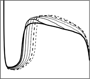
As expected, expressions (3.14) and (3.15) suggest that an accelerating jet causes thinning of the boundary layer and the film, whereas a decelerating jet causes them to thicken. Although our focus in this study will be on an accelerating jet from one steady state to another, it is helpful here to illustrate the nonlinear flow response for a sinusoidally pulsating jet. The response up to the transition point of  $\bar{\delta }(\bar{r} < {\bar{r}_0},\bar{t})$ and $\bar{h}(\bar{r} < {\bar{r}_0}(\bar{t}),\bar{t})$ is depicted in figure 2 for $W(\bar{t}) = 1 + {\textstyle{1 \over 2}}\ \textrm{sin}(({\rm \pi} /5)\bar{t})$. The radial and time dependence of $\bar{\delta }$ and $\bar{h}$ is illustrated by three-dimensional surface plots in figure 2(a,c), where the locus of the transition points is indicated by the black curve. The evolution of $\bar{\delta }$ and $\bar{h}$ at different radial positions is depicted in figure 2(b,d). We find that, even though the jet velocity profile is sinusoidal (symmetric peak and valley), the flow response is asymmetric. As reflected in figure 2(b,d), both $\bar{\delta }$ and $\bar{h}$ exhibit a narrowing in the peak region and a widening in the valley region.
Evolution of the boundary-layer thickness and film height for a pulsating jet of velocity  $W(\bar{t}) = 1 + {\textstyle{1 \over 2}}\,\textrm{sin}(({\rm \pi} /5)\bar{t})$. The evolution is plotted over two periods. A three-dimensional perspective is given in (a,c); the black curve in the surface plots represents the locus of the transition points demarking the end of the developing boundary-layer region at different times. The evolution of $\bar{\delta }$ and $\bar{h}$ in (b,d) are plotted against time at three different radial positions.

3.2. The transient fully developed viscous formulation
As mentioned previously, the potential flow in the radial direction ceases to exist in the fully developed viscous region, with the velocity at the free surface becoming dependent on the radial distance
 \begin{equation}u({r_0} < r < {r_J},z = h,t) = s(r,t).\end{equation}
In addition to the zero-shear-stress condition (2.3b), the pressure must also vanish at the free surface. By integrating (2.1c), for  ${r_0} \le r \le {r_J}$, with respect to z, subject to $p({r_0} \le r \le {r_J},z = h,t) = 0$, we obtain the expression of the hydrostatic pressure in this region as
 \begin{equation}p({r_0} \le r \le {r_J},z,t) = \frac{{h({r_0} \le r \le {r_J},t) - z}}{{F{r^2}}}.\end{equation}
We again assume a cubic velocity profile, but now subject to conditions (2.2a), (2.3b) and (3.16). In this case, the radial velocity profile is given in terms of the surface velocity  $s(r,t)$ as
 \begin{equation}u({r_0} < r < {r_J},z,t) = s(r,t)f(\eta ) = s(r,t)\left( {\tfrac{3}{2}\eta - \tfrac{1}{2}{\eta^3}} \right),\end{equation}
where  $\eta = z/h(r,t)$. Here, we observe that $f(\eta )$ is still given as in (3.7). Substituting (3.18) into the mass conservation equation (2.5), we obtain the following equation for the film thickness and surface velocity:
 \begin{equation}\frac{8}{5}{h_t} + s{h_r} + h{s_r} + \frac{{hs}}{r} = 0.\end{equation}
Clearly, unlike the steady state, the surface velocity is not readily expressible in terms of the film height; a second equation is needed, namely from momentum conservation. The momentum equation in the fully developed viscous region is still given by (2.1b).
Similar to (3.5), the integral form of the momentum equation reads
 \begin{equation}
\int_0^h {{u_t}\,\textrm{d}z} + \frac{1}{r}\frac{\partial}{\partial r}
\left({r\int_0^h {{u^2}\,\textrm{d}z}}\right)+s{h_t} ={-} \frac{1}{F{r^2}}h{h_r} - \frac{1}{Re}{u_z}(r,z = 0,t).\end{equation}
\begin{equation}
\int_0^h {{u_t}\,\textrm{d}z} + \frac{1}{r}\frac{\partial}{\partial r}
\left({r\int_0^h {{u^2}\,\textrm{d}z}}\right)+s{h_t} ={-} \frac{1}{F{r^2}}h{h_r} - \frac{1}{Re}{u_z}(r,z = 0,t).\end{equation}
However, upstream of the jump, the effect of gravity is weak, and the film depth and its variation are small. Therefore, the term  $- (Re/F{r^2})h{h_r}$ becomes negligible. Substituting (3.18) into (3.20), we obtain the second equation for the film thickness and surface velocity
 \begin{equation}
\frac{5}{8}h{s_t} +
\frac{5}{8}s{h_t} + \frac{{17}}{{35}}{s^2}{h_r} +
\frac{{17}}{{35}}\frac{{{s^2}h}}{r} +
\frac{{34}}{{35}}hs{s_r} + \frac{3}{{2Re}}\frac{s}{h} =
0.\end{equation}
\begin{equation}
\frac{5}{8}h{s_t} +
\frac{5}{8}s{h_t} + \frac{{17}}{{35}}{s^2}{h_r} +
\frac{{17}}{{35}}\frac{{{s^2}h}}{r} +
\frac{{34}}{{35}}hs{s_r} + \frac{3}{{2Re}}\frac{s}{h} =
0.\end{equation}
Using the rescaling (3.10a–c), (3.19) and (3.21) can be recast as
 \begin{gather}\frac{8}{5}{h_{\bar{t}}} + s{\bar{h}_{\bar{r}}} + \bar{h}{s_{\bar{r}}} + \frac{{\bar{h}s}}{{\bar{r}}} = 0,\end{gather}
 \begin{gather}\frac{5}{8}\bar{h}{s_{\bar{t}}} + \frac{5}{8}s{\bar{h}_{\bar{t}}} + \frac{{17}}{{35}}{s^2}{\bar{h}_{\bar{r}}} + \frac{{17}}{{35}}\frac{{{s^2}\bar{h}}}{{\bar{r}}} + \frac{{34}}{{35}}\bar{h}s{s_{\bar{r}}} + \frac{3}{2}\frac{s}{{\bar{h}}} = 0,\end{gather}
subject to the following boundary conditions:
 \begin{equation}\bar{h}(\bar{r} = {\bar{r}_0},\bar{t}) = {\bar{h}_0}(\bar{t}),\quad s(\bar{r} = {\bar{r}_0},\bar{t}) = W(\bar{t}).\end{equation}
Initial conditions are needed and are provided once a specific problem is examined. Equations (3.22a) and (3.22b) are solved using a backward implicit finite-difference discretisation in time of first-order accuracy, and integrating the resulting discretised equations using the Runge–Kutta fourth–fifth-order method (ode45 solver in MATLAB software). The absolute and relative tolerances were set to  ${10^{ - 12}}$. We note that discretising these equations in time instead of space is easier to implement numerically in this case since the spatial domain in this region changes with time as the transition point evolves. However, a spatial discretisation and time integration of the equations is still achievable upon introducing a spatial coordinate mapping. We tried both approaches and obtained full agreement.
3.3. The transient formulation across the jump
In this section, we consider the unsteady axisymmetric flow across the jump. As in the case of steady axisymmetric flow, we expect the flow through the hydraulic jump to incur a considerable loss of energy, which is usually difficult to determine. As such, the energy equation is not suitable for the analysis of the transient hydraulic jump (Crowe Reference Crowe2009). Alternatively, we apply the usual momentum balance approach across the jump, accounting for the surface tension effect due to the hoop stress (Bush & Aristoff Reference Bush and Aristoff2003). We consider a sharp jump assumption which is often adopted in the literature and yields satisfactory predictions for the jump radius (Watson Reference Watson1964; Bush & Aristoff Reference Bush and Aristoff2003; Dressaire et al. Reference Dressaire, Courbin, Crest and Stone2010; Prince et al. Reference Prince, Maynes and Crockett2012; Wang & Khayat Reference Wang and Khayat2018). This assumption is also justified on the basis that the length of the separation region around the upstream end of the jump is short for large Fr (see for example the discussion by Bowles & Smith Reference Bowles and Smith1992; Higuera Reference Higuera1994, Reference Higuera1997; Scheichl et al. Reference Scheichl, Bowles and Pasias2018).
By integrating equation (2.1c), for  $r \ge {r_J}$, with respect to z, subject to $p(r \ge {r_J},z = h,t) = 0$, we obtain the expression of the hydrostatic pressure in the jump and subcritical regions as
 \begin{equation}p(r \ge {r_J},z,t) = \frac{{h(r \ge {r_J},t) - z}}{{F{r^2}}}.\end{equation}
Consequently, similar to the case in the fully developed viscous region, the integral form of the momentum equation in the jump region is also given by (3.20). However, the term  $- (Re/F{r^2})h{h_r}$ is now not negligible since the film depth and its variation are greater downstream of the jump and across it than upstream. Across the jump, (3.20) is applied for a control volume of width $\mathrm{\Delta }r = r_J^ +{-} r_J^ -$ in the radial direction, yielding the following discretised form:
 \begin{equation}Re\,\Delta r\int_0^h {{u_t}\,\textrm{d}z} + Re\,\Delta \int_0^h {{u^2}\,\textrm{d}z} ={-} \frac{{Re}}{{2F{r^2}}}\Delta {h^2} - \Delta r{u_z}(r,z = 0,t).\end{equation}
Under the assumption of a sharp jump ( $\mathrm{\Delta }r \to 0$), and following Bush & Aristoff (Reference Bush and Aristoff2003), we include the radial force due to surface tension associated with the circular curvature of the jump. In this case, (3.24) becomes
 \begin{align}&\int_0^{{h_J}(t)} {{u^2}(r = r_J^ - ,z,t)\,\textrm{d}z} - \int_0^{{H_J}(t)} {{U^2}(r = r_J^ + ,z,t)\,\textrm{d}z}\notag\\ &\quad = \frac{{H_J^2(t) - h_J^2(t)}}{{2F{r^2}}} + \frac{1}{{We}}\frac{{{H_J}(t) - {h_J}(t)}}{{{r_J}(t)}},\end{align}
where U is the subcritical velocity profile. We note that  ${h_J}(t) \equiv h(r = r_J^ - ,t)$ and ${H_J}(t) \equiv h(r = r_J^ + ,t)$. The first two terms in (3.25) represent the force due to flow inertia, the third term represents the hydrostatic pressure force and the last term accounts for the radial force due to surface tension. In terms of the dimensionless groups, (3.25), as written, depends explicitly on Fr and We, but implicitly on Re. Incidentally, the rescaling (3.10a–c) that was used to eliminate the Reynolds number in the supercritical region does not apply to the subcritical region. For this reason, the Re value, as well as the values of Fr and We, will be specified when the jump location is reported.
We also observe that, in order to evaluate the second integral term in (3.25), an expression of the velocity profile in the subcritical region must be sought. Depending on the examined problems, different assumptions can be made downstream of the jump, which, in turn, yield different evaluations of the subcritical velocity and film thickness profiles. For instance, an obstacle placed at the edge of the disk might control the downstream liquid depth to a certain level without any significant radial variation (Watson Reference Watson1964; Bush & Aristoff Reference Bush and Aristoff2003), whereas the absence of this obstacle causes a significant variation of the downstream film height as the fluid flows freely over the edge of the disk (Duchesne, Lebon & Limat Reference Duchesne, Lebon and Limat2014). In the present study, the fluid is assumed to flow freely off the edge of the disk.
3.4. The transient subcritical lubrication flow
Following Duchesne et al. (Reference Duchesne, Lebon and Limat2014) for steady flow, we adopt a lubrication flow assumption downstream of the jump where the flow is slow and deep (see also Wang & Khayat Reference Wang and Khayat2018, Reference Wang and Khayat2019). Accordingly, the convective acceleration term is neglected in the momentum equation. Moreover, since we do not treat highly transient diffusive problems, the process time  ${t_p}$ is assumed to be much larger than both the local convective and diffusive times (Lang, Santhanam & Wu Reference Lang, Santhanam and Wu2017). In this case, ${t_p} \gg a/{V_0} \gg {a^2}/\nu $ or $Sr \gg 1 \gg Re$, where $Sr = {t_p}{V_0}/a$ is the Strouhal number. Therefore, both local and convective accelerations become negligible for the lubrication flow considered. Consequently, from the momentum equation, the hydrostatic pressure and the viscous effects balance to give
 \begin{equation}- \frac{{Re}}{{F{r^2}}}{H_r} + {U_{zz}} = 0.\end{equation}
Integrating (3.26) subject to (2.2a) and (2.3b), we obtain the subcritical velocity profile as
 \begin{equation}U(r > {r_J},z,t) = \frac{{Re}}{{F{r^2}}}{H_r}\left( {\frac{{{z^2}}}{2} - Hz} \right).\end{equation}
In order to determine the downstream film thickness, the mass conservation (2.5) is applied for  $r > {r_J}(t)$
 \begin{equation}\begin{array}{ccccc} & 2\int_0^{{r_0}(v)} {r{h_t}\,\textrm{d}r} + 2\int_{{r_0}(t)}^{r_J^ - (t)} {r{h_t}\,\textrm{d}r} + 2\int_{r_J^ - (t)}^{r_J^ + (t)} {r{H_t}\,\textrm{d}r} + 2\int_{r_J^ + (t)}^{r > r_J^ + (t)} {r{H_t}\,\textrm{d}r} \\ & \quad + 2r\int_0^{H(r,t)} {U(r,z,t)\,\textrm{d}z} = W(t). \end{array}\end{equation}
Evaluating (3.9a) at  $r = {r_0}(t)$, we obtain $\int_0^{{r_0}(t)} {r{h_t}\,\textrm{d}r} ={-} {\textstyle{5 \over 8}}W{r_0}{h_0} + W$. Next, by rewriting (3.19) as $r{h_t} ={-} {\textstyle{5 \over 8}}{(rsh)_r}$, we have $\int_{{r_0}(t)}^{r_J^ - (t)} {r{h_t}\,\textrm{d}r} ={-} {\textstyle{5 \over 8}}(r_J^ - {s_J}{h_J} - {r_0}W{h_0})$, where ${s_J}(t) \equiv s(r = r_J^ - ,t)$. As to the third integral term in (3.28), it becomes negligible in the limit $r_J^ - \to r_J^ + $ as long as the evolution of the film thickness remains finite across the jump width. Thus, in the limit of a sharp jump, (3.28) reduces to
 \begin{equation}\int_{{r_J}(t)}^{r > {r_J}(t)} {r{H_t}\,\textrm{d}r} + r\int_0^{H(r,t)} {U(r,z,t)\,\textrm{d}z} = \tfrac{5}{8}{r_J}{s_J}{h_J}.\end{equation}
By rescaling (3.29) using the appropriate scaling parameters, we find that the first term is of order O(1/Sr). Thereby, the condition  $Sr \gg 1$ established earlier causes the first integral term in (3.29) to vanish. In this case, (3.29) reduces to $r\int_0^{H(r,t)} {U(r,z,t)\,\textrm{d}z} = {\textstyle{5 \over 8}}{r_J}{s_J}{h_J}$. Recalling (3.27), the conservation of mass equation reduces to
 \begin{equation}{H_r} ={-} \frac{{15}}{8}\frac{{F{r^2}}}{{Re}}\frac{{{r_J}{s_J}{h_J}}}{{r{H^3}}}.\end{equation}
A boundary condition on the film thickness is needed to solve (3.30), which is specified by imposing the thickness at the edge of the disk,  ${H_\infty } = H(r = {r_\infty },t)$. Direct measurements by Duchesne et al. (Reference Duchesne, Lebon and Limat2014) of this edge thickness, performed at nearly 5 mm of the disk perimeter in their experiment, gave a nearly constant value of 1.5 mm with a weak power-law dependence on the flow rate not exceeding a few per cent. This constant thickness value was very close to the capillary length $\sqrt {\gamma /\rho g} $ of the fluid. This suggests that the edge thickness is established from the balance of forces between the hydrostatic pressure and the surface tension at the disk perimeter (Lubarda & Talke Reference Lubarda and Talke2011; Wang & Khayat Reference Wang and Khayat2018). This value is also consistent with the measurements of Dressaire et al. (Reference Dressaire, Courbin, Crest and Stone2010) for water. Therefore, we can assume here that the film thickness at the edge of the disk is essentially equal to the film thickness the liquid exhibits under static conditions. In a recent study, Wang & Khayat (Reference Wang and Khayat2018) showed that this assumption is accurate as it yielded a good agreement between theory and experiment for steady axisymmetric hydraulic jump. They also included a dynamic contribution based on energy minimisation at the disk edge. However, this contribution turned out to be negligible compared with the static contribution. In the present work, we follow Wang & Khayat (Reference Wang and Khayat2018) and assume that ${H_\infty } = (2/\sqrt {Bo} )\ \textrm{sin}({\theta _y}/2)$, where ${\theta _y}$ is the contact angle, and $Bo = We/F{r^2} = \rho {g_0}{a^2}/\gamma$ is the Bond number. We note that the edge thickness is assumed to remain independent of time (or flow rate) under transient conditions. This assumption will also turn out to be reasonable when we examine the thickness profiles from the numerical simulation to be discussed shortly.
Upon integrating (3.30) subject to  $H(r = {r_\infty },t) = {H_\infty }$, we obtain an analytical expression for the subcritical film thickness
 \begin{equation}H(r,t) = {\left( {H_\infty^4 + \frac{{15}}{2}\frac{{F{r^2}}}{{Re}}{r_J}{s_J}{h_J}\ \textrm{ln}\left( {\frac{{{r_\infty }}}{r}} \right)} \right)^{1/4}}.\end{equation}
By substituting the supercritical velocity profile (3.16) and the subcritical velocity profile (3.27) into (3.25), the momentum balance equation across the jump reduces to
 \begin{equation}\frac{{17}}{{35}}{h_J}s_J^2 - \frac{{15}}{{32}}\frac{{s_J^2h_J^2}}{{{H_J}}} - \frac{{H_J^2 - h_J^2}}{{2F{r^2}}} - \frac{1}{{We}}\frac{{{H_J} - {h_J}}}{{{r_J}}} = 0.\end{equation}
We note that, although the time does not appear explicitly in (3.32), it is implicit through the time dependence of  ${r_J}$, ${h_J}$, ${s_J}$ and ${H_J}$. We also note from (3.31) that ${H_J}(t) = H({r_J},t) = {(H_\infty ^4 + {\textstyle{{15} \over 2}}(F{r^2}/Re){r_J}{s_J}{h_J}\ \textrm{ln}({r_\infty }/{r_J}))^{1/4}}$, which is substituted in (3.32).
By solving numerically problem (3.22) subject to initial conditions, the film thickness  $h(r,t)$ and surface velocity $s(r,t)$ are obtained, and, subsequently, the jump location is determined at any time when (3.32) is satisfied. However, it should be noted that (3.32) is a cubic equation in ${H_J}$, and thereby, three different roots can be obtained numerically. Two roots are discarded as one corresponds to a negative ${H_J}$ and the other yields an ${H_J}$ very close to ${h_J}$ (not physically realistic). Approximately, this is confirmed by noting that the coefficients of the first two terms are very close, yielding ${H_J} \approx {h_J}$ as one of the three roots of (3.32). Consequently, the only viable root is approximately given by
 \begin{equation}{H_J} \approx{-} \left( {\frac{{{h_J}}}{{2F{r^2}}} + \frac{1}{{{r_J}We}}} \right) + \sqrt {\frac{{h_J^2}}{{4F{r^4}}} + \frac{1}{{r_J^2W{e^2}}} + \frac{{{h_J}}}{{{r_J}We\,F{r^2}}} + \frac{{34}}{{35}}\frac{{s_J^2{h_J}}}{{F{r^2}}}} .\end{equation}
Finally, by substituting (3.30) into (3.27) and evaluating (3.27) at z = H, we obtain the subcritical surface velocity as
 \begin{equation}S(r > {r_J}(t),t) = \frac{{15}}{{16}}\frac{{{r_J}{s_J}{h_J}}}{{rH}}.\end{equation}
4. Results and validation
The results in this section comprise a comparison with experiment for steady flow. We then consider the situation of a jet that undergoes a linear acceleration from one steady state to another at a constant rate. In this case, the jet velocity profile is given as
 \begin{equation}W(\bar{t}) = \left\{ {\begin{array}{*{20}{@{}ll}} {1,}&{\bar{t} \le 0}\\ {1 + A\bar{t},}&{0 \le \bar{t} \le {{\bar{t}}_c}}\\ {1 + A{{\bar{t}}_c},}&{\bar{t} \ge {{\bar{t}}_c}} \end{array}} \right.\end{equation}
where A is the dimensionless acceleration of the jet and  ${\bar{t}_c}$ is the acceleration period at the end of which the jet velocity becomes constant. Accordingly, our purpose is to study the transient response of the flow subject to this imposed jet velocity profile. Next, we examine the transient flow behaviour in the different regions of the domain for $A = 0.022$ and ${\bar{t}_c} = 50$. In this case, near impingement, the condition $\dot{W}/{W^2} \ll 182/121\bar{r}$, established earlier in § 3.1, is satisfied, and the flow is quasi-steady in the developing boundary-layer region.
4.1. Validation against experiment for steady flow
In order to validate the formulation, particularly justifying the assumptions of the cubic velocity profile in the supercritical region and the lubrication flow in the subcritical region, we first compare our predictions against experiment for the steady circular jump. In this case, we set  $W = 1$. Comparison between our predictions and the measurements of Duchesne et al. (Reference Duchesne, Lebon and Limat2014) is reported in figure 3 for the film thickness distribution in the super- and subcritical regions for silicon oil (20 cSt). The data are reproduced here in dimensionless form from their figure 2, corresponding to Re = 169, Fr = 16.88, We = 339 and a normalised disk radius ${\bar{r}_\infty } = 16.95$. The theoretical value of the thickness at the edge of the disk was fixed to ${\bar{H}_\infty } = 4.6$, corresponding to a contact angle ${\theta _Y} = {53^ \circ }$. Figure 3 shows that the theoretical predictions are generally in close agreement with the measurements of Duchesne et al. (Reference Duchesne, Lebon and Limat2014), slightly underestimating the measured thickness in the supercritical region. The location of the jump is predicted accurately whereas the jump height is slightly higher than experiment.
Comparison in terms of the free-surface profile between theoretical predictions and measurements of Duchesne et al. (Reference Duchesne, Lebon and Limat2014) for silicon oil (20 cSt). Results are plotted in dimensionless form for Re = 169, Fr = 16.88, We = 339 and  ${\bar{r}_\infty } = 16.95$.

4.2. The transient response of the flow in the developing boundary-layer region
The time interval  $\bar{t} \le 0$ corresponds to the initial steady state where $W = 1$. In this case, the initial steady-state profiles of the boundary-layer thickness and the film height are (Wang & Khayat Reference Wang and Khayat2018)
 \begin{equation}\bar{\delta }(\bar{r} < {\bar{r}_0},\bar{t} \le 0) = 2\sqrt {\frac{{70}}{{39}}\bar{r}} ,\quad \bar{h}(\bar{r} < {\bar{r}_0},\bar{t} \le 0) = \frac{1}{4}\left( {\frac{2}{{\bar{r}}} + \sqrt {\frac{{210}}{{13}}\bar{r}} } \right).\end{equation}
We note that (4.2a) and (4.2b) constitute the leading-order terms in (3.14) and (3.15), respectively, for  $W = 1$. Consequently, the initial conditions (3.12c) and (3.13c) are now given as
 \begin{equation}{Z_0}(\bar{r}) = \frac{{280}}{{39}}{\bar{r}^3},\quad {Y_0}(\bar{r}) = \frac{1}{4}\left( {2 + \sqrt {\frac{{210}}{{13}}} {{\bar{r}}^{3/2}}} \right).\end{equation}
Figure 4 illustrates the transient development of the boundary-layer thickness and the film height in the developing boundary-layer region at equal time intervals, subject to the jet velocity profile (4.1). Shown is the numerical solution for  $\bar{\delta }(\bar{r},\bar{t})$ and $\bar{h}(\bar{r},\bar{t})$, which closely agrees with their approximate counterparts established earlier in (3.14) and (3.15), to leading order. In this case, (3.9a) reduces essentially to the familiar steady-state form: $\bar{h}(\bar{r},\bar{t}) = {\textstyle{3 \over 8}}\bar{\delta }(\bar{r},\bar{t}) + 1/2\bar{r}$ (Wang & Khayat Reference Wang and Khayat2018). At $\bar{t} = 0$, W = 1, and the classical boundary-layer result is recovered (Watson Reference Watson1964; Schlichtling & Gersten Reference Schlichtling and Gersten2000). The profiles in figure 4 do not show a deviation from the classical parabolic character of the boundary-layer height, as the jet accelerates. We observe that since the boundary-layer height is small near the origin, the film height decays like $\bar{h}\sim 1/2\bar{r}$, regardless of the jet velocity value. This behaviour is also reflected by the $\bar{h}$ curves in figure 4, showing a narrow spread as time varies compared with $\bar{\delta }$. In particular, the $\bar{h}$ curves tend to saturate near impingement. Accelerating the jet tends to lower both the boundary-layer height and the film thickness with time. Therefore, the jet acceleration has a similar effect of thinning the boundary layer as with slip (Prince et al. Reference Prince, Maynes and Crockett2012; Khayat Reference Khayat2016), disk rotation (Wang & Khayat Reference Wang and Khayat2018) and gravity for high-viscosity liquids (Wang & Khayat Reference Wang and Khayat2019). Figure 4 also suggests that $\bar{\delta }(\bar{r},\bar{t})$ and $\bar{h}(\bar{r},\bar{t})$ do not exhibit a long-term transient behaviour after the acceleration period ends $(\bar{t} \ge {\bar{t}_c})$; that is, the flow reaches the steady state the moment the acceleration is halted. We shall see that this is not the case for the flow in the fully developed viscous region.
The transient behaviour of the developing boundary-layer region for a linearly accelerated jet. The rescaled boundary-layer height,  $\bar{\delta }(\bar{r},\bar{t})$, and film thickness, $\bar{h}(\bar{r},\bar{t})$, are plotted against the rescaled radial distance $\bar{r}$. The flow is examined subject to the jet velocity profile (4.1) for $A = 0.022$ and ${\bar{t}_c} = 50$. The curves $\bar{t} \ge 50$ represent the final steady-state profile for $\bar{\delta }$ and $\bar{h}$. The transition location coincides with the intersection of the two heights (at the cusps in the figure), indicated here by vertical lines. The blue curve represents the locus of the transition points demarking the end of the developing boundary-layer region at different times.

It is worth mentioning that the overall monotonic thinning behaviour of the film in this region due to the jet acceleration resembles the monotonic thinning behaviour of a fluid film lying on an accelerated stretching surface in the plane (Wang Reference Wang1990) and for axisymmetric flow (Usha & Sridharan Reference Usha and Sridharan1995). In those studies, a similarity solution was developed for the inversely linear unsteady (accelerating and decelerating) stretching. The actual film thickness evolution was found to be inversely proportional to the square root of the imposed stretching velocity. This behaviour is similar to the dependence of the film thickness evolution on the jet velocity at large radial positions depicted in figure 4.
We note that the behaviour of  $\bar{\delta }$ in figure 4 can also be deduced qualitatively from a balance argument from (3.4). By taking u to correspond to the free-surface value W $(u\sim W)$, the transient term $Re\,{u_t}$ cancels out with the radial pressure gradient term reflected by $Re\,\dot{W}$. Thus, the radial convective term and the viscous term must balance in (3.4): $Re\,u{u_r}\sim Re\,{W^2}/r$, leading to $\delta \sim \sqrt {r/W\,Re} $ or $\bar{\delta }\sim \sqrt {\bar{r}/W} $ which is in accordance with the leading-order term in (3.14).
The evolution of  $\bar{\delta }(\bar{r},\bar{t})$ and $\bar{h}(\bar{r},\bar{t})$ is illustrated in figure 5 at different radial positions in the developing boundary-layer region. In particular, the evolution of $\bar{\delta }$ at small time is compared against the developed approximate solution (A10) given in Appendix A, showing a good agreement for $\bar{t} < 1$ (see inset). In general, $\bar{h}$ decreases more slowly than $\bar{\delta }$; however, both $\bar{h}$ and $\bar{\delta }$ decrease at a lower rate with time as the jet accelerates. This behaviour can be inferred from ${\bar{h}_{\bar{t}}}\sim {\textstyle{3 \over 8}}{\bar{\delta }_{\bar{t}}}\sim{-} {\textstyle{3 \over 8}}{(1 + At)^{ - 3/2}}$ to leading order.
Evolution of the boundary-layer and film heights at different radial positions in the developing boundary-layer region for  $A = 0.022$ and ${\bar{t}_c} = 50$. The green dashed vertical line indicates the time ${\bar{t}_c} = 50$ at which the jet velocity as well as the boundary-layer and film heights all reach their final steady state. The inset shows a comparison for the evolution of the boundary-layer thickness at small time between the numerical solution (black curves) and approximate solution (A10) (blue curves).

Figure 6 depicts the evolution of the transition location  ${\bar{r}_0}(\bar{t})$ and corresponding film thickness ${\bar{h}_0}(\bar{t}) \equiv \bar{h}(\bar{r} = {\bar{r}_0})$. As the jet accelerates (inertia is enhanced), the transition point moves further downstream from impingement, and the corresponding film thickness decreases, but they both reach their final steady state at $\bar{t} = {\bar{t}_c}$. In fact, this behaviour can be deduced analytically by equating the leading-order terms in (3.14) and (3.15), yielding ${\bar{r}_0}(\bar{t}) \approx {({\textstyle{{78} \over {875}}}W)^{1/3}}$ or ${\bar{r}_0}(\bar{t}) \propto {W^{1/3}}$. Moreover, the relation $\bar{h}(\bar{r},\bar{t}) = {\textstyle{3 \over 8}}\bar{\delta }(\bar{r},\bar{t}) + 1/2\bar{r}$, established earlier, reduces to ${\bar{h}_0} = 4/5{\bar{r}_0}$ at the transition point, suggesting that ${\bar{h}_0}(\bar{t}) \propto {W^{ - 1/3}}$. For the initial steady state $(\bar{t} \le 0)$, since $W = 1$, we obtain ${\bar{r}_0} = {(78/875)^{1/3}} = 0.447$ and ${\bar{h}_0} = 1.791$, which are the values reflected in figure 6 at $\bar{t} = 0$. In comparison, Watson's steady transition point found using an exact solution of the boundary-layer equations is given as ${\bar{r}_0} = {(9\sqrt 3 c({\rm \pi} - c\sqrt 3 )/16{{\rm \pi} ^2})^{1/3}} = 0.463$, where $c = 1.402$ (Watson Reference Watson1964), which reflects a discrepancy of less than 3 %.
Evolution of the location and film thickness at the transition point between the developing boundary-layer and fully developed viscous regions for  $A = 0.022$ and ${\bar{t}_c} = 50$. The green dashed vertical line indicates the time ${\bar{t}_c} = 50$ at which W, as well as ${\bar{r}_0}$ and ${\bar{h}_0}$ all reach their final steady state.

The pressure distribution  $p(\bar{r},\bar{t})$ in the developing boundary-layer region is shown in figure 7. Here, we neglect the effect of gravity in the supercritical region. Therefore, expressions (3.3) and (3.17) reduce to $p(0 < r < {r_0},t) = ({r_0} - r)\dot{W}$ and $p({r_0} \le r \le {r_J},t) = 0$, respectively. Figure 7 indicates that the pressure in this region decreases linearly with the radial distance at different times for $\bar{t} \le {\bar{t}_c}$ and vanishes at the transition point. This linear decrease in the pressure follows a constant radial pressure gradient at all times because of the linear acceleration of the jet. The behaviour shown in figure 7 can be interpreted analytically by expressing the pressure, using (3.3), to obtain, to leading order: $p(\bar{r} < {\bar{r}_0},0 < \bar{t} < {\bar{t}_c}) = A({\bar{r}_0} - \bar{r}) \approx A[{({\textstyle{{78} \over {875}}}(1 + A\bar{t}))^{1/3}} - \bar{r}]$. As depicted in the inset of figure 7, for a given radial position, the beginning and the end of the acceleration period are accompanied by a sudden jump and a sudden drop in the pressure, respectively. However, during the acceleration period, the pressure increases nonlinearly with time. This behaviour resembles the one reported by Chang & Maxey (Reference Chang and Maxey1995) for the case of a linearly accelerated flow over a sphere, from one steady state to another (see their figure 6). They attributed the sudden changes in pressure to the added-mass effects, i.e. inertial effects added to the system because of the acceleration, which is the same driving mechanism of the transient response in the present problem.
The transient response of the pressure in the developing boundary-layer region for a linearly accelerated jet ( $A = 0.022$ and ${\bar{t}_c} = 50$). The curve $\bar{t} > 50$ indicates that $p = 0$ is the final steady state. The blue curve represents the locus of the transition points. The inset depicts the evolution of the pressure at different radial positions showing sudden changes at the beginning and at the end of the acceleration period.

4.3. The transient response of the flow in the fully developed viscous region
We now examine the flow response in the fully developed viscous region subject to the jet velocity profile (4.1). The initial steady-state profiles of the film thickness and the surface velocity are recalled as (Wang & Khayat Reference Wang and Khayat2018)
 \begin{gather}\bar{h}({\bar{r}_0} < \bar{r} < {\bar{r}_J},\bar{t} \le 0) = \frac{{175}}{{136}}{\bar{r}^2} + \frac{{233}}{{340\bar{r}}} = \frac{{175}}{{136\bar{r}}}({\bar{r}^3} - \bar{r}_0^3) + 2\frac{{{{\bar{r}}_0}}}{{\bar{r}}}\sqrt {\frac{{70}}{{39}}{{\bar{r}}_0}}, \end{gather}
 \begin{gather}s({\bar{r}_0} < \bar{r} < {\bar{r}_J},\bar{t} \le 0) = \frac{4}{{5\bar{h}\bar{r}}}.\end{gather}
We note that (4.4a) and (4.4b) are in close agreement with Watson's expressions, reproduced here in dimensionless forms as:  $\bar{h} \approx 1.28{\bar{r}^2} + 0.69/\bar{r}$ and $s \approx 0.81/\bar{h}\bar{r}$ (Watson Reference Watson1964), respectively.
The time-dependent boundary-layer height and supercritical film thickness are plotted against the radial distance at equal time intervals as shown in figure 8. We recall that the transition point moves downstream with time, as the jet accelerates. At any time, the film thickness exhibits a strong minimum followed by an increase with the radial distance. In the limit  $\bar{t} = 0$, (4.4a) indicates that the height increases like $\bar{h} \propto {\bar{r}^2}$ at large distance. For a faster jet, the film acquires additional radial momentum, with a reduced viscous effect. Therefore, it is apparent from figure 8 that, as the jet accelerates, the minimum film thickness weakens, accompanied by an overall thinning of the boundary layer and film. We observe that, close to the transition point, the film thickness in the fully developed viscous region decays at a slower rate at a later time than initially, a behaviour similar to that predicted in the boundary-layer region (see figure 5). Figure 8 indicates that the location of the minimum height moves downstream as the effect of viscosity gradually diminishes with time relative to inertia. The last point along the $\bar{h}$ curves marks the end of the fully developed viscous region at different times, coinciding with the jump occurrence.
Transient response of the developing boundary-layer height and film thickness in the supercritical region for a linearly accelerated jet ( $A = 0.022$ and ${\bar{t}_c} = 50$). The red curve represents the locus of the jump points (also indicated by the vertical lines) demarking the end of the fully developed viscous region at different times. The cyan curve represents the quasi-steady profile of the film thickness in the fully developed viscous region at $\bar{t} = 10$. Also indicated in vertical lines on the left are the transition point locations at different times. The curve $\bar{t} > 50$ represents the final steady-state profile of $\bar{\delta }$ and $\bar{h}$. The jump is determined for $Re = 100$, $Fr = 10$, $We = 120$, ${\bar{H}_\infty } = R{e^{1/3}}{H_\infty } = 5.1$ and ${\bar{r}_\infty } = R{e^{ - 1/3}}{r_\infty } = 5.38$.

We find that, far from the transition point, the actual instantaneous film thickness in the fully developed viscous region deviates from the quasi-steady state, and so does the jump location. We illustrate this deviation by adding the quasi-steady profile (in cyan) for  $\bar{t} = 10$ in figure 8. We also observe from the figure that the film thickness continues to decrease after the acceleration has ceased at $\bar{t} = {\bar{t}_c} = 50$. Thus, unlike the developing boundary-layer region, the film thickness in the fully developed viscous region exhibits a long-term transient behaviour, which is particularly evident at large $\bar{r}$; the thickness profile reaches its final steady state at a time $\bar{t} > {\bar{t}_c}$. This suggests that, despite the end of the acceleration period, inertial effects still induce a transient change in the flow, which is attributed to the intrinsic nonlinearities present in (3.22a) and (3.22b).
Figure 9 shows the evolution of the film thickness  $\bar{h}(\bar{r},\bar{t})$ in the fully developed viscous region at different radial positions. The quasi-steady states are also plotted (cyan curves) for comparison. It is shown that, initially, the actual instantaneous film thickness accumulates and deviates from the quasi-steady state given the significance of viscous effects (Telionis Reference Telionis1981), exhibiting a weak maximum when inertia becomes as important as viscous effects. The thickness then decays with time as inertia becomes dominant, and behaves closer to the quasi-steady state as reflected by the narrowing of the gap between the black and cyan curves in figure 9. The purple curve, representing the locus of the maximum film thickness at different radial positions, shows an earlier occurrence of this maximum at smaller $\bar{r}$. This transient behaviour of the film thickness (early-stage maximum before decaying with time) is similar to the one observed in the case of a laminar film suddenly accelerated by gravity and falling inside a vertical circular tube as studied experimentally by Zhong et al. (Reference Zhong, He and Longtin2020) (see their figure 9). Furthermore, we observe that the film thickness reaches its final steady state at $\bar{t} \approx {\bar{t}_c}$ for small $\bar{r}$, and at $\bar{t} > {\bar{t}_c}$ for large $\bar{r}$, as reflected by the green solid curves in figure 9 and the inset, respectively, suggesting that the long-term transient response in the film thickness is particularly evident at large $\bar{r}$.
Evolution of the film thickness in the fully developed viscous region at different radial positions for  $A = 0.022$ and ${\bar{t}_c} = 50$. The purple curve represents the locus of the maximum film thickness, the cyan curves represent the quasi-steady film thickness profiles and the green solid curve represents the locus of the final steady state. The inset depicts the evolution of $\bar{h}$ at large radial positions for $\bar{t} > 40$, showing that the final steady state is reached at $\bar{t} > {\bar{t}_c}$.

As discussed earlier (figure 8), the parabolic profile of the film thickness in the fully developed viscous region exhibits a minimum at any time. The time variation of this minimum film thickness, denoted by  ${\bar{h}_{min}}(\bar{t})$, and its corresponding radial position, denoted by ${\bar{r}_{min}}(\bar{t})$, are plotted in figure 10. At the early stage of the flow, as viscous effects are important, ${\bar{h}_{min}}$ exhibits a weak maximum, while ${\bar{r}_{min}}$ exhibits a weak minimum. As viscous effects gradually diminish with time relative to inertia, the minimum film height weakens and occurs further downstream.
Evolution of the minimum film thickness and its corresponding radial position in the fully developed viscous region for  $A = 0.022$ and ${\bar{t}_c} = 50$.

The transient behaviour of the supercritical free-surface velocity is depicted in figure 11. As seen in figure 11(a), at any time, the surface velocity remains equal to the jet velocity in the developing boundary-layer region, as reflected by the horizontal lines, before it decreases monotonically with distance downstream of the transition location in the fully developed viscous region. At  $\bar{t} = 0$, the monotonic decrease of s with respect to $\bar{r}$ is recalled from the initial steady-state solution by substituting (4.4a) into (4.4b)
 \begin{equation}s({\bar{r}_0} < \bar{r} < {\bar{r}_J},\bar{t} \le 0) = \frac{4}{5}{\left( {\frac{{175}}{{136}}({{{\bar{r}}^3} - \bar{r}_0^3} )+ 2{{\bar{r}}_0}\sqrt {\frac{{70}}{{39}}{{\bar{r}}_0}} } \right)^{ - 1}}.\end{equation}
In this case (at  $\bar{t} = 0$), s decreases like ${\bar{r}^{ - 3}}$ at large distance, and we can clearly observe from figure 11(a) a similar behaviour at subsequent times. We can also see that the jet acceleration increases the surface velocity of the flow with time (see figure 11b), but diminishes the rate at which it decreases with radial distance (see figure 11a), which is similar to the effect of slip (Prince et al. Reference Prince, Maynes and Crockett2012; Khayat Reference Khayat2016) and disk rotation (Wang & Khayat Reference Wang and Khayat2018). We observe that s = W at $\bar{r} = 0.3$ in figure 11(b), since this radial position belongs to the developing boundary-layer region at all times. Figure 11(b) and the inset in figure 9 show that, similar to the film thickness, the long-term transient behaviour of the surface velocity in the fully developed viscous region is particularly evident at large radial positions. This is depicted by the green solid curve representing the locus of the final steady state (see for example the time at which $\bar{h}$ and s reach their final steady state for $\bar{r} = 1.7$ compared with $\bar{r} = 0.9$).
Transient behaviour of the supercritical surface velocity for  $A = 0.022$ and ${\bar{t}_c} = 50$. The radial dependence of s is plotted at equal time intervals (a), and the evolution of s is plotted at different radial positions in the supercritical region (b). The blue curve represents the locus of the transition points whereas the red curve represents the locus of the jump points. The green solid curve represents the locus of the final steady state reached by s at different $\bar{r}$. The jump is determined for $Re = 100$, $Fr = 10$, $We = 120$, ${\bar{H}_\infty } = 5.1$ and ${\bar{r}_\infty } = 5.38$.

In figure 12, we present a three-dimensional surface plot to illustrate in detail the transient behaviour of the thin film in the fully developed viscous region. We show the evolution of both the film thickness as depicted by the height of the surface (z-axis), and surface velocity as described by the colour map. It is shown from the colour map that, upon accelerating the jet, the surface velocity at the transition location increases with time, which is also reflected by the blue curve in figure 11. However, the surface velocity does not change much at the hydraulic jump location, which is also reflected by the red curve in figure 11. Moreover, the projected curves in figure 12 indicate that the relative change between the final and initial steady states is larger for  ${\bar{r}_J}(\bar{t})$ and ${\bar{h}_J}(\bar{t})$ than for ${\bar{r}_0}(\bar{t})$ and ${\bar{h}_0}(\bar{t})$.
Surface plot showing the evolution of the film thickness and surface velocity contours in the fully developed viscous region for  $A = 0.022$ and ${\bar{t}_c} = 50$. The height of the surface reflects the film thickness while the colour map reflects the values of the surface velocity. The jump is determined for $Re = 100$, $Fr = 10$, $We = 120$, ${\bar{H}_\infty } = 5.1$ and ${\bar{r}_\infty } = 5.38$.

The wall shear stress at the disk is expressed as
 \begin{gather}{\bar{\tau }_w}(\bar{r} < {\bar{r}_0},\bar{t}) = \frac{3}{2}\frac{W}{{\bar{\delta }}},\end{gather}
 \begin{gather}{\bar{\tau }_w}({\bar{r}_0} < \bar{r} < {\bar{r}_J},\bar{t}) = \frac{3}{2}\frac{s}{{\bar{h}}}.\end{gather}
Always for the same jet velocity profile (4.1), figure 13 illustrates the transient behaviour of the wall shear stress. As seen in figure 13(a), at any time, the stress decays very rapidly with the radial distance in the developing boundary-layer region, which can be explained by referring to the leading-order solution in (3.14). In this case, (4.6a) reduces to
 \begin{equation}{\bar{\tau }_w}(\bar{r} < {\bar{r}_0},\bar{t}) \approx \sqrt {\frac{{39}}{{280}}\frac{{{W^3}}}{{\bar{r}}}} .\end{equation}
Equation (4.7) also suggests that, for a given radial position in the developing boundary-layer region,  ${\bar{\tau }_w}\sim {W^{3\; /2}}$, which resembles the dependence of the wall shear stress on the stretching velocity for a fluid film lying on an unsteady stretching surface (Wang Reference Wang1990; Usha & Sridharan Reference Usha and Sridharan1995). After its rapid drop in the developing boundary-layer region, ${\bar{\tau }_w}$ exhibits a maximum in the fully developed viscous region before decaying monotonically with the radial distance as in figure 13(a). For $\bar{t} = 0$, the monotonic decrease of ${\bar{\tau }_w}$ with respect to $\bar{r}$ is recalled from the initial steady-state solution by substituting (4.4a) and (4.4b) into (4.6b) to obtain
 \begin{equation}{\bar{\tau }_w}({\bar{r}_0} < \bar{r} < {\bar{r}_J},\bar{t} \le 0) = \frac{6}{5}\bar{r}{\left( {\frac{{175}}{{136}}({{\bar{r}}^3} - \bar{r}_0^3) + 2{{\bar{r}}_0}\sqrt {\frac{{70}}{{39}}{{\bar{r}}_0}} } \right)^{ - 2}}.\end{equation}
In this case (at  $\bar{t} = 0$), at large radial distance, the wall shear stress decays like ${\bar{r}^{ - 5}}$, and a similar behaviour is observed in figure 13(a) at subsequent times. Moreover, the rate at which the wall shear stress decays with radial distance increases as the jet accelerates. We observe that, since accelerating the jet causes a higher velocity gradient near the wall, we obtain a monotonic increase with time in the wall shear stress at any radial position in the supercritical region as depicted in figure 13(b). This can easily be explained by referring to (4.5a) and (4.5b), knowing that W and s increase with time, whereas $\bar{\delta }$ and $\bar{h}$ decrease overall. Figure 13(b) also shows a long-term transient response in ${\bar{\tau }_w}$ at large $\bar{r}$.
Transient behaviour of the supercritical wall shear stress for  $A = 0.022$ and ${\bar{t}_c} = 50$. The radial dependence of ${\bar{\tau }_w}$ is plotted at equal time intervals (a), and the evolution of ${\bar{\tau }_w}$ is plotted at different radial positions in the supercritical region (b). The blue curve represents the locus of the transition points whereas the red curve represents the locus of the jump points. The green solid curve represents the locus of the final steady state reached by ${\bar{\tau }_w}$ at different $\bar{r}$. The jump is determined for $Re = 100$, $Fr = 10$, $We = 120$, ${\bar{H}_\infty } = 5.1$ and ${\bar{r}_\infty } = 5.38$.

Finally, a monotonic increase with time in the wall shear stress was also reported by Seddighi et al. (Reference Seddighi, He, Vardy and Orlandi2014) for a linearly accelerating channel flow starting from an initially statistically steady turbulent flow (see their figure 3b). However, the friction coefficient, which was introduced as the actual wall shear stress normalised relative to the instantaneous bulk velocity instead of the average velocity, showed a non-monotonic evolution (see their figure 3c). Following Seddighi et al. (Reference Seddighi, He, Vardy and Orlandi2014), we introduce the friction coefficient at the disk in the supercritical region as  ${C_f} = 2R{e^{ - 2/3}}{\bar{\tau }_w}/{W^2}$ where ${C_f}$ is the actual wall shear stress normalised by ${\textstyle{1 \over 2}}\rho {V^2}(t)$, and $V(t)$ is the dimensional instantaneous jet velocity, with $V(t = 0) = {V_0}$. In this case, the friction coefficient in the developing boundary-layer and fully developed viscous regions can be expressed as
 \begin{gather}{C_f}(\bar{r} < {\bar{r}_0},\bar{t}) = \frac{{3R{e^{ - 2/3}}}}{{W\bar{\delta }}},\end{gather}
 \begin{gather}{C_f}({\bar{r}_0} < \bar{r} < {\bar{r}_J},\bar{t}) = \frac{{3R{e^{ - 2/3}}s}}{{{W^2}\bar{h}}},\end{gather}
respectively. Figure 14 shows the transient behaviour of the supercritical friction coefficient. We observe from figure 14(a) that, at any time, the radial dependence of the friction coefficient follows the radial dependence of the wall shear stress shown earlier in figure 13(a). Interestingly, in the fully developed viscous region, in contrast to the monotonic response of the shear stress (see figure 13b for  $\bar{r} > 0.5$), ${C_f}$ exhibits a non-monotonic transient behaviour as depicted in figure 14(b). This occurs further downstream in the fully developed viscous region at the radial positions that show a weak maximum in the film thickness, namely at $\bar{r} = 0.9$, 1 and 1.1 (see also figure 9). We observe that, at these radial positions, ${C_f}$ decreases initially with the increase in the film thickness, exhibiting an early weak minimum coinciding with the weak maximum in the film thickness. As the flow continues to accelerate, the friction coefficient increases as a result of the low flow momentum that is pushed inside of the boundary layer against the wall, simultaneously reducing the overall film thickness. This non-monotonic behaviour of the friction coefficient shown in figure 14(b) is parallel to the one observed by Seddighi et al. (Reference Seddighi, He, Vardy and Orlandi2014) as reported in their figure 3(c). In their case, the friction coefficient behaves oppositely to the boundary-layer thickness, whereas in our case, the friction coefficient behaves oppositely to the film thickness.
Transient behaviour of the friction coefficient in the supercritical region for  $A = 0.022$ and ${\bar{t}_c} = 50$. The radial dependence of ${C_f}$ is plotted at equal time intervals (a), and the evolution of ${C_f}$ is plotted at different radial positions in the fully developed viscous region (b). The blue curve represents the locus of the transition points whereas the red curve represents the locus of the jump points. The green solid curve represents the locus of the final steady state reached by ${C_f}$ at different $\bar{r}$. The jump is determined for $Re = 100$, $Fr = 10$, $We = 120$, ${\bar{H}_\infty } = 5.1$ and ${\bar{r}_\infty } = 5.38$.

4.4. Evolution of the hydraulic jump radius and comparison with the numerical simulation
A numerical simulation of a transient jet impinging over a stationary horizontal disk was carried out using the Ansys Fluent software. Silicone oil was considered with the following physical properties:  $\rho = 950\;\textrm{kg}\;{\textrm{m}^{ - 3}}$, $\mu = 19\;\textrm{mPa}\;\textrm{s}$ and $\gamma = 20\;\textrm{dyn}\;\textrm{c}{\textrm{m}^{ - 1}}$. The nozzle radius was taken as $a = 1.6\;\textrm{mm}$ and the initial jet flow rate was $Q = 10\;\textrm{ml}\;{\textrm{s}^{ - 1}}$. These parameters correspond to the steady-state experiment carried out by Duchesne et al. (Reference Duchesne, Lebon and Limat2014) for a plate radius of 150 mm and a disk-to-nozzle distance of 16 mm, except that their operating flow rate was $Q = 17\;\textrm{ml}\;{\textrm{s}^{ - 1}}$. In addition, we have shortened the radius of the disk to 40 mm and the disk-to-nozzle distance to 8 mm to lower the computational cost. In terms of the dimensionless parameters, this corresponds to $Re = 100$, $Fr = 10$, $We = 120$ and ${\bar{r}_\infty } = 5.38$.
The numerical model was previously validated against the measurements of Duchesne et al. (Reference Duchesne, Lebon and Limat2014) for steady state (Wang & Khayat Reference Wang and Khayat2021). In order to study the linearly accelerated jet, the jet velocity profile (4.1) was imposed in the present numerical simulation, where A = 0.022 and  ${\bar{t}_c} = 50$. The flow was allowed to fall freely over the edge of the disk in the absence of any obstacle.
As the flow is assumed to be axisymmetric, polygonal jumps (Rojas & Tirapegui Reference Rojas and Tirapegui2015) are not considered. In this case, we solve the axisymmetric version of the full Navier–Stokes equations in cylindrical coordinates (see Wang & Khayat Reference Wang and Khayat2021 for details), with the gas–liquid interface (i.e. the free surface) tracked by an extra scalar field using the volume of fluid (VOF) approach (Hirt & Nichols Reference Hirt and Nichols1981). The physical and computational domains are shown in figure 15 with the dimensions shown along the corresponding sides of the domain. The simulation is carried out using a finite volume solver (Ansys Fluent), with the primary variables located at the centroid of the mesh cells. The fluxes at the cell surface are calculated based on the interpolated values of the cell centroid. With the VOF method, the free surface is tracked by a transport equation that governs the volume fraction of the liquid phase, namely
 \begin{equation}\frac{\partial }{{\partial t}}{\alpha _l} + {\boldsymbol{v}_l}\boldsymbol{\cdot }\boldsymbol{\nabla }{\alpha _l} = 0,\end{equation}
with  ${\alpha _l}$ being the volume fraction of the liquid, and therefore ${\alpha _g} = 1 - {\alpha _l}$ being the gas fraction. Here, ${\boldsymbol{v}_l}$ is the velocity vector of the liquid. With this approach, only a single set of transport equations is solved. The values of variables and fluid properties at the centroid of each cell represent the volume-weighted averages based on the fraction of the two phases.
The three-dimensional physical domain and the two-dimensional axisymmetric computational domain of the numerically simulated flow.

The standard Semi-Implicit Method for Pressure Linked Equations-Consistent (SIMPLEC) scheme (Van Doormaal & Raithby Reference Van Doormaal and Raithby1984) is selected for pressure correction. For spatial discretisation, we adopt the second-order Quadratic Upstream Interpolation for Convective Kinematics (QUICK) scheme (Leonard & Mokhtari Reference Leonard and Mokhtari1990), which uses two upstream and one downstream value of the neighbouring cell centroid to interpolate the face values of the control volume for flux calculation. A second-order implicit time marching scheme is selected for the best stability. Finally, the volume fraction (4.10) is discretised by a second-order compressive scheme such that the face value of the volume fraction is given by  ${\phi _f} = {\phi _d} + 2\boldsymbol{\nabla }{\phi _d}\boldsymbol{\cdot }\boldsymbol{S}$, where ${\phi _f}$ is the volume fraction at the cell face between the donor (upstream) and acceptor (downstream) cell, ${\phi _d}$ is the volume fraction of the donor cell and $\boldsymbol{S}$ is the displacement vector from the donor cell centroid to the centroid of the cell face. Surface tension is considered using the continuum surface force model (Brackbill, Kothe & Zemach Reference Brackbill, Kothe and Zemach1992). The detailed reasons of these numerical choices can be found in the work of Wang & Khayat (Reference Wang and Khayat2021).
The pressure is set to atmospheric everywhere in the domain and the velocity is set to be zero initially. The domain is at first fully occupied by air, the silicon oil at a uniform velocity of flow rate Q = 10 ml s−1 is injected into the domain through the inlet of radius a = 1.6 mm until the first steady state is reached when a stable hydraulic jump has been formed. Then the flow rate starts to vary according to Q = 10 + 37.3t ml s−1. The impingement surface of radius R = 40 mm is at a distance D = 8 mm away from the inlet. The boundary conditions are also displayed in the computational domain. The pressure is set to be atmospheric at the right side of the computational domain (cf. figure 15). A sidewall near the trailing edge of the disk is constructed so that the flow can turn and flow off the domain under the action of gravity. We note that the upper boundary of the domain is set to a no-slip condition instead of atmospheric pressure as it turns out that overregulating the pressure sometimes drives the flow to an unrealistic state before reaching a steady state. The solution converges better when using a no-slip condition which allows the pressure to freely adjust itself according to the momentum evolution. Practically, this should not affect the solution much since the viscosity of the gas phase is usually negligible compared with that of the liquid, and the configuration is laminar. In addition, we refer to the satisfactory numerically simulated results obtained by Askarizadeh et al. (Reference Askarizadeh, Ahmadikia, Ehrenpreis, Kneer, Pishevar and Rohlfs2020) and Wang & Khayat (Reference Wang and Khayat2021), who also used a similar numerical configuration.
The convergence test is carried out at the steady state. Three sets of uniform grid sizes (the side length of the control volume) are tested, namely 0.32, 0.16 and 0.08 mm, treated as coarse, medium and fine meshes, respectively. It is found that the relative error in the jump location is well below 1 % between the medium and the fine mesh. In this case, the medium mesh size is sufficient and thus adopted in the transient numerical computation. For more details on the numerical convergence test, the reader is referred to the work of Wang & Khayat (Reference Wang and Khayat2021).
The evolution of the simulated flow in the (r, z) plane is depicted in figure 16 in terms of the volume fraction of the fluid at equal time intervals. As the jet accelerates, the location of the jump moves forward and the maximum film height increases.
Evolution of the simulated flow for  $A = 0.022$, ${\bar{t}_c} = 50$, $Re = 100$, $Fr = 10$, $We = 120$ and ${\bar{r}_\infty } = 5.38$. The volume fraction is presented for liquid (in red) and surrounding air (in blue), corresponding to ${\alpha _l} = 1$ and ${\alpha _g} = 0$, respectively. The liquid and gas phases are separated by the free surface ( $0 < \alpha < 1$).

The comparison of the free-surface height at equal time intervals between the theory and numerical simulation is shown in figure 17. Best comparison was achieved upon taking  ${\bar{H}_\infty } = 5.1$. This corresponds to an edge film thickness equal to 1.76 mm, which is close to the capillary length of the considered fluid (1.46 mm). It is shown that the theory predicts well the free-surface evolution of the fluid, except the gradual transition in the hydraulic jump region, due to the sharp jump assumption, as well as the turn-around region at the edge. These issues will be touched on later in § 5.
Comparison between theory (black solid curves) and numerical simulation (red circles). The free-surface height is shown at equal time intervals for  $A = 0.022$, ${\bar{t}_c} = 50$, $Re = 100$, $Fr = 10$, $We = 120$, ${\bar{H}_\infty } = 5.1$ and ${\bar{r}_\infty } = 5.38$.

We next quantify the comparison between the theory and numerical simulation in terms of the jump radius, the upstream and downstream jump heights, as depicted in figure 18, which show good agreement. As is apparent, even though the jet velocity increases linearly with time, the responses in  ${\bar{r}_J}$, ${\bar{h}_J}$ and ${\bar{H}_J}$ are predominantly linear only at later times. We note that the jump position deduced from the numerical simulation corresponds to the maximum radial gradient in the film thickness, and the downstream jump height corresponds to the numerical maximum film thickness. Due to our sharp jump assumption, the downstream jump height predicted theoretically cannot be directly compared against the one from the numerical simulation. However, the good agreement shown in figure 18 in terms of ${\bar{H}_J}$ was obtained upon reducing all the predicted values at all times by 11 % as a correction made to compensate for the sharp jump assumption.
Comparison between theory (lines) and numerical simulation (points). The evolution of the jump radius  ${\bar{r}_J}$, the upstream jump height ${\bar{h}_J}$ and the downstream jump height ${\bar{H}_J}$ are shown for a linearly accelerated jet for $A = 0.022$, ${\bar{t}_c} = 50$, $Re = 100$, $Fr = 10$, $We = 120$, ${\bar{H}_\infty } = 5.1$ and ${\bar{r}_\infty } = 5.38$.

Combining the simulated free-surface height at equal time intervals in one plot, as shown in figure 19, reveals an interesting transient dynamics, which is not necessarily captured by the thin-film theory. The figure indicates that the film height tends to exhibit an overshoot in the form of a localised maximum that diffuses with time. We also notice that, although the downstream film thickness increases with time, it always converges to the initial steady-state profile at a certain radial position that increases with time. In other words, the influence of inertia, as a result of the jet acceleration, on the downstream film height is not felt until later times. Moreover, we observe that the film thickness at the edge does not vary with time, as the film seems to be pinned there, making our earlier assumption of a time-independent  ${H_\infty }$ in our theory plausible. The overall increase in the downstream height is obviously accompanied by a rise in the pressure force, which acts on the jump to slow it down. However, the jump continues to move outward, reflecting the dominance of inertia over the pressure force as the jet accelerates.
The film profiles based on the numerical simulation at equal time intervals for  $A = 0.022$, ${\bar{t}_c} = 50$, $Re = 100$, $Fr = 10$, $We = 120$ and ${\bar{r}_\infty } = 5.38$.

The transient behaviour of the subcritical film thickness and surface velocity, predicted from (3.31) and (3.34), is shown in figure 20. Figure 20(a,c) shows the radial dependence of  $\bar{H}$ and S at equal time intervals, whereas figure 20(b,d) shows the evolution of $\bar{H}$ and S at different radial positions. We observe from figures 20(a) and 20(c) that, at any time, $\bar{H}$ and S decrease with the radial distance since the flow becomes slower near the edge. While $\bar{H}$ decreases monotonically with $\bar{r}$ similar to the case for steady flow, S exhibits a minimum close to the edge, which is not usually predicted or observed for steady flow. While $\bar{H}$ reaches the same constant level, S continues to grow with time, which is reflected in the curve corresponding to ${r_\infty }$ in figure 20(d). We observe from figures 20(b) and 20(d) that, for a given radial position, $\bar{H}$ and S increase with time during the acceleration period and overshoot their final steady states. The overshoot occurs at $\bar{t} \approx {\bar{t}_c}$ when the acceleration is halted. We recall from (3.23) that the pressure, downstream of the jump, is related to the film height, and therefore, the evolution of $\bar{H}$ in figure 20(b) reflects the evolution of the pressure. Consequently, figure 20(b) suggests that, similar to the transient behaviour of the pressure in the developing boundary-layer region (see figure 7), the pressure downstream of the jump also increases with time. However, no sudden changes occur before or after the acceleration period since the film height evolves smoothly with time. We also note that the pressure decreases with the radial distance in both the supercritical and subcritical regions. Finally, figure 20(b,c) shows that $\bar{H}$ and S reach their final steady state at $\bar{t} > {\bar{t}_c}$, suggesting that the long-term transient behaviour is not restricted to the supercritical region.
Transient behaviour of the subcritical film thickness and surface velocity for  $A = 0.022$ and ${\bar{t}_c} = 50$. The profiles of $\bar{H}$ and S are plotted against the radial distance at equal time intervals (a,c), and against time at different radial positions (b,d). The curves $\bar{t} > 50$ in (a,c) correspond to the final steady-state profiles. The red curve represents the locus of the jump points whereas the green solid curve represents the locus of the final steady state reached by $\bar{H}$ and S at different $\bar{r}$. The jump is determined for $Re = 100$, $Fr = 10$, $We = 120$, ${\bar{H}_\infty } = 5.1$ and ${\bar{r}_\infty } = 5.38$.

We now explore the effect of gravity, which is found to have a significant influence on the transient response of the jump. Therefore, we consider varying Fr while keeping Re and We fixed. The base case corresponds to the values taken in the comparison with the numerical simulation earlier, namely  $Re = 100$, $Fr = 10$ and $We = 120$. We also take ${\bar{H}_\infty } = 5.1$ and ${\bar{r}_\infty } = 5.38$. The influence of Fr on the transient response of the jump radius ${\bar{r}_J}(\bar{t})$, the upstream jump height ${\bar{h}_J}(\bar{t})$ and surface velocity ${s_J}(\bar{t})$, as well the downstream jump height ${\bar{H}_J}(\bar{t})$, is illustrated in figure 21. We also include the final steady state as the green solid curve. As expected, the jump radius increases with time as the jet is accelerated. For any Fr, ${\bar{r}_J}$ increases monotonically before reaching its final steady state (figure 21a). Similarly, the upstream and downstream jump heights also increase with time, but they overshoot their final steady-state level (see figure 21b,d) at a time close to $\bar{t} = {\bar{t}_c}$ (dashed vertical line) when the acceleration is halted. This behaviour is similar to that depicted in figure 21(b). The overshoot occurs later and intensifies further for a lower gravity level. We also observe that the overshoot in ${\bar{h}_J}$ and ${\bar{H}_J}$ is accompanied by a weak undershoot in ${s_J}$ (see figure 21c).
Influence of the Froude number (gravity) on the transient response of  ${\bar{r}_J}$ (a), ${\bar{h}_J}$ (b), ${s_J}$ (c) and ${\bar{H}_J}$ (d) for $A = 0.022$, ${\bar{t}_c} = 50$, $Re = 100$, $We = 120$, ${\bar{H}_\infty } = 5.1$ and ${\bar{r}_\infty } = 5.38$. The green solid curve represents the locus of the final steady state reached by the different variables.

In the limit of small Fr, the flow responds almost instantly to the ending of the acceleration period, and  ${\bar{r}_J}$, ${\bar{h}_J}$, ${s_J}$ and ${\bar{H}_J}$ reach their final steady state at $\bar{t} = {\bar{t}_c}$. However, as Fr increases, the final steady state is reached at $\bar{t} = {\bar{t}_c}$, and ${\bar{r}_J}$, ${\bar{h}_J}$ and ${\bar{H}_J}$ increase overall. Obviously, this is due to the effect of inertia carrying itself for longer times, especially when gravitational effects are weakened across the jump. Moreover, figure 21(a–d) shows that in the limit of high Fr, ${\bar{r}_J}$, ${\bar{h}_J}$, ${s_J}$ and ${\bar{H}_J}$ remain initially unchanged for a very short period before evolving with time, suggesting that, at low gravity, the jump response to the jet acceleration is initially delayed. Finally, it is interesting to observe that, while ${\bar{r}_J}$ and ${\bar{h}_J}$ deviate significantly from the initial steady state to reach a much higher steady-state level, ${s_J}$ and ${\bar{H}_J}$ tend to reach essentially the same level as the initial steady state.
As discussed earlier, when the gravitational effect is weak, the jump continues to slowly expand for some time as a result of its inertia. A similar behaviour was observed experimentally by Lamiel et al. (Reference Lamiel, Lamarque, Hélie and Legendre2021) in the evolution of a circular film induced by the impingement of a spray generated by a high-pressure injector on a horizontal plate. A spray was injected at a constant flow rate (constant injection pressure) for some period before the injection was stopped. It was shown that the circular film spreading on the plate wall continued to expand in the radial direction for some time after the injection had stopped (see their figure 5). Moreover, it was observed that increasing the injection pressure yielded a larger radius of the film at any time during the injection period and after the injection period (see their figure 10). This behaviour is similar to what is depicted in figure 21(a) in terms of the influence of Fr on the evolution of the jump radius during and after the acceleration period.
5. Summary and discussion
In this study, we examine theoretically and numerically the transient axisymmetric flow of a circular liquid jet impinging on a horizontal disk and the formation of the hydraulic jump. The work focuses on the transition of a jet accelerating from one steady state to another. The formulation is based on the KP integral approach for the behaviour of the supercritical flow in the developing boundary-layer region near impingement and the fully developed viscous region further downstream. The integral or weak form of the continuity and momentum equations is treated numerically, separately in each region, and the flow is matched at the transition point. A cubic profile is assumed for the radial velocity component, which is commonly used for steady flow with a well-proven accuracy. A transient momentum balance is taken across the hydraulic jump, including the surface tension force. The flow downstream of the jump is treated using lubrication theory. The formulation is validated against experiment for steady flow, and against numerical simulation for an accelerating jet.
The transient behaviour of the flow in the supercritical region is extensively explored for the linearly accelerated jet, where we also draw the resemblance in various transient aspects with other accelerated flows from the literature. In addition to the numerical solution, an approximate solution is established for the boundary-layer thickness and the film height in the developing boundary-layer region. We find that increasing the jet velocity with time tends to lower the boundary-layer and film thicknesses quasi-steadily (figure 4). The overall transient thinning of the film is reminiscent of the transient response of a fluid lying on an accelerated stretching surface. Interestingly, no long-term transient behaviour is observed in the developing boundary-layer region after the jet velocity stops ramping up and reaches its final steady state. Consequently, the location and height of the transition point reach the final steady state at the same time when the jet velocity becomes constant. Moreover, the transient evolution of the radius and film height at the transition point is nonlinear (figure 6).
In contrast to the flow in the developing boundary-layer region, which is predominantly quasi-steady, the flow in the fully developed viscous region exhibits a long-term transient behaviour, especially the film thickness profile at large radial distance (figures 8 and 9). The film thickness profile in the fully developed viscous region remains parabolic in character, exhibiting a minimum at some distance  $\bar{r} = {\bar{r}_{min}}(\bar{t})$, which in turn exhibits an early minimum before increasing with time towards the final steady state (figure 10). The evolution of the film thickness reveals a maximum in the early stage (figure 9), which results from the balance between the local inertia (acceleration) and the viscous effect. The maximum in the film thickness is accompanied by a minimum in the friction coefficient (figure 14). This behaviour in the supercritical region is consistent with other accelerated flow problems found in the literature (Wang Reference Wang1990; Usha & Sridharan Reference Usha and Sridharan1995; Seddighi et al. Reference Seddighi, He, Vardy and Orlandi2014). In particular, the time dependences of the film thickness and the wall shear stress in the developing boundary-layer region are similar to those reported for a fluid lying on a stretching surface (Wang Reference Wang1990; Usha & Sridharan Reference Usha and Sridharan1995).
Comparison between the theoretical predictions and the numerical simulation in figure 16 for an accelerated jet yields a close agreement for the evolution of the film profiles (figure 17) and jump radius and height (figure 18). We particularly find that this comparison is best matched for an edge film thickness close to the capillary length previously established by Wang & Khayat (Reference Wang and Khayat2018). Although the jet accelerates linearly, the predicted jump radius and upstream jump height show a predominantly linear evolution only at later times, and they both exhibit a long-term transient behaviour that depends on gravity (Froude number), as indicated in figure 21. At low Froude number, the flow reacts instantly to the levelling off in the jet velocity, but as Fr increases, the time at which the final steady state is reached increases, exhibiting an overshoot in the pre-jump height and an undershoot in the surface velocity. Perhaps a more appropriate physical insight would have been gained by introducing an additional time scale or dimensionless parameter, namely the Strouhal number, that reflects the level of imposed acceleration. In that case, the predicted dynamics (transients in figure 21) would have been better interpreted by varying the Strouhal number rather than the Froude number.
Finally, and as mentioned in § 4.4, the current approach does not capture well the turn-around usually observed at the edge of the disk. As the work of Higuera (Reference Higuera1994) suggests, both inertia and gravity become important at the edge. Obviously, inertia is neglected in the lubrication assumption. However, the acceleration of the flow tends to infinity as a result of the strong gravity effect around the edge. Consequently, at the edge, the wall shear stress should exhibit a singularity, and viscous effects are confined to a thin boundary layer that develops near the wall. Above the boundary layer, lies a nearly inviscid region. For two-dimensional steady flow, Higuera (Reference Higuera1994) estimated the order of magnitude of the region near the edge where inertial effects cease to be negligible in the subcritical region to be  $1 - x = O({(F{r^2}R{e^3}/{L^3})^{1/3}})$. This range is recast here in terms of the jet Froude and Reynolds numbers, where L is the half-length of the plate scaled by the half-width of the jet, and x = 1 coincides with the plate edge. We establish a similar estimate in our (steady axisymmetric) case by balancing the inertial term with the hydrostatic pressure gradient term in the momentum equation, or by setting $Re\,S(\textrm{d}S/\textrm{d}r) \sim (Re/F{r^2})(\textrm{d}H/\textrm{d}r)$, where S and H are the subcritical surface velocity and film thickness for steady flow. In this case, evaluating (3.27) at z = H yields $S ={-} {\textstyle{1 \over 2}}(Re/F{r^2})(\textrm{d}H/\textrm{d}r){H^2}$. Following Higuera (Reference Higuera1994) and setting ${H_\infty } \approx 0$, expression (3.31) reduces to $H = {[(6F{r^2}/Re)\ \textrm{ln}({r_\infty }/r)]^{1/4}}$. Finally, the range where inertial effects become important near the edge is $1 - r/{r_\infty } = O({(F{r^2}R{e^3}/r_\infty ^8)^{1/3}})$.
By comparing against his numerical solution, Higuera (Reference Higuera1994) also estimated the range of validity of the lubrication flow assumption to be  ${(F{r^2}R{e^3}/{L^3})^{1/2}} < 0.4$ (see his figure 3). Analogously, in our study, all the reported results correspond to the range $0.0\textrm{256} \le {(F{r^2}R{e^3}/r_\infty ^8)^{1/2}} \le 0.\textrm{58}$, which suggests that our use of the lubrication assumption is reasonably justified. This range also corresponds to typical measurements in the literature; for example, between 0.08 and 0.46 for water (Hansen et al. Reference Hansen, Horluck, Zauner, Dimon, Ellegaard and Creagh1997), in which case, the lubrication assumption yields good agreement with experiment (see figure 15 in Wang & Khayat Reference Wang and Khayat2018). More importantly, comparison between theory and experiment suggests that the range of validity of the lubrication assumption can be much wider than that suggested by Higuera (Reference Higuera1994) or the range in the present study. See, for instance, the comparison by Wang & Khayat (Reference Wang and Khayat2018), in their figure 13, against the measurements of Dressaire et al. (Reference Dressaire, Courbin, Crest and Stone2010) for water at high flow rate, where $0.05 \le {(F{r^2}R{e^3}/r_\infty ^8)^{1/2}} \le 2.\textrm{8}$.
Acknowledgement
We acknowledge the support of Natural Sciences and Engineering Research of Canada (NSERC) for this work.
Declaration of interests
The authors declare that they have no known competing financial interests or personal relationships that could have appeared to influence the work reported in this paper.
Appendix A. Solution of the boundary-layer equation (3.12)
In this appendix, we carry out the analytical solution of (3.12) using the method of characteristics. We introduce the coordinate transformation:  $\xi = \xi (\bar{t},\bar{r})$, $\zeta = \zeta (\bar{t},\bar{r})$. In this case, (3.12a) becomes
 \begin{equation}({\alpha _1}{\xi _{\bar{t}}} + {\alpha _2}W{\xi _{\bar{r}}}){Z_\xi } + ({\alpha _1}{\zeta _{\bar{t}}} + {\alpha _2}W{\zeta _{\bar{r}}}){Z_\zeta } = {\alpha _3}{W^2}{\bar{r}^2},\end{equation}
where  ${\alpha _1} = 3/8$, ${\alpha _2} = 39/280$ and ${\alpha _3} = 3$.
We seek an ordinary differential equation in ξ, thus requiring the coefficient of  ${Z_\zeta }$ to vanish. The characteristic curves are then given by
 \begin{equation}\frac{{\textrm{d}\bar{r}}}{{\textrm{d}\bar{t}}} = \frac{{{\alpha _2}}}{{{\alpha _1}}}W.\end{equation}
The general solution of (A2) is  $\bar{r} - ({\alpha _2}/{\alpha _1})S = C$, where $S = \int {W\,\textrm{d}\bar{t}}$. Thus, the change of coordinates will be
 \begin{equation}\xi = \bar{t},\quad \zeta (\bar{t},\bar{r}) = \bar{r} - \frac{{{\alpha _2}}}{{{\alpha _1}}}S.\end{equation}
Equation (A1) becomes
 \begin{equation}{\alpha _1}{Z_\xi } = {\alpha _3}{W^2}{\bar{r}^2} = {\alpha _3}{W^2}{\left( {\zeta + \frac{{{\alpha_2}}}{{{\alpha_1}}}S} \right)^2}.\end{equation}
Integrating (A4) yields the solution
 \begin{equation}Z(\xi ,\zeta ) = \frac{{{\alpha _3}}}{{{\alpha _1}}}\left[ {{\zeta^2}\int {{W^2}\,\textrm{d}\xi } + 2\frac{{{\alpha_2}}}{{{\alpha_1}}}\zeta \int {{W^2}S\,\textrm{d}\xi } + \frac{{\alpha_2^2}}{{\alpha_1^2}}\int {{W^2}{S^2}\,\textrm{d}\xi } } \right] + f(\zeta ),\end{equation}
where  $f(\zeta )$ is fixed subject to the initial condition (3.12c).
Substituting  $(\xi ,\zeta )$ back in terms of $(\bar{r},\bar{t})$, (A5) becomes
 \begin{equation}\begin{array}{ccccc} Z(\bar{t},\bar{r}) & = \dfrac{{{\alpha _3}}}{{{\alpha _1}}}\left[ {{{\left( {\bar{r} - \dfrac{{{\alpha_2}}}{{{\alpha_1}}}S} \right)}^2}\int {{W^2}\,\textrm{d}\bar{t}} + 2\dfrac{{{\alpha_2}}}{{{\alpha_1}}}\left( {\bar{r} - \dfrac{{{\alpha_2}}}{{{\alpha_1}}}S} \right)\int {{W^2}S\,\textrm{d}\bar{t}} } \right.\\ & \quad \left. { + \dfrac{{\alpha_2^2}}{{\alpha_1^2}}\int {{W^2}{S^2}\,\textrm{d}\bar{t}} } \right] + f\left( {\bar{r} - \dfrac{{{\alpha_2}}}{{{\alpha_1}}}S} \right). \end{array}\end{equation}
For the case of the linearly accelerating jet examined in § 4,  $W = 1 + A\bar{t}$ during the acceleration period, and condition (3.12c) becomes
 \begin{equation}Z(\bar{r},\bar{t} = 0) = \frac{{{\alpha _3}}}{{3{\alpha _2}}}{\bar{r}^3} = f(\bar{r}).\end{equation}
Consequently, the solution (A6) becomes
 \begin{equation}\begin{array}{ccccc} Z(\bar{t},\bar{r}) & = \dfrac{{{\alpha _3}}}{{{\alpha _1}}}\left[ {{{\left( {\bar{r} - \dfrac{{{\alpha_2}}}{{{\alpha_1}}}S} \right)}^2}\int {{W^2}\,\textrm{d}\bar{t}} + 2\dfrac{{{\alpha_2}}}{{{\alpha_1}}}\left( {\bar{r} - \dfrac{{{\alpha_2}}}{{{\alpha_1}}}S} \right)\int {{W^2}S\,\textrm{d}\bar{t}} } \right.\\ & \quad \left. { + \dfrac{{\alpha_2^2}}{{\alpha_1^2}}\int {{W^2}{S^2}\,\textrm{d}\bar{t}} } \right] + \dfrac{{{\alpha _3}}}{{3{\alpha _2}}}{\left( {\bar{r} - \dfrac{{{\alpha_2}}}{{{\alpha_1}}}S} \right)^3}. \end{array}\end{equation}
An approximate expression can be obtained for small time. Upon substituting  $W = 1 + A\bar{t}$, and keeping quadratic terms in $\bar{t}$, we obtain
 \begin{equation}Z(\bar{t},\bar{r}) = \frac{{{\alpha _3}}}{{3{\alpha _2}}}{\bar{r}^3} + \frac{{{\alpha _3}}}{{{\alpha _1}}}\frac{A}{2}{\bar{r}^2}{\bar{t}^2}.\end{equation}
Recalling (3.11a), the boundary-layer thickness evolution at small time is found to be
 \begin{equation}\bar{\delta } \approx \frac{1}{{1 + A\bar{t}}}\sqrt {\frac{{{\alpha _3}}}{{3{\alpha _2}}}\bar{r} + \frac{{{\alpha _3}}}{{{\alpha _1}}}\frac{A}{2}{{\bar{t}}^2}} .\end{equation}


 Open access