


1 Introduction
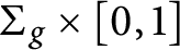
This paper concerns the chord index and its applications in virtual knot theory and twisted knot theory. Virtual knot theory, which was introduced by L. Kauffman in [29], studies the embeddings of
$S^1$
 in
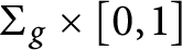
$\Sigma _g\times [0, 1]$
in
$\Sigma _g\times [0, 1]$
 up to isotopy and stabilizations. Here,
$\Sigma _g$
up to isotopy and stabilizations. Here,
$\Sigma _g$
 denotes a closed orientable surface with genus g. When
$g=0$
denotes a closed orientable surface with genus g. When
$g=0$
 , virtual knot theory reduces to the classical knot theory. It was first observed by Kauffman [Reference Kauffman30] that each real crossing point of a virtual knot can be assigned with a parity, and a kind of self-linking number, the odd writhe, was proved to be a virtual knot invariant. Later this idea was extended by Mantutov [Reference Manturov35]. The notion of chord index was independently introduced in [Reference Cheng and Gao8, Reference Dye12, Reference Im, Kim and Lee20, Reference Kauffman31, Reference Satoh and Taniguchi42], which assigns an integer to each real crossing point such that the parity of it exactly equals the parity that introduced by Kauffman.
The chord index has several applications in virtual knot theory. For example, one can construct finite type invariants of virtual knots by using chord index. A well-known result in finite type invariant theory is that, for classical knots, there exists no finite type invariant of degree one. However, for virtual knots, this is not the case. In [Reference Sawollek44], Sawollek used a degree one finite type invariant to distinguish between a virtual knot and its inverse. Later in [Reference Henrich18], Henrich defined three degree one finite type invariants for virtual knots, and the strongest one is a “universal” degree one finite type invariant for virtual knots (do not confuse this “universal” invariant with the Kontsevich integral [Reference Kontsevich33], we refer the reader to [Reference Henrich18] for the precise definition of this “universal” finite type invariant). Recently, the three loop isotopy invariant was introduced by M. Chrisman and H. Dye in [Reference Chrisman and Dye10], which turns out to be a finite type invariant of degree two.
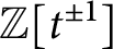
Besides the finite type invariant, one can also use the chord index to enhance some known knot invariant, for example the Jones polynomial. By ignoring all virtual crossing points, the classical Jones polynomial can be naturally defined for virtual knots with the help of Kauffman bracket. We remark that for a classical knot K, the Jones polynomial
$V_K(t)$
 takes value in
$\mathbb {Z}[t^{\pm 1}]$
takes value in
$\mathbb {Z}[t^{\pm 1}]$
 . However, for a virtual knot K, the Jones polynomial of K takes value in
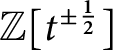
$\mathbb {Z}[t^{\pm \frac {1}{2}}]$
. However, for a virtual knot K, the Jones polynomial of K takes value in
$\mathbb {Z}[t^{\pm \frac {1}{2}}]$
 . Therefore, if
$V_K(t)$
. Therefore, if
$V_K(t)$
 contains nonzero coefficient for some term
$t^{\frac {n}{2}}$
contains nonzero coefficient for some term
$t^{\frac {n}{2}}$
 (n is odd), then we conclude that K is not classical. On the other hand, when K is a proper alternating virtual knot diagram, N. Kamada proved that the span of
$V_K(t)=c(K)-g(K)$
(n is odd), then we conclude that K is not classical. On the other hand, when K is a proper alternating virtual knot diagram, N. Kamada proved that the span of
$V_K(t)=c(K)-g(K)$
 [Reference Kamada25], here
$c(K)$
[Reference Kamada25], here
$c(K)$
 and
$g(K)$
and
$g(K)$
 denote the crossing number and supporting genus of K respectively. Later in [Reference Manturov35] the classical Jones polynomial was generalized by Manturov to the parity skein relation polynomial invariant. Similar idea was used to define the parity arrow polynomial and its categorification [Reference Kaestner and Kauffman22]. Based on the chord index, in 2017 Im and Kim considered the Jones polynomial of the n-covering of a virtual knot, which was named as the n-th polynomial in [Reference Im and Kim19]. Roughly speaking, this polynomial is defined by applying Kauffman bracket skein resolutions on crossing points of which the indices are equal to
$kn$
denote the crossing number and supporting genus of K respectively. Later in [Reference Manturov35] the classical Jones polynomial was generalized by Manturov to the parity skein relation polynomial invariant. Similar idea was used to define the parity arrow polynomial and its categorification [Reference Kaestner and Kauffman22]. Based on the chord index, in 2017 Im and Kim considered the Jones polynomial of the n-covering of a virtual knot, which was named as the n-th polynomial in [Reference Im and Kim19]. Roughly speaking, this polynomial is defined by applying Kauffman bracket skein resolutions on crossing points of which the indices are equal to
$kn$
 for some integer k. We remark that the idea of n-covering was first proposed by Turaev [Reference Turaev46]. Recently, a characterization of the n-covering of virtual knots was given by T. Nakamura, Y. Nakanishi, and S. Satoh [Reference Nakamura, Nakanishi and Satoh39].
The main aim of this paper is to provide some new applications of the chord index in virtual knot theory and its extension, the twisted knot theory. More precisely, we introduce the notion of indexed quandle. Roughly speaking, an indexed quandle is a set with a sequence of binary operations (indexed by
$\mathbb {Z}$
 ) that satisfies certain axioms. When all operations coincide the indexed quandle reduces to the classical quandle structure, which was first introduced in [Reference Joyce21, Reference Matveev36]. Therefore, the indexed quandle can be thought of as an extension of the classical quandle. For each virtual knot
$K,$
) that satisfies certain axioms. When all operations coincide the indexed quandle reduces to the classical quandle structure, which was first introduced in [Reference Joyce21, Reference Matveev36]. Therefore, the indexed quandle can be thought of as an extension of the classical quandle. For each virtual knot
$K,$
 we define its indexed knot quandle, denoted by
$I(K)$
we define its indexed knot quandle, denoted by
$I(K)$
 . This invariant is equivalent to the fundamental quandle of K when K is a classical knot. But for virtual knots, we give some examples to show that it contains much more information than the fundamental quandle. In particular, with a given finite indexed quandle
$Q,$
. This invariant is equivalent to the fundamental quandle of K when K is a classical knot. But for virtual knots, we give some examples to show that it contains much more information than the fundamental quandle. In particular, with a given finite indexed quandle
$Q,$
 one can define the coloring invariant
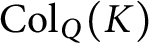
$\text {Col}_Q(K)$
one can define the coloring invariant
$\text {Col}_Q(K)$
 by counting the homomorphisms from
$I(K)$
by counting the homomorphisms from
$I(K)$
 to Q. As an analogue of the quandle cocycle invariants [Reference Carter, Jelsovsky, Kamada, Langford and Saito4], we define the indexed quandle cocycle invariants. Some examples are given to reveal that this cocycle invariant is more powerful than the coloring invariant.
In Section 4, the definition of the chord index is revisited. We want to understand what is a chord index essentially. For this purpose, we introduce the chord index axioms, which can be regarded as an extension of the parity axioms introduced by Manturov in [Reference Manturov35]. In particular, this definition can be used to nontrivially extend the notion of chord index from virtual knots to virtual links. As a concrete example, for each given finite biquandle, we construct an associated index, which can be regarded as a particular biquandle cocycle. A new virtual link invariant follows directly from this kind of chord index. Several examples are provided to explain how to calculate this associated virtual link invariant.
The last section is devoted to investigating the chord index and its applications in twisted knot theory.
2 Virtual Knot Theory and Chord Index
2.1 A Brief Review of Virtual Knots
Let
$\Sigma _g$
 be a closed orientable surface with genus g and let K be an embedded circle in
$\Sigma _g\times [0, 1]$
be a closed orientable surface with genus g and let K be an embedded circle in
$\Sigma _g\times [0, 1]$
 . Assume we have another embedded circle
$K'\subset \Sigma _{g'}\times [0, 1]$
. Assume we have another embedded circle
$K'\subset \Sigma _{g'}\times [0, 1]$
 , we say K and
$K'$
, we say K and
$K'$
 are stably equivalent if one can be obtained from the other by isotopy in the thickened surfaces, homeomorphisms of the surfaces, and addition or subtraction of empty handles. We define the virtual knots to be the stable equivalence classes of circles embedded in thickened surfaces. For a virtual knot K, the minimal genus of the surface
$\Sigma _g$
are stably equivalent if one can be obtained from the other by isotopy in the thickened surfaces, homeomorphisms of the surfaces, and addition or subtraction of empty handles. We define the virtual knots to be the stable equivalence classes of circles embedded in thickened surfaces. For a virtual knot K, the minimal genus of the surface
$\Sigma _g$
 is called the supporting genus of K. By using some classical technique in 3-manifold topology, Kuperberg [Reference Kuperberg34] proved that the embedding of a virtual knot in the minimal supporting genus thickened surface is unique. It follows that if two classical knots are stably equivalent as virtual knots, then they are also equivalent as classical knots. This implies the virtual knot theory is indeed an extension of the classical knot theory.
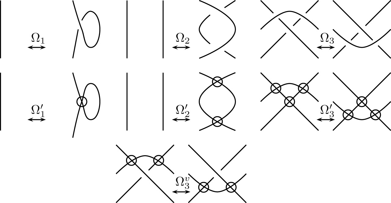
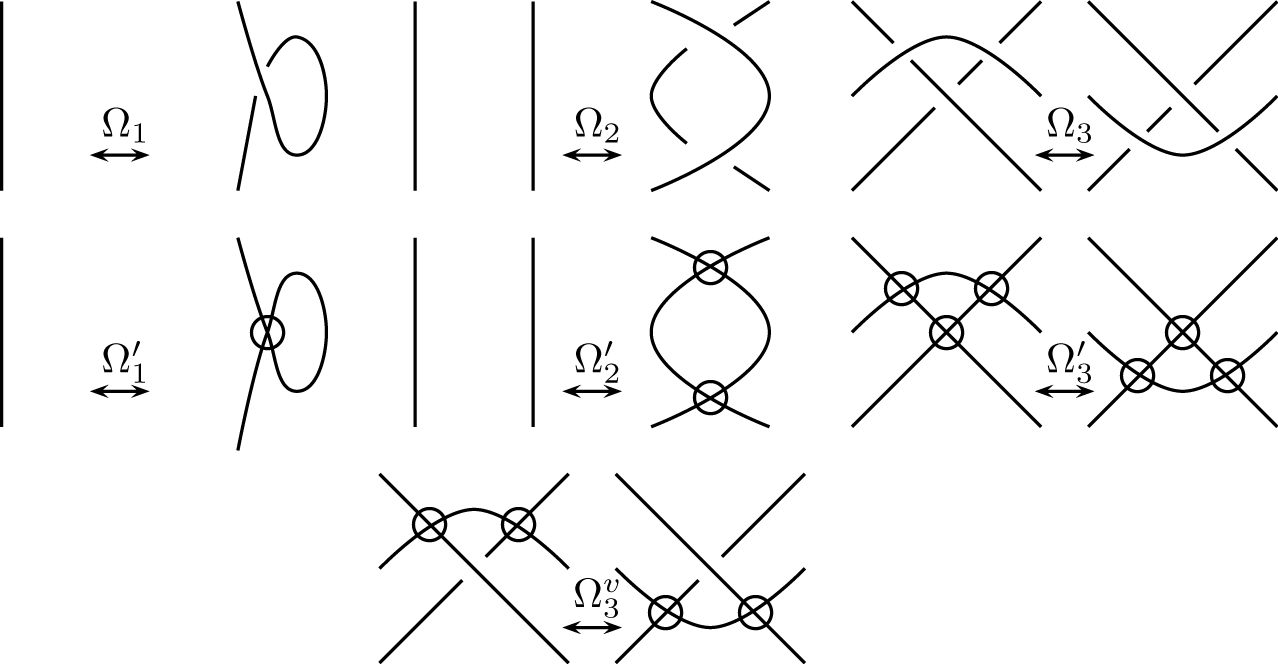
From the diagrammatic viewpoint, a virtual knot can be interpreted by virtual knot diagrams. A virtual knot diagram is an immersed circle in the plane with finitely many double points. By replacing each double point with an overcrossing, or an undercrossing, a virtual crossing (denoted by a small cricle), we obtain a virtual knot diagram. Obviously if there exists no virtual crossing the virtual knot diagram represents a classical knot. We say a pair of virtual knot diagrams are equivalent if they can be connected by a sequence of generalized Reidemeister moves, see Figure 1. Now we can define virtual knots as the equivalence classes of virtual knot diagrams up to generalized Reidemeister moves.
Generalized Reidemeister moves.
The two definitions above are closely related. Assume we have an embedded circle in a thickened surface; now consider a projection of the circle to the plane in general position. If the preimage of a double point is an overcrossing (resp.˜undercrossing) in the thickened surface, then we still use an overcrossing (resp.˜undercrossing) to denote it. If the two strands of the preimage of a double point locate in two different levels, then we use a virtual crossing to denote it. In other words, the virtual crossings can be regarded as artifacts of the projection of the surface to the plane. The readers are referred to [Reference Kauffman29] for more details. Conversely, suppose we have a virtual knot diagram K on the plane. By taking one-point compactification of the plane we obtain a virtual knot diagram on
$S^2$
 . For each virtual crossing, we add a 2-handle locally to eliminate the crossing. Finally, we obtain an embedded circle in
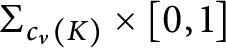
$\Sigma _{c_v(K)}\times [0, 1]$
. For each virtual crossing, we add a 2-handle locally to eliminate the crossing. Finally, we obtain an embedded circle in
$\Sigma _{c_v(K)}\times [0, 1]$
 , where
$c_v(K)$
, where
$c_v(K)$
 denotes the number of virtual crossings in K. The following theorem shows that the two definitions above are equivalent.
Theorem 2.1 [Reference Carter, Kamada and Saito5, Reference Kauffman29]
Two virtual knot diagrams are equivalent if and only if their corresponding surface embeddings are stably equivalent.
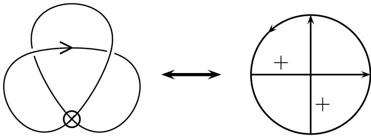
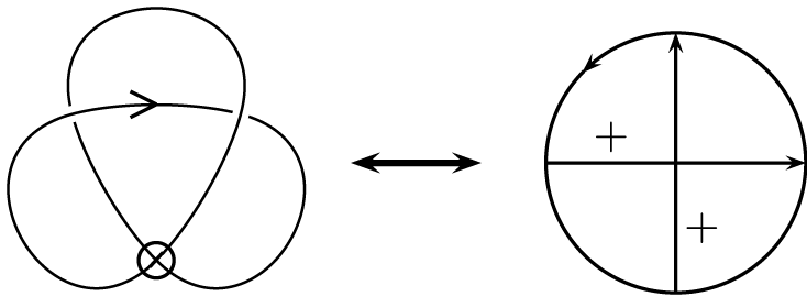
Another way to understand virtual knots is to regard them as Gauss diagrams. Let K be a virtual knot diagram that can be seen as an immersed circle in the plane. Consider the preimage of this immersed circle with an anticlockwise orientation. For each real crossing point, we draw a chord directed from the preimage of the overcrossing to the preimage of the undercrossing. Finally, we assign a sign to each chord according to the sign of the corresponding crossing point. We call this chord diagram the Gauss diagram of K and use
$G(K)$
 to denote it; see Figure 2 for a simple example. We note that all virtual crossing points are ignored on the Gauss diagram.
Virtual trefoil knot and its Gauss diagram.
Theorem 2.2 [Reference Goussarov, Polyak and Viro17]
A Gauss diagram uniquely defines a virtual knot diagram up to
$\Omega _1', \Omega _2', \Omega _3',$
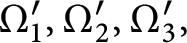 and
$\Omega _3^v$
and
$\Omega _3^v$
 .
.
Although there may exist infinitely many different virtual knot diagrams that correspond to the same Gauss diagram, we have the following correspondence between them.
Many virtual knot invariants have been discovered since the introduction of virtual knot theory. Several classical knot invariants can be directly extended to the virtual world. For example, the knot group, the knot quandle and the Jones polynomial can be similarly defined for virtual knots [Reference Kauffman29]. Some generalizations of the Alexander polynomial for virtual knots can be found in [Reference Sawollek43, Reference Silver and Williams45], and some generalizations of the Jones polynomial can be found in [Reference Dye and Kauffman13, Reference Miyazawa37, Reference Miyazawa38]. Readers should refer to [Reference Fenn, llyutko, Kauffman and Manturov14] for some recent progress and open problems in virtual knot theory.
2.2 Chord Index
Let K be a virtual knot diagram and let
$G(K)$
 be the corresponding Gauss diagram. According to the one to one correspondence between the real crossing points in K and chords in
$G(K)$
be the corresponding Gauss diagram. According to the one to one correspondence between the real crossing points in K and chords in
$G(K)$
 , we will use the same symbol to denote a real crossing in K and its corresponding chord in
$G(K)$
, we will use the same symbol to denote a real crossing in K and its corresponding chord in
$G(K)$
 . Choose a chord c in
$G(K)$
. Choose a chord c in
$G(K)$
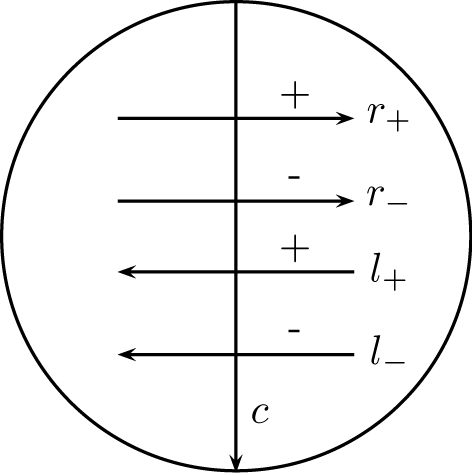
 ; we associate four integers to c as follows:
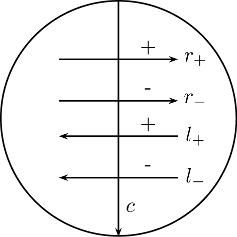
-
(a) $r_+(c)=$
 the number of positive chords crossing c from left to right;
 -
(b) $r_-(c)=$
the number of negative chords crossing c from left to right; -
(c) $l_+(c)=$
the number of positive chords crossing c from right to left; -
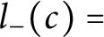
(d) $l_-(c)=$
the number of negative chords crossing c from right to left.
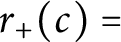
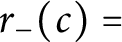
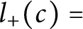
See Figure 3. Now we define the index of c as

The definition of the chord index.
Now we follow [Reference Folwaczny and Kauffman16] to give another definition of the chord index from the viewpoint of knot diagrams. Before proceeding to give the definition, we need to take a quick review of the linking number in virtual knot theory. Let
$L=K_1\cup K_2$
 be a 2-component virtual link diagram. We use Over
$(C)$
be a 2-component virtual link diagram. We use Over
$(C)$
 (resp. Under
$(C)$
(resp. Under
$(C)$
 ) to denote the set of crossings between
$K_1$
) to denote the set of crossings between
$K_1$
 and
$K_2$
and
$K_2$
 that we encounter as overcrossings (resp. undercrossings) when we travel along
$K_1$
that we encounter as overcrossings (resp. undercrossings) when we travel along
$K_1$
 . Now we define the over linking number
$lk_O(L)=\sum _{c\in \text {Over}(C)}w(c)$
. Now we define the over linking number
$lk_O(L)=\sum _{c\in \text {Over}(C)}w(c)$
 and the under linking number
$lk_U(L)=\sum _{c\in \text {Under}(C)}w(c)$
and the under linking number
$lk_U(L)=\sum _{c\in \text {Under}(C)}w(c)$
 , where
$w(c)$
, where
$w(c)$
 is the writhe of c. Note that if L is classical, we always have
$lk_O(L)=lk_U(L)$
is the writhe of c. Note that if L is classical, we always have
$lk_O(L)=lk_U(L)$
 . But when L has some virtual crossings, this is not true in general.
We turn to the definition of chord index using over linking number and under linking number. Let K be a virtual knot diagram and let c be a real crossing point of it. By smoothing c along the orientation of
$K,$
 we obtain a 2-component link
$L=K_1\cup K_2$
we obtain a 2-component link
$L=K_1\cup K_2$
 , where the order of
$K_1$
, where the order of
$K_1$
 and
$K_2$
and
$K_2$
 is indicated in Figure 4. The index of the crossing point c can be defined as:

Smooth the crossing point c.

We end this section with some useful properties of the chord index. The details of the proof can be found in, for example [Reference Cheng and Gao8, Reference Folwaczny and Kauffman16, Reference Kauffman31].
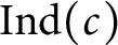
Proposition 2.3 Let K be a virtual knot diagram and c a real crossing point of it, then we have the following results:
-
(i) The two definitions of the chord index mentioned above are equivalent.
-
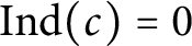
(ii) If c is isolated, i.e., no other chord has nonempty intersection with c, then $\mathrm{Ind}(c)=0$
. -
(iii) The two crossings involved in $\Omega _2$
have the same index. -
(iv) The indices of the three crossings involved in $\Omega _3$
are invariant under
$\Omega _3$
. -
(v) $\Omega _i (i=1, 2, 3)$
preserves the indices of chords that do not appear in
$\Omega _i (i=1, 2, 3)$
. -
(vi) If K contains no virtual crossings, then every crossing of K has index zero.
-
(vii) $\mathrm{Ind}(c)$
is invariant under switching some other real crossings.




2.3 Writhe Polynomial
Now we explain how to use the chord index to define a polynomial invariant of virtual knots. As before, we use K to denote a virtual knot diagram and c to denote a real crossing of K. Proposition 2.3 allows us to consider the following integers:
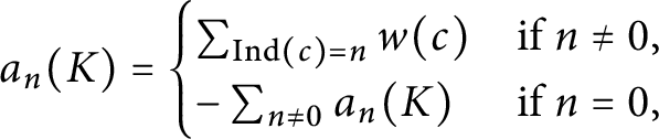
where
$w(c)$
 denotes the sign of c. We note that
$a_0$
denotes the sign of c. We note that
$a_0$
 can be also interpreted as
$\sum _{\mathrm{Ind}(c)=0}w(c)-w(K)$
can be also interpreted as
$\sum _{\mathrm{Ind}(c)=0}w(c)-w(K)$
 , here
$w(K)$
, here
$w(K)$
 denotes the writhe of K. The following theorem can be easily derived from Proposition 2.3.
Theorem 2.4 [Reference Cheng and Gao8, Reference Dye12, Reference Im, Kim and Lee20, Reference Kauffman31, Reference Satoh and Taniguchi42]
For any integer
$n\in \mathbb {Z}$
 ,
$a_n(K)$
,
$a_n(K)$
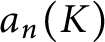 is an invariant of a virtual knot K.
For convenience, we rewrite these invariants
$\{a_n(K)\}$
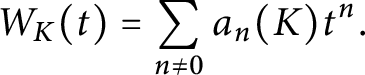
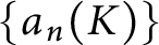 in the form of a polynomial. We define the writhe polynomial, which was introduced in [Reference Cheng and Gao8], as
Remark 2.5 The first index type invariant for virtual knots was defined by Henrich in [Reference Henrich18]. As a generalization of the odd writhe [Reference Kauffman30], the author introduced the odd writhe polynomial in [Reference Cheng6], which consists of the “odd” part of the writhe polynomial. Later, the writhe polynomial was independently introduced by several different research groups ([Reference Cheng and Gao8, Reference Dye12, Reference Im, Kim and Lee20, Reference Kauffman31, Reference Satoh and Taniguchi42]) under different names, such as affine index polynomial [Reference Kauffman31], parity writhe polynomial [Reference Im, Kim and Lee20], or n-th parity writhe [Reference Satoh and Taniguchi42]. It turns out that all of them are actually equivalent.
The writhe polynomial
$W_K(t)$
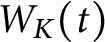 has many applications in virtual knot theory. First,
$W_K(t)=0$
has many applications in virtual knot theory. First,
$W_K(t)=0$
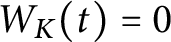 if K is classical, since all crossing points have index zero in this case. Hence, whenever
$W_K(t)\neq 0$
if K is classical, since all crossing points have index zero in this case. Hence, whenever
$W_K(t)\neq 0$
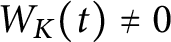 , K must be non-classical. On the other hand, the writhe polynomial is quite sensitive to some symmetries of virtual knots. For example, consider the virtual trefoil knot in Figure 2. Direct calculation shows that its writhe polynomial is
$t+t^{-1}$
, K must be non-classical. On the other hand, the writhe polynomial is quite sensitive to some symmetries of virtual knots. For example, consider the virtual trefoil knot in Figure 2. Direct calculation shows that its writhe polynomial is
$t+t^{-1}$
 ; however, the mirror image of it has writhe polynomial
$-t-t^{-1}$
; however, the mirror image of it has writhe polynomial
$-t-t^{-1}$
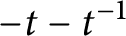 . Some examples in [Reference Cheng and Gao8] show that writhe polynomial can also be used to distinguish some virtual knots from their inverses. According to the definition of the chord index, it is evident that
$|a_n(K)| (n\neq 0)$
. Some examples in [Reference Cheng and Gao8] show that writhe polynomial can also be used to distinguish some virtual knots from their inverses. According to the definition of the chord index, it is evident that
$|a_n(K)| (n\neq 0)$
 gives a lower bound for the number of crossings with index n. However, if a crossing point has index zero, then it has no contribution to the writhe polynomial. Therefore, in general we cannot obtain any information about the number of crossing points with index zero from the writhe polynomial. For example, the index of any crossing in a classical knot diagram is zero but the writhe polynomial is also zero. One approach to overcome this problem was given recently in [Reference Cheng7]. Before ending this section, we want to remark that the writhe polynomial provides not only a lower bound for the classical crossing number, but also a lower bound for the virtual crossing number [Reference Satoh and Taniguchi42]. Recently, a necessary and sufficient condition for two virtual knots having the same writhe polynomial was given by T. Nakamura, Y. Nakanishi, and S. Satoh in [Reference Nakamura, Nakanishi and Satoh40].
3 Indexed Quandle and its Applications
3.1 A Quick Review of the Quandle Structure
To set the stage, we recall some basic notions of quandle and its generalizations.
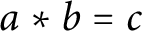
Definition 3.1 A quandle Q is a set with a binary operation
$\ast : Q\times Q\rightarrow Q$
 , which satisfies
-
(i) for all $a\in Q$
,
$a\ast a=a$
; -
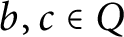
(ii) for all $b, c\in Q$
, there exists a unique
$a\in Q$
such that
$a\ast b=c$
; -
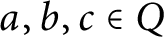
(iii) for all $a, b, c\in Q$
,
$(a\ast b)\ast c=(a\ast c)\ast (b\ast c)$
.




Here we list some examples of quandles.
-
• For any nonempty set $Q,$
one can define the trivial quandle by setting
$a\ast a=a$
for any
$a\in Q$
. -
• A conjugacy class of a group with quandle operation $a\ast b=b^{-1}ab$
is called a conjugation quandle . -
• Consider the unit sphere $S^n$
in
$\mathbb {R}^{n+1}$
, the operation
$a\ast b=2(a\cdot b)b-a$
provides a quandle structure on
$S^n$
. Here,
$\cdot $
denotes the inner product of
$\mathbb {R}^{n+1}$
.









The notion of quandle was defined by Joyce in [Reference Joyce21] (and independently by Matveev in [Reference Matveev36] with the name distributive groupoid). Given a classical knot diagram K, the knot quandle (also called fundamental quandle)
$Q(K)$
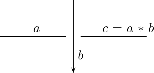
 is generated by the arcs of K and subject to the relations indicated in Figure 5. It is well known that the knot quandle distinguishes knots up to mirrors and reverses. However, similar to the knot group, in general, the knot quandle is difficult to deal with. In practise, a more easily computable invariant is the number of quandle homomorphisms from
$Q(K)$
is generated by the arcs of K and subject to the relations indicated in Figure 5. It is well known that the knot quandle distinguishes knots up to mirrors and reverses. However, similar to the knot group, in general, the knot quandle is difficult to deal with. In practise, a more easily computable invariant is the number of quandle homomorphisms from
$Q(K)$
 to a fixed finite quandle Q. We call it the coloring invariant and use
$\text {Col}_Q(K)$
to a fixed finite quandle Q. We call it the coloring invariant and use
$\text {Col}_Q(K)$
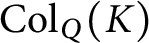 to denote it. From the viewpoint of knot diagram, a coloring assigns to each arc of the knot diagram an element of Q such that at each crossing the coloring rule indicated in Figure 5 is satisfied.
The coloring rule at each crossing.
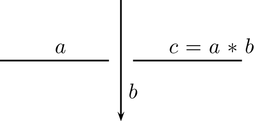
The knot quandle can be similarly defined for virtual knots. For a given virtual knot diagram, corresponding to each segment with breaks at under-crossings take a generator and corresponding to each classical crossing point take a relator as indicated in Figure 5. The reader is reminded that each segment traverses many (or maybe none) under-crossings and virtual crossings, and each virtual crossing provides no relator. However, the knot quandle is not good at distinguishing virtual knots. For example, the knot quandle of the virtual trefoil described in Figure 2 is trivial. For this reason, R. Fenn, M. Jordan-Santana and L. H. Kauffman [Reference Fenn, Jordan-Santana and Kauffman15] introduced a more general algebraic structure, say the biquandle. Note that the definition used here was suggested in [Reference Kaestner, Nelson and Selker24], which is a bit different from the original definition introduced in [Reference Fenn, Jordan-Santana and Kauffman15]. But it is easy to see that they are essentially the same.
Definition 3.2 A biquandle
$BQ$
 is a set with two binary operations
$\ast , \circ : BQ\times BQ\rightarrow BQ$
is a set with two binary operations
$\ast , \circ : BQ\times BQ\rightarrow BQ$
 such that the following axioms are satisfied:
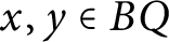
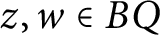
-
(i) for all $x\in BQ, x\ast x=x\circ x$
; -
(ii) for all $x, y\in BQ$
, there are unique
$z, w\in BQ$
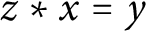
such that
$z\ast x=y$
and
$w\circ x=y$
, and the map
$S\colon (x, y)\rightarrow (y\circ x, x\ast y)$
is invertible; -
(iii) for all $x, y, z\in BQ$
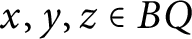
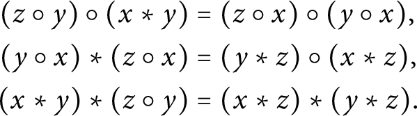
, we have $$ \begin{align*} (z\circ y)\circ(x\ast y)&=(z\circ x)\circ(y\circ x),\\ (y\circ x)\ast(z\circ x)&=(y\ast z)\circ(x\ast z),\\ (x\ast y)\ast(z\circ y)&=(x\ast z)\ast(y\ast z). \end{align*} $$



The following is a simple observation.
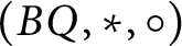
Lemma 3.3 Let
$(BQ, \ast , \circ )$
 be a biquandle and let
$x, y$
be a biquandle and let
$x, y$
 be two elements of
$BQ$
be two elements of
$BQ$
 , if
$x\ast y=y\circ x,$
, if
$x\ast y=y\circ x,$
 then
$x=y$
then
$x=y$
 .
.
Proof Taking
$z=y$
 , now the first condition in the third axiom of biquandle becomes

Since
$x\ast y=y\circ x$
 , it follows that

Recall that
$-\circ (y\circ x)$
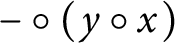 is invertible; hence, we obtain
$y\circ y=y\circ x=x\ast y$
is invertible; hence, we obtain
$y\circ y=y\circ x=x\ast y$
 . Together with the first axiom
$y\circ y=y\ast y$
. Together with the first axiom
$y\circ y=y\ast y$
 , we have
$y\ast y=x\ast y$
, we have
$y\ast y=x\ast y$
 . The desired result follows directly, because
$-\ast y$
. The desired result follows directly, because
$-\ast y$
 is invertible. ▪
Later the biquandle structure was extended by Kauffman and Manturov to the virtual biquandle [Reference Kauffman and Manturov32] by adding a relation at each virtual crossing point. The readers are referred to [Reference Carter2] for more details of quandle ideas. We will come back to the biquandle structure in Section 4.
3.2 Indexed Quandle
The parity biquandle was introduced in [Reference Kaestner and Kauffman23] and studied in [Reference Kaestner, Nelson and Selker24], where the parity was used to generalize the quandle structure. What we want to do is replace the parity with chord index.
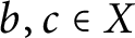
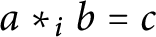
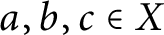
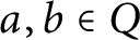
Definition 3.4 An indexed quandle is a set X with a sequence of binary operations
$\ast _i\colon X\times X\rightarrow I (i\in \mathbb {Z}),$
 which satisfy the following axioms:
-
(i) for all $a\in X, a\ast _0 a=a$
; -
(ii) for all $b, c\in X$
and
$i\in \mathbb {Z}$
, there is a unique
$a\in X$
such that
$a\ast _i b=c$
; -
(iii) for all $a, b, c\in X$
and
$i, j\in \mathbb {Z}, (a\ast _i b)\ast _j c=(a\ast _j c)\ast _i(b\ast _{j-i}c)$
.




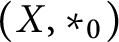
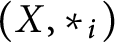
We remark that each indexed quandle
$(X, \ast _i)$
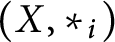 includes a quandle
$(X, \ast _0)$
includes a quandle
$(X, \ast _0)$
 . The following are some examples of the indexed quandles.
-
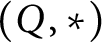
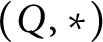
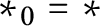
• Let $(Q, \ast )$
be a quandle; then Q can be thought of as an indexed quandle if we define
$\ast _i=\ast $
for any
$i\in \mathbb {Z}$
. -
• Let $(Q, \ast )$
be a quandle; another way to regard Q as an indexed quandle is introducing
$\ast _0=\ast $
and
$a\ast _{i} b=a (i\neq 0)$
for any
$a, b\in Q$
. -
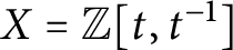
• Let $X=\mathbb {Z}[t, t^{-1}]$
be the Laurent polynomial ring. One defines
$a\ast _i b=ta+(1-t)b+i$
for any
$a, b\in \mathbb {Z}[t, t^{-1}]$
. Then
$(X, \ast _i)$
is an indexed quandle. -
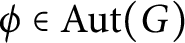
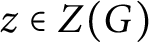
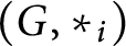
• Let G be a group. One defines $a\ast _i b=\phi (ab^{-1})bz^i$
for any
$\phi \in \text {Aut}(G)$
and
$z\in Z(G)$
(the center of G). Then
$(G, \ast _i)$
is an indexed quandle.






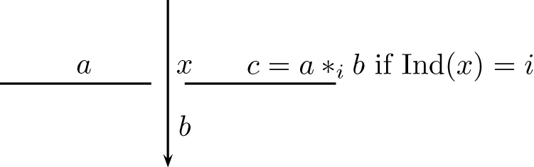
For a given virtual knot diagram K, we define the indexed knot quandle
$I(K)$
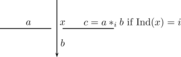
 to be the indexed quandle generated by the arcs of K, and each real crossing point gives a relation that depends on the index; see Figure 6.
The indexed coloring rule at each crossing.
Notice that when K is a classical knot diagram, the indexed knot quandle
$I(K)$
 reduces to the classical knot quandle
$Q(K)$
reduces to the classical knot quandle
$Q(K)$
 .
.
Theorem 3.5 The indexed knot quandle
$I(K)$
 is a virtual knot invariant.
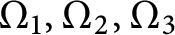
Proof It is sufficient to verify the invariance of
$I(K)$
 under
$\Omega _1, \Omega _2, \Omega _3$
under
$\Omega _1, \Omega _2, \Omega _3$
 . Since the crossing involved in
$\Omega _1$
. Since the crossing involved in
$\Omega _1$
 has index zero and the two crossing points involved in
$\Omega _2$
has index zero and the two crossing points involved in
$\Omega _2$
 have the same index, it is easy to conclude the invariance of
$I(K)$
have the same index, it is easy to conclude the invariance of
$I(K)$
 under
$\Omega _1$
under
$\Omega _1$
 and
$\Omega _2$
and
$\Omega _2$
 from the first and second axiom, respectively.
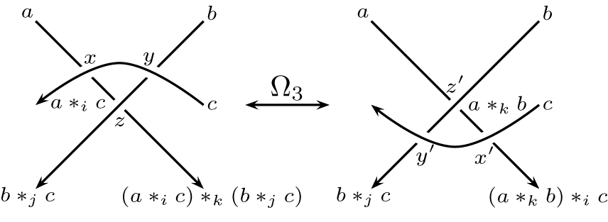
For the third Reidemeister move
$\Omega _3$
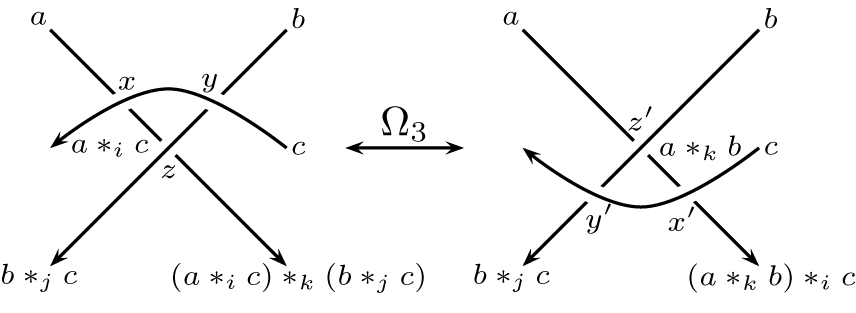
 , it is sufficient to consider the case as shown in Figure 7, where the corresponding crossing points on the two sides of
$\Omega _3$
, it is sufficient to consider the case as shown in Figure 7, where the corresponding crossing points on the two sides of
$\Omega _3$
 have the same index. We assume
$\mathrm{Ind}(x) =\mathrm{Ind}(x')=i$
have the same index. We assume
$\mathrm{Ind}(x) =\mathrm{Ind}(x')=i$
 ,
$\mathrm{Ind}(y) =\mathrm{Ind}(y')=j,$
,
$\mathrm{Ind}(y) =\mathrm{Ind}(y')=j,$
 and
$\mathrm{Ind}(z) =\mathrm{Ind}(z')=k$
and
$\mathrm{Ind}(z) =\mathrm{Ind}(z')=k$
 . Similar to the proof of Lemma 4.1 in [Reference Cheng7], it is not difficult to show that
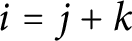
$i=j+k$
. Similar to the proof of Lemma 4.1 in [Reference Cheng7], it is not difficult to show that
$i=j+k$
 . Together with the third axiom, the invariance of
$I(K)$
. Together with the third axiom, the invariance of
$I(K)$
 can be obtained from Figure 7 directly. ▪
The invariance of
$I_K$
 under
$\Omega _3$
under
$\Omega _3$
 .
.
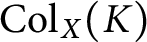
For a finite indexed quandle X, we denote by
$\text {Col}_X(K)$
 the number of homomorphisms from the indexed knot quandle
$I(K)$
the number of homomorphisms from the indexed knot quandle
$I(K)$
 to X.
to X.
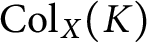
Corollary 3.6 The integer
$\text {Col}_X(K)$
 is a virtual knot invariant.
Recall that any indexed quandle
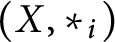
$(X, \ast _i)$
 defines the quandle
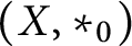
$(X, \ast _0)$
defines the quandle
$(X, \ast _0)$
 . For a classical knot K, it holds that

we have
$\text {Col}_{(X, \ast _i)}(K)=\text {Col}_{(X, \ast _0)}(K)$
 . However, this is not the case for virtual knots.
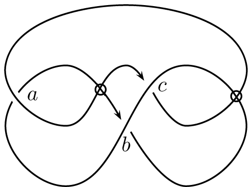
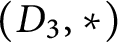
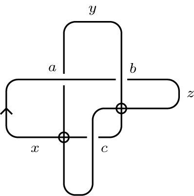
Example 3.7 Let K be a virtual knot diagram as shown in Figure 8. For the set
$D_3=\{0, 1, 2\}$
 , the operation
$i\ast j=2j-i \pmod 3 $
, the operation
$i\ast j=2j-i \pmod 3 $
 defines the quandle
$(D_3, \ast )$
defines the quandle
$(D_3, \ast )$
 , and
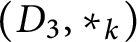
$i\ast _k j=2j-i+k\pmod { 3}$
, and
$i\ast _k j=2j-i+k\pmod { 3}$
 defines the indexed quandle
$(D_3, \ast _k)$
defines the indexed quandle
$(D_3, \ast _k)$
 . Then we have

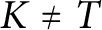
Since the trefoil knot T satisfies
$ \rm \text {Col}_{(D_3, \ast )}(T)=\text {Col}_{(D_3, \ast _k)}(T)=9$
 , we have
$K\neq T$
, we have
$K\neq T$
 .
.
The virtualization of the trefoil knot.
3.3 An Enhancement of the Coloring Invariant via Indexed Quandle 2-cocycles
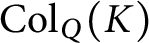
The coloring invariant
$\text {Col}_Q(K)$
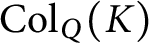
 has many applications in knot theory. For example,
$\text {Col}_Q(K)$
has many applications in knot theory. For example,
$\text {Col}_Q(K)$
 can be used to provide lower bounds for braid index, tunnel number, and unknotting number [Reference Clark, Elhamdadi, Saito and Yeatman11]. However, there also exist some disadvantages to
$\text {Col}_Q(K)$
can be used to provide lower bounds for braid index, tunnel number, and unknotting number [Reference Clark, Elhamdadi, Saito and Yeatman11]. However, there also exist some disadvantages to
$\text {Col}_Q(K)$
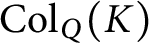 . For instance, for any finite quandle Q,
$\text {Col}_Q(K)$
. For instance, for any finite quandle Q,
$\text {Col}_Q(K)$
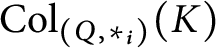
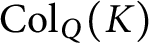 cannot distinguish the left-hand trefoil from the right-hand trefoil, since the trefoil knot is invertible. In [Reference Carter, Jelsovsky, Kamada, Langford and Saito4], J. S. Carter, D. Jelsovsky, S. Kamada, L. Langford, and M. Saito introduced the quandle (co)homology theory. In particular, with a given quandle 2(3)-cocycle, one can define an enhancement of the (shadow) coloring invariant, say the quandle cocycle invariant. There are many examples that show that these cocycle invariants are more powerful than the original coloring invariants. As an example, for some suitably chosen quandle and quandle 3-cocycle the cocycle invariant takes different values on the left-hand trefoil and the right-hand trefoil [Reference Rourke and Sanderson41]. Following the main idea of the quandle cocycle invariant we want to define the notion of indexed quandle 2-cocycle in this subsection. Analogous to the quandle 2-cocycle, each indexed quandle 2-cocycle also can be used to define a generalized invariant of
$\text {Col}_{(Q, \ast _i)}(K)$
cannot distinguish the left-hand trefoil from the right-hand trefoil, since the trefoil knot is invertible. In [Reference Carter, Jelsovsky, Kamada, Langford and Saito4], J. S. Carter, D. Jelsovsky, S. Kamada, L. Langford, and M. Saito introduced the quandle (co)homology theory. In particular, with a given quandle 2(3)-cocycle, one can define an enhancement of the (shadow) coloring invariant, say the quandle cocycle invariant. There are many examples that show that these cocycle invariants are more powerful than the original coloring invariants. As an example, for some suitably chosen quandle and quandle 3-cocycle the cocycle invariant takes different values on the left-hand trefoil and the right-hand trefoil [Reference Rourke and Sanderson41]. Following the main idea of the quandle cocycle invariant we want to define the notion of indexed quandle 2-cocycle in this subsection. Analogous to the quandle 2-cocycle, each indexed quandle 2-cocycle also can be used to define a generalized invariant of
$\text {Col}_{(Q, \ast _i)}(K)$
 .
.
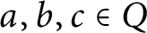
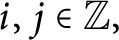
Definition 3.8 Let
$(Q, \ast _i)$
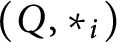 be an indexed quandle and let A be an abelian group; we call a map
$\phi : Q\times Q\rightarrow A$
be an indexed quandle and let A be an abelian group; we call a map
$\phi : Q\times Q\rightarrow A$
 an indexed quandle 2-cocycle if for any
$a, b, c\in Q$
an indexed quandle 2-cocycle if for any
$a, b, c\in Q$
 and
$i, j\in \mathbb {Z},$
and
$i, j\in \mathbb {Z},$
 it satisfies

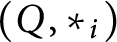
For a given virtual knot diagram K and a finite indexed quandle
$(Q, \ast _i)$
 , we choose a coloring
$f: I(K)\rightarrow (Q, \ast _i)$
, we choose a coloring
$f: I(K)\rightarrow (Q, \ast _i)$
 . For a crossing x with index i, if the three arcs around x have colors
$a, b,$
. For a crossing x with index i, if the three arcs around x have colors
$a, b,$
 and
$a\ast _i b$
and
$a\ast _i b$
 (see Figure 6), then we associate a weight
$B(x, f)=\phi (a, b)^{w(x)}$
(see Figure 6), then we associate a weight
$B(x, f)=\phi (a, b)^{w(x)}$
 with the crossing point x. As before,
$w(x)$
with the crossing point x. As before,
$w(x)$
 denotes the sign of x. Now we define the indexed quandle 2-cocycle invariant (associated with
$\phi $
denotes the sign of x. Now we define the indexed quandle 2-cocycle invariant (associated with
$\phi $
 ) to be
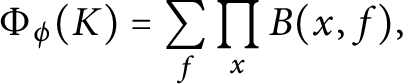
where f runs over all homomorphisms from
$I_K$
 to
$(Q, \ast _i)$
to
$(Q, \ast _i)$
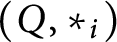 , and x runs over all real crossing points of K. Obviously, if
$\phi $
, and x runs over all real crossing points of K. Obviously, if
$\phi $
 sends each element of
$Q\times Q$
sends each element of
$Q\times Q$
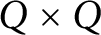 to the identity element, then
$\Phi _{\phi }(K)$
to the identity element, then
$\Phi _{\phi }(K)$
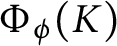 reduces to the coloring invariant
$\text {Col}_{(Q, \ast _i)}(K)$
reduces to the coloring invariant
$\text {Col}_{(Q, \ast _i)}(K)$
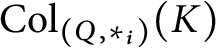 .
.
Theorem 3.9 For an indexed quandle 2-cocycle
$\phi $
 ,
$\Phi _{\phi }(K)$
,
$\Phi _{\phi }(K)$
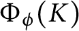 is an invariant of a virtual knot K.
Proof Since the crossing point involved in
$\Omega _1$
 has index zero, together with
$\phi (a, a)=1$
has index zero, together with
$\phi (a, a)=1$
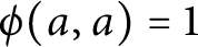 for any
$a\in Q$
for any
$a\in Q$
 , it follows that
$\Phi _{\phi }(K)$
, it follows that
$\Phi _{\phi }(K)$
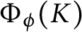 is invariant under
$\Omega _1$
is invariant under
$\Omega _1$
 . For
$\Omega _2$
. For
$\Omega _2$
 , notice that the two crossing points in
$\Omega _2$
, notice that the two crossing points in
$\Omega _2$
 have opposite signs, hence the contributions from these two crossing points cancel out. The invariance of
$\Phi _{\phi }(K)$
have opposite signs, hence the contributions from these two crossing points cancel out. The invariance of
$\Phi _{\phi }(K)$
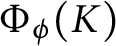 under
$\Omega _3$
under
$\Omega _3$
 can be read directly from Figure 7. ▪
Example 3.10 For the set
$\{0, 1\}$
 , the operations
$a\ast _i b=a+i$
, the operations
$a\ast _i b=a+i$
 (mod 2) define an indexed quandle
$X=(\{0, 1\}, \ast _i)$
(mod 2) define an indexed quandle
$X=(\{0, 1\}, \ast _i)$
 . Let K be the virtual knot as shown in Figure 2, and let
$K'$
. Let K be the virtual knot as shown in Figure 2, and let
$K'$
 be the virtual knot as shown in Figure 8. Then we have
$\text {Col}_X(K)=\text {Col}_X(K')=2$
be the virtual knot as shown in Figure 8. Then we have
$\text {Col}_X(K)=\text {Col}_X(K')=2$
 . On the other hand, we see that the map
$\phi : X\times X\rightarrow \mathbb {Z}_2$
. On the other hand, we see that the map
$\phi : X\times X\rightarrow \mathbb {Z}_2$
 defined by
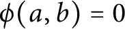
$\phi (a, b)=0$
defined by
$\phi (a, b)=0$
 for
$a=b$
for
$a=b$
 and 1 for
$a\neq b$
and 1 for
$a\neq b$
 is an indexed quandle 2-cocycle. Now we have
$\Phi _{\phi }(K)=1+1$
is an indexed quandle 2-cocycle. Now we have
$\Phi _{\phi }(K)=1+1$
 and
$\Phi _{\phi }(K')=0+0$
and
$\Phi _{\phi }(K')=0+0$
 .
.
We remark that the indexed quandle 2-cocycle invariant can be extended by replacing
$\phi $
 with a sequence of homomorphisms
$\phi _i (i\in \mathbb {Z})$
with a sequence of homomorphisms
$\phi _i (i\in \mathbb {Z})$
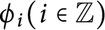 . More precisely, we use
$\psi $
. More precisely, we use
$\psi $
 to denote a sequence of
$\{\phi _i\}_{i\in \mathbb {Z}}$
to denote a sequence of
$\{\phi _i\}_{i\in \mathbb {Z}}$
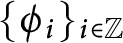 where each
$\phi _i$
where each
$\phi _i$
 represents a map from
$Q\times Q$
represents a map from
$Q\times Q$
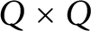 to A. We say
$\psi $
to A. We say
$\psi $
 is a generalized indexed quandle 2-cocycle if for any
$a, b, c\in Q$
is a generalized indexed quandle 2-cocycle if for any
$a, b, c\in Q$
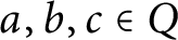 and
$i, j\in \mathbb {Z},$
and
$i, j\in \mathbb {Z},$
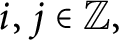 we have

With a fixed generalized indexed quandle 2-cocycle
$\psi =\{\phi _i\}_{i\in \mathbb {Z}}$
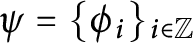 and a coloring f, we associate a weight
$\mathfrak {B}(x, f)=\phi _i(a, b)^{w(x)}$
and a coloring f, we associate a weight
$\mathfrak {B}(x, f)=\phi _i(a, b)^{w(x)}$
 with the crossing point x in Figure 6. Now we define the generalized indexed quandle 2-cocycle invariant as follows:
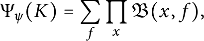
where the product takes over all crossing points and the sum takes over all colorings. In the same way, one can prove that
$\Psi _{\psi }(K)$
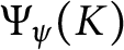 is a virtual knot invariant.
We end this section with a simple example of the generalized indexed quandle 2-cocycle invariant. Consider the indexed quandle that consists of one element a and choose the abelian group
$A=\mathbb {Z}[t, t^{-1}]$
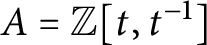 . We define a generalized indexed quandle 2-cocycle
$\psi =\{\phi _i\}$
. We define a generalized indexed quandle 2-cocycle
$\psi =\{\phi _i\}$
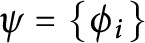 by letting
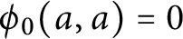
$\phi _i(a, a)=t^i (i\neq 0)$
by letting
$\phi _i(a, a)=t^i (i\neq 0)$
 and
$\phi _0(a, a)=0$
and
$\phi _0(a, a)=0$
 . Note that there exists only one coloring. Now the generalized indexed quandle 2-cocycle invariant can be read as

which is exactly the writhe polynomial we discussed in Section 2. It means that the writhe polynomial can be understood as a special case of the generalized indexed quandle cocycle invariant.
3.4 Abelian Extensions of Indexed Quandle by 2-cocycles
In group theory, it is well known that there is a one to one correspondence between the set of isomorphism classes of central extensions of G by A and the cohomology group
$H^2(G, A)$
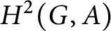 . The analogous relation between quandle extensions and quandle 2-cocycles was given by J. S. Carter et al in [Reference Carter, Elhamdadi, Nikiforou and Saito3]. In this subsection, we want to explore the relation between the extensions of indexed quandles and the generalized indexed quandle 2-cocycles.
For an indexed quandle
$(Q, \ast _i)$
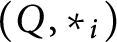 , an abelian group
$A,$
, an abelian group
$A,$
 and a sequence of maps
$\psi =\{\phi _i:Q\times Q\rightarrow A, i\in \mathbb {Z}\}$
and a sequence of maps
$\psi =\{\phi _i:Q\times Q\rightarrow A, i\in \mathbb {Z}\}$
 , we define a set
$E(Q, A, \psi )=A\times Q$
, we define a set
$E(Q, A, \psi )=A\times Q$
 equipped with a sequence of binary operations

The following proposition says
$E(Q, A, \psi )$
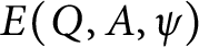 is an indexed quandle if and only if
$\psi $
is an indexed quandle if and only if
$\psi $
 is a generalized indexed quandle 2-cocycle. In this case, we say the set
$E(Q, A, \psi )$
is a generalized indexed quandle 2-cocycle. In this case, we say the set
$E(Q, A, \psi )$
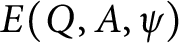 is an abelian extension of
$(Q, \ast _i)$
is an abelian extension of
$(Q, \ast _i)$
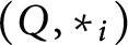 .
.
Proposition 3.11
$E(Q, A, \psi )$
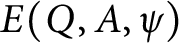 is an indexed quandle if and only if
$\psi $
is an indexed quandle if and only if
$\psi $
 is a generalized indexed quandle 2-cocycle.
Proof We assume
$\psi $
 is a generalized indexed quandle 2-cocycle. Recall that this means that for any
$x_1, x_2, x_3$
is a generalized indexed quandle 2-cocycle. Recall that this means that for any
$x_1, x_2, x_3$
 of
$Q,$
of
$Q,$
 we have

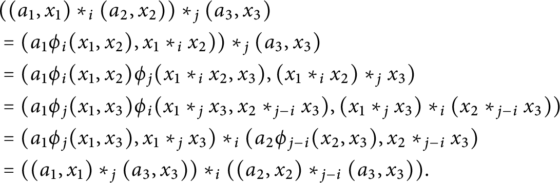
First, note that

Next, it suffices to prove

One computes
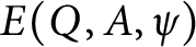
Conversely, if
$E(Q, A, \psi )$
 is an indexed quandle, one can similarly prove that
$\psi $
is an indexed quandle, one can similarly prove that
$\psi $
 satisfies the 2-cocycle conditions. ▪
4 What is a Chord Index?
In previous sections, we listed several applications of the chord index in virtual knot theory. A natural question is, is it possible to define the chord index in a more general manner? Or more generally, what is a chord index indeed? Motivated by the parity axioms proposed by Manturov in [Reference Manturov35], here we introduce the chord index axioms in virtual knot theory.
Definition 4.1 Assume we have a rule that assigns an index (e.g., an integer, a polynomial, a group, etc.) to each real crossing point in a virtual link diagram. We say this rule satisfies the chord index axioms if it satisfies the following conditions:
-
(i) The real crossing point involved in $\Omega _1$
has a fixed index. -
(ii) The two real crossing points involved in $\Omega _2$
have the same index. -
(iii) There is a natural 1-1 correspondence between the real crossing points involved in $\Omega _3$
. The corresponding real crossing points have the same index. -
(iv) The index of the real crossing point involved in $\Omega _3^v$
is preserved under
$\Omega _3^v$
. -
(v) The indices of all real crossing points that are not involved in a generalized Reidemeister move are preserved under this generalized Reidemeister move.


It is easy to observe that our chord index defined in Section 2 satisfies all chord index axioms for virtual knot diagrams. As a generalization of the chord index, in [Reference Cheng7] we introduced the index function, which also satisfies all chord index axioms above. In this section we would like to provide a general construction of chord index that satisfies all chord index axioms above. Note that the chord index and the index function only can be defined for the real crossing points in a virtual knot diagram. However, the following manner also can be used to define the chord index for real crossing points in a virtual link diagram.
In our original idea of the chord index [Reference Cheng6], the chord index is deduced from a
$\mathbb {Z}$
 -coloring on the semiarcs of a knot diagram. Later in [Reference Kauffman31], Kauffman introduced the notion of flat biquandle, which provides a more general algorithm for the colorings. In particular, Kauffman proved that essentially the coloring used in [Reference Cheng6] is the unique affine linear flat biquandle. The main result of this section is to define a general chord index via biquandles.
Recall that a biquandle is a set equipped with two binary operations
$\ast $
 and
$\circ $
and
$\circ $
 (see Definition 3.2). Similar to the knot quandle, one can define the knot biquandle
$BQ_K$
(see Definition 3.2). Similar to the knot quandle, one can define the knot biquandle
$BQ_K$
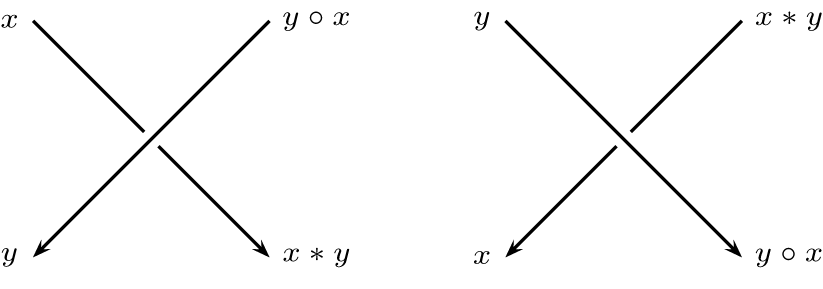
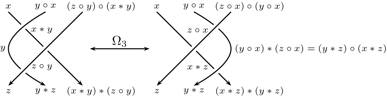
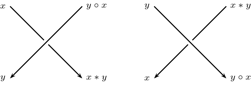
 , which is generated by all the semiarcs (a segment of the diagram from a real crossing to the next real crossing) of a virtual knot diagram but now each real crossing point offers two relations, see Figure 9. The axioms of the biquandle guarantees the invariance of
$BQ_K$
, which is generated by all the semiarcs (a segment of the diagram from a real crossing to the next real crossing) of a virtual knot diagram but now each real crossing point offers two relations, see Figure 9. The axioms of the biquandle guarantees the invariance of
$BQ_K$
 under the generalized Reidemeister moves. More precisely, the first axiom and Lemma 3.3 can be used to prove the invariance under
$\Omega _1$
under the generalized Reidemeister moves. More precisely, the first axiom and Lemma 3.3 can be used to prove the invariance under
$\Omega _1$
 . The second Reidemeister move
$\Omega _2$
. The second Reidemeister move
$\Omega _2$
 follows from the second axiom. See Figure 10 for the invariance of
$BQ_K$
follows from the second axiom. See Figure 10 for the invariance of
$BQ_K$
 under
$\Omega _3$
under
$\Omega _3$
 . Similar to the knot quandle, for any finite biquandle
$BQ$
. Similar to the knot quandle, for any finite biquandle
$BQ$
 , one can define the coloring invariant
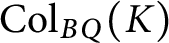
$\text {Col}_{BQ}(K)$
, one can define the coloring invariant
$\text {Col}_{BQ}(K)$
 to be
$|\text {Hom}(BQ_K, BQ)|$
to be
$|\text {Hom}(BQ_K, BQ)|$
 .
.
The coloring rule of biquandle.
Fix a finite biquandle
$BQ$
 and an abelian group A; a map
$\phi \colon BQ\times BQ\rightarrow A$
and an abelian group A; a map
$\phi \colon BQ\times BQ\rightarrow A$
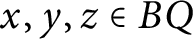
 is called a (reduced) biquandle 2-cocycle if for any
$x, y, z\in BQ$
is called a (reduced) biquandle 2-cocycle if for any
$x, y, z\in BQ$
 we have

For the sake of convenience, we introduce the universal 2-cocycle group of
$BQ$
 , which can be defined as the abelianization of

We name it in this way since each homomorphism
$\rho \colon G_{BQ}/[G_{BQ}, G_{BQ}]\rightarrow A$
 provides a biquandle 2-cocycle. More precisely, for any biquandle 2-cocycle
$\phi : BQ\times BQ\rightarrow A$
provides a biquandle 2-cocycle. More precisely, for any biquandle 2-cocycle
$\phi : BQ\times BQ\rightarrow A$
 there is a map
$\rho : G_{BQ}/[G_{BQ}, G_{BQ}]\rightarrow A$
there is a map
$\rho : G_{BQ}/[G_{BQ}, G_{BQ}]\rightarrow A$
 such that the following diagram commutes
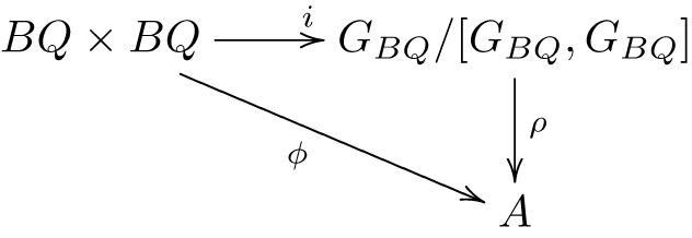
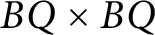
Here, i denotes the quotient map from
$BQ\times BQ$
 to
$G_{BQ}/[G_{BQ}, G_{BQ}]$
to
$G_{BQ}/[G_{BQ}, G_{BQ}]$
 .
.
Let us consider another group

Note that in
$\mathfrak {G}_{BQ}$
 we have
$(x\circ y, z\ast y)=((x\circ y)\ast ^{-1}y, z)=((x\circ y)\ast ^{-1}y, (z\circ y)\circ ^{-1}y)=(x\circ y, z\circ y)=(x, z)$
we have
$(x\circ y, z\ast y)=((x\circ y)\ast ^{-1}y, z)=((x\circ y)\ast ^{-1}y, (z\circ y)\circ ^{-1}y)=(x\circ y, z\circ y)=(x, z)$
 .
.
In general,
$\mathfrak {G}_{BQ}$
 is not an abelian group. Let K be a virtual knot diagram and let f be a coloring, we associate a weight
$\mathfrak {W}_f=(x, y)\in \mathfrak {G}_{BQ}$
is not an abelian group. Let K be a virtual knot diagram and let f be a coloring, we associate a weight
$\mathfrak {W}_f=(x, y)\in \mathfrak {G}_{BQ}$
 with the two crossing points in Figure 9. The main difference between
$G_{BQ}$
with the two crossing points in Figure 9. The main difference between
$G_{BQ}$
 and
$\mathfrak {G}_{BQ}$
and
$\mathfrak {G}_{BQ}$
 is,
$G_{BQ}$
is,
$G_{BQ}$
 requires that the sum of the contributions coming from the three crossing points on the left side of
$\Omega _3$
requires that the sum of the contributions coming from the three crossing points on the left side of
$\Omega _3$
 equals the sum of the contributions provided by the three crossing points on the right side. However, for
$\mathfrak {G}_{BQ}$
equals the sum of the contributions provided by the three crossing points on the right side. However, for
$\mathfrak {G}_{BQ}$
 , we require the contribution from each crossing point involved in
$\Omega _3$
, we require the contribution from each crossing point involved in
$\Omega _3$
 is preserved under
$\Omega _3$
is preserved under
$\Omega _3$
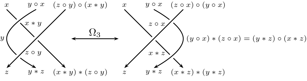
 , see Figure 10. Now we define the index (associated with
$BQ$
, see Figure 10. Now we define the index (associated with
$BQ$
 ) of a crossing point to be
$\sum _f\mathfrak {W}_f\in \mathbb {Z}\mathfrak {G}_{BQ}$
) of a crossing point to be
$\sum _f\mathfrak {W}_f\in \mathbb {Z}\mathfrak {G}_{BQ}$
 . Notice that the index does not depend on the choice of f. If there exists a homomorphism
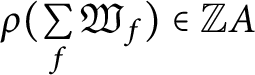
$\rho $
. Notice that the index does not depend on the choice of f. If there exists a homomorphism
$\rho $
 from
$\mathfrak {G}_{BQ}$
from
$\mathfrak {G}_{BQ}$
 to some other group A, then we obtain an induced chord index
$\rho (\sum \limits _f\mathfrak {W}_f)\in \mathbb {Z}A$
to some other group A, then we obtain an induced chord index
$\rho (\sum \limits _f\mathfrak {W}_f)\in \mathbb {Z}A$
 .
.
Biquandle coloring under
$\Omega _3$
 .
.
Example 4.2 [Reference Kauffman31]
Let
$X=(\mathbb {Z}, \ast , \circ )$
 be a biquandle, where
$x\ast y=x\circ y=x+1$
be a biquandle, where
$x\ast y=x\circ y=x+1$
 . For each virtual knot diagram there exist infinitely many colorings. In particular, if one chooses a coloring f, then any other coloring can be obtained from f by adding an integer to the assigned number on each semiarc of K. Consider a map
$\rho : \mathbb {Z}\times \mathbb {Z}\rightarrow \mathbb {Z}$
. For each virtual knot diagram there exist infinitely many colorings. In particular, if one chooses a coloring f, then any other coloring can be obtained from f by adding an integer to the assigned number on each semiarc of K. Consider a map
$\rho : \mathbb {Z}\times \mathbb {Z}\rightarrow \mathbb {Z}$
 defined by
$\rho (x, y)=y-x$
defined by
$\rho (x, y)=y-x$
 . One can naturally extend this map to a homomorphism from
$\mathfrak {G}_X$
. One can naturally extend this map to a homomorphism from
$\mathfrak {G}_X$
 to
$\mathbb {Z}[\mathbb {Z}]$
to
$\mathbb {Z}[\mathbb {Z}]$
 . We still use
$\rho $
. We still use
$\rho $
 to denote it. Now the induced chord indices of the two crossing points depicted in Figure 9 are both equal to
$\sum _{\mathbb {Z}}\rho (x, y)=\sum _{\mathbb {Z}}(y-x)$
to denote it. Now the induced chord indices of the two crossing points depicted in Figure 9 are both equal to
$\sum _{\mathbb {Z}}\rho (x, y)=\sum _{\mathbb {Z}}(y-x)$
 . It is easy to observe that essentially this is nothing but the index we defined in Section 2.
Analogous to the definition of the writhe polynomial, for a given virtual link diagram L and a fixed finite biquandle
$BQ$
 we define

Here,
$\mathfrak {g}$
 is an element of
$\mathbb {Z}\mathfrak {G}_{BQ}$
is an element of
$\mathbb {Z}\mathfrak {G}_{BQ}$
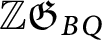 and
$w(L)$
and
$w(L)$
 denotes the writhe of L. The next theorem follows directly from our constructions above, which can be regarded as an extension of Theorem 2.4.
Theorem 4.3 Let L be a virtual link diagram; then for any finite biquandle
$BQ$
 and any
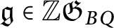
$\mathfrak {g}\in \mathbb {Z}\mathfrak {G}_{BQ}$
and any
$\mathfrak {g}\in \mathbb {Z}\mathfrak {G}_{BQ}$
 ,
$a_{\mathfrak {g}}(L)$
,
$a_{\mathfrak {g}}(L)$
 is a virtual link invariant.
The proof is left as an exercise for the reader.
Example 4.4 Consider the biquandle
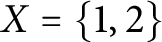
$X=\{1, 2\}$
 with operations
$1\ast i=1\circ i=1$
with operations
$1\ast i=1\circ i=1$
 and
$2\ast i=2\circ i=2 (i=1, 2)$
and
$2\ast i=2\circ i=2 (i=1, 2)$
 . In other words, X is the trivial biquandle that contains two elements. Now we have
$\mathfrak {G}_X=\mathbb {Z}\ast \mathbb {Z}$
. In other words, X is the trivial biquandle that contains two elements. Now we have
$\mathfrak {G}_X=\mathbb {Z}\ast \mathbb {Z}$
 and the generators are
$(1, 2)$
and the generators are
$(1, 2)$
 and
$(2, 1)$
and
$(2, 1)$
 . Then for any two-component virtual link
$L=K_1\cup K_2$
. Then for any two-component virtual link
$L=K_1\cup K_2$
 the link invariants defined above can be described as follows
$a_{\mathfrak {g}}(L)= \begin {cases} lk_O(L)+lk_U(L)& \text {if }\mathfrak {g}=1+1+(1, 2)+(2, 1),\\ -lk_O(L)-lk_U(L)& \text {if }\mathfrak {g}=1+1+1+1,\\ 0& \text {otherwise.} \end {cases}$

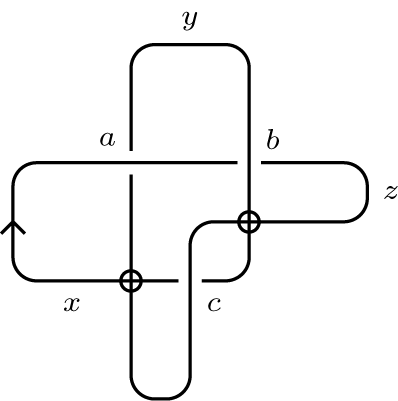
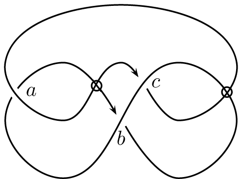
Example 4.5 As we mentioned at the beginning of this section, now we can define the chord indices for the real crossing points in a virtual link diagram. Let us consider the virtual link L in Figure 11. Choose a biquandle
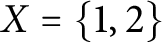
$X=\{1, 2\}$
 , and the binary operations are defined as
$1\ast i=1\circ i=2$
, and the binary operations are defined as
$1\ast i=1\circ i=2$
 and
$2\ast i=2\circ i=1 (i=1, 2)$
and
$2\ast i=2\circ i=1 (i=1, 2)$
 . It is easy to observe that in
$\mathfrak {G}_X,$
. It is easy to observe that in
$\mathfrak {G}_X,$
 we have
$1=(1, 1)=(2, 2), (1, 2)=(2, 1)$
we have
$1=(1, 1)=(2, 2), (1, 2)=(2, 1)$
 . Therefore,
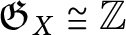
$\mathfrak {G}_X\cong \mathbb {Z}$
. Therefore,
$\mathfrak {G}_X\cong \mathbb {Z}$
 , which is generated by
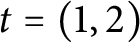
$t=(1, 2)$
, which is generated by
$t=(1, 2)$
 . Note that there exist four colorings and the indices of crossing points
$a, b, c$
. Note that there exist four colorings and the indices of crossing points
$a, b, c$
 are
$1+1+t+t, t+t+t+t, 1+1+t+t$
are
$1+1+t+t, t+t+t+t, 1+1+t+t$
 respectively. As a result we have
$a_{1+1+t+t}(L)=2$
respectively. As a result we have
$a_{1+1+t+t}(L)=2$
 and
$a_{t+t+t+t}(L)=1$
and
$a_{t+t+t+t}(L)=1$
 . As a corollary, we conclude that the real crossing number of this virtual link is 3.
Chord indices of a virtual link.
Since in general the biquandle structure is more complicated than the quandle structure, a natural thought is to replace the biquandles in our construction with quandles. Obviously, because a quandle is also a biquandle, we can still define the chord index in this case. However, the following proposition tells us it provides no new information except the coloring invariant.
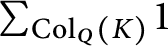
Proposition 4.6 Let Q be a finite quandle and K a virtual knot diagram; then all the crossing points of K have the same index
$\sum _{\text {Col}_Q(K)}1$
 .
.
Proof Fix a coloring f, if Q is not connected, then let us focus on the component
$Q'$
 that includes
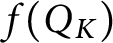
$f(Q_K)$
that includes
$f(Q_K)$
 (recall that
$Q_K$
(recall that
$Q_K$
 is connected). We claim that the group
$\mathfrak {G}_{Q'}$
is connected). We claim that the group
$\mathfrak {G}_{Q'}$
 is trivial. In fact, according to the definition of
$\mathfrak {G}_{Q'}$
is trivial. In fact, according to the definition of
$\mathfrak {G}_{Q'}$
 we have relation
$(x, z)=(x\ast y, z)$
we have relation
$(x, z)=(x\ast y, z)$
 . Since
$Q'$
. Since
$Q'$
 is connected, there exist a sequence of elements in
$Q'$
is connected, there exist a sequence of elements in
$Q'$
 , say
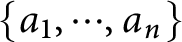
$\{a_1, \cdots , a_n\}$
, say
$\{a_1, \cdots , a_n\}$
 , such that
$(\cdots (x\ast ^{\epsilon _1} a_1)\cdots )\ast ^{\epsilon _n} a_n=z (\epsilon _i=\pm 1)$
, such that
$(\cdots (x\ast ^{\epsilon _1} a_1)\cdots )\ast ^{\epsilon _n} a_n=z (\epsilon _i=\pm 1)$
 . Now we have

which means
$\mathfrak {G}_{Q'}$
 contains only one element. The result follows. ▪
In the end of this section, we would like to remark that the chord index in Examples 4.2, 4.4, and 4.5 are all trivial for any crossing point in a classical knot diagram. It is natural to ask whether it is possible to define a nontrivial chord index for the crossing points in a classical knot diagram. On the other hand, the construction discussed in this section depends on the choice of a finite biquandle. Hence, it is not intrinsic. Recently, we provided an intrinsic construction of the chord index. The readers are referred to [Reference Cheng, Gao and Xu9] for more details.
5 Chord Index in Twisted Knot Theory
5.1 Twisted Knot Theory and Twisted Biquandle
The end of this paper is concerned with the chord index in twisted knot theory. Recall that virtual knot theory studies the embeddings of
$S^1$
 in thickened closed orientable surfaces; if we do not require that the surface must be orientable, then we encounter the twisted knot theory. Twisted knot theory was first proposed by Bourgoin [Reference Bourgoin1]. A twisted knot is a stable equivalence class of
$S^1$
in thickened closed orientable surfaces; if we do not require that the surface must be orientable, then we encounter the twisted knot theory. Twisted knot theory was first proposed by Bourgoin [Reference Bourgoin1]. A twisted knot is a stable equivalence class of
$S^1$
 in oriented 3-manifolds that are I-bundles over closed but not necessarily orientable surfaces. One main result in [Reference Bourgoin1] generalizes Kuperberg’s result [Reference Kuperberg34] from orientable surfaces to nonorientable surfaces. More precisely, Bourgoin mimicked Kuperberg’s approach to prove that the irreducible representative of a twisted knot is unique. Therefore, twisted knot theory is a proper extension of virtual knot theory.
One can also use twisted knot diagrams to illustrate twisted knots. A twisted knot diagram is a virtual knot diagram with some bars on edges. We say two twisted knot diagrams are equivalent if they are related by a sequence of generalized Reidemeister moves (see Figure 1) and twisted Reidemeister moves (see Figure 12). Similar to virtual knots, from each twisted knot diagram one can obtain an embedding of
$S^1$
 in a thickened surface, where each bar corresponds to a half-twist. It was proved in [Reference Bourgoin1] that these two definitions of twisted knots are equivalent.
Twisted Reidemeister moves.

The twisted knot group and the twisted Jones polynomial were defined in [Reference Bourgoin1]. Later N. Kamada generalized the arrow/Miyazawa polynomial to twisted knots [Reference Kamada26]. Using the similar idea of last section we want to introduce the chord index of twisted knots with a twisted biquandle. Note that the twisted quandle has been introduced by N. Kamada in [Reference Kamada26], which was motivated by the twisted group defined by Bourgoin. Here the twisted biquandle discussed below cannot be thought of as a biquandle version of the twisted quandle simply, although they reduce to biquandle and quandle respectively when the knot diagram contains no bar.
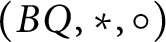
Definition 5.1 A twisted biquandle is a biquandle
$(BQ, \ast , \circ )$
 with an additional map
$f: BQ\rightarrow BQ$
with an additional map
$f: BQ\rightarrow BQ$
 that satisfies the following axioms:
-
(i) $f(y\circ x)\ast f(x\ast y)=f(y)$
, -
(ii) $f(x\ast y)\circ f(y\circ x)=f(x)$
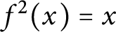
, -
(iii) $f^2(x)=x$
.


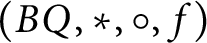
With a given finite twisted biquandle
$(BQ, \ast , \circ , f)$
 , we can define a coloring invariant
$\text {Col}_{BQ}(K)$
, we can define a coloring invariant
$\text {Col}_{BQ}(K)$
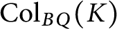 for each twisted knot K as follows. Choose a twisted knot diagram of K; for simplicity, we still use K to denote it. Assume there are
$c_r(K)$
for each twisted knot K as follows. Choose a twisted knot diagram of K; for simplicity, we still use K to denote it. Assume there are
$c_r(K)$
 real crossing points and b bars in K, now these crossings and bars split K into
$2c_r(K)+b$
real crossing points and b bars in K, now these crossings and bars split K into
$2c_r(K)+b$
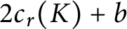 segments. For each segment, we label an element of
$BQ$
segments. For each segment, we label an element of
$BQ$
 to it such that the coloring rules described in Figure 9 are satisfied. In addition, if two segments are adjacent to the same bar, then the elements on them differ by f.
Proposition 5.2
$\text {Col}_{BQ}(K)$
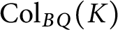 is a twisted knot invariant.
Proof The invariances of
$\text {Col}_{BQ}(K)$
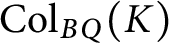 under generalized Reidemeister moves are guaranteed by the axioms of biquandle (see Definition 3.2). Hence, it is sufficient to check the twisted Reidemeister moves in Figure 12. For
$\Omega _1^t$
under generalized Reidemeister moves are guaranteed by the axioms of biquandle (see Definition 3.2). Hence, it is sufficient to check the twisted Reidemeister moves in Figure 12. For
$\Omega _1^t$
 , there is nothing need to prove. For
$\Omega _2^t$
, there is nothing need to prove. For
$\Omega _2^t$
 , the invariance of
$\text {Col}_{BQ}(K)$
, the invariance of
$\text {Col}_{BQ}(K)$
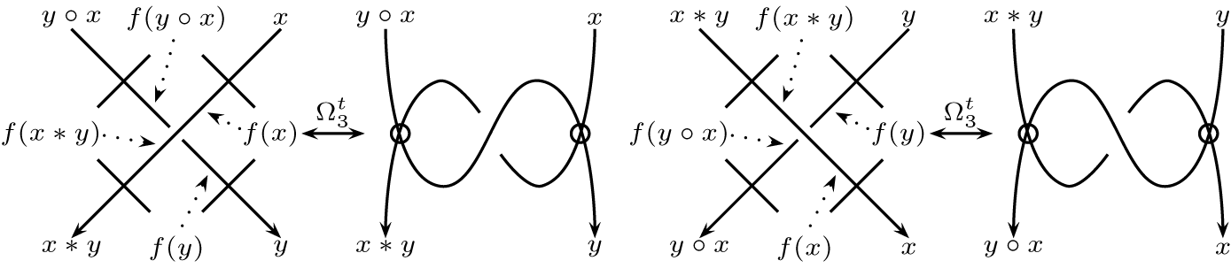
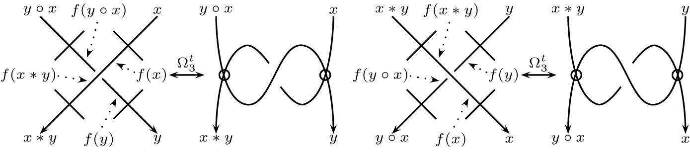
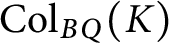 follows from the fact that f is an involution. Figure 13 explains why
$\text {Col}_{BQ}(K)$
follows from the fact that f is an involution. Figure 13 explains why
$\text {Col}_{BQ}(K)$
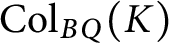 is invariant under
$\Omega _3^t$
is invariant under
$\Omega _3^t$
 . ▪
. ▪
The invariance of
$\text {Col}_{BQ}(K)$
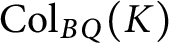 under
$\Omega _3^t$
under
$\Omega _3^t$
 .
.
In next subsection, we will focus on a special twisted biquandle
$(\mathbb {Z}, a\ast b=a\circ b=a+1, f(a)=-a)$
 . We will show how to associate an index for each real crossing point via this twisted biquandle.
5.2 A Concrete Example of Chord Index for Twisted Knots
We consider the colorings of twisted knots using twisted biquandle
$(\mathbb {Z}, a\ast b=a\circ b=a+1, f(a)=-a)$
 . A naive observation is the parity of the number of bars is preserved under twisted Reidemeister moves. For example, if a twisted knot diagram contains an odd number of bars then it can not represent a virtual knot. We continue our discussion in two cases.
First, let us consider a twisted knot K which has an odd number of bars. In this case, we have the following result.
Lemma 5.3 Let K be a twisted knot diagram; if there are an odd number of bars in K, then the coloring is unique.
Proof Assume K has
$2n-1$
 bars, denoted by
$b_1, \dots , b_{2n-1}$
bars, denoted by
$b_1, \dots , b_{2n-1}$
 . We use
$e_1, \cdots , e_{2n-1}$
. We use
$e_1, \cdots , e_{2n-1}$
 to denote the edges of
$K-\{b_1, \cdots , b_{2n-1}\}$
to denote the edges of
$K-\{b_1, \cdots , b_{2n-1}\}$
 , where the order of
$e_1, \cdots , e_{2n-1}$
, where the order of
$e_1, \cdots , e_{2n-1}$
 is consistent with the orientation of K. Consider an edge
$e_i$
is consistent with the orientation of K. Consider an edge
$e_i$
 , we use
$o_+(e_i), o_-(e_i), u_+(e_i), u_-(e_i)$
, we use
$o_+(e_i), o_-(e_i), u_+(e_i), u_-(e_i)$
 to denote the number of positive overcrossings, negative overcrossings, positive undercrossings, and negative undercrossings on
$e_i,$
to denote the number of positive overcrossings, negative overcrossings, positive undercrossings, and negative undercrossings on
$e_i,$
 respectively. Then we assign an integer
$s(e_i)=u_+(e_i)+o_-(e_i)-u_-(e_i)-o_+(e_i)$
respectively. Then we assign an integer
$s(e_i)=u_+(e_i)+o_-(e_i)-u_-(e_i)-o_+(e_i)$
 to
$e_i$
to
$e_i$
 .
.
Recall that by a coloring, we mean an assignment of integers to the segments that are obtained from K by deleting all real crossing points and bars. Along the direction of K, denote the segment adjoint to
$b_1$
 by a. Notice that according to the coloring rules, when we assign an integer k to
$a,$
by a. Notice that according to the coloring rules, when we assign an integer k to
$a,$
 the coloring of any other segment can be derived from the coloring on a. If a coloring is well defined, then the derived coloring on a must equal k. This can be described by the following equation:
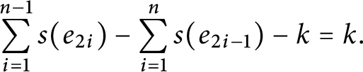
Since

It follows that
$\sum _{i=1}^{n-1}s(e_{2i})-\sum _{i=1}^{n}s(e_{2i-1})$
 is even, which means that k has a unique solution. ▪
Now we know that for any twisted knot K there is a unique coloring by using the twisted biquandle
$(\mathbb {Z}, a\ast b=a\circ b=a+1, f(a)=-a)$
 . If the colors on the four segments around a crossing c are depicted as that in Figure 9, then we define the index of c to be
$\mathrm{Ind}(c)=y-x$
. If the colors on the four segments around a crossing c are depicted as that in Figure 9, then we define the index of c to be
$\mathrm{Ind}(c)=y-x$
 . As before, we define

The following theorem is an analogue of Theorem 2.4 for twisted knots with an odd number of bars.
Theorem 5.4 Let K be a twisted knot with an odd number of bars; then each
$a_n(K)$
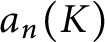 is a twisted knot invariant. Or equivalently, the polynomial
$T_o(K)=\sum _{n\in \mathbb {Z}}a_n(K)t^n$
is a twisted knot invariant. Or equivalently, the polynomial
$T_o(K)=\sum _{n\in \mathbb {Z}}a_n(K)t^n$
 is a twisted knot invariant.
Proof The invariance of
$a_n(K)$
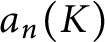 under the generalized Reidemeister moves follows directly from Proposition 2.3. For
$\Omega _1^t$
under the generalized Reidemeister moves follows directly from Proposition 2.3. For
$\Omega _1^t$
 and
$\Omega _2^t,$
and
$\Omega _2^t,$
 there is nothing need to prove. For
$\Omega _3^t$
there is nothing need to prove. For
$\Omega _3^t$
 , the proof can be read from Figure 13 by taking
$a\ast b=a\circ b=a+1$
, the proof can be read from Figure 13 by taking
$a\ast b=a\circ b=a+1$
 and
$f(a)=-a$
and
$f(a)=-a$
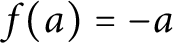 . ▪
. ▪
Now we turn to the twisted knots with an even number of bars. Note that this set contains all virtual knots, and hence all classical knots. Let K be a twisted knot with
$2n$
 bars, denoted by
$b_1, \dots , b_{2n}$
bars, denoted by
$b_1, \dots , b_{2n}$
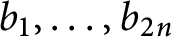 . These bars divides the knot diagram K into
$2n$
. These bars divides the knot diagram K into
$2n$
 edges, say
$e_1, \cdots , e_{2n}$
edges, say
$e_1, \cdots , e_{2n}$
 , where the order of
$e_1, \dots , e_{2n}$
, where the order of
$e_1, \dots , e_{2n}$
 agrees with the direction of K. For each edge
$e_i$
agrees with the direction of K. For each edge
$e_i$
 the assigned integer
$s(e_i)$
the assigned integer
$s(e_i)$
 can be defined as above.
Lemma 5.5
$S(K)=|\sum _{i=1}^ns(e_{2i-1})-\sum _{i=1}^ns(e_{2i})|$
 is invariant under the generalized Reidemeister moves and twisted Reidemeister moves.
Proof First, note that
$S(K)$
 does not depend on the choice of the first edge
$e_1$
does not depend on the choice of the first edge
$e_1$
 ; hence, it is welldefined. Let us consider the generalized Reidemeister moves and twisted Reidemeister moves individually.
-
• $\Omega _1$
: assume
$\Omega _1$
is taken on
$e_i$
; then
$e_i$
adds a new overcrossing and a new undercrossing which have the same writhe. Therefore,
$s(e_i)$
is preserved. -
• $\Omega _2$
: in this case, there are two edges, say
$e_i, e_j$
, where
$e_i$
adds a pair of new overcrossings with opposite signs and
$e_j$
adds a pair of new undercrossings with opposite signs. Hence both
$s(e_i)$
and
$s(e_j)$
are invariant. -
• $\Omega _3$
: it is easy to observe that for each edge involved in
$\Omega _3$
only the positions of two crossing points are switched. -
• $\Omega _1', \Omega _2', \Omega _3', \Omega _3^v, \Omega _1^t$
: nothing needs to be proved in these cases. -
• $\Omega _2^t$
: we use
$e_i^l (1\leq i\leq 2n+2)$
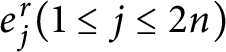
and
$e_j^r (1\leq j\leq 2n)$
to denote the edges on the left side and right side of
$\Omega _2^t,$
respectively (see Figure 12). Without loss of generality, assume the edge on the right side of
$\Omega _2^t$
is
$e_{2n}^r$
. Then the three edges on the left side of
$\Omega _2^t$
are
$e_{2n}^l, e_{2n+1}^l, e_{2n+2}^l$
. Note that
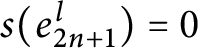
$s(e_{2n}^l)+s(e_{2n+2}^l)=s(e_{2n}^r)$
and
$s(e_{2n+1}^l)=0$
. The result follows. -
• $\Omega _3^t$
: let us consider the two local diagrams on the left side of Figure 13, say K and
$K'$
. We use
$e_i$
and
$e_i'$
to denote the edges of K and
$K'$
respectively. Let
$e_i'$
be the edge that contains the curve that begins with
$y\circ x$
and ends with y. It corresponds to three edges in K, say
$e_i, e_{i+1}, e_{i+2}$
(since S is well defined, the first edge
$e_1$
can be chosen away from the local diagram depicted in Figure 13). It is easy to observe that
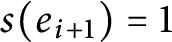
$s(e_i)+s(e_{i+2})=s(e_i')+1$
and
$s(e_{i+1})=1$
; hence, we have
$s(e_i)-s(e_{i+1})+s(e_{i+2})=s(e_i')$
. The other cases in Figure 13 can be checked in the same way.▪















According to the definition of
$S(K)$
 , it is evident that
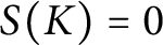
$S(K)=0$
, it is evident that
$S(K)=0$
 if K is a virtual knot. On the other hand, since
$\sum _{i=1}^ns(e_{2i-1})+\sum _{i=1}^ns(e_{2i})=0$
if K is a virtual knot. On the other hand, since
$\sum _{i=1}^ns(e_{2i-1})+\sum _{i=1}^ns(e_{2i})=0$
 , we conclude that
$S(K)$
, we conclude that
$S(K)$
 is always an even integer. The relation between the existence of colorings of K and
$S(K)$
is always an even integer. The relation between the existence of colorings of K and
$S(K)$
 is given in the following lemma.
Lemma 5.6 Consider the twisted biquandle
$(\mathbb {Z}, a\ast b=a\circ b=a+1, f(a)=-a)$
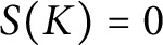
 ; there exists a coloring of K if and only if
$S(K)=0$
; there exists a coloring of K if and only if
$S(K)=0$
 .
.
Proof The proof is similar to the proof of Lemma 5.3. If a segment is assigned with an integer k, then the labels on other segments are determined according to the coloring rules. It is easy to find that there exists a coloring if and only if the equations

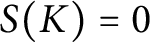
hold. Consequently, there exists a coloring of K if and only if
$S(K)=0$
 .▪
.▪
According to the proof above, we know that if
$S(K)=0,$
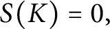 then there are infinitely many different colorings, which can be obtained by coloring a fixed segment with all integers. In order to color twisted knots with nonzero
$S(K)$
then there are infinitely many different colorings, which can be obtained by coloring a fixed segment with all integers. In order to color twisted knots with nonzero
$S(K)$
 , we replace the twisted biquandle
$(\mathbb {Z}, a\ast b=a\circ b=a+1, f(a)=-a)$
, we replace the twisted biquandle
$(\mathbb {Z}, a\ast b=a\circ b=a+1, f(a)=-a)$
 with
$(\mathbb {Z}_{S(K)}, a\ast b=a\circ b=a+1, f(a)=-a)$
with
$(\mathbb {Z}_{S(K)}, a\ast b=a\circ b=a+1, f(a)=-a)$
 . In particular, if
$S(K)=0,$
. In particular, if
$S(K)=0,$
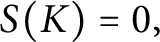 then we have
$\mathbb {Z}_{S(K)}=\mathbb {Z}$
then we have
$\mathbb {Z}_{S(K)}=\mathbb {Z}$
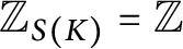 . For a twisted knot K, if we use the twisted biquandle
$(\mathbb {Z}_{S(K)}, a\ast b=a\circ b=a+1, f(a)=-a),$
. For a twisted knot K, if we use the twisted biquandle
$(\mathbb {Z}_{S(K)}, a\ast b=a\circ b=a+1, f(a)=-a),$
 then there are exactly
$S(K)$
then there are exactly
$S(K)$
 different colorings. Fix a coloring f, for the crossing point c depicted in Figure 9 we define the index of it associated with f as
$\mathrm{Ind}_f(c)=y-x \pmod {S(K)} \in \mathbb {Z}_{S(K)}$
different colorings. Fix a coloring f, for the crossing point c depicted in Figure 9 we define the index of it associated with f as
$\mathrm{Ind}_f(c)=y-x \pmod {S(K)} \in \mathbb {Z}_{S(K)}$
 . Obviously this definition depends on the choice of f, but what we need is an index that does not depend on the choice of colorings. Hence, it is necessary to study the indices of all colorings. Fortunately, there are only
$S(K)$
. Obviously this definition depends on the choice of f, but what we need is an index that does not depend on the choice of colorings. Hence, it is necessary to study the indices of all colorings. Fortunately, there are only
$S(K)$
 different colorings totally.
Let K be a twisted knot with an even number of bars, the Gauss diagram of K can be similarly defined as the virtual knots. We still use
$G(K)$
 to denote it. For any chord c in
$G(K)$
to denote it. For any chord c in
$G(K)$
 , it splits the circle into two semi-circles. Since there are totally an even number of bars in K, then either both semi-circles have an even number of bars, or both semi-circles have an odd number of bars. We use
$C_e(K)$
, it splits the circle into two semi-circles. Since there are totally an even number of bars in K, then either both semi-circles have an even number of bars, or both semi-circles have an odd number of bars. We use
$C_e(K)$
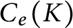 to denote all the chords of the first case and
$C_o(K)$
to denote all the chords of the first case and
$C_o(K)$
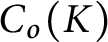 to denote all the chords of the second case.
Lemma 5.7 Choose
$c_1\in C_e(K)$
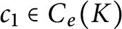 and
$c_2\in C_o(K)$
and
$c_2\in C_o(K)$
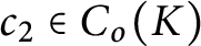 ; then
$\mathrm{Ind}_f(c_1)$
; then
$\mathrm{Ind}_f(c_1)$
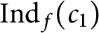 does not depend on the choice of f, and
$\mathrm{Ind}_f(c_2)$
does not depend on the choice of f, and
$\mathrm{Ind}_f(c_2)$
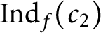 take values on all odd or all even numbers of
$\mathbb {Z}_{S(K)}$
take values on all odd or all even numbers of
$\mathbb {Z}_{S(K)}$
 .
.
Proof Recall that all colorings of K can be obtained by coloring a fixed segment a with all integers in
$\mathbb {Z}_{S(K)}$
 . Assume that when we assign
$0$
. Assume that when we assign
$0$
 to a, the index of
$c_1$
to a, the index of
$c_1$
 equals
$y_1-x_1$
equals
$y_1-x_1$
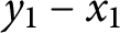 and the index of
$c_2$
and the index of
$c_2$
 equals
$y_2-x_2$
equals
$y_2-x_2$
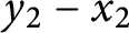 (see Figure 9). Then if a is colored by some integer k, the index of
$c_1$
(see Figure 9). Then if a is colored by some integer k, the index of
$c_1$
 turns into
$(y_1\pm k)-(x_1\pm k)=y_1-x_1$
turns into
$(y_1\pm k)-(x_1\pm k)=y_1-x_1$
 . However, the index of
$c_2$
. However, the index of
$c_2$
 becomes
$(y_2\pm k)-(x_2\mp k)=y_2-x_2\pm 2k$
becomes
$(y_2\pm k)-(x_2\mp k)=y_2-x_2\pm 2k$
 . The proof is finished. ▪
Due to the lemma above, the set
$C_o(K)$
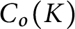 can be divided into two pieces, say
$C_o^0(K)$
can be divided into two pieces, say
$C_o^0(K)$
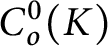 and
$C_o^1(K)$
and
$C_o^1(K)$
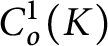 , where
$C_o^0(K)$
, where
$C_o^0(K)$
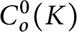 contains all the crossing points with even indices and
$C_o^1(K)$
contains all the crossing points with even indices and
$C_o^1(K)$
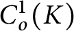 contains all the crossing points with odd indices. Since
$\mathrm{Ind}_f(c)$
contains all the crossing points with odd indices. Since
$\mathrm{Ind}_f(c)$
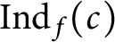 does not depend on the choice of f if
$c\in C_e(K)$
does not depend on the choice of f if
$c\in C_e(K)$
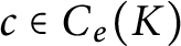 , we can simply use
$\mathrm{Ind}(c)$
, we can simply use
$\mathrm{Ind}(c)$
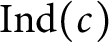 to denote it. The results of the discussion above can be summarized in the form of a polynomial:

Theorem 5.8 Let K be a twisted knot with an even number of bars; then
$T_e(K)$
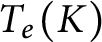 is a twisted knot invariant.
It is routine to check that

are invariant under the generalized Reidemeister moves and the twisted Reidemeister moves. Therefore we omit the proof here.
The first index type invariant of twisted knots was introduced by N. Kamada in [Reference Kamada27]. In [Reference Kamada27], N. Kamada defined two polynomials of twisted knots, denoted by
$\overline {Q}_K$
 and
$\tilde {Q}_K$
and
$\tilde {Q}_K$
 , where
$\tilde {Q}_K$
, where
$\tilde {Q}_K$
 is a refinement of
$\overline {Q}_K$
is a refinement of
$\overline {Q}_K$
 . We remark that some of our results, for instance
$\sum _{c\in C_o^0(K)}w(c)s_0$
. We remark that some of our results, for instance
$\sum _{c\in C_o^0(K)}w(c)s_0$
 and
$\sum _{c\in C_o^1(K)}w(c)s_1,$
and
$\sum _{c\in C_o^1(K)}w(c)s_1,$
 also can be found in the definition of
$\overline {Q}_K$
also can be found in the definition of
$\overline {Q}_K$
 . We end this paper with an example that explains the difference between our polynomial invariants and that introduced by N. Kamada.
A twisted knot with an odd number of bars.
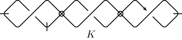
Example 5.9 Consider the twisted knot K described in Figure 14. It has three bars, hence there is a unique coloring. Direct calculation shows that
$T_o(K)=2t^2+t^{-4}-3$
 . However we remark that the chord index used in
$\overline {Q}_K$
. However we remark that the chord index used in
$\overline {Q}_K$
 and
$\tilde {Q}_K$
and
$\tilde {Q}_K$
 [Reference Kamada27] was defined in a similar manner as the linking number definition we mentioned in Section 2. For the twisted knot in Figure 14, notice that smoothing any crossing point will give us a 2-component split link. It follows that
$\overline {Q}_K$
[Reference Kamada27] was defined in a similar manner as the linking number definition we mentioned in Section 2. For the twisted knot in Figure 14, notice that smoothing any crossing point will give us a 2-component split link. It follows that
$\overline {Q}_K$
 and
$\tilde {Q}_K$
and
$\tilde {Q}_K$
 are both trivial in this example.
Acknowledgment
The author is deeply grateful to the anonymous referee for her/his careful reading of this paper and providing me numerous useful corrections and suggestions. This paper was completed during the author’s visit to the George Washington University. The author appreciates their kind hospitality during his visit.