





1. Introduction
Almost all practical combustion devices involve flames situated in flowfields with both strong turbulent and and coherent, spectrally narrowband features. For example, space–time coherent disturbances are present in flows with separating shear layers, recirculating flows and vortex breakdown in swirling flows (Lieuwen Reference Lieuwen2012). In addition, confined devices have acoustic background disturbances associated with natural acoustic modes present as well (Steinberg et al. Reference Steinberg, Boxx, Stöhr, Carter and Meier2010). Hence, turbulent flames are subject to these narrowband oscillations in addition to the broadband turbulence (Lieuwen Reference Lieuwen2012; Karmarkar et al. Reference Karmarkar, Tyagi, Hemchandra and O’Connor2021).
The ‘triple decomposition’ is a common approach for describing disturbances in these environments (Hussain & Reynolds Reference Hussain and Reynolds1970). In addition to time-mean and stochastic components, a coherent component is part of such an expansion. The existence of this coherent modulation in physical quantities suggests the importance of considering the effects of phase coherence of disturbances not only on time averages, but also on ensemble-average properties of flow/flame features. For example, the turbulent flame speed is a measure of the time-averaged burning rate, but may also exhibit well-defined, phase-averaged features.
The turbulent flame speed has been extensively discussed in the literature (Clavin Reference Clavin1985; Veynante & Vervisch Reference Veynante and Vervisch2002; Driscoll Reference Driscoll2008; Poludnenko & Oran Reference Poludnenko and Oran2011), particularly in the canonical configuration of isotropic, stationary turbulent flames. It is a definition-dependent quantity and can be defined as a consumption or displacement speed (Clavin & Joulin Reference Clavin and Joulin1983; Poinsot, Echekki & Mungal Reference Poinsot, Echekki and Mungal1992), quantifying the reactant consumption rate per unit volume or the average velocity normal to some iso-progress variable contour, respectively.
In the presence of both broadband turbulent fluctuations and coherent large-scale disturbances, the flame has two distinct sources of wrinkles and multiple length scales, as depicted in figure 1. These length scales are associated with both the size of a wrinkle as well as its ‘wavelength’.
The turbulent wrinkles can be characterised by a flame brush thickness $\lambda _{\zeta ,t}$
and the convective wavelength is
$\lambda _{\zeta ,t}$
and the convective wavelength is $\lambda _{c}=U_{0}/f_{0}$
, where
$\lambda _{c}=U_{0}/f_{0}$
, where $U_{0}$
and
$U_{0}$
and $f_{0}$
denote nominal mean axial velocity and forcing frequency, respectively. Humphrey, Emerson & Lieuwen (Reference Humphrey, Emerson and Lieuwen2018) estimated the flame brush thickness as
$f_{0}$
denote nominal mean axial velocity and forcing frequency, respectively. Humphrey, Emerson & Lieuwen (Reference Humphrey, Emerson and Lieuwen2018) estimated the flame brush thickness as $\lambda _{\zeta ,t}=u^{\prime}\tau _{int}$
, where
$\lambda _{\zeta ,t}=u^{\prime}\tau _{int}$
, where $u^{\prime}$
is the nominal root-mean-square velocity and
$u^{\prime}$
is the nominal root-mean-square velocity and $\tau _{int}$
is the integral turbulent time scale which is in turn estimated as
$\tau _{int}$
is the integral turbulent time scale which is in turn estimated as $R/U_{0}$
, where
$R/U_{0}$
, where $R$
is the radius of the reactant jet exit.
$R$
is the radius of the reactant jet exit.
In flows with narrowband disturbances, the consumption- or displacement-based turbulent flame speed exhibits clear variation in time at different points of the phase. In other words, the ensemble-averaged burning velocity is modulated about its time-average value. The first study to have analysed the ensemble-averaged dynamics of a flame subjected to both harmonic and stochastic contributions appears to be Hemchandra et al. (Reference Preetham and Lieuwen2007). Their numerical study clearly showed that stochastic velocity disturbances diminished the amplitude of harmonic flame wrinkles; i.e. the ensemble-averaged effect of the stochastic forcing did not average to zero. Shin & Lieuwen (Reference Shin and Lieuwen2013) and Humphrey et al. (Reference Humphrey, Emerson and Lieuwen2018) subsequently reported computational and experimental results, respectively, analysing turbulent flames subject to a harmonically oscillating flame holder. This configuration is a useful way to study the effect of turbulence on phase-averaged flame dynamics, as it eliminates other sources of spatial variation in coherent wrinkle magnitude (Shin & Lieuwen Reference Shin and Lieuwen2013; Karmarkar & O’Connor, Reference Karmarkar and O’Connor2023b
). These two studies established a clear negative correlation between the ensemble-averaged turbulent flame speed $(\langle S_{T}\rangle )$
and curvature of the ensemble-averaged flame
$(\langle S_{T}\rangle )$
and curvature of the ensemble-averaged flame $(\langle C\rangle )$
with the flame speed increasing in regions of negative curvature (Shin & Lieuwen Reference Shin and Lieuwen2013). An approximate fit for their results is of the form
$(\langle C\rangle )$
with the flame speed increasing in regions of negative curvature (Shin & Lieuwen Reference Shin and Lieuwen2013). An approximate fit for their results is of the form
 \begin{equation}\left\langle S_{T}\right\rangle =\left\langle S_{T}^{0}\right\rangle \left(1-\sigma _{T}\left\langle C\right\rangle \right).\end{equation}
Illustration of turbulent flame brush and convective wavelength scales where left and right images have small and large turbulent flame wrinkling components.

Here, $\langle S_{T}^{0}\rangle$
is the uncurved turbulent flame speed and
$\langle S_{T}^{0}\rangle$
is the uncurved turbulent flame speed and $\sigma _{T}$
quantifies the sensitivity of ensemble-averaged flame speed to curvature of the ensemble-averaged flame. Noting the analogy of this expression to laminar premixed flame dynamics,
$\sigma _{T}$
quantifies the sensitivity of ensemble-averaged flame speed to curvature of the ensemble-averaged flame. Noting the analogy of this expression to laminar premixed flame dynamics, $\sigma _{T}$
was denoted as ‘turbulent Markstein length’. Of course, there are fundamental differences between the turbulent Markstein length and its analogous laminar counterpart. First, the laminar Markstein length has a clear origin from rigorous asymptotics (Markstein Reference Markstein1964; Clavin & Williams Reference Clavin and Williams1982), whereas the above correlation was determined empirically. Second, they have completely different controlling physics with the concept of laminar Markstein length being applicable instantaneously, whereas the turbulent Markstein length only exists in an ensemble-averaged sense. In a different but related study, Lipatnikov & Chomiak (Reference Lipatnikov and Chomiak2004; Reference Lipatnikov and Chomiak2007) have also established a similar sensitivity of turbulent flame speed to large-scale flame curvature for statistically stationary spherical flames.
$\sigma _{T}$
was denoted as ‘turbulent Markstein length’. Of course, there are fundamental differences between the turbulent Markstein length and its analogous laminar counterpart. First, the laminar Markstein length has a clear origin from rigorous asymptotics (Markstein Reference Markstein1964; Clavin & Williams Reference Clavin and Williams1982), whereas the above correlation was determined empirically. Second, they have completely different controlling physics with the concept of laminar Markstein length being applicable instantaneously, whereas the turbulent Markstein length only exists in an ensemble-averaged sense. In a different but related study, Lipatnikov & Chomiak (Reference Lipatnikov and Chomiak2004; Reference Lipatnikov and Chomiak2007) have also established a similar sensitivity of turbulent flame speed to large-scale flame curvature for statistically stationary spherical flames.
While these studies have clearly demonstrated the phase-averaged variation of turbulent flames over a forcing period, a number of questions still remain. First, there is a large literature on the basic topology of time-averaged turbulent flame features, such as flame position or flame brush evolution (Lipatnikov & Chomiak Reference Lipatnikov and Chomiak2002; Driscoll Reference Driscoll2008; Kheirkhah & Gülder Reference Kheirkhah and Gülder2014; Fogla, Creta & Matalon Reference Fogla, Creta and Matalon2015; Trivedi et al. Reference Trivedi, Griffiths, Kolla, Chen and Cant2019; Tyagi et al. Reference Tyagi, Boxx, Peluso and O’Connor2020). There is a need for comparable understanding of the topology of ensemble-averaged flame position. Second, equation (1.1) was derived empirically and is clearly a first-order fit to a more complex reality. For example, Humphrey noted some distinction between the sensitivity of $\langle S_{T}\rangle$
and
$\langle S_{T}\rangle$
and $\langle C\rangle$
in regions of positive or negative
$\langle C\rangle$
in regions of positive or negative $\langle C\rangle$
, but did not elaborate. In addition, Kim et al. (Reference Kim, Kim, Aspden and Shin2023) have noted, through numerical computations, that a power-law approximation could fit the data better than the linear approximation for negative
$\langle C\rangle$
, but did not elaborate. In addition, Kim et al. (Reference Kim, Kim, Aspden and Shin2023) have noted, through numerical computations, that a power-law approximation could fit the data better than the linear approximation for negative $\langle C\rangle$
values. Moreover, this linear model assumes that there is no dynamical relationship between
$\langle C\rangle$
values. Moreover, this linear model assumes that there is no dynamical relationship between $\langle S_{T}\rangle$
and
$\langle S_{T}\rangle$
and $\langle C\rangle$
; it relates them algebraically at every time instant and implies that there are no unsteady effects. Although the existence of phase variation between flame speed and curvature is alluded to by Shin & Lieuwen (Reference Shin and Lieuwen2013), it has not been fully explored or quantified. Finally, while studies have clearly shown that the quantitative value of
$\langle C\rangle$
; it relates them algebraically at every time instant and implies that there are no unsteady effects. Although the existence of phase variation between flame speed and curvature is alluded to by Shin & Lieuwen (Reference Shin and Lieuwen2013), it has not been fully explored or quantified. Finally, while studies have clearly shown that the quantitative value of $\sigma _{T}$
can vary significantly across operating conditions, this underlying sensitivity of
$\sigma _{T}$
can vary significantly across operating conditions, this underlying sensitivity of $\sigma _{T}$
to other geometric, turbulence and forcing properties is not understood. To this end, Humphrey et al. (Reference Humphrey, Emerson and Lieuwen2018) suggested a correlation of
$\sigma _{T}$
to other geometric, turbulence and forcing properties is not understood. To this end, Humphrey et al. (Reference Humphrey, Emerson and Lieuwen2018) suggested a correlation of $\sigma _{T}$
to the ratio of turbulent flame brush thickness and coherent wrinkle wavelengths,
$\sigma _{T}$
to the ratio of turbulent flame brush thickness and coherent wrinkle wavelengths, $\lambda _{\zeta ,t}/\lambda _{c}$
, discussed above. While they had some success with this correlation, the results showed significant scatter with several prominent outlier points, clearly indicating that much more was at play than this single length-scale ratio.
$\lambda _{\zeta ,t}/\lambda _{c}$
, discussed above. While they had some success with this correlation, the results showed significant scatter with several prominent outlier points, clearly indicating that much more was at play than this single length-scale ratio.
The purpose of this study was to obtain experimental data to further analyse these questions and follows a major re-design of the Humphrey et al. (Reference Humphrey, Emerson and Lieuwen2018) facility to broaden the range of data, as well as fill in sparse points of that dataset. The rest of the paper is organised as follows. First, we describe the experimental facility including the diagnostics. Next, we detail the image and data processing methods used to evaluate ensemble-averaged flame position and velocity field. Lastly, we present the results related to ensemble-averaged flame speed, curvature and turbulent Markstein numbers followed by the conclusions from the present work.
2. Experimental methods
2.1. Experimental facility
Figure 2 shows a schematic of the experimental facility. The key design objective of the facility is to have a turbulent flow whose intensity can be controlled, as well as a means for introducing space–time coherent wrinkles on the premixed flame sheet.
(a) Schematic of experimental facility and (b) image of V-shaped flame and the direct-drive oscillating mechanism.

The atmospheric combustor consists of a mechanically forced, transversely oscillating flame holder anchoring a V-shaped, premixed, methane–air turbulent flame. The oscillations of the flame holder introduce coherent wrinkles on the flame, whose length scale is controlled by flow velocity and frequency, which convect downstream. Methane and air enter the base of the experimental rig through the inlet ports at an equivalence ratio of 0.7 ( $\pm$
2 %) and a nominal temperature of about 293 K (
$\pm$
2 %) and a nominal temperature of about 293 K ( $\pm$
1 %). After passing through the mixing plenum with ball bearings supported by a metal screen, it further mixes with a portion of the air seeded with titanium oxide (TiO2) particles (nominal diameter of 1 μm, Stokes number
$\pm$
1 %). After passing through the mixing plenum with ball bearings supported by a metal screen, it further mixes with a portion of the air seeded with titanium oxide (TiO2) particles (nominal diameter of 1 μm, Stokes number $\sim 10^{-3}$
(Mei Reference Mei1996)). Turbulence is introduced to the flow using a variable turbulence generator which allows for independent variation of mean flow velocity and turbulence intensity (ranging from 8 % to 35 %) and consists of two metal plates, one movable and one static, with pie-shaped slots (Marshall et al. Reference Marshall, Venkateswaran, Noble, Seitzman and Lieuwen2011). Turbulence intensity is controlled by the blockage ratio of the plates, which is done by rotating the movable plate to a given blockage ratio setting with a stepper motor through a connecting rod. The turbulent reactants pass through a contoured nozzle (jet diameter of 24.1 mm) generating a uniform top-hat velocity profile. An unseeded, velocity-matched (to the main flow) annular co-flow (outer diameter of 36.3 mm) surrounds the reactant jet.
$\sim 10^{-3}$
(Mei Reference Mei1996)). Turbulence is introduced to the flow using a variable turbulence generator which allows for independent variation of mean flow velocity and turbulence intensity (ranging from 8 % to 35 %) and consists of two metal plates, one movable and one static, with pie-shaped slots (Marshall et al. Reference Marshall, Venkateswaran, Noble, Seitzman and Lieuwen2011). Turbulence intensity is controlled by the blockage ratio of the plates, which is done by rotating the movable plate to a given blockage ratio setting with a stepper motor through a connecting rod. The turbulent reactants pass through a contoured nozzle (jet diameter of 24.1 mm) generating a uniform top-hat velocity profile. An unseeded, velocity-matched (to the main flow) annular co-flow (outer diameter of 36.3 mm) surrounds the reactant jet.
The forcing mechanism is connected to a heated, 0.81 mm diameter Nichrome wire which acts as a flame holder transversely bisecting the circular jet. The wire’s transverse position is oscillated by a brushless DC motor (no-load speed of 60 000 RPM) through a push rod and an off-centred cam disk. This mechanism provides a constant oscillation amplitude (0.3 mm for the data reported here) irrespective of the forcing frequency (motor RPM). This is an improvement to the previously reported speaker assembly mechanism with a frequency-dependent amplitude response (Humphrey et al. Reference Humphrey, Emerson and Lieuwen2018). A proportional–integral–derivative controller controls the speed of the motor and hence the frequency of oscillation of the flame holder.
Data were obtained with forcing frequencies from 200 to 800 Hz, mean reactant velocities from 3 to 8 m s−1 and turbulence intensities from 8 % to 35 %. The new experimental regime almost doubles the previous range of $u^{\prime}/S_{L}$
(ranging between 1 and 12) while also increasing the range of length-scale ratio,
$u^{\prime}/S_{L}$
(ranging between 1 and 12) while also increasing the range of length-scale ratio, $\lambda _{\zeta ,t}/\lambda _{C}$
, now spanning between 0.03 and 1.55 (Humphrey et al. Reference Humphrey, Emerson and Lieuwen2018).
$\lambda _{\zeta ,t}/\lambda _{C}$
, now spanning between 0.03 and 1.55 (Humphrey et al. Reference Humphrey, Emerson and Lieuwen2018).
2.2. Diagnostics
Time-resolved high-speed Mie scattering images were used both to track the flame edges (based on intensity difference in reactants and products) and to quantify the three-dimensional velocity field using high-speed stereo particle image velocimetry (PIV).
Figure 3 shows a schematic of the optical diagnostic set-up used. A vertical laser sheet with an approximate thickness of 0.8 mm was formed using a 527 nm dual-head, frequency-doubled Nd:YLF laser. Two Phantom v2640 cameras with Tokina f = 100 mm f/2.8 lenses were used to capture Mie scattering images of resolution 1024 × 976 pixels. Note that the unstretched flame thickness is approximately 0.7 mm (estimated from a one-dimensional premixed flame calculation). A total of 25 100 image pairs were obtained, resulting in 2510 forcing cycles with 10 image samples per forcing cycle. LaVision Davis PIV software was used to obtain all three velocity vectors components with a multi-pass, adaptive, cross-correlation algorithm. The first pass uses a 48 × 48 pixel interrogation window (with 50 % overlap) and two passes with a 16 × 16 pixel interrogation window with 50 % overlap. The processing parameters result in a vector spatial resolution of 8 pixels or ${\sim}$
0.44 mm. Finally, a universal outlier detection algorithm (in the same commercial software) was used to remove spurious vectors. The instantaneous velocity measurements are used to parameterise the value of turbulence intensity (e.g. for the x axis of figure 8), and so quoted
${\sim}$
0.44 mm. Finally, a universal outlier detection algorithm (in the same commercial software) was used to remove spurious vectors. The instantaneous velocity measurements are used to parameterise the value of turbulence intensity (e.g. for the x axis of figure 8), and so quoted $u^{\prime}$
values represent the root mean square of all three velocity components. Note that for turbulent displacement speed calculations that are the focus of this paper (2.2), it is only the ensemble-averaged velocity that is used, which is two-dimensional.
$u^{\prime}$
values represent the root mean square of all three velocity components. Note that for turbulent displacement speed calculations that are the focus of this paper (2.2), it is only the ensemble-averaged velocity that is used, which is two-dimensional.
Optical diagnostics set-up.

Illustration of image-processing steps to obtain ensemble-averaged flame edges. Image (c) overlays scalar progress variable field in greyscale, as well as progress variable fields of 0.3 (green), 0.5 (red) and 0.6 (blue).

To characterise the range of length scales, integral length scale was estimated using PIV data based on autocorrelation $\rho (\tau )$
of axial velocity measured at 1.5 mm above the flame holder location. The integral length scale,
$\rho (\tau )$
of axial velocity measured at 1.5 mm above the flame holder location. The integral length scale, $l_{0}$
, is hence calculated as
$l_{0}$
, is hence calculated as $l_{0}=u^{\prime}\int _{0}^{\infty }\rho (\tau ){\rm d}\tau$
. Integral length scale calculated this way averages about
$l_{0}=u^{\prime}\int _{0}^{\infty }\rho (\tau ){\rm d}\tau$
. Integral length scale calculated this way averages about $l_{0}/R=0.2\pm 0.025$
and varies by
$l_{0}/R=0.2\pm 0.025$
and varies by $\sim \pm 0.1$
across the velocities and turbulence intensities. The turbulent Reynolds number
$\sim \pm 0.1$
across the velocities and turbulence intensities. The turbulent Reynolds number $Re_{{l_{0}}}=u^{\prime}l_{0}/\nu$
ranges from 80 to 350 for the lowest to highest turbulence intensities.
$Re_{{l_{0}}}=u^{\prime}l_{0}/\nu$
ranges from 80 to 350 for the lowest to highest turbulence intensities.
2.3. Image and data processing
Key information to be extracted from these data were instantaneous flame position and velocity fields. To obtain flame position, the raw Mie scattering images were corrected for the distortion from the quartz window and the inclination of the camera ( ${\sim}9^{\circ}$
) using LaVision Davis PIV processing software. A sliding minimum operation removes unwanted reflections/background. Using pixels in a reference region outside the edge of the jet, variation in laser sheet intensity is corrected for by normalisation (Humphrey et al. Reference Humphrey, Emerson and Lieuwen2018). The corrected raw image is shown in figure 4(a). Gaussian blurring and edge-preserving bilateral filters were used in succession to remove high-frequency noise. Next, Otsu’s method (Otsu Reference Otsu1979) was used to binarise the images (see figure 4
b). Ensemble-averaged progress variable fields were obtained by averaging the binary images corresponding to the same phase with respect to the forcing cycle. The progress variable ranges from zero in the reactants to unity in the products and is opposite to the intensity fields obtained in figure 4(c). Since all the images of an ensemble correspond to the same phase, in this context, ensemble average is equivalent to phase average. Ensemble-averaged flame edge and all the quantities derived from it are calculated at a progress variable value of 0.5 (red line in figure 4
c). For reference, figure 4(c) also plots ensemble-averaged edges at progress variable values of 0.3 (green) and 0.6 (blue).
${\sim}9^{\circ}$
) using LaVision Davis PIV processing software. A sliding minimum operation removes unwanted reflections/background. Using pixels in a reference region outside the edge of the jet, variation in laser sheet intensity is corrected for by normalisation (Humphrey et al. Reference Humphrey, Emerson and Lieuwen2018). The corrected raw image is shown in figure 4(a). Gaussian blurring and edge-preserving bilateral filters were used in succession to remove high-frequency noise. Next, Otsu’s method (Otsu Reference Otsu1979) was used to binarise the images (see figure 4
b). Ensemble-averaged progress variable fields were obtained by averaging the binary images corresponding to the same phase with respect to the forcing cycle. The progress variable ranges from zero in the reactants to unity in the products and is opposite to the intensity fields obtained in figure 4(c). Since all the images of an ensemble correspond to the same phase, in this context, ensemble average is equivalent to phase average. Ensemble-averaged flame edge and all the quantities derived from it are calculated at a progress variable value of 0.5 (red line in figure 4
c). For reference, figure 4(c) also plots ensemble-averaged edges at progress variable values of 0.3 (green) and 0.6 (blue).
Representative instantaneous velocity field with instantaneous flame edge (black line) for $f_{0}=750$
Hz,
$f_{0}=750$
Hz, $U_{0}=4.2$
m s−1 and
$U_{0}=4.2$
m s−1 and $u^{\prime}/U_{0}=27\, \%$
.
$u^{\prime}/U_{0}=27\, \%$
.

Instantaneous velocity fields are reactant-conditioned by including the velocity vectors present only in the reactant side of the field. Reactant conditioning results in the number of ensembles between 700 and 2510 for ensemble-averaged velocity vectors. Ensemble-averaged velocity fields are obtained by averaging the instantaneous, reactant-conditioned velocity fields corresponding to the same phase. Time-averaged flame positions are used to define a coordinate system with the $s$
coordinate corresponding to the direction along the flame and
$s$
coordinate corresponding to the direction along the flame and $n$
coordinate corresponding to the direction normal to it, as shown in figure 6.
$n$
coordinate corresponding to the direction normal to it, as shown in figure 6.
Coordinate system defined based on time-averaged flame used in analysis to determine ensemble-averaged flame speed and curvature of the ensemble-averaged flame.

Ensemble-averaged flame position, $\langle \zeta (s,t)\rangle$
, is obtained by measuring the 0.5 progress variable contour along the
$\langle \zeta (s,t)\rangle$
, is obtained by measuring the 0.5 progress variable contour along the $n$
coordinate (see figure 6). Positive flame position is defined to be towards the reactants. Further, ensemble-averaged edges are fitted with cubic smoothing spline curves to calculate the first and second derivative of
$n$
coordinate (see figure 6). Positive flame position is defined to be towards the reactants. Further, ensemble-averaged edges are fitted with cubic smoothing spline curves to calculate the first and second derivative of $\langle \zeta (s,t)\rangle$
with respect to
$\langle \zeta (s,t)\rangle$
with respect to $s$
. The spline parameters were selected manually to have minimal smoothing and high R
2 values for the fits (> 0.99). The spline fits further reduce the noise amplification while calculating derivatives (Samareh Reference Samareh2001; Kungurtsev & Juniper Reference Kungurtsev and Juniper2019). Curvature of the ensemble-averaged flame was calculated from the following expression:
$s$
. The spline parameters were selected manually to have minimal smoothing and high R
2 values for the fits (> 0.99). The spline fits further reduce the noise amplification while calculating derivatives (Samareh Reference Samareh2001; Kungurtsev & Juniper Reference Kungurtsev and Juniper2019). Curvature of the ensemble-averaged flame was calculated from the following expression:
 \begin{equation} \left\langle C\right\rangle =-\frac{\frac{\partial ^{2}\left\langle \zeta \right\rangle }{\partial s^{2}}}{\left(1+\left(\frac{\partial \left\langle \zeta \right\rangle }{\partial s}\right)^{2}\right)^{\frac{3}{2}}},\end{equation}
where $\langle \zeta \rangle$
is the ensemble-averaged flame position.
$\langle \zeta \rangle$
is the ensemble-averaged flame position.
Turbulent flame speed can be defined as consumption speed, $S_{T,C}$
, or displacement speed,
$S_{T,C}$
, or displacement speed, $S_{T,D}$
. Here, we use the Shin et al. (Shin & Lieuwen Reference Shin and Lieuwen2013) definition of ensemble-averaged displacement turbulent flame speed,
$S_{T,D}$
. Here, we use the Shin et al. (Shin & Lieuwen Reference Shin and Lieuwen2013) definition of ensemble-averaged displacement turbulent flame speed, $S_{T,D}$
:
$S_{T,D}$
:
 \begin{equation} \left\langle S_{T,D}\right\rangle \equiv \frac{\frac{\partial \left\langle \zeta \right\rangle }{\partial t}+\left\langle u_{s}\right\rangle \frac{\partial \left\langle \zeta \right\rangle }{\partial s}-\left\langle u_{n}\right\rangle }{\left(1+\left(\frac{\partial \left\langle \zeta \right\rangle }{\partial s}\right)^{2}\right)^{\frac{1}{2}}}, \end{equation}
where $s$
and
$s$
and $n$
are the coordinates along and normal to the flame for a coordinate system aligned with the time-averaged flame position and
$n$
are the coordinates along and normal to the flame for a coordinate system aligned with the time-averaged flame position and $\langle u_{s}\rangle$
and
$\langle u_{s}\rangle$
and $\langle u_{n}\rangle$
are the reactant-conditioned velocity components along the
$\langle u_{n}\rangle$
are the reactant-conditioned velocity components along the $s$
and
$s$
and $n$
coordinates, respectively. The time derivative of
$n$
coordinates, respectively. The time derivative of $\langle \zeta (s,t)\rangle$
is calculated using weighted essentially non-oscillatory derivative algorithm (Jiang & Peng Reference Jiang and Peng2000), which can handle the discontinuities resulting from strong cusps. Note also that while the instantaneous velocity is three-dimensional, the ensemble-averaged velocity is two-dimensional. Figure 7 illustrates these post-processing steps used to calculate the ensemble-averaged flame speeds and curvature of ensemble-averaged flame.
$\langle \zeta (s,t)\rangle$
is calculated using weighted essentially non-oscillatory derivative algorithm (Jiang & Peng Reference Jiang and Peng2000), which can handle the discontinuities resulting from strong cusps. Note also that while the instantaneous velocity is three-dimensional, the ensemble-averaged velocity is two-dimensional. Figure 7 illustrates these post-processing steps used to calculate the ensemble-averaged flame speeds and curvature of ensemble-averaged flame.
Flowchart illustrating image and velocity processing steps used to calculate the turbulent displacement and consumption speeds.

The ensemble-averaged consumption flame speed is given by (Humphrey Reference Humphrey2017):
 \begin{equation} \left\langle S_{T,C}\right\rangle \equiv \frac{\left\langle S_{L}\left(t,s\right){\unicode[Arial]{x0394}} A\left(t,s\right)\right\rangle }{{\unicode[Arial]{x0394}} A_{0}\left(s\right)},\end{equation}
where $S_{L}(t,s)$
is the laminar flame speed,
$S_{L}(t,s)$
is the laminar flame speed, ${\unicode[Arial]{x0394}} A(t,s)$
is the area element of the instantaneous flame edge and
${\unicode[Arial]{x0394}} A(t,s)$
is the area element of the instantaneous flame edge and ${\unicode[Arial]{x0394}} A_{0}(s)$
is the area element of the time-averaged flame edge (see figure 6). We utilise a value of
${\unicode[Arial]{x0394}} A_{0}(s)$
is the area element of the time-averaged flame edge (see figure 6). We utilise a value of $S_{L}=$
19.6 cm s−1 (computed from one-dimensional freely propagating flame on Cantera) when computing the
$S_{L}=$
19.6 cm s−1 (computed from one-dimensional freely propagating flame on Cantera) when computing the $S_{T,C}$
value defined above.
$S_{T,C}$
value defined above.
The turbulent Markstein lengths, $\sigma _{T,D}$
and
$\sigma _{T,D}$
and $\sigma _{T,C}$
, then apply from utilising the relevant flame-speed definitions in (2.2) and (2.3), respectively.
$\sigma _{T,C}$
, then apply from utilising the relevant flame-speed definitions in (2.2) and (2.3), respectively.
2.4. Uncertainty analysis
Uncertainty in instantaneous velocity fields is estimated based on out-of-plane motion, calibration error due to manufacturing tolerance of the calibration plate and particle aliasing. The largest uncertainty in instantaneous velocity fields is approximately 18 %, estimated using a correlation statistics approach in the LaVision PIV processing software (Wieneke Reference Wieneke2015). Due to the nonlinear algorithms used in estimating ensemble-averaged flame speed and curvature of the ensemble-averaged flame and potentially large input uncertainties, standard linearised error propagation methods are impractical. Hence, uncertainties in ensemble-averaged quantities were obtained using a Monte Carlo approach. First, uncertainty in instantaneous flame position was obtained by visually comparing raw instantaneous images with the flame edge determined algorithmically. By increasing the thickness of the edge until it overlaps with the raw instantaneous edge, the uncertainty was calculated for a set of images as one standard deviation of the thickness values (Humphrey et al. Reference Humphrey, Emerson and Lieuwen2018). Synthetic progress variable fields were created using a known analytical function that simulates the same wrinkle magnitude, cusps and number of phase points of the ensemble-averaged flame edges (Humphrey et al. Reference Humphrey, Emerson and Lieuwen2018). Gaussian noise was added based on the estimated instantaneous uncertainty in flame position. Further, synthetic velocity fields were also created with the same mean axial velocity and flame position. Gaussian noise was added using the above-described uncertainty estimates for velocity field. Uncertainty was estimated using one standard deviation for ensemble-averaged quantities. Further, standard uncertainty propagation techniques based on (2.1)–(2.3) defining ensemble-averaged flame speed and curvature were used to estimate their corresponding uncertainties. Largest uncertainty in $u^{\prime}$
was found to be 3 %. Largest uncertainties in ensemble-averaged flame speed and curvature of the ensemble-averaged flame were found to be 8 % and 11 %, respectively.
$u^{\prime}$
was found to be 3 %. Largest uncertainties in ensemble-averaged flame speed and curvature of the ensemble-averaged flame were found to be 8 % and 11 %, respectively.
3. Results and discussion
Figure 8 plots ensemble-averaged edges (black line) corresponding to a particular phase of the forcing cycle for the turbulent, premixed V-shaped flame. Two instantaneous flame edges (red and magenta lines) are also overlaid. The conditions correspond to the flame holder oscillating at 750 Hz, a nominal mean axial velocity of ${\sim}$
4–5 m s−1 and increasing turbulence intensity from figures 8(a) to 8(d). Since the nominal mean axial velocity and frequency are the same, the convective wavelength defined as
${\sim}$
4–5 m s−1 and increasing turbulence intensity from figures 8(a) to 8(d). Since the nominal mean axial velocity and frequency are the same, the convective wavelength defined as $\lambda _{c}=U_{0}/f_{0}$
is essentially constant. However, note that turbulent flame brush thickness (see discussion below figure 1), which approximately scales as
$\lambda _{c}=U_{0}/f_{0}$
is essentially constant. However, note that turbulent flame brush thickness (see discussion below figure 1), which approximately scales as $\lambda _{\zeta ,t}=Ru^{\prime}/U_{0}$
, increases from figures 8(a) to 8(d). Several observations are evident. First, even as the instantaneous edges are more wrinkled with increasing turbulence, the ensemble-averaged edges are smoothed out at higher turbulence intensities. This is consistent with past results, and is attributed to the enhanced effect of kinematic restoration at higher turbulence intensities in smoothing out the ensemble-averaged wrinkles which are otherwise apparent at lower turbulence intensities (Hemchandra, Peters & Lieuwen Reference Hemchandra, Peters and Lieuwen2011; Shin & Lieuwen Reference Shin and Lieuwen2013). Second, the ensemble-averaged edge bends more towards the horizontal as a result of increased turbulent flame speed with increasing turbulence intensity. This illustrates the increase in turbulent displacement speed,
$\lambda _{\zeta ,t}=Ru^{\prime}/U_{0}$
, increases from figures 8(a) to 8(d). Several observations are evident. First, even as the instantaneous edges are more wrinkled with increasing turbulence, the ensemble-averaged edges are smoothed out at higher turbulence intensities. This is consistent with past results, and is attributed to the enhanced effect of kinematic restoration at higher turbulence intensities in smoothing out the ensemble-averaged wrinkles which are otherwise apparent at lower turbulence intensities (Hemchandra, Peters & Lieuwen Reference Hemchandra, Peters and Lieuwen2011; Shin & Lieuwen Reference Shin and Lieuwen2013). Second, the ensemble-averaged edge bends more towards the horizontal as a result of increased turbulent flame speed with increasing turbulence intensity. This illustrates the increase in turbulent displacement speed, $\langle S_{T,D}\rangle$
. Further, notice that in addition to smoother ensemble-averaged edges, the wrinkle amplitude decreases with increasing turbulence intensity. Finally, note that even at low turbulence intensities, there can be a transverse offset between ensemble-averaged and instantaneous flame edges due to mechanisms like random phase jitter and flame-angle modification (Shin & Lieuwen Reference Shin and Lieuwen2013).
$\langle S_{T,D}\rangle$
. Further, notice that in addition to smoother ensemble-averaged edges, the wrinkle amplitude decreases with increasing turbulence intensity. Finally, note that even at low turbulence intensities, there can be a transverse offset between ensemble-averaged and instantaneous flame edges due to mechanisms like random phase jitter and flame-angle modification (Shin & Lieuwen Reference Shin and Lieuwen2013).
Ensemble-averaged edges (black) and two instantaneous edges (red, magenta) for $f_{0}$
= 750 Hz, and
$f_{0}$
= 750 Hz, and $U_{0}=4.9,4.7,4.2,4.1$
m s−1 from (a) to (d), respectively.
$U_{0}=4.9,4.7,4.2,4.1$
m s−1 from (a) to (d), respectively.

Having considered the ensemble-averaged flame position, we next consider the variance in its position, quantified as the flame brush, $\lambda _{\zeta ,t}$
. Figure 9 plots the flame brush thickness, determined from the data as the distance between progress variable values of 0.3 and 0.6 as shown in figure 4(c). These results were extracted at streamwise locations corresponding to crests and troughs of the ensemble-averaged flame and averaged for each case. These specific locations were utilised as the normal to the ensemble-averaged flame position and time-averaged flame position aligned; at other points, the flame to the ensemble-averaged position evolves along the harmonic wrinkle (Karmarkar & O’Connor, Reference Karmarkar and O’Connor2023a). The overall flame brush thickness scales approximately linearly with
$\lambda _{\zeta ,t}$
. Figure 9 plots the flame brush thickness, determined from the data as the distance between progress variable values of 0.3 and 0.6 as shown in figure 4(c). These results were extracted at streamwise locations corresponding to crests and troughs of the ensemble-averaged flame and averaged for each case. These specific locations were utilised as the normal to the ensemble-averaged flame position and time-averaged flame position aligned; at other points, the flame to the ensemble-averaged position evolves along the harmonic wrinkle (Karmarkar & O’Connor, Reference Karmarkar and O’Connor2023a). The overall flame brush thickness scales approximately linearly with $u^{\prime}/S_{L}$
, consistent with a number of prior analyses of turbulent, premixed flames without harmonic forcing (Lipatnikov & Chomiak Reference Lipatnikov and Chomiak2002; Kheirkhah & Gülder Reference Kheirkhah and Gülder2014; Wabel et al. Reference Wabel, Skiba, Temme and Driscoll2017; Patyal & Matalon Reference Patyal and Matalon2022). Note, however, that there is some scatter in the results, especially at higher turbulence intensity values. This is a manifestation of the fact that the turbulent flame brush is a function of additional parameters, already noted in the context of unforced turbulent flames by Lipatnikov & Chomiak (Reference Lipatnikov and Chomiak2002). Moreover, these data were obtained with harmonic forcing, which introduces additional influence parameters, such as convective wavelength. Nonetheless, the figure also shows that the dominant parameter influencing the ensemble-averaged turbulent flame brush thickness is
$u^{\prime}/S_{L}$
, consistent with a number of prior analyses of turbulent, premixed flames without harmonic forcing (Lipatnikov & Chomiak Reference Lipatnikov and Chomiak2002; Kheirkhah & Gülder Reference Kheirkhah and Gülder2014; Wabel et al. Reference Wabel, Skiba, Temme and Driscoll2017; Patyal & Matalon Reference Patyal and Matalon2022). Note, however, that there is some scatter in the results, especially at higher turbulence intensity values. This is a manifestation of the fact that the turbulent flame brush is a function of additional parameters, already noted in the context of unforced turbulent flames by Lipatnikov & Chomiak (Reference Lipatnikov and Chomiak2002). Moreover, these data were obtained with harmonic forcing, which introduces additional influence parameters, such as convective wavelength. Nonetheless, the figure also shows that the dominant parameter influencing the ensemble-averaged turbulent flame brush thickness is $u^{\prime}/S_{L}$
, which is why the data are plotted in this manner. Note that the Humphrey et al. (Reference Humphrey, Emerson and Lieuwen2018) prior analysis used
$u^{\prime}/S_{L}$
, which is why the data are plotted in this manner. Note that the Humphrey et al. (Reference Humphrey, Emerson and Lieuwen2018) prior analysis used $u^{\prime}/U_{0}$
for scaling turbulent flame brush thickness. For the rest of our analysis, we define our turbulent flame brush thickness as
$u^{\prime}/U_{0}$
for scaling turbulent flame brush thickness. For the rest of our analysis, we define our turbulent flame brush thickness as $\lambda _{\zeta ,t}=Ru^{\prime}/S_{L}$
incorporating the effects of turbulent flow field and flame propagation.
$\lambda _{\zeta ,t}=Ru^{\prime}/S_{L}$
incorporating the effects of turbulent flow field and flame propagation.
Variation of flame brush thickness with $u^{\prime}/S_{L}$
for a range of streamwise positions along the flame (at the ensemble-averaged crests and troughs), turbulence generator settings, mean velocities and forcing frequencies.
$u^{\prime}/S_{L}$
for a range of streamwise positions along the flame (at the ensemble-averaged crests and troughs), turbulence generator settings, mean velocities and forcing frequencies.

The observations from figure 8 can be quantified by extracting the flame position $\langle \zeta \rangle$
, as described above. Typical variation of
$\langle \zeta \rangle$
, as described above. Typical variation of $\langle \zeta \rangle$
with
$\langle \zeta \rangle$
with $s$
coordinate (normalised by
$s$
coordinate (normalised by $\lambda _{c}$
) is plotted in figure 10 for three representative phases. This data correspond to intermediate turbulence intensity value (8.9 %). A prominent observation is the sharp cusping in the negative
$\lambda _{c}$
) is plotted in figure 10 for three representative phases. This data correspond to intermediate turbulence intensity value (8.9 %). A prominent observation is the sharp cusping in the negative $\langle \zeta \rangle$
region, coinciding with concave regions of the flame to the reactants.
$\langle \zeta \rangle$
region, coinciding with concave regions of the flame to the reactants.
Ensemble-averaged flame position for three phases for $f_{0}=750$
Hz,
$f_{0}=750$
Hz, $U_{0}=$
4.9 m s−1 and
$U_{0}=$
4.9 m s−1 and $u^{\prime}/U_{0}=$
8.9 %.
$u^{\prime}/U_{0}=$
8.9 %.

Figure 11 plots the ensemble-averaged flame position $\langle \zeta \rangle$
against
$\langle \zeta \rangle$
against $s$
(normalised by
$s$
(normalised by $\lambda _{c}$
) for increasing values of turbulence intensities for the same forcing frequency and approximately same nominal mean axial velocity. Note, first, the diminished flame wrinkle size with increased turbulence intensity. In addition, the cusping observed at low turbulence intensities diminishes with increasing turbulence intensity; i.e. there are large asymmetries in curvature statistics at low turbulence intensities that diminish with increasing turbulence intensity. This point is quantified in figure 12, which plots the ratio of the largest positive and largest negative curvature value for each operating condition. It is evident that this asymmetry decreases with increasing length-scale ratio. Note that this curvature range tends toward unity, indicating growing symmetry of positively and negatively curved regions of the ensemble-averaged flame. Furthermore, note that this observation is in the context of the ensemble-averaged flame. This observation should not be confused with the discussion in the literature on turbulence intensity impacts on the symmetry in the curvature of instantaneous turbulent, premixed flames, such as in Shepherd & Ashurst (Reference Shepherd and Ashurst1992) and Klein et al. (Reference Klein, Nachtigal, Hansinger, Pfitzner and Chakraborty2018).
$\lambda _{c}$
) for increasing values of turbulence intensities for the same forcing frequency and approximately same nominal mean axial velocity. Note, first, the diminished flame wrinkle size with increased turbulence intensity. In addition, the cusping observed at low turbulence intensities diminishes with increasing turbulence intensity; i.e. there are large asymmetries in curvature statistics at low turbulence intensities that diminish with increasing turbulence intensity. This point is quantified in figure 12, which plots the ratio of the largest positive and largest negative curvature value for each operating condition. It is evident that this asymmetry decreases with increasing length-scale ratio. Note that this curvature range tends toward unity, indicating growing symmetry of positively and negatively curved regions of the ensemble-averaged flame. Furthermore, note that this observation is in the context of the ensemble-averaged flame. This observation should not be confused with the discussion in the literature on turbulence intensity impacts on the symmetry in the curvature of instantaneous turbulent, premixed flames, such as in Shepherd & Ashurst (Reference Shepherd and Ashurst1992) and Klein et al. (Reference Klein, Nachtigal, Hansinger, Pfitzner and Chakraborty2018).
Ensemble-averaged flame position for one phase with increasing turbulence intensity for $f_{0}=$
750 Hz. The mean axial velocities are 4.9 m s−1 (solid), 4.7 m s−1 (dashed), 4.1 m s−1 (dotted) and 3.8 m s−1 (dash-dotted).
$f_{0}=$
750 Hz. The mean axial velocities are 4.9 m s−1 (solid), 4.7 m s−1 (dashed), 4.1 m s−1 (dotted) and 3.8 m s−1 (dash-dotted).

Variation of the ratio of range of negative curvature and positive curvature of the ensemble-averaged flame edge with the ratio of turbulent and convective length scales $\lambda _{\zeta ,t}/\lambda _{c}$
, where
$\lambda _{\zeta ,t}/\lambda _{c}$
, where $\lambda _{\zeta ,t}=R u^{\prime}/S_{L}$
and
$\lambda _{\zeta ,t}=R u^{\prime}/S_{L}$
and $\lambda _{c}=U_{0}/f_{0}$
.
$\lambda _{c}=U_{0}/f_{0}$
.

Note that linearised flame dynamics also exhibits such symmetry (Lieuwen Reference Lieuwen2012); i.e. it is the nonlinear kinematic restoration term, $\left\langle u_{s}\right\rangle ({\partial \left\langle \zeta \right\rangle }/{\partial s})$
, that leads to flame cusping and curvature asymmetries. This observation is further illustrated in figure 13(a), which plots temporal spectra of instantaneous flame position
$\left\langle u_{s}\right\rangle ({\partial \left\langle \zeta \right\rangle }/{\partial s})$
, that leads to flame cusping and curvature asymmetries. This observation is further illustrated in figure 13(a), which plots temporal spectra of instantaneous flame position $(\zeta )$
at a representative location
$(\zeta )$
at a representative location $(s=\lambda _{C})$
with increasing turbulence intensity. In the lowest-turbulence-intensity case, three harmonics can clearly be observed, evidence of nonlinearity acting upon oscillations at the fundamental frequency. Note also the monotonic reduction in these harmonics with increasing turbulence intensity, and that no higher spectral content is evident at all in the highest-forcing-amplitude case. In other words, increasing turbulence intensity suppresses higher harmonics in addition to decreasing the amplitude at forcing frequency. This suppression of higher harmonics is further quantified in figure 13(b), which shows that the ratio of amplitudes of the Fourier transform of
$(s=\lambda _{C})$
with increasing turbulence intensity. In the lowest-turbulence-intensity case, three harmonics can clearly be observed, evidence of nonlinearity acting upon oscillations at the fundamental frequency. Note also the monotonic reduction in these harmonics with increasing turbulence intensity, and that no higher spectral content is evident at all in the highest-forcing-amplitude case. In other words, increasing turbulence intensity suppresses higher harmonics in addition to decreasing the amplitude at forcing frequency. This suppression of higher harmonics is further quantified in figure 13(b), which shows that the ratio of amplitudes of the Fourier transform of $\zeta$
at first harmonic and fundamental frequency monotonically decreases with increasing turbulence intensity. While the overall trend is clear, there is scatter in figure 13(b). This scatter is likely due to competing effects. In low-turbulence-intensity flames, it is known that nonlinear effects accumulate with downstream distance (Law & Sung Reference Law and Sung2000; Lieuwen Reference Lieuwen2012), much like gas dynamic nonlinearities leading to shock waves (Lieuwen Reference Lieuwen2012). Similarly, the turbulent flame brush,
$\zeta$
at first harmonic and fundamental frequency monotonically decreases with increasing turbulence intensity. While the overall trend is clear, there is scatter in figure 13(b). This scatter is likely due to competing effects. In low-turbulence-intensity flames, it is known that nonlinear effects accumulate with downstream distance (Law & Sung Reference Law and Sung2000; Lieuwen Reference Lieuwen2012), much like gas dynamic nonlinearities leading to shock waves (Lieuwen Reference Lieuwen2012). Similarly, the turbulent flame brush, $\lambda _{\zeta ,t}$
, also grows monotonically with downstream distance. These two effects are competing and have their own spatial dependencies. Overall, however, this observation of spatio-temporal dynamics suggests that the ensemble-averaged dynamics of premixed flame kinematics under high turbulence intensities becomes linear.
$\lambda _{\zeta ,t}$
, also grows monotonically with downstream distance. These two effects are competing and have their own spatial dependencies. Overall, however, this observation of spatio-temporal dynamics suggests that the ensemble-averaged dynamics of premixed flame kinematics under high turbulence intensities becomes linear.
(a) Temporal spectra of instantaneous flame position $(\zeta )$
at
$(\zeta )$
at $f_{0}=$
750 Hz for increasing turbulence intensity at
$f_{0}=$
750 Hz for increasing turbulence intensity at $s=\lambda _{C}$
. (b) Variation of ratio of amplitudes at first harmonic and forcing frequency with turbulence intensity for
$s=\lambda _{C}$
. (b) Variation of ratio of amplitudes at first harmonic and forcing frequency with turbulence intensity for $0.75\lambda _{C}\leq s\leq 1.5\lambda _{C}$
.
$0.75\lambda _{C}\leq s\leq 1.5\lambda _{C}$
.

Furthermore, figure 12 also makes it clear that ensemble-averaged flame topology (e.g. symmetry and range of curvature) effects are controlled not only by increasing turbulence intensity but also by decreasing convective wavelength, λ c . The latter occurs through increases in forcing frequency and/or decreases in velocity.
3.1. Ensemble-averaged flame-speed trends
A typical plot showing the correlation between ensemble-averaged displacement (top row) and consumption (bottom row) speed ((2.2) and (2.3)) and curvature of the ensemble-averaged flame (2 .1) is plotted in figure 14. As described in the prior sections, the presence of negatively curved cusps, particularly at low turbulence intensities (see figure 8 a), implies the asymmetry in range of positive and negative curvature values (Humphrey et al. Reference Humphrey, Emerson and Lieuwen2018). Both displacement and consumption speeds exhibit negative correlation with curvature of the ensemble-averaged flame as described in (1.1).
Correlation between ensemble-averaged displacement flame speed (normalised by the local mean value) and curvature of the ensemble-averaged flame (normalised by mean axial velocity ( $U_{0}$
) and forcing angular frequency,
$U_{0}$
) and forcing angular frequency, $\omega _{0}=2\pi f_{0}$
). (a,b) Ensemble-averaged displacement speed
$\omega _{0}=2\pi f_{0}$
). (a,b) Ensemble-averaged displacement speed $\langle S_{T,D}\rangle$
and (c,d) ensemble-averaged consumption speed
$\langle S_{T,D}\rangle$
and (c,d) ensemble-averaged consumption speed $\langle S_{T,C}\rangle$
;
$\langle S_{T,C}\rangle$
; $f_{0}=750$
Hz with (a,c)
$f_{0}=750$
Hz with (a,c) $U_{0}=4.3$
m s−1 and (b,d)
$U_{0}=4.3$
m s−1 and (b,d) $U_{0}=3.8$
m s−1. Colour bar represents the flame coordinate
$U_{0}=3.8$
m s−1. Colour bar represents the flame coordinate $(s)$
normalised by the convective wavelength. Error bars not shown for clarity but indicated on summary results in figure 14.
$(s)$
normalised by the convective wavelength. Error bars not shown for clarity but indicated on summary results in figure 14.

To better understand these relationships, we conditionally average these data upon curvature value by binning the data within $\sim$
0.1
$\sim$
0.1 ${\unicode[Arial]{x0394}} \langle C\rangle$
ranges and averaging the turbulent flame-speed values in that range (Humphrey et al. Reference Humphrey, Emerson and Lieuwen2018). This also ‘resamples’ the data so that they are uniformly distributed in
${\unicode[Arial]{x0394}} \langle C\rangle$
ranges and averaging the turbulent flame-speed values in that range (Humphrey et al. Reference Humphrey, Emerson and Lieuwen2018). This also ‘resamples’ the data so that they are uniformly distributed in $\langle C\rangle$
and minimises bias from extracting average values due to significant differences in number of data points at different points in curvature space. Figure 15 plots these conditionally averaged results for three different
$\langle C\rangle$
and minimises bias from extracting average values due to significant differences in number of data points at different points in curvature space. Figure 15 plots these conditionally averaged results for three different $\lambda _{\zeta ,t}/\lambda _{c}$
values. First, notice that the range of negative curvature decreases (note that the range of the x axis is changing) with increasing
$\lambda _{\zeta ,t}/\lambda _{c}$
values. First, notice that the range of negative curvature decreases (note that the range of the x axis is changing) with increasing $\lambda _{\zeta ,t}/\lambda _{c}$
as seen in figure 12, becoming more symmetric at high values of
$\lambda _{\zeta ,t}/\lambda _{c}$
as seen in figure 12, becoming more symmetric at high values of $\lambda _{\zeta ,t}/\lambda _{c}$
. Second, these results show the linear trend noted in prior studies (1.1), but only for the negatively curved regions of the flame. Third, note that different behaviour is clearly evident for positive curvatures. For low values of
$\lambda _{\zeta ,t}/\lambda _{c}$
. Second, these results show the linear trend noted in prior studies (1.1), but only for the negatively curved regions of the flame. Third, note that different behaviour is clearly evident for positive curvatures. For low values of $\lambda _{\zeta ,t}/\lambda _{c}$
, there exists a prominent secondary flattened correlation, for slightly negative and all positive values of curvature. However, as
$\lambda _{\zeta ,t}/\lambda _{c}$
, there exists a prominent secondary flattened correlation, for slightly negative and all positive values of curvature. However, as $\lambda _{\zeta ,t}/\lambda _{c}$
increases, the correlation for positive curvatures tends to a similar slope to the negatively curved region. Furthermore, the correlation in positive curvatures for turbulent consumption speeds is more flattened than that for turbulent displacement speeds, even tending to a more positive correlation (see figure 15
d,e). In addition, the displacement speed correlation in negatively curved regions is systematically stronger (higher numerical value of the slope) than that for consumption speed. To quantify this observation, we developed a two-zone model, finding a best linear fit to the negatively curved data and a second-best fit to the positively curved data. Since the start of the secondary correlation is not exactly at a curvature value of 0 (see figure 15
a,b), we allowed the model to determine the best point to switch between the two fits that minimised the overall residuals of the fit. These two fit lines and the curvature value that we switched between the two are also indicated in figure 15. The next two sections discuss the characteristics of these regions more fully.
$\lambda _{\zeta ,t}/\lambda _{c}$
increases, the correlation for positive curvatures tends to a similar slope to the negatively curved region. Furthermore, the correlation in positive curvatures for turbulent consumption speeds is more flattened than that for turbulent displacement speeds, even tending to a more positive correlation (see figure 15
d,e). In addition, the displacement speed correlation in negatively curved regions is systematically stronger (higher numerical value of the slope) than that for consumption speed. To quantify this observation, we developed a two-zone model, finding a best linear fit to the negatively curved data and a second-best fit to the positively curved data. Since the start of the secondary correlation is not exactly at a curvature value of 0 (see figure 15
a,b), we allowed the model to determine the best point to switch between the two fits that minimised the overall residuals of the fit. These two fit lines and the curvature value that we switched between the two are also indicated in figure 15. The next two sections discuss the characteristics of these regions more fully.
Correlation of ensemble-averaged turbulent displacement (a–c) and consumption (d–f) flame speed and curvature of ensemble-averaged flame for increasing ratio of turbulent flame brush and convective scale ( $\lambda _{\zeta ,t}/\lambda _{c}$
). Parameters are (a,d)
$\lambda _{\zeta ,t}/\lambda _{c}$
). Parameters are (a,d) $f_{0}=1250$
Hz,
$f_{0}=1250$
Hz, $U_{0}=$
8.0 m s−1,
$U_{0}=$
8.0 m s−1, $u^{\prime}/U_{0}=$
7.6 %, (b,e)
$u^{\prime}/U_{0}=$
7.6 %, (b,e) $f_{0}=750$
Hz,
$f_{0}=750$
Hz, $U_{0}=$
4.4 m s−1,
$U_{0}=$
4.4 m s−1, $u^{\prime}/U_{0}=$
26.4 %, (c, f)
$u^{\prime}/U_{0}=$
26.4 %, (c, f) $f_{0}=1250$
Hz,
$f_{0}=1250$
Hz, $U_{0}=$
4.3 m s−1,
$U_{0}=$
4.3 m s−1, $u^{\prime}/U_{0}=$
24.5 %. Solid blue line and dashed red line show the best linear fit for negative and positive part of the curvature range separated by curvature value shown by dashed black line.
$u^{\prime}/U_{0}=$
24.5 %. Solid blue line and dashed red line show the best linear fit for negative and positive part of the curvature range separated by curvature value shown by dashed black line.

3.2. Negative curvature regions – turbulent Markstein numbers
Since the positively curved region of the ensemble-averaged flame can exhibit a secondary correlation, we define the turbulent Markstein number (displacement and consumption) using only the fit for the negative curvature region, as described above. Note that this is different from previous studies (Humphrey et al. Reference Humphrey, Emerson and Lieuwen2018) which used the entire curvature range to fit for turbulent Markstein number. Normalised displacement and consumption Markstein numbers, $M_{T,D}$
and
$M_{T,D}$
and $M_{T,C}$
, respectively, are computed as the slope of the linear fit to the correlation between ensemble-averaged flame speed (normalised by time-averaged flame speed,
$M_{T,C}$
, respectively, are computed as the slope of the linear fit to the correlation between ensemble-averaged flame speed (normalised by time-averaged flame speed, $\overline{S_{T,D}}$
) and curvature of the ensemble-averaged flame and are given by
$\overline{S_{T,D}}$
) and curvature of the ensemble-averaged flame and are given by
 \begin{equation} \frac{\left\langle S_{T,D}\right\rangle }{\overline{S_{T,D}}}=\left(\frac{S_{T,D,0}}{\overline{S_{T,D}}}-M_{T,D}\frac{\left\langle C\right\rangle \omega _{0}}{U_{0}}\right),\end{equation}
 \begin{equation} \frac{\left\langle S_{T,C}\right\rangle }{\overline{S_{T,C}}}=\left(\frac{S_{T,C,0}}{\overline{S_{T,C}}}-M_{T,C}\frac{\left\langle C\right\rangle \omega _{0}}{U_{0}}\right).\end{equation}
Here, ${S_{T,0,D}}/{\overline{S_{T,D}}}$
and
${S_{T,0,D}}/{\overline{S_{T,D}}}$
and ${S_{T,0,C}}/{\overline{S_{T,C}}}$
are the intercepts of correlation where
${S_{T,0,C}}/{\overline{S_{T,C}}}$
are the intercepts of correlation where $S_{T,0,D}$
and
$S_{T,0,D}$
and $S_{T,0,C}$
are termed as normalised, uncurved displacement and consumptions flame speeds, respectively. The variation of these normalised turbulent Markstein numbers
$S_{T,0,C}$
are termed as normalised, uncurved displacement and consumptions flame speeds, respectively. The variation of these normalised turbulent Markstein numbers $M_{T,D}$
and
$M_{T,D}$
and $M_{T,C}$
with the ratio of a turbulent flame scale
$M_{T,C}$
with the ratio of a turbulent flame scale $\lambda _{\zeta ,t}=R(u^{\prime}/S_{L})$
and convective length scale
$\lambda _{\zeta ,t}=R(u^{\prime}/S_{L})$
and convective length scale $\lambda _{c}=U_{0}/f_{0}$
is plotted in figure 16. In addition, statistically insignificant slope values with
$\lambda _{c}=U_{0}/f_{0}$
is plotted in figure 16. In addition, statistically insignificant slope values with $p\gt 0.05$
(Fisher Reference Fisher1970) are not shown in the figure (about 3 % of cases for
$p\gt 0.05$
(Fisher Reference Fisher1970) are not shown in the figure (about 3 % of cases for $M_{T,D}$
and 10 % of cases for
$M_{T,D}$
and 10 % of cases for $M_{T,C}$
). This was the correlation suggested previously by Humphrey et al. (Reference Humphrey, Emerson and Lieuwen2018) who found that it worked reasonably, but there was large scatter. For the expanded turbulence intensity range presented here, note that it is clear that this correlation is insufficient. We have colour-coded the data by turbulence intensity range indicating that the scatter can be largely attributed to different groupings of turbulence intensity. Within each turbulence intensity grouping, there is an approximate linear dependence for both
$M_{T,C}$
). This was the correlation suggested previously by Humphrey et al. (Reference Humphrey, Emerson and Lieuwen2018) who found that it worked reasonably, but there was large scatter. For the expanded turbulence intensity range presented here, note that it is clear that this correlation is insufficient. We have colour-coded the data by turbulence intensity range indicating that the scatter can be largely attributed to different groupings of turbulence intensity. Within each turbulence intensity grouping, there is an approximate linear dependence for both $M_{T,D}$
and
$M_{T,D}$
and $M_{T,C}$
. Fitting linear functions to each turbulence intensity grouping, the individual
$M_{T,C}$
. Fitting linear functions to each turbulence intensity grouping, the individual $R^{2}$
values for the fits were found to be 0.5, 0.8, 0.5, 0.6 for
$R^{2}$
values for the fits were found to be 0.5, 0.8, 0.5, 0.6 for $M_{T,D}$
and 0.3, 0.7, 0.3, 0.5 for
$M_{T,D}$
and 0.3, 0.7, 0.3, 0.5 for $M_{T,C}$
for groups of increasing turbulence intensity (see figure 16). As illustrated in figure 1, this scaling was originally suggested to capture the effect of kinematic restoration, emphasising the importance of turbulent flame brush width and coherent length scale. Note that the linear fits are only first-order approximations from visual observation as indicated by the
$M_{T,C}$
for groups of increasing turbulence intensity (see figure 16). As illustrated in figure 1, this scaling was originally suggested to capture the effect of kinematic restoration, emphasising the importance of turbulent flame brush width and coherent length scale. Note that the linear fits are only first-order approximations from visual observation as indicated by the $R^{2}$
values. More complex functional forms involving other variables could also be considered. Note also that
$R^{2}$
values. More complex functional forms involving other variables could also be considered. Note also that $M_{T,C}$
exhibits systematically lower values than
$M_{T,C}$
exhibits systematically lower values than $M_{T,D}$
as noted previously (in the context of figure 15).
$M_{T,D}$
as noted previously (in the context of figure 15).
Variation of turbulent (a) displacement and (b) consumption Markstein numbers with $\lambda _{\zeta ,t}/\lambda _{c}$
, where
$\lambda _{\zeta ,t}/\lambda _{c}$
, where $\lambda _{\zeta ,t}$
is defined as
$\lambda _{\zeta ,t}$
is defined as $R(u^{\prime}/S_{L})$
.
$R(u^{\prime}/S_{L})$
.

To explore this point further, we took an empirical fitting approach for $M_{T,D}$
and
$M_{T,D}$
and $M_{T,C}$
. Defining the two parameters, normalised turbulent flame brush thickness
$M_{T,C}$
. Defining the two parameters, normalised turbulent flame brush thickness $\lambda _{\zeta ,t}/R$
and normalised convective wavelength
$\lambda _{\zeta ,t}/R$
and normalised convective wavelength $\lambda _{c}/R$
, we explored the following parameterisation for
$\lambda _{c}/R$
, we explored the following parameterisation for $M_{T,D}$
and
$M_{T,D}$
and $M_{T,C}$
:
$M_{T,C}$
:
 \begin{equation} \begin{aligned} M_{T,D}&=\gamma _{1,D}\left(\left(\frac{\lambda _{\zeta ,t}}{R}\right)^{{C_{1,D}}}\cdot \left(\frac{\lambda _{c}}{R}\right)^{{C_{2,D}}}\right)+\gamma _{2,D}\\&=\gamma _{1,D}\left(\left(\frac{u^{\prime}}{S_{L}}\right)^{{C_{1,D}}}\cdot \left(\frac{U_{0}}{Rf_{0}}\right)^{{C_{2,D}}}\right)+\gamma _{2,D} , \end{aligned}\end{equation}
 \begin{equation} \begin{aligned} M_{T,C} &=\gamma _{1,C}\left(\left(\frac{\lambda _{\zeta ,t}}{R}\right)^{{C_{1,C}}}\cdot \left(\frac{\lambda _{c}}{R}\right)^{{C_{2,C}}}\right)+\gamma _{2,C}\\ &=\gamma _{1,C}\left(\left(\frac{u^{\prime}}{S_{L}}\right)^{{C_{1,C}}}\cdot \left(\frac{U_{0}}{Rf_{0}}\right)^{{C_{2,C}}}\right)+\gamma _{2,C},\end{aligned}\end{equation}
where $C_{1}$
,
$C_{1}$
, $C_{2} , \gamma _{1}$
and
$C_{2} , \gamma _{1}$
and $\gamma _{2}$
are constants and the subscripts
$\gamma _{2}$
are constants and the subscripts $(\cdot )_{,D}$
and
$(\cdot )_{,D}$
and $(\cdot )_{,C}$
denote the functional forms for displacement and consumption Markstein numbers, respectively. Using the above functional form, least-squares fits for Markstein numbers were computed while sweeping over values of the exponents
$(\cdot )_{,C}$
denote the functional forms for displacement and consumption Markstein numbers, respectively. Using the above functional form, least-squares fits for Markstein numbers were computed while sweeping over values of the exponents $C_{1}$
and
$C_{1}$
and $C_{2}$
.
$C_{2}$
.
Figure 17 shows the variation of $R^{2}$
for such linear fits with respect to the exponents
$R^{2}$
for such linear fits with respect to the exponents $C_{1}$
and
$C_{1}$
and $C_{2}$
. For the variation of
$C_{2}$
. For the variation of $M_{T,D}$
(figure 17
a), these results show that the best
$M_{T,D}$
(figure 17
a), these results show that the best $R^{2}$
value of 0.6 is obtained for a range of values of
$R^{2}$
value of 0.6 is obtained for a range of values of $C_{1,D}=C_{2,D}$
given by
$C_{1,D}=C_{2,D}$
given by $-0.4\leq C_{1,D}=C_{2,D}\leq -0.7$
. Note that this range consists of exponent values of −1/2 and −2/3, two common rational ratios. Furthermore, we found that using
$-0.4\leq C_{1,D}=C_{2,D}\leq -0.7$
. Note that this range consists of exponent values of −1/2 and −2/3, two common rational ratios. Furthermore, we found that using $U_{0}$
in the definition of flame brush thickness
$U_{0}$
in the definition of flame brush thickness $\lambda _{\zeta ,t}=R(u^{\prime}/U_{0})$
increases the best
$\lambda _{\zeta ,t}=R(u^{\prime}/U_{0})$
increases the best $R^{2}$
value to 0.7.
$R^{2}$
value to 0.7.


The fact that the best fit between the correlation occurs at equal exponent values means that the two fitting functions can be combined as
 \begin{equation} \left(\frac{\lambda _{\zeta ,t}}{R}\frac{\lambda _{c}}{R}\right)^{{C_{2,D}}}=\left(\frac{u^{\prime}}{f_{0}R} \frac{U_{0}}{S_{L}}\right)^{{C_{2,D}}}.\end{equation}
However, for $M_{T,C}$
, the contour for the best
$M_{T,C}$
, the contour for the best $R^{2}$
value does not lie on the
$R^{2}$
value does not lie on the $C_{1}=C_{2}$
line. The best
$C_{1}=C_{2}$
line. The best $R^{2}$
value of 0.48 is obtained for
$R^{2}$
value of 0.48 is obtained for $C_{1,C}=-0.2, C_{2,C}=-0.3$
and
$C_{1,C}=-0.2, C_{2,C}=-0.3$
and $C_{1,C}=-0.3, C_{2,C}=-0.4$
.
$C_{1,C}=-0.3, C_{2,C}=-0.4$
.
The variation of $M_{T,D}$
and
$M_{T,D}$
and $M_{T,C}$
values against representative best exponents
$M_{T,C}$
values against representative best exponents $C_{1,D}=C_{2,D}=-0.5$
and
$C_{1,D}=C_{2,D}=-0.5$
and $C_{1,C}=-0.2 , C_{2,C}=-0.3$
is shown in figure 18. The best linear fits (3.2) are shown as dashed lines.
$C_{1,C}=-0.2 , C_{2,C}=-0.3$
is shown in figure 18. The best linear fits (3.2) are shown as dashed lines.
Variation of turbulent (a) displacement and (b) consumption Markstein numbers with best exponents obtained from (3.2). The best linear fit is plotted as a dashed line.

Notice that the best fit (dashed line) captures overall trends, but there is significant scatter.
We also explored other more general functional dependence of turbulent Markstein numbers. In particular, we also considered a three-parameter form with the Reynolds number $Re_{0}=RU_{0}/\nu$
to differentiate integral length-scale effects from other turbulent length scales (e.g. Taylor microscale, Kolmogorov scale, etc.):
$Re_{0}=RU_{0}/\nu$
to differentiate integral length-scale effects from other turbulent length scales (e.g. Taylor microscale, Kolmogorov scale, etc.):
 \begin{equation} M_{T,D} =\eta _{1,D}\left(\left(\frac{\lambda _{\zeta ,t}}{R}\right)^{{\alpha _{1,D}}}\cdot \left(\frac{\lambda _{c}}{R}\right)^{{\alpha _{2,D}}}\cdot \left(\frac{RU_{0}}{\nu }\right)^{{\alpha _{3,D}}}\right)+\eta _{2,D}, \end{equation}
 \begin{equation} \begin{array}{l}\displaystyle M_{T,C} =\eta _{1,C}\left(\left(\frac{\lambda _{\zeta ,t}}{R}\right)^{{\alpha _{1,C}}}\cdot \left(\frac{\lambda _{c}}{R}\right)^{{\alpha _{2,C}}}\cdot \left(\frac{RU_{0}}{\nu }\right)^{{\alpha _{3,C}}}\right)+\eta _{2,C}, \end{array} \end{equation}
where $\alpha _{1} , \alpha _{2} , \alpha _{3} , \eta _{1}$
and
$\alpha _{1} , \alpha _{2} , \alpha _{3} , \eta _{1}$
and $\eta _{2}$
are constants and the subscripts
$\eta _{2}$
are constants and the subscripts $(\cdot )_{,D}$
and
$(\cdot )_{,D}$
and $(\cdot )_{,C}$
denote the functional forms for displacement and consumption Markstein numbers, respectively. For
$(\cdot )_{,C}$
denote the functional forms for displacement and consumption Markstein numbers, respectively. For $M_{T,D}$
, this model leads to best
$M_{T,D}$
, this model leads to best $R^{2}$
for a range of exponents,
$R^{2}$
for a range of exponents, $-0.6\leq \alpha _{1,D}\leq -0.7 , -1.1\leq \alpha _{2,D}\leq -1.2$
and
$-0.6\leq \alpha _{1,D}\leq -0.7 , -1.1\leq \alpha _{2,D}\leq -1.2$
and $1.4\leq \alpha _{3,D}\leq 1.5$
, but with little improvement in fit – the best
$1.4\leq \alpha _{3,D}\leq 1.5$
, but with little improvement in fit – the best $R^{2}$
value increases to 0.7 from 0.6 from the two-parameter model. For
$R^{2}$
value increases to 0.7 from 0.6 from the two-parameter model. For $M_{T,C}$
, the best
$M_{T,C}$
, the best $R^{2}$
was obtained for
$R^{2}$
was obtained for $-0.2\leq \alpha _{1,C}\leq -0.3 ,\ -0.3\leq \alpha _{2,C}\leq -0.4$
and
$-0.2\leq \alpha _{1,C}\leq -0.3 ,\ -0.3\leq \alpha _{2,C}\leq -0.4$
and $0.1\leq \alpha _{3,C}\leq 0.3$
with the best
$0.1\leq \alpha _{3,C}\leq 0.3$
with the best $R^{2}$
value increasing to 0.5 compared with 0.48 from the two-parameter model. For this reason, we did not pursue the three-parameter fit further.
$R^{2}$
value increasing to 0.5 compared with 0.48 from the two-parameter model. For this reason, we did not pursue the three-parameter fit further.
3.3. Positive curvature regions
Figure 19 plots the ratio of the slope of positive curvature region $(\kappa _{+,D})$
and negative curvature region
$(\kappa _{+,D})$
and negative curvature region $(M_{T,D})$
as a function of
$(M_{T,D})$
as a function of $\lambda _{\zeta ,t}/\lambda _{c}$
for displacement speed. A value of unity would indicate that the displacement speed sensitivity to curvature is equal for positive and negative curvatures. The ratio
$\lambda _{\zeta ,t}/\lambda _{c}$
for displacement speed. A value of unity would indicate that the displacement speed sensitivity to curvature is equal for positive and negative curvatures. The ratio $\kappa _{+,D}/M_{T,D}$
is low for low values of
$\kappa _{+,D}/M_{T,D}$
is low for low values of $\lambda _{\zeta ,t}/\lambda _{c}$
and tends towards unity for higher
$\lambda _{\zeta ,t}/\lambda _{c}$
and tends towards unity for higher $\lambda _{\zeta ,t}/\lambda _{c}$
. There are outliers, however (even when the data plotted here are an average of both branches of the flame), possibly due to the fact that the large-curvature-valued regions (positive or negative) are more prone to noise since, by nature, they have a lower number of data points.
$\lambda _{\zeta ,t}/\lambda _{c}$
. There are outliers, however (even when the data plotted here are an average of both branches of the flame), possibly due to the fact that the large-curvature-valued regions (positive or negative) are more prone to noise since, by nature, they have a lower number of data points.
Variation of ratio of slope of secondary correlation to primary correlation with $\lambda _{\zeta ,t}/\lambda _{c}$
.
$\lambda _{\zeta ,t}/\lambda _{c}$
.

4. Concluding remarks
This paper considers the ensemble-averaged flame dynamics of a turbulent premixed flame subject to a harmonically oscillating flame holder. These data have considerably extended the range of conditions available, with some accompanying modifications in conclusions from prior studies. First, these data clearly demonstrate the evolution of ensemble-averaged flame position from cusp-shaped at low turbulence intensities to nearly symmetric in terms of positive and negative curvature at high turbulence intensities. Relatedly, higher turbulence intensities clearly suppress higher harmonics in the instantaneous flame wrinkle, suggesting that the ensemble-averaged premixed flame dynamics at high turbulence intensities can be linearised. Second, these data clearly demonstrate that the curvature–turbulent flame speed correlation is different in regions of positive and negative curvature, and cannot be characterised by a single linear relationship, except possibly at high turbulence intensities. Finally, we develop a quasi-empirical relationship for turbulent Markstein numbers (displacement and consumption) that differs from what has been proposed in previous studies.
A number of important questions remain for future work. First, we observed the sinusoidal shape and symmetry of flame position in the high-turbulence case and stated that this observation suggested that a linearised equation could be developed for ensemble-averaged flame position. This is a very significant observation for modelling studies of turbulent flame response to hydrodynamic and acoustic disturbances. Further analysis of this proposal, both experimentally and theoretically, is warranted. Second, while the scaling of $M_{T,D}$
and
$M_{T,D}$
and $M_{T,C}$
is satisfactory, this scaling work would benefit from better theoretical underpinnings. Finally, while clear physical arguments exist for the sign and characteristics of
$M_{T,C}$
is satisfactory, this scaling work would benefit from better theoretical underpinnings. Finally, while clear physical arguments exist for the sign and characteristics of $M_{T,D}$
and
$M_{T,D}$
and $M_{T,C}$
in regions of negative curvature, what is driving the zero sensitivity in the positive-curvature region for lower turbulence intensities also requires further exploration.
$M_{T,C}$
in regions of negative curvature, what is driving the zero sensitivity in the positive-curvature region for lower turbulence intensities also requires further exploration.
Acknowledgements
The authors wish to thank L. Humphrey for assistance with the rig and V. Nair for his assistance with laser diagnostics.
Funding
This research was partially supported by the Air Force Office of Scientific Research (contract no. FA 9550-16-1-0442), contract monitor Dr C. Li.
Declaration of interests
The authors report no conflict of interest.


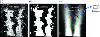


 Open access

