


1. Introduction
Over 20 % of the Earth’s surface can be characterized as hilly or mountainous terrain (e.g. Körner et al. Reference Körner, Hassan, Scholes and Ash2005). Although tall mountainous regions of the world garner substantial focus in meteorology (e.g. Bougeault et al. Reference Bougeault, Binder, Buzzi, Dirks, Kuettner, Houze, Smith, Steinacker and Volkert2001; Grubišić et al. Reference Grubišić2008; Houze et al. Reference Houze2017), the Earth’s hypsographic curve interestingly shows that most of Earth’s terrain is less than 1000 m in height (e.g. Lagrula Reference Lagrula1968; Cawood et al. Reference Cawood, Chowdhury, Mulder, Hawkesworth, Capitanio, Gunawardana and Nebel2022). Even in large-scale mountainous terrain, terrain height spectra demonstrate substantial variance at small scales (e.g. Young & Pielke Reference Young and Pielke1983). While today’s weather, air pollution and climate models can potentially resolve the larger-scale terrain features (e.g. mountains), the ability to resolve gentle small-scale hills currently remains beyond reach in larger-scale models. Due to the prevalence of small-scale hills, understanding their influence on turbulent flow is also essential for proper measurement interpretation, and for describing pollutant, aerosol and seed transport, and for predicting wind throw and wind energy availability (e.g. Finnigan et al. Reference Finnigan, Ayotte, Harman, Katul, Oldroyd, Patton, Poggi, Ross and Taylor2020).
Under neutrally stratified conditions, inviscid incompressible flow over a low symmetric obstacle produces a pressure minima occurring at the obstacle crest but does not generate any resistance (drag) because the pressure perturbation remains symmetric relative to the obstacle in the absence of any momentum stress (e.g. d’Alembert Reference d’Alembert1752; Calero Reference Calero2018). In laminar incompressible flow, the addition of finite viscosity ensures a thickening of the boundary layer (a greater separation of the streamlines) in a hill-like obstacle’s lee due to the spatially varying action of viscous drag which produces a pressure perturbation phase-shifted slightly downstream relative to the obstacle resulting in form drag (typically referred to as sheltering, e.g. Prandtl (Reference Prandtl1904)). Turbulent incompressible flows over hills also produce form drag through sheltering but the turbulent stresses dominate the smaller viscous stresses resulting in even larger pressure asymmetry relative to the hill shape producing even larger drag (e.g. Jackson & Hunt Reference Jackson and Hunt1975; Britter, Hunt & Richards Reference Britter, Hunt and Richards1981; Hunt, Leibovich & Richards Reference Hunt, Leibovich and Richards1988; Belcher, Newley & Hunt Reference Belcher, Newley and Hunt1993). Characteristics of the hill can alter the flow’s evolution over the obstacle, e.g. flow over steeper hills induces larger amplitude pressure perturbations and this obstacle-induced pressure perturbation can generate a sufficiently large near-surface adverse pressure-gradient on the hill’s lee that downward turbulent transport of momentum from aloft becomes insufficient to counter the adverse pressure-gradient producing flow separation; whether the flow separates or not dramatically alters the pressure field and hence the overall form drag felt by the outer flow (e.g. Taylor, Mason & Bradley Reference Taylor, Mason and Bradley1987; Finnigan et al. Reference Finnigan, Raupach, Bradley and Aldis1990; Wood & Mason Reference Wood and Mason1993; Athanassiadou & Castro Reference Athanassiadou and Castro2001). Because surface roughness alters the turbulence, variations in surface roughness also modulate flow responses to hills and the induced separation (e.g. Britter et al. Reference Britter, Hunt and Richards1981; Ayotte & Hughes Reference Ayotte and Hughes2004; Tamura, Okuno & Sugio Reference Tamura, Okuno and Sugio2007). Flow over two-dimensional (2D) versus three-dimensional (3D) hills (e.g. ridges versus isolated hills) also differs substantially because of the ability for flow over 3D hills to divert around the hill, which produces spanwise shear around the edges of and in the lee of the hill altering the turbulence and separation by generating additional instabilities and vortices (e.g. Mason & Sykes Reference Mason and Sykes1979; Hunt & Snyder Reference Hunt and Snyder1980; Mason & King Reference Mason and King1985; Arya & Gadiyaram Reference Arya and Gadiyaram1986; Gong & Ibbetson Reference Gong and Ibbetson1989; Ishihara, Hibi & Oikawa Reference Ishihara, Hibi and Oikawa1999; Liu et al. Reference Liu, Cao, Liu and Ishihara2019a , Reference Liu, Diao and Ishiharab , Reference Liu, Wang, Wang and Ishihara2020).
Because mountainous and hilly terrain compresses climate zones and creates small-scale habitat diversity, these regions support more than one quarter of the Earth’s terrestrial biodiversity (e.g. Körner et al. Reference Körner, Hassan, Scholes and Ash2005). Hilly terrain is therefore frequently forested. Finnigan & Belcher (Reference Finnigan and Belcher2004) demonstrated using linearized theory that because forests interact with the flow through pressure drag, forests on hills can shift the hill-induced pressure perturbation enough to induce separation at notably smaller slopes than expected over hills of similarly specified roughness. Finnigan & Belcher’s (Reference Finnigan and Belcher2004) theory also predicts that flow separation should depend on the distribution and density of the canopy elements, which Patton & Katul (Reference Patton and Katul2009) later confirmed. Researchers such as Wilson, Finnigan & Raupach (Reference Wilson, Finnigan and Raupach1998), Poggi et al. (Reference Poggi, Katul, Albertson and Ridolfi2007) and Ross (Reference Ross2008) discussed that within-canopy turbulence mixing length scales vary with position over sinusoidally repeating forested hills. When investigating turbulent flow over observed Amazonian terrain, Chen, Chamecki & Katul (Reference Chen, Chamecki and Katul2020) found separated flow even in the lee of small bumps, and Chamecki et al. (Reference Chamecki, Freire, Dias, Chen, Dias-Junior, Toledo Machado, Sörgel, Tsokankunku and de Araújo2020) and Chen & Chamecki (Reference Chen and Chamecki2023) showed that imbalances in above-canopy turbulent kinetic energy (TKE) budgets can result from upstream terrain influences. With the exception of Chamecki et al. (Reference Chamecki, Freire, Dias, Chen, Dias-Junior, Toledo Machado, Sörgel, Tsokankunku and de Araújo2020), Chen et al. (Reference Chen, Chamecki and Katul2020) and Chen & Chamecki (Reference Chen and Chamecki2023), much of this literature discussing turbulence over forested hills has focused on 2D sinusoidally repeating hills.
To our knowledge, Finnigan & Brunet (Reference Finnigan, Brunet, Coutts and Grace1995) represents the first effort describing within- and above-canopy turbulent flow over isolated forested hills, where they documented that above-canopy streamlines dip into the canopy at approximately one-third the way up the windward side of a 2D isolated hill that can eliminate (or even reverse) the inflection point in the mean velocity profile expected in canopy-flows (e.g. Raupach, Finnigan & Brunet Reference Raupach, Finnigan and Brunet1996; Finnigan, Shaw & Patton Reference Finnigan, Shaw and Patton2009); a phenomenon that has important implications for turbulence production at canopy-top. Neff & Meroney (Reference Neff and Meroney1998) found that canopy-gaps influence hill-induced fractional speed-up factors and flow separation. Through two-point correlation analysis, Dupont & Brunet (Reference Dupont and Brunet2008) noted that turbulence in the intermittent leeward separation zone is not correlated with canopy-top turbulence on the windward side of the hill. Grant et al. (Reference Grant, Ross, Gardiner and Mobbs2015) found key features predicted by Finnigan & Belcher’s (Reference Finnigan and Belcher2004) theory in their field measurements over an isolated forested ridge. For a given hill shape, Ma et al. (Reference Ma, Liu, Banerjee, Katul, Yi and Pardyjak2020) demonstrated that variation in a canopy’s morphology modulates the position, strength and depth of the leeward separation bubble. Similar to Wood (Reference Wood2000) who discussed flow over hills with unresolved roughness, Tolladay & Chemel (Reference Tolladay and Chemel2021) demonstrated resolution influences on key turbulence statistics in large-eddy simulation (LES) of flow over the same isolated forested ridge as that studied by Ma et al. (Reference Ma, Liu, Banerjee, Katul, Yi and Pardyjak2020). These efforts have enhanced the general understanding of the role tall vegetation plays in modulating turbulent flow over infinitely long isolated ridges; how canopies modulate turbulence over 3D hills remains understudied.
Towards understanding the role that hill shape and slope play in modulating turbulence, we analyse four LESs of turbulent flow over isolated forested hills. These four simulations include two each at two different hill slopes. For each hill slope, the simulations conducted include one targeting flow over an infinitely wide 2D hill and one over an axisymmetric 3D hill. In collaboration with the effort reported here, colleagues conducted a comprehensive WT experiment studying neutrally stratified turbulent over 3D forested hills (figure 1, Harman & Finnigan Reference Harman and Finnigan2018). The numerical simulations attempt to reproduce the physical WT simulations over axisymmetric 3D hills (Harman & Finnigan Reference Harman and Finnigan2018) and 2D hills.
A photograph of the forested isolated axisymmetric 3D steep ( $s_m =\,$
0.26) cosine hill surface in the wind tunnel (WT) (Harman & Finnigan Reference Harman and Finnigan2018).
$s_m =\,$
0.26) cosine hill surface in the wind tunnel (WT) (Harman & Finnigan Reference Harman and Finnigan2018).

The outline of this manuscript is as follows: § 2 discusses current theory describing turbulent flow over forested hills. Section 3 describes the simulations investigated. Section 4 outlines the techniques used to analyse the simulation data. Section 5 compares the simulation results against WT measurements from Harman & Finnigan (Reference Harman and Finnigan2018). Section 6 describes the mean flow and turbulence response to variations in hill shape and slope. Section 7 interrogates turbulence/mean-flow phase relationships at key heights above the surface towards advancing current theory, and § 8 summarizes the findings.
2. Current theory describing turbulent flow over forested hills
Current analytic theory of turbulent shear flow over low hills (e.g. Jackson & Hunt Reference Jackson and Hunt1975; Hunt et al. Reference Hunt, Leibovich and Richards1988; Belcher et al. Reference Belcher, Newley and Hunt1993) has provided an enduring and consistent framework for analysis and understanding of flow over low hills and even over steeper hills upwind of the separation region. The theory divides the flow into different layers, where the perturbations to the mean flow caused by the hill are governed by distinctly different dynamics. Separate solutions to the flow equations are found for each layer and then these are matched asymptotically between the layers. For hills of sufficiently low-slope to ignore flow separation, Hunt et al. (Reference Hunt, Leibovich and Richards1988) defined two main regions: (i) the outer region, where the response to the pressure field generated by flow over the hill is inviscid, and (ii) the inner region, where perturbations to the turbulent Reynolds stresses affect the perturbations to the mean flow. Each of these regions was further divided into two layers. The middle layer, of depth $h_m$
, is the lower part of the outer region through which flow responses are inviscid but rotational to accommodate shear in the approach flow. In the upper layer, extending from
$h_m$
, is the lower part of the outer region through which flow responses are inviscid but rotational to accommodate shear in the approach flow. In the upper layer, extending from $h_m$
to the top of the boundary layer, flow responses are irrotational and can be computed by potential theory. The inner region consists of the shear stress layer of depth
$h_m$
to the top of the boundary layer, flow responses are irrotational and can be computed by potential theory. The inner region consists of the shear stress layer of depth $h_i$
, and the thin inner surface layer, of depth
$h_i$
, and the thin inner surface layer, of depth $l_s$
, which allows formal matching with a surface boundary condition.
$l_s$
, which allows formal matching with a surface boundary condition.
Finnigan & Belcher (Reference Finnigan and Belcher2004) extended the analytic theory of Hunt et al. (Reference Hunt, Leibovich and Richards1988) to hills covered by tall plant canopies by replacing the thin inner surface layer by a deep plant canopy parameterized by linearized flow equations in the upper canopy but where the unavoidably nonlinear dynamics in the lower canopy were treated heuristically. Harman & Finnigan (Reference Harman and Finnigan2009, Reference Harman and Finnigan2013) further developed Finnigan & Belcher (Reference Finnigan and Belcher2004) to accommodate more realistic 2D hills, and then Harman & Finnigan (Reference Harman and Finnigan2021) extended the theory to 3D hills.
In all of these small perturbation theories, whether over hills covered by a rough surface or a tall canopy, identifying the depths of the inner shear stress layer, $h_i$
, and the middle layer,
$h_i$
, and the middle layer, $h_m$
, is critical to applying the theory. To derive the formula for
$h_m$
, is critical to applying the theory. To derive the formula for $h_m$
, Hunt et al. (Reference Hunt, Leibovich and Richards1988) assumed that the flow approaching the hill could be described by a logarithmic profile in equilibrium with the upstream surface while in the inner shear stress layer
$h_m$
, Hunt et al. (Reference Hunt, Leibovich and Richards1988) assumed that the flow approaching the hill could be described by a logarithmic profile in equilibrium with the upstream surface while in the inner shear stress layer $h_i$
, the interdependence of the perturbations to the turbulent shear stresses and the perturbations to the mean shear are assumed to obey the same mixing length flux-gradient relationship as in an equilibrium log law. Finnigan & Belcher (Reference Finnigan and Belcher2004) relies on the same formulae for
$h_i$
, the interdependence of the perturbations to the turbulent shear stresses and the perturbations to the mean shear are assumed to obey the same mixing length flux-gradient relationship as in an equilibrium log law. Finnigan & Belcher (Reference Finnigan and Belcher2004) relies on the same formulae for $h_m$
and
$h_m$
and $h_i$
as Hunt et al. (Reference Hunt, Leibovich and Richards1988).
$h_i$
as Hunt et al. (Reference Hunt, Leibovich and Richards1988).
The formulae for $h_m$
and
$h_m$
and $h_i$
assume the flow over the hill remains attached (i.e. no flow separation). Over steeper 2D hills and over 3D hills, this assumption breaks down. If the flow separates, streamlines that were following the surface contour upwind leave the surface and delineate the boundary of a separation bubble. Downwind of the separation point the scale of the largest turbulent eddies increases abruptly. In the attached flow the largest eddies are limited by the local distance to the surface but after separation the largest eddies span the bubble depth, which is typically
$h_i$
assume the flow over the hill remains attached (i.e. no flow separation). Over steeper 2D hills and over 3D hills, this assumption breaks down. If the flow separates, streamlines that were following the surface contour upwind leave the surface and delineate the boundary of a separation bubble. Downwind of the separation point the scale of the largest turbulent eddies increases abruptly. In the attached flow the largest eddies are limited by the local distance to the surface but after separation the largest eddies span the bubble depth, which is typically ${ {O}}(H)$
with
${ {O}}(H)$
with $H$
representing the hill height. While the streamlines approaching a 3D hill in its plane of lateral symmetry go over the hill-centreline, streamlines to either side are deflected forming space curves whose principal normals intersect the hill surface at right angles (Finnigan Reference Finnigan2024).
$H$
representing the hill height. While the streamlines approaching a 3D hill in its plane of lateral symmetry go over the hill-centreline, streamlines to either side are deflected forming space curves whose principal normals intersect the hill surface at right angles (Finnigan Reference Finnigan2024).
As fluid parcels above the canopy advect over the hill, changes to the Reynolds stresses reflect the competing effects of two processes. First, the existing eddies are stretched and rotated by the mean flow as they follow the mean streamlines. Second, nonlinear interactions between the eddies will tend to equalize $T\!K\!E$
between their orthogonal components
$T\!K\!E$
between their orthogonal components $u^{\prime}$
,
$u^{\prime}$
, $v^{\prime}$
and
$v^{\prime}$
and $w^{\prime}$
, and to transfer TKE to finer scale eddies where it is ultimately dissipated to heat through the action of viscosity. These effects are represented formally in the conservation equations for the turbulent normal and shear stresses,
$w^{\prime}$
, and to transfer TKE to finer scale eddies where it is ultimately dissipated to heat through the action of viscosity. These effects are represented formally in the conservation equations for the turbulent normal and shear stresses, $\langle u'^2 \rangle$
,
$\langle u'^2 \rangle$
, $\langle v'^2 \rangle$
,
$\langle v'^2 \rangle$
, $\langle w'^2 \rangle$
,
$\langle w'^2 \rangle$
, $\langle u'w' \rangle$
,
$\langle u'w' \rangle$
, $\langle v'w' \rangle$
and
$\langle v'w' \rangle$
and $T\!K\!E$
, where
$T\!K\!E$
, where $T\!K\!E = (\langle u'^2 \rangle + \langle v'^2 \rangle + \langle w'^2 \rangle )/2$
. In these equations, the so-called production terms describe the transfer of kinetic energy from the mean flow to the larger energy-containing eddies of the turbulence while the turbulent diffusion and pressure-strain terms describe the nonlinear interactions between these eddies, which break them down and destroy their coherence. These nonlinear interactions determine
$T\!K\!E = (\langle u'^2 \rangle + \langle v'^2 \rangle + \langle w'^2 \rangle )/2$
. In these equations, the so-called production terms describe the transfer of kinetic energy from the mean flow to the larger energy-containing eddies of the turbulence while the turbulent diffusion and pressure-strain terms describe the nonlinear interactions between these eddies, which break them down and destroy their coherence. These nonlinear interactions determine $\tau$
, the time over which the large eddies remain coherent enough to receive energy directly from the mean flow. Here
$\tau$
, the time over which the large eddies remain coherent enough to receive energy directly from the mean flow. Here $\tau$
can be taken as
$\tau$
can be taken as $\tau \sim T\!K\!E/\epsilon$
, where
$\tau \sim T\!K\!E/\epsilon$
, where $\epsilon$
is the rate of viscous dissipation of TKE. This definition is strictly only applicable to equilibrium situations, where the rate of viscous dissipation is in balance with the transfer of kinetic energy from the mean flow to the turbulence, but we will assume that is also indicative of the rate at which these large eddies lose their coherence as they interact with each other during their passage over the hill.
$\epsilon$
is the rate of viscous dissipation of TKE. This definition is strictly only applicable to equilibrium situations, where the rate of viscous dissipation is in balance with the transfer of kinetic energy from the mean flow to the turbulence, but we will assume that is also indicative of the rate at which these large eddies lose their coherence as they interact with each other during their passage over the hill.
In regions where the time scale of hill-induced changes in the mean flow is small compared with $\tau$
(i.e. in the so-called rapid distortion regimes), the turbulent stresses will reflect their recent history of straining and rotation by the mean flow and Hunt et al. (Reference Hunt, Leibovich and Richards1988) assumes that this will be the case in the outer region in general and in the middle layer in particular. In regions where mean flow changes are slow compared with
$\tau$
(i.e. in the so-called rapid distortion regimes), the turbulent stresses will reflect their recent history of straining and rotation by the mean flow and Hunt et al. (Reference Hunt, Leibovich and Richards1988) assumes that this will be the case in the outer region in general and in the middle layer in particular. In regions where mean flow changes are slow compared with $\tau$
, the turbulence will approach a state of local equilibrium between the rate of straining by the mean flow and the resulting Reynolds stresses so that their relationship can be described by an eddy viscosity. Current theory assumes that we should observe this behaviour in the inner shear stress layer,
$\tau$
, the turbulence will approach a state of local equilibrium between the rate of straining by the mean flow and the resulting Reynolds stresses so that their relationship can be described by an eddy viscosity. Current theory assumes that we should observe this behaviour in the inner shear stress layer, $z \lt h_i$
.
$z \lt h_i$
.
Beneath the inner layer and above the ground surface lies the canopy layer, which introduces additional length scales ( $L_c$
and
$L_c$
and $h_c$
), through the addition of canopy drag and the no-slip condition at the surface. In the canopy, turbulent stresses are complicated by wake production,
$h_c$
), through the addition of canopy drag and the no-slip condition at the surface. In the canopy, turbulent stresses are complicated by wake production, $W_p$
, i.e. the production of turbulent eddies at scales defined by the canopy elements and associated short-circuiting of the inertial energy cascade (Finnigan Reference Finnigan2000; Shaw & Patton Reference Shaw and Patton2003). In addition, viscous dissipation increases by the work performed by the turbulence against the viscous drag of the canopy elements (Ayotte, Finnigan & Raupach Reference Ayotte, Finnigan and Raupach1999; Shaw & Patton Reference Shaw and Patton2003). For dense canopies (
$W_p$
, i.e. the production of turbulent eddies at scales defined by the canopy elements and associated short-circuiting of the inertial energy cascade (Finnigan Reference Finnigan2000; Shaw & Patton Reference Shaw and Patton2003). In addition, viscous dissipation increases by the work performed by the turbulence against the viscous drag of the canopy elements (Ayotte, Finnigan & Raupach Reference Ayotte, Finnigan and Raupach1999; Shaw & Patton Reference Shaw and Patton2003). For dense canopies ( $h_c/L_c \gt 1$
), canopy drag eliminates the importance for the flow dynamics of shear stress at the underlying surface but at the same time ensures strong vertical gradients in turbulent stresses. Finally, behind the hill crest, the strong adverse pressure gradient can cause reversed flow and separation, which introduces the hill height
$h_c/L_c \gt 1$
), canopy drag eliminates the importance for the flow dynamics of shear stress at the underlying surface but at the same time ensures strong vertical gradients in turbulent stresses. Finally, behind the hill crest, the strong adverse pressure gradient can cause reversed flow and separation, which introduces the hill height $H$
as an additional length scale affecting the turbulence.
$H$
as an additional length scale affecting the turbulence.
3. Simulation description and configuration
Numerical models of turbulent flow over forested hills take many forms that each provide value with varying levels of accuracy and cost (see recent review by Finnigan et al. (Reference Finnigan, Ayotte, Harman, Katul, Oldroyd, Patton, Poggi, Ross and Taylor2020)). Analytical models provide extremely timely solutions, but typically linearize the nonlinear equations that describe turbulent flow (e.g. Finnigan & Belcher Reference Finnigan and Belcher2004; Poggi et al. Reference Poggi, Katul, Finnigan and Belcher2008; Harman & Finnigan Reference Harman and Finnigan2009, Reference Harman and Finnigan2013). Reynolds-averaged Navier–Stokes models solve the full nonlinear equations but averaged over space and time such that the influence of turbulence is fully parameterized (e.g. Wilson et al. Reference Wilson, Finnigan and Raupach1998; Katul & Chang Reference Katul and Chang1999; Ross & Vosper Reference Ross and Vosper2005, among others). Similar to Reynolds-averaged Navier–Stokes, LES also solves the full nonlinear equations but relies on relatively isotropic grids and only spatially averages (or filters) the equations at scales smaller than the grid resolution, such that the largest scales of turbulence (i.e. those performing most of the transport) are resolved by the grid and only the smallest scales of turbulence (which primarily act to dissipate energy) must be parameterized (e.g. Moeng & Sullivan Reference Moeng and Sullivan2015). Although it is computationally expensive, LES has become a close counterpart to field and laboratory experiments over the past 30 plus years because of its ability to accurately simulate the time-evolving and spatially evolving response of turbulence to varying forcing over complex surfaces (e.g. Wood Reference Wood2000; Patton & Katul Reference Patton and Katul2009; Sullivan, McWilliams & Patton Reference Sullivan, McWilliams and Patton2014; Chamecki et al. Reference Chamecki, Freire, Dias, Chen, Dias-Junior, Toledo Machado, Sörgel, Tsokankunku and de Araújo2020).
In our LES, the governing equations describe 3D time-dependent turbulent winds in a dry incompressible Boussinesq atmospheric boundary layer, including (i) three transport equations for momentum $\rho {\boldsymbol{u}}$
, (ii) a transport equation for a conserved scalar variable, (iii) a discrete Poisson equation for a pressure variable
$\rho {\boldsymbol{u}}$
, (ii) a transport equation for a conserved scalar variable, (iii) a discrete Poisson equation for a pressure variable $p$
to enforce incompressibility and (iv) closure expressions for subgrid-scale (SGS) variables, e.g. an equation for SGS TKE
$p$
to enforce incompressibility and (iv) closure expressions for subgrid-scale (SGS) variables, e.g. an equation for SGS TKE $e$
(see Sullivan et al. Reference Sullivan, McWilliams and Patton2014). The physical processes included in the LES boundary-layer equations include, temporal time tendencies, advection, pressure gradients, divergence of SGS fluxes, buoyancy, resolved turbulence, and in the case of the SGS
$e$
(see Sullivan et al. Reference Sullivan, McWilliams and Patton2014). The physical processes included in the LES boundary-layer equations include, temporal time tendencies, advection, pressure gradients, divergence of SGS fluxes, buoyancy, resolved turbulence, and in the case of the SGS $e$
equation also diffusion and dissipation.
$e$
equation also diffusion and dissipation.
Explicit spatial filtering of the momentum equations in the presence of vegetative-canopy elements generates terms representing canopy-induced pressure and viscous drag (Finnigan & Shaw Reference Finnigan and Shaw2008) which are parameterized using a time-dependent and local velocity-squared type drag law, e.g.
 \begin{equation} F_c = -\, c_d\,a\,|\boldsymbol{u}|\,\boldsymbol{u}, \end{equation}
where, $a$
is the canopy’s frontal area density and
$a$
is the canopy’s frontal area density and $c_d$
is a drag coefficient describing the canopy’s efficiency at absorbing momentum. Dissipation in the SGS energy equation is also augmented by the work SGS motions perform against the canopy-induced form drag. See Shaw & Patton (Reference Shaw and Patton2003), Patton & Katul (Reference Patton and Katul2009) and Patton et al. (Reference Patton, Sullivan, Shaw, Finnigan and Weil2016) for further details of the canopy representation in the LES.
$c_d$
is a drag coefficient describing the canopy’s efficiency at absorbing momentum. Dissipation in the SGS energy equation is also augmented by the work SGS motions perform against the canopy-induced form drag. See Shaw & Patton (Reference Shaw and Patton2003), Patton & Katul (Reference Patton and Katul2009) and Patton et al. (Reference Patton, Sullivan, Shaw, Finnigan and Weil2016) for further details of the canopy representation in the LES.
By applying a transformation to the physical space coordinates $(x,y,z)$
that maps them onto flat computational coordinates
$(x,y,z)$
that maps them onto flat computational coordinates $(\xi ,\eta ,\zeta )$
, Sullivan et al. (Reference Sullivan, McWilliams and Patton2014) adapted our flat LES (Sullivan & Patton Reference Sullivan and Patton2011) to a situation with a 3D time-evolving lower boundary shape
$(\xi ,\eta ,\zeta )$
, Sullivan et al. (Reference Sullivan, McWilliams and Patton2014) adapted our flat LES (Sullivan & Patton Reference Sullivan and Patton2011) to a situation with a 3D time-evolving lower boundary shape $h = h(x,y,t)$
. The current simulations use this same framework, but impose a time-independent surface, e.g.
$h = h(x,y,t)$
. The current simulations use this same framework, but impose a time-independent surface, e.g. $h = h(x,y)$
where the maximum hill slope
$h = h(x,y)$
where the maximum hill slope $s_m = \text {max}( {\partial h}/{\partial x})$
. Of importance is that we transform the coordinates, not the flow variables. Therefore, horizontal velocity components (
$s_m = \text {max}( {\partial h}/{\partial x})$
. Of importance is that we transform the coordinates, not the flow variables. Therefore, horizontal velocity components ( $u$
,
$u$
, $v$
) are defined in a right-handed Cartesian coordinate system parallel to the flat surface surrounding each hill (with
$v$
) are defined in a right-handed Cartesian coordinate system parallel to the flat surface surrounding each hill (with $u$
aligned with the imposed pressure gradient force in the
$u$
aligned with the imposed pressure gradient force in the $+x$
direction, and
$+x$
direction, and $v$
positive to the left of the imposed pressure gradient force in the
$v$
positive to the left of the imposed pressure gradient force in the $+y$
direction), and vertical velocity (
$+y$
direction), and vertical velocity ( $w$
) is defined positive upward from the underlying flat surface (the
$w$
) is defined positive upward from the underlying flat surface (the $+z$
direction) aligned opposite to the gravitational force (although the flow under consideration is neutrally stratified, so gravitational forces are ignored).
$+z$
direction) aligned opposite to the gravitational force (although the flow under consideration is neutrally stratified, so gravitational forces are ignored).
The simulations discretize a 4096 $\times$
2048
$\times$
2048 $\times$
512 m
$\times$
512 m $^3$
domain using 2048
$^3$
domain using 2048 $\times$
1024
$\times$
1024 $\times$
256 grid points. The computational mesh in physical space is surface following and non-orthogonal. Vertical grid lines are held fixed at a particular
$\times$
256 grid points. The computational mesh in physical space is surface following and non-orthogonal. Vertical grid lines are held fixed at a particular $(x,y)$
location but the horizontal grid lines undergo vertical translation according to the vertical variation of the underlying surface. While the grid resolution in the horizontal directions is fixed for all horizontal locations, the vertical grid is refined near the surface to resolve near-surface/canopy processes and is then algebraically stretched above the canopy to push the upper boundary far above the hill to minimize any influence of the upper boundary on the hill-induced pressure field. Care is taken to ensure that every grid volume uses an aspect ratio no larger than
$(x,y)$
location but the horizontal grid lines undergo vertical translation according to the vertical variation of the underlying surface. While the grid resolution in the horizontal directions is fixed for all horizontal locations, the vertical grid is refined near the surface to resolve near-surface/canopy processes and is then algebraically stretched above the canopy to push the upper boundary far above the hill to minimize any influence of the upper boundary on the hill-induced pressure field. Care is taken to ensure that every grid volume uses an aspect ratio no larger than $5:1$
attempting to reasonably satisfy isotropy assumptions used to close the equations in the SGS model.
$5:1$
attempting to reasonably satisfy isotropy assumptions used to close the equations in the SGS model.
Example of the horizontal domains used and the idealized cosine-shaped 2D and 3D hills. Panel (b) reflects the axisymmetric case with $L = L_y = L_x$
. The blue line spanning the domain at
$L = L_y = L_x$
. The blue line spanning the domain at $x$
= 1024 m depicts the downwind boundary of the horizontally homogeneous periodic region, while the green line spanning the domain at
$x$
= 1024 m depicts the downwind boundary of the horizontally homogeneous periodic region, while the green line spanning the domain at $x \sim$
3892 m depicts the beginning of the fringe region where the solutions begin to be nudged back to those at the downwind edge of the upwind periodic region starting at the green line located at
$x \sim$
3892 m depicts the beginning of the fringe region where the solutions begin to be nudged back to those at the downwind edge of the upwind periodic region starting at the green line located at $x \sim$
820 m. Periodic boundary conditions are imposed in the
$x \sim$
820 m. Periodic boundary conditions are imposed in the $y$
-direction. The vertical domain extends up to 512 m.
$y$
-direction. The vertical domain extends up to 512 m.

Spatial differencing is pseudospectral in the horizontal computational directions $(\xi , \eta )$
and is second-order finite difference in
$(\xi , \eta )$
and is second-order finite difference in $\zeta$
. Time stepping uses a low-storage third-order Runge–Kutta scheme, and the time step
$\zeta$
. Time stepping uses a low-storage third-order Runge–Kutta scheme, and the time step $\delta t$
is picked dynamically based on a fixed Courant–Fredrichs–Lewy number.
$\delta t$
is picked dynamically based on a fixed Courant–Fredrichs–Lewy number.
An important development for this effort involves implementing a turbulent inflow fringe (or precursor) method which is compatible with our pseudospectral spatial differencing and third-order Runge–Kutta time differencing (Schlatter, Adams & Kleiser Reference Schlatter, Adams and Kleiser2005; Munters, Meneveau & Meyers Reference Munters, Meneveau and Meyers2016) to enable simulation of flow over isolated 2D and 3D hills. The strategy involves simulating two interconnected periodic domains, where the flow in the upwind domain is periodic and representative of flow over an infinitely long horizontally homogeneous forested surface. The outflow of that upwind domain serves as inflow for the downwind domain containing the hill. In the second domain at the boundary far downstream from the hill, nudging terms are applied over the downwind-most 102 grid points (from grid points 1946–2048) to force the exit flow of the larger downwind domain to match the flow exiting the upstream region (note that 102 grid points is 20 % of the upwind domain). Hence both domains use periodic boundary conditions in the $x$
direction, but the flow impinging on the hill is unaware of any upstream hills. It is important to note two things: (i) the size of the upstream inflow domain dictates the largest scales of motion impinging on the hill located in the downstream domain, and (ii) the chosen fringe strategy used in these simulations was developed prior to and differs from the two-domain strategy discussed in Sullivan et al. (Reference Sullivan, McWilliams, Weil, Patton and Fernando2020, Reference Sullivan, McWilliams, Weil, Patton and Fernando2021) that ensures decoupling of inflow conditions from any slight imperfections in the spectral tapering (e.g. Inoue, Matheou & Teixeira Reference Inoue, Matheou and Teixeira2014) and which enables inclusion of Coriolis and buoyancy forces. (For these reasons, we recommend using the technique described by Sullivan et al. (Reference Sullivan, McWilliams, Weil, Patton and Fernando2020, Reference Sullivan, McWilliams, Weil, Patton and Fernando2021) for future studies.) Figure 2 shows the total extent of the horizontal domain for the two steeper hill configurations (
$x$
direction, but the flow impinging on the hill is unaware of any upstream hills. It is important to note two things: (i) the size of the upstream inflow domain dictates the largest scales of motion impinging on the hill located in the downstream domain, and (ii) the chosen fringe strategy used in these simulations was developed prior to and differs from the two-domain strategy discussed in Sullivan et al. (Reference Sullivan, McWilliams, Weil, Patton and Fernando2020, Reference Sullivan, McWilliams, Weil, Patton and Fernando2021) that ensures decoupling of inflow conditions from any slight imperfections in the spectral tapering (e.g. Inoue, Matheou & Teixeira Reference Inoue, Matheou and Teixeira2014) and which enables inclusion of Coriolis and buoyancy forces. (For these reasons, we recommend using the technique described by Sullivan et al. (Reference Sullivan, McWilliams, Weil, Patton and Fernando2020, Reference Sullivan, McWilliams, Weil, Patton and Fernando2021) for future studies.) Figure 2 shows the total extent of the horizontal domain for the two steeper hill configurations ( $s_m =$
0.26). The blue lines in figure 2 mark the boundaries where periodicity in the
$s_m =$
0.26). The blue lines in figure 2 mark the boundaries where periodicity in the $x$
direction is enforced. The green lines in figure 2 mark the starting point of the region where the nudging algorithm operates, with the left-hand side showing the horizontally homogeneous region used to nudge the downstream flow back to horizontally homogeneous flow that is unaware of the hill and the right-hand side showing the region that is nudged back to the upwind conditions. Periodic boundary conditions are imposed in the lateral (
$x$
direction is enforced. The green lines in figure 2 mark the starting point of the region where the nudging algorithm operates, with the left-hand side showing the horizontally homogeneous region used to nudge the downstream flow back to horizontally homogeneous flow that is unaware of the hill and the right-hand side showing the region that is nudged back to the upwind conditions. Periodic boundary conditions are imposed in the lateral ( $y$
) direction, the upper boundary is a frictionless rigid lid, and the lower boundary beneath the trees uses a rough-wall neutrally stratified drag law with a surface roughness length
$y$
) direction, the upper boundary is a frictionless rigid lid, and the lower boundary beneath the trees uses a rough-wall neutrally stratified drag law with a surface roughness length $z_{\circ } = 1\times 10^{-3}$
m.
$z_{\circ } = 1\times 10^{-3}$
m.
To minimize the computational expense, all the simulations are generated by first integrating a smaller $512\times 512\times 256$
grid point flat-domain simulation out in time using periodic horizontal boundary conditions until the initially laminar flow develops from divergence free random fluctuations into 3D turbulence that is in equilibrium with the imposed pressure gradient. Upon reaching equilibrium, a restart volume is saved. This volume is then mirrored one time in the lateral (
$512\times 512\times 256$
grid point flat-domain simulation out in time using periodic horizontal boundary conditions until the initially laminar flow develops from divergence free random fluctuations into 3D turbulence that is in equilibrium with the imposed pressure gradient. Upon reaching equilibrium, a restart volume is saved. This volume is then mirrored one time in the lateral ( $y$
) and four times in the downwind (
$y$
) and four times in the downwind ( $x$
) directions to create a fully turbulent initial condition for the full large-domain simulations. The code is then reconfigured to: (i) restart from this larger volume, and (ii) run using the precursor inflow boundary condition in the along-wind (
$x$
) directions to create a fully turbulent initial condition for the full large-domain simulations. The code is then reconfigured to: (i) restart from this larger volume, and (ii) run using the precursor inflow boundary condition in the along-wind ( $x$
) direction. Upon restart, a hill is gradually grown into the downwind portion of the domain over a period of 400 s. Averaging begins after integrating forward in this configuration for approximately one large-eddy turnover time to allow the turbulence to evolve into the new configuration. Running on 2048 CPUs on an HPE SGI ICE XA system (Computational and Information Systems Laboratory 2019), the (2D; 3D)-hill simulations required approximately (77; 366) wallclock hours, respectively.
$x$
) direction. Upon restart, a hill is gradually grown into the downwind portion of the domain over a period of 400 s. Averaging begins after integrating forward in this configuration for approximately one large-eddy turnover time to allow the turbulence to evolve into the new configuration. Running on 2048 CPUs on an HPE SGI ICE XA system (Computational and Information Systems Laboratory 2019), the (2D; 3D)-hill simulations required approximately (77; 366) wallclock hours, respectively.
As in the WT measurements (Harman & Finnigan Reference Harman and Finnigan2018), the flow is neutrally stratified (no buoyancy) and Coriolis forces are ignored. The hills are of cosine shape,
 \begin{align} \quad \quad \quad \quad h(x,y) &= H \, {\textrm{cos}}^2\left (\frac {\pi \; \widehat {x}}{4}\right ) &\text{when} \quad |\,\widehat {x}\,| \le 2, \quad \quad \quad \quad \end{align}
 \begin{align} \quad \quad \quad \quad h(x,y) &= 0 &\text{when} \quad |\,\widehat {x}\,| \gt 2, \quad \quad \quad \quad \end{align}
where, $H$
is the hill height. In the 2D-hill case,
$H$
is the hill height. In the 2D-hill case,
 \begin{equation} \widehat {x} = \frac {x - x_{\circ }}{L_x} ,\end{equation}
and, in the 3D-hill case,
 \begin{equation} \widehat {x} = \left [ \left (\frac {x - x_{\circ }}{L_x}\right )^2 + \left (\frac {y - y_{\circ }}{L_y}\right )^2 \right ]^{\frac {1}{2}}\!, \end{equation}
where $L_x$
and
$L_x$
and $L_y$
are the hill lengths at the hill half-height in the
$L_y$
are the hill lengths at the hill half-height in the $x$
and
$x$
and $y$
directions, respectively, and (
$y$
directions, respectively, and ( $x_{\circ }, y_{\circ }$
) represent the physical location of the hill crest. In the axisymmetric 3D hill simulations,
$x_{\circ }, y_{\circ }$
) represent the physical location of the hill crest. In the axisymmetric 3D hill simulations, $L_x = L_y = L$
. Variations in hill steepness are generated by keeping
$L_x = L_y = L$
. Variations in hill steepness are generated by keeping $H$
fixed and varying
$H$
fixed and varying $L$
. Scaling up the WT hills by a factor of 256,
$L$
. Scaling up the WT hills by a factor of 256, $H = 12.8$
m for all cases; see table 1 for the matching values of
$H = 12.8$
m for all cases; see table 1 for the matching values of $L$
. Figure 3 shows examples of the surfaces investigated with the LES. The
$L$
. Figure 3 shows examples of the surfaces investigated with the LES. The $x$
,
$x$
, $y$
grid lines follow this surface and algebraically relax back to horizontal grid lines parallel to the upwind flat surface at approximately the domain half-height (see (4) in Sullivan et al. (Reference Sullivan, McWilliams and Patton2014), where we use
$y$
grid lines follow this surface and algebraically relax back to horizontal grid lines parallel to the upwind flat surface at approximately the domain half-height (see (4) in Sullivan et al. (Reference Sullivan, McWilliams and Patton2014), where we use $\varpi = 3$
).
$\varpi = 3$
).
Bulk parameters from each of the four simulations. Here $s_m$
is the maximum hill slope (
$s_m$
is the maximum hill slope ( $\text {max}( {\partial h}/{\partial x})$
),
$\text {max}( {\partial h}/{\partial x})$
), $L$
is the length of the hill (m) in the streamwise direction
$L$
is the length of the hill (m) in the streamwise direction $x$
at half the hill height (so the total hill length is 4L),
$x$
at half the hill height (so the total hill length is 4L), $u_*$
is the friction velocity (m s
$u_*$
is the friction velocity (m s $^{-1}$
) evaluated at
$^{-1}$
) evaluated at $x = -4L$
and
$x = -4L$
and $z = h_c$
(consistent with
$z = h_c$
(consistent with $u_*$
observed in the WT; when averaged over the entire upwind periodic domain,
$u_*$
observed in the WT; when averaged over the entire upwind periodic domain, $u_* = 0.42$
m s
$u_* = 0.42$
m s $^{-1}$
for all cases). Here
$^{-1}$
for all cases). Here $F_p = - \int _{-2L}^{2L}\langle p \rangle h_x\,{\rm d}x$
is the streamwise surface pressure drag integrated over the hill (e.g. the hill-induced pressure force on the air) normalized by
$F_p = - \int _{-2L}^{2L}\langle p \rangle h_x\,{\rm d}x$
is the streamwise surface pressure drag integrated over the hill (e.g. the hill-induced pressure force on the air) normalized by $u_*^2$
, where
$u_*^2$
, where $h_x = {\partial h}/{\partial x}$
is the
$h_x = {\partial h}/{\partial x}$
is the $x$
-varying hill slope),
$x$
-varying hill slope), $F_c = - \,c_d\,a \int _{-2L}^{2L}\int _{0}^{h_c} \langle |u_i| u \rangle \,{\rm d}z\,{\rm d}x$
is the hill- and canopy-integrated drag induced by the canopy in the streamwise direction and
$F_c = - \,c_d\,a \int _{-2L}^{2L}\int _{0}^{h_c} \langle |u_i| u \rangle \,{\rm d}z\,{\rm d}x$
is the hill- and canopy-integrated drag induced by the canopy in the streamwise direction and $F_{\tau } = \int _{-2L}^{2L}\langle u'w' \rangle \,{\rm d}x$
is the hill-integrated streamwise surface stress; the total drag felt by the flow over the hill
$F_{\tau } = \int _{-2L}^{2L}\langle u'w' \rangle \,{\rm d}x$
is the hill-integrated streamwise surface stress; the total drag felt by the flow over the hill $F_T = F_p + F_c + F_{\tau }$
. Here max
$F_T = F_p + F_c + F_{\tau }$
. Here max $(\Delta u/u_b)_{ h_c}$
, max
$(\Delta u/u_b)_{ h_c}$
, max $(\Delta \sigma _{\!u}/\sigma _{u_b})_{ h_c}$
, max
$(\Delta \sigma _{\!u}/\sigma _{u_b})_{ h_c}$
, max $(\Delta \sigma _{\!w}/\sigma _{w_b})_{ h_c}$
and max
$(\Delta \sigma _{\!w}/\sigma _{w_b})_{ h_c}$
and max $(\Delta uw/uw_b)_{ h_c}$
are the maximum hill- and canopy-induced speedup, standard deviation of streamwise and vertical velocity, and vertical flux of streamwise momentum increase at canopy top along hill centreline, respectively, where
$(\Delta uw/uw_b)_{ h_c}$
are the maximum hill- and canopy-induced speedup, standard deviation of streamwise and vertical velocity, and vertical flux of streamwise momentum increase at canopy top along hill centreline, respectively, where $\Delta u/u_b = [(\langle u \rangle - \langle u \rangle _{b}) / \langle u \rangle _{b}]$
,
$\Delta u/u_b = [(\langle u \rangle - \langle u \rangle _{b}) / \langle u \rangle _{b}]$
, $\Delta \sigma _{u}/\sigma _{u_b} = [(\sigma _u - \sigma _{u_{b}}) / \sigma _{u_{b}}]$
,
$\Delta \sigma _{u}/\sigma _{u_b} = [(\sigma _u - \sigma _{u_{b}}) / \sigma _{u_{b}}]$
, $\Delta \sigma _w/\sigma _{w_{b}} = [(\sigma _w - \sigma _{w_{b}}) / \sigma _{w_{b}}]$
and
$\Delta \sigma _w/\sigma _{w_{b}} = [(\sigma _w - \sigma _{w_{b}}) / \sigma _{w_{b}}]$
and $\Delta uw/uw_b = [(\langle u'w' \rangle - \langle u'w' \rangle _{b}) / \langle u'w' \rangle _{b}]$
evaluated at a height of
$\Delta uw/uw_b = [(\langle u'w' \rangle - \langle u'w' \rangle _{b}) / \langle u'w' \rangle _{b}]$
evaluated at a height of $h_c$
above the local surface
$h_c$
above the local surface $h$
, the notation
$h$
, the notation $_{b}$
refers to a reference value upwind of the hill (Appendix A) and the adjacent values in square brackets reflects the
$_{b}$
refers to a reference value upwind of the hill (Appendix A) and the adjacent values in square brackets reflects the $x/L$
location where the maximum canopy-top value is found.
$x/L$
location where the maximum canopy-top value is found.

The canopy parameters are derived directly from measurements of the rods used in the WT experiments (Harman & Finnigan Reference Harman and Finnigan2018). In the WT, the rods are 15 mm tall, 5 mm in diameter ( $d_r$
), and are spaced at 12.5 mm intervals in the
$d_r$
), and are spaced at 12.5 mm intervals in the $x$
direction and 25 mm in the
$x$
direction and 25 mm in the $y$
direction. Hence, the number of rods per unit area
$y$
direction. Hence, the number of rods per unit area $n_r$
= 3200 m
$n_r$
= 3200 m $^{-2}$
and the rods have a frontal area density
$^{-2}$
and the rods have a frontal area density $a = n_r \times r_d =$
16 m
$a = n_r \times r_d =$
16 m $^2$
m
$^2$
m $^{-3}$
that is constant with height. Fitting the WT observed profiles with the rods installed on flat terrain (Harman & Finnigan Reference Harman and Finnigan2018, figure 2
a) to the Harman & Finnigan (Reference Harman and Finnigan2007) roughness sublayer (RSL) theory reveals that the rods have an effective canopy length scale
$^{-3}$
that is constant with height. Fitting the WT observed profiles with the rods installed on flat terrain (Harman & Finnigan Reference Harman and Finnigan2018, figure 2
a) to the Harman & Finnigan (Reference Harman and Finnigan2007) roughness sublayer (RSL) theory reveals that the rods have an effective canopy length scale $L_c = (c_d\,a)^{-1}$
= 110 mm. Therefore, the drag coefficient
$L_c = (c_d\,a)^{-1}$
= 110 mm. Therefore, the drag coefficient $c_d$
of the rods is 0.57. In the numerical simulations, these rod parameters are applied to a canopy of height
$c_d$
of the rods is 0.57. In the numerical simulations, these rod parameters are applied to a canopy of height $h_c$
= 3.84 m resolved by nine grid points on the flat portion of the domain and by 10 grid points at the hill crest due to the terrain following coordinate system. To mimic the WT experiments, the canopy is prescribed to be horizontally homogeneous for all four simulations. Figure 1 shows an image of the WT configuration with the steep-sloped (
$h_c$
= 3.84 m resolved by nine grid points on the flat portion of the domain and by 10 grid points at the hill crest due to the terrain following coordinate system. To mimic the WT experiments, the canopy is prescribed to be horizontally homogeneous for all four simulations. Figure 1 shows an image of the WT configuration with the steep-sloped ( $s_m =$
0.26) axisymmetric canopy-covered hill installed.
$s_m =$
0.26) axisymmetric canopy-covered hill installed.
A zoomed presentation of the 2D (a) and 3D-axisymmetric (b) cosine hills interrogated. In (a), $L = L_x$
and
$L = L_x$
and $L_y$
is not defined, and in (b)
$L_y$
is not defined, and in (b) $L = L_x = L_y$
.
$L = L_x = L_y$
. $H$
is the hill height (3.2). The green surface depicts canopy top
$H$
is the hill height (3.2). The green surface depicts canopy top $h_c$
.
$h_c$
.

To classify the current simulations within the context of previous work, we first turn to the Hunt et al. (Reference Hunt, Leibovich and Richards1988) and Finnigan & Belcher (Reference Finnigan and Belcher2004) theories discussed in § 2. In both theories, the middle layer depth ( $h_m$
) is defined as
$h_m$
) is defined as $h_m \sim L\,[\text{ln}(h_m / z_{\circ })]^{{1}/{2}}$
, and the inner layer depth (
$h_m \sim L\,[\text{ln}(h_m / z_{\circ })]^{{1}/{2}}$
, and the inner layer depth ( $h_i$
) is defined as
$h_i$
) is defined as $h_i \sim 2\,L\,\kappa ^2 / \text{ln}(h_i / z_{\circ })$
, where
$h_i \sim 2\,L\,\kappa ^2 / \text{ln}(h_i / z_{\circ })$
, where $\kappa$
is von Kármán’s constant. However, calculating
$\kappa$
is von Kármán’s constant. However, calculating $h_i$
and
$h_i$
and $h_m$
using these formulations can lead to physically implausible values over surfaces covered with tall roughness, i.e.
$h_m$
using these formulations can lead to physically implausible values over surfaces covered with tall roughness, i.e. $h_i$
can end up being found at heights within the canopy of roughness elements (Finnigan et al. Reference Finnigan, Raupach, Bradley and Aldis1990). Therefore, Appendix B derives new formulae for
$h_i$
can end up being found at heights within the canopy of roughness elements (Finnigan et al. Reference Finnigan, Raupach, Bradley and Aldis1990). Therefore, Appendix B derives new formulae for $h_i$
and
$h_i$
and $h_m$
incorporating changes to the logarithmic mean velocity profile and the accompanying flux-gradient relationship which occur over a tall plant canopy (Harman & Finnigan Reference Harman and Finnigan2007, Reference Harman and Finnigan2008); labelled
$h_m$
incorporating changes to the logarithmic mean velocity profile and the accompanying flux-gradient relationship which occur over a tall plant canopy (Harman & Finnigan Reference Harman and Finnigan2007, Reference Harman and Finnigan2008); labelled $\widehat {h_m}$
and
$\widehat {h_m}$
and $\widehat {h_i}$
using similar notation to Harman & Finnigan (Reference Harman and Finnigan2007, Reference Harman and Finnigan2008). For the configurations discussed here,
$\widehat {h_i}$
using similar notation to Harman & Finnigan (Reference Harman and Finnigan2007, Reference Harman and Finnigan2008). For the configurations discussed here, $\widehat {h_m}$ $\sim$
(32.8, 21.7) m and
$\sim$
(32.8, 21.7) m and $\widehat {h_i}$ $\sim$
(11.8, 9.8) m for cases with
$\sim$
(11.8, 9.8) m for cases with $s_m =$
(0.16, 0.26), respectively, where these values represent their physical height above the origin of the above-canopy coordinates
$s_m =$
(0.16, 0.26), respectively, where these values represent their physical height above the origin of the above-canopy coordinates $z = d + z_{\circ }$
in the upwind flow (Appendix B). For reference,
$z = d + z_{\circ }$
in the upwind flow (Appendix B). For reference, $h_i$
for the current configuration using this same reference height is
$h_i$
for the current configuration using this same reference height is $\sim$
(9.3, 7.2) m, respectively, and
$\sim$
(9.3, 7.2) m, respectively, and $h_m = \widehat {h_m}$
.
$h_m = \widehat {h_m}$
.
Length scale regime diagram following Poggi et al. (Reference Poggi, Katul, Finnigan and Belcher2008) mapping the hill geometry and canopy morphology of the current numerical (labelled P26) and WT (Harman & Finnigan Reference Harman and Finnigan2018, HF18) simulations relative to previous research on turbulent flow over low forested hills. Here, low hills implies that $H/L \ll 1$
with
$H/L \ll 1$
with $H$
the hill height, and
$H$
the hill height, and $L$
the hill half-length at half the hill height. Here
$L$
the hill half-length at half the hill height. Here $h_c$
is the canopy height, and
$h_c$
is the canopy height, and $L_c$
is the canopy adjustment length. Low hills with
$L_c$
is the canopy adjustment length. Low hills with $L/L_c \lt 1.1$
are deemed `narrow’, and with
$L/L_c \lt 1.1$
are deemed `narrow’, and with $L/L_c \gt 1.1$
‘long’. Canopies with
$L/L_c \gt 1.1$
‘long’. Canopies with $h_c/L_c \lt 0.18$
are deemed ‘shallow’, and
$h_c/L_c \lt 0.18$
are deemed ‘shallow’, and $h_c/L_c \gt 0.18$
`deep’, where
$h_c/L_c \gt 0.18$
`deep’, where $0.18 = 2\beta ^2$
when
$0.18 = 2\beta ^2$
when $\beta = {u_*}/{u}|_{h_c} = 0.3$
. From Finnigan & Belcher (Reference Finnigan and Belcher2004, FB04), the envelope
$\beta = {u_*}/{u}|_{h_c} = 0.3$
. From Finnigan & Belcher (Reference Finnigan and Belcher2004, FB04), the envelope $h_c/L_c = 2(H/L)(L/L_c)^2$
delineates the regime in which the mean within-canopy vertical velocity is expected to be sufficiently large to affect the outer layer pressure. Previous research included Finnigan & Brunet (Reference Finnigan, Brunet, Coutts and Grace1995, FB95), Tamura et al. (Reference Tamura, Okuno and Sugio2007, T07, where
$h_c/L_c = 2(H/L)(L/L_c)^2$
delineates the regime in which the mean within-canopy vertical velocity is expected to be sufficiently large to affect the outer layer pressure. Previous research included Finnigan & Brunet (Reference Finnigan, Brunet, Coutts and Grace1995, FB95), Tamura et al. (Reference Tamura, Okuno and Sugio2007, T07, where $\beta = 0.3$
is assumed), Poggi et al. (Reference Poggi, Katul, Albertson and Ridolfi2007, P07), Dupont & Brunet (Reference Dupont and Brunet2008, DB08), Ross (Reference Ross2008, R08), Patton & Katul (Reference Patton and Katul2009, PK09), Harman & Finnigan (Reference Harman and Finnigan2013, HF13), Ma et al. (Reference Ma, Liu, Banerjee, Katul, Yi and Pardyjak2020, M20), Chen et al. (Reference Chen, Chamecki and Katul2020, C20) and Tolladay & Chemel (Reference Tolladay and Chemel2021, TC21). Open symbols reflect work on sinusoidally repeating low forested hills, and filled symbols reflect work on isolated forested hills. Symbols without a black outline study flow over low 2D forested hills (ridges), those with a black outline study flow over low 3D forested hills. The thin long-dash black line marks the canopy height at which one would expect separation
$\beta = 0.3$
is assumed), Poggi et al. (Reference Poggi, Katul, Albertson and Ridolfi2007, P07), Dupont & Brunet (Reference Dupont and Brunet2008, DB08), Ross (Reference Ross2008, R08), Patton & Katul (Reference Patton and Katul2009, PK09), Harman & Finnigan (Reference Harman and Finnigan2013, HF13), Ma et al. (Reference Ma, Liu, Banerjee, Katul, Yi and Pardyjak2020, M20), Chen et al. (Reference Chen, Chamecki and Katul2020, C20) and Tolladay & Chemel (Reference Tolladay and Chemel2021, TC21). Open symbols reflect work on sinusoidally repeating low forested hills, and filled symbols reflect work on isolated forested hills. Symbols without a black outline study flow over low 2D forested hills (ridges), those with a black outline study flow over low 3D forested hills. The thin long-dash black line marks the canopy height at which one would expect separation $z_s$
for the current canopy configuration according to FB04.
$z_s$
for the current canopy configuration according to FB04.

Secondly, figure 4 presents a regime diagram following that proposed by Poggi et al. (Reference Poggi, Katul, Finnigan and Belcher2008) that characterizes the simulations based upon key length scales determining canopy influences on the flow. The length scales of importance are the canopy height $h_c$
, canopy adjustment length
$h_c$
, canopy adjustment length $L_c$
and the hill half-length at half the hill height
$L_c$
and the hill half-length at half the hill height $L$
. Regime 1 marks the region where the Finnigan & Belcher (Reference Finnigan and Belcher2004, FB04) theory is valid. In Regime 2, deviations from the FB04 theory can be attributed to within-canopy vertical velocities being of sufficient amplitude to alter the pressure in the inner layer above the canopy; i.e. when
$L$
. Regime 1 marks the region where the Finnigan & Belcher (Reference Finnigan and Belcher2004, FB04) theory is valid. In Regime 2, deviations from the FB04 theory can be attributed to within-canopy vertical velocities being of sufficient amplitude to alter the pressure in the inner layer above the canopy; i.e. when $L/L_c$
is large, the canopy flow adjusts to the pressure gradient more rapidly than the pressure gradient changes (Belcher, Harman & Finnigan Reference Belcher, Harman and Finnigan2011). In Regime 3, such deviations can be attributed to both pressure and advection. In Regime 4, the canopy is insufficiently deep or dense to absorb all the momentum and hence within-canopy turbulence is influenced by finite shear stress at the underlying surface. All of these processes are at play for flows in Regime 5. Figure 4 shows that the current simulations fall within Regime 4, a regime that falls outside the applicability of current theory (e.g. Finnigan & Belcher Reference Finnigan and Belcher2004; Harman & Finnigan Reference Harman and Finnigan2009, Reference Harman and Finnigan2013) and which has not received much attention in the literature.
$L/L_c$
is large, the canopy flow adjusts to the pressure gradient more rapidly than the pressure gradient changes (Belcher, Harman & Finnigan Reference Belcher, Harman and Finnigan2011). In Regime 3, such deviations can be attributed to both pressure and advection. In Regime 4, the canopy is insufficiently deep or dense to absorb all the momentum and hence within-canopy turbulence is influenced by finite shear stress at the underlying surface. All of these processes are at play for flows in Regime 5. Figure 4 shows that the current simulations fall within Regime 4, a regime that falls outside the applicability of current theory (e.g. Finnigan & Belcher Reference Finnigan and Belcher2004; Harman & Finnigan Reference Harman and Finnigan2009, Reference Harman and Finnigan2013) and which has not received much attention in the literature.
The numerical and physical WT simulations differ in that a constant external pressure gradient ( $\varPi _x = 1.63\times 10^{-4}$
m s
$\varPi _x = 1.63\times 10^{-4}$
m s $^{-2}$
, selected to reproduce
$^{-2}$
, selected to reproduce $u_*$
observed in the tunnel) drives the flow in the
$u_*$
observed in the tunnel) drives the flow in the $x$
-direction in the LES, while the WT is a zero pressure-gradient tunnel. The flow sampled in the WT therefore represents an internal boundary layer driven by downward transport of momentum from the free stream airflow above, while the LES simulations represent a pressure-gradient driven fully developed boundary layer that is turbulent throughout the domain.
$x$
-direction in the LES, while the WT is a zero pressure-gradient tunnel. The flow sampled in the WT therefore represents an internal boundary layer driven by downward transport of momentum from the free stream airflow above, while the LES simulations represent a pressure-gradient driven fully developed boundary layer that is turbulent throughout the domain.
Another aspect of the numerical simulations that differs from the WT physical simulations is that the numerical simulations use periodic boundary conditions in the lateral direction, while the WT has viscous sidewall boundary layers. The horizontal dimensions of the numerical simulation domain are selected to ensure that the flow interacting with the 3D hills remains independent of the problem design. In the configuration with 3D hills (table 1), the hill only occupies a maximum of $\sim$
3 % of the lateral domain that should ensure that any hill-induced flow perturbations are negligible at the lateral boundaries.
$\sim$
3 % of the lateral domain that should ensure that any hill-induced flow perturbations are negligible at the lateral boundaries.
4. Analysis procedures
Analysis of the 2D- and 3D-hill simulations differ because the 2D simulations contain an homogeneous horizontal direction, i.e. the lateral ( $y$
) direction, while the 3D simulations do not. In the 2D-hill case, mean flow fields and higher moments are laterally averaged and time-averaged during the simulation and statistics are calculated during postprocessing. Analysis of the 3D simulations relies solely upon time averages (analogous to single-point WT measurements) based upon first-, second- and third-order moments calculated at every time step during the simulation. For the 2D-hill cases, a turbulent fluctuation is defined as a deviation from an instantaneous lateral average and higher moments are calculated as laterally averaged products which are then time-averaged over the duration of the simulation. For the 3D-hill cases, a turbulent fluctuation is defined as a deviation from a time-average at a single point and higher moments are calculated as time-averaged products of those fluctuations. The notation
$y$
) direction, while the 3D simulations do not. In the 2D-hill case, mean flow fields and higher moments are laterally averaged and time-averaged during the simulation and statistics are calculated during postprocessing. Analysis of the 3D simulations relies solely upon time averages (analogous to single-point WT measurements) based upon first-, second- and third-order moments calculated at every time step during the simulation. For the 2D-hill cases, a turbulent fluctuation is defined as a deviation from an instantaneous lateral average and higher moments are calculated as laterally averaged products which are then time-averaged over the duration of the simulation. For the 3D-hill cases, a turbulent fluctuation is defined as a deviation from a time-average at a single point and higher moments are calculated as time-averaged products of those fluctuations. The notation $\langle \phantom {\,}\rangle$
is used to denote a mean and a
$\langle \phantom {\,}\rangle$
is used to denote a mean and a $'$
for a fluctuation from that mean.
$'$
for a fluctuation from that mean.
To compare the numerical and WT simulations, all flow variables are normalized by time-averaged friction velocity $u_*$
evaluated at canopy top (
$u_*$
evaluated at canopy top ( $z/h_c = 1$
) and at
$z/h_c = 1$
) and at $x/L = -4$
, which is characteristic of the undisturbed flow approaching the hill. The actual
$x/L = -4$
, which is characteristic of the undisturbed flow approaching the hill. The actual $u_*$
values derived from the simulations can be found in table 1, note that the small
$u_*$
values derived from the simulations can be found in table 1, note that the small $u_*$
variations shown in table 1 reflect a slight need for additional averaging. The simulations are currently averaged over 150 000 time steps (or, if we define a large-eddy turnover time
$u_*$
variations shown in table 1 reflect a slight need for additional averaging. The simulations are currently averaged over 150 000 time steps (or, if we define a large-eddy turnover time $\tau _{\ell }$
as the height of the domain (512 m) divided by the friction velocity
$\tau _{\ell }$
as the height of the domain (512 m) divided by the friction velocity $u_*$
, 150 000 time steps is
$u_*$
, 150 000 time steps is $\sim$
8
$\sim$
8 $\tau _{\ell }$
). Two characteristic length scales are used: (i) the length of the hill at half its height in the along-wind direction
$\tau _{\ell }$
). Two characteristic length scales are used: (i) the length of the hill at half its height in the along-wind direction $L$
, and (ii) the canopy height
$L$
, and (ii) the canopy height $h_c$
.
$h_c$
.
A comparison of WT observed (symbols) and numerically simulated (lines) vertical profiles of average streamwise velocity, $u$
(a), and vertical velocity standard deviation,
$u$
(a), and vertical velocity standard deviation, $\sigma _w$
(b), at hill centreline over axisymmetric hills normalized by the friction velocity
$\sigma _w$
(b), at hill centreline over axisymmetric hills normalized by the friction velocity $u_*$
. Blue colours reflect results for the case with
$u_*$
. Blue colours reflect results for the case with $s_m =$
0.16, and green colours reflect results for the case with a slope
$s_m =$
0.16, and green colours reflect results for the case with a slope $s_m =$
0.26; for the LES the data are from 3D–0.16 and 3D–0.26, respectively. The mean flow direction in these figures is from left to right (in the
$s_m =$
0.26; for the LES the data are from 3D–0.16 and 3D–0.26, respectively. The mean flow direction in these figures is from left to right (in the $+x$
direction). In these figures, we are using a coordinate system that is aligned with (and perpendicular to) the flat terrain surrounding the hill, so positive
$+x$
direction). In these figures, we are using a coordinate system that is aligned with (and perpendicular to) the flat terrain surrounding the hill, so positive $u$
is in the
$u$
is in the $+x$
direction, and positive
$+x$
direction, and positive $w$
is upward.
$w$
is upward.

5. Comparison with WT measurements
5.1. Flow fields
For the 3D–hill cases, vertical profiles of mean wind speed from the LES agree quite well with the WT observed profiles (figure 5). Minor differences can be seen at $x/L = -1$
and
$x/L = -1$
and $x/L = 0$
, i.e. halfway up the hill and at hill-crest, where the LES produces slightly higher wind speeds in the upper canopy. Vertical profiles of the vertical velocity standard deviation (
$x/L = 0$
, i.e. halfway up the hill and at hill-crest, where the LES produces slightly higher wind speeds in the upper canopy. Vertical profiles of the vertical velocity standard deviation ( $\sigma _w = \langle w'^2 \rangle ^{{1}/{2}}$
) reveal larger differences between simulations and observations, but the overall trend of the evolution over the hill match well. The most noticeable difference in
$\sigma _w = \langle w'^2 \rangle ^{{1}/{2}}$
) reveal larger differences between simulations and observations, but the overall trend of the evolution over the hill match well. The most noticeable difference in $\sigma _w$
occurs inside the canopy. These differences can be attributed to the fact that the WT measurements represent samples at fixed locations within the rod canopy, and hence the measurements sample the wakes that waver horizontally and vertically in the lee of the individual physical canopy elements in response to turbulent motions at scales larger than the canopy element spacing. In contrast, the canopy-resolving LES parametrizes the average influence of all canopy elements within a grid cell and hence do not resolve any individual physical canopy elements or the turbulence comprising their wake. Harman et al. (Reference Harman, Böhm, Finnigan and Hughes2016) demonstrated substantial variability of 80 individual
$\sigma _w$
occurs inside the canopy. These differences can be attributed to the fact that the WT measurements represent samples at fixed locations within the rod canopy, and hence the measurements sample the wakes that waver horizontally and vertically in the lee of the individual physical canopy elements in response to turbulent motions at scales larger than the canopy element spacing. In contrast, the canopy-resolving LES parametrizes the average influence of all canopy elements within a grid cell and hence do not resolve any individual physical canopy elements or the turbulence comprising their wake. Harman et al. (Reference Harman, Böhm, Finnigan and Hughes2016) demonstrated substantial variability of 80 individual $\sigma _w$
profiles collected within a single interelement volume;
$\sigma _w$
profiles collected within a single interelement volume; $\sigma _w$
profiles averaged over all 80 profiles largely eliminates the within-canopy
$\sigma _w$
profiles averaged over all 80 profiles largely eliminates the within-canopy $\sigma _w$
peaks, thereby appearing more like those produced by the LES. Harman & Finnigan (Reference Harman and Finnigan2018) conducted similar sampling of 16 locations surrounding a single peg of the current canopy at
$\sigma _w$
peaks, thereby appearing more like those produced by the LES. Harman & Finnigan (Reference Harman and Finnigan2018) conducted similar sampling of 16 locations surrounding a single peg of the current canopy at $x/L = -4$
; Appendix A shows that observed
$x/L = -4$
; Appendix A shows that observed $\sigma _w/u_*$
averaged over these 16 locations still peaks in the upper canopy, but the peak is clearly reduced compared with the single-point statistics presented in figure 5 and is more like that in the LES. Therefore, if the WT measurements were to have collected vertical profiles throughout the entire inter-rod volume, notably better agreement would be expected for
$\sigma _w/u_*$
averaged over these 16 locations still peaks in the upper canopy, but the peak is clearly reduced compared with the single-point statistics presented in figure 5 and is more like that in the LES. Therefore, if the WT measurements were to have collected vertical profiles throughout the entire inter-rod volume, notably better agreement would be expected for $\sigma _w$
between the WT and the LES. Nevertheless, these comparisons provide substantial evidence that the LES reasonably reproduces the physical simulations.
$\sigma _w$
between the WT and the LES. Nevertheless, these comparisons provide substantial evidence that the LES reasonably reproduces the physical simulations.
5.2. Pressure
In the absence of a canopy, the surface pressure perturbation induced by neutral flow encountering an isolated obstruction exhibits an initial peak associated with flow stagnation on the upwind side of the obstruction, a pressure minimum at the hill crest resulting from the flow acceleration over the hill, followed by a second pressure peak on the hill’s leeward side as the flow moving over the hill encounters the flat surface again and then recovers downwind of the hill to its undisturbed upwind state (e.g. Jackson & Hunt Reference Jackson and Hunt1975; Hunt et al. Reference Hunt, Leibovich and Richards1988). Theory suggests that because canopies interact with the flow through pressure, that the presence of vegetation on hills can shift the pressure distribution sufficiently to make forested hills appear steeper than one would anticipate (e.g. Finnigan & Belcher Reference Finnigan and Belcher2004). Asymmetries in and phase shifts of the surface pressure perturbations relative to the hill define the orographic surface drag felt by the flow and dictate whether flow separation will occur on leeward slopes (e.g. Belcher et al. Reference Belcher, Harman and Finnigan2011). Therefore, the surface pressure distribution reflects the overall hill- and canopy-induced influence on the flow and represents a key metric whose accuracy needs to be demonstrated.
A comparison streamwise transects of normalized surface pressure variations at hill centreline normalized by $u_*^2$
for 3D forested hills of two slopes (
$u_*^2$
for 3D forested hills of two slopes ( $s_m =$
0.16 (blue colours) and 0.26 (green colours)); for the LES, these results are from cases 3D–0.16 and 3D–0.26, respectively. Solid lines represent LES results, and symbols reflect the WT measurements.
$s_m =$
0.16 (blue colours) and 0.26 (green colours)); for the LES, these results are from cases 3D–0.16 and 3D–0.26, respectively. Solid lines represent LES results, and symbols reflect the WT measurements.

During the WT experiments, a manifold system sampled the surface pressure via tubes inserted into holes drilled into the hill surface (Harman & Finnigan Reference Harman and Finnigan2018). Comparing observed and simulated along-wind surface pressure variations normalized by $u_*^2$
at hill centreline (figure 6) reveals broad overall agreement between the WT and the LES of the location and phasing of the pressure maxima and minima for both hill slopes. On the windward side of the hill, the pressure peak in the steep hill case is of slightly higher magnitude in the WT than in the LES, while the pressure minima near hill-centre or just downwind of the crest is of higher magnitude in the LES than the WT; which, in combination implies a slightly larger surface pressure gradient driving the flow in the LES producing the slightly higher in-canopy wind speeds shown in figure 5. These features likely result from our decision for the LES simulations to target outdoor situations and the associated taller LES domain compared with the depth of the boundary layer in the WT, but do not negatively influence confidence in the LES solutions.
$u_*^2$
at hill centreline (figure 6) reveals broad overall agreement between the WT and the LES of the location and phasing of the pressure maxima and minima for both hill slopes. On the windward side of the hill, the pressure peak in the steep hill case is of slightly higher magnitude in the WT than in the LES, while the pressure minima near hill-centre or just downwind of the crest is of higher magnitude in the LES than the WT; which, in combination implies a slightly larger surface pressure gradient driving the flow in the LES producing the slightly higher in-canopy wind speeds shown in figure 5. These features likely result from our decision for the LES simulations to target outdoor situations and the associated taller LES domain compared with the depth of the boundary layer in the WT, but do not negatively influence confidence in the LES solutions.
The results presented in figures 5 and 6 provide evidence that the LES and its configuration accurately simulates turbulent flows over isolated 3D hills. Therefore, the LES results can now offer insight into aspects of flow over 2D or 3D forested hills that are difficult to observe.
6. Flow over 2D versus 3D forested hills
Flow over isolated hills differs from flow over repeating 2D cosine hills, because in the latter the flow approaching any single hill feels the influence of the hill just upstream and all previous hill adjustments (e.g. Belcher et al. Reference Belcher, Newley and Hunt1993). Turbulent flow over isolated 2D and 3D hills differ substantially due to the ability for the flow to leak around the sides of 3D hills (e.g. Mason & King Reference Mason and King1985). We now interrogate mean variations in the flow fields resulting from interactions with isolated 2D and 3D forested hills.
Vertical slices of average streamwise velocity $\langle u \rangle$
normalized by the friction velocity
$\langle u \rangle$
normalized by the friction velocity $u_*$
. Panels (a) and (c) present results from the shallow-sloped hills (
$u_*$
. Panels (a) and (c) present results from the shallow-sloped hills ( $s_m =$
0.16), and panels (b) and (d) from the steeper hills (
$s_m =$
0.16), and panels (b) and (d) from the steeper hills ( $s_m =$
0.26). Panels (a) and (b) present time-averaged and laterally averaged 2D-hill results, panels (c) and (d) present time-averaged 3D-hill results. In all figures, the dashed black line depicts canopy top. All four figures use the same vertical axis relative to the canopy height (
$s_m =$
0.26). Panels (a) and (b) present time-averaged and laterally averaged 2D-hill results, panels (c) and (d) present time-averaged 3D-hill results. In all figures, the dashed black line depicts canopy top. All four figures use the same vertical axis relative to the canopy height ( $h_c$
), which means that they’re presented up to different heights relative to the hill half-length (
$h_c$
), which means that they’re presented up to different heights relative to the hill half-length ( $L$
). The mean wind flow is from left to right (in the
$L$
). The mean wind flow is from left to right (in the $+x$
direction). The white contour line marks zero streamwise velocity. The dash–dot line is
$+x$
direction). The white contour line marks zero streamwise velocity. The dash–dot line is $\zeta _i / h_c$
, and the dash–dot–dot line is
$\zeta _i / h_c$
, and the dash–dot–dot line is $\zeta _m / h_c$
; see § 7 for definition of
$\zeta _m / h_c$
; see § 7 for definition of $\zeta _i$
and
$\zeta _i$
and $\zeta _m$
.
$\zeta _m$
.

6.1. Mean wind
Figure 7 shows the influence of hill-shape and hill-slope on the vertical variation of mean streamwise velocity. It is important to recall that figure 7(a,b) present $y$
- and time-averaged 2D
$y$
- and time-averaged 2D $x$
–
$x$
– $z$
slices, while figure 7(c,d) show time averages at hill centreline (
$z$
slices, while figure 7(c,d) show time averages at hill centreline ( $y/L = 0$
). It is also important to recall that flow variables (
$y/L = 0$
). It is also important to recall that flow variables ( $u$
,
$u$
, $v$
,
$v$
, $w$
) represent flow in the (
$w$
) represent flow in the ( $x$
,
$x$
, $y$
,
$y$
, $z$
) directions.
$z$
) directions.
Vertical profiles of average streamwise (a) and vertical (b) velocity normalized by the friction velocity $u_*$
comparing the four cases. Dashed lines depict results for flow over the 2D hills, and solid lines depict results over 3D hills at hill centreline (
$u_*$
comparing the four cases. Dashed lines depict results for flow over the 2D hills, and solid lines depict results over 3D hills at hill centreline ( $y/L = 0$
). Flow over the shallow-sloped hills (
$y/L = 0$
). Flow over the shallow-sloped hills ( $s_m =$
0.16) are in blue, and flow over the steeper hills (
$s_m =$
0.16) are in blue, and flow over the steeper hills ( $s_m =$
0.26) are in green. The mean wind flow is from left to right (in the
$s_m =$
0.26) are in green. The mean wind flow is from left to right (in the $+x$
direction).
$+x$
direction).

For the steeper hills ( $s_m = 0.26$
), a separation bubble forms on the hill’s leeward side within the canopy for both hill-shapes (figure 7), where reverse flow spans the region between
$s_m = 0.26$
), a separation bubble forms on the hill’s leeward side within the canopy for both hill-shapes (figure 7), where reverse flow spans the region between $0.67 \lt x/L \lt 2.29$
(
$0.67 \lt x/L \lt 2.29$
( $0.67 \lt x/L \lt 1.93$
) and extends vertically through the entire (most of the) canopy depth in the 2D (and 3D) cases, respectively. Flow separation also occurs intermittently over the shallower-sloped hills (
$0.67 \lt x/L \lt 1.93$
) and extends vertically through the entire (most of the) canopy depth in the 2D (and 3D) cases, respectively. Flow separation also occurs intermittently over the shallower-sloped hills ( $s_m = 0.16$
), but mean separation is only found in 2D–0.16 confined to regions very close to the surface and to
$s_m = 0.16$
), but mean separation is only found in 2D–0.16 confined to regions very close to the surface and to $0.56 \lt x/L \lt 1.25$
. All cases reveal a within-canopy speed-up on the windward side of the hill occurring between approximately
$0.56 \lt x/L \lt 1.25$
. All cases reveal a within-canopy speed-up on the windward side of the hill occurring between approximately $-1.5 \le x/L \le -0.5$
. At a fixed height above the trees (e.g.
$-1.5 \le x/L \le -0.5$
. At a fixed height above the trees (e.g. $z/h_c = 10$
), cases with shallower-sloped hills (
$z/h_c = 10$
), cases with shallower-sloped hills ( $s_m = 0.16$
, figure 7
a,c) result in higher average streamwise wind speeds for the same imposed pressure gradient compared with those with steeper hills (figure 7
b,d). A direct comparison of the 2D versus 3D flow fields at specified locations (figure 8) emphasizes these findings quantitatively. Overall, 2D-hills induce larger amplitude streamwise
$s_m = 0.16$
, figure 7
a,c) result in higher average streamwise wind speeds for the same imposed pressure gradient compared with those with steeper hills (figure 7
b,d). A direct comparison of the 2D versus 3D flow fields at specified locations (figure 8) emphasizes these findings quantitatively. Overall, 2D-hills induce larger amplitude streamwise $\langle u \rangle$
and vertical velocity
$\langle u \rangle$
and vertical velocity $\langle w \rangle$
than do 3D hills, especially above the canopy; this result should be expected due to the ability for the flow impinging on the hill to leak around the sides of the 3D hills. At the foot of the windward side of the hill (
$\langle w \rangle$
than do 3D hills, especially above the canopy; this result should be expected due to the ability for the flow impinging on the hill to leak around the sides of the 3D hills. At the foot of the windward side of the hill ( $x/L = -2$
), all cases display non-zero
$x/L = -2$
), all cases display non-zero $\langle w \rangle$
suggesting that the flow already feels the hill-induced pressure forces. At
$\langle w \rangle$
suggesting that the flow already feels the hill-induced pressure forces. At $x/L = -1$
,
$x/L = -1$
, $\langle w \rangle$
at canopy top increases by nearly 11 % for 2D compared with 3D hills for cases with
$\langle w \rangle$
at canopy top increases by nearly 11 % for 2D compared with 3D hills for cases with $s_m =$
0.16, compared with a 19 % increase for cases with
$s_m =$
0.16, compared with a 19 % increase for cases with $s_m =$
0.26. At hill-crest,
$s_m =$
0.26. At hill-crest, $\langle w \rangle$
remains upward above and within the upper canopy. Canopy-top wind speeds are highest in the region between
$\langle w \rangle$
remains upward above and within the upper canopy. Canopy-top wind speeds are highest in the region between $x/L = -1$
and 0, but the largest vertical gradient in streamwise velocity is found near
$x/L = -1$
and 0, but the largest vertical gradient in streamwise velocity is found near $x/L = 0$
. Reverse flow within the canopy is clearly apparent at
$x/L = 0$
. Reverse flow within the canopy is clearly apparent at $x/L = 1$
for the cases with
$x/L = 1$
for the cases with $s_m = 0.26$
, i.e. negative streamwise velocity and positive vertical velocity within the canopy with both changing sign at canopy top. The 2D hill case with
$s_m = 0.26$
, i.e. negative streamwise velocity and positive vertical velocity within the canopy with both changing sign at canopy top. The 2D hill case with $s_m = 0.26$
clearly requires a longer distance downwind for
$s_m = 0.26$
clearly requires a longer distance downwind for $\langle w \rangle / u_*$
to relax back to conditions upwind wind of the hill, which has not occurred by
$\langle w \rangle / u_*$
to relax back to conditions upwind wind of the hill, which has not occurred by $x/L = 4$
. In combination, the profiles in figure 8 demonstrate the increased role of mean vertical advection of streamwise momentum with increasing hill slope whose sign varies with position on the hill, and emphasize that care should be taken when comparing the current simulation results (where flow variables are presented in a coordinate system aligned with the upstream flat surface) and outdoor field measurements that rotate variables into a flow-dependent coordinate system forcing local
$x/L = 4$
. In combination, the profiles in figure 8 demonstrate the increased role of mean vertical advection of streamwise momentum with increasing hill slope whose sign varies with position on the hill, and emphasize that care should be taken when comparing the current simulation results (where flow variables are presented in a coordinate system aligned with the upstream flat surface) and outdoor field measurements that rotate variables into a flow-dependent coordinate system forcing local $\langle w \rangle$
to zero (e.g. Wilczak, Oncley & Stage Reference Wilczak, Oncley and Stage2001; Finnigan et al. Reference Finnigan, Clement, Malhi, Leuning and Cleugh2003; Finnigan Reference Finnigan2004).
$\langle w \rangle$
to zero (e.g. Wilczak, Oncley & Stage Reference Wilczak, Oncley and Stage2001; Finnigan et al. Reference Finnigan, Clement, Malhi, Leuning and Cleugh2003; Finnigan Reference Finnigan2004).
Horizontal terrain-following (at constant $\zeta$
) slices of time-averaged streamwise velocity,
$\zeta$
) slices of time-averaged streamwise velocity, $\langle u \rangle$
(a,d), and spanwise velocity,
$\langle u \rangle$
(a,d), and spanwise velocity, $\langle v \rangle$
(b,e), and vertical velocity,
$\langle v \rangle$
(b,e), and vertical velocity, $\langle w \rangle$
(c, f), at canopy top (
$\langle w \rangle$
(c, f), at canopy top ( $\zeta /h_c\,\sim 1$
) normalized by
$\zeta /h_c\,\sim 1$
) normalized by $u_*$
from the two 3D-hill simulations: (a–c) 3D–0.16; (d–f) 3D–0.26. The dashed black line depicts the location of the hill base at
$u_*$
from the two 3D-hill simulations: (a–c) 3D–0.16; (d–f) 3D–0.26. The dashed black line depicts the location of the hill base at $\zeta /L = 0$
, and the black cross marks the hill-crest. The mean wind flow is from left to right (in the
$\zeta /L = 0$
, and the black cross marks the hill-crest. The mean wind flow is from left to right (in the $+x$
direction).
$+x$
direction).

Figure 9 shows terrain-following horizontal surfaces of $\langle u \rangle$
, spanwise
$\langle u \rangle$
, spanwise $\langle v \rangle$
and vertical
$\langle v \rangle$
and vertical $\langle w \rangle$
velocity normalized by
$\langle w \rangle$
velocity normalized by $u_*$
at canopy-top (
$u_*$
at canopy-top ( $z/h_c \sim$
1) for the two 3D-hill cases and demonstrates the horizontal variability of mean wind fields induced by variations in hill-slope. Figure 9(a,d) show that increased hill slope dramatically increases the speed-up on the windward side and a slow-down on the leeward side. Maximum wind speeds at canopy-top occur on the windward side of the hill at approximately
$z/h_c \sim$
1) for the two 3D-hill cases and demonstrates the horizontal variability of mean wind fields induced by variations in hill-slope. Figure 9(a,d) show that increased hill slope dramatically increases the speed-up on the windward side and a slow-down on the leeward side. Maximum wind speeds at canopy-top occur on the windward side of the hill at approximately $x/L = -0.3$
(see
$x/L = -0.3$
(see $\texttt {max}(\Delta u/u_b)_{h_c}$
, table 1), and extend laterally to approximately
$\texttt {max}(\Delta u/u_b)_{h_c}$
, table 1), and extend laterally to approximately $y/L = 1$
, while the peak wind-speed reduction at canopy-top on the leeward side occurs at approximately
$y/L = 1$
, while the peak wind-speed reduction at canopy-top on the leeward side occurs at approximately $x/L = 1.5$
and only extends laterally to approximately
$x/L = 1.5$
and only extends laterally to approximately $y/L = 1$
. Note that these results differ from those in turbulent flow over unforested hills where the maximum speedup occurs at the hill-crest (e.g. Jackson & Hunt Reference Jackson and Hunt1975; Ayotte & Hughes Reference Ayotte and Hughes2004); Finnigan & Belcher (Reference Finnigan and Belcher2004) present an explanation describing the canopy-imposed mechanisms controlling this shift for flow over 2D-hills. With increasing hill steepness, maximum speedup at canopy top and at hill centreline increases and shifts up slightly downwind (
$y/L = 1$
. Note that these results differ from those in turbulent flow over unforested hills where the maximum speedup occurs at the hill-crest (e.g. Jackson & Hunt Reference Jackson and Hunt1975; Ayotte & Hughes Reference Ayotte and Hughes2004); Finnigan & Belcher (Reference Finnigan and Belcher2004) present an explanation describing the canopy-imposed mechanisms controlling this shift for flow over 2D-hills. With increasing hill steepness, maximum speedup at canopy top and at hill centreline increases and shifts up slightly downwind ( $\texttt {max}(\Delta u/u_b)_{h_c}$
, table 1).
$\texttt {max}(\Delta u/u_b)_{h_c}$
, table 1).
Figure 9(b,e) demonstrate the horizontal distribution of the mean lateral velocity $v$
at canopy top induced by the 3D hills. Increased hill-slope also increases the magnitude of the hill-induced lateral velocity, with lateral velocities on the windward side of the hill (
$v$
at canopy top induced by the 3D hills. Increased hill-slope also increases the magnitude of the hill-induced lateral velocity, with lateral velocities on the windward side of the hill ( $x/L \lt 0$
) generally of lower magnitude than those on the leeward side (
$x/L \lt 0$
) generally of lower magnitude than those on the leeward side ( $x/L \gt 0$
). For both hill slopes, the lateral velocities are induced out to lateral regions approximately
$x/L \gt 0$
). For both hill slopes, the lateral velocities are induced out to lateral regions approximately $y/L = \pm 3$
(as defined by
$y/L = \pm 3$
(as defined by $\langle v \rangle /u_* \gt \pm 0.2$
). In the case with
$\langle v \rangle /u_* \gt \pm 0.2$
). In the case with $s_m =$
0.16, lateral velocities largely disappear by
$s_m =$
0.16, lateral velocities largely disappear by $x/L = 2$
, while the flow encountering the steeper hill (
$x/L = 2$
, while the flow encountering the steeper hill ( $s_m =$
0.26), lateral velocities at canopy top persist downwind of the hill to at least
$s_m =$
0.26), lateral velocities at canopy top persist downwind of the hill to at least $x/L = 4$
. At the canopy top, the peak hill-induced upward
$x/L = 4$
. At the canopy top, the peak hill-induced upward $\langle w \rangle /u_*$
is found along the windward hill centreline at
$\langle w \rangle /u_*$
is found along the windward hill centreline at $x/L \simeq -0.75$
for both 3D-hill cases (figure 9
c,f), with the steeper hill (
$x/L \simeq -0.75$
for both 3D-hill cases (figure 9
c,f), with the steeper hill ( $s_m =$
0.26) generating a
$s_m =$
0.26) generating a $\sim$
40 % larger upward vertical velocity. Peak downward
$\sim$
40 % larger upward vertical velocity. Peak downward $\langle w \rangle /u_*$
at canopy top is found on the leeward side of the hills, with a single peak in the unseparated 3D–0.16 case along hill centreline at
$\langle w \rangle /u_*$
at canopy top is found on the leeward side of the hills, with a single peak in the unseparated 3D–0.16 case along hill centreline at $x/L \simeq 1$
, and a
$x/L \simeq 1$
, and a $\sim$
23 % lower amplitude double peak in the separated 3D–0.26 case located at
$\sim$
23 % lower amplitude double peak in the separated 3D–0.26 case located at $x/L \simeq 1.5$
and
$x/L \simeq 1.5$
and $y/L \simeq \pm -1$
.
$y/L \simeq \pm -1$
.
Spanwise vertical slices ( $y$
–
$y$
– $z$
) of time-averaged spanwise velocity
$z$
) of time-averaged spanwise velocity $v$
normalized by
$v$
normalized by $u_*$
at three along-wind locations: (a)
$u_*$
at three along-wind locations: (a) $x/L = -1$
; (b)
$x/L = -1$
; (b) $x/L = 0$
; (c)
$x/L = 0$
; (c) $x/L = 1$
) from 3D–0.26. Positive
$x/L = 1$
) from 3D–0.26. Positive $v$
is in the
$v$
is in the $+y$
direction. The dashed black line depicts canopy top (
$+y$
direction. The dashed black line depicts canopy top ( $z/h_c = 1$
). The mean streamwise wind flow is out of the page (in the
$z/h_c = 1$
). The mean streamwise wind flow is out of the page (in the $+x$
direction). Note that contour ranges and intervals differ between panels.
$+x$
direction). Note that contour ranges and intervals differ between panels.

In the 3D hill cases, the canopy’s presence produces interesting lateral flow within the canopy (figure 10, showing spanwise vertical slices of $v$
at three different
$v$
at three different $x/L$
locations for the case with
$x/L$
locations for the case with $s_m = 0.26$
). On the upwind side of the hill (figure 10
a), the hill induced stagnation pressure (to be further discussed in § 6.2) produces diverging lateral flow out to approximately
$s_m = 0.26$
). On the upwind side of the hill (figure 10
a), the hill induced stagnation pressure (to be further discussed in § 6.2) produces diverging lateral flow out to approximately $y/L = \pm 3$
and vertically throughout the canopy and up to heights of approximately
$y/L = \pm 3$
and vertically throughout the canopy and up to heights of approximately $z/L = 1$
(
$z/L = 1$
( $z/h_c = 10$
). At hill centreline (
$z/h_c = 10$
). At hill centreline ( $x/L = 0$
, figure 10
b), the above canopy flow continues its divergent path around the hill. However, canopy drag sufficiently reduces the streamwise velocities within the canopy that the hill-induced lateral pressure gradients produces within-canopy uphill flow on either side of the 3D hill. This convergent within-canopy flow starts at lateral distances of at least
$x/L = 0$
, figure 10
b), the above canopy flow continues its divergent path around the hill. However, canopy drag sufficiently reduces the streamwise velocities within the canopy that the hill-induced lateral pressure gradients produces within-canopy uphill flow on either side of the 3D hill. This convergent within-canopy flow starts at lateral distances of at least $y/L = \pm 3$
. At
$y/L = \pm 3$
. At $x/L = 1$
(figure 10
c), the lateral flow converges in the hill’s lee but over a shallower depth than is the divergent flow on the hill’s windward side. Similar lateral flow features are also found in the WT (Harman & Finnigan Reference Harman and Finnigan2018). This hill-induced within-canopy lateral flow likely has significant impact on the transport of surface- and canopy-emitted scalars and hence the interpretation of single-point scalar flux measurements in forested hilly terrain.
$x/L = 1$
(figure 10
c), the lateral flow converges in the hill’s lee but over a shallower depth than is the divergent flow on the hill’s windward side. Similar lateral flow features are also found in the WT (Harman & Finnigan Reference Harman and Finnigan2018). This hill-induced within-canopy lateral flow likely has significant impact on the transport of surface- and canopy-emitted scalars and hence the interpretation of single-point scalar flux measurements in forested hilly terrain.
Vertical slices of average pressure normalized by the friction velocity $u_*^{2}$
. Panels (a) and (c) present results from cases with shallow-sloped hills (
$u_*^{2}$
. Panels (a) and (c) present results from cases with shallow-sloped hills ( $s_m =$
0.16), and panels (b) and (d) from cases with steeper hills (
$s_m =$
0.16), and panels (b) and (d) from cases with steeper hills ( $s_m =$
0.26). Panels (a) and (b) present time-averaged and laterally averaged 2D-hill results, panels (c) and (d) present time-averaged 3D-hill results at hill-centreline. In all panels, the heavy dashed black line depicts canopy top, the dash–dot line
$s_m =$
0.26). Panels (a) and (b) present time-averaged and laterally averaged 2D-hill results, panels (c) and (d) present time-averaged 3D-hill results at hill-centreline. In all panels, the heavy dashed black line depicts canopy top, the dash–dot line $\zeta _i / h_c$
, and the dash–dot–dot line
$\zeta _i / h_c$
, and the dash–dot–dot line $\zeta _m / h_c$
(see § 7). All four panels use a consistent vertical axis relative to canopy height (
$\zeta _m / h_c$
(see § 7). All four panels use a consistent vertical axis relative to canopy height ( $h_c$
), which means that they are presented up to different heights relative to the hill half-length (
$h_c$
), which means that they are presented up to different heights relative to the hill half-length ( $L$
). The mean wind flow is from left to right (in the
$L$
). The mean wind flow is from left to right (in the $+x$
direction).
$+x$
direction).

Horizontal terrain-following surfaces of time-averaged surface pressure, $\langle p \rangle$
(a,d), streamwise pressure gradient, (
$\langle p \rangle$
(a,d), streamwise pressure gradient, ( $\partial \langle p \rangle / \partial x$
) at
$\partial \langle p \rangle / \partial x$
) at $\zeta / h_c \sim 0.6$
(b,e) and spanwise pressure gradient (
$\zeta / h_c \sim 0.6$
(b,e) and spanwise pressure gradient ( $\partial \langle p \rangle / \partial y$
) at
$\partial \langle p \rangle / \partial y$
) at $\zeta / h_c \sim 0.6$
(c, f) from the two 3D-hill simulations, normalized by appropriate combinations of
$\zeta / h_c \sim 0.6$
(c, f) from the two 3D-hill simulations, normalized by appropriate combinations of $u_*^2$
and
$u_*^2$
and $h_c$
. Panels (a–c) depict results from 3D–0.16, and (d–f) from 3D–0.26. The dashed black line depicts the location of the hill base at
$h_c$
. Panels (a–c) depict results from 3D–0.16, and (d–f) from 3D–0.26. The dashed black line depicts the location of the hill base at $\zeta /L = 0$
, and the black cross marks the hill-crest. The mean wind flow is from left to right (in the
$\zeta /L = 0$
, and the black cross marks the hill-crest. The mean wind flow is from left to right (in the $+x$
direction).
$+x$
direction).

6.2. Pressure
Axisymmetric 3D hills produce slightly higher stagnation pressure peaks on the windward side of the hill, and notably reduced negative pressure near the hill crest compared with 2D hills (figure 11 and figure 12
a,d). This feature results from the impinging flow leaking around the lateral sides of the 3D hill compared with the 2D hill which produces more blockage as the flow is forced to go over the hill, hence 2D hills produce higher magnitude canopy-top wind speeds overall ( $\texttt {max}(\Delta u/u_b)_{h_c}$
, table 1). For both hill shapes, steeper hills (
$\texttt {max}(\Delta u/u_b)_{h_c}$
, table 1). For both hill shapes, steeper hills ( $s_m =$
0.26) shift the pressure minima more towards the hill crest compared with the shallower sloped hills (
$s_m =$
0.26) shift the pressure minima more towards the hill crest compared with the shallower sloped hills ( $s_m =$
0.16), but also broaden the along-wind region containing the minimum such that the lowest pressures span a region from approximately
$s_m =$
0.16), but also broaden the along-wind region containing the minimum such that the lowest pressures span a region from approximately $-0.5 \le x/L \le 1.5$
(compared with
$-0.5 \le x/L \le 1.5$
(compared with $-0.2 \le x/L \le 0.9$
in the cases with shallower-sloped hills). Of note, however, is the secondary pressure minima in the hill lee in both the 2D–0.26 and the 3D–0.26 simulations (perhaps best seen in figure 13), a feature which has not been mentioned in previous studies of turbulent flow over forested hills and which therefore likely arises from the shallow canopy (Regime 4, figure 4) and its influence on flow separation.
$-0.2 \le x/L \le 0.9$
in the cases with shallower-sloped hills). Of note, however, is the secondary pressure minima in the hill lee in both the 2D–0.26 and the 3D–0.26 simulations (perhaps best seen in figure 13), a feature which has not been mentioned in previous studies of turbulent flow over forested hills and which therefore likely arises from the shallow canopy (Regime 4, figure 4) and its influence on flow separation.
Figure 12(b,e) and 12(c, f) present horizontal surfaces (constant $\zeta$
) of the streamwise and spanwise pressure gradient induced by the 3D hills; these four panels show results at midcanopy height (
$\zeta$
) of the streamwise and spanwise pressure gradient induced by the 3D hills; these four panels show results at midcanopy height ( $\zeta / h_c \sim 0.6$
) rather than at the surface like that in figure12(a,d). Clearly, the induced streamwise pressure gradient achieves larger amplitudes in the streamwise direction than in the spanwise direction. Compare
$\zeta / h_c \sim 0.6$
) rather than at the surface like that in figure12(a,d). Clearly, the induced streamwise pressure gradient achieves larger amplitudes in the streamwise direction than in the spanwise direction. Compare $\texttt{max}$ $ (({\partial \langle p \rangle }/{\partial x})\,( {h_c}/{u_*^2}) )\sim (0.77, 1.56)$
and
$ (({\partial \langle p \rangle }/{\partial x})\,( {h_c}/{u_*^2}) )\sim (0.77, 1.56)$
and $\texttt{min}$ $ (( {\partial \langle p \rangle }/{\partial x})\,( {h_c}/{u_*^2} ))\sim (-0.64, -0.86)$
, respectively, for
$ (( {\partial \langle p \rangle }/{\partial x})\,( {h_c}/{u_*^2} ))\sim (-0.64, -0.86)$
, respectively, for $s_m = (0.16, 0.26)$
, and for the spanwise direction for which the maxima/minima are symmetric, with
$s_m = (0.16, 0.26)$
, and for the spanwise direction for which the maxima/minima are symmetric, with $\texttt{max}/\texttt{min}$ $ (( {\partial \langle p \rangle }/{\partial y})\,( {h_c}/{u_*^2} ))\sim \pm(0.36, 0.59)$
for
$ (( {\partial \langle p \rangle }/{\partial y})\,( {h_c}/{u_*^2} ))\sim \pm(0.36, 0.59)$
for $s_m = (0.16, 0.26)$
, respectively. Although the spanwise pressure gradients are of lower magnitude from that in the streamwise direction, the lateral uphill in-canopy flows seen in figure 10 in the case with
$s_m = (0.16, 0.26)$
, respectively. Although the spanwise pressure gradients are of lower magnitude from that in the streamwise direction, the lateral uphill in-canopy flows seen in figure 10 in the case with $s_m = 0.26$
at
$s_m = 0.26$
at $x/L = 0$
suggest that the hill-induced spanwise pressure gradient is of sufficient magnitude to dominate downward transport of momentum down into the canopy along the sides of the 3D hills. Compared with the case with
$x/L = 0$
suggest that the hill-induced spanwise pressure gradient is of sufficient magnitude to dominate downward transport of momentum down into the canopy along the sides of the 3D hills. Compared with the case with $s_m = 0.16$
, the case with
$s_m = 0.16$
, the case with $s_m = 0.26$
also shows strong lateral pressure gradients downwind of hill crest, but concentrated primarily in regions out towards hill-base.
$s_m = 0.26$
also shows strong lateral pressure gradients downwind of hill crest, but concentrated primarily in regions out towards hill-base.
(a) A comparison of surface pressure ( $\langle p \rangle$
) over 2D (dashed lines) and 3D (solid lines) hills. Hills with
$\langle p \rangle$
) over 2D (dashed lines) and 3D (solid lines) hills. Hills with $s_m =$
0.16, blue lines; and with
$s_m =$
0.16, blue lines; and with $s_m =$
0.26, green lines. Note that the solid lines in this panel are the same as those in figure 6. (b) A comparison of the negative correlation between the pressure distributions shown in (a) and the local hill slope (
$s_m =$
0.26, green lines. Note that the solid lines in this panel are the same as those in figure 6. (b) A comparison of the negative correlation between the pressure distributions shown in (a) and the local hill slope ( $h_x = \partial h / \partial x$
) at hill centreline normalized by
$h_x = \partial h / \partial x$
) at hill centreline normalized by $u_*^2$
for all simulations; i.e. the longitudinal variation of the hill- and canopy-induced pressure drag, where positive (negative) values represent a force acting to decelerate (accelerate) the flow, respectively. Results in both panels are laterally averaged for cases with 2D hills, and time-averaged along hill-centreline for cases with 3D hills.
$u_*^2$
for all simulations; i.e. the longitudinal variation of the hill- and canopy-induced pressure drag, where positive (negative) values represent a force acting to decelerate (accelerate) the flow, respectively. Results in both panels are laterally averaged for cases with 2D hills, and time-averaged along hill-centreline for cases with 3D hills.

Figure 13(a) shows a comparison of the horizontal variation of normalized surface pressure along the hill-centreline for the four cases. Figure 13(b) shows the correlation between the mean hill-induced surface pressure perturbations $\langle p \rangle$
and the local hill slope
$\langle p \rangle$
and the local hill slope $h_x$
, where the integral under these curves represent the pressure drag in the
$h_x$
, where the integral under these curves represent the pressure drag in the $x$
direction at hill centreline (see
$x$
direction at hill centreline (see $F_p$
in table 1). In all cases as the flow approaches the hill (from left to right in the figure), it first feels a pressure force retarding the flow (e.g. stagnation, positive
$F_p$
in table 1). In all cases as the flow approaches the hill (from left to right in the figure), it first feels a pressure force retarding the flow (e.g. stagnation, positive $\langle p \rangle \,h_x$
); an increase of 10 % in hill slope increases the pressure force in this region by approximately a factor of four. The amplitude and streamwise horizontal region over which this force acts also evolves with variations in hill-shape; where for 2D hills this retarding force acts over a smaller horizontal extent than it does for 3D hills, and the horizontal extent over which this retarding force acts increases with increasing hill-steepness. At a location somewhere between
$\langle p \rangle \,h_x$
); an increase of 10 % in hill slope increases the pressure force in this region by approximately a factor of four. The amplitude and streamwise horizontal region over which this force acts also evolves with variations in hill-shape; where for 2D hills this retarding force acts over a smaller horizontal extent than it does for 3D hills, and the horizontal extent over which this retarding force acts increases with increasing hill-steepness. At a location somewhere between $-1.1 \le x/L \le -0.7$
, pressure drag changes sign to become an accelerating force (e.g. a thrust, negative
$-1.1 \le x/L \le -0.7$
, pressure drag changes sign to become an accelerating force (e.g. a thrust, negative $\langle p \rangle \,h_x$
). Again, the spatial region over which this thrust acts on the flow increases with increasing hill steepness, however, the horizontal extent over which it acts decreases as the hills change from a 2D ridge to an axisymmetric 3D hill. Pressure drag acts to retard the flow (positive
$\langle p \rangle \,h_x$
). Again, the spatial region over which this thrust acts on the flow increases with increasing hill steepness, however, the horizontal extent over which it acts decreases as the hills change from a 2D ridge to an axisymmetric 3D hill. Pressure drag acts to retard the flow (positive $\langle p \rangle \,h_x$
) across nearly the entire leeward side of the hill for all cases, with the exception of a small region of acceleration (thrust) that develops in the cases with shallower slopes (i.e. between
$\langle p \rangle \,h_x$
) across nearly the entire leeward side of the hill for all cases, with the exception of a small region of acceleration (thrust) that develops in the cases with shallower slopes (i.e. between $1.5 \lesssim x/L \le 2$
). The region of maximum pressure drag on the leeward side shifts downstream with increasing hill steepness.
$1.5 \lesssim x/L \le 2$
). The region of maximum pressure drag on the leeward side shifts downstream with increasing hill steepness.
Consistent with Ross & Vosper (Reference Ross and Vosper2005) and Poggi & Katul (Reference Poggi and Katul2007a
,Reference Poggi and Katul
b
), peak minimum pressure is generally found at or just downstream of hill crest ( $0 \lesssim x/L \lesssim 0.5$
), however, both of the
$0 \lesssim x/L \lesssim 0.5$
), however, both of the $s_m = 0.26$
cases interestingly show a surface pressure increase at
$s_m = 0.26$
cases interestingly show a surface pressure increase at $0.5 \lesssim x/L \lesssim 0.6$
not present in either of the
$0.5 \lesssim x/L \lesssim 0.6$
not present in either of the $s_m = 0.16$
cases (figure 13
a). 2D–0.16 in figure 11 shows a similar pressure increase in the midcanopy and above, suggesting that this pressure increase might result from an interaction of canopy processes and the hill-induced large scale pressure field. Figure 8 also shows that the mean flow reverses in the lower-canopy to midcanopy in the region
$s_m = 0.16$
cases (figure 13
a). 2D–0.16 in figure 11 shows a similar pressure increase in the midcanopy and above, suggesting that this pressure increase might result from an interaction of canopy processes and the hill-induced large scale pressure field. Figure 8 also shows that the mean flow reverses in the lower-canopy to midcanopy in the region $1 \lesssim x/L \lesssim 2$
. Therefore, this secondary pressure peak might result from the stagnation associated with the positive within-canopy streamwise velocity
$1 \lesssim x/L \lesssim 2$
. Therefore, this secondary pressure peak might result from the stagnation associated with the positive within-canopy streamwise velocity $\langle u \rangle /u_*$
at
$\langle u \rangle /u_*$
at $x/L = 0$
and the reversed streamwise flow at
$x/L = 0$
and the reversed streamwise flow at $x/L = 1$
. This secondary pressure increase in the lee of steeper
$x/L = 1$
. This secondary pressure increase in the lee of steeper $s_m = 0.26$
hills for flows in Regime 4 contradicts Poggi & Katul’s (Reference Poggi and Katul2007a
) suggestion to estimate hill-induced pressure perturbations based upon the effective (or apparent) surface determined by the windward terrain surface and the leeward separation bubble.
$s_m = 0.26$
hills for flows in Regime 4 contradicts Poggi & Katul’s (Reference Poggi and Katul2007a
) suggestion to estimate hill-induced pressure perturbations based upon the effective (or apparent) surface determined by the windward terrain surface and the leeward separation bubble.
6.3. Turbulence
Vertical slices of the average standard deviation of vertical velocity $\sigma _w$
normalized by
$\sigma _w$
normalized by $u_*$
from all four simulations. Same layout as for figure 7. The mean wind flow is from left to right (in the
$u_*$
from all four simulations. Same layout as for figure 7. The mean wind flow is from left to right (in the $+x$
direction).
$+x$
direction).

All cases generate an increase in the normalized standard deviation of vertical velocity $\sigma _w / u_*$
on the leeward side of the hill (figure 14) resulting from the hill-induced elevated shear layer in the hill’s lee. Generally, this leeward increase of
$\sigma _w / u_*$
on the leeward side of the hill (figure 14) resulting from the hill-induced elevated shear layer in the hill’s lee. Generally, this leeward increase of $\sigma _w / u_*$
is of larger magnitude in the 2D hill cases (figure 14
a,b) than in the 3D hill cases (figure 14
c,d) with peak values of approximately 1.6 in the lower sloped case (
$\sigma _w / u_*$
is of larger magnitude in the 2D hill cases (figure 14
a,b) than in the 3D hill cases (figure 14
c,d) with peak values of approximately 1.6 in the lower sloped case ( $s_m =$
0.16) over the region between
$s_m =$
0.16) over the region between $1 \lt x/L \lt 2$
for both the 2D and 3D hills, while for the steeper hills (
$1 \lt x/L \lt 2$
for both the 2D and 3D hills, while for the steeper hills ( $s_m =$
0.26)
$s_m =$
0.26) $\sigma _w / u_*$
peaks at approximately 1.9 over the region spanning approximately
$\sigma _w / u_*$
peaks at approximately 1.9 over the region spanning approximately $1 \lt x/L \lt 3$
; accentuated vertical velocity fluctuation amplitudes persist downwind to well beyond
$1 \lt x/L \lt 3$
; accentuated vertical velocity fluctuation amplitudes persist downwind to well beyond $x/L = 8$
(or
$x/L = 8$
(or $x/h_c = 80$
) and extend vertically up to heights above
$x/h_c = 80$
) and extend vertically up to heights above $z/L = 1.2$
(or
$z/L = 1.2$
(or $z/h_c = 12$
) with the maximum change in
$z/h_c = 12$
) with the maximum change in $\sigma _w$
at canopy top
$\sigma _w$
at canopy top $\Delta \sigma _{w_{{h_c}}}$
occurring at
$\Delta \sigma _{w_{{h_c}}}$
occurring at $x/L \sim 0.8$
for flow over the hills with
$x/L \sim 0.8$
for flow over the hills with $s_m =$
0.16 and at
$s_m =$
0.16 and at $x/L \sim (2.3, 1.3)$
for the (2D, 3D) hills with
$x/L \sim (2.3, 1.3)$
for the (2D, 3D) hills with $s_m =$
0.26 (table 1).
$s_m =$
0.26 (table 1).
Vertical profiles of the standard deviation of streamwise velocity (a) and vertical velocity (b) normalized by the friction velocity $u_*$
comparing the four cases at
$u_*$
comparing the four cases at $x/L = (-4, -2, -1, 0, 1, 2, 4)$
. Panel (c) presents vertical profiles of the vertical flux of streamwise momentum
$x/L = (-4, -2, -1, 0, 1, 2, 4)$
. Panel (c) presents vertical profiles of the vertical flux of streamwise momentum $\langle u'w' \rangle$
normalized by
$\langle u'w' \rangle$
normalized by $u_*^2$
at the same
$u_*^2$
at the same $x/L$
locations. Dashed lines depict results for flow over the 2D hills, and solid lines depict results over 3D hills at hill centreline (
$x/L$
locations. Dashed lines depict results for flow over the 2D hills, and solid lines depict results over 3D hills at hill centreline ( $y/L = 0$
). Flow over the shallow-sloped hills (
$y/L = 0$
). Flow over the shallow-sloped hills ( $s_m =$
0.16) are in blue, and flow over the steeper hills (
$s_m =$
0.16) are in blue, and flow over the steeper hills ( $s_m =$
0.26) are in green. The mean wind flow is from left to right (in the
$s_m =$
0.26) are in green. The mean wind flow is from left to right (in the $+x$
direction).
$+x$
direction).

The streamwise variation of vertical profiles of turbulent flow statistics along hill centreline help quantify the influence of hill shape and steepness (figure 15). Upwind of the hill ( $x/L \sim -4$
), (
$x/L \sim -4$
), ( $\sigma _u$
,
$\sigma _u$
, $\sigma _w$
)
$\sigma _w$
) $/u_*$
above canopy-top match their theoretically expected (e.g. Lumley & Panofsky Reference Lumley and Panofsky1964) values
$/u_*$
above canopy-top match their theoretically expected (e.g. Lumley & Panofsky Reference Lumley and Panofsky1964) values $\sim$
(2.3, 1.3), respectively, and
$\sim$
(2.3, 1.3), respectively, and $\langle u'w' \rangle /u_*^2$
is nearly constant with height at a value of
$\langle u'w' \rangle /u_*^2$
is nearly constant with height at a value of $-1$
. Work performed by the flow against canopy drag ensures that turbulence moments diminish rapidly with descent into the canopy, similar to that found in the vicinity of numerous other canopies (e.g. Raupach Reference Raupach1994). On the windward side of the hills (
$-1$
. Work performed by the flow against canopy drag ensures that turbulence moments diminish rapidly with descent into the canopy, similar to that found in the vicinity of numerous other canopies (e.g. Raupach Reference Raupach1994). On the windward side of the hills ( $x/L \sim -1$
),
$x/L \sim -1$
), $\sigma _u/u_*$
and
$\sigma _u/u_*$
and $\sigma _w/u_*$
change little at canopy top with the increased streamwise velocity increases shown in figures 8 and 9, however, the decreased vertical gradient in the streamwise wind at this
$\sigma _w/u_*$
change little at canopy top with the increased streamwise velocity increases shown in figures 8 and 9, however, the decreased vertical gradient in the streamwise wind at this $x/L$
does manifest in reduced momentum stress in the canopy’s vicinity – with a greater amplitude reduction of
$x/L$
does manifest in reduced momentum stress in the canopy’s vicinity – with a greater amplitude reduction of $\langle u'w' \rangle / u_*^2$
near canopy-top in the cases with 3D hills compared with 2D hills sufficient to create a
$\langle u'w' \rangle / u_*^2$
near canopy-top in the cases with 3D hills compared with 2D hills sufficient to create a $\langle u'w' \rangle / u_*^2$
minimum just above the canopy. The steeper hills (
$\langle u'w' \rangle / u_*^2$
minimum just above the canopy. The steeper hills ( $s_m = 0.26$
) also reveal a very small region of weak near-surface upward turbulent momentum flux beneath canopy-top driven by the thrust force found in this region (figure 13). At hill-crest (
$s_m = 0.26$
) also reveal a very small region of weak near-surface upward turbulent momentum flux beneath canopy-top driven by the thrust force found in this region (figure 13). At hill-crest ( $x/L = 0$
), increased vertical shear of streamwise velocity amplifies
$x/L = 0$
), increased vertical shear of streamwise velocity amplifies $\sigma _u/u_*$
and
$\sigma _u/u_*$
and $\langle u'w' \rangle / u_*^2$
compared with their upstream values at
$\langle u'w' \rangle / u_*^2$
compared with their upstream values at $x/L = -4$
, while
$x/L = -4$
, while $\sigma _w/u_*$
diminishes slightly. On the hill’s leeward side (
$\sigma _w/u_*$
diminishes slightly. On the hill’s leeward side ( $x/L = 1$
and
$x/L = 1$
and $x/L = 2$
), the hill- and canopy-induced adverse pressure gradient reduces mean streamwise velocity producing enhanced shear up to at least
$x/L = 2$
), the hill- and canopy-induced adverse pressure gradient reduces mean streamwise velocity producing enhanced shear up to at least $z/h_c = 4$
which amplifies all three second moments throughout this depth compared with their upstream values (figure 15). At
$z/h_c = 4$
which amplifies all three second moments throughout this depth compared with their upstream values (figure 15). At $x/L = 1$
just above the canopy,
$x/L = 1$
just above the canopy, $\sigma _u / u_*$
and
$\sigma _u / u_*$
and $\langle u'w' \rangle / u_*^2$
increase most in the shallower hill cases (
$\langle u'w' \rangle / u_*^2$
increase most in the shallower hill cases ( $s_m = 0.16$
) where the flow does not separate no matter the hill shape. Within the broader hill-induced shear layer in the hill lee, flow over 2D hills amplifies
$s_m = 0.16$
) where the flow does not separate no matter the hill shape. Within the broader hill-induced shear layer in the hill lee, flow over 2D hills amplifies $\sigma _w / u_*$
and
$\sigma _w / u_*$
and $\langle u'w' \rangle / u_*^2$
more-so than over 3D hills as the turbulence acts to counter the adverse pressure gradient. By
$\langle u'w' \rangle / u_*^2$
more-so than over 3D hills as the turbulence acts to counter the adverse pressure gradient. By $x/L = 4$
,
$x/L = 4$
, $\sigma _u / u_*$
has nearly recovered its upstream profile, but not
$\sigma _u / u_*$
has nearly recovered its upstream profile, but not $\sigma _w / u_*$
and
$\sigma _w / u_*$
and $\langle u'w' \rangle / u_*^2$
– especially for cases with steeper hills (
$\langle u'w' \rangle / u_*^2$
– especially for cases with steeper hills ( $s_m = 0.26$
).
$s_m = 0.26$
).
To elaborate on a 3D hill’s influence on turbulence, figure 16 presents the spatial variation of turbulence moments along a constant $\zeta$
-surface at canopy top in the steeper (
$\zeta$
-surface at canopy top in the steeper ( $s_m = 0.26$
) 3D-hill simulation. On the windward side, pressure gradients induced by the steeper (
$s_m = 0.26$
) 3D-hill simulation. On the windward side, pressure gradients induced by the steeper ( $s_m = 0.26$
) 3D hills enhance
$s_m = 0.26$
) 3D hills enhance $\sigma _u$
(primarily between
$\sigma _u$
(primarily between $-1 \lesssim x/L \lesssim 0$
and
$-1 \lesssim x/L \lesssim 0$
and $-1 \lesssim y/L \lesssim 1$
), enhance
$-1 \lesssim y/L \lesssim 1$
), enhance $\sigma _v$
more broadly spatially across the hill, and slightly diminish
$\sigma _v$
more broadly spatially across the hill, and slightly diminish $\sigma _w$
(in a similar spatial region as
$\sigma _w$
(in a similar spatial region as $\sigma _u$
). On the leeward side of the steep 3D hills: (i)
$\sigma _u$
). On the leeward side of the steep 3D hills: (i) $\sigma _u$
rapidly diminishes to magnitudes below upstream values over a similar range of
$\sigma _u$
rapidly diminishes to magnitudes below upstream values over a similar range of $y/L$
(
$y/L$
( $-1 \lesssim y/L \lesssim 1$
) but extending to at least
$-1 \lesssim y/L \lesssim 1$
) but extending to at least $x/L = 6$
; (ii)
$x/L = 6$
; (ii) $\sigma _v$
diminishes below upwind values over most of the hill’s leeward region, but then picks up again when the terrain flattens; (iii)
$\sigma _v$
diminishes below upwind values over most of the hill’s leeward region, but then picks up again when the terrain flattens; (iii) $\sigma _w$
increases throughout the leeward hill region peaking at the hill base and then slowly returns to upstream values by approximately
$\sigma _w$
increases throughout the leeward hill region peaking at the hill base and then slowly returns to upstream values by approximately $x/L = 4$
.
$x/L = 4$
.
Horizontal slices of time-averaged velocity standard deviations normalized by $u_*$
(a–c) and momentum flux normalized by
$u_*$
(a–c) and momentum flux normalized by $u_*^2$
(d–f) along the
$u_*^2$
(d–f) along the $\zeta /h_c = 0.95$
surface (i.e. near canopy top) from the steeper (
$\zeta /h_c = 0.95$
surface (i.e. near canopy top) from the steeper ( $s_m = 0.26$
) 3D hill simulation, 3D–0.26. In (a)–(c), results are presented for streamwise velocity,
$s_m = 0.26$
) 3D hill simulation, 3D–0.26. In (a)–(c), results are presented for streamwise velocity, $\sigma _u$
(a,d), spanwise velocity,
$\sigma _u$
(a,d), spanwise velocity, $\sigma _v$
(b,e), and vertical velocity,
$\sigma _v$
(b,e), and vertical velocity, $\sigma _w$
(c,f), and in (d)–(f) results are presented for vertical flux of streamwise momentum,
$\sigma _w$
(c,f), and in (d)–(f) results are presented for vertical flux of streamwise momentum, $\langle u'w' \rangle$
(d), vertical flux of spanwise momentum,
$\langle u'w' \rangle$
(d), vertical flux of spanwise momentum, $\langle v'w' \rangle$
(e), and spanwise flux of streamwise momentum,
$\langle v'w' \rangle$
(e), and spanwise flux of streamwise momentum, $\langle u'v' \rangle$
(f). The dashed black line depicts the location of the hill base at
$\langle u'v' \rangle$
(f). The dashed black line depicts the location of the hill base at $\zeta /L = 0$
, and the black cross marks the hill-crest. The mean wind flow is from left to right (in the
$\zeta /L = 0$
, and the black cross marks the hill-crest. The mean wind flow is from left to right (in the $+x$
direction).
$+x$
direction).

Steep 3D hills ( $s_m = 0.26$
) reduce the vertical flux of streamwise momentum at canopy-top across their entire windward side, with peak reductions down to as low as
$s_m = 0.26$
) reduce the vertical flux of streamwise momentum at canopy-top across their entire windward side, with peak reductions down to as low as $\langle u'w' \rangle /u_*^2 \sim 0.1$
between
$\langle u'w' \rangle /u_*^2 \sim 0.1$
between $-1 \lesssim x/L \lesssim 0$
and
$-1 \lesssim x/L \lesssim 0$
and $-1 \lesssim y/L \lesssim 1$
, i.e. the region coincident with the largest positive hill-induced streamwise pressure gradient (figure 12
e). Steep 3D hills (
$-1 \lesssim y/L \lesssim 1$
, i.e. the region coincident with the largest positive hill-induced streamwise pressure gradient (figure 12
e). Steep 3D hills ( $s_m = 0.26$
) accentuate
$s_m = 0.26$
) accentuate $\langle u'w' \rangle /u_*^2$
at canopy-top primarily on the outward flanks (between
$\langle u'w' \rangle /u_*^2$
at canopy-top primarily on the outward flanks (between $0.5 \lesssim x/L \lesssim 2$
and
$0.5 \lesssim x/L \lesssim 2$
and $0.5 \lesssim \pm y/L \lesssim 1.5$
). Vertical shear of the spanwise wind (figure 10) driven by the hill-induced pressure gradient ensures an importance of canopy-top vertical flux of spanwise momentum (
$0.5 \lesssim \pm y/L \lesssim 1.5$
). Vertical shear of the spanwise wind (figure 10) driven by the hill-induced pressure gradient ensures an importance of canopy-top vertical flux of spanwise momentum ( $\langle v'w' \rangle /u_*^2$
) on the outer flanks of the hill, with peaks between
$\langle v'w' \rangle /u_*^2$
) on the outer flanks of the hill, with peaks between $-1 \lesssim x/L \lesssim 0$
and
$-1 \lesssim x/L \lesssim 0$
and $0.5 \lesssim \pm y/L \lesssim 1.5$
, however, the hill-induced peaks of
$0.5 \lesssim \pm y/L \lesssim 1.5$
, however, the hill-induced peaks of $\langle v'w' \rangle /u_*^2$
are of notably smaller magnitude than the hill-induced modification to
$\langle v'w' \rangle /u_*^2$
are of notably smaller magnitude than the hill-induced modification to $\langle u'w' \rangle /u_*^2$
. Flow divergence around the windward side of the hill produces a spanwise flux of streamwise momentum (
$\langle u'w' \rangle /u_*^2$
. Flow divergence around the windward side of the hill produces a spanwise flux of streamwise momentum ( $\langle u'v' \rangle /u_*^2$
). More importantly, large-amplitude spanwise fluxes of streamwise momentum in the hill’s lee participate strongly in laterally transporting streamwise momentum leaking around the hill-sides to regions inward behind hill-crest– a flow recovery mechanism not present in flow over 2D hills. The variability in figure 16 highlights limitations of the finite duration time-averaging in the 3D-hill cases.
$\langle u'v' \rangle /u_*^2$
). More importantly, large-amplitude spanwise fluxes of streamwise momentum in the hill’s lee participate strongly in laterally transporting streamwise momentum leaking around the hill-sides to regions inward behind hill-crest– a flow recovery mechanism not present in flow over 2D hills. The variability in figure 16 highlights limitations of the finite duration time-averaging in the 3D-hill cases.
7. Evaluating current theory
The small perturbation theory outlined in § 2 was originally developed for predicting turbulence over very low hills but is frequently applied outside its strict range of validity. The present LES data provide an opportunity to evaluate the analytic theory when applied to flows in Regime 4. Here, we evaluate how well results on the 2D ridges and on the plane of symmetry of the 3D hills follow the analytic theory.
7.1. Perturbation analysis description
7.1.1. Turbulence production terms in streamline coordinates
Current theory describing turbulent flow over forested hills hinges on equations written in streamline coordinates that simplify interpretation of the hill-induced forces perturbing the flow (e.g. Finnigan & Belcher Reference Finnigan and Belcher2004). The dominant production terms in the 2D Reynolds stress equations valid for the LES along hill-centreline in streamline coordinates can be written as
 \begin{align} \tilde {u}\, \frac {\partial \, \langle \tilde {u}'\tilde {w}'\rangle }{\partial \tilde {x}} &= \,-\,\sigma _{\tilde {w}}^2 \, \frac {\partial \tilde {u}}{\partial \tilde {z}} - \frac {1}{2} \langle \tilde {u}'\tilde {w}'\rangle \frac {\partial \tilde {u}}{\partial \tilde {x}} - \left ( 2 \sigma _{\tilde {u}}^2 - \sigma _{\tilde {w}}^2 \right ) \frac {\tilde {u}}{R} + \boldsymbol{\cdots} ,\end{align}
 \begin{align} \tilde {u}\, \frac {\partial \,\sigma _{\tilde {u}}^2}{ \partial \tilde {x}} &= - 2\,\sigma _{\tilde {u}}^2\, \frac {\partial \tilde {u}}{\partial \tilde {x}} - 2 \, \langle \tilde {u}'\tilde {w}'\rangle \, \frac {\partial \tilde {u}}{\partial \tilde {z}} + 2 \, \langle \tilde {u}'\tilde {w}'\rangle \, \frac {\tilde {u}}{R} + \boldsymbol{\cdots} ,\end{align}
 \begin{align} \tilde {u}\, \frac {\partial \,\sigma _{\tilde {w}}^2}{ \partial \tilde {x}} &= \,\,\,2\,\sigma _{\tilde {w}}^2 \,\frac {\partial \tilde {u}}{\partial \tilde {x}} - 4\, \langle \tilde {u}'\tilde {w}'\rangle \, \frac {\tilde {u}}{R} + \boldsymbol{\cdots} ,\end{align}
where, the ellipses represent the triple moment, SGS, and canopy drag terms and the $\langle \phantom {\,}\rangle$
averaging notation is only retained for the covariances. Note that in (7.1) to (7.3) the sign convention applied to the streamline curvature
$\langle \phantom {\,}\rangle$
averaging notation is only retained for the covariances. Note that in (7.1) to (7.3) the sign convention applied to the streamline curvature $1/R$
is opposite to that used in Finnigan (Reference Finnigan1983) and Kaimal & Finnigan (Reference Kaimal and Finnigan1994). As in Finnigan (Reference Finnigan2024), we define
$1/R$
is opposite to that used in Finnigan (Reference Finnigan1983) and Kaimal & Finnigan (Reference Kaimal and Finnigan1994). As in Finnigan (Reference Finnigan2024), we define $R$
or
$R$
or $1/R$
as negative if the centre of curvature lies in the negative
$1/R$
as negative if the centre of curvature lies in the negative $z$
direction (Aris Reference Aris1990). In (7.1) to (7.3), the operators (
$z$
direction (Aris Reference Aris1990). In (7.1) to (7.3), the operators ( $\partial /\partial \tilde {x}$
,
$\partial /\partial \tilde {x}$
, $\partial /\partial \tilde {z}$
) denote directional derivatives parallel and perpendicular to the (
$\partial /\partial \tilde {z}$
) denote directional derivatives parallel and perpendicular to the ( $\tilde {x}$
,
$\tilde {x}$
, $\tilde {z}$
) coordinate lines, respectively. Velocity components (
$\tilde {z}$
) coordinate lines, respectively. Velocity components ( $\tilde {u}$
,
$\tilde {u}$
, $\tilde {w}$
) and turbulent stresses (
$\tilde {w}$
) and turbulent stresses ( $\sigma _{\tilde {u}}^2$
,
$\sigma _{\tilde {u}}^2$
, $\sigma _{\tilde {w}}^2$
,
$\sigma _{\tilde {w}}^2$
, $\langle \tilde {u}' \tilde {w}' \rangle$
) in (7.1) to (7.3) should be interpreted as those that would be measured in a right-handed Cartesian coordinate frame (
$\langle \tilde {u}' \tilde {w}' \rangle$
) in (7.1) to (7.3) should be interpreted as those that would be measured in a right-handed Cartesian coordinate frame ( $\tilde {x}$
,
$\tilde {x}$
, $\tilde {z}$
) aligned at any point with its
$\tilde {z}$
) aligned at any point with its $\tilde {x}$
-axis tangent to the streamline and its
$\tilde {x}$
-axis tangent to the streamline and its $\tilde {z}$
-axis normal to the streamline. This coordinate system has the advantage that velocity vectors and tensors have their usual dimensions and interpretation but comes at the cost that partial derivatives must be replaced by directional derivatives (Finnigan Reference Finnigan2024).
$\tilde {z}$
-axis normal to the streamline. This coordinate system has the advantage that velocity vectors and tensors have their usual dimensions and interpretation but comes at the cost that partial derivatives must be replaced by directional derivatives (Finnigan Reference Finnigan2024).
7.1.2. Production terms in terrain-following coordinates
Flow separation complicates the use of streamline coordinates. We therefore turn to a coordinate system tied with the terrain-following coordinate surfaces of the simulation which remain well-defined even in the presence of flow separation. Upwind of any flow separation, we expect that the terrain-following coordinate lines do not depart very far from streamlines.
As an approximation to flow variables transformed into streamline coordinates in (7.1) to (7.3), we transform the LES flow variables into a system defined relative to the local tangent of the coordinate surfaces, i.e. we approximate $\tilde {u}$
and
$\tilde {u}$
and $\tilde {w}$
as
$\tilde {w}$
as
 \begin{align} \tilde {u} &\approx \phantom {-}u\,e_1 + w\,e_3, \,\,\,\,\text{and} \end{align}
 \begin{align} \tilde {w} &\approx -u\,e_3 + w\,e_1. \end{align}
where, $e_1 = {\rm d}x/({\rm d}x^2 + {\rm d}z ^2)^{( {1}/{2})}$
and
$e_1 = {\rm d}x/({\rm d}x^2 + {\rm d}z ^2)^{( {1}/{2})}$
and $e_3 = {\rm d}z/({\rm d}x^2 + {\rm d}z^2)^{({1}/{2})}$
.
$e_3 = {\rm d}z/({\rm d}x^2 + {\rm d}z^2)^{({1}/{2})}$
.
Turbulence statistics of variables in this terrain-following coordinate system ( $\langle \tilde {u}'\tilde {w}' \rangle$
,
$\langle \tilde {u}'\tilde {w}' \rangle$
, $\sigma _{\tilde {u}}^2$
,
$\sigma _{\tilde {u}}^2$
, $\sigma _{\tilde {w}}^2$
) are approximated by locally rotating time-averaged statistics of LES-derived variables calculated during the simulations into the terrain-following coordinate system via
$\sigma _{\tilde {w}}^2$
) are approximated by locally rotating time-averaged statistics of LES-derived variables calculated during the simulations into the terrain-following coordinate system via
 \begin{align} \langle \tilde {u}'\tilde {w}' \rangle &\approx - \sigma _u^2 e_1e_3 + \langle u'w' \rangle (e_1^2 - e_3^2) + \sigma _w^2 e_1e_3, \end{align}
 \begin{align} \sigma _{\tilde {u}}^2 &\approx \sigma _u^2 e_1^2 + 2 \langle u'w' \rangle e_1 e_3 + \sigma _w^2 e_3^2,\end{align}
 \begin{align} \sigma _{\tilde {w}}^2 &\approx \sigma _u^2 e_3^2 - 2 \langle u'w' \rangle e_1 e_3 + \sigma _w^2 e_1^2 .\end{align}
The directional derivatives ( $\partial /\partial \tilde {x}$
,
$\partial /\partial \tilde {x}$
, $\partial /\partial \tilde {z}$
) in (7.1) to (7.3) are approximated by derivatives along the LES coordinate surfaces (i.e.
$\partial /\partial \tilde {z}$
) in (7.1) to (7.3) are approximated by derivatives along the LES coordinate surfaces (i.e. $\partial /\partial \tilde {x} \approx \partial / \partial \xi = \partial / \partial x$
, and
$\partial /\partial \tilde {x} \approx \partial / \partial \xi = \partial / \partial x$
, and $\partial /\partial \tilde {z} \approx \partial / \partial \zeta$
), where we have taken advantage of the fact that
$\partial /\partial \tilde {z} \approx \partial / \partial \zeta$
), where we have taken advantage of the fact that $\xi = x$
(and
$\xi = x$
(and ${\rm d}\xi = {\rm d}x$
) in our code. An incremental arclength along a terrain-following coordinate line
${\rm d}\xi = {\rm d}x$
) in our code. An incremental arclength along a terrain-following coordinate line ${\rm d}\tilde {x} \approx {\rm d}x(1 + s^2)^{({ {1}/{2}})}$
, where
${\rm d}\tilde {x} \approx {\rm d}x(1 + s^2)^{({ {1}/{2}})}$
, where $s = {\rm d}z/{\rm d}x$
is the local slope of the coordinate line. We additionally assume
$s = {\rm d}z/{\rm d}x$
is the local slope of the coordinate line. We additionally assume ${\rm d}\tilde {x} \approx {\rm d}x$
and recognize that the maximum slope
${\rm d}\tilde {x} \approx {\rm d}x$
and recognize that the maximum slope $s_m$
of any terrain-following coordinate line in our simulations is 0.26 and that this choice introduces a small error in the derivatives of
$s_m$
of any terrain-following coordinate line in our simulations is 0.26 and that this choice introduces a small error in the derivatives of $\lesssim$
3.3 %.
$\lesssim$
3.3 %.
7.1.3. Analysis heights
We investigate the relationship between the changes to the mean flow and the Reynolds stresses in three layers: (i) the upper canopy layer $h_c \gt z \gt d$
(where
$h_c \gt z \gt d$
(where $d$
is the canopy’s displacement height, Appendix B); (ii) the inner shear stress layer
$d$
is the canopy’s displacement height, Appendix B); (ii) the inner shear stress layer $\widehat {h_i} \gt z \gt h_c$
; (iii) the middle layer
$\widehat {h_i} \gt z \gt h_c$
; (iii) the middle layer $\widehat {h_m} \gt z \gt \widehat {h_i}$
. We therefore present variations of the mean flow and turbulence along lines of constant
$\widehat {h_m} \gt z \gt \widehat {h_i}$
. We therefore present variations of the mean flow and turbulence along lines of constant $\zeta$
midway through the middle layer at
$\zeta$
midway through the middle layer at $\zeta _m = \widehat {h_i} + 0.5(\widehat {h_m} - \widehat {h_i})$
, midway through the inner surface layer at
$\zeta _m = \widehat {h_i} + 0.5(\widehat {h_m} - \widehat {h_i})$
, midway through the inner surface layer at $\zeta _i = h_c + 0.5(\widehat {h_i} - h_c)$
and in the upper canopy at
$\zeta _i = h_c + 0.5(\widehat {h_i} - h_c)$
and in the upper canopy at $\zeta _c = 0.75h_c$
. Since the middle layer and inner layer depths depend on the hill length scale
$\zeta _c = 0.75h_c$
. Since the middle layer and inner layer depths depend on the hill length scale $L$
(see § 3 and Appendix B),
$L$
(see § 3 and Appendix B), $\zeta _i$
and
$\zeta _i$
and $\zeta _m$
change with hill steepness. Upwind of any flow separation, the terrain-following coordinate lines,
$\zeta _m$
change with hill steepness. Upwind of any flow separation, the terrain-following coordinate lines, $\zeta _m$
,
$\zeta _m$
, $\zeta _i$
,
$\zeta _i$
, $\zeta _c$
do not depart too far from streamlines.
$\zeta _c$
do not depart too far from streamlines.
Streamwise variation of hill-induced perturbations of mean first- and second-order statistics relative to background values in the undisturbed flow upwind of the isolated hills (marked as $_b$
) along the three constant
$_b$
) along the three constant $\zeta$
-coordinate surfaces: (a) middle-layer,
$\zeta$
-coordinate surfaces: (a) middle-layer, $\zeta _m$
; (b) inner-layer,
$\zeta _m$
; (b) inner-layer, $\zeta _i$
; (c) upper canopy layer,
$\zeta _i$
; (c) upper canopy layer, $\zeta _c$
; see § 7.1.3 for the definition of
$\zeta _c$
; see § 7.1.3 for the definition of $\zeta _m$
,
$\zeta _m$
, $\zeta _i$
and
$\zeta _i$
and $\zeta _c$
. Panels (i) present perturbation streamwise velocity (
$\zeta _c$
. Panels (i) present perturbation streamwise velocity ( $\Delta \tilde {u}/u_b = ( \langle \tilde {u} \rangle - u_b )/u_b$
, where
$\Delta \tilde {u}/u_b = ( \langle \tilde {u} \rangle - u_b )/u_b$
, where $u_b = \langle \tilde {u} \rangle _b$
). Panels (ii) depict the variation of the centrifugal acceleration
$u_b = \langle \tilde {u} \rangle _b$
). Panels (ii) depict the variation of the centrifugal acceleration $\tilde {u}/R$
(in units of s
$\tilde {u}/R$
(in units of s $^{-1}$
). Panels (iii) show
$^{-1}$
). Panels (iii) show $\partial \tilde {u} / \partial \tilde {x} = \partial \Delta \tilde {u} / \partial \tilde {x}$
(in units of s
$\partial \tilde {u} / \partial \tilde {x} = \partial \Delta \tilde {u} / \partial \tilde {x}$
(in units of s $^{-1}$
). Panels (iv) present the perturbation vertical gradient of streamwise velocity
$^{-1}$
). Panels (iv) present the perturbation vertical gradient of streamwise velocity $\partial \Delta \tilde {u} / \partial \tilde {z}$
. Panels (v) present perturbation streamwise momentum stress (
$\partial \Delta \tilde {u} / \partial \tilde {z}$
. Panels (v) present perturbation streamwise momentum stress ( $\Delta \tilde {u}\tilde {w} / uw_b = ( \langle \tilde {u}'\tilde {w}' \rangle - uw_b ) / uw_b$
, where
$\Delta \tilde {u}\tilde {w} / uw_b = ( \langle \tilde {u}'\tilde {w}' \rangle - uw_b ) / uw_b$
, where $uw_b = \langle \tilde {u}'\tilde {w}' \rangle _b$
). Panels (vi) present perturbation streamwise velocity variance (
$uw_b = \langle \tilde {u}'\tilde {w}' \rangle _b$
). Panels (vi) present perturbation streamwise velocity variance ( $\Delta \sigma ^2_{\tilde {u}} / \sigma ^2_{u_b} = ( \sigma ^2_u - \sigma ^2_{u_b}) / \sigma ^2_{u_b}$
, where
$\Delta \sigma ^2_{\tilde {u}} / \sigma ^2_{u_b} = ( \sigma ^2_u - \sigma ^2_{u_b}) / \sigma ^2_{u_b}$
, where $\sigma ^2_{u_b} = \langle \tilde {u}'^2 \rangle _b$
), and panels (vii) present vertical velocity variance (
$\sigma ^2_{u_b} = \langle \tilde {u}'^2 \rangle _b$
), and panels (vii) present vertical velocity variance ( $\Delta \sigma ^2_{\tilde {w}} / \sigma ^2_{w_b} = ( \sigma ^2_{\tilde {w}} - \sigma ^2_{w_b}) / \sigma ^2_{w_b}$
, where
$\Delta \sigma ^2_{\tilde {w}} / \sigma ^2_{w_b} = ( \sigma ^2_{\tilde {w}} - \sigma ^2_{w_b}) / \sigma ^2_{w_b}$
, where $\sigma ^2_{w_b} = \langle \tilde {w}'^2 \rangle _b$
). Long-dashed lines present results for cases with isolated 2D hills, and solid lines present results for cases with 3D hills along hill-centreline; blue colours,
$\sigma ^2_{w_b} = \langle \tilde {w}'^2 \rangle _b$
). Long-dashed lines present results for cases with isolated 2D hills, and solid lines present results for cases with 3D hills along hill-centreline; blue colours, $s_m = 0.16$
; green colours,
$s_m = 0.16$
; green colours, $s_m = 0.26$
. A 1-2-1 smoothing in the streamwise direction has been applied to all fields. The mean wind flow is from left to right (in the
$s_m = 0.26$
. A 1-2-1 smoothing in the streamwise direction has been applied to all fields. The mean wind flow is from left to right (in the $+x$
direction). See Appendix A for description of quantities marked with
$+x$
direction). See Appendix A for description of quantities marked with $_b$
.
$_b$
.

7.2. Hill-induced flow perturbations
7.2.1. Middle layer
Figure 17
a shows for all four cases that increases in $\Delta \tilde {u}$
(where,
$\Delta \tilde {u}$
(where, $\Delta \tilde {u} = \langle \tilde {u} \rangle - u_b$
, and
$\Delta \tilde {u} = \langle \tilde {u} \rangle - u_b$
, and $u_b = \langle \tilde {u} \rangle _b$
) are nearly in phase with the hill crest as we expect given that the flow perturbations in the outer region are primarily an inviscid response to the pressure field induced by the hill. Consequently, the steeper hills produce larger
$u_b = \langle \tilde {u} \rangle _b$
) are nearly in phase with the hill crest as we expect given that the flow perturbations in the outer region are primarily an inviscid response to the pressure field induced by the hill. Consequently, the steeper hills produce larger $\Delta \tilde {u}$
than the shallower hills, and the 2D hills produce larger
$\Delta \tilde {u}$
than the shallower hills, and the 2D hills produce larger $\Delta \tilde {u}$
than the 3D hills.
$\Delta \tilde {u}$
than the 3D hills. $\Delta \tilde {u}$
in the 3D-hill cases also takes more than 8
$\Delta \tilde {u}$
in the 3D-hill cases also takes more than 8 $L$
to recover to its upwind undisturbed value although comparison with figure 7 shows that
$L$
to recover to its upwind undisturbed value although comparison with figure 7 shows that $\zeta _{m}$
is above the separation bubble. The vertical gradient of mean perturbation streamwise velocity
$\zeta _{m}$
is above the separation bubble. The vertical gradient of mean perturbation streamwise velocity $\partial \Delta \tilde {u} / \partial \tilde {z}$
decreases at this height starting at
$\partial \Delta \tilde {u} / \partial \tilde {z}$
decreases at this height starting at $x/L \sim -1$
for all cases, and then becomes positive at approximately
$x/L \sim -1$
for all cases, and then becomes positive at approximately $x/L \sim 1$
with notably larger increased vertical shear in the cases with steeper hills (
$x/L \sim 1$
with notably larger increased vertical shear in the cases with steeper hills ( $\sim$
35 % increase for cases with
$\sim$
35 % increase for cases with $s_m$
= 0.16 versus
$s_m$
= 0.16 versus $\sim$
180 % increase for cases with
$\sim$
180 % increase for cases with $s_m$
= 0.26). The streamwise velocity gradient,
$s_m$
= 0.26). The streamwise velocity gradient, $\partial \tilde {u}/\partial \tilde {x}$
(
$\partial \tilde {u}/\partial \tilde {x}$
( $= \partial \Delta \tilde {u}/\partial \tilde {x}$
) peaks on the upwind slope and attains its lowest values on the lee slope with the largest values on the 2D ridges.
$= \partial \Delta \tilde {u}/\partial \tilde {x}$
) peaks on the upwind slope and attains its lowest values on the lee slope with the largest values on the 2D ridges.
The third important mean strain term appearing in the production terms of the Reynolds stress (7.1) to (7.3) is $\tilde {u}/R$
, where
$\tilde {u}/R$
, where $R$
is the local radius of curvature of the surface-following coordinate lines. The effects of rotation on the turbulent stresses are particularly important and are often expressed in terms of a curvature Richardson Number
$R$
is the local radius of curvature of the surface-following coordinate lines. The effects of rotation on the turbulent stresses are particularly important and are often expressed in terms of a curvature Richardson Number $Ri_c$
because the centrifugal forces generated following a curved trajectory are analogous to the effects of buoyancy but have a larger effect on the turbulence than a simple comparison of
$Ri_c$
because the centrifugal forces generated following a curved trajectory are analogous to the effects of buoyancy but have a larger effect on the turbulence than a simple comparison of $\tilde {u}/R$
with other strains such as
$\tilde {u}/R$
with other strains such as $\partial \tilde {u}/\partial \tilde {x}$
or
$\partial \tilde {u}/\partial \tilde {x}$
or $\partial \Delta \tilde {u}/\partial \tilde {z}$
would suggest (Bradshaw Reference Bradshaw1969, Reference Bradshaw1973; Finnigan Reference Finnigan1983). Here
$\partial \Delta \tilde {u}/\partial \tilde {z}$
would suggest (Bradshaw Reference Bradshaw1969, Reference Bradshaw1973; Finnigan Reference Finnigan1983). Here $\tilde {u}/R$
attains its largest positive values over the upwind and downwind concave hill surfaces and its largest negative values over the convex hill crest. The combination of greater curvature and larger velocity perturbations on the steeper (
$\tilde {u}/R$
attains its largest positive values over the upwind and downwind concave hill surfaces and its largest negative values over the convex hill crest. The combination of greater curvature and larger velocity perturbations on the steeper ( $s_m = 0.26$
) hills implies
$s_m = 0.26$
) hills implies $\tilde {u}/R$
is more than twice as large on those hills as on the shallower (
$\tilde {u}/R$
is more than twice as large on those hills as on the shallower ( $s_m = 0.16$
) hills.
$s_m = 0.16$
) hills.
Streamwise velocity variance $\sigma _{\tilde {u}}^2$
increases up to the hill crest on the 3D hills but decreases slightly on the 2D hills; this likely represents a response to the greater streamwise acceleration over the 2D ridges as the first production term in (7.2),
$\sigma _{\tilde {u}}^2$
increases up to the hill crest on the 3D hills but decreases slightly on the 2D hills; this likely represents a response to the greater streamwise acceleration over the 2D ridges as the first production term in (7.2), $[-2 \, \sigma _{\tilde {u}}^2 \, ( {\partial \tilde {u}}/{\partial \tilde {x}})]$
represents stretching of vortex tubes aligned in the streamwise direction, which increases
$[-2 \, \sigma _{\tilde {u}}^2 \, ( {\partial \tilde {u}}/{\partial \tilde {x}})]$
represents stretching of vortex tubes aligned in the streamwise direction, which increases $\sigma _{\tilde {v}}^2$
and
$\sigma _{\tilde {v}}^2$
and $\sigma _{\tilde {w}}^2$
at the expense of
$\sigma _{\tilde {w}}^2$
at the expense of $\sigma _{\tilde {u}}^2$
. The slight decrease in shear,
$\sigma _{\tilde {u}}^2$
. The slight decrease in shear, $\partial \Delta \tilde {u}/\partial \tilde {z}$
and in
$\partial \Delta \tilde {u}/\partial \tilde {z}$
and in $\Delta \tilde {u}\tilde {w}$
, adds to the decrease in
$\Delta \tilde {u}\tilde {w}$
, adds to the decrease in $\sigma _{\tilde {u}}^2$
production but the third production term
$\sigma _{\tilde {u}}^2$
production but the third production term $2 \, \langle \tilde {u}'\tilde {w}' \rangle ( {\tilde {u}}/{R})]$
acts to augment
$2 \, \langle \tilde {u}'\tilde {w}' \rangle ( {\tilde {u}}/{R})]$
acts to augment $\sigma _{\tilde {u}}^2$
over the 3D hills as both
$\sigma _{\tilde {u}}^2$
over the 3D hills as both $\langle \tilde {u}'\tilde {w}' \rangle$
and
$\langle \tilde {u}'\tilde {w}' \rangle$
and $\tilde {u}/R$
are negative. The most prominent feature of the
$\tilde {u}/R$
are negative. The most prominent feature of the $\sigma _{\tilde {u}}^2$
evolution is the large increase on the lee slope over the 2D hills and the steeper 3D hill. This large increase is likely associated with the large increase in mean shear
$\sigma _{\tilde {u}}^2$
evolution is the large increase on the lee slope over the 2D hills and the steeper 3D hill. This large increase is likely associated with the large increase in mean shear $\partial \Delta \tilde {u}/\partial \tilde {z}$
bounding the upper edge of the separation bubble. This finding is not evident over the shallower 3D hill where there is no increase in
$\partial \Delta \tilde {u}/\partial \tilde {z}$
bounding the upper edge of the separation bubble. This finding is not evident over the shallower 3D hill where there is no increase in $\sigma _{\tilde {u}}^2$
.
$\sigma _{\tilde {u}}^2$
.
7.2.2. Inner layer
In the inner layer (figure 17
b), $\Delta \tilde {u}$
initially decreases with approach to the hill, then at
$\Delta \tilde {u}$
initially decreases with approach to the hill, then at $x/L \sim -1$
,
$x/L \sim -1$
, $\Delta \tilde {u}$
increases to maximum values occurring just upwind of hill-crest (
$\Delta \tilde {u}$
increases to maximum values occurring just upwind of hill-crest ( $x/L = 0$
), and then diminishes to a minima at
$x/L = 0$
), and then diminishes to a minima at $x/L \sim 1.5$
. The breaking of the symmetry between
$x/L \sim 1.5$
. The breaking of the symmetry between $\Delta \tilde {u}$
and the hill profile seen in the middle layer, results from the action of hill-induced perturbations on the shear stress
$\Delta \tilde {u}$
and the hill profile seen in the middle layer, results from the action of hill-induced perturbations on the shear stress $\langle \tilde {u}'\tilde {w}' \rangle$
. This asymmetry leads in turn to generation of aerodynamic drag on the hill. The maxima and minima in
$\langle \tilde {u}'\tilde {w}' \rangle$
. This asymmetry leads in turn to generation of aerodynamic drag on the hill. The maxima and minima in $\Delta \tilde {u}$
are
$\Delta \tilde {u}$
are $\sim$
10 % higher for the cases with 2D hills compared with 3D hills and shift slightly upwind for cases with
$\sim$
10 % higher for the cases with 2D hills compared with 3D hills and shift slightly upwind for cases with $s_m$
= 0.26. At this height, flow over hills of
$s_m$
= 0.26. At this height, flow over hills of $s_m$
= 0.16 recovers its upwind
$s_m$
= 0.16 recovers its upwind $\Delta \tilde {u}$
value by
$\Delta \tilde {u}$
value by $x/L \sim 6$
, while flow over hills with
$x/L \sim 6$
, while flow over hills with $s_m$
= 0.26 recover their upwind values by
$s_m$
= 0.26 recover their upwind values by $x/L \sim 8$
.
$x/L \sim 8$
.
Compared with the middle layer, hill-induced variations in $\partial \Delta \tilde {u}/\partial \tilde {z}$
shift upwind by
$\partial \Delta \tilde {u}/\partial \tilde {z}$
shift upwind by $x/L \sim 0.5$
with a minimum just upwind of hill-crest (i.e. at
$x/L \sim 0.5$
with a minimum just upwind of hill-crest (i.e. at $x/L \sim -0.5$
), a maximum downwind of hill-crest (i.e. at
$x/L \sim -0.5$
), a maximum downwind of hill-crest (i.e. at $x/L \sim 0.5$
), which is much larger on the steeper hills and is probably associated with the strong shear capping the separation bubble. A downwind minimum occurs at
$x/L \sim 0.5$
), which is much larger on the steeper hills and is probably associated with the strong shear capping the separation bubble. A downwind minimum occurs at $x/L \sim 3$
from which all cases do not recover their upwind values until
$x/L \sim 3$
from which all cases do not recover their upwind values until $x/L \sim 8$
.
$x/L \sim 8$
.
Variations in $\sigma _{\tilde {u}}^2$
on the 2D hills in the inner layer are largely in phase with
$\sigma _{\tilde {u}}^2$
on the 2D hills in the inner layer are largely in phase with $\partial \Delta \tilde {u}/\partial \tilde {z}$
, which is the dominant mean strain entering the largest production term,
$\partial \Delta \tilde {u}/\partial \tilde {z}$
, which is the dominant mean strain entering the largest production term, $[-2\,\langle \tilde {u}'\tilde {w}' \rangle \, ( {\partial \tilde {u}}/{\partial \tilde {z}})]$
in (7.2). This response in
$[-2\,\langle \tilde {u}'\tilde {w}' \rangle \, ( {\partial \tilde {u}}/{\partial \tilde {z}})]$
in (7.2). This response in $\sigma _{\tilde {u}}^2$
is amplified by the reduction in
$\sigma _{\tilde {u}}^2$
is amplified by the reduction in $\Delta \tilde {u}\tilde {w}$
, a reduction itself largely driven by the changes in
$\Delta \tilde {u}\tilde {w}$
, a reduction itself largely driven by the changes in $\partial \Delta \tilde {u}/\partial \tilde {z}$
as we can see from (7.3) as well as by the damping effect of streamline curvature over the convex hill slope before flow separation occurs. Over the 3D hills, we see an increase in
$\partial \Delta \tilde {u}/\partial \tilde {z}$
as we can see from (7.3) as well as by the damping effect of streamline curvature over the convex hill slope before flow separation occurs. Over the 3D hills, we see an increase in $\sigma _{\tilde {u}}^2$
on the upwind slope, which could be attributed to the unstable curvature upwind of
$\sigma _{\tilde {u}}^2$
on the upwind slope, which could be attributed to the unstable curvature upwind of $x/L \sim -1$
.
$x/L \sim -1$
.
The reduction in $\sigma _{\tilde {w}}^2$
over the hill crest can be associated with the reduction in the vortex stretching strain
$\sigma _{\tilde {w}}^2$
over the hill crest can be associated with the reduction in the vortex stretching strain $\partial \tilde {u}/\partial \tilde {x}$
just ahead of the hill but is primarily attributable to the effect of the curvature term
$\partial \tilde {u}/\partial \tilde {x}$
just ahead of the hill but is primarily attributable to the effect of the curvature term $[-\,4\,\langle \tilde {u}'\tilde {w}' \rangle \, ( {\tilde {u}}/{R})]$
, which acts to reduce
$[-\,4\,\langle \tilde {u}'\tilde {w}' \rangle \, ( {\tilde {u}}/{R})]$
, which acts to reduce $\sigma _{\tilde {w}}^2$
directly. However, stabilizing curvature also reduces
$\sigma _{\tilde {w}}^2$
directly. However, stabilizing curvature also reduces $\langle \tilde {u}'\tilde {w}' \rangle$
over the hill crest and this change also feeds through to slightly mitigate curvature’s damping effect on
$\langle \tilde {u}'\tilde {w}' \rangle$
over the hill crest and this change also feeds through to slightly mitigate curvature’s damping effect on $\sigma _{\tilde {w}}^2$
. Changes in
$\sigma _{\tilde {w}}^2$
. Changes in $\langle \tilde {u}'\tilde {w}' \rangle$
closely follow the changes in
$\langle \tilde {u}'\tilde {w}' \rangle$
closely follow the changes in $\partial \Delta \tilde {u}/\partial \tilde {z}$
until the separation bubble and wake is encountered at
$\partial \Delta \tilde {u}/\partial \tilde {z}$
until the separation bubble and wake is encountered at $x/L \sim 1$
. The large spike in
$x/L \sim 1$
. The large spike in $\langle \tilde {u}'\tilde {w}' \rangle$
at
$\langle \tilde {u}'\tilde {w}' \rangle$
at $x/L \sim 1$
is likely associated with the free shear layer at the upper boundary of the bubble. Here
$x/L \sim 1$
is likely associated with the free shear layer at the upper boundary of the bubble. Here $\langle \tilde {u}'\tilde {w}' \rangle$
is also strongly reduced by curvature’s damping effect over the crest through the third, curvature-linked, production term in (7.1). The largest impact of separation is on
$\langle \tilde {u}'\tilde {w}' \rangle$
is also strongly reduced by curvature’s damping effect over the crest through the third, curvature-linked, production term in (7.1). The largest impact of separation is on $\sigma _{\tilde {w}}^2$
behind the steepest 2D ridge and this is where we would expect the most active and established separation region (figure 14) although we see large increases in
$\sigma _{\tilde {w}}^2$
behind the steepest 2D ridge and this is where we would expect the most active and established separation region (figure 14) although we see large increases in $\sigma _{\tilde {w}}^2$
on the other hills also. Somewhat surprisingly,
$\sigma _{\tilde {w}}^2$
on the other hills also. Somewhat surprisingly, $\sigma _{\tilde {u}}^2$
reduces behind the hill with the largest reduction occurring behind the 3D hills.
$\sigma _{\tilde {u}}^2$
reduces behind the hill with the largest reduction occurring behind the 3D hills.
7.2.3. Upper canopy layer
The first striking difference between the inner layer and the upper canopy layer is the upwind shift in the positive peak in $\Delta \tilde {u}$
which now occurs at
$\Delta \tilde {u}$
which now occurs at $x/L \sim -0.5$
. The negative peak in
$x/L \sim -0.5$
. The negative peak in $\Delta \tilde {u}$
upwind of the hill also moves farther upwind and both peaks increase in magnitude. Finnigan & Belcher (Reference Finnigan and Belcher2004) explain these upwind movements of the
$\Delta \tilde {u}$
upwind of the hill also moves farther upwind and both peaks increase in magnitude. Finnigan & Belcher (Reference Finnigan and Belcher2004) explain these upwind movements of the $\Delta \tilde {u}$
peaks as a physical consequence that in the lower canopy, the background velocity
$\Delta \tilde {u}$
peaks as a physical consequence that in the lower canopy, the background velocity $u_b$
becomes smaller than the velocity perturbations, which are driven by the hill-induced pressure perturbations that are able to pass through the canopy unimpeded. Consequently, the
$u_b$
becomes smaller than the velocity perturbations, which are driven by the hill-induced pressure perturbations that are able to pass through the canopy unimpeded. Consequently, the $\Delta \tilde {u}$
perturbations come into phase with the pressure gradient
$\Delta \tilde {u}$
perturbations come into phase with the pressure gradient $-\partial \langle p \rangle /\partial x$
which has its maximum positive value around
$-\partial \langle p \rangle /\partial x$
which has its maximum positive value around $x/L \sim -2$
(figure 13). The upper and lower canopy velocity fields are connected by turbulent mixing so the upper canopy
$x/L \sim -2$
(figure 13). The upper and lower canopy velocity fields are connected by turbulent mixing so the upper canopy $\Delta \tilde {u}$
perturbation is dragged upwind compared with
$\Delta \tilde {u}$
perturbation is dragged upwind compared with $\Delta \tilde {u}$
in the inner layer. The Finnigan & Belcher (Reference Finnigan and Belcher2004) theory (applicable in Regime 1, figure 4) assumes that the velocity shear
$\Delta \tilde {u}$
in the inner layer. The Finnigan & Belcher (Reference Finnigan and Belcher2004) theory (applicable in Regime 1, figure 4) assumes that the velocity shear $\partial \tilde {u} / \partial \tilde {z}$
and shear stress
$\partial \tilde {u} / \partial \tilde {z}$
and shear stress $\langle \tilde {u}'\tilde {w}' \rangle$
in the lower canopy are both negligible so that the velocity perturbations are driven only by
$\langle \tilde {u}'\tilde {w}' \rangle$
in the lower canopy are both negligible so that the velocity perturbations are driven only by $-\partial \langle p \rangle /\partial x$
, not by turbulent momentum transfer. Figures 8 and 15 show that in the present ‘shallow canopy’ (Regime 4) configuration, velocity shear in the lower canopy is significant and
$-\partial \langle p \rangle /\partial x$
, not by turbulent momentum transfer. Figures 8 and 15 show that in the present ‘shallow canopy’ (Regime 4) configuration, velocity shear in the lower canopy is significant and $\langle \tilde {u}'\tilde {w}'\rangle$
cannot be ignored. We therefore expect that the velocity perturbations in the lower canopy are less closely linked to the pressure gradient but also share some of the dynamics of the upper canopy flow where velocity perturbations more closely follow the pressure perturbations. Consequently we expect that the upwind shift of the velocity peak observed here is smaller than would be observed over the same hill contour covered by a denser and/or deeper canopy.
$\langle \tilde {u}'\tilde {w}'\rangle$
cannot be ignored. We therefore expect that the velocity perturbations in the lower canopy are less closely linked to the pressure gradient but also share some of the dynamics of the upper canopy flow where velocity perturbations more closely follow the pressure perturbations. Consequently we expect that the upwind shift of the velocity peak observed here is smaller than would be observed over the same hill contour covered by a denser and/or deeper canopy.
The strongly negative $\Delta \tilde {u}$
perturbations in the lee of the hill indicate separation within the canopy on both steeper and shallower hills. Recall that the Finnigan & Belcher (Reference Finnigan and Belcher2004) theory predicts that separation can occur within the canopy even on hills which are too shallow for the separation bubble to extend into the inner and middle layers. The strain fields,
$\Delta \tilde {u}$
perturbations in the lee of the hill indicate separation within the canopy on both steeper and shallower hills. Recall that the Finnigan & Belcher (Reference Finnigan and Belcher2004) theory predicts that separation can occur within the canopy even on hills which are too shallow for the separation bubble to extend into the inner and middle layers. The strain fields, $\tilde {u}/R$
,
$\tilde {u}/R$
, $\partial \tilde {u} / \partial \tilde {x}$
and
$\partial \tilde {u} / \partial \tilde {x}$
and $\partial \,\Delta \tilde {u}/\partial \tilde {z}$
also change in the upper canopy. While
$\partial \,\Delta \tilde {u}/\partial \tilde {z}$
also change in the upper canopy. While $\tilde {u}/R$
and
$\tilde {u}/R$
and $\partial \tilde {u} / \partial \tilde {x}$
closely follow the pattern of the inner layer with their variations simply being reduced in magnitude,
$\partial \tilde {u} / \partial \tilde {x}$
closely follow the pattern of the inner layer with their variations simply being reduced in magnitude, $\partial \Delta \tilde {u} / \partial \tilde {z}$
departs distinctly from its inner layer behaviour. The four hills each generate different and complicated
$\partial \Delta \tilde {u} / \partial \tilde {z}$
departs distinctly from its inner layer behaviour. The four hills each generate different and complicated $\partial \Delta \tilde {u} / \partial \tilde {z}$
evolution upwind and around the hilltop, with the
$\partial \Delta \tilde {u} / \partial \tilde {z}$
evolution upwind and around the hilltop, with the $s_m$
= 0.16 and more strikingly the
$s_m$
= 0.16 and more strikingly the $s_m$
= 0.26 hills exhibiting strong reductions in vertical shear with minima at
$s_m$
= 0.26 hills exhibiting strong reductions in vertical shear with minima at $x/L \sim 2$
. These presumably signal the presence of within-canopy separation.
$x/L \sim 2$
. These presumably signal the presence of within-canopy separation.
The evolution of $\sigma _{\tilde {u}}^2$
in the upper canopy is difficult to explain simply in terms of the production terms in (7.1) to (7.3). In all four simulations,
$\sigma _{\tilde {u}}^2$
in the upper canopy is difficult to explain simply in terms of the production terms in (7.1) to (7.3). In all four simulations, $\sigma _{\tilde {u}}^2$
increases upwind of the hill crest. The largest production term in (7.2) is
$\sigma _{\tilde {u}}^2$
increases upwind of the hill crest. The largest production term in (7.2) is $[-2\,\langle \tilde {u}'\tilde {w}' \rangle \, ( {\partial \tilde {u}}/{\partial \tilde {z}})]$
but
$[-2\,\langle \tilde {u}'\tilde {w}' \rangle \, ( {\partial \tilde {u}}/{\partial \tilde {z}})]$
but $\langle \tilde {u}'\tilde {w}' \rangle$
falls where
$\langle \tilde {u}'\tilde {w}' \rangle$
falls where $\sigma _{\tilde {u}}^2$
increases while changes in
$\sigma _{\tilde {u}}^2$
increases while changes in $\partial \,\Delta \tilde {u}/\partial \tilde {z}$
are small. The vortex stretching strain
$\partial \,\Delta \tilde {u}/\partial \tilde {z}$
are small. The vortex stretching strain $\partial \tilde {u}/\partial \tilde {x}$
is large on the upwind slope for both the steeper 2D and 3D hills and this term should act to reduce
$\partial \tilde {u}/\partial \tilde {x}$
is large on the upwind slope for both the steeper 2D and 3D hills and this term should act to reduce $\sigma _{\tilde {u}}^2$
and increase
$\sigma _{\tilde {u}}^2$
and increase $\sigma _{\tilde {w}}^2$
but instead the latter decreases on the upwind slope. This decrease in
$\sigma _{\tilde {w}}^2$
but instead the latter decreases on the upwind slope. This decrease in $\sigma _{\tilde {w}}^2$
can be explained by the damping effect of streamline curvature which is apparently larger than production by vortex stretching. The fluctuating canopy-drag covariance term
$\sigma _{\tilde {w}}^2$
can be explained by the damping effect of streamline curvature which is apparently larger than production by vortex stretching. The fluctuating canopy-drag covariance term $\langle \tilde {u}'\tilde {F}'_x \rangle$
(not shown) acts as a sink of variance on the windward side of the hill and a weak source in the hill lee but is of insufficient amplitude to overwhelm the production terms. There is a positive contribution to
$\langle \tilde {u}'\tilde {F}'_x \rangle$
(not shown) acts as a sink of variance on the windward side of the hill and a weak source in the hill lee but is of insufficient amplitude to overwhelm the production terms. There is a positive contribution to $\sigma _{\tilde {u}}^2$
from the curvature term
$\sigma _{\tilde {u}}^2$
from the curvature term $2\,\langle \tilde {u}'\tilde {w}'\rangle \,( {\tilde {u}}/{R})$
but it is difficult to understand why this should have a large positive effect on the isolated steep hill but not the steep 2D hill.
$2\,\langle \tilde {u}'\tilde {w}'\rangle \,( {\tilde {u}}/{R})$
but it is difficult to understand why this should have a large positive effect on the isolated steep hill but not the steep 2D hill.
We tentatively conclude that the redistribution of energy between $\sigma _{\tilde {u}}^2$
and
$\sigma _{\tilde {u}}^2$
and $\sigma _{\tilde {w}}^2$
in the canopy by pressure and its interaction with the lower boundary (possibly because these simulations lie within Regime 4) prevents interpretation of the upper canopy Reynolds stresses in terms of the mean flow straining alone. Here
$\sigma _{\tilde {w}}^2$
in the canopy by pressure and its interaction with the lower boundary (possibly because these simulations lie within Regime 4) prevents interpretation of the upper canopy Reynolds stresses in terms of the mean flow straining alone. Here $\sigma _{\tilde {u}}^2$
,
$\sigma _{\tilde {u}}^2$
, $\sigma _{\tilde {w}}^2$
and
$\sigma _{\tilde {w}}^2$
and $\langle \tilde {u}'\tilde {w}' \rangle$
all show large peaks behind the hill on both the steeper and shallower hills, with the peaks on the shallower 2D and 3D hills occurring around
$\langle \tilde {u}'\tilde {w}' \rangle$
all show large peaks behind the hill on both the steeper and shallower hills, with the peaks on the shallower 2D and 3D hills occurring around $x/L \sim 2$
whereas on the steeper hills the peaks are displaced downwind to
$x/L \sim 2$
whereas on the steeper hills the peaks are displaced downwind to $x/L \sim 3$
and preceded by a dip just behind the crest, which presumably corresponds to separated flow.
$x/L \sim 3$
and preceded by a dip just behind the crest, which presumably corresponds to separated flow.
8. Summary and conclusions
To advance understanding of the hill-slope’s and hill-shape’s role on turbulent air flow over isolated forested hills, we interrogate four turbulence-resolving simulations. A spectrally friendly fringe-technique enables the use of periodic boundary conditions to simulate flow over isolated 2D and 3D hills of cosine shape. The simulations target recently conducted WT experiments that are configured to fall outside the regimes for which current theory applies.
First, simulation skill for flow over isolated 3D hills is demonstrated through matching the canopy and hill configuration with the recently conducted WT experiments and intercomparing results. Subsequently, response of the mean and turbulent flow components to 2D versus 3D hills along hill-centreline are discussed. Finally, a discussion of the phase and amplitude of spatially varying responses of flow over forested hills are evaluated. Our analysis provides insight into flow features induced by changes in hill shape and slope when in Regime 4, and to the mechanisms behind and locations where assumptions made when developing current theory fail towards advancing theory to regimes beyond Regime 1.
Key findings include the following.
-
(i) Flow over isolated 2D forested hills produces larger amplitude vertical motions on a hill’s windward and leeward faces and speed-up of the mean wind compared with that over isolated 3D forested hills at hill-centreline. At canopy top, maximum speed up $\texttt {max}(\Delta u/u_b)_{h_c}$
occurs at approximately
$x/L = -0.3$
. A change in hill slope from
$s_m = 0.16$
to 0.26 increases
$\texttt {max}(\Delta u/u_b)_{h_c}$
by approximately 30 % for 2D hills and 34 % for 3D hills. Flow separation induced by the steeper
$s_m = 0.26$
hills ensures that mean flow fields require notably longer distances downstream of the hill before full recovery (i.e. not until
$6 \lesssim x/L \lesssim 8$
).
$\texttt {max}(\Delta u/u_b)_{h_c}$
occurs at approximately
$x/L = -0.3$
. A change in hill slope from
$s_m = 0.16$
to 0.26 increases
$\texttt {max}(\Delta u/u_b)_{h_c}$
by approximately 30 % for 2D hills and 34 % for 3D hills. Flow separation induced by the steeper
$s_m = 0.26$
hills ensures that mean flow fields require notably longer distances downstream of the hill before full recovery (i.e. not until
$6 \lesssim x/L \lesssim 8$
). -
(ii) 3D hills generate surface pressure minima over hill-crest that are nearly half the magnitude of those over 2D hills. The 3D hills influence the pressure field in the spanwise direction out to
$y/L \sim \pm 3$
. Pressure gradients in the spanwise direction are smaller than in the streamwise direction, but the spanwise pressure gradients are of sufficient amplitude to overcome downward turbulent momentum transport into the canopy and drive mean uphill within-canopy flow on the hill flanks. The spatial region over which the hill-induced negative pressure drag acts increases with increasing hill steepness, however, the horizontal extent over which this thrust force acts decreases as the hills change from a 2D ridge to an axisymmetric 3D hill. -
(iii) The perturbation analysis in § 7 suggests that the assumptions about the dominant flow dynamics embodied in partitioning the flow into an upper layer with an inviscid response to the hill’s pressure field, an inner layer where changes to the shear stress and the mean flow are strongly coupled and a canopy layer where the nonlinear treatment of velocity perturbations in the lower canopy affects flow throughout the layer are robust inasmuch as they lead to solid predictions of hill-induced perturbations to the mean flow. However, when we try to apply those assumptions to predict the evolution of the turbulent moments, we find they provide approximate explanations at best. This is especially true in the upper canopy, where additional canopy-induced physics affects the transfer of TKE between orthogonal velocity components.


The results presented only scratch at the surface of understanding how hill shape and steepness modulate turbulent flow over low hills covered with a shallow forest canopy (Regime 4 in the $L/L_c$
versus
$L/L_c$
versus $h_c/L_c$
parameter space) and how well current theory predicts their interaction. In particular, this analysis focuses on neutrally stratified conditions; inclusion of buoyancy forces would likely alter the current findings substantially.
$h_c/L_c$
parameter space) and how well current theory predicts their interaction. In particular, this analysis focuses on neutrally stratified conditions; inclusion of buoyancy forces would likely alter the current findings substantially.
Acknowledgements
The authors thank T. Paul, T. Strand and B. Richardson of Scion (a New Zealand Crown Research Institute) for guidance provided throughout the project, and M. Böhm and D. Hughes at CSIRO for their assistance in performing the WT experiments.
Funding
The authors acknowledge support from the New Zealand Ministry for Business, Innovation and Employment under the two Endeavour programmes C09X1611 and C04X2102. This material is also based upon work supported by the U.S. National Science Foundation’s National Center for Atmospheric Research under Cooperative Agreement no. 1852977. We also acknowledge high-performance computing support from NSF NCAR’s Computational and Information Systems Laboratory (2019, 2023).
Declaration of interests
The authors report no conflict of interest.
Author contributions
E.G.P. designed, implemented, ran and analysed the numerical simulations. I.N.H. designed, implemented, conducted and analysed the WT experiments. J.J.F. helped design the WT experiments and interpret the results. P.P.S. developed the backbone of the LES code and helped interpret the results. E.G.P. wrote the initial draft of the manuscript; J.J.F., I.N.H. and P.P.S. provided feedback and helped rewrite aspects of the manuscript.
Data availability statement
Upon journal acceptance, the processed data used to produce the figures contained within this manuscript will be made available on NCAR’s Geoscientific Data Exchange (GDEX).
Appendix A. Assessing background inflow conditions
Section 5 compares time-averaged profiles at a single location. Harman et al. (Reference Harman, Böhm, Finnigan and Hughes2016) demonstrated that a single profile in the vicinity of a single canopy element does not accurately represent the horizontal average due to variability of the time-mean with position relative to the canopy element. To ascertain the potential spatial variability of the observations collected over the 3D hills, Harman & Finnigan (Reference Harman and Finnigan2018) performed a detailed spatial sampling experiment upstream of the hills collecting profiles at 16 different spatial locations surrounding a single peg – similar to that Harman et al. (Reference Harman, Böhm, Finnigan and Hughes2016) conducted around their tombstone elements. The LES does not physically resolve individual canopy elements, hence the wind fields averaged over these 16 different profiles should better represent the LES predictions than would any individual observed profile. Therefore, to more completely assess the numerical and physical inflow conditions approaching the hills, figure 18 presents a comparison of the detailed spatial sampling WT measurements and the LES, where the LES results reflect time-averaged flow fields that have been horizontally averaged over the entire upwind fringe region. The horizontal bars on the WT data reflect $\pm$
one standard deviation of each statistic associated with the 16 time-averaged profiles.
$\pm$
one standard deviation of each statistic associated with the 16 time-averaged profiles.
An intercomparison of WT profile statistics spatially averaged over 16 individual profiles that spatially sample the within-canopy airspace surrounding a single canopy element and its neighbours, compared with profile statistics derived from the LESs which have been horizontally averaged over the entire upwind fringe region; these profiles represent the background inflow conditions (labelled as $_b$
). From (i) to (v), panels (a) depict mean streamwise velocity
$_b$
). From (i) to (v), panels (a) depict mean streamwise velocity $\langle u \rangle _b$
, spanwise velocity
$\langle u \rangle _b$
, spanwise velocity $\langle v \rangle _b$
, vertical velocity
$\langle v \rangle _b$
, vertical velocity $\langle w \rangle _b$
, vertical flux of streamwise momentum
$\langle w \rangle _b$
, vertical flux of streamwise momentum $\langle u'w' \rangle _b$
and the vertical flux of spanwise momentum
$\langle u'w' \rangle _b$
and the vertical flux of spanwise momentum $\langle v'w' \rangle _b$
, and panels (b) present profiles of streamwise velocity standard deviation
$\langle v'w' \rangle _b$
, and panels (b) present profiles of streamwise velocity standard deviation $\sigma _{u_b} = \langle u'^2 \rangle _b^{{1}/{2}}$
, spanwise velocity standard deviation
$\sigma _{u_b} = \langle u'^2 \rangle _b^{{1}/{2}}$
, spanwise velocity standard deviation $\sigma _{v_b} = \langle v'^2 \rangle _b^{{1}/{2}}$
, vertical velocity standard deviation
$\sigma _{v_b} = \langle v'^2 \rangle _b^{{1}/{2}}$
, vertical velocity standard deviation $\sigma _{w_b} = \langle w'^2 \rangle _b^{{1}/{2}}$
, streamwise velocity skewness
$\sigma _{w_b} = \langle w'^2 \rangle _b^{{1}/{2}}$
, streamwise velocity skewness ${\textit{Sk}}_{u_b} = \langle u'^3 \rangle _b / \sigma _{u_b}^3$
and vertical velocity skewness
${\textit{Sk}}_{u_b} = \langle u'^3 \rangle _b / \sigma _{u_b}^3$
and vertical velocity skewness ${\textit{Sk}}_{w_b} = \langle w'^3 \rangle _b / \sigma _{w_b}^3$
. Where noted, quantities are normalized by the friction velocity
${\textit{Sk}}_{w_b} = \langle w'^3 \rangle _b / \sigma _{w_b}^3$
. Where noted, quantities are normalized by the friction velocity $u_*$
(or
$u_*$
(or $u_*^2$
) to ensure proper comparison. Solid lines depict the LES results and symbols the WT results along with horizontal bars marking
$u_*^2$
) to ensure proper comparison. Solid lines depict the LES results and symbols the WT results along with horizontal bars marking $\pm$
one standard deviation associated with the 16 independently observed profiles comprising the mean. Results from 3D–0.16 are in blue, and from 3D–0.26 are in green (the green lines were drawn first, so they are hidden beneath the blue lines).
$\pm$
one standard deviation associated with the 16 independently observed profiles comprising the mean. Results from 3D–0.16 are in blue, and from 3D–0.26 are in green (the green lines were drawn first, so they are hidden beneath the blue lines).

Normalized mean wind fields in the approach flow compare well between the WT and the LES and generally with expectation. Mean streamwise velocity is approximately logarithmic with increasing height above the canopy and decays exponentially with descent within. Spanwise and vertical velocity nearly vanish in the absence of a Coriolis force and as a result of zero flow through the underlying surface. However, in the WT, vertical velocity remains finite above the canopy resulting primarily from a combination of slight errors in the matrix used to rotate from laser coordinates to Cartesian coordinates, but Harman & Finnigan (Reference Harman and Finnigan2018) also speculate that the finite downward mean velocity observed in the WT might reflect a small bias in the seed fog resulting from its continual deposition to the underlying canopy element surface. The substantial variability of the within-canopy spanwise and vertical velocity observations about the 16 profiles is also notable.
Second-order moments in the LES adhere nicely to expectation (e.g. Raupach et al. Reference Raupach, Finnigan and Brunet1996), and only differ slightly from the WT observations. Momentum flux above the canopy is nearly constant with height; where compared with the zero-pressure gradient WT, having imposed a finite pressure gradient in the LES ensures that $\langle u'w' \rangle _b / u_*^2$
falls off linearly with height between canopy-top and the top of the domain such that the minimal reduction of
$\langle u'w' \rangle _b / u_*^2$
falls off linearly with height between canopy-top and the top of the domain such that the minimal reduction of $\langle u'w' \rangle _b / u_*^2$
between
$\langle u'w' \rangle _b / u_*^2$
between $z/h_c = 1$
and 3 in the LES speaks to the fact that the domain is over 133 times taller than the canopy. Consistent with Harman et al. (Reference Harman, Böhm, Finnigan and Hughes2016),
$z/h_c = 1$
and 3 in the LES speaks to the fact that the domain is over 133 times taller than the canopy. Consistent with Harman et al. (Reference Harman, Böhm, Finnigan and Hughes2016), $\langle u'w' \rangle _b / u_*^2$
in the WT shows a peak at canopy top thought to result from insufficient sampling of flow in proximity to the canopy elements. Momentum absorption through pressure drag induced by the canopy ensures that
$\langle u'w' \rangle _b / u_*^2$
in the WT shows a peak at canopy top thought to result from insufficient sampling of flow in proximity to the canopy elements. Momentum absorption through pressure drag induced by the canopy ensures that $\langle u'w' \rangle _b / u_*^2$
diminishes nearly exponentially with descent into the canopy for both the WT and LES. Somewhat counter to expectation (e.g.
$\langle u'w' \rangle _b / u_*^2$
diminishes nearly exponentially with descent into the canopy for both the WT and LES. Somewhat counter to expectation (e.g. $\langle v'w' \rangle _b / u_*^2 =$
0) is that
$\langle v'w' \rangle _b / u_*^2 =$
0) is that $\langle v'w' \rangle _b / u_*^2$
exhibits a small increase with increasing height in the WT. Velocity standard deviations
$\langle v'w' \rangle _b / u_*^2$
exhibits a small increase with increasing height in the WT. Velocity standard deviations $(\sigma _{u_b}, \sigma _{v_b}, \sigma _{w_b})/u_*$
also generally agree well with each other and expectation, but diminish with decreasing height from canopy top more rapidly in the LES than in the WT – a result that could again suggest that as many as 16 observed profiles may still not reflect the total flow field variability.
$(\sigma _{u_b}, \sigma _{v_b}, \sigma _{w_b})/u_*$
also generally agree well with each other and expectation, but diminish with decreasing height from canopy top more rapidly in the LES than in the WT – a result that could again suggest that as many as 16 observed profiles may still not reflect the total flow field variability.
Profiles of velocity skewness from the LES are consistent with most outdoor field observations (i.e. positive streamwise velocity skewness ${\textit{Sk}}_{u_b}$
and negative vertical velocity skewness
${\textit{Sk}}_{u_b}$
and negative vertical velocity skewness ${\textit{Sk}}_{w_b}$
at canopy top, which reflect the organized nature of the turbulence at canopy top thought to be produced by an inflection point instability of the mean wind profile (e.g. Raupach et al. Reference Raupach, Finnigan and Brunet1996; Finnigan et al. Reference Finnigan, Shaw and Patton2009). Here
${\textit{Sk}}_{w_b}$
at canopy top, which reflect the organized nature of the turbulence at canopy top thought to be produced by an inflection point instability of the mean wind profile (e.g. Raupach et al. Reference Raupach, Finnigan and Brunet1996; Finnigan et al. Reference Finnigan, Shaw and Patton2009). Here ${\textit{Sk}}_{w_b}$
in the WT is negative within the canopy, but is positive at canopy top and above; such
${\textit{Sk}}_{w_b}$
in the WT is negative within the canopy, but is positive at canopy top and above; such ${\textit{Sk}}_{w_b}$
profiles have been observed previously, but primarily in wind and water tunnel flows sampling in the vicinity of sparse organized canopy element structure (e.g. the tombstone, rods and light-bulb elements discussed in Raupach et al. (Reference Raupach, Finnigan and Brunet1996), Poggi et al. (Reference Poggi, Porporato, Ridolfi, Albertson and Katul2004) and Böhm et al. (Reference Böhm, Finnigan, Raupach and Hughes2013) suggesting that the flow sampled in the WT might be reflective of a wall-bounded shear flow with canopy drag augmented by wakes shed in the element lee. Nevertheless, the results presented in figure 18 clearly demonstrate the comparability of the WT and LES inflow conditions impinging on the hills and provide a measure of the variability anticipated by sampling a single profile over the forested WT hills.
${\textit{Sk}}_{w_b}$
profiles have been observed previously, but primarily in wind and water tunnel flows sampling in the vicinity of sparse organized canopy element structure (e.g. the tombstone, rods and light-bulb elements discussed in Raupach et al. (Reference Raupach, Finnigan and Brunet1996), Poggi et al. (Reference Poggi, Porporato, Ridolfi, Albertson and Katul2004) and Böhm et al. (Reference Böhm, Finnigan, Raupach and Hughes2013) suggesting that the flow sampled in the WT might be reflective of a wall-bounded shear flow with canopy drag augmented by wakes shed in the element lee. Nevertheless, the results presented in figure 18 clearly demonstrate the comparability of the WT and LES inflow conditions impinging on the hills and provide a measure of the variability anticipated by sampling a single profile over the forested WT hills.
Appendix B. Defining the inner shear stress layer and middle layer depths
Small perturbation analyses of turbulent flow over low hills (Jackson & Hunt Reference Jackson and Hunt1975; Hunt et al. Reference Hunt, Leibovich and Richards1988; Belcher et al. Reference Belcher, Newley and Hunt1993) divide the flow into separate layers with different physical processes dominating the flow in each layer. Separate solutions to the flow equations are found for each layer and the resulting integration constants are determined by asymptotic matching between the layers. Two main regions are defined, the outer, where the response to the pressure field generated by flow over the hill is inviscid, and the inner, where perturbations to the turbulent Reynolds stresses affect the perturbations to the mean flow. Each region is further divided into layers. The middle layer of depth $h_m$
is the lower part of the outer region and in this region the flow responses are inviscid but rotational to accommodate shear in the approach flow. In the upper layer, which extends from
$h_m$
is the lower part of the outer region and in this region the flow responses are inviscid but rotational to accommodate shear in the approach flow. In the upper layer, which extends from $h_m$
to the top of the boundary layer, flow responses are irrotational and can be computed by potential theory. The inner region consists of the shear stress layer of depth
$h_m$
to the top of the boundary layer, flow responses are irrotational and can be computed by potential theory. The inner region consists of the shear stress layer of depth $h_i$
, and the thin inner surface layer, of depth
$h_i$
, and the thin inner surface layer, of depth $l_s$
, which allows formal matching with the surface boundary condition. In the inner region, perturbations to the turbulent stresses affect the perturbations to the mean flow.
$l_s$
, which allows formal matching with the surface boundary condition. In the inner region, perturbations to the turbulent stresses affect the perturbations to the mean flow.
Hunt et al. (Reference Hunt, Leibovich and Richards1988) and Belcher et al. (Reference Belcher, Newley and Hunt1993) define the middle layer depth by an implicit formula
 \begin{equation} \frac {h_m}{L}\,\text{ln}^{{1}/{2}}\left (\frac {h_m}{z_{\circ }}\right )\,\sim \,1 ,\end{equation}
where $z_{\circ }$
is the roughness length of the surface and
$z_{\circ }$
is the roughness length of the surface and $L$
the half-length or horizontal length scale of the hill. If
$L$
the half-length or horizontal length scale of the hill. If $\text{ln}(L/z_{\circ }) \gg 1$
, (B1) can be approximated by an explicit relationship,
$\text{ln}(L/z_{\circ }) \gg 1$
, (B1) can be approximated by an explicit relationship,
 \begin{equation} \frac {h_m}{L}\,\text{ln}^{{1}/{2}}\left (\frac {L}{z_{\circ }}\right )\,\sim \,1. \end{equation}
The shear stress layer depth $h_i$
is also defined by an implicit relationship,
$h_i$
is also defined by an implicit relationship,
 \begin{equation} \frac {h_i}{L}\,\text{ln}\left (\frac {h_i}{z_{\circ }}\right )=2\kappa ^2. \end{equation}
Where $\kappa$
is von Kármán’s constant. Hunt et al. (Reference Hunt, Leibovich and Richards1988) give two different ways of deriving this definition while Belcher et al. (Reference Belcher, Newley and Hunt1993) arrive at the same formula by a slightly different route.
$\kappa$
is von Kármán’s constant. Hunt et al. (Reference Hunt, Leibovich and Richards1988) give two different ways of deriving this definition while Belcher et al. (Reference Belcher, Newley and Hunt1993) arrive at the same formula by a slightly different route.
Most variation of the shear stress perturbation with height occurs through $h_i$
above the inner surface layer of depth
$h_i$
above the inner surface layer of depth $l_s \ll h_i$
. However, across
$l_s \ll h_i$
. However, across $l_s$
, the shear stress gradient
$l_s$
, the shear stress gradient $\partial \langle u'w' \rangle / \partial z$
changes rapidly to match the surface streamwise pressure gradient at
$\partial \langle u'w' \rangle / \partial z$
changes rapidly to match the surface streamwise pressure gradient at $z =z_{\circ }$
. The depths of the middle layer
$z =z_{\circ }$
. The depths of the middle layer $h_m$
(B2) and the shear stress layer
$h_m$
(B2) and the shear stress layer $h_i$
(B3) are derived formally in Hunt et al. (Reference Hunt, Leibovich and Richards1988) and Belcher et al. (Reference Belcher, Newley and Hunt1993) based on several assumptions. First, that the ‘background’ velocity profile in the flow approaching the hill is assumed to be in equilibrium with the upstream surface and so can be described by the standard logarithmic law, viz.
$h_i$
(B3) are derived formally in Hunt et al. (Reference Hunt, Leibovich and Richards1988) and Belcher et al. (Reference Belcher, Newley and Hunt1993) based on several assumptions. First, that the ‘background’ velocity profile in the flow approaching the hill is assumed to be in equilibrium with the upstream surface and so can be described by the standard logarithmic law, viz.
 \begin{equation} u_b(z) = \frac {u_*}{\kappa }\text{ln}\left (\frac {z}{z_{\circ }}\right ) \end{equation}
where $u_*$
is the friction velocity. Second, that in the shear stress layer the hill-induced perturbations to the turbulent shear stress
$u_*$
is the friction velocity. Second, that in the shear stress layer the hill-induced perturbations to the turbulent shear stress $\Delta uw$
and to the mean velocity gradient
$\Delta uw$
and to the mean velocity gradient $\partial \Delta u/\partial z$
obey the same mixing length relationship as in the logarithmic approach flow (B4), and third, that all the streamwise momentum is absorbed as drag or surface friction on the ground (at
$\partial \Delta u/\partial z$
obey the same mixing length relationship as in the logarithmic approach flow (B4), and third, that all the streamwise momentum is absorbed as drag or surface friction on the ground (at $z=z_{\circ }$
).
$z=z_{\circ }$
).
However, (B3) can yield physically implausible results for $h_i$
over surfaces covered with tall roughness,
$h_i$
over surfaces covered with tall roughness, $h_i$
from (B3) can be found at heights lower than the height of the roughness elements (Finnigan et al. Reference Finnigan, Raupach, Bradley and Aldis1990). This is particularly problematic over hills covered with tall canopies (e.g. Finnigan & Brunet Reference Finnigan, Brunet, Coutts and Grace1995) or in the present experiment. Finnigan & Belcher (Reference Finnigan and Belcher2004) extended the Hunt et al. (Reference Hunt, Leibovich and Richards1988) model structure by replacing the thin inner surface layer
$h_i$
from (B3) can be found at heights lower than the height of the roughness elements (Finnigan et al. Reference Finnigan, Raupach, Bradley and Aldis1990). This is particularly problematic over hills covered with tall canopies (e.g. Finnigan & Brunet Reference Finnigan, Brunet, Coutts and Grace1995) or in the present experiment. Finnigan & Belcher (Reference Finnigan and Belcher2004) extended the Hunt et al. (Reference Hunt, Leibovich and Richards1988) model structure by replacing the thin inner surface layer $l_s$
by a deep plant canopy parameterized by linearized flow equations in the upper canopy but where the unavoidably nonlinear dynamics in the lower canopy were treated heuristically.
$l_s$
by a deep plant canopy parameterized by linearized flow equations in the upper canopy but where the unavoidably nonlinear dynamics in the lower canopy were treated heuristically.
Identifying the inner shear stress layer depth ( $h_i$
) and the middle layer depth (
$h_i$
) and the middle layer depth ( $h_m$
) is critical to applying the asymptotic small perturbation theory to interpret measurements or model results and so the definitions in (B1) and (B3) must be modified to account for the presence of a deep canopy. The first and most obvious change is that, if (B4) is used to describe the approach flow above the canopy, the origin of the
$h_m$
) is critical to applying the asymptotic small perturbation theory to interpret measurements or model results and so the definitions in (B1) and (B3) must be modified to account for the presence of a deep canopy. The first and most obvious change is that, if (B4) is used to describe the approach flow above the canopy, the origin of the $z$
coordinate must be shifted from
$z$
coordinate must be shifted from $z=0$
to
$z=0$
to $z=d + z_{\circ }$
, where
$z=d + z_{\circ }$
, where $d$
is the displacement height (or mean height of the within-canopy momentum sink, e.g. Kaimal & Finnigan (Reference Kaimal and Finnigan1994)) and
$d$
is the displacement height (or mean height of the within-canopy momentum sink, e.g. Kaimal & Finnigan (Reference Kaimal and Finnigan1994)) and $z_{\circ }$
now refers to the roughness length of the canopy, so that (B4) becomes
$z_{\circ }$
now refers to the roughness length of the canopy, so that (B4) becomes
 \begin{equation} u_b(z) = \frac {u_*}{\kappa }\text{ln}\left (\frac {z - d}{z_{\circ }}\right )\!, \end{equation}
so that $u_b(d+z_{\circ })=0$
. The second set of changes follows from the fact that the flux-gradient relationship between turbulent shear stress and velocity shear in the RSL just above a tall canopy is altered by the presence of energetic coherent turbulence, which originates from the hydrodynamic instability of the inflection in the mean velocity profile, which always develops at the top of the canopy because of the distributed pressure drag on the foliage (Raupach Reference Raupach1994; Finnigan et al. Reference Finnigan, Shaw and Patton2009).
$u_b(d+z_{\circ })=0$
. The second set of changes follows from the fact that the flux-gradient relationship between turbulent shear stress and velocity shear in the RSL just above a tall canopy is altered by the presence of energetic coherent turbulence, which originates from the hydrodynamic instability of the inflection in the mean velocity profile, which always develops at the top of the canopy because of the distributed pressure drag on the foliage (Raupach Reference Raupach1994; Finnigan et al. Reference Finnigan, Shaw and Patton2009).
Harman & Finnigan (Reference Harman and Finnigan2007, Reference Harman and Finnigan2008) have successfully parameterized this effect using RSL functions, $\widehat {\phi } ( ({z-d})/{\delta _{\omega }} )$
and
$\widehat {\phi } ( ({z-d})/{\delta _{\omega }} )$
and $\widehat {\psi } ( ({z-d})/{\delta _{\omega }} )$
, where
$\widehat {\psi } ( ({z-d})/{\delta _{\omega }} )$
, where $\delta _{\omega }$
is the vorticity thickness evaluated at canopy top
$\delta _{\omega }$
is the vorticity thickness evaluated at canopy top $h_c$
. These RSL functions are analogous to the familiar Monin–Obukhov functions
$h_c$
. These RSL functions are analogous to the familiar Monin–Obukhov functions $\phi ( ({z-d})/{L_{MO}} )$
and
$\phi ( ({z-d})/{L_{MO}} )$
and $\psi (({z-d})/{L_{MO}} )$
, which are used to accommodate diabatic stability in surface layer parameterizations,
$\psi (({z-d})/{L_{MO}} )$
, which are used to accommodate diabatic stability in surface layer parameterizations, $L_{MO}$
being the Obukhov length (e.g. Garratt Reference Garratt1992). After incorporating these RSL functions, the mixing length relationship and the above-canopy log law in the approach flow become, respectively,
$L_{MO}$
being the Obukhov length (e.g. Garratt Reference Garratt1992). After incorporating these RSL functions, the mixing length relationship and the above-canopy log law in the approach flow become, respectively,
 \begin{equation} \tau _b = u_*^2 = \kappa \,u_*\,(z-d)\,\widehat {\phi }^{-1}\left (\frac {z-d}{\delta _{\omega }}\right )\frac {\partial \,u_b}{\partial z}, \end{equation}
and
 \begin{equation} u_b(z) = \frac {u_*}{\kappa }\left [\text{ln}\left (\frac {z - d}{z_{\circ }}\right ) + \widehat {\psi }\left (\frac {z-d}{\delta _{\omega }}\right )\right ] \end{equation}
where
 \begin{equation} \widehat {\psi }\left (\frac {z-d}{\delta _{\omega }}\right ) = \int _{z-d}^{\infty }\frac {1-\widehat {\phi }\left (\frac {z'}{{l}/{\beta }}\right )}{z'}{\rm d}z' \end{equation}
is the integrated form of $\widehat {\phi } ( ({z-d})/{\delta _{\omega }} )$
. Harman & Finnigan (Reference Harman and Finnigan2007) define
$\widehat {\phi } ( ({z-d})/{\delta _{\omega }} )$
. Harman & Finnigan (Reference Harman and Finnigan2007) define $\widehat {\phi } ( ({z-d})/{\delta _{\omega }} )$
as
$\widehat {\phi } ( ({z-d})/{\delta _{\omega }} )$
as
 \begin{equation} \widehat {\phi } = 1 - c_1\,\text{exp}\left (-\frac {\beta \,c_2\,z}{l}\right )\!, \end{equation}
where $\beta = u_* / u_b$
evaluated at
$\beta = u_* / u_b$
evaluated at $h_c$
,
$h_c$
, $L_c = (c_d\,a)^{-1}$
,
$L_c = (c_d\,a)^{-1}$
, $l = 2\,\beta ^3\,L_c$
and
$l = 2\,\beta ^3\,L_c$
and $c_1 = 1 -\widehat {\phi }(0)$
. Here
$c_1 = 1 -\widehat {\phi }(0)$
. Here $L_c$
is the momentum absorption length of the canopy, with
$L_c$
is the momentum absorption length of the canopy, with $c_d$
a leaf level drag coefficient and
$c_d$
a leaf level drag coefficient and $a$
the leaf area per unit volume of the foliage. In (B9),
$a$
the leaf area per unit volume of the foliage. In (B9), $c_1$
is a constant of integration and
$c_1$
is a constant of integration and $c_2$
relates the vertical scale of the RSL to the vorticity thickness
$c_2$
relates the vertical scale of the RSL to the vorticity thickness $\delta _{\omega }$
. Following Harman & Finnigan (Reference Harman and Finnigan2008) we choose
$\delta _{\omega }$
. Following Harman & Finnigan (Reference Harman and Finnigan2008) we choose $c_2=1/2$
, therefore (B9) yields
$c_2=1/2$
, therefore (B9) yields $c_1 = e^{{1}/{4}}$
.
$c_1 = e^{{1}/{4}}$
. $\widehat {\psi }$
is obtained from (B9). For example when
$\widehat {\psi }$
is obtained from (B9). For example when $\widehat {\phi }=1$
,
$\widehat {\phi }=1$
,
 \begin{equation} \widehat {\psi } = c_1\,\varGamma \left (0,\frac {z}{8\,L_c^2\,\beta ^6}\right )\!, \end{equation}
where $\varGamma$
is the incomplete Gamma function.
$\varGamma$
is the incomplete Gamma function.
The forms of the $\widehat {\phi }$
and
$\widehat {\phi }$
and $\widehat {\psi }$
functions as well as the examples of the application of this RSL theory to forest canopies of different form and density in Harman & Finnigan (Reference Harman and Finnigan2007, Reference Harman and Finnigan2008) reveal that the presence of the
$\widehat {\psi }$
functions as well as the examples of the application of this RSL theory to forest canopies of different form and density in Harman & Finnigan (Reference Harman and Finnigan2007, Reference Harman and Finnigan2008) reveal that the presence of the $\widehat {\phi }$
function in the flux-gradient relationship (B6) reduces the mean velocity gradient
$\widehat {\phi }$
function in the flux-gradient relationship (B6) reduces the mean velocity gradient $\partial \,u_b/\partial z$
in the RSL because the additional turbulent mixing produced by the coherent eddies produced by the canopy-induced inflection point instability (Raupach et al. Reference Raupach, Finnigan and Brunet1996; Finnigan et al. Reference Finnigan, Shaw and Patton2009) allows the constant momentum flux
$\partial \,u_b/\partial z$
in the RSL because the additional turbulent mixing produced by the coherent eddies produced by the canopy-induced inflection point instability (Raupach et al. Reference Raupach, Finnigan and Brunet1996; Finnigan et al. Reference Finnigan, Shaw and Patton2009) allows the constant momentum flux $\tau _b = u_*^2$
to be supported by a smaller velocity gradient, while at the same time the actual velocity
$\tau _b = u_*^2$
to be supported by a smaller velocity gradient, while at the same time the actual velocity $u_b$
in the RSL is increased by the
$u_b$
in the RSL is increased by the $\widehat {\psi }$
term in (B7).
$\widehat {\psi }$
term in (B7).
These changes to both the log law and to the flux-gradient relationship are incorporated in the following modified form of the implicit relationship for $\widehat {h_i}$
which is appropriate for use over a canopy or other tall roughness:
$\widehat {h_i}$
which is appropriate for use over a canopy or other tall roughness:
 \begin{equation} \frac {\widehat {h_i}}{L}\,\left [\text{ln}\left (\frac {\widehat {h_i}}{z_{\circ }}\right ) + \widehat {\psi }\left (\widehat {h_i}\right )\right ]\widehat {\phi }\left (\widehat {h_i}\right )=2\kappa ^2 \!.\end{equation}
Equation (B11) yields the depth of the inner shear stress layer but the origin of the vertical coordinate is now the displacement height $d$
and the location of the top of the shear stress layer must be measured from that location.
$d$
and the location of the top of the shear stress layer must be measured from that location.
Equivalent adjustments to the formulae for $h_m$
(B1) and (B2) should also be made. However, because the changes to
$h_m$
(B1) and (B2) should also be made. However, because the changes to $u_b$
and
$u_b$
and $\partial \,u_b/\partial z$
are only significant within the RSL (which occupies only the lowermost portion of the shear stress layer), the only sensible change to
$\partial \,u_b/\partial z$
are only significant within the RSL (which occupies only the lowermost portion of the shear stress layer), the only sensible change to $h_m$
results from the upward shift in the origin of the vertical coordinate of
$h_m$
results from the upward shift in the origin of the vertical coordinate of $\widehat {h_m}$
to
$\widehat {h_m}$
to $z = d + z_{\circ }$
.
$z = d + z_{\circ }$
.


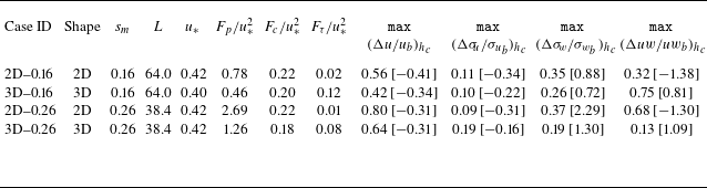


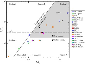


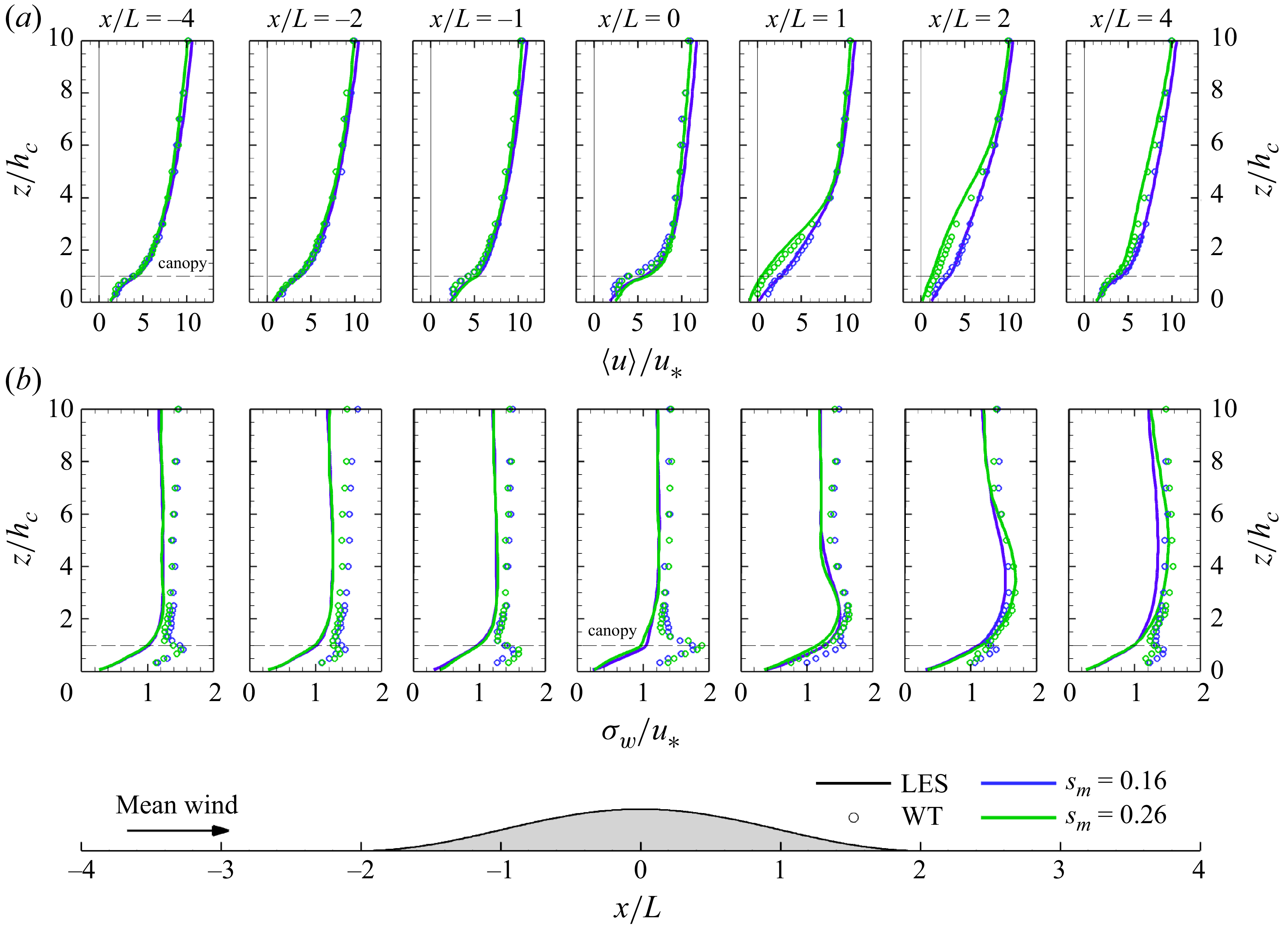


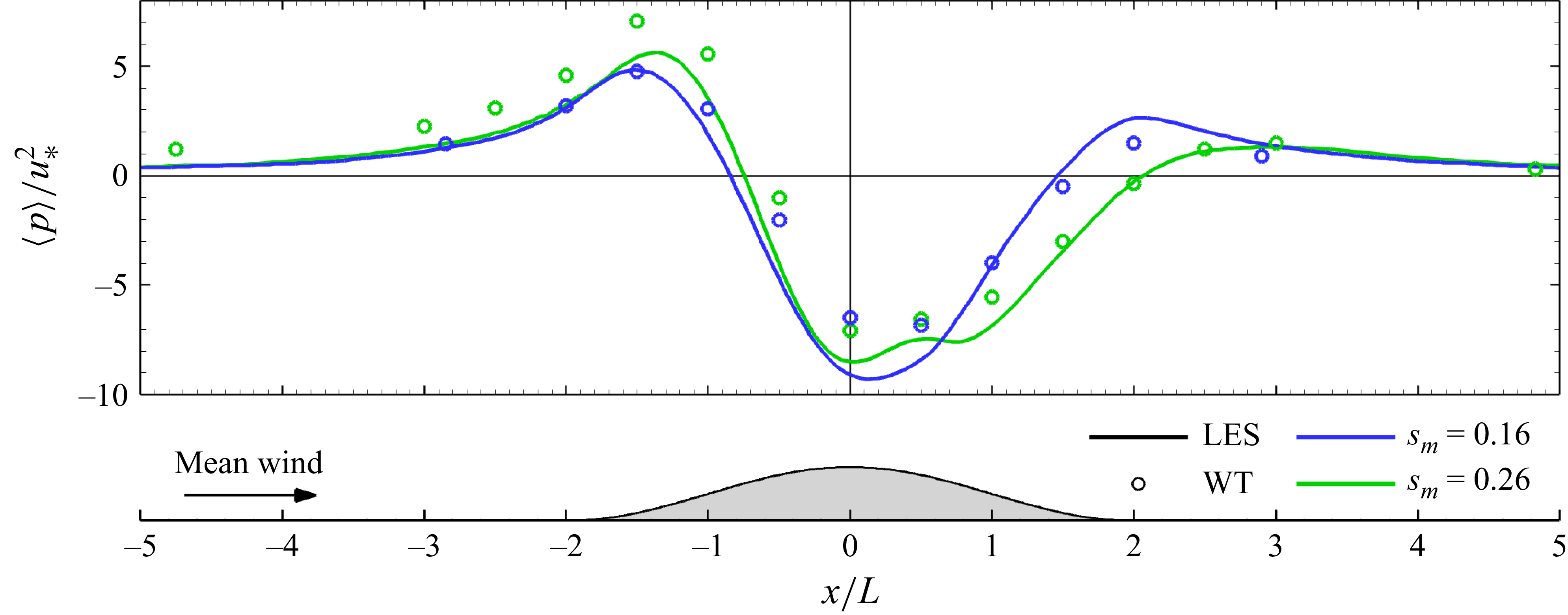


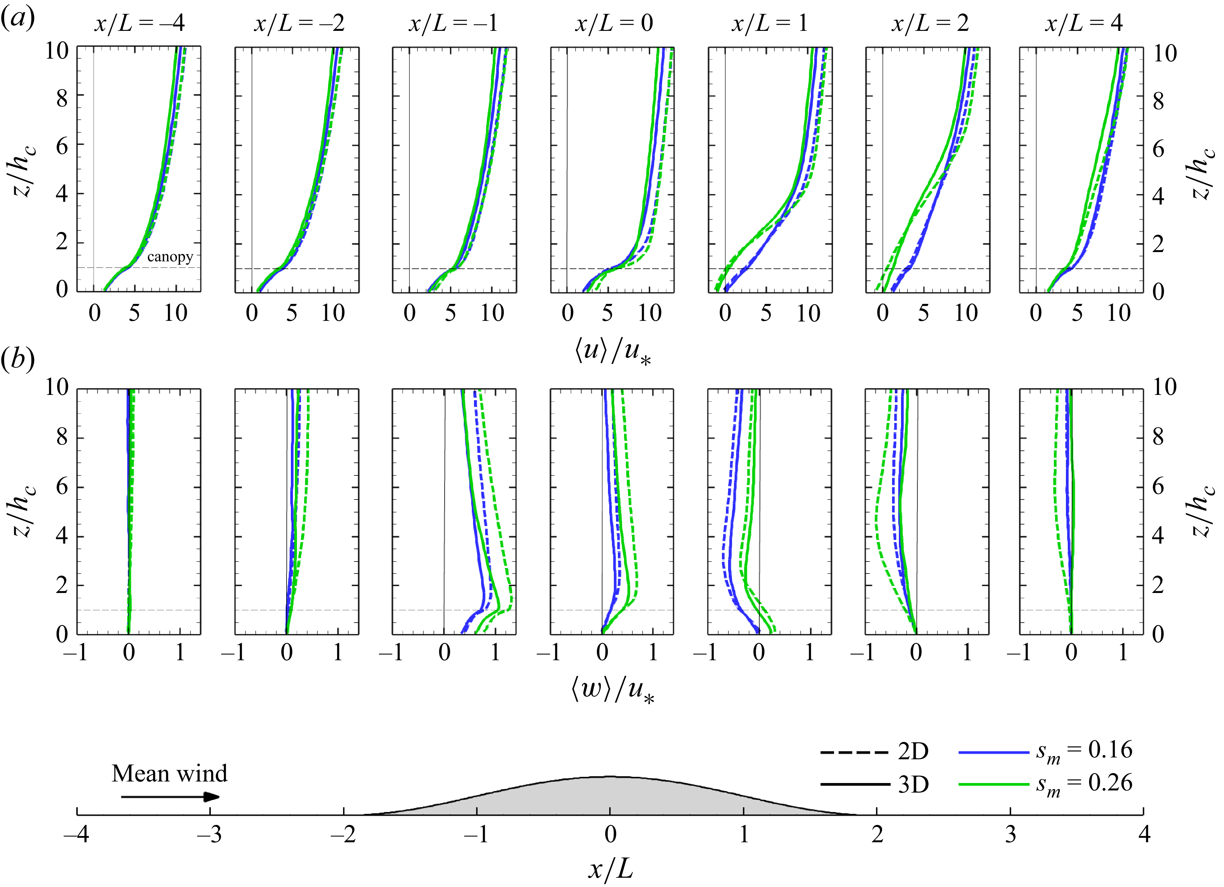


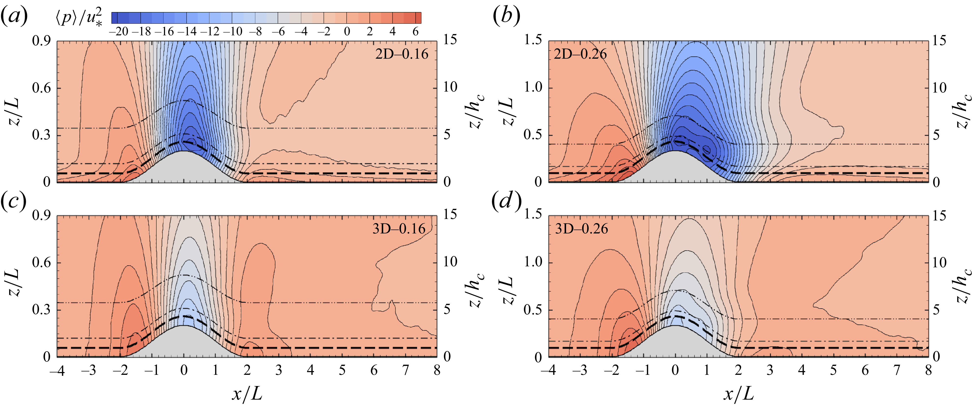


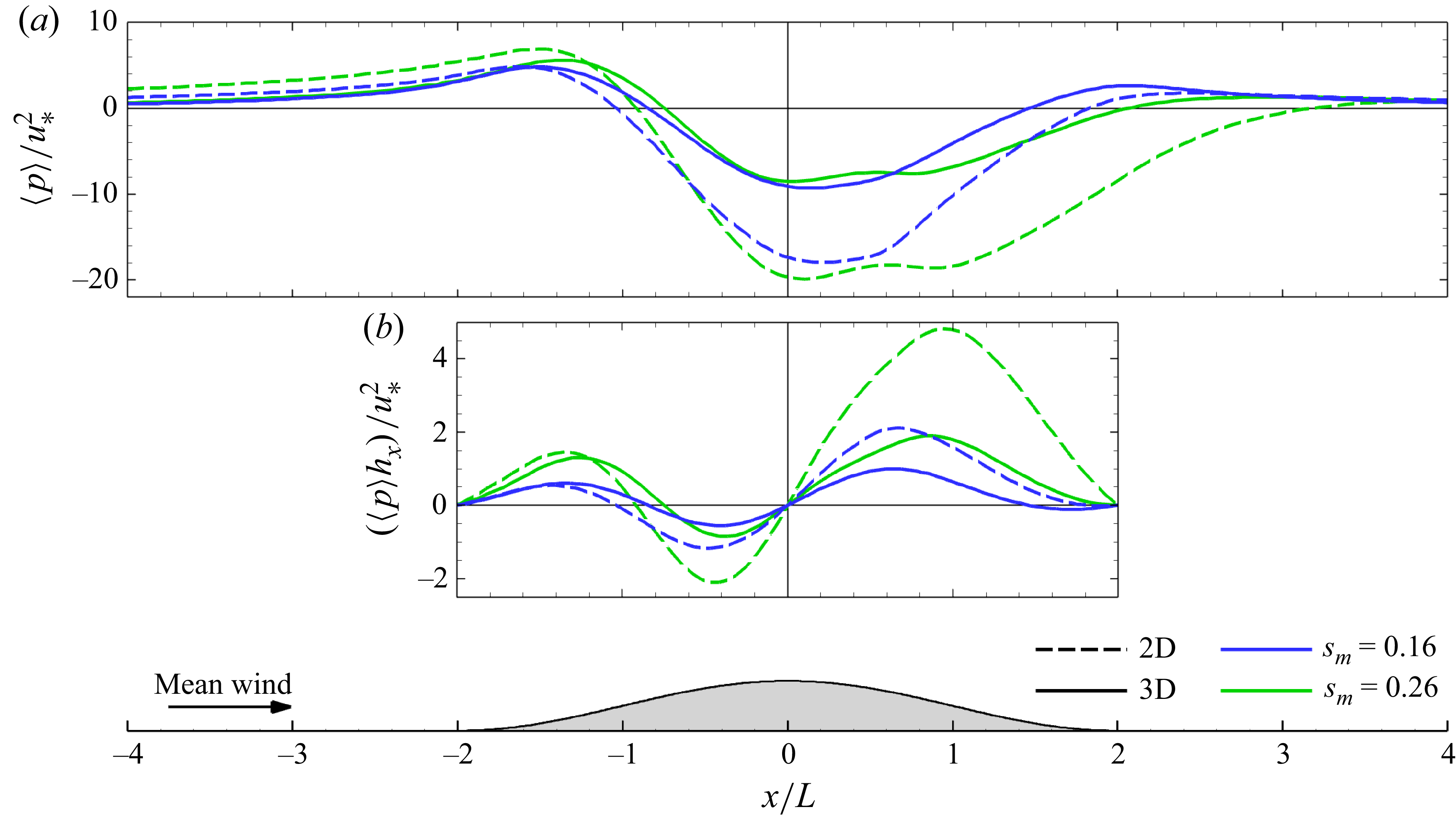


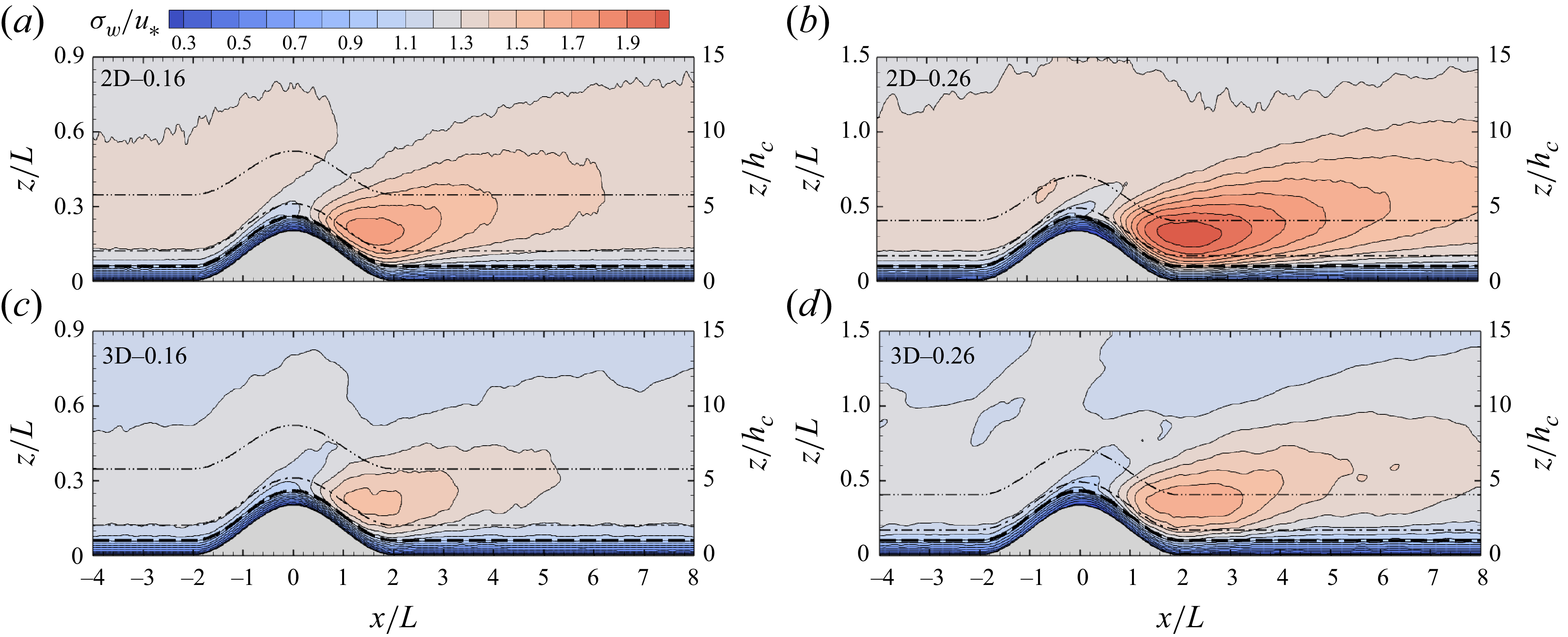


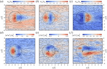


 Open access