





1. Introduction
Axisymmetric flows arise in a variety of applications, including flows through annuli and pipes as well as round jets, and their stability has long been of considerable interest. In most practical situations, the Reynolds number is high, so viscous effects may be neglected. The inviscid approximation greatly simplifies the stability equations and often leads to fruitful mathematical results. An important contribution to the inviscid stability of axisymmetric base flows was made by Batchelor & Gill (Reference Batchelor and Gill1962), who derived a convenient sufficient condition for stability. This result can be viewed as an extension of the well-known Rayleigh–Fjortoft stability condition for parallel flows (Rayleigh Reference Rayleigh1880; Fjørtoft Reference Fjørtoft1950). Although significant progress has since been made in the inviscid stability analysis of parallel base flows, somewhat surprisingly, applications to axisymmetric base flows remain scarce.
Arnol’d (Reference Arnol’d1966) showed that two distinct sufficient conditions for stability exist through a pseudoenergy-based analysis, which is now known as Arnol’d’s method (see Shepherd Reference Shepherd1993 also). Earlier, Lord Kelvin had also suggested the presence of two such conditions (Thomson Reference Thomson1880). Owing to this historical development, those stability conditions are called the Kelvin–Arnol’d first and second shear-stability theorems (KA-I and KA-II). The Rayleigh–Fjørtoft condition corresponds to KA-I, as does the result of Batchelor & Gill (Reference Batchelor and Gill1962). For parallel flows, the KA-II conditions have also been well studied, particularly in the context of instabilities in planetary atmospheres (see Stamp & Dowling Reference Stamp and Dowling1993; Dowling Reference Dowling2020; Read & Dowling Reference Read and Dowling2026, for example). Therefore, one might expect that the KA-II condition could also be applied to axisymmetric base flows to yield useful stability criteria; however, no such results have been explicitly derived in the literature.
Except for a few special cases, the KA stability conditions generally fail to sharply detect points of neutral stability, as first demonstrated in the pioneering work of Tollmien (Reference Tollmien1935). This limitation has motivated efforts to identify classes of base flows that admit sharp stability criteria and to simplify those criteria as much as possible. For example, Rosenbluth & Simon (Reference Rosenbluth and Simon1964) and Balmforth & Morrison (Reference Balmforth and Morrison1999) employed the Nyquist method, whereas Barston (Reference Barston1991) and Hirota, Morrison & Hattori (Reference Hirota, Morrison and Hattori2014) drew inspiration from the properties of certain quadratic forms. Despite being more numerically tractable than the full eigenvalue problem, these approaches still rely on the solution to a Fredholm integral equation or similarly complex criteria.
Recently, Deguchi, Hirota & Dowling (Reference Deguchi, Hirota and Dowling2024) derived a simple sufficient condition for instability. The condition essentially depends on whether the reciprocal Rossby–Mach number, derived from the base flow, surpasses a threshold called the hurdle. Since this can be conveniently assessed using a simple graphical procedure, the result is referred to as the hurdle theorem. Although this condition does not sharply determine the neutral point, plotting the regions in parameter space where the hurdle theorem and the KA criteria hold allows one to roughly estimate the location of neutral points. In practice, this helps restrict the parameter range that needs to be explored in the eigenvalue problem.
The proof by Deguchi et al. (Reference Deguchi, Hirota and Dowling2024) follows the two-step approach that became popular after the seminal work of Howard (Reference Howard1964): (i) first, demonstrate the existence of a neutral solution, and (ii) then show that an unstable mode emerges when this neutral state is perturbed. The essence of this approach can already be found in Tollmien (Reference Tollmien1935). A mathematically rigorous proof of step (ii) was later provided by Lin (Reference Lin2003), and more recently simplified by Kumar & Ożański (Reference Kumar and Ożański2025). In step (i), the neutral solution is constructed through minimisation of the Rayleigh quotient. The central idea of Deguchi et al. (Reference Deguchi, Hirota and Dowling2024) is to analytically derive a simple condition ensuring the existence of a neutral solution by estimating the minimum value with a suitable trial function.
In this paper, we extend the sufficient stability condition of Batchelor & Gill (Reference Batchelor and Gill1962) and derive a simple sufficient condition for instability for axisymmetric base flows. The former is obtained following the aforementioned KA-II framework, while the latter is derived by generalising the hurdle theorem. For annular flows, the analysis proceeds in much the same way as for parallel flows, although the azimuthal wavenumber of the perturbations must be treated carefully. Pipe flows, however, require additional consideration, and the conditions must be modified from those for the annular case to obtain satisfactory results.
The proposed stability conditions are applied to representative model flows to assess their practical usefulness. More specifically, we consider cases where shear flow and thermal convection coexist. Parallel shear flows, whether driven by a pressure gradient or by moving boundaries, tend to be inviscidly stable, as exemplified by plane Couette flow or plane Poiseuille flow. The first model flow we consider is sliding Couette flow (an annular version of Couette flow, see Gittler Reference Gittler1993; Deguchi & Nagata Reference Deguchi and Nagata2011), coupled with thermal convection due to the temperature difference between the walls. The flow is designed so that, in the absence of the wall sliding effect, the system reduces to natural convection in a vertical annulus, a configuration frequently studied in the natural convection literature (Choi & Korpela Reference Choi and Korpela1980; Yao & Rogers Reference Yao and Rogers1989; Kang, Yang & Mutabazi Reference Kang, Yang and Mutabazi2015; Wang & Chen Reference Wang and Chen2022). The second model is a vertically oriented Hagen–Poiseuille flow with homogeneous internal heating. This model can be regarded as the pipe analogue of the channel model flow used to test the hurdle theorem in Deguchi et al. (Reference Deguchi, Hirota and Dowling2024), and it was also investigated by Senoo, Deguchi & Nagata (Reference Senoo, Deguchi and Nagata2012) and Marensi, He & Willis (Reference Marensi, He and Willis2021). The performance of the stability conditions will be assessed by comparing their predictions with the numerically obtained neutral points. Those inviscid stability results are further compared with linearised Navier–Stokes computations.
The structure of the paper is as follows. In the next section, we formulate the stability problem for axisymmetric base flows. Numerical methods for both inviscid and viscous stability problems are also introduced. Section 3 summarises the sufficient conditions for stability and instability derived in this paper. These conditions are applied to model flows in annuli and pipes in § 4, with their derivation presented in § 5. Finally, § 6 presents the conclusions. In the same section, we also discuss the implications of the present results for round jets, which originally motivated the work of Batchelor & Gill (Reference Batchelor and Gill1962).
2. Formulation of the problem
2.1. Inviscid stability problem for axisymmetric base flows
Let $\boldsymbol{u}=u_r\boldsymbol{e}_r+u_{\varphi }\boldsymbol{e}_{\varphi }+u_z\boldsymbol{e}_z$
and
$\boldsymbol{u}=u_r\boldsymbol{e}_r+u_{\varphi }\boldsymbol{e}_{\varphi }+u_z\boldsymbol{e}_z$
and $p$
denote the velocity and pressure of an incompressible fluid in cylindrical coordinates
$p$
denote the velocity and pressure of an incompressible fluid in cylindrical coordinates $(r,\varphi ,z)$
, with
$(r,\varphi ,z)$
, with $\boldsymbol{e}_r$
,
$\boldsymbol{e}_r$
, $\boldsymbol{e}_{\varphi }$
and
$\boldsymbol{e}_{\varphi }$
and $\boldsymbol{e}_z$
the associated unit vectors. Periodicity of
$\boldsymbol{e}_z$
the associated unit vectors. Periodicity of $2\pi /k$
is imposed in the
$2\pi /k$
is imposed in the $z$
direction, with
$z$
direction, with $k$
denoting the axial wavenumber. We assume a steady axisymmetric base flow
$k$
denoting the axial wavenumber. We assume a steady axisymmetric base flow $\boldsymbol{u}=U(r)\boldsymbol{e}_z$
directed along the axial direction, and assess its stability by examining the evolution of infinitesimal perturbations
$\boldsymbol{u}=U(r)\boldsymbol{e}_z$
directed along the axial direction, and assess its stability by examining the evolution of infinitesimal perturbations $\tilde {\boldsymbol{u}}=\tilde {u}_r\boldsymbol{e}_r+\tilde {u}_{\varphi }\boldsymbol{e}_{\varphi }+\tilde {u}_z\boldsymbol{e}_z$
superposed on it. The azimuthal wavenumber of the perturbation is denoted by
$\tilde {\boldsymbol{u}}=\tilde {u}_r\boldsymbol{e}_r+\tilde {u}_{\varphi }\boldsymbol{e}_{\varphi }+\tilde {u}_z\boldsymbol{e}_z$
superposed on it. The azimuthal wavenumber of the perturbation is denoted by $n$
. The physical requirement of
$n$
. The physical requirement of $2\pi$
periodicity in the
$2\pi$
periodicity in the $\varphi$
direction implies that
$\varphi$
direction implies that $n$
must be an integer.
$n$
must be an integer.
The stability of the flow can be analysed by solving the linearised Navier–Stokes equations; if viscosity is neglected, the analysis can begin with the linearised Euler equations. Batchelor & Gill (Reference Batchelor and Gill1962) showed that the latter inviscid stability problem boils down to solving the differential equation
 \begin{align} \left\{\frac {r}{N^2+r^2}(rG)^{\prime} \right \}^{\prime}-k^2G+\frac {Q^{\prime}}{U-c}rG=0,\qquad Q=\frac {-rU^{\prime}}{N^2+ r^2}, \end{align}
with suitable boundary conditions. Here, a prime denotes ordinary differentiation with respect to radius, $r$
. For a fixed wavenumber ratio
$r$
. For a fixed wavenumber ratio $N = n/k$
, (2.1) together with suitable boundary conditions constitutes an eigenvalue problem, with the complex phase speed
$N = n/k$
, (2.1) together with suitable boundary conditions constitutes an eigenvalue problem, with the complex phase speed $c=c_r+ic_i$
as the eigenvalue. By symmetry, it suffices to consider
$c=c_r+ic_i$
as the eigenvalue. By symmetry, it suffices to consider $k \gt 0$
and
$k \gt 0$
and $n \geqslant 0$
. From the eigenfunction
$n \geqslant 0$
. From the eigenfunction $G(r)$
, the perturbation field can be reconstructed as
$G(r)$
, the perturbation field can be reconstructed as
 \begin{align} \,[\tilde {u}_r,\tilde {u}_{\varphi },\tilde {u}_{z},\tilde {p}]=[iG(r),H(r),F(r),P(r)]e^{in\varphi +ik(z-ct)}+\text{c.c.}, \end{align}
where
 \begin{align} \left [ \begin{array}{c} F\\ H \end{array} \right ] &= \frac {1}{k(N^2+r^2)} \left [ \begin{array}{cc} -N & -r\\ r & -N \end{array} \right ] \left [ \begin{array}{c} NU^{\prime}G/(U-c)\\ rG^{\prime}+G \end{array} \right ], \end{align}
 \begin{align} P &=-(U-c)F-k^{-1}U^{\prime}G, \end{align}
and c.c. denotes the complex conjugate. The existence of an eigenvalue with $c_i \gt 0$
indicates the presence of disturbances that grow exponentially with time
$c_i \gt 0$
indicates the presence of disturbances that grow exponentially with time $t$
, and hence the flow is unstable. The flow is said to be stable when no such unstable mode exists (the mode with
$t$
, and hence the flow is unstable. The flow is said to be stable when no such unstable mode exists (the mode with $c_i=0$
is neutrally stable).
$c_i=0$
is neutrally stable).
The general properties of the inviscid stability problem (2.1) are the main focus of this paper. For concreteness, however, we examine the stability conditions for specific base flows. The model base flows to be introduced in § 4 can be described using the Navier–Stokes equations together with the Boussinesq approximation. We specifically consider the case of an infinitesimally small Prandtl number, for which the stability problem reduces to the linearised Navier–Stokes equations. Note that, since the Prandtl number is the ratio of viscous to thermal diffusion, a small value implies that the diffusion term dominates advection in the temperature equation. Consequently, temperature perturbations decay and the buoyancy term is removed from the momentum equations for perturbations (see Lignières Reference Lignières1999 for example).
Section 4.1 examines a flow between coaxial cylinders, while § 4.2 studies a pipe flow. For the annular geometry, we set the inner and outer cylinder walls at $r=r_i$
and
$r=r_i$
and $r=r_o$
. The radius ratio
$r=r_o$
. The radius ratio $\eta =r_i/r_o \leqslant 1$
is the only parameter needed to specify the geometry. Under the non-dimensionalisation in which the gap is set to 2
$\eta =r_i/r_o \leqslant 1$
is the only parameter needed to specify the geometry. Under the non-dimensionalisation in which the gap is set to 2
 \begin{align} r_i=2\eta /(1-\eta ), \qquad r_o=2/(1-\eta ). \end{align}
The no-penetration boundary condition then requires that $G$
vanishes at the walls.
$G$
vanishes at the walls.
For the pipe flow problem, physical quantities are required to be regular at the centreline. If we assume that the perturbation velocity field is Taylor expandable about the pipe axis in Cartesian coordinates, then $G$
has the following expansion (see Eisen, Heinrichs & Witsch Reference Eisen, Heinrichs and Witsch1991):
$G$
has the following expansion (see Eisen, Heinrichs & Witsch Reference Eisen, Heinrichs and Witsch1991):
 \begin{align} G=\mathcal{G}_1r+\mathcal{G}_3r^3+\ldots , \,\,\,\,&\text{if}\,\,\,\, n= 0, \end{align}
 \begin{align} G=\mathcal{G}_{n-1}r^{n-1}+\mathcal{G}_{n+1}r^{n+1}+\ldots \,\,\,\,&\text{if}\,\,\,\, n\neq 0. \end{align}
Therefore, the eigenfunction for the pipe problem is expected to satisfy
 \begin{align} G^{\prime}=0, \,\,\,\,\text{if}\,\,\,\, n= 1, \end{align}
 \begin{align} G=0 \,\,\,\,\text{if}\,\,\,\, n\neq 1, \end{align}
at $r=0$
. Note that (2.7) is not a boundary condition of (2.1). This conclusion follows from the standard singularity theory of ordinary differential equations. As commented in Lessen & Singh (Reference Lessen and Singh1973), the method of Frobenius expansion yields that one of the linearly independent solutions is singular, while the other, non-singular solution satisfies (2.7).
$r=0$
. Note that (2.7) is not a boundary condition of (2.1). This conclusion follows from the standard singularity theory of ordinary differential equations. As commented in Lessen & Singh (Reference Lessen and Singh1973), the method of Frobenius expansion yields that one of the linearly independent solutions is singular, while the other, non-singular solution satisfies (2.7).
2.2. Numerical method
The eigenvalue problem (2.1) can be solved using the Chebyshev-collocation method, in which $G(r)$
is expanded by the basis functions
$G(r)$
is expanded by the basis functions $\varPsi _l(r)$
 \begin{align} G(r)=\sum _{l=0}^L \hat {G}_l \varPsi _l(r). \end{align}
The annular case is straightforward. We use the basis $\varPsi _l(r)=(1-y^2)T_l(y)$
, where
$\varPsi _l(r)=(1-y^2)T_l(y)$
, where $T_l(y)$
are the Chebyshev polynomials in the shifted variable
$T_l(y)$
are the Chebyshev polynomials in the shifted variable $y=r-r_m$
. To map
$y=r-r_m$
. To map $y$
into the interval
$y$
into the interval $(-1,1)$
, we set
$(-1,1)$
, we set $r_m=(r_o+r_i)/2$
, the mid-gap. Collocation points are chosen as
$r_m=(r_o+r_i)/2$
, the mid-gap. Collocation points are chosen as $r_j=r_m+\cos (({j+1})/({L+2})\pi )$
,
$r_j=r_m+\cos (({j+1})/({L+2})\pi )$
, $j=0,1,\ldots ,L$
.
$j=0,1,\ldots ,L$
.
For the pipe case, we checked the consistency of the numerical codes using the following two methods:
-
(i) Expand $G$
in modified Chebyshev polynomials (see Deguchi & Walton Reference Deguchi and Walton2013)(2.9)The governing equation is then evaluated at the collocation points
\begin{align} \varPsi _l(r)= \left \{ \begin{array}{c} (1-r^2)T_{2l+1}(r),\qquad \text{if $n$ is even},\qquad \\ (1-r^2)T_{2l}(r),\qquad \,\,\, \text{if $n$ is odd}. \end{array} \right . \end{align}
$r_j=\cos ((j+1)\pi /(2L+4)), j=0,1,\ldots ,L$
.
$G$
in modified Chebyshev polynomials (see Deguchi & Walton Reference Deguchi and Walton2013)(2.9)The governing equation is then evaluated at the collocation points
\begin{align} \varPsi _l(r)= \left \{ \begin{array}{c} (1-r^2)T_{2l+1}(r),\qquad \text{if $n$ is even},\qquad \\ (1-r^2)T_{2l}(r),\qquad \,\,\, \text{if $n$ is odd}. \end{array} \right . \end{align}
$r_j=\cos ((j+1)\pi /(2L+4)), j=0,1,\ldots ,L$
.
-
(ii) Treat the domain as an annulus with a virtual inner cylinder of small radius
$\epsilon \gt 0$
, and impose condition (2.7) there. The code developed in Song & Dong (Reference Song and Dong2023) is used, which employs the fourth-order compact finite-difference scheme (see Malik Reference Malik1990). We choose
$\epsilon =0.001$
.


The results of the inviscid analysis are compared with the calculations of the following linearised Navier–Stokes equations
 \begin{align} k(U-c)G &=P^{\prime}-\frac {i}{Re} \left(G^{\prime \prime}+\frac {G^{\prime}}{r}- \left(k^2+\frac {n^2+1}{r^2}\right)G-\frac {2n}{r^2}H \right), \end{align}
 \begin{align} k(U-c)H &=-\frac {n}{r}P-\frac {i}{Re}\left(H^{\prime \prime}+\frac {H^{\prime}}{r}-\left(k^2+\frac {n^2+1}{r^2}\right)H-\frac {2n}{r^2}G\right), \end{align}
 \begin{align} k(U-c)F+U^{\prime}G &=-kP-\frac {i}{Re}\left(F^{\prime \prime}+\frac {F^{\prime}}{r}-\left(k^2+\frac {n^2}{r^2}\right)F\right), \end{align}
 \begin{align} G^{\prime}+\frac {G}{r} &+\frac {n}{r}H+kF =0, \end{align}
where $Re$
is the Reynolds number. To solve the above eigenvalue problem, we employed a numerical code using the Chebyshev-collocation method originally developed by Deguchi & Nagata (Reference Deguchi and Nagata2011) for the annular domain. For the pipe flow problem, the basis functions are replaced with those of Deguchi & Walton (Reference Deguchi and Walton2013). The codes have been thoroughly tested and validated against results from other research groups (see, e.g. Deguchi Reference Deguchi2017; He et al. Reference He, Deguchi, Song and Blackburn2025).
$Re$
is the Reynolds number. To solve the above eigenvalue problem, we employed a numerical code using the Chebyshev-collocation method originally developed by Deguchi & Nagata (Reference Deguchi and Nagata2011) for the annular domain. For the pipe flow problem, the basis functions are replaced with those of Deguchi & Walton (Reference Deguchi and Walton2013). The codes have been thoroughly tested and validated against results from other research groups (see, e.g. Deguchi Reference Deguchi2017; He et al. Reference He, Deguchi, Song and Blackburn2025).
3. Stability conditions
Throughout the paper, we assume that $U(r)$
possesses
$U(r)$
possesses $C^1$
smoothness in
$C^1$
smoothness in $\varOmega$
(i.e. the first derivative is continuous in the domain). Here, for the annular case,
$\varOmega$
(i.e. the first derivative is continuous in the domain). Here, for the annular case, $\varOmega =(r_i,r_o)$
, and for the pipe case,
$\varOmega =(r_i,r_o)$
, and for the pipe case, $\varOmega =(0,1)$
. For the pipe problem, we further assume that the even extension of
$\varOmega =(0,1)$
. For the pipe problem, we further assume that the even extension of $U(r)$
is
$U(r)$
is $C^1$
in
$C^1$
in $(-1,1)$
.
$(-1,1)$
.
To state the main result of this paper, it is convenient to define
 \begin{align} W_{\alpha ,N}(r)=\frac {rQ^{\prime}}{U-\alpha }. \end{align}
Batchelor & Gill (Reference Batchelor and Gill1962) also used a similar quantity in their analysis; however, note that our $Q$
is defined differently from theirs. The right-hand side of (3.1) depends on a constant
$Q$
is defined differently from theirs. The right-hand side of (3.1) depends on a constant $\alpha$
and the wavenumber ratio
$\alpha$
and the wavenumber ratio $N$
via
$N$
via $Q$
, hence the subscripts.
$Q$
, hence the subscripts.
The main results of this paper are presented in the following theorems, which provide convenient criteria for assessing the inviscid stability problem (2.1).
Theorem 1.
The base flow is stable if the KA-I and/or KA-II conditions are satisfied for all $N$
.
$N$
.
-
(i) KA-I: There exists
$\alpha \in \mathbb{R}$
such that
$W_{\alpha ,N}\leqslant 0$
for all
$r \in \varOmega$
. -
(ii) KA-II: There exists
$\beta \in \mathbb{R}$
such that
$W_{\beta ,N}=({rQ^{\prime}}/({U-\beta }))\in [0,H(r)]$
for all
$r \in \varOmega$
. Here,
(3.2)for the annular case,
\begin{align} H=\left \{ \begin{array}{c} \left(\frac {\pi }{\ln \eta }\right)^2 \frac {1}{N^2+r_o^2}+\frac {1}{N^2}\qquad \text{if} \qquad N\geqslant 1,\\ \left(\frac {\pi }{\ln \eta }\right)^2 \frac {1}{r_o^2} \qquad \quad \qquad \text{if} \qquad N= 0 ,\end{array} \right . \end{align}
(3.3)for the pipe case (
\begin{align} H=\left \{ \begin{array}{c} (j_{1,1}^2r^2+N^{-2})/(N^2+1)\qquad \text{if} \qquad N\geqslant 1,\\ j_{1,1}^2 \qquad \text{if} \qquad N= 0 ,\end{array} \right. \end{align}
$j_{1,1}\approx 3.8317$
is the first positive zero of the Bessel function of the first kind of order one).


Theorem 2.
The base flow is unstable if the following conditions are satisfied for some $N$
:
$N$
:
-
(i)
$Q^{\prime}(r)$
has only one zero at
$r=r_c$
and it is isolated. -
(ii)
$Q^{\prime \prime}(r_c)\neq 0$
. -
(iii)
$U^{\prime}(r_c)\neq 0$
. -
(iv)
$W_{\alpha ,N}\gt h(r)$
with
$\alpha =U(r_c)$
for all
$r\in \varOmega$
. Here,(3.4)for the annular case,
\begin{align} h=\frac {(\pi /\ln \eta )^2}{N^2+ r_i^2}+\frac {1}{N^2} , \end{align}
(3.5)for the pipe case.
\begin{align} h=Cr^p, \qquad p\geqslant 2, \qquad C=\frac {1}{\rho _p}\left(\rho _N+\frac {1}{6N^2}\right)\!,\nonumber \\ \rho _N=\frac {(3N^2+1)^2}{2}\ln \left(\frac {N^2+1}{N^2}\right)-\frac {3(6N^2+1)}{4},\nonumber \\ \rho _p=\frac {8}{(p+2)(p+4)(p+6)}, \end{align}


Theorem 1 corresponds to KA-I and KA-II for axisymmetric base flows, and guarantees regions in parameter space where the base flow is stable. KA-I is due to Batchelor & Gill (Reference Batchelor and Gill1962), whereas KA-II is a new result. Note that when $Q^{\prime}$
has no zeros for any
$Q^{\prime}$
has no zeros for any $N$
, the base flow is stable, since in this case one can choose
$N$
, the base flow is stable, since in this case one can choose $|\alpha |$
sufficiently large to fulfil the KA-I condition. This is an extension of Rayleigh’s inflection point theorem.
$|\alpha |$
sufficiently large to fulfil the KA-I condition. This is an extension of Rayleigh’s inflection point theorem.
Theorem 2 serves as a handy means of demonstrating the existence of instability in the parameter space. It extends the hurdle theorem by Deguchi et al. (Reference Deguchi, Hirota and Dowling2024); instability emerges when $W_{\alpha ,N}$
surpasses the hurdle
$W_{\alpha ,N}$
surpasses the hurdle $h$
. Deguchi et al. (Reference Deguchi, Hirota and Dowling2024) defined the ‘reciprocal Rossby–Mach number’ so that the hurdle height equals unity, inspired by studies of Jupiter’s jets. An analogous quantity can be defined by multiplying
$h$
. Deguchi et al. (Reference Deguchi, Hirota and Dowling2024) defined the ‘reciprocal Rossby–Mach number’ so that the hurdle height equals unity, inspired by studies of Jupiter’s jets. An analogous quantity can be defined by multiplying $W_{\alpha ,N}$
by a constant factor. Readers interested in the interpretation of our stability conditions using that number are referred to Appendix A.4.
$W_{\alpha ,N}$
by a constant factor. Readers interested in the interpretation of our stability conditions using that number are referred to Appendix A.4.
The proofs of above theorems are given in § 5.
4. Analysis of model profiles
4.1. Flow through an annulus
Consider the flow of a fluid between co-axial cylinders whose common axis is aligned with gravity (see figure 1 a). The fluid motion is driven by two effects: the differential axial movement of the cylinders and buoyancy resulting from an imposed temperature difference between the cylinders.
The annular model flow used in § 4.1. (a) Schematic of the model flow in the dimensional cylindrical coordinates $(r_*,\varphi ,z_*)$
. Here, the radii
$(r_*,\varphi ,z_*)$
. Here, the radii $r_{i*}$
and
$r_{i*}$
and $r_{o*}$
satisfy
$r_{o*}$
satisfy $r_{o*}-r_{i*}=2d_*$
,
$r_{o*}-r_{i*}=2d_*$
, $r_{i*}/r_{o*}=\eta$
. (b) The base flow
$r_{i*}/r_{o*}=\eta$
. (b) The base flow $U(r)$
given in (4.5) for
$U(r)$
given in (4.5) for $\chi =-7,-1,1,7$
.
$\chi =-7,-1,1,7$
.

We take half of the cylinder gap $d_*$
, half of the differential speed
$d_*$
, half of the differential speed $u_*$
and half of the imposed temperature difference
$u_*$
and half of the imposed temperature difference $\Delta \theta _*$
as the characteristic length, velocity and temperature scales, respectively. The non-dimensional Navier–Stokes equations under the Boussinesq approximation yield the governing equations for the axial base velocity
$\Delta \theta _*$
as the characteristic length, velocity and temperature scales, respectively. The non-dimensional Navier–Stokes equations under the Boussinesq approximation yield the governing equations for the axial base velocity $U(r)$
and the base temperature
$U(r)$
and the base temperature $\varTheta (r)$
 \begin{align} \varTheta^{\prime \prime}+r^{-1}\varTheta^{\prime} &=0, \end{align}
 \begin{align} U^{\prime \prime}+r^{-1}U^{\prime} &=\chi \varTheta . \end{align}
The left-hand sides represent diffusivity, while the term proportional to $\chi$
corresponds to buoyancy. The ratio of the Grashof number
$\chi$
corresponds to buoyancy. The ratio of the Grashof number $Gr$
to the Reynolds number
$Gr$
to the Reynolds number $Re$
defines the parameter
$Re$
defines the parameter $\chi$
as follows:
$\chi$
as follows:
 \begin{align} \chi =\frac {Gr}{Re},\qquad Gr=\frac {\gamma _*g_* d_*^3 \Delta \theta _*}{\nu _*^2},\qquad Re=\frac {u_*h_*}{\nu _*}. \end{align}
Here, $g_*$
denotes the gravitational acceleration,
$g_*$
denotes the gravitational acceleration, $\gamma _*$
the thermal expansion coefficient and
$\gamma _*$
the thermal expansion coefficient and $\nu _*$
the kinematic viscosity of the fluid. The boundary conditions are
$\nu _*$
the kinematic viscosity of the fluid. The boundary conditions are
 \begin{align} U=1, \,\,\varTheta =-1\qquad \text{at}\qquad r=r_i, \end{align}
 \begin{align} U=-1, \,\,\varTheta =1\qquad \text{at}\qquad r=r_o. \end{align}
The limit $\chi \rightarrow 0$
corresponds to sliding Couette flow (Gittler Reference Gittler1993; Deguchi & Nagata Reference Deguchi and Nagata2011), while for large
$\chi \rightarrow 0$
corresponds to sliding Couette flow (Gittler Reference Gittler1993; Deguchi & Nagata Reference Deguchi and Nagata2011), while for large $|\chi |$
, the system approaches natural convection in a vertical annulus (Choi & Korpela Reference Choi and Korpela1980; Yao & Rogers Reference Yao and Rogers1989; Kang et al. Reference Kang, Yang and Mutabazi2015; Wang & Chen Reference Wang and Chen2022).
$|\chi |$
, the system approaches natural convection in a vertical annulus (Choi & Korpela Reference Choi and Korpela1980; Yao & Rogers Reference Yao and Rogers1989; Kang et al. Reference Kang, Yang and Mutabazi2015; Wang & Chen Reference Wang and Chen2022).
The solution of (4.1) with the boundary conditions (4.3) is given by
 \begin{align} \varTheta &= C_1 \ln r+C_2, \end{align}
 \begin{align} U &= C_3\ln r+C_4 +\frac {\chi }{4} r^2(C_1-C_2- C_1 \ln r ), \end{align}
where
 \begin{align} C_1=-\frac {2}{\ln \eta }, \quad C_2=-1- C_1\ln r_i, \quad C_3=\frac {C_5-C_6}{\ln \eta }, \quad C_4=C_5-C_3\ln r_i,\nonumber \\ C_5=1+ \chi \frac {r_i^2}{4}\{ C_1\ln r_i-C_1+C_2 \},\qquad C_6=-1+\chi \frac {r_o^2}{4}\{ C_1 \ln r_o-C_1+C_2 \}. \end{align}
The base flow depends on $\eta$
and
$\eta$
and $\chi$
. Figure 1(b) shows the profiles at
$\chi$
. Figure 1(b) shows the profiles at $\eta =0.7$
for various values of
$\eta =0.7$
for various values of $\chi$
.
$\chi$
.
The function $Q$
defined in (2.1) is readily found. Its derivative, required for computation of
$Q$
defined in (2.1) is readily found. Its derivative, required for computation of $W_{\alpha ,N}$
in (3.1), is given by
$W_{\alpha ,N}$
in (3.1), is given by
 \begin{align} Q^{\prime}=r\frac {N^2\chi (C_2+C_1\ln r)+2C_3+\chi r^2 \frac {C_1}{2}}{(N^2+r^2)^2}. \end{align}
If $N$
is sufficiently large,
$N$
is sufficiently large, $Q^{\prime}$
varies monotonically and therefore has at most one zero. This is convenient for applying Theorem 2.
$Q^{\prime}$
varies monotonically and therefore has at most one zero. This is convenient for applying Theorem 2.
Figure 2 summarises the inviscid stability in the $\eta$
–
$\eta$
– $\chi$
parameter plane. The blue region indicates stability guaranteed by Theorem 1, while the red region indicates instability guaranteed by Theorem 2. As expected, the neutral curve obtained by numerically solving the differential equation (the solid black line) lies between the two regions.
$\chi$
parameter plane. The blue region indicates stability guaranteed by Theorem 1, while the red region indicates instability guaranteed by Theorem 2. As expected, the neutral curve obtained by numerically solving the differential equation (the solid black line) lies between the two regions.
Stability diagram of the annular model flow (figure 1
a) in the $\chi$
–
$\chi$
– $\eta$
plane. All physically possible wavenumbers are covered. The black solid line represents the neutral curve of the inviscid problem (2.1). Stability is guaranteed by Theorem 1 in the blue region, while unstable modes are found by Theorem 2 in the red region.
$\eta$
plane. All physically possible wavenumbers are covered. The black solid line represents the neutral curve of the inviscid problem (2.1). Stability is guaranteed by Theorem 1 in the blue region, while unstable modes are found by Theorem 2 in the red region.

In the limit $\eta \rightarrow 1$
, the analysis becomes particularly simple, so we begin our discussion from this case. This limit, referred to as the narrow-gap limit, corresponds to
$\eta \rightarrow 1$
, the analysis becomes particularly simple, so we begin our discussion from this case. This limit, referred to as the narrow-gap limit, corresponds to $r_i,r_o\rightarrow \infty$
in our non-dimensionalisation where the gap width is set to 2. We introduce the new variable
$r_i,r_o\rightarrow \infty$
in our non-dimensionalisation where the gap width is set to 2. We introduce the new variable $y=r-r_m \in (-1,1)$
, where
$y=r-r_m \in (-1,1)$
, where $r_m=(r_o+r_i)/2$
is the mid-gap. Taking the limit
$r_m=(r_o+r_i)/2$
is the mid-gap. Taking the limit $N\rightarrow \infty$
and
$N\rightarrow \infty$
and $\eta \rightarrow 1$
while keeping
$\eta \rightarrow 1$
while keeping $N\ll r_m$
, we obtain
$N\ll r_m$
, we obtain
 \begin{align} W_{\alpha ,N}=-\frac {1}{U-\alpha }\frac {d^2U}{{\textrm{d}}y^2},\qquad H=h=\left(\frac {\pi }{2}\right)^2, \end{align}
from (3.1), (3.2) and (3.4). Theorem 2 reduces to the hurdle theorem for parallel flows derived in Deguchi et al. (Reference Deguchi, Hirota and Dowling2024). The limiting form of the base flow is
 \begin{align} U=\frac {\chi }{6}y(y^2-1)-y. \end{align}
The numerator of $W_{\alpha ,N}$
, i.e.
$W_{\alpha ,N}$
, i.e. $ {d^2U}/{{\textrm{d}}y^2}$
, vanishes only at
$ {d^2U}/{{\textrm{d}}y^2}$
, vanishes only at $y=y_c=0$
. Setting
$y=y_c=0$
. Setting $\alpha =U(y_c)=0$
, we have
$\alpha =U(y_c)=0$
, we have
 \begin{align} W_{\alpha ,N}=\frac {6\chi }{6+\chi (1-y^2)}. \end{align}
The results of applying Theorems 1 and 2 for the narrow-gap limit case, shown in figure 3, can be understood as follows. When $\chi \gt 0$
, the maximum of
$\chi \gt 0$
, the maximum of $W_{\alpha ,N}$
is
$W_{\alpha ,N}$
is $\chi$
and the minimum is
$\chi$
and the minimum is $6\chi /(6+\chi )$
. Therefore, for
$6\chi /(6+\chi )$
. Therefore, for $\chi \in (0,( {\pi }/{2})^2)$
, where
$\chi \in (0,( {\pi }/{2})^2)$
, where $( {\pi }/{2})^2\approx 2.47$
, the KA-II condition of Theorem 1 is satisfied. Moreover, when
$( {\pi }/{2})^2\approx 2.47$
, the KA-II condition of Theorem 1 is satisfied. Moreover, when $6\chi /(6+\chi )\gt ({\pi }/{2})^2$
, that is, for
$6\chi /(6+\chi )\gt ({\pi }/{2})^2$
, that is, for $\chi \gt {6\pi ^2}/{24-\pi ^2}\approx 4.19$
, Theorem 2 guarantees the existence of an instability. When
$\chi \gt {6\pi ^2}/{24-\pi ^2}\approx 4.19$
, Theorem 2 guarantees the existence of an instability. When $\chi \in (-6,0)$
, the KA-I condition in Theorem 1 is satisfied. For
$\chi \in (-6,0)$
, the KA-I condition in Theorem 1 is satisfied. For $\chi \leqslant -6$
, neither theorem can be applied, since the numerator of (4.10) vanishes at
$\chi \leqslant -6$
, neither theorem can be applied, since the numerator of (4.10) vanishes at $y=\pm \sqrt {1+6/\chi }$
and
$y=\pm \sqrt {1+6/\chi }$
and $W_{\alpha ,N}$
is not continuous. By numerically solving the Rayleigh equation,
$W_{\alpha ,N}$
is not continuous. By numerically solving the Rayleigh equation,
 \begin{align} \frac {d^2G}{{\textrm{d}}y^2}-k^2G-\frac {\frac {d^2U}{{\textrm{d}}y^2}}{U-c} G=0, \qquad G(-1)=G(1)=0, \end{align}
we find that the true neutral point occurs at $\chi \approx 3.810$
. Note that in the narrow-gap limit, Squire’s theorem implies that the stability is independent of the wavenumber ratio. Hence, there is no need to consider
$\chi \approx 3.810$
. Note that in the narrow-gap limit, Squire’s theorem implies that the stability is independent of the wavenumber ratio. Hence, there is no need to consider $N$
at all.
$N$
at all.
Stability diagram of the annular model flow at the narrow-gap limit $\eta \rightarrow 1$
. The eigenvalue problem (4.11) indicates the presence of unstable modes for
$\eta \rightarrow 1$
. The eigenvalue problem (4.11) indicates the presence of unstable modes for $\chi \lt -6$
and
$\chi \lt -6$
and $\chi \gt 3.81$
. The grey line shows that the profile of
$\chi \gt 3.81$
. The grey line shows that the profile of $W_{\alpha ,N}$
, given in (4.10), becomes singular when
$W_{\alpha ,N}$
, given in (4.10), becomes singular when $\chi \leqslant -6$
.
$\chi \leqslant -6$
.

Even for $\eta \lt 1$
, the behaviour of
$\eta \lt 1$
, the behaviour of $W_{\alpha ,N}$
remains qualitatively similar to the narrow-gap case, as illustrated in figure 4 for
$W_{\alpha ,N}$
remains qualitatively similar to the narrow-gap case, as illustrated in figure 4 for $\eta =0.7$
. However, the results now depend on
$\eta =0.7$
. However, the results now depend on $N$
, since Squire’s theorem no longer applies. In the figure, we choose
$N$
, since Squire’s theorem no longer applies. In the figure, we choose $N=10$
. Panel (a) illustrates the case
$N=10$
. Panel (a) illustrates the case $\chi =7$
, where
$\chi =7$
, where $W_{\alpha ,N}$
surpasses the hurdle
$W_{\alpha ,N}$
surpasses the hurdle $h$
(defined in (3.4) and shown by the red line). The location
$h$
(defined in (3.4) and shown by the red line). The location $r=r_c$
indicates where
$r=r_c$
indicates where $Q^{\prime}$
in (4.7) vanishes. When
$Q^{\prime}$
in (4.7) vanishes. When $\chi$
is reduced to 1, as shown in panel (b), the KA-II condition of Theorem 1 is satisfied; the blue line in the figure indicates
$\chi$
is reduced to 1, as shown in panel (b), the KA-II condition of Theorem 1 is satisfied; the blue line in the figure indicates $H$
in (3.2). Panel (c) is the case where
$H$
in (3.2). Panel (c) is the case where $\chi =-1$
, for which
$\chi =-1$
, for which $W_{\alpha ,N}$
is everywhere negative, and hence the flow is stable for
$W_{\alpha ,N}$
is everywhere negative, and hence the flow is stable for $N=10$
perturbations by KA-I (i.e. the result by Batchelor & Gill Reference Batchelor and Gill1962). Panel (d) corresponds to
$N=10$
perturbations by KA-I (i.e. the result by Batchelor & Gill Reference Batchelor and Gill1962). Panel (d) corresponds to $\chi =-7$
, which lies below the lower boundary of the stable region (blue) shown in figure 2. In this case,
$\chi =-7$
, which lies below the lower boundary of the stable region (blue) shown in figure 2. In this case, $W_{\alpha ,N}$
cannot be made continuous for any choice of
$W_{\alpha ,N}$
cannot be made continuous for any choice of $\alpha$
, and neither Theorem 1 nor Theorem 2 can be used to determine stability.
$\alpha$
, and neither Theorem 1 nor Theorem 2 can be used to determine stability.
Profiles of $W_{\alpha ,N}$
with
$W_{\alpha ,N}$
with $N=10$
for the annular model flow at
$N=10$
for the annular model flow at $\eta =0.7$
. The constant
$\eta =0.7$
. The constant $\alpha$
is set equal to
$\alpha$
is set equal to $U(r_c)$
. Panels show (a)
$U(r_c)$
. Panels show (a) $\chi =7$
; (b)
$\chi =7$
; (b) $\chi =1$
; (c)
$\chi =1$
; (c) $\chi =-1$
; (d)
$\chi =-1$
; (d) $\chi =-7$
. In panel (a), the red line shows
$\chi =-7$
. In panel (a), the red line shows $h$
from (3.4). In panel (b), the blue line shows
$h$
from (3.4). In panel (b), the blue line shows $H$
defined in (3.2).
$H$
defined in (3.2).

Figure 4 shows only the case for $N=10$
, but physically, perturbations with all values of
$N=10$
, but physically, perturbations with all values of $N$
can occur. Therefore, to use Theorem 1 to establish stability, it is not sufficient to examine only a handful of
$N$
can occur. Therefore, to use Theorem 1 to establish stability, it is not sufficient to examine only a handful of $N$
values. In figure 2, we verified the reliability of the blue stable region using a wide range of
$N$
values. In figure 2, we verified the reliability of the blue stable region using a wide range of $N$
values. Note that the limit
$N$
values. Note that the limit $N\rightarrow \infty$
is straightforward to analyse. This means that for sufficiently large
$N\rightarrow \infty$
is straightforward to analyse. This means that for sufficiently large $N$
, asymptotic behaviour emerges, so in practice it is sufficient to examine the conditions of the theorem up to moderately large
$N$
, asymptotic behaviour emerges, so in practice it is sufficient to examine the conditions of the theorem up to moderately large $N$
. Likewise, at each point in the parameter plane, the value of
$N$
. Likewise, at each point in the parameter plane, the value of $N$
is optimised to maximise the red unstable region. However, fixing
$N$
is optimised to maximise the red unstable region. However, fixing $N=10$
yields almost the same outcome as that in figure 2. This suggests that identifying the unstable region using Theorem 2 is easier than finding the stable region using Theorem 1.
$N=10$
yields almost the same outcome as that in figure 2. This suggests that identifying the unstable region using Theorem 2 is easier than finding the stable region using Theorem 1.
The neutral curve in figure 2 is also obtained by optimising over the wavenumbers $k$
and
$k$
and $n$
: above the black line an unstable mode is found for some
$n$
: above the black line an unstable mode is found for some $(k,n)$
, while below it no unstable mode exists for any choice of
$(k,n)$
, while below it no unstable mode exists for any choice of $(k,n)$
.
$(k,n)$
.
Figure 5 shows $c_i$
obtained from numerical computations of (2.1) for
$c_i$
obtained from numerical computations of (2.1) for $\eta =0.7$
and
$\eta =0.7$
and $\chi =7$
. Panel (a) is computed with
$\chi =7$
. Panel (a) is computed with $N=10$
; hence at
$N=10$
; hence at $k=0.1$
, the mode with
$k=0.1$
, the mode with $n=Nk=1$
exhibits instability, as expected by Theorem 2. The neutral solution at
$n=Nk=1$
exhibits instability, as expected by Theorem 2. The neutral solution at $k=0.502$
is non-physical because
$k=0.502$
is non-physical because $n=5.02$
is not an integer. Physically admissible neutral solutions can be obtained by reducing
$n=5.02$
is not an integer. Physically admissible neutral solutions can be obtained by reducing $N$
. For example, choosing
$N$
. For example, choosing $N=1/0.9475$
yields a neutral point at
$N=1/0.9475$
yields a neutral point at $k=k_0=0.9475$
, i.e.
$k=k_0=0.9475$
, i.e. $n=1$
. Panel (b) shows the corresponding eigenfunction. This function is free of singularities due to the regularity of
$n=1$
. Panel (b) shows the corresponding eigenfunction. This function is free of singularities due to the regularity of $W_{\alpha ,N}$
. The red dashed line in panel (a) shows an analytic linear approximation of how
$W_{\alpha ,N}$
. The red dashed line in panel (a) shows an analytic linear approximation of how $c_i$
behaves near the neutral point. As will be shown in § 5.2 (see (5.23)), we can derive the identity
$c_i$
behaves near the neutral point. As will be shown in § 5.2 (see (5.23)), we can derive the identity
 \begin{align} \left . \frac {{\textrm{d}}c_i}{{\textrm{d}}k}\right |_{k=k_0} =-\frac {2k_0K_i}{K_r^2+K_i^2}\int _{\varOmega }rG_0^2{\textrm{d}}r, \end{align}
where
 \begin{align} K_r=\lim _{\epsilon \rightarrow 0}\left\{\int _{r_i}^{r_c-\epsilon }\frac {r^2Q^{\prime}G_0^2}{(U-\alpha )^2}{\textrm{d}}r+\int ^{r_o}_{r_c+\epsilon }\frac {r^2Q^{\prime}G_0^2}{(U-\alpha )^2}{\textrm{d}}r\right\}, \quad K_i=\pi \left . \left (\frac {rW_{\alpha ,N}G_0^2}{|U^{\prime}|} \right ) \right |_{r=r_c} \end{align}
can be found using the neutral wavenumber $k_0$
, the regular neutral eigenfunction
$k_0$
, the regular neutral eigenfunction $G_0$
and
$G_0$
and $\alpha =U(r_c)$
. The right-hand side of (4.12) is evaluated as
$\alpha =U(r_c)$
. The right-hand side of (4.12) is evaluated as $-0.886$
, which gives the slope of the red dashed line. As similar results hold for
$-0.886$
, which gives the slope of the red dashed line. As similar results hold for $N\approx 1/0.9475$
, one can conclude that a slight increase of
$N\approx 1/0.9475$
, one can conclude that a slight increase of $N$
from its neutral value necessarily results in the emergence of an unstable mode with
$N$
from its neutral value necessarily results in the emergence of an unstable mode with $n=1$
. The observation here highlights the strategy to be used in § 5.2 for proving Theorem 2.
$n=1$
. The observation here highlights the strategy to be used in § 5.2 for proving Theorem 2.
Inviscid stability result for the annular model flow at $(\eta ,\chi )=(0.7,7)$
. (a) Imaginary part of the phase speed
$(\eta ,\chi )=(0.7,7)$
. (a) Imaginary part of the phase speed $c_i$
for
$c_i$
for $N=10$
. The neutral point is at
$N=10$
. The neutral point is at $k=k_0=0.502$
. The dashed red line indicates the result using (4.12). (b) Eigenfunction of the neutral mode found at
$k=k_0=0.502$
. The dashed red line indicates the result using (4.12). (b) Eigenfunction of the neutral mode found at $N=1/k$
,
$N=1/k$
, $k=0.9475$
(i.e.
$k=0.9475$
(i.e. $n=1$
).
$n=1$
).

Along the neutral curve in figure 2, the eigenfunction is regular. However, when $W_{\alpha ,N}$
is singular (as in figure 4
d), neutral solutions with singularities at the critical levels (i.e. locations where
$W_{\alpha ,N}$
is singular (as in figure 4
d), neutral solutions with singularities at the critical levels (i.e. locations where $U=c$
) may arise. In the parameter plane shown in figure 2, such singular modes indeed occur when
$U=c$
) may arise. In the parameter plane shown in figure 2, such singular modes indeed occur when $\chi$
lies slightly below the lower boundary of the stable region. A detailed check in the narrow-gap limit confirmed that the neutral point lies very close to
$\chi$
lies slightly below the lower boundary of the stable region. A detailed check in the narrow-gap limit confirmed that the neutral point lies very close to $\chi =-6$
(see figure 3). The computation was performed using 30 000 grid points in order to capture the nearly singular eigenfunctions with small
$\chi =-6$
(see figure 3). The computation was performed using 30 000 grid points in order to capture the nearly singular eigenfunctions with small $c_i$
. Likewise, the blue lower stability boundary in figure 2 may lie very close to the neutral curve, but we do not go into further detail. Note that such nearly singular unstable modes cannot be captured by Theorem 2 and are therefore outside the scope of the present study.
$c_i$
. Likewise, the blue lower stability boundary in figure 2 may lie very close to the neutral curve, but we do not go into further detail. Note that such nearly singular unstable modes cannot be captured by Theorem 2 and are therefore outside the scope of the present study.
Figure 6 confirms the above inviscid stability results through computations of the linearised Navier–Stokes equation, (2.10). The dashed line indicates the neutral curve obtained by optimising over wavenumbers $k$
,
$k$
, $n$
. The most unstable mode is always
$n$
. The most unstable mode is always $n=1$
, which asymptotes to the inviscid result
$n=1$
, which asymptotes to the inviscid result $\chi =3.86$
as
$\chi =3.86$
as $Re$
increases. The stability for
$Re$
increases. The stability for $Re\gt 10^4$
is relatively well captured by Theorems 1 and 2.
$Re\gt 10^4$
is relatively well captured by Theorems 1 and 2.
Comparison between the viscous and inviscid stability analyses for the annular model flow at $\eta =0.7$
. The dashed line represents the neutral curve obtained from the viscous stability problem (2.10), covering all physically possible wavenumbers. The blue, black and red vertical lines correspond to the inviscid stability results shown in figure 2.
$\eta =0.7$
. The dashed line represents the neutral curve obtained from the viscous stability problem (2.10), covering all physically possible wavenumbers. The blue, black and red vertical lines correspond to the inviscid stability results shown in figure 2.

4.2. Flow through a pipe
In this section, we consider vertically oriented Hagen–Poiseuille flow with homogeneous internal heating (figure 7
a, see Senoo et al. Reference Senoo, Deguchi and Nagata2012; Marensi et al. Reference Marensi, He and Willis2021 also). We choose the pipe radius $d_*$
as the length scale, and the centreline velocity of the laminar Hagen–Poiseuille flow
$d_*$
as the length scale, and the centreline velocity of the laminar Hagen–Poiseuille flow $u_*$
as the velocity scale. For the temperature scale, we use the difference
$u_*$
as the velocity scale. For the temperature scale, we use the difference $\Delta \theta _*$
between the base temperature at the centreline,
$\Delta \theta _*$
between the base temperature at the centreline, $\theta _{0*}+\Delta \theta _*$
, and that at the wall,
$\theta _{0*}+\Delta \theta _*$
, and that at the wall, $\theta _{0*}$
. The velocity and temperature scales are related to the dimensional axial pressure gradient
$\theta _{0*}$
. The velocity and temperature scales are related to the dimensional axial pressure gradient $\Delta p_*/L_*$
and the dimensional internal heat source
$\Delta p_*/L_*$
and the dimensional internal heat source $q_*$
as follows:
$q_*$
as follows:
 \begin{align} u_*=\frac {d_*^2}{4\mu _*}\frac {\Delta p_*}{L_*},\qquad \theta _*=\frac {d_*^2q_*}{4\kappa _*}. \end{align}
Here, $\mu _*$
is the dynamic viscosity and
$\mu _*$
is the dynamic viscosity and $\kappa _*$
is the thermal diffusivity of the fluid.
$\kappa _*$
is the thermal diffusivity of the fluid.


From the Boussinesq-approximated Navier–Stokes equations, the equations for the axial base velocity $U(r)$
and the base temperature
$U(r)$
and the base temperature $\varTheta (r)$
are obtained as
$\varTheta (r)$
are obtained as
 \begin{align} \varTheta^{\prime \prime}+r^{-1}\varTheta^{\prime} &=-4, \end{align}
 \begin{align} U^{\prime \prime}+r^{-1}U^{\prime} &=\chi \varTheta -4. \end{align}
The solutions of the above equations, satisfying the boundary conditions
 \begin{align} U=0, \,\,\varTheta =0\qquad \text{at}\qquad r=1, \end{align}
and the centreline regularity, are
 \begin{align} \varTheta &=(1-r^2), \end{align}
 \begin{align} U &=(1-r^2)-\frac {\chi }{16}(1-r^2)(3-r^2). \end{align}
The base flow profiles for selected values of $\chi$
are shown in figure 7(b). An inflection point appears when
$\chi$
are shown in figure 7(b). An inflection point appears when $\chi$
is in a certain range, and by analogy with Rayleigh’s theorem, Senoo et al. (Reference Senoo, Deguchi and Nagata2012) speculated that this could be a possible cause of instability. However, the mathematics of inviscid instability is not that simple.
$\chi$
is in a certain range, and by analogy with Rayleigh’s theorem, Senoo et al. (Reference Senoo, Deguchi and Nagata2012) speculated that this could be a possible cause of instability. However, the mathematics of inviscid instability is not that simple.
Substituting the base flow $U$
into the definition of
$U$
into the definition of $Q$
(see (2.1)) and differentiating, we obtain
$Q$
(see (2.1)) and differentiating, we obtain
 \begin{align} Q^{\prime}=r\frac {N^2(4-\chi (1-r^2))+\frac {\chi }{2}r^4}{(N^2+r^2)^2}. \end{align}
It is easy to see that $Q^{\prime}$
vanishes at
$Q^{\prime}$
vanishes at $r=r_c$
, where
$r=r_c$
, where
 \begin{align} r_c=N\sqrt {\sqrt {1+\frac {2}{N^2}\big(1-\frac {4}{\chi }\big)}-1 }. \end{align}
Clearly, the axisymmetric mode is stable, since for $N=0$
, the function
$N=0$
, the function $Q^{\prime}$
does not change sign in the domain (the KA-I condition is satisfied, see the remark in § 3). Even for non-axisymmetric modes, the parameter range
$Q^{\prime}$
does not change sign in the domain (the KA-I condition is satisfied, see the remark in § 3). Even for non-axisymmetric modes, the parameter range $\chi \in (0,4)$
remains stable, as no real
$\chi \in (0,4)$
remains stable, as no real $r_c$
exists. Determining inviscid stability for other values of
$r_c$
exists. Determining inviscid stability for other values of $\chi$
is not trivial, but by applying Theorems 1 and 2, we can find the results shown in figure 8.
$\chi$
is not trivial, but by applying Theorems 1 and 2, we can find the results shown in figure 8.


When $\chi$
is negative, either KA-I or KA-II holds. Figure 9(a) shows the profile of
$\chi$
is negative, either KA-I or KA-II holds. Figure 9(a) shows the profile of $W_{\alpha ,N}$
for
$W_{\alpha ,N}$
for $\chi =-10$
and
$\chi =-10$
and $N=1$
. This is an example in which the KA-II condition defined in (3.3) is satisfied;
$N=1$
. This is an example in which the KA-II condition defined in (3.3) is satisfied; $W_{\alpha ,N}$
is positive everywhere and lies below
$W_{\alpha ,N}$
is positive everywhere and lies below $H$
indicated by the blue line.
$H$
indicated by the blue line.


For $\chi \in [5.72,7.42]$
, there exist
$\chi \in [5.72,7.42]$
, there exist $N\gt 0$
and
$N\gt 0$
and $p\geqslant 2$
such that
$p\geqslant 2$
such that $W_{\alpha ,N}$
exceeds the hurdle (3.5). Figure 9(c) shows the profile of
$W_{\alpha ,N}$
exceeds the hurdle (3.5). Figure 9(c) shows the profile of $W_{\alpha ,N}$
for
$W_{\alpha ,N}$
for $\chi =7$
and
$\chi =7$
and $N=1$
. In this figure, the hurdle for
$N=1$
. In this figure, the hurdle for $p=2$
is indicated by the red line. Thus, by Theorem 2, the flow is unstable. Note that a horizontal hurdle, as used in the annular case, does not work well for the pipe flow since near
$p=2$
is indicated by the red line. Thus, by Theorem 2, the flow is unstable. Note that a horizontal hurdle, as used in the annular case, does not work well for the pipe flow since near $r=0$
,
$r=0$
, $W_{\alpha ,N}$
behaves like
$W_{\alpha ,N}$
behaves like $r^2$
. Figure 10(a) shows the eigenvalue analysis of (2.1) for
$r^2$
. Figure 10(a) shows the eigenvalue analysis of (2.1) for $\chi =7$
and
$\chi =7$
and $N=1$
. This calculation uses method (ii) of § 2.2, with the condition
$N=1$
. This calculation uses method (ii) of § 2.2, with the condition $G^{\prime}(\epsilon )=0$
. At
$G^{\prime}(\epsilon )=0$
. At $k=1$
, we indeed have an unstable mode with
$k=1$
, we indeed have an unstable mode with $n=1$
.
$n=1$
.
Inviscid stability result for the pipe model flow at $\chi =7$
. (a) Imaginary part of the phase speed
$\chi =7$
. (a) Imaginary part of the phase speed $c_i$
for
$c_i$
for $N=1$
. The neutral point is at
$N=1$
. The neutral point is at $k=k_0=1.159$
. The dashed red line indicates the result using (4.12). (b) Eigenfunction of the neutral mode found at
$k=k_0=1.159$
. The dashed red line indicates the result using (4.12). (b) Eigenfunction of the neutral mode found at $N=1/k$
,
$N=1/k$
, $k=1.46$
(i.e.
$k=1.46$
(i.e. $n=1$
).
$n=1$
).

The red dashed line in figure 10(a) corresponds to results similar to those seen in figure 5(a). The slope $-0.0549$
is obtained by the neutral mode using (4.12). By decreasing the value of
$-0.0549$
is obtained by the neutral mode using (4.12). By decreasing the value of $N$
from 1 to
$N$
from 1 to $1/k$
with
$1/k$
with $k=1.46$
, a neutral mode with
$k=1.46$
, a neutral mode with $n=1$
is obtained. This neutral mode is regular as shown in figure 10(b). We confirmed that the methods (i) and (ii) introduced in § 2.2 produce eigenfunctions that are graphically indistinguishable.
$n=1$
is obtained. This neutral mode is regular as shown in figure 10(b). We confirmed that the methods (i) and (ii) introduced in § 2.2 produce eigenfunctions that are graphically indistinguishable.
By computing neutral points using (2.1) for all physically admissible wavenumbers, it is found that a neutral point occurs at $\chi =7.86$
(see figure 8). This value is reasonably close to the unstable region predicted by Theorem 2. The eigenvalue problem (2.1) does not produce unstable modes for
$\chi =7.86$
(see figure 8). This value is reasonably close to the unstable region predicted by Theorem 2. The eigenvalue problem (2.1) does not produce unstable modes for $\chi \gt 7.86$
. This stabilisation can be detected by KA-II when
$\chi \gt 7.86$
. This stabilisation can be detected by KA-II when $\chi \gt 13.18$
. For example, figure 9(d) shows the case
$\chi \gt 13.18$
. For example, figure 9(d) shows the case $\chi =14$
,
$\chi =14$
, $N=1$
, where
$N=1$
, where $W_{\alpha ,N}$
lies below the blue line
$W_{\alpha ,N}$
lies below the blue line $H$
determined by (3.3).
$H$
determined by (3.3).
Another neutral point is expected to exist between the blue stability region and the red instability region in figure 8. The computations of (2.1) indicates that instability sets in when $\chi$
slightly exceeds 4, implying that the stability boundary
$\chi$
slightly exceeds 4, implying that the stability boundary $\chi =4$
by Theorem 1 sharply predicts the neutral point. The eigenfunction corresponding to this neutral point is singular. Hence, it makes sense that the boundary of the unstable region by Theorem 2 is not sharp. Careful observation of
$\chi =4$
by Theorem 1 sharply predicts the neutral point. The eigenfunction corresponding to this neutral point is singular. Hence, it makes sense that the boundary of the unstable region by Theorem 2 is not sharp. Careful observation of $W_{\alpha ,N}$
shows that it becomes singular for some
$W_{\alpha ,N}$
shows that it becomes singular for some $N$
when
$N$
when $\chi \in [4,6]$
. An example of such a singular case is shown in figure 9(b), obtained for
$\chi \in [4,6]$
. An example of such a singular case is shown in figure 9(b), obtained for $\chi =5$
and
$\chi =5$
and $N=1$
.
$N=1$
.
Figure 11 verifies the above inviscid results using viscous computations. The dashed line represents the envelope of the neutral curves obtained from the linearised Navier–Stokes equations (2.10) over a range of wavenumbers. This curve is determined by the $n=1$
mode and asymptotes to the inviscid neutral points at
$n=1$
mode and asymptotes to the inviscid neutral points at $\chi =4$
and
$\chi =4$
and $7.86$
for large Reynolds numbers. Recall that for
$7.86$
for large Reynolds numbers. Recall that for $\chi \in [4,6]$
, instability may arise from the singular neutral mode, whereas for
$\chi \in [4,6]$
, instability may arise from the singular neutral mode, whereas for $\chi \in [5.72,7.42]$
, Theorem 2 guarantees the existence of regular neutral modes. The neutral curve found by the viscous analysis features two humps, representing two unstable modes, which correspond to a singular mode and a regular mode in the inviscid analysis.
$\chi \in [5.72,7.42]$
, Theorem 2 guarantees the existence of regular neutral modes. The neutral curve found by the viscous analysis features two humps, representing two unstable modes, which correspond to a singular mode and a regular mode in the inviscid analysis.

5. Mathematical proofs
Here, we prove Theorems 1 and 2 stated in § 3. For definiteness, we introduce the function space $H_0^1$
, following the standard notation in functional analysis. For
$H_0^1$
, following the standard notation in functional analysis. For $f \in H_0^1$
, both
$f \in H_0^1$
, both $\int _{\varOmega } (f^{\prime})^2 r,{\textrm{d}}r$
and
$\int _{\varOmega } (f^{\prime})^2 r,{\textrm{d}}r$
and $\int _{\varOmega } f^2 r,{\textrm{d}}r$
are finite, and the boundary conditions are satisfied. Specifically, in the annular case,
$\int _{\varOmega } f^2 r,{\textrm{d}}r$
are finite, and the boundary conditions are satisfied. Specifically, in the annular case, $f(r_i)=f(r_o)=0$
, while in the pipe case,
$f(r_i)=f(r_o)=0$
, while in the pipe case, $f(1)=0$
. Recall that the pipe solution also satisfy the centreline regularity condition (2.6). If
$f(1)=0$
. Recall that the pipe solution also satisfy the centreline regularity condition (2.6). If $G$
satisfies (2.1) in the classical sense, then
$G$
satisfies (2.1) in the classical sense, then $G \in H_0^1$
.
$G \in H_0^1$
.
5.1. Proof of Theorem 1
Following Batchelor & Gill (Reference Batchelor and Gill1962), we multiply (2.1) by the complex conjugate of $rG$
and integrate over the entire domain
$rG$
and integrate over the entire domain $\varOmega$
. The real and imaginary parts of the integral are obtained as
$\varOmega$
. The real and imaginary parts of the integral are obtained as
 \begin{align} \int _{\varOmega } \left\{\frac {r}{N^2+ r^2}|(rG)^{\prime}|^2 +\frac {k^2}{r}|rG|^2-\frac {Q^{\prime}(U-c_r)}{|U-c|^2}|rG|^2 \right\}{\textrm{d}}r & =0, \end{align}
 \begin{align} c_i\int _{\varOmega } \frac {Q^{\prime}}{|U-c|^2}|rG|^2{\textrm{d}}r &=0, \end{align}
respectively. The boundary terms arising from integration by parts vanish in all cases we consider.
Now, we assume $c_i\neq 0$
and show that the KA-I assumption leads to a contradiction. This can be found in the same manner as Fjortoft’s analysis for parallel flows. By taking a suitable linear combination of the two integrals (5.1) and (5.2), we obtain
$c_i\neq 0$
and show that the KA-I assumption leads to a contradiction. This can be found in the same manner as Fjortoft’s analysis for parallel flows. By taking a suitable linear combination of the two integrals (5.1) and (5.2), we obtain
 \begin{align} \int _{\varOmega } \left\{\frac {r}{N^2+r^2}|(rG)^{\prime}|^2 +\frac {k^2}{r}|rG|^2-W_{\alpha ,N}\frac {(U-\alpha )^2}{|U-c|^2}\frac {|rG|^2}{r} \right\}{\textrm{d}}r=0, \end{align}
where $\alpha \in \mathbb{R}$
is arbitrary. If
$\alpha \in \mathbb{R}$
is arbitrary. If $W_{\alpha ,N}=rQ^{\prime}/(U-\alpha )\leqslant 0$
for all
$W_{\alpha ,N}=rQ^{\prime}/(U-\alpha )\leqslant 0$
for all $r \in \varOmega$
, the above integral cannot be satisfied for non-trivial
$r \in \varOmega$
, the above integral cannot be satisfied for non-trivial $G$
. The analysis here is identical to that in Batchelor & Gill (Reference Batchelor and Gill1962) but included for completeness.
$G$
. The analysis here is identical to that in Batchelor & Gill (Reference Batchelor and Gill1962) but included for completeness.
KA-II stability is usually derived by defining a Hamiltonian. However, in our case, an equivalent condition can be obtained in a more straightforward manner. We first set $\alpha =2c_r-\beta$
to rewrite (5.3) in the form
$\alpha =2c_r-\beta$
to rewrite (5.3) in the form
 \begin{align} \int _{\varOmega } \left\{\frac {r}{N^2+ r^2}|(rG)^{\prime}|^2 +\frac {k^2}{r}|rG|^2-W_{\beta ,N}Z\frac {|rG|^2}{r} \right\}{\textrm{d}}r=0, \end{align}
where $Z= ({(U-c_r)^2-(c_r-\beta )^2})/({(U-c_r)^2+c_i^2})\lt 1$
. The choice of
$Z= ({(U-c_r)^2-(c_r-\beta )^2})/({(U-c_r)^2+c_i^2})\lt 1$
. The choice of $\beta \in \mathbb{R}$
is arbitrary; by assumption, it can be adjusted so that
$\beta \in \mathbb{R}$
is arbitrary; by assumption, it can be adjusted so that $W_{\beta ,N}\in [0,H(r))$
for
$W_{\beta ,N}\in [0,H(r))$
for $r\in \varOmega$
. From this point onward, the analysis must be treated separately for annular and pipe flows.
$r\in \varOmega$
. From this point onward, the analysis must be treated separately for annular and pipe flows.
For the annular problem, there is a positive constant $\kappa _N^2$
depending on
$\kappa _N^2$
depending on $N$
such that
$N$
such that
 \begin{align} \int _{r_i}^{r_o} \frac {r}{N^2+ r^2}|(rf)^{\prime}|^2 {\textrm{d}}r\geqslant \kappa _N^2 \int _{r_i}^{r_o} r^{-1}|rf|^2{\textrm{d}}r, \end{align}
for all $f(r) \in H_0^1$
; this is a generalisation of Poincaré’s inequality. Using the non-negativity of
$f(r) \in H_0^1$
; this is a generalisation of Poincaré’s inequality. Using the non-negativity of $W_{\beta ,N}$
and (5.5) in (5.4), we obtain
$W_{\beta ,N}$
and (5.5) in (5.4), we obtain
 \begin{align} 0\gt \int _{r_i}^{r_o} \left (\kappa _N^2 +k^2-W_{\beta ,N} \right ) \frac {|rG|^2}{r} {\textrm{d}}r. \end{align}
Computation in Appendix A.1 shows that
 \begin{align} \kappa _N^2=\frac {(\pi /\ln \eta )^2}{N^2+r_o^2}, \end{align}
and with this expression, (3.2) becomes
 \begin{align} H=\left \{ \begin{array}{c} \kappa _N^2+\frac {1}{N^2}\qquad \text{if} \qquad N\geqslant 1,\\ \kappa _0^2 \qquad \qquad \, \text{if} \qquad N= 0. \end{array} \right . \end{align}
If $n=0$
(i.e.
$n=0$
(i.e. $N=0$
) and
$N=0$
) and $W_{\beta ,0}\lt \kappa _0^2$
, clearly the inequality (5.6) cannot be satisfied by non-trivial
$W_{\beta ,0}\lt \kappa _0^2$
, clearly the inequality (5.6) cannot be satisfied by non-trivial $G$
. When
$G$
. When $n\neq 0$
(i.e.
$n\neq 0$
(i.e. $N\gt 0$
), we can use
$N\gt 0$
), we can use $k^2N^2=n^2\geqslant 1$
. Thus, in this case, when
$k^2N^2=n^2\geqslant 1$
. Thus, in this case, when $W_{\beta ,N}\lt \kappa _N^2+({N^{-2}})$
the inequality (5.6) cannot be satisfied.
$W_{\beta ,N}\lt \kappa _N^2+({N^{-2}})$
the inequality (5.6) cannot be satisfied.
For the pipe problem, different inequalities must be applied separately to the axisymmetric case ( $n=0$
) and the non-axisymmetric cases (
$n=0$
) and the non-axisymmetric cases ( $n\geqslant 1$
). If
$n\geqslant 1$
). If $n=0$
, we use the fact that
$n=0$
, we use the fact that
 \begin{align} \int _{0}^{1} \frac {1}{r}|(rf)^{\prime}|^2 {\textrm{d}}r\geqslant j_{1,1}^2 \int _{0}^{1} \frac {1}{r}|rf|^2{\textrm{d}}r, \end{align}
for all $f\in H_0^1$
satisfying the regularity condition (see Appendix A.2). Then (5.9) and the integral (5.4) imply that
$f\in H_0^1$
satisfying the regularity condition (see Appendix A.2). Then (5.9) and the integral (5.4) imply that
 \begin{align} 0\gt \int _0^1 \left (j_{1,1}^2 +k^2-W_{\beta ,0} \right ) \frac {|rG|^2}{r} {\textrm{d}}r. \end{align}
Clearly this does not happen when $W_{\beta ,0}\leqslant j_{1,1}^2$
.
$W_{\beta ,0}\leqslant j_{1,1}^2$
.
If $n\geqslant 1$
, we can use the following inequality, which holds for all regular
$n\geqslant 1$
, we can use the following inequality, which holds for all regular $f\in H_0^1$
(see Appendix A.3):
$f\in H_0^1$
(see Appendix A.3):
 \begin{align} \int ^1_0 \left \{r|(rf)^{\prime}|^2 +\frac {n^2}{r}|rf|^2 \right\}{\textrm{d}}r\geqslant j_{1,1}^2 \int ^1_0 r|rf|^2{\textrm{d}}r. \end{align}
The integral (5.4) then yields the inequality
 \begin{align} 0\gt & \int ^1_0 \left \{\frac {r}{N^2+ 1}|(rG)^{\prime}|^2 +\frac {n^2}{rN^2}|rG|^2-W_{\beta ,N}\frac {|rG|^2}{r} \right\}{\textrm{d}}r\nonumber \\ & = \int ^1_0 \left \{\frac {r}{N^2+ 1}|(rG)^{\prime}|^2 +\frac {n^2}{r(N^2+1)}|rG|^2 \right\}{\textrm{d}}r\nonumber \\ & +\int ^1_0 \left \{ \frac {n^2}{rN^2(N^2+1)}|rG|^2-W_{\beta ,N}\frac {|rG|^2}{r} \right\}{\textrm{d}}r\nonumber \\ & \geqslant \int ^1_0 \left \{ \frac {j_{1,1}^2r^2}{N^2+ 1} + \frac {1}{N^2(N^2+1)}-W_{\beta ,N} \right\}\frac {|rG|^2}{r} {\textrm{d}}r, \end{align}
which is impossible when $W_{\beta ,N}\leqslant (j_{1,1}^2 r^2+N^{-2})/(N^2+1)$
for all
$W_{\beta ,N}\leqslant (j_{1,1}^2 r^2+N^{-2})/(N^2+1)$
for all $r \in (0,1)$
.
$r \in (0,1)$
.
5.2. Proof of Theorem 2: step (i)
To carry out step (i) described in § 1, we first note that a neutral solution satisfies the integral equation
 \begin{align} \frac {\int _{\varOmega } \left \{ \frac {r}{N^2+ r^2}|(rG)^{\prime}|^2 -W_{c,N}\frac {1}{r}|rG|^2 \right\} {\textrm{d}}r}{\int _{\varOmega } \frac {1}{r}|rG|^2 {\textrm{d}}r}=-k^2 , \end{align}
with $c \in \mathbb{R}$
. This observation motivates us to define a functional
$c \in \mathbb{R}$
. This observation motivates us to define a functional $R_{\alpha ,N}: H_0^1 \rightarrow \mathbb{R}$
depending on
$R_{\alpha ,N}: H_0^1 \rightarrow \mathbb{R}$
depending on $\alpha , N\in \mathbb{R}$
by
$\alpha , N\in \mathbb{R}$
by
 \begin{align} R_{\alpha ,N}(\phi )=\frac {\int _{\varOmega } \left\{ \frac {r}{N^2+ r^2}|(r\phi )^{\prime}|^2 -W_{\alpha ,N}\frac {1}{r}|r\phi |^2 \right\} {\textrm{d}}r}{\int _{\varOmega } \frac {1}{r}|r\phi |^2 {\textrm{d}}r}. \end{align}
Then, (5.13) can be compactly written as $R_{c,N}(G)=-k^2$
. A function that satisfies this equation with real
$R_{c,N}(G)=-k^2$
. A function that satisfies this equation with real $k$
and
$k$
and $c$
may correspond to a neutral solution, but at this stage, it is not obvious whether such a solution exists.
$c$
may correspond to a neutral solution, but at this stage, it is not obvious whether such a solution exists.
The key mathematical fact we use is that when $W_{\alpha ,N}$
is continuous, the minimum of the Rayleigh quotient (5.14)
$W_{\alpha ,N}$
is continuous, the minimum of the Rayleigh quotient (5.14)
 \begin{align} \lambda _0=\min _{\phi \in H_0^1} R_{\alpha ,N}(\phi ), \end{align}
exists, thanks to the completeness of $H_0^1$
. The minimiser
$H_0^1$
. The minimiser $\phi _0$
satisfies the Euler–Lagrange equation
$\phi _0$
satisfies the Euler–Lagrange equation
 \begin{align} \left \{\frac {r}{N^2+r^2}(r\phi )^{\prime} \right\}^{\prime}+(\lambda +W_{\alpha ,N})\phi =0, \end{align}
with $\lambda =\lambda _0$
and
$\lambda =\lambda _0$
and $\phi =\phi _0$
. This equation has the same form as (2.1). Hence, by setting
$\phi =\phi _0$
. This equation has the same form as (2.1). Hence, by setting $G=\phi _0$
,
$G=\phi _0$
, $c=\alpha$
, and
$c=\alpha$
, and $k=\sqrt {-\lambda _0}$
, a neutral solution is constructed, although physically
$k=\sqrt {-\lambda _0}$
, a neutral solution is constructed, although physically $\lambda _0$
must be negative at least. The remaining task is to determine the condition under which
$\lambda _0$
must be negative at least. The remaining task is to determine the condition under which $\lambda _0$
becomes sufficiently small. For this purpose, we will introduce appropriate trial functions in § 5.4.
$\lambda _0$
becomes sufficiently small. For this purpose, we will introduce appropriate trial functions in § 5.4.
Here, we remark that, for the annular domain, (5.16) together with the boundary conditions forms a regular Sturm–Liouville problem, which, as is well known, admits countably many real eigenvalues that can be ordered as $\lambda _0 \lt \lambda _1 \lt \ldots \lt \lambda _m \lt \ldots$
, with
$\lambda _0 \lt \lambda _1 \lt \ldots \lt \lambda _m \lt \ldots$
, with $\lambda _m \to \infty$
as
$\lambda _m \to \infty$
as $m \to \infty$
. The minimum of the Rayleigh quotient corresponds to the smallest eigenvalue
$m \to \infty$
. The minimum of the Rayleigh quotient corresponds to the smallest eigenvalue $\lambda _0$
. The associated minimiser
$\lambda _0$
. The associated minimiser $\phi _0$
is real and has no zeros in
$\phi _0$
is real and has no zeros in $\varOmega$
. This latter property follows from Sturm’s oscillation theorem and plays an important role in step (ii).
$\varOmega$
. This latter property follows from Sturm’s oscillation theorem and plays an important role in step (ii).
For the pipe case, however, (5.16) is a singular Sturm–Liouville problem; readers interested in the details of regular and singular Sturm–Liouville problems are referred to the classical textbooks by Titchmarsh (Reference Titchmarsh1962), Courant & Hilbert (Reference Courant and Hilbert1989) and Birkhoff & Rota (Reference Birkhoff and Rota1989) or the more modern treatment by Zettl (Reference Zettl2005). Singular cases can be further classified; our pipe problem belongs to the limit-point non-oscillatory case, where the eigenfunction behaves relatively well near $r=0$
.
$r=0$
.
That said, there is no need to distinguish between the annular and pipe cases in the proof, except when constructing the trial function that determines $h$
in the theorem in § 5.4. Recall that in method (ii) of § 2.2, we considered an annular problem with a thin virtual inner cylinder of radius
$h$
in the theorem in § 5.4. Recall that in method (ii) of § 2.2, we considered an annular problem with a thin virtual inner cylinder of radius $\epsilon \gt 0$
. For this augmented pipe problem, the discussions in §§ 5.2 and 5.3 remain applicable. We then expect that the neutral or unstable solutions constructed there will converge to those of the pipe problem as
$\epsilon \gt 0$
. For this augmented pipe problem, the discussions in §§ 5.2 and 5.3 remain applicable. We then expect that the neutral or unstable solutions constructed there will converge to those of the pipe problem as $\epsilon \rightarrow 0$
. We have already demonstrated numerically that this expectation holds in § 4.2; for a mathematical justification, see the textbook by Titchmarsh (Reference Titchmarsh1962), for example.
$\epsilon \rightarrow 0$
. We have already demonstrated numerically that this expectation holds in § 4.2; for a mathematical justification, see the textbook by Titchmarsh (Reference Titchmarsh1962), for example.
5.3. Proof of Theorem 2: step (ii)
For both the annular and pipe cases, the assumptions of Theorem 2 are necessary to guarantee the existence of a neutral solution using specific trial functions $\psi$
. The proof is deferred to § 5.4, while step (ii) is presented first.
$\psi$
. The proof is deferred to § 5.4, while step (ii) is presented first.
Throughout this section, we assume that the domain is an annulus. Once the existence of a neutral mode is established, we can then show that unstable modes appear when $k$
is slightly decreased. Let us fix
$k$
is slightly decreased. Let us fix $N$
and vary
$N$
and vary $\lambda = -k^2$
in (2.1). Both
$\lambda = -k^2$
in (2.1). Both $G$
and
$G$
and $c$
depend on
$c$
depend on $\lambda$
, and their evaluation at the neutral parameter
$\lambda$
, and their evaluation at the neutral parameter $\lambda =\lambda _0$
will be denoted by the subscript
$\lambda =\lambda _0$
will be denoted by the subscript $0$
. Evaluation of (2.1) at this parameter yields
$0$
. Evaluation of (2.1) at this parameter yields $\mathcal{L} G_0 = 0$
, where
$\mathcal{L} G_0 = 0$
, where $\mathcal{L}$
denotes the operator on the left-hand side of (5.16) with
$\mathcal{L}$
denotes the operator on the left-hand side of (5.16) with $\lambda =\lambda _0$
. By the properties of regular Sturm–Liouville problems,
$\lambda =\lambda _0$
. By the properties of regular Sturm–Liouville problems, $G_0$
is real valued.
$G_0$
is real valued.
The eigenvalue $c$
of (2.1) can be expanded in a Taylor series. Thus if the first-order coefficient of the expansion
$c$
of (2.1) can be expanded in a Taylor series. Thus if the first-order coefficient of the expansion
 \begin{align} c_i(\lambda )=\left . \frac {{\textrm{d}}c_i}{{\textrm{d}}\lambda }\right |_0(\lambda -\lambda _0)+O((\lambda -\lambda _0)^2) \end{align}
is non-zero, this implies the emergence of an unstable mode. The eigenvalue $c$
behaves well in the complex plane except along the real axis since the two linearly independent solutions themselves remain well behaved; see Lin (Reference Lin2003) for a mathematically rigorous discussion.
$c$
behaves well in the complex plane except along the real axis since the two linearly independent solutions themselves remain well behaved; see Lin (Reference Lin2003) for a mathematically rigorous discussion.
To proceed, we first differentiate (2.1) with respect to $\lambda$
to obtain
$\lambda$
to obtain
 \begin{align} \left(\frac {r}{N^2+r^2}(rG_{\lambda })^{\prime}\right)^{\prime}+\left(\lambda +\frac {rQ^{\prime}}{U-c}\right)G_{\lambda }+\left(1 +\left(\frac {rQ^{\prime}}{U-c}\right)_{\lambda }\right)G=0. \end{align}
Here, the subscript $\lambda$
denotes partial differentiation. Evaluating this equation at
$\lambda$
denotes partial differentiation. Evaluating this equation at $\lambda =\lambda _0$
,
$\lambda =\lambda _0$
,
 \begin{align} \mathcal{L}G_{\lambda }|_0+\left . \left (1 +\left (\frac {rQ^{\prime}}{U-c}\right )_{\lambda }\right |_0 \right )G_0=0. \end{align}
Multiplying (5.19) by $rG_0$
, subtracting
$rG_0$
, subtracting $rG_{\lambda }|_0\mathcal{L}G_0=0$
, and integrating over the domain, we obtain
$rG_{\lambda }|_0\mathcal{L}G_0=0$
, and integrating over the domain, we obtain
 \begin{align} 0=\int _{\varOmega }(G_0\mathcal{L}G_{\lambda }|_0-G_{\lambda }|_0\mathcal{L}G_0)r{\textrm{d}}r+\int _{\varOmega }\left . \left (1 +\left (\frac {rQ^{\prime}}{U-c}\right )_{\lambda }\right |_0 \right )G_0^2r{\textrm{d}}r. \end{align}
The first integral vanishes after integration by parts, so we get
 \begin{align} 0=\int _{\varOmega }G_0^2r{\textrm{d}}r+\left . K\frac {{\textrm{d}}c}{{\textrm{d}}\lambda } \right |_0, \end{align}
where
 \begin{align} K & =K_r+\textit{iK}_i=\lim _{c_i\rightarrow 0^+}\int _{\varOmega }\frac {rQ^{\prime}G_0^2}{(U-\alpha -ic_i)^2}r{\textrm{d}}r\nonumber \\ & = {\int \kern-12pt-}_{\varOmega } \frac {rQ^{\prime}G_0^2}{(U-\alpha )^2}r{\textrm{d}}r+i\pi \left . \left (\frac {rW_{\alpha ,N}G_0^2}{|U^{\prime}|} \right ) \right |_{r=r_c}. \end{align}
The dashed integral is the Cauchy principal integral. A heuristic derivation of (5.22) is well known in the shear flow instability community (see Drazin & Reid Reference Drazin and Reid1981, for example). A rigorous mathematical justification, along the lines of Kumar & Ożański (Reference Kumar and Ożański2025), can be straightforwardly done using the Plemelj–Sochocki formula.
Combining (5.21) and (5.22), we obtain
 \begin{align} \left . \frac {{\textrm{d}}c_i}{{\textrm{d}}k}\right |_0 = -2\sqrt {-\lambda _0}\left . \frac {{\textrm{d}}c_i}{{\textrm{d}}\lambda }\right |_0 =-\frac {2\sqrt {-\lambda _0}K_i}{K_r^2+K_i^2}\int _{\varOmega }G_0^2r{\textrm{d}}r. \end{align}
A slight manipulation yields (4.12). As remarked earlier, $G_0$
has no zeros in the domain, so
$G_0$
has no zeros in the domain, so $\int _{\varOmega }G_0^2r{\textrm{d}}r\gt 0$
. Furthermore, from the assumptions,
$\int _{\varOmega }G_0^2r{\textrm{d}}r\gt 0$
. Furthermore, from the assumptions, $W_{\alpha ,N}|_{r=r_c}= {r_cQ^{\prime \prime}(r_c)}/{U^{\prime}(r_c)}$
is non-zero. In fact, if
$W_{\alpha ,N}|_{r=r_c}= {r_cQ^{\prime \prime}(r_c)}/{U^{\prime}(r_c)}$
is non-zero. In fact, if $W_{\alpha ,N}$
surpasses the hurdle, then
$W_{\alpha ,N}$
surpasses the hurdle, then $W_{\alpha ,N}|_{r=r_c}$
is strictly positive, and so is
$W_{\alpha ,N}|_{r=r_c}$
is strictly positive, and so is $({{\textrm{d}}c_i}/{{\textrm{d}}\lambda }) |_0$
. Therefore, if
$({{\textrm{d}}c_i}/{{\textrm{d}}\lambda }) |_0$
. Therefore, if $k$
is slightly decreased from its neutral value,
$k$
is slightly decreased from its neutral value, $c_i$
must increase, as observed in figures 5(a) and 10(a).
$c_i$
must increase, as observed in figures 5(a) and 10(a).
5.4. Proof of Theorem 2: trial functions
To guarantee the existence of a physically relevant neutral solution, let us first consider how small $\lambda _0$
in (5.15) needs to be. The discussion differs between axisymmetric and non-axisymmetric perturbations.
$\lambda _0$
in (5.15) needs to be. The discussion differs between axisymmetric and non-axisymmetric perturbations.
The axisymmetric case is very similar to the corresponding analysis for parallel flows; a neutral mode exists if there is a trial function $\psi \in H^1_0$
such that
$\psi \in H^1_0$
such that
 \begin{align} R_{\alpha ,0}(\psi )\lt 0. \end{align}
If this condition holds, we have $\lambda _0 \leqslant R_{\alpha ,0}(\psi )\lt 0$
, allowing us to set
$\lambda _0 \leqslant R_{\alpha ,0}(\psi )\lt 0$
, allowing us to set $k=\sqrt {-\lambda _0}$
.
$k=\sqrt {-\lambda _0}$
.
For the non-axisymmetric case, a stronger condition is required: a neutral mode exists if there is a trial function $\psi \in H^1_0$
such that
$\psi \in H^1_0$
such that
 \begin{align} R_{\alpha ,N}(\psi )\lt -N^{-2} \end{align}
for some $N$
, say
$N$
, say $N=N_+$
. This condition guarantees
$N=N_+$
. This condition guarantees $\lambda _0\lt -N^{-2}$
at
$\lambda _0\lt -N^{-2}$
at $N=N_+$
, so setting
$N=N_+$
, so setting $k=\sqrt {-\lambda _0}$
yields a neutral solution with
$k=\sqrt {-\lambda _0}$
yields a neutral solution with $N^{-1}\lt k$
. Note that this neutral solution may not be the one we want, since physically
$N^{-1}\lt k$
. Note that this neutral solution may not be the one we want, since physically $n=Nk$
must be an integer. Nevertheless, condition (5.25) is sufficient to ensure the existence of a physically relevant neutral solution. The reason is as follows. We first note that the eigenvalue
$n=Nk$
must be an integer. Nevertheless, condition (5.25) is sufficient to ensure the existence of a physically relevant neutral solution. The reason is as follows. We first note that the eigenvalue $\lambda _0$
of the regular Sturm–Liouville problem depends continuously on
$\lambda _0$
of the regular Sturm–Liouville problem depends continuously on $N$
. Thus, if for some
$N$
. Thus, if for some $N=N_-$
we have
$N=N_-$
we have $\lambda _0\gt -N^2$
, then there is an
$\lambda _0\gt -N^2$
, then there is an $N \in (N_-,N_+)$
such that
$N \in (N_-,N_+)$
such that $\lambda _0=-N^{-2}$
from the mean value theorem. We can indeed find such
$\lambda _0=-N^{-2}$
from the mean value theorem. We can indeed find such $N_-$
at sufficiently small
$N_-$
at sufficiently small $N$
, since
$N$
, since $-N^{-2}\rightarrow -\infty$
as
$-N^{-2}\rightarrow -\infty$
as $N\rightarrow 0$
, while
$N\rightarrow 0$
, while $\lambda _0$
remains finite. By taking
$\lambda _0$
remains finite. By taking $k=\sqrt {-\lambda _0}$
at the value of
$k=\sqrt {-\lambda _0}$
at the value of $N$
where
$N$
where $\lambda _0=-N^{-2}$
is satisfied, we obtain a neutral mode with
$\lambda _0=-N^{-2}$
is satisfied, we obtain a neutral mode with $n=1$
.
$n=1$
.
We now turn our attention to showing that the conditions in the theorem imply the existence of a neutral mode. We first prove the annular case. By assumption there is a constant $h\in \mathbb{R}$
such that
$h\in \mathbb{R}$
such that $W_{\alpha ,N}\gt h$
for all
$W_{\alpha ,N}\gt h$
for all $r \in \varOmega$
. Then using (5.14) we can show that
$r \in \varOmega$
. Then using (5.14) we can show that
 \begin{align} R_{\alpha ,N}(\psi )\lt \frac {\int _{\varOmega } \frac {r}{N^2+ r^2}|(r\psi )^{\prime}|^2{\textrm{d}}r}{\int _{\varOmega } \frac {1}{r}|r\psi |^2 {\textrm{d}}r}-h\leqslant \frac {\frac {1}{N^2+ r_i^2}\int _{\varOmega } r|(r\psi )^{\prime}|^2{\textrm{d}}r}{\int _{\varOmega } \frac {1}{r}|r\psi |^2 {\textrm{d}}r}-h. \end{align}
The right-hand side becomes $( {(\pi /\ln \eta )^2}/({N^2+ r_i^2}))-h$
upon substituting the trial function
$( {(\pi /\ln \eta )^2}/({N^2+ r_i^2}))-h$
upon substituting the trial function $\psi (r)=r^{-1}\sin (\pi ( {\ln (r_i/r)}/{\ln \eta }) )$
. This constant equals
$\psi (r)=r^{-1}\sin (\pi ( {\ln (r_i/r)}/{\ln \eta }) )$
. This constant equals $-N^2$
when
$-N^2$
when $h$
is set as (3.4), in which case condition (5.25) is satisfied.
$h$
is set as (3.4), in which case condition (5.25) is satisfied.
The proof of the pipe case is similar, but employs a different trial function. The assumption $W_{\alpha ,N}\gt Cr^{p}$
for all
$W_{\alpha ,N}\gt Cr^{p}$
for all $r\in \varOmega$
implies
$r\in \varOmega$
implies
 \begin{align} R_{\alpha ,N}(\psi )\lt \frac {\int _{\varOmega }\left \{ \frac {r}{N^2+ r^2}|(r\psi )^{\prime}|^2 -Cr^p\frac {1}{r}|r\psi |^2 \right\} {\textrm{d}}r}{\int _{\varOmega } \frac {1}{r}|r\psi |^2 {\textrm{d}}r}. \end{align}
With the choice of trial function $\psi =(1-r^2)$
, which is suitable for
$\psi =(1-r^2)$
, which is suitable for $n=1$
modes, the right-hand side of (5.27) evaluates to
$n=1$
modes, the right-hand side of (5.27) evaluates to $6(\rho _N-h\rho _p)$
. Substituting
$6(\rho _N-h\rho _p)$
. Substituting $C$
in (3.5), this constant becomes
$C$
in (3.5), this constant becomes $-N^{-2}$
, which shows that (5.25) is satisfied.
$-N^{-2}$
, which shows that (5.25) is satisfied.
6. Conclusion and discussion
We studied the inviscid stability problem (2.1) for axisymmetric base flows in annuli and pipes. The main results are the two theorems presented in § 3, which provide simple analytical tools to estimate the behaviour of the eigenvalue $c$
. By using those theorems complementarily, we can estimate the location of the neutral point in the parameter space, as demonstrated through the analysis of model flows.
$c$
. By using those theorems complementarily, we can estimate the location of the neutral point in the parameter space, as demonstrated through the analysis of model flows.
Theorem 1 provides a sufficient condition for stability. The KA-II condition further extends the range of parameters for which stability can be guaranteed, beyond the classical KA-I result of Batchelor & Gill (Reference Batchelor and Gill1962). As shown in § 5.1, the KA-II condition follows from elementary algebraic manipulations together with the application of Poincaré-type inequality. In practice, the condition can be assessed by checking whether the function $W_{\alpha ,N}$
defined in (3.1) remains below a threshold
$W_{\alpha ,N}$
defined in (3.1) remains below a threshold $H$
(see figures 4
b and 9
a). The form of
$H$
(see figures 4
b and 9
a). The form of $H$
differs between annular and pipe flows and also depends on whether the disturbance is axisymmetric or non-axisymmetric.
$H$
differs between annular and pipe flows and also depends on whether the disturbance is axisymmetric or non-axisymmetric.
Theorem 2 gives a sufficient condition for instability. For annular flows, a constant hurdle $h$
can be introduced, as in Deguchi et al. (Reference Deguchi, Hirota and Dowling2024) for parallel flows. Surpassing the hurdle
$h$
can be introduced, as in Deguchi et al. (Reference Deguchi, Hirota and Dowling2024) for parallel flows. Surpassing the hurdle $h$
by
$h$
by $W_{\alpha ,N}$
implies instability (figure 4
a). However, for pipe flows, the constant hurdle is ineffective as
$W_{\alpha ,N}$
implies instability (figure 4
a). However, for pipe flows, the constant hurdle is ineffective as $W_{\alpha ,N}$
behaves like
$W_{\alpha ,N}$
behaves like $r^2$
near the origin. Accordingly, we constructed the instability condition so that
$r^2$
near the origin. Accordingly, we constructed the instability condition so that $h$
is modified to take a power-law dependence on
$h$
is modified to take a power-law dependence on $r$
(figure 9
c). As shown in the proof in § 5.2, the specific form of
$r$
(figure 9
c). As shown in the proof in § 5.2, the specific form of $h$
depends on the choice of trial function. While various forms of
$h$
depends on the choice of trial function. While various forms of $h$
are possible, our choice offers an optimal balance between simplicity and effectiveness.
$h$
are possible, our choice offers an optimal balance between simplicity and effectiveness.
In step (i) of the proof of Theorem 2 (§ 5.2), Sturm–Liouville theory plays a key role in establishing that a neutral solution exists when the minimum of the Rayleigh quotient (5.15) is sufficiently small. In step (ii) (§ 5.3), a perturbation analysis is then used to estimate the change in the growth rate caused by a slight variation in the wavenumber and to identify the onset of instability (the red dashed lines in figures 5 a and 10 a). In § 5.4, test functions are selected to satisfy (5.24) for the axisymmetric case and (5.25) for the non-axisymmetric case.
The theoretical results have been applied to the annular model flow (§ 4.1) and the pipe model flow (§ 4.2). In both cases, the stable and unstable regions in parameter space predicted by Theorems 1 and 2, respectively, are consistent with the exact stability analyses obtained from the eigenvalue problem (2.1). Furthermore, these results agree with stability analyses based on the linearised Navier–Stokes equations in the limit of sufficiently large Reynolds numbers. The theorems require only a simple graphical analysis, which provides a rough estimate of stability in parameter space and thereby reduces the number of eigenvalue computations needed. They are not limited to model flows and could be applied in a variety of situations. For example, they can be used for local temporal stability analyses of slowly spatially developing flows, such as diverging pipe flows (Sahu & Govindarajan Reference Sahu and Govindarajan2005).
It should be noted that the results of the theorems are valid only for stability analyses based on the inviscid approximation. As exemplified by Tollmien–Schlichting waves, viscosity can contribute to instability, so even within the stable regions predicted by Theorem 1, the full stability problem without approximation may exhibit instability. One approach to obtain an analytic estimate of instabilities that persist in the presence of viscosity is to use a Wentzel–Kramers–Brillouin type approximation (Kirillov, Stefani & Fukumoto Reference Kirillov, Stefani and Fukumoto2014; Kirillov & Mutabazi Reference Kirillov and Mutabazi2025). However, this method is valid only for short wavelengths, where shear flows are typically stable, and hence does not capture the instabilities predicted by Theorem 2.
Finally, we discuss the stability of axisymmetric jets, which are not covered by our theorems but were the main subject of the study by Batchelor & Gill (Reference Batchelor and Gill1962). Unbounded domains like jets correspond to a singular Sturm–Liouville problem, which is likely to be more difficult than the pipe case and would require additional steps in the proof. Even ignoring this mathematical technicality, there are more fundamental difficulties. First, Poincaré-type inequalities cannot be applied in unbounded domains. Therefore, in Theorem 1, it is difficult to improve the stability results. Also, the form of $h$
given in Theorem 2 is not optimal for detecting unstable modes, as
$h$
given in Theorem 2 is not optimal for detecting unstable modes, as $W_{\alpha ,N}$
tends to zero in the far field. This is illustrated, for example, from figure 3 of Batchelor & Gill (Reference Batchelor and Gill1962), where
$W_{\alpha ,N}$
tends to zero in the far field. This is illustrated, for example, from figure 3 of Batchelor & Gill (Reference Batchelor and Gill1962), where $N^2$
corresponds to
$N^2$
corresponds to $W_{\alpha ,N}$
in the Schlichting jet
$W_{\alpha ,N}$
in the Schlichting jet
 \begin{align} U(r)=\frac {1}{(1+r^2)^2}. \end{align}
That said, there is a convenient way to design suitable trial functions for the jet flows, as shown in Appendix B. For the Schlichting jet, the integral in condition (5.25) can be calculated analytically, showing that instability occurs, which is consistent with the Navier–Stokes computations of Lessen & Singh (Reference Lessen and Singh1973). However, in general, numerical integration is required to use (5.25). Whether simple conditions like those we derived for annular and pipe flows can be obtained for jets remains a topic for future work. If successful, this could facilitate the stability analysis of more practically relevant flows, such as plumes (Chakravarthy, Lesshafft & Huerre Reference Chakravarthy, Lesshafft and Huerre2015).
Acknowledgements
This research was supported by the Australian Research Council Discovery Project DP230102188.
Declaration of interests
The authors report no conflict of interest.
Appendix A. Poincaré-type inequalities
Poincaré-type inequalities play a crucial role in the derivation of our theorem. Although their derivation is elementary, we present it here for completeness. Moreover, these inequalities are useful for providing a physical interpretation of inviscid stability in terms of the reciprocal Rossby–Mach number, which is discussed in Appendix A.4.
A.1. Derivation of (5.5)
The most straightforward approach to find the best constant in the inequality (5.5) is to solve the eigenvalue problem
 \begin{align} \left(\frac {r}{N^2+ r^2}(rf)^{\prime} \right)^{\prime}+\lambda f=0, \end{align}
with boundary conditions $f(r_i)=f(r_o)=0$
. Since this is a regular Sturm–Liouville problem, the eigenfunctions form a complete orthonormal basis for expanding
$f(r_i)=f(r_o)=0$
. Since this is a regular Sturm–Liouville problem, the eigenfunctions form a complete orthonormal basis for expanding $f \in H_0^1$
. Consequently, the inequality (5.5) holds with
$f \in H_0^1$
. Consequently, the inequality (5.5) holds with $\kappa _N^2$
replaced by the smallest eigenvalue
$\kappa _N^2$
replaced by the smallest eigenvalue $\lambda$
of (A1). Unfortunately, this eigenvalue problem cannot be solved using elementary functions. Thus, we estimate the constant from below
$\lambda$
of (A1). Unfortunately, this eigenvalue problem cannot be solved using elementary functions. Thus, we estimate the constant from below
 \begin{align} \int ^{r_o}_{r_i} \frac {r}{N^2+ r^2}|(rf)^{\prime}|^2 {\textrm{d}}r \geqslant & \frac {1}{N^2+ r_o^2}\int ^{r_o}_{r_i} r|(rf)^{\prime}|^2 {\textrm{d}}r\nonumber \\ \geqslant & \frac {(\pi /\ln \eta )^2}{N^2+ r_o^2}\int ^{r_o}_{r_i} r^{-1}|rf|^2{\textrm{d}}r. \end{align}
The second inequality follows from
 \begin{align} \int ^{r_o}_{r_i} r|(rf)^{\prime}|^2 {\textrm{d}}r \geqslant \lambda \int ^{r_o}_{r_i} r^{-1}|rf|^2{\textrm{d}}r. \end{align}
Here, $\lambda =(\pi /\ln \eta )^2$
is the minimum eigenvalue of the Sturm–Liouville problem
$\lambda =(\pi /\ln \eta )^2$
is the minimum eigenvalue of the Sturm–Liouville problem $(r(rf)^{\prime})^{\prime}+\lambda f=0$
,
$(r(rf)^{\prime})^{\prime}+\lambda f=0$
, $f(r_i)=f(r_o)=0$
. The corresponding eigenfunction is
$f(r_i)=f(r_o)=0$
. The corresponding eigenfunction is $f(r)=r^{-1}\sin (\pi ( {\ln (r_i/r)}/{\ln \eta }) )$
.
$f(r)=r^{-1}\sin (\pi ( {\ln (r_i/r)}/{\ln \eta }) )$
.
A.2. Derivation of (5.9)
The best constant in the inequality
 \begin{align} \int _{0}^{1} \frac {1}{r}|(rf)^{\prime}|^2 {\textrm{d}}r\geqslant \lambda \int _{0}^{1} \frac {1}{r}|rf|^2{\textrm{d}}r \end{align}
can be found by the associated Sturm–Liouville eigenvalue problem $(r^{-1}(rf)^{\prime})^{\prime}+\lambda f=0$
. The solution of this differential equation that remains regular at
$(r^{-1}(rf)^{\prime})^{\prime}+\lambda f=0$
. The solution of this differential equation that remains regular at $r=0$
is
$r=0$
is $f(r)=J_1(\sqrt {\lambda }r)$
, where
$f(r)=J_1(\sqrt {\lambda }r)$
, where $J_1$
is the Bessel function of the first kind of order one. Applying the boundary condition
$J_1$
is the Bessel function of the first kind of order one. Applying the boundary condition $f(1)=0$
, the minimum eigenvalue is found to be
$f(1)=0$
, the minimum eigenvalue is found to be $\lambda =j_{1,1}^2$
. Note that from the regularity condition (2.6), the integral appearing on the left-hand side of the inequality is finite.
$\lambda =j_{1,1}^2$
. Note that from the regularity condition (2.6), the integral appearing on the left-hand side of the inequality is finite.
A.3. Derivation of (5.11)
We can find (5.11) by showing the best constant in the inequality
 \begin{align} \int ^1_0 \left\{r|(rf)^{\prime}|^2 +\frac {n^2}{r}|rf|^2\right\}{\textrm{d}}r\geqslant \lambda \int ^1_0 r|rf|^2{\textrm{d}}r \end{align}
is $\lambda =j_{n,1}^2$
. Here,
$\lambda =j_{n,1}^2$
. Here, $j_{n,1}$
denotes the first positive zero of the Bessel function of the first kind of order
$j_{n,1}$
denotes the first positive zero of the Bessel function of the first kind of order $n$
, and
$n$
, and $j_{n,1}\gt j_{1,1}$
for
$j_{n,1}\gt j_{1,1}$
for $n\geqslant 2$
.
$n\geqslant 2$
.
The Sturm–Liouville eigenvalue problem associated with (A5) is $(r(rf)^{\prime})^{\prime}-n^2f+\lambda r^2f=0$
, which admits a regular solution
$(r(rf)^{\prime})^{\prime}-n^2f+\lambda r^2f=0$
, which admits a regular solution $f(r)=r^{-1}J_n(\sqrt {\lambda }r)$
. The boundary condition
$f(r)=r^{-1}J_n(\sqrt {\lambda }r)$
. The boundary condition $f(1)=0$
is satisfied when
$f(1)=0$
is satisfied when $\lambda =j_{n,1}^2$
.
$\lambda =j_{n,1}^2$
.
A.4. Comments on the reciprocal Rossby–Mach number
Stamp & Dowling (Reference Stamp and Dowling1993) proposed that inviscid stability theory is effective for the physical interpretation of observational data of Jupiter’s atmosphere. Later, Dowling (Reference Dowling2020) defined the reciprocal Rossby–Mach number $M^{-1}$
such that neutrality occurs when
$M^{-1}$
such that neutrality occurs when $M^{-1}=1$
in cases where the KA stability conditions sharply discriminate stability. Jupiter’s atmosphere appears to realise the condition
$M^{-1}=1$
in cases where the KA stability conditions sharply discriminate stability. Jupiter’s atmosphere appears to realise the condition $M^{-1}=1$
. However, the missing piece at that stage was to establish a criterion that detects instability and to verify under what conditions
$M^{-1}=1$
. However, the missing piece at that stage was to establish a criterion that detects instability and to verify under what conditions $M^{-1}=1$
indeed corresponds to neutrality; this was achieved by Deguchi et al. (Reference Deguchi, Hirota and Dowling2024). For a recent review of the historical development of this problem, see Read & Dowling (Reference Read and Dowling2026).
$M^{-1}=1$
indeed corresponds to neutrality; this was achieved by Deguchi et al. (Reference Deguchi, Hirota and Dowling2024). For a recent review of the historical development of this problem, see Read & Dowling (Reference Read and Dowling2026).
Although the reciprocal Rossby–Mach number can also be defined for the problems considered in this paper, its introduction requires some care, and we therefore chose not to include it in the main text. In particular, the need to distinguish between annular and pipe geometries, as well as between axisymmetric and non-axisymmetric perturbations, complicates the discussion; therefore, we restrict our attention here to the annular case assuming non-zero fixed $N$
(so the perturbation is non-axisymmetric).
$N$
(so the perturbation is non-axisymmetric).
Let $\kappa _N^2$
denote the smallest eigenvalue
$\kappa _N^2$
denote the smallest eigenvalue $\lambda$
of (A1), and let
$\lambda$
of (A1), and let $\hat {f}$
be the associated eigenfunction. We then define the reciprocal Rossby–Mach number by
$\hat {f}$
be the associated eigenfunction. We then define the reciprocal Rossby–Mach number by
 \begin{align} M^{-1}=\frac {W_{\alpha ,N}}{\kappa _N^2+N^{-2}} =\frac {rQ^{\prime}/(\kappa _N^2+N^{-2})}{U-\alpha }. \end{align}
Recalling that $\alpha$
typically corresponds to the drift speed of the neutral wave, the denominator of the right-hand side of (A6) represents the flow speed relative to this drift speed. Hence, viewing the numerator as a ‘sound speed’ leads to an analogy with gas dynamics. In dimensional form, it indeed has the dimensions of velocity, noting that both
$\alpha$
typically corresponds to the drift speed of the neutral wave, the denominator of the right-hand side of (A6) represents the flow speed relative to this drift speed. Hence, viewing the numerator as a ‘sound speed’ leads to an analogy with gas dynamics. In dimensional form, it indeed has the dimensions of velocity, noting that both $N$
and
$N$
and $1/\kappa _N$
have dimensions of length. Physically, the factor
$1/\kappa _N$
have dimensions of length. Physically, the factor $1/\sqrt {\kappa _N^2+N^{-2}}$
can be interpreted as an estimate of the maximum size of a helical perturbation with a given pitch.
$1/\sqrt {\kappa _N^2+N^{-2}}$
can be interpreted as an estimate of the maximum size of a helical perturbation with a given pitch.
The flow is stable if $0\leqslant M^{-1}\leqslant 1$
everywhere in the domain (i.e. it is supersonic). Indeed, under this assumption, (5.4) yields
$0\leqslant M^{-1}\leqslant 1$
everywhere in the domain (i.e. it is supersonic). Indeed, under this assumption, (5.4) yields
 \begin{align} 0 &=\int _{\varOmega } \left\{\frac {r}{N^2+ r^2}|(rG)^{\prime}|^2 +\frac {k^2}{r}|rG|^2-(\kappa _N^2+N^{-2})M^{-1}Z\frac {|rG|^2}{r} \right\}{\textrm{d}}r\nonumber \\ & \gt (k^2-N^{-2})\int _{\varOmega } \frac {|rG|^2}{r} {\textrm{d}}r=k^2(1-n^{-2})\int _{\varOmega } \frac {|rG|^2}{r} {\textrm{d}}r, \end{align}
which cannot be satisfied by non-axisymmetric unstable perturbations. Note that, in the second line, we used the inequality (5.5), which follows from the Sturm–Liouville problem (A1).
We can also show that the flow is unstable if $M^{-1}\gt 1$
everywhere in the domain (i.e. it is subsonic). Substituting
$M^{-1}\gt 1$
everywhere in the domain (i.e. it is subsonic). Substituting $\hat {f}$
into the Rayleigh quotient defined in (5.14),
$\hat {f}$
into the Rayleigh quotient defined in (5.14),
 \begin{align} R_{\alpha ,N}(\hat {f}) &=\frac {\int _{\varOmega } \left\{ \frac {r}{N^2+ r^2}|(r\hat {f})^{\prime}|^2 -(\kappa _N^2+N^{-2})M^{-1}\frac {1}{r}|r\hat {f}|^2 \right\} {\textrm{d}}r}{\int _{\varOmega } \frac {1}{r}|r\hat {f}|^2 {\textrm{d}}r}\nonumber \\ & \lt \frac {\int _{\varOmega } \left\{ \frac {r}{N^2+ r^2}|(r\hat {f})^{\prime}|^2 -(\kappa _N^2+N^{-2})\frac {1}{r}|r\hat {f}|^2 \right\} {\textrm{d}}r}{\int _{\varOmega } \frac {1}{r}|r\hat {f}|^2 {\textrm{d}}r}=N^{-2}. \end{align}
Comparing the above with the condition (5.25) establishes the existence of an unstable mode. Here, to derive the second line of (A8), we used the fact that $\hat {f}$
attains equality in the inequality (5.5).
$\hat {f}$
attains equality in the inequality (5.5).
From the above considerations, it follows that if the base flow is designed so that $M^{-1}$
is constant, then
$M^{-1}$
is constant, then $M^{-1}=1$
(i.e. the sonic case) constitutes the stability boundary. Note, however, that this conclusion is restricted to fixed
$M^{-1}=1$
(i.e. the sonic case) constitutes the stability boundary. Note, however, that this conclusion is restricted to fixed $N$
. Physically relevant stability analysis requires consideration of different
$N$
. Physically relevant stability analysis requires consideration of different $N$
and axisymmetric perturbations, and there appears to be no simple criterion for identifying which type of perturbations is the most dangerous.
$N$
and axisymmetric perturbations, and there appears to be no simple criterion for identifying which type of perturbations is the most dangerous.
We furthermore remark that $\kappa _N$
used in this section does not admit simple closed form expression. As discussed in Appendix A.1, the analytic formula (5.7) used in the main text only represents a lower bound estimate of the best constant adopted here. Consequently, plotting
$\kappa _N$
used in this section does not admit simple closed form expression. As discussed in Appendix A.1, the analytic formula (5.7) used in the main text only represents a lower bound estimate of the best constant adopted here. Consequently, plotting $M^{-1}$
requires solving the eigenvalue problem (A1) numerically, which complicates the graphical analysis in § 4.
$M^{-1}$
requires solving the eigenvalue problem (A1) numerically, which complicates the graphical analysis in § 4.
Appendix B. Analysis of the Schlichting jet
In the limit of large $N$
, condition (5.25) reduces to the following:
$N$
, condition (5.25) reduces to the following:
 \begin{align} \frac {\int _{\varOmega } \left\{r|(r\psi )^{\prime}|^2+\frac {(rU^{\prime})^{\prime}}{U-\alpha }|r\psi |^2 \right\}{\textrm{d}}r}{\int _{\varOmega } \frac {1}{r}|r\psi |^2{\textrm{d}}r}\lt -1. \end{align}
Choosing the trial function $\psi =U$
, the above inequality can be transformed into
$\psi =U$
, the above inequality can be transformed into
 \begin{align} \int _{\varOmega } \left\{r((rU)^{\prime})^2+\frac {(rU^{\prime})^{\prime}}{U-\alpha }(rU)^2 +rU^2\right\}{\textrm{d}}r\lt 0. \end{align}
For the Schlichting jet (6.1), we obtain $\alpha =4/9$
and
$\alpha =4/9$
and $({r}/({U-\alpha }))(rU^{\prime})^{\prime} ={ -72r^2 }/({(r^2+1)^2(2r^2+5)})$
. Using those results, the left-hand side of (B2) can be evaluated as
$({r}/({U-\alpha }))(rU^{\prime})^{\prime} ={ -72r^2 }/({(r^2+1)^2(2r^2+5)})$
. Using those results, the left-hand side of (B2) can be evaluated as
 \begin{align} -\int ^{\infty }_0 \frac {8(2r^2-1)}{(r^2+1)^5(2r^2+5)}r^3 {\textrm{d}}r=-\text{ln}\left (\frac {5^3 2^{\frac {8}{81}}10^{\frac {77}{81}}}{32}\right )+\frac {97}{27}\approx -0.0273. \end{align}





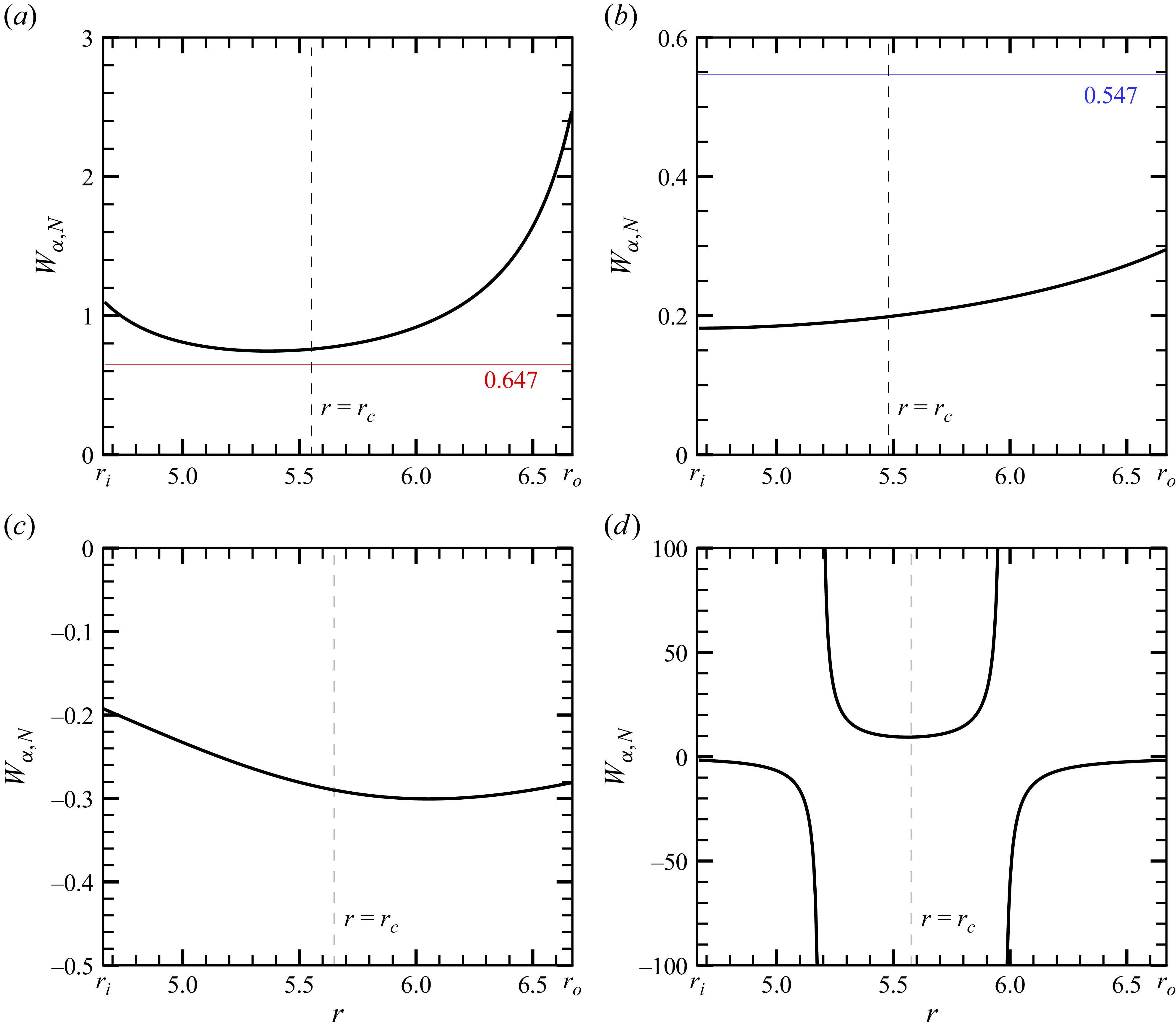


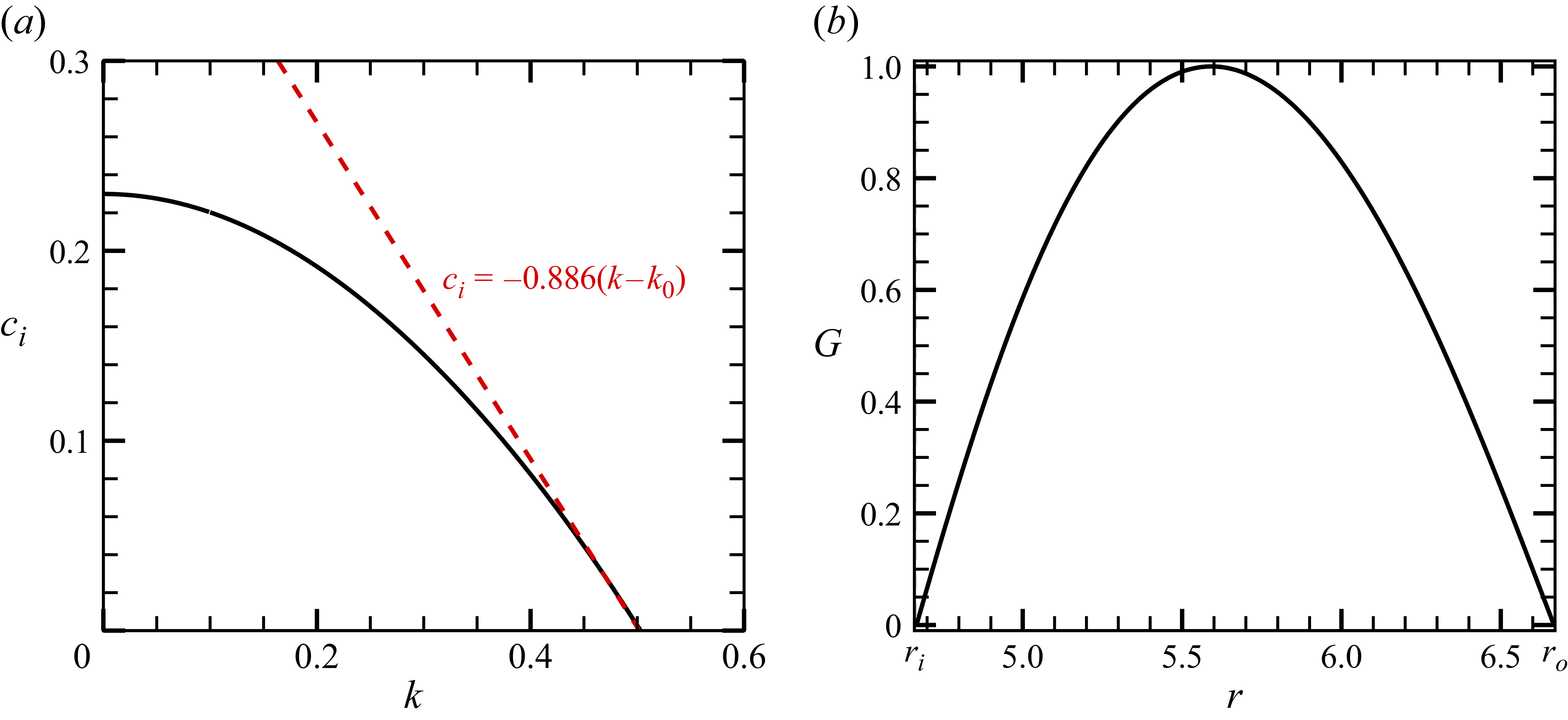


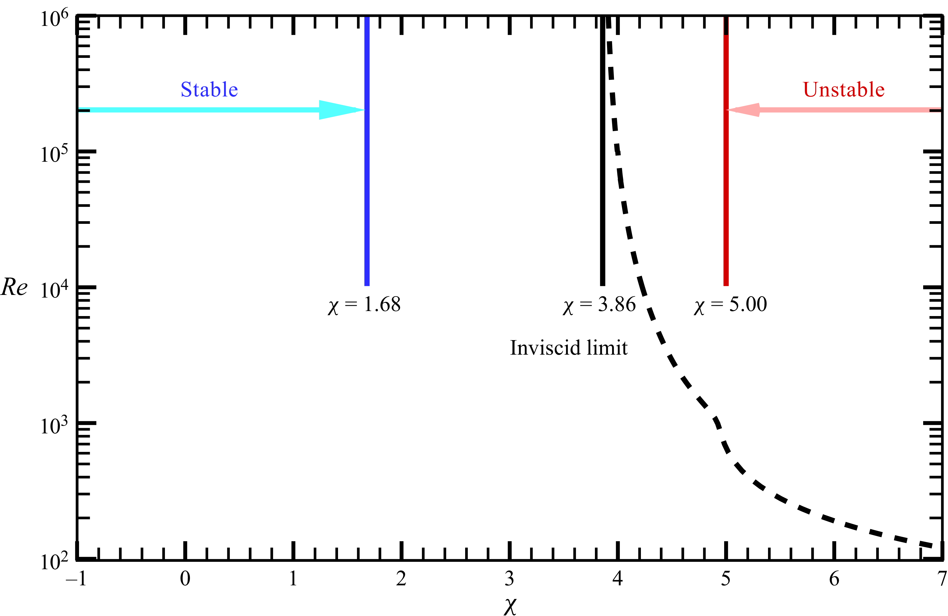





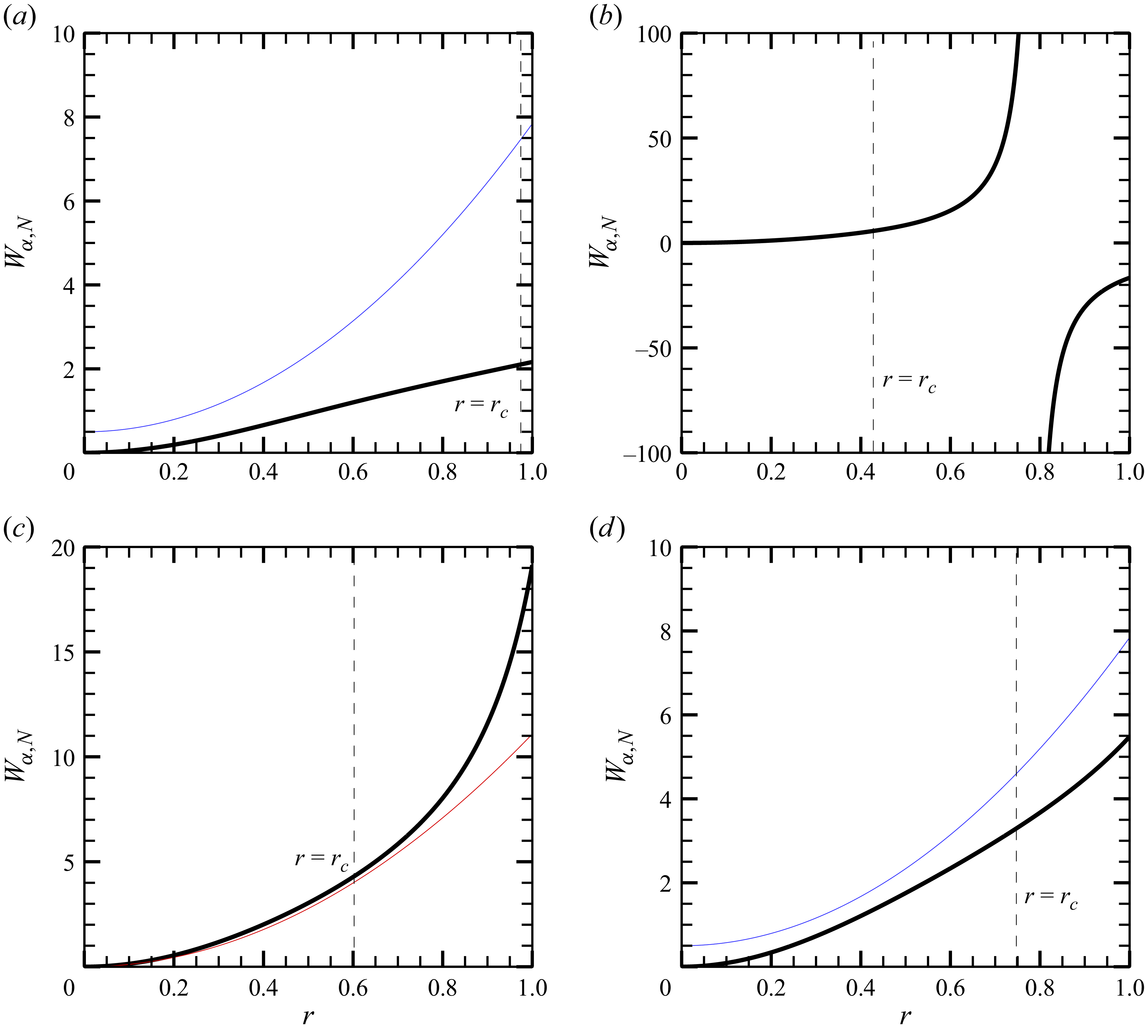


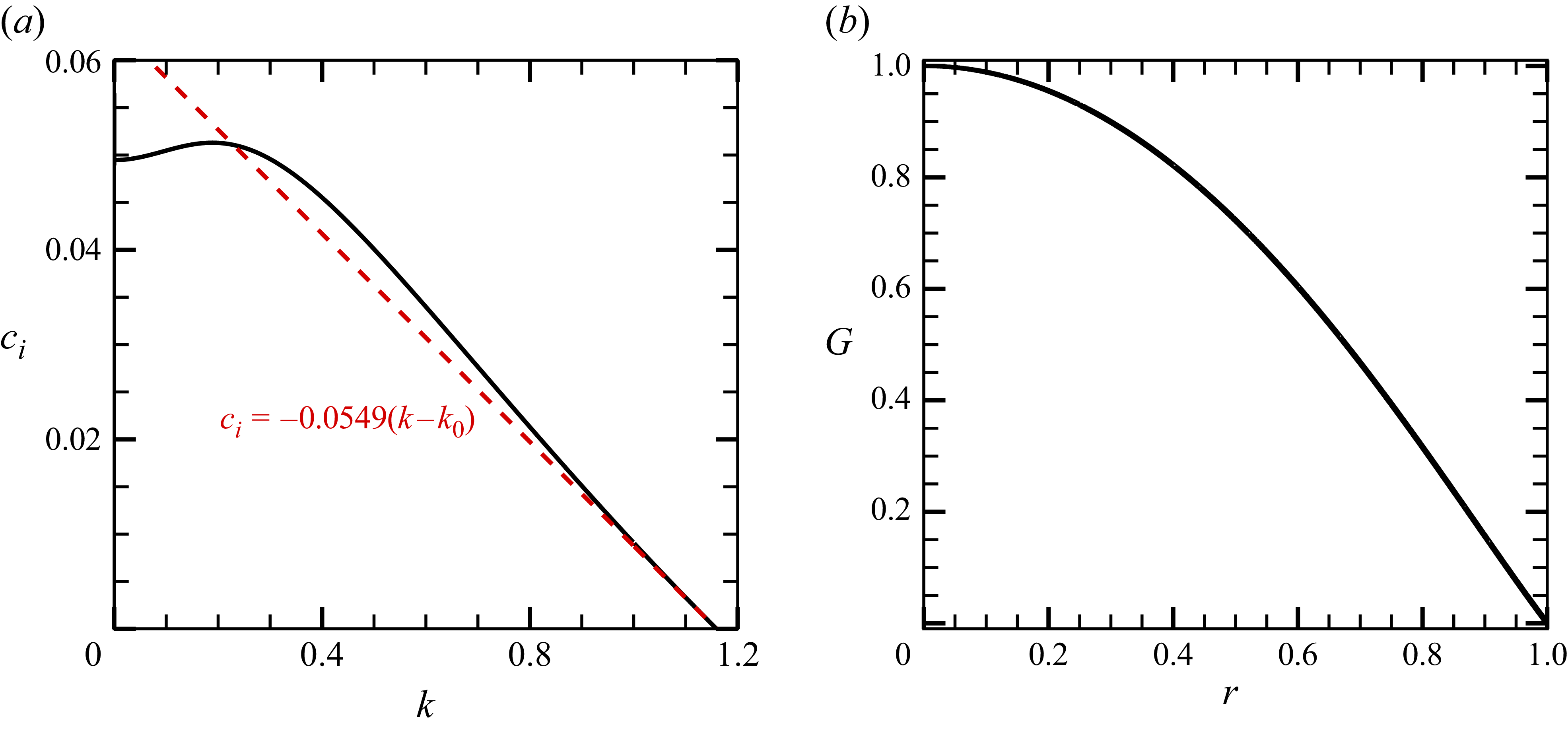


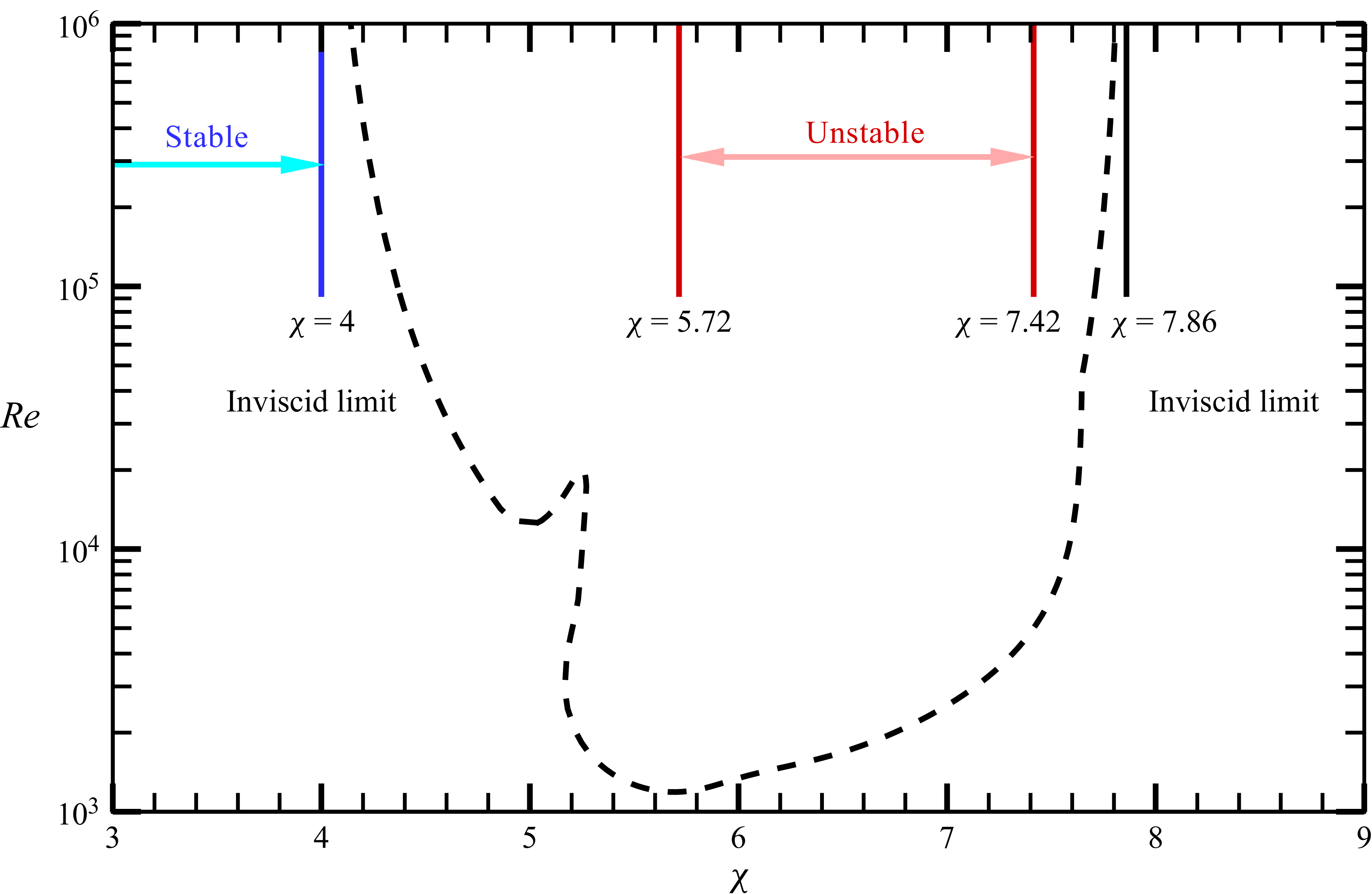

 Open access

