2.1. Experimental facility and operating conditions

The confined bubble swarm was generated within a quasi-bidimensional vertical cell filled with distilled water at ambient temperature, with the top section open to atmospheric pressure (Bouche et al. Reference Bouche, Roig, Risso and Billet2012, Reference Bouche, Roig, Risso and Billet2014). The cell consists of two parallel glass plates ($800$ mm high and $400$ mm wide) separated by a thin gap of width $w = 1$ mm (figure 1a). Unlike in previous works related to confined bubble swarms (Bouche et al. Reference Bouche, Roig, Risso and Billet2012, Reference Bouche, Cazin, Roig and Risso2013, Reference Bouche, Roig, Risso and Billet2014; Alméras et al. Reference Alméras, Cazin, Roig, Risso, Augier and Plais2016, Reference Alméras, Risso, Roig, Plais and Augier2018), no electrolyte was added to the liquid so that bubble coalescence was not inhibited. In addition, the distilled water was regularly renewed to prevent interface contamination. Air bubbles of uniform size were periodically injected from the bottom of the cell through an array of 16 capillary tubes of 0.6 mm inner diameter and 0.8 mm outer diameter (figure 1a). The tubes were equally distributed along the bottom of the cell and connected to a controlled pressure air feeding chamber. The pressure drop along the air injection tubes was sufficiently large to ensure a constant air flow rate along the tubes (Gordillo, Sevilla & Martínez-Bazán Reference Gordillo, Sevilla and Martínez-Bazán2007). The bubble detachment frequency, $f_b$, was accurately selected firstly setting a certain pressure in the air feeding chamber, $p_g$, and, secondly, controlling the air flow rate through each tube using individual valves. This frequency was checked for each injector using a stroboscopic light before running each experiment.

Figure 1.

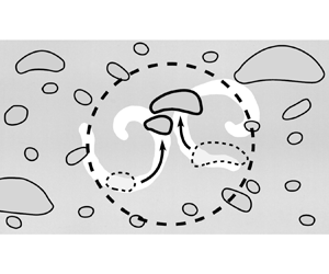
(a) Sketch of the experimental facility, showing the field of view of size $358.40\,{\rm mm} \times 179.20\,{\rm mm}$ for one of the camera recording positions. The zoomed area schematizes the lateral view of the cell with a bubble flattened between the side walls. (b) Example of image taken in one of the three different vertical positions of the camera.

The volume of the injected bubbles ensured that their sizes were always larger than the width of the gap, $w$. Therefore, the bubbles were flattened between the cell walls, forming a thin liquid film between the bubble interface and the wall (see zoomed area in figure 1a). In this configuration, independently of the bubble size distribution of the swarm, no dewetting at the glass plates was observed and the bubbles degrees of freedom were bounded. The flow above the bubbles goes around sideways, and does not enter the thin liquid films at rest as in Pavlov et al. (Reference Pavlov, D'Angelo, Cachile, Roig and Ern2021). Therefore, these thin films are not expected to play any role in the bubble coalescence processes described in the present work. Hence, a two-dimensional description of the motion can be adopted as in Roig et al. (Reference Roig, Roudet, Risso and Billet2012) and Filella et al. (Reference Filella, Ern and Roig2015). In that sense, every bubble in the swarm is described by an equivalent diameter which is defined as $D=(4A_b/{\rm \pi} )^{1/2}$, with $A_b$ the projected area of the bubble on the cell plane. The injected gas volume fraction, $\alpha _0=\varSigma _{i} A^i_b w / (L_x L_z w)$, was determined from the total volume occupied by all the bubbles in a measuring window a few millimetres above the capillary tubes ($W1$ in figure 2), where $L_z=50.83$ mm and $L_x=328.67$ mm are respectively the height and the width of the window. In the current experiments, $\alpha _0$ was varied from $2.4\,\%$ to $6.7\,\%$ by adjusting the bubble generation frequency. Table 1 shows the experimental conditions of the four experimental sets considered in the present work, including the mean equivalent diameter of the injected bubbles, $D_0$. The variations in the sizes of the bubbles generated by each tube was negligible and a monodispersed bubble swarm was initially formed, as in Bouche et al. (Reference Bouche, Roig, Risso and Billet2012, Reference Bouche, Roig, Risso and Billet2014). Additionally, the total air flow rate was estimated as $Q_g = 4 {\rm \pi}{D_0}^2 w f_b$, showing a linear increase with $\alpha _0$.

Figure 2.

General view of the three recording positions for $\alpha _0 = 3.2\,\%$. The 15 measuring windows used for the spatial discretization are superimposed on the images. The height of each measuring window is $L_z = 50.83$ mm while its width almost comprises the whole transverse spanwise of the cell, $L_x = 328.67$ mm. The vertical axis denotes the position of the middle point of some of the measuring windows.

Table 1.

Injection conditions of the four experimental sets considered in the present work: $\alpha _0$, gas volume fraction at the bottom of the cell; $D_0$, mean equivalent diameter of the bubbles injected; $p_g$, pressure at the air feeding chamber; $f_b$, bubble generation frequency; $Q_g$, air flow rate.

The bubble swarm at the bottom of the cell is characterized by $\alpha _0$ and by the non-dimensional parameters governing the motion of an isolated bubble of equivalent diameter at injection, $D_0$. These include the Archimedes number, $Ar_0 = \sqrt {gD_0} D_0 / \nu$, the confinement ratio, $\delta _0 = w / D_0$, and the Bond number $Bo_0 = \rho g D_0^2 / \sigma$, where $g$ is the gravity, $\nu$ and $\rho$ the liquid kinematic viscosity and density, $w$ the thickness of the cell and $\sigma$ the surface tension. Under the conditions reported here, these parameters lie in the following ranges: $630 \leq Ar_0 \leq 850$, $0.24 \leq \delta _0 \leq 0.29$, and $1.79 \leq Bo_0 \leq 2.11$. For confined bubbles of equivalent diameter $D \geq D_0$, the mean rise velocity of an isolated bubble can be estimated by (Filella et al. Reference Filella, Ern and Roig2015)

(2.1)\begin{equation} U_{b} \simeq 0.75(w/D)^{1/6} \sqrt{gD}, \end{equation}

which in dimensionless form can be expressed as,

(2.2)\begin{equation} Re \simeq 0.75 \delta^{1/6} Ar, \end{equation}

where $Re= U_{b}D/\nu$ and $Ar = \sqrt {gD} D / \nu$ are the Reynolds and Archimedes number of a bubble of size $D$. The bubble Reynolds number, $Re_0 = U_{b}D_0/\nu$, can then be defined, and ranges here from $380$ to $500$. The gap Reynolds number, $Re_0{\delta _0}^2$, can then also be introduced to assess the inertial regime, as it varies between $28$ and $32$. Thus, the flow can be considered to be dominated by inertia (Bush & Eames Reference Bush and Eames1998) for all bubble sizes involved in the swarm. Bubbles at injection initially behave as isolated bubbles exhibiting oscillatory paths coupled to their unsteady wakes that generate periodic vortex shedding. Their in-plane projected shape is deformed and can be considered as an ellipse of moderate eccentricity (Roig et al. Reference Roig, Roudet, Risso and Billet2012; Filella et al. Reference Filella, Ern and Roig2015). For further discussion, general ideas can be retained. First, the velocity disturbances induced by bubbles in the liquid are mainly parallel to the plates, except in the close vicinity of the bubbles. Then, the order of magnitude of the liquid velocity in the bubble's wake is $\sqrt {gD}$. The wake is nevertheless strongly attenuated by shear stress at the walls within a characteristic time scale proportional to the viscous one, $\tau _{\nu } = w^2 / (4\nu )$. Therefore, in the swarm the agitation in the liquid results from direct interactions of localized random flow disturbances of various sizes as in the homogeneous swarm studied by Bouche et al. (Reference Bouche, Roig, Risso and Billet2014).

The swarm of bubbles generated was recorded using shadowgraphy in a measurement region that spanned almost the entire horizontal width of the cell (figure 1). To that aim, the cell was illuminated from behind with an uniform, constant and diffused white light perpendicular to the cell plane (figure 1a). Placing the light source at one side of the cell, a camera (Photron APX) equipped with a $85$ mm lens was used to take images of $2^{10}$ levels of grey and of size $1024 \times 512$ pixels, with an exposure time of $1/2000$ s, from the other side. In order to analyse the evolution of the population of bubbles as they rise, while maintaining the desired resolution, the backlight and the camera were placed at three different positions (figure 2). Transverse homogeneity of the flow was observed. Therefore, the downstream evolution of the bubble swarm was described by a statistical analysis of the bubble population characteristic parameters averaged over the horizontal width of the cell. In order to avoid possible errors due to border effects, the analysis was performed in a recording region, placed in the middle of each image, which consisted of a rectangle of size $328.67\,{\rm mm} \times 152.49\,{\rm mm}$ with a pixel-size resolution of $350\,\mathrm {\mu }{\rm m}$ (figure 1b). Moreover, to increase the spatial resolution of the measurements, the recording region was divided into five windows of horizontal length $L_x = 328.67$ mm and vertical length $L_z = 50.83$ mm, with $50\,\%$ of overlapping, as indicated in figure 2. Two types of measurements were performed, depending on the image acquisition frequency. First, a series of experiments taking video images of the swarm at 250 f.p.s. were conducted. This recording rate was high enough to track the bubbles as they rose along the field of view. Thus, bubble collisions could be detected and tracked to determine whether the colliding bubbles coalesced, generating new larger bubbles, or eventually separated, which allowed us to determine the bubble collision frequency, $h$, as well as the efficiency, $\lambda$. Measurements also allowed us to detect breakup events, giving birth to smaller daughter bubbles, although this phenomenon was rare in this study. For this analysis, high-speed movies of 25 s duration were recorded at the three positions. The total duration of the recordings included between $20\,000$ and $75\,000$ bubble records per position, depending on the injection conditions and on the measuring location. In addition to the experiments recorded at high frequency, at each recording position, sets of around 3000 uncorrelated images were recorded at a frame rate of 1/2 f.p.s. to ensure that the bubbles in one image were not recorded in the following one. Thus, the total number of bubbles detected at each position varied between $25\,000$ and $250\,000$, depending on the injected air flow rate and on the recording position. This ensured a statistically converged and unbiased measurement of parameters of the bubble population that can be obtained from low frequency experiments such as the volume probability density function. Satisfactory comparison of the information that could be obtained from both types of measurements indicated that the statistical parameters extracted only from the high-frequency records were indeed robust and meaningful.

Details of the digital image processing methods specifically developed in this work to detect and classify the bubbles in the swarm are given in § A.1. In addition, the techniques designed to track the bubbles and detect the collisions, as well as the coalescence and breakup events are described in § A.2. Additional information can be found in Ruiz-Rus (Reference Ruiz-Rus2019).

2.2. Performance of the bubble tracking algorithm (BTA)

The results obtained with the bubble tracking algorithm (BTA) described in Appendix A, consist of the record of the bubbles along the field of view for each position. The information stored for each bubble includes the projected area (bubble volume), the centroid location, the bubble velocity components, as well as the bubble lifespan and the types of birth and death events. In addition, family trees are established for each newly generated bubble, including the parents in a birth from coalescence, or the mother and the sibling in a birth from breakage. The performance of the BTA algorithm can be estimated, first, from the fact that more than $99 \, \%$ of the detected bubbles can be tracked, the remaining ones being associated to specific events with simultaneous coalescence and breakup in agglomerates of bubbles.

As an example, figure 3 shows a set of bubble trajectories for each injection condition at the first recording position. In this figure, regardless of where the bubble trajectories begin, they have been displaced to the same origin, with $x_o$ and $z_o$ being the initial positions of the bubbles. It can be observed that the horizontal dispersion of the bubbles increases with the injected air volume fraction and with the vertical position, showing the effects of the liquid velocities induced by the wakes of the population of bubbles. The bubble lifespan is typically larger for the lowest values of $\alpha _0$ (figure 3a,b), since the number of coalescence events is still low at this recording position. The trajectories show the characteristic path oscillations described by Roig et al. (Reference Roig, Roudet, Risso and Billet2012) for isolated bubbles, indicating the weak effect of the hydrodynamic interactions at these low void fractions. However, the degree of coalescence substantially increases with $\alpha _0$, resulting in much shorter trajectories (figure 3c,d).

Figure 3.

Superimposed trajectories of 100 bubbles detected in the field of view of the first recording position, $z<160$ mm, for the different injection conditions (a) $\alpha _0 = 2.4\,\%$; (b) $\alpha _0 = 3.2\,\%$; (c) $\alpha _0 = 4.9\,\%$ and (d) $\alpha _0 = 6.7\,\%$. Each trajectory is defined as a succession of points corresponding to the bubble centroid at each instant. The origin ($x_o, z_o$) is defined as the position where the bubble is first detected. The positions are normalized using the corresponding injection diameter $D_0$.

The first quantitative measurement extracted from the BTA is the collision efficiency. It represents the ratio between the number of coalescence and that of collisions. As mentioned before, the confinement of the bubbles imposed in this configuration highly increases the efficiency of the collisions. The mean collision efficiency, $\lambda _\infty$, obtained considering all the collisions detected at each measuring window, is plotted in figure 4 for the four values of $\alpha _0$ tested in this work. Our results indicate that the collision efficiency barely depends on the size of the colliding bubbles. In fact, considering the collision efficiency of different pairs of bubbles, differences lower than $5 \, \%$ were found with respect to $\lambda _\infty$. In addition to being a very high efficiency, it should be noted that $\lambda _\infty$ does not vary with the concentration of bubbles, nor with $z$. In fact, the figure shows that its value can be considered constant and approximately equal to $80 \, \%$.

Figure 4.

Mean collision efficiency of the populations of bubbles, defined as the fraction of collisions that end up in coalescence, vs the downstream distance normalized by the corresponding injection diameter $D_0$. The figure shows that $\lambda _\infty$ remains constant and does not depend on $\alpha _0$.

Moreover, the tracking method allows a direct analysis of the coalescence events. In that sense, any detected collision is individually tracked (see § A.2), obtaining the position at which it initially occurs as well as the corresponding information for the colliding bubbles. In addition, the BTA can be used to obtain the number of bubbles of volume $v$ that die due to coalescence, and the mean coalescence frequency of all bubbles at each position,

(2.3)\begin{equation} {\langle g_c \rangle}_\infty= \frac{\int^{\infty}_{0} n(v) g_c(v) \,{\rm d}v}{\int^{\infty}_{0} n(v)\, {\rm d}v}, \end{equation}

that represents the frequency at which a bubble of any size coalesces with other bubbles. In the experiments performed in this work, most of the daughter bubbles which are born due to coalescence come from previous binary collisions. Thus, since the total number of collisions which end up in coalescence, $\gamma _\infty$, during the measuring time, $T$, in a population of $N_\infty$ bubbles, is half of the bubbles dying due to coalescence, $N_\infty {\langle g_c \rangle }_\infty /2$, the mean bubble coalescence frequency can be directly obtained from the experimental measurements as

(2.4)\begin{equation} {\langle g_c \rangle}_\infty = \frac{2\gamma_\infty}{N_\infty \; T}. \end{equation}

Similar to the mean coalescence frequency, ${\langle g_c \rangle }_\infty$, the mean breakup frequency of bubbles at each position, given by ${\langle g_b \rangle }_\infty = \int ^{\infty }_{0} n(v) g_b(v)\,{\rm d}v/ \int ^{\infty }_{0} n(v)\,{\rm d}v$, can be directly obtained as

(2.5)\begin{equation} {\langle g_b \rangle}_\infty = \frac{\psi_\infty}{N_\infty \; T}, \end{equation}

where $\psi _\infty$ is the number of breakup events observed during the time $T$.

Thus, the accuracy and convergence of the tracking analysis of the experiments performed at high rates of acquisition can be checked by comparing both sides of (1.2) averaged over all bubble sizes, assuming that both coalescence and breakup are binary processes. To that aim, the right-hand side of the averaged PBE can be achieved by integration of (1.2) over the whole range of bubbles (Friedlander Reference Friedlander1977). Thus, applying the Leibnitz rule for integration and substituting (1.5) and (1.6) into (1.2), in the one-dimensional, steady state situation of interest here, the averaged PBE simplifies to (Kocamustafaogullari & Ishii Reference Kocamustafaogullari and Ishii1995; Soligo, Roccon & Soldati Reference Soligo, Roccon and Soldati2019)

(2.6)\begin{equation} - \frac{1}{N_\infty} \frac{\partial (N_\infty \bar{U}_z)}{\partial z} = \frac{{\langle g_c \rangle}_\infty}{2} - {\langle g_b \rangle}_\infty, \end{equation}

where $\bar {U}_z$ is the mean rising velocity of the bubbles in the measuring window. Figure 5 shows the different terms on both sides of (2.6), evaluated at various measuring locations, for all the experimental injection conditions. In that case, the frequency terms have been made dimensionless making use of $\sqrt {g/D_0}$, while the downstream locations are normalized with the injection diameter $D_0$, corresponding to each experimental injection condition. As expected, a fairly good agreement is observed between both sides of the equation (black circles and grey diamonds, respectively). This result confirms the validity of the experimental procedure, as well as the effectiveness of the bubble tracking method and the convergence of the results obtained. In addition, it can be noticed that some breakup events (hollow squares) also take place in the swarm, especially for the higher values of $\alpha _0$ (figure 5c,d).

Figure 5.

Downstream evolution of the different rates of change of the whole population of bubbles for different injection conditions, (a) $\alpha _0 = 2.4\,\%$; (b) $\alpha _0 = 3.2\,\%$; (c) $\alpha _0 = 4.9\,\%$ and (d) $\alpha _0 = 6.7\,\%$. All these frequency terms have been made dimensionless with $\sqrt {g/D_0}$. Both sides of the averaged PBE, as expressed in (2.6), are shown with solid symbols, left-hand side (diamonds) and right-hand side (circles). In addition, the different rate of change terms on the right-hand side of (2.6) are represented with open symbols, half of the mean coalescence frequency (triangles) and the mean breakup frequency (squares).

3.1. Spatial evolution of the bubble population

In the present configuration there is no external liquid flow that carries the bubbles and they rise due to buoyancy effects. The downstream evolution of the population of bubbles can be described in terms of the flux of bubbles crossing each $z$ position. An estimation of the averaged flux is given by the local net number of bubbles detected in each measuring window, $N^*_\infty$, multiplied by their corresponding mean velocity, $\bar {U}_z$, obtained by the BTA. Figure 6(a) shows the downstream evolution of the bubbles flux for each injection condition. The fact that the flux of bubbles decreases with the dimensionless downstream location $z/D_0$, indicates that coalescence leads the evolution of the distribution of bubbles, even in the cases where there are some breakup events, as previously shown in figure 5. The rate of change of the population depends on the initial number of bubbles, $N^*_\infty (0)$, which is directly related to the selected bubble generation frequency, $f_b$, and thus, to the injected air volume fraction, $\alpha _0$. For high void fractions (i.e. $\alpha _0 = 4.9$ and $6.7\,\%$, respectively), near the bottom of the cell, the amount of bubbles of injection size $D_0$ quickly decreases as the bubbles rise. In fact, strong bubble–bubble interactions occur in the regions close to the injectors, giving rise to collisions and coalescence events. Once the bubbles start coalescing, larger bubbles are generated leading to a coalescence cascade which rapidly involve pairs of bubbles of wider ranges of sizes. As $z/D_0$ increases, the flux decreases less rapidly. In fact, the reduction in the total number of bubbles composing the population causes the net amount of coalescence events to decrease too. Although the rate of change of the bubbles flux decreases with the downstream distance, there is no evidence of reaching a final frozen state where coalescence would become negligible. It has to be pointed out that at higher positions of the cell, as previously noticed in figure 5(c,d), bubble breakup occurs, competing with coalescence. The unstable nature of the largest bubbles generated in these cases as well as the interaction with stronger bubble-induced liquid velocities, increases the relevance of breakage far from the injection point. On the other hand, for lower void fractions (i.e. $\alpha _0 = 2.4\,\%$ and $3.2\,\%$), figure 6(a) shows that the bubbles take longer to begin to coalesce. In these cases, the bubble flux initially remains constant up to a certain position where it starts to decay at a rate that decreases as $\alpha _0$ decreases. This is related with the lower amount of bubbles generated under these conditions and the larger distances between bubbles at the initial positions. However, as they rise, the injected bubbles loose memory of the injection conditions and begin to adopt the oscillatory motion which characterizes these ellipsoidal bubbles within the confined cell (Roig et al. Reference Roig, Roudet, Risso and Billet2012; Filella et al. Reference Filella, Ern and Roig2015). At a given height that depends on the generation frequency (Sanada et al. Reference Sanada, Watanabe, Fukano and Kariyasaki2005), the trajectories of the bubbles scatter under the effect of the perturbations in the liquid, giving rise to bubble–bubble interactions and to the subsequent collisions and coalescence events (see $W4$ and $W5$ in figure 2).

Figure 6.

(a) Downstream evolution of the total flux of bubbles measured in each position (window) for the different experimental injection conditions. (b) Downstream evolution of the local gas volume fraction, obtained from the total volume occupied by all the bubbles present in each window. The downstream locations have been normalized by the corresponding injection diameter $D_0$.

Figure 6(b) shows, for each injection condition, the downstream evolution of the local air volume fraction $\alpha (z)$, defined as the volume occupied by the entire population of bubbles present at each measuring window, divided by the volume of the window. At variance with homogeneous monodispersed bubble swarms where the gas volume fraction remains constant under constant injection conditions (Martinez Mercado et al. Reference Martinez Mercado, Chehata, Van Gils, Sun and Lohse2010; Bouche et al. Reference Bouche, Roig, Risso and Billet2012; Colombet et al. Reference Colombet, Legendre, Risso, Cockx and Guiraud2015), in the present swarm, $\alpha (z)$ also varies with $z/D_0$, due to the evolution of the distribution of sizes and to the fact that the velocity of the bubbles varies with their sizes. Indeed, the absence of an external liquid flow implies that the mean rising velocity of the gas phase is mainly imposed by the buoyancy exerted on the different bubble sizes coupled to the underlying fluid motion generated by hydrodynamic interactions. Therefore, the local volume fraction $\alpha (z)$ is affected not only by the injected air flow rate, but also by the evolution of the distribution of bubbles that induces buoyancy-driven variations on the mean rising velocity of the gas phase.

In order to determine the distribution of bubble sizes at each measuring window, the equivalent diameters of the bubbles were obtained from image processing (see § A.1) to compute the bubble volume probability density function (v.p.d.f.) (Martínez-Bazán et al. Reference Martínez-Bazán, Montañés and Lasheras1999a),

(3.1)\begin{equation} \mathrm{V.p.d.f.}\, (D) = \dfrac{ w D^2 \mathrm{p.d.f.}\,(D)}{\displaystyle \int_{D_{min}}^{D_{max}} w D^2 \, \mathrm{p.d.f.}\,(D) \, \mathrm{d}D } , \end{equation}

which represents the volume occupied by bubbles of size $D$ compared with that of the entire distribution. In (3.1), $D_{min}$ is the smallest bubble size of the distribution and $D_{max}$ the largest one. The downstream evolution of the v.p.d.f. resulting from coalescence, and eventually breakup, is shown in figure 7 for the four experimental conditions reported in table 1. For the sake of clarity, we have only plotted six measuring locations. Qualitatively, similar downstream evolutions are observed for the four cases: the nearly monodispersed distribution of bubbles observed close to the bottom of the cell progressively widens further downstream due to bubble coalescence. Since bubbles of constant size, $D_0$, are periodically injected at the bottom of the cell, for low values of $\alpha _0$, the initial v.p.d.f. is a narrow distribution around $D_0$ (see the distribution at $z = 40.92$ mm in figure 7a,b). In fact, in these cases, coalescence is not observed until $z = 142.58$ mm (figure 7a,b), as previously noted from the evolution of the total flux of bubbles shown in figure 6(a). However, for larger values of $\alpha _0$, at the first measuring window, a secondary peak is already observed at $D \simeq \sqrt {2}D_0$, indicating the existence of some coalescence events of bubbles of size $D_0$ ($z = 40.92$ mm in figure 7c,d). It is worth noting the existence of additional peaks at $\sqrt {3}D_0, \sqrt {4}D_0, \ldots$, corresponding to added volumes of the injection bubbles resulting from successive coalescence events (Néel & Deike Reference Néel and Deike2021). Nevertheless, as the coalescence process evolves, such peaks (associated with classes of finite extension) attenuate, generating broader and smoother distributions far from the injection point. The v.p.d.f.s exhibit large tails as the coalescence cascade progresses. In fact, it can be observed that the size of the largest bubbles found at a certain distance increases with $\alpha _0$. This fact is clearly illustrated in the images displayed as insets in figure 7, which show characteristic snapshots of the swarm for each experimental condition at $z = 412.92$ mm.

Figure 7.

Downstream development of the bubble size distribution described by the volume-size bubble p.d.f. for (a) $\alpha _0 = 2.4\,\%$, (b) $\alpha _0 = 3.2\,\%$, (c) $\alpha _0 = 4.9\,\%$ and (d) $\alpha _0 = 6.7\,\%$. Only some measuring locations have been plotted for clarity. The image inside each panel corresponds to a cell height around $z = 412.92$ mm. The scale bar indicates a length of 20 mm.

For all values of $\alpha _0$, despite the differences in the downstream evolution of the rate of change of the number of bubbles, similar shapes of the distribution are found at different positions, which can be understood as equivalent stages of the coalescence cascade process. For example, the distribution at $z=324.58$ mm in figure 7(a) is similar to that at $z=222.92$ mm in figure 7(b), the distribution at $z=324.58$ mm in figure 7(b) matches that at $z=142.58$ mm in figure 7(c) and the distribution at $z=514.58$ mm in figure 7(c) resembles that at $z=412.92$ mm in figure 7(d). The similarity in the distribution evolutions reveals that the various swarms considered follow the same coalescence cascade, independently of the value of $\alpha _0$. However, the rate of change of the swarm strongly depends on the void fraction, which is directly related to the amount of bubbles forming the population, as can be inferred from (1.5). It will take longer for low values of $\alpha _0$ (figure 7a,b) than for larger ones (figure 7c,d) to reach a given stage of the distribution of sizes (i.e. a given shape), although each size will undergo the same coalescence cascade independently of $\alpha _0$. Taking this into account, the evolution of the bubble size distribution is characterized by a diameter representative of the population of bubbles. For this purpose, we used the statistically robust parameter, $D_{V90}$ (Hinze Reference Hinze1955; Martínez-Bazán, Montañés & Lasheras Reference Martínez-Bazán, Montañés and Lasheras1999b), defined as the diameter of a bubble such that 90 % of the total volume of the population of bubbles is contained within bubbles smaller than $D_{V90}$. This characteristic diameter represents the size of the largest bubbles in the distribution which, as they rise, will induce the largest velocity fluctuations in the liquid.

Figure 8(a) shows the downstream evolution of $D_{V90}$ for the four injection conditions, reflecting the increase of its rate of change with $\alpha _0$. Note that, for $\alpha _0= 2.4\,\%$ and $3.2\,\%$, $D_{V90}$ barely changes for $z< 150$ mm, indicating that coalescence does not start in those cases until $z > 150$ mm. However, for $\alpha _0= 4.9\,\%$ and $6.7\,\%$, coalescence is already observed near the injection position. In addition, figure 8(b) shows the evolution of the flux of bubbles normalized by that of the first measuring window, $N^*_{\infty } \bar {U}_z(0)$, as a function of the characteristic diameter $D_{V90}$ normalized by the diameter of the injected bubbles, $D_0$. It can be observed that the four plots collapse on the same curve, corroborating that the population of bubbles follow similar coalescence cascade processes and that $D_{V90}$ is the proper variable to describe the evolution of the population of bubbles of the different swarms. In that sense, $D_{V90}/D_0$ can be seen as a variable similar to the dimensionless time, $t/\tau$, proposed by Smoluchowski (Reference Smoluchowski1917) to describe the Brownian coagulation of particles within nearly monodispersed systems (see Chandrasekhar Reference Chandrasekhar1943; Friedlander Reference Friedlander1977, for reports of this work in English), being $\tau$ the characteristic coagulation or decay time, usually called half-life of the population. So, in the following, $D_{V90}$ will be considered as the characteristic parameter to determine the evolution of the swarm. This will allow us to consider the coalescence frequency as an unknown that varies with the self-induced evolution of the population, which includes the influence of the a priori unknown velocities of each size, as well as the $\alpha _0$ dependence.

Figure 8.

(a) Evolution of $D_{V90}$ with the downstream location, both normalized with the corresponding bubble injection diameter $D_0$, for the different injection conditions. Note that $D_{V90}/D_0$ remains unchanged until the coalescence process starts, leading to larger bubbles. (b) Evolution of the flux of bubbles normalized with that at the first measuring window, $N^*_{\infty } \bar {U}_z(0)$, as a function of $D_{V90}/D_0$.

As already indicated above, the aim of the present work is to experimentally determine the coalescence frequency of a pair of bubbles of sizes $D$ and $D'$, respectively, in the bubble swarm. To be able to do this, large enough size ranges have to be defined to ensure that the number of bubbles included in each range is sufficiently high to have an adequate number of colliding bubbles and, thus, obtain statistically converged results. For this purpose, we discretized the population of bubbles obtained from the experiments in different size classes, denoted as class 0, 1, 2 and so on. Every class is represented by a diameter $D_k$ and includes bubble sizes in the range $D_k -\varDelta _k/2$ $\le D \le$ $D_k +\varDelta _k/2$, within a size bin of width $\varDelta _k$. The diameter $D_k$ represents the middle size of the bin and corresponds to integer values of the injection bubble volume, accounting for volume-conservative coalescence events. Thus, the initial class corresponds to the injection bubbles, $D_0$. The following class is associated to the coalescence of two bubbles of size $D_0$, being $D_1^2 = 2D_0^2$. The rest of the classes, $D_k$, are defined as the diameter of the bubble formed from the coalescence of two bubbles belonging to the two preceding classes, $D_k^2 = D^2_{k-1} + D^2_{k-2}$. Therefore, the different classes represent added volumes of the injection bubbles resulting in the following diameters: $D_1=\sqrt {2} D_0$, $D_2=\sqrt {3} D_0$, $D_3=\sqrt {5} D_0$, $D_4=\sqrt {8} D_0$, $D_5=\sqrt {13} D_0$, $D_6=\sqrt {21} D_0$, $D_7=\sqrt {34} D_0$ and $D_8=\sqrt {55} D_0$. The different sizes of the bins, $\varDelta _k$, were chosen looking for substantial but smooth variations of the bubble characteristics. Such definition of bubble classes and their corresponding limits allowed us to have an amount of bubbles sufficiently large in each class to observe enough collision events among bubbles of different classes, ensuring a good statistical convergence of the data. Details of the bubble classes defined for the different injection conditions are listed in table 2.

Table 2.

Description of the bubble size classes defined for each experimental set. Here, $k$ denotes the bubble class indicating the symbols used to represent them, $D_k$ is the mean diameter describing the class and $\varDelta _k$ the width of the size bin containing the class.

Considering the bubble classes defined in table 2, the number of bubbles of a certain class per unit volume, $N_k$, is obtained by integrating (1.3) between the size limits of the corresponding bin, $D_k -\varDelta _k/2$ and $D_k +\varDelta _k/2$. The evolution of the fraction of bubbles of each class, $N_k / N_{\infty }$, is represented in figure 9, as a function of $D_{V90} / D_0$ for $\alpha _0= 6.7\,\%$, showing the contribution of the amount of bubbles of each class to the whole population in every stage of the coalescence process. Note that, as shown in the inset of figure 9, the fraction of injection bubbles (class $k=0$) is always larger than those of the other classes, indicating that there is still a considerable amount of bubbles of size $D_0$ remaining even far from the injection point. This fact reveals the appreciable presence of these small bubbles even at stages in which the coalescence cascade has accounted nearly $8^2$ events. After a rapid decrease during the early stages of the evolution, the fraction of injection bubbles almost stabilizes around half of the total number of bubbles. However, the evolution of the fraction of all the other classes remarkably differs from that of the initial bubbles. In fact, a certain class of bubbles does not begin to form until a pair of smaller bubbles, whose sum of volumes is equal to the volume of the forming bubble, coalesce. First, the number of bubbles of classes $k>0$ increases due to coalescence of smaller bubbles. Afterwards, when the number of bubbles of a given class becomes sufficiently large, they start to coalesce forming larger bubbles. Eventually, when the number of coalescing bubbles of a class $k$ is larger than the number of bubbles that are generated from the coalescence of smaller ones, $N_k/N_\infty$ decreases. Indeed, the evolution of the concentration of a certain bubble class within the swarm is driven by the balance between the coalescence rate of smaller bubbles that form bubbles of this class, and their rate of coalescence with all the others, as is clearly established by (1.5). The coalescence rate in the balance equation (1.8) is determined from the collision frequencies of pairs of bubbles, $h(D_k,D_{k'})$, whose experimental values will be obtained in § 3.2 and modelled in § 4.

Figure 9.

Evolution of the fraction of bubbles of each class with $D_{V90}/D_0$ for $\alpha _0 = 6.7\,\%$. Similar values are obtained for the other injection conditions. The fraction of bubbles belonging to the injection class is displayed in the inset for clarity. The symbols represent the different bubble classes according to table 2.

3.2. Determination and analysis of the bubble pair collision frequency, $h(D_k, D_{k'}$)

Considering the discretization in bubble classes given in table 2, the number of bubbles per unit volume of a given class $k$ that die per unit time due to coalescence represents the coalescence death rate, commonly expressed as

(3.2)\begin{equation} \dot D_{ec}(D_k) ={-} \int^{\infty}_{0} \lambda (D_k, D_{k'}) h (D_k, D_{k'}) n(D_k) n(D_{k'}) \, \mathrm{d}D_{k'}={-}g_c(D_k) n(D_k). \end{equation}

In (3.2), $h(D_k, D_{k'})$ is the collision frequency of bubbles of class $D_k$ with bubbles of size $D_{k'}$ and has units of ${\rm m}^3 \,{\rm s}^{-1}$, and $n(D_k)$ is the number density of bubbles with units of ${\rm m}^{-3}$, thus, $\dot D_{ec}(D_k)$ has units of ${\rm m}^{-3}\,{\rm s}^{-1}$. Note that, since $\lambda (D_k, D_{k'})=\lambda _\infty$ is constant in the present case, $h(D_k, D_{k'})$ can be treated indistinctly as the collision or the coalescence frequency of the pair of bubbles. Having this in mind, $h(D_k, D_{k'})$ was obtained from the experiments performed at high acquisition rates, applying the bubble tracking and coalescence detection algorithm described in Appendix A, as

(3.3)\begin{equation} h(D_k, D_{k'})=\frac{\varGamma_{kk'} }{N_k N_{k'}}. \end{equation}

In (3.3), $\varGamma _{kk'}$ is the number of bubbles of class $k$ colliding with bubbles of class $k'$ in the measuring window, of volume $L_z \times L_x \times w$ (see figure 2), per unit time, and $N_k$ and $N_{k'}$ are respectively the number of bubbles of class $k$ and $k'$ accounted in the volume of the measuring window. Thus, the rate of loss of bubbles of class $k$, $\dot D_{ec}(D_k)$, corresponds to the frequency at which effective collisions of bubbles of size $D_k$ with the rest of the bubbles take place, which, assuming that $\lambda (D_k, D_{k'})=\lambda _\infty$ is constant (see figure 4), reduces to ${\dot D_{ec}(D_k)=\lambda _{\infty }}\varSigma {_{k'=0}^{\infty } \varGamma _{kk'}}$. Note that, considering all the bubbles of the distribution which collide per unit time, $\varGamma _\infty =\varSigma _{k=0}^{\infty }\varSigma _{k'=0}^{\infty } \varGamma _{kk'}$, the total number of coalescence events in expression (2.4), can also be obtained as $\gamma _\infty / T = \lambda _\infty \varGamma _\infty /2$. It is worth indicating that the models for $h$ have been commonly derived by making an analogy with the kinetic theory of gases (Vincenti & Kruger Reference Vincenti and Kruger1965). These models (see, e.g. the review in Liao & Lucas Reference Liao and Lucas2010) generally consider $h$ as the volume swept per unit time by the colliding bubbles. It is usually referred to as the collision kernel, or the coalescence kernel if the efficiency is also included (Marchisio & Fox Reference Marchisio and Fox2013). However, taking into account that $h$ is symmetric, resulting in $h(D_k, D_{k'}) = h(D_{k'}, D_k)$, in the present work it will be referred to as the bubble pair collision frequency.

The evolution of $h(D_k, D_{k'})$ is described hereafter for the experimental case corresponding to $\alpha _0 = 4.9\,\%$, as a representative example. Figure 10 shows the results of the bubble pair collision frequency for various bubble pairs at a stage of the evolution of the swarm where $D_{V90} = 18.25$ mm ($D_{V90}/D_0 = 4.74$). The adopted representation displays the evolution of $h(D_k,D_{k'})$ with $D_{k'}$ for the different classes of bubbles (constant values of $D_k$). We should remember that, according to figure 8, since the bubble size distributions evolve in a similar way for all values of $\alpha _0$, $D_{V90}/D_0$ can be used as a parameter to describe the coalescence cascade process. Considering the results corresponding to the smallest bubble size present in the distribution, $D_k = 3.85$ mm ($\CIRCLE$), a monotonous increment of the collision frequency is observed when the size of the other colliding bubble, $D_{k'}$, increases. This behaviour is also initially observed for larger bubbles, i.e. larger values of $D_k$, up to a certain value of $D_{k'}$ beyond which the frequency begins to decrease. Taking into account the interchangeability of $D_k$ and $D_{k'}$, it can be stated that the slope of the curve $h(D_k, D_{k'})-D_{k'}$ increases with $D_k$. This monotonically increasing behaviour of the bubble pair collision frequency, characterized by the fact that at least one of the bubbles involved in the collision is relatively small, will be referred to as the first regime (represented by solid symbols in figure 10). In this regime, as soon as the bubbles collide, they coalesce or (in a very few cases) bounce back, but their surfaces do not deform during a certain time until they coalesce. On the other hand, as observed for $D_k \geq 8.62$ mm ($\blacksquare, \blacktriangledown, \blacklozenge$), the evolution of the bubble pair collision frequency shows a local maximum at certain values of $D_{k'}$, which decreases as $D_k$ increases. After this maximum a different behaviour appears, which defines a second collision/coalescence regime (represented by hollow symbols in figure 10), where the two involved bubbles are large enough to be able to deform during the coalescence process. In this regime, once the bubbles get in touch, their interfaces deform and flatten forming a thin liquid film between the two bubbles, which mainly drains sideways (Huisman et al. Reference Huisman, Ern and Roig2012; Pavlov et al. Reference Pavlov, D'Angelo, Cachile, Roig and Ern2021). The time spent on the bubbles surface deformation and on the liquid film drainage, before coalescence, increases the time during which the bubbles interact, leading to a reduction of the corresponding collision/coalescence frequency.

Figure 10.

Experimental measurements of the bubble pair collision frequency, $h(D_k,D_{k'})$, obtained for the injection condition $\alpha _0 = 4.9\,\%$ at a stage of the evolution of the swarm where $D_{V90} = 18.25$ mm ($D_{V90}/D_0 = 4.74$). The symbols represent the different bubble classes according to table 2. Solid symbols represent pairs of bubbles colliding in the first regime, while hollow ones denote collisions within the second regime. The series corresponding to $D_k = 6.67$ mm and $D_k = 10.90$ mm are not plotted for clarity. The points indicated by arrows correspond to the cases shown in figure 13.

Figure 11(a–d) shows the contours of $h(D_k, D_{k'})$ at four different instants of the coalescence cascade process corresponding to $\alpha _0=$ 4.9 %. In this case, bubbles of diameter $D_0 = 3.85$ mm are initially injected and, as they coalesce while they rise, a population of bubbles of increasing diameters is generated. The values of $D_{V90}$ of the bubble size distributions corresponding to panels (a–d), indicated with horizontal and vertical dashed lines, are 10.93 mm, 13.96 mm, 18.25 mm and 20.79 mm, respectively ($D_{V90}/D_0 = 2.84$; $3.62$; $4.74$ and $5.40$). The plots clearly show that $h(D_k, D_{k'})$ is a symmetric function that increases with $D_{V90}$. In fact, it can be observed that the coalescence frequencies between two small or two large bubbles are small compared with the collision frequency between bubbles of intermediate sizes. Note, for instance, that the maximum coalescence frequency in figure 11(d) falls in a fringe corresponding to the coalescence of bubbles of $D_k=8$ mm ($D_k=20$ mm) with bubbles of $D_{k'}= 20$ mm ($D_{k'}= 8$ mm), or to the coalescence between two bubbles of diameter $D_k=D_{k'} \approx 12$ mm. Interestingly, a close inspection of the contour plots indicates that the colour levels nearly follow lines of constant values of

(3.4)\begin{equation} D_p = \left[\frac{1}{2}\left(\frac{1}{D_k}+\frac{1}{D_{k'}}\right)\right]^{{-}1}=\frac{2 D_k D_{k'}}{D_k + D_{k'}}, \end{equation}

drawn with solid lines in figure 11(a–d). The diameter $D_p$ represents the diameter of a bubble whose radius of curvature is equal to the mean radius of curvature of the pair of interacting bubbles, and will be further called the reduced diameter. This diameter has been commonly used to describe the deformation of interacting bubbles and in models of drops/bubbles coalescence (Chesters & Hofman Reference Chesters and Hofman1982; Kamp et al. Reference Kamp, Chesters, Colin and Fabre2001; Neitzel & Dell'Aversana Reference Neitzel and Dell'Aversana2002). In addition to $h(D_k, D_{k'})$ shown in figure 11(a–d), figure 11(e–h) displays the bubble pair collision frequency weighted by the number of bubbles of size $D_{k'}$. This quantity represents the frequency of collision of a bubble of size $D_k$ with bubbles of size $D_{k'}$ and obviously depends on the number of bubbles of size $D_{k'}$ in the distribution, $n(D_{k'})$. It represents the contribution of bubbles of class $k'$ to the coalescence frequency of bubbles of class $k$, $g_c(D_k)$, as established in (1.7). It can be seen that $h(D_k, D_{k'}) N_{k'}$, obtained experimentally as $\varGamma _{kk'}/ N_k$ is no longer symmetric and it depends on the bubbles size distribution, having the maximum values for $D_{k'}=D_0$ in our particular case, since the number of bubbles of size $D_0$ is larger than the number of bubbles of other sizes, as shown in figure 9.

Figure 11.

Contour plots of: (a–d) $h(D_k, D_{k'})$ and (e–h) the product $h(D_k, D_{k'}) N_{k'}$ for $\alpha _0 = 4.9\,\%$ at four different instants of the bubble coalescence cascade process, characterized by $D_{V90}$ (indicated by dashed lines in each plot). Results are shown for (a,e) $D_{V90} = 10.93$ mm ($D_{V90}/D_0 = 2.84$); (b,f) $D_{V90} = 13.96$ mm ($D_{V90}/D_0 = 3.62$); (c,g) $D_{V90} = 18.25$ mm ($D_{V90}/D_0 = 4.74$) and (d,h) $D_{V90} = 20.79$ mm ($D_{V90}/D_0 = 5.40$). The solid black lines in (a–d) indicate constant values of the reduced diameter $D_p$.

A description of the bubble pair collision frequency, $h(D_k,D_{k'})$, is therefore sought after in terms of the reduced diameter, $D_p$. The experimental values of $h(D_k,D_{k'})$ displayed in figure 10 are represented as a function of the corresponding $D_p$ in figure 12(a). They fall on a single curve, represented by the thick solid line, which corresponds to the averaged bubble pair collision frequency along lines of constant $D_p$ in figure 11(c). This curve clearly indicates the existence of the two different collision regimes commented above, properly distinguished now as a function of $D_p$. Initially, in the first regime (solid symbols), $h(D_p)$ increases with $D_p$ until it reaches a maximum value beyond which it begins to decrease with $D_p$ (hollow symbols). In this figure, as in figure 10, the cases indicated by arrows correspond to the time series of experimental images shown in figure 13. Equivalent results are found for different values of $D_{V90}$, as shown in figure 12(a) (different lines) for the instants of the coalescence cascade presented in figure 11(a–d). This result corroborates that $D_p$ properly captures the dependence of the collision frequency on the bubble sizes. The values of the reduced diameter at which the maximum of $h(D_p)$ occurs, i.e. the change from the first to the second collision regime, denoted as $\tilde {D}_p$, are displayed in figure 12(b) for the different experimental cases tested. For the smallest value of the injected volume fraction, $\alpha _0 = 2.4\,\%$, the entire coalescence cascade took place in the first regime, without transitioning to the second one, and no data are represented in this case. It can be observed that $\tilde {D}_p$ increases with the concentration of bubbles and with $D_{V90}$, following a power law given by $\tilde {D}_p/w\propto (\alpha D_{V90}/w)^{1/2}$ as it will be commented later on in § 4.

Figure 12.

(a) Bubble pair collision frequency, $h(D_k,D_{k'})$, as a function of the reduced diameter, $D_p$. The symbols represent the experimental results shown in figure 10. Collisions taking place in the first regime are depicted with solid symbols, while hollow ones are used to represent collisions in the second regime. As in figure 10, the cases labelled as (i), (ii) and (iii), respectively, correspond to the series (a–c) in figure 13. Lines represent the averaged value of $h(D_k,D_{k'})$ along isolines of $D_p$ in figure 11 for $D_{V90}/D_0 = 5.40$ (thick dashed line); $4.74$ (thick solid line); $3.62$ (thick dashed-dotted line) and $2.84$ (thick dotted line). (b) Dependence of $\tilde {D}_p/w$ with $(\alpha D_{V90}/w)$ for the experimental cases tested. The solid line indicates that $\tilde {D}_p/w\propto (\alpha D_{V90}/w)^{1/2}$, according to (4.10). Here $\alpha$ is the local gas volume fraction.

Figure 13.

Images showing the time evolution of representative cases of the collision process at a stage of the evolution of the swarm where $D_{V90} = 18.25$ mm ($D_{V90}/D_0=4.74$) for $\alpha _0 = 4.9\,\%$. They correspond to the cases denoted by (i), (ii) and (iii) in figures 10 and 12(a), with (a) $D_p = 7.86$ mm, (b) $D_p = 9.64$ mm, (c) $D_p = 15.55$ mm. In (d) the bubbles belong to classes $k = 5$ and $k' = 6$ (table 2) with $D_p = 15.87$ mm and for $\alpha _0 = 6.7\,\%$. The instantaneous location of the centroids of the bubbles are indicated with black dots. The position of the centroids in previous frames describing the trajectories of the bubbles are represented by sequences of coloured dots (only one out of three instants are plotted for clarity). The time to coalescence in each snapshot is indicated at the bottom of the figure.

In order to better illustrate the main characteristics of the two regimes mentioned above, different coalescence events are shown in the time series of snapshots displayed in figure 13. The time intervals between images are the same for the four series. The black dots inside the bubbles denote the instantaneous position of their centroids, while the coloured ones indicate their previous positions, describing the bubbles trajectories. The cases shown are representative of the collisions taking place during the evolution of the swarm. The first three series (figure 13a–c) have been selected for the same injection condition and stage of the swarm ($\alpha _0 = 4.9\,\%$ and $D_{V90}/D_0 = 4.74$), and correspond to the points indicated with arrows in figures 10 and 12. The processes involve pairs of bubbles where the diameter of one of them is $D_k=13.90$ mm ($\blacktriangledown$), whose trajectory is represented with red dots in figure 13. The other bubbles that form the pairs have different diameters $D_{k'}$, as indicated in figure 10, and their trajectories are represented by blue dots in the corresponding panels of figure 13. On the other hand, figure 13(d) represents a coalescence event in a swarm also at $D_{V90}/D_0 \approx 4.74$, where the pair of bubbles are similar to those in figure 13(c), but at a higher void fraction, $\alpha _0 = 6.7\,\%$. As specifically indicated in the figure, coalescence events belonging to both regimes have been represented. The processes shown in figure 13(a,b) represent typical collisions taking place in the first regime. It can be seen that in both cases the coalescence happens as soon as the two bubbles collide, around $t=-20$ ms in both series. In these cases, the bubbles do not significantly change their shape when they interact and rapidly contact at a point before coalescing. It could be said that they meet and kiss each other. This type of coalescence was reported for unconfined configurations by Howarth (Reference Howarth1964) and later on modelled as the ratio between the interfacial energy and the energy of collision (Sovova Reference Sovova1981; Tsouris & Tavlarides Reference Tsouris and Tavlarides1994). However, the collision shown in figure 13(c) is markedly different and belongs to the second regime. In this case, when the bubbles get close enough (after $t=-100$ ms) they deform and flatten, with the upper bubble surrounding the lower one. They move together for a while before being able to open a hole in the liquid film that separates them, and coalesce. During this period, the lower bubble, $D_k$ (red dots), decelerates before contacting the upper one, $D_{k'}$ (blue dots), using its kinetic energy to deform the interface (Chesters Reference Chesters1991; Kamp et al. Reference Kamp, Chesters, Colin and Fabre2001) and to increase the pressure in the liquid film that forms between the two bubbles (Duineveld Reference Duineveld1998). Thus, unlike in figure 13(a,b), the bubbles meet and dance for a while before kissing in figure 13(c). The dancing time increases with the size of the bubbles since large bubbles are able to deform more easily, what makes $h(D_k, D_{k'})$ decrease in the second regime. It is worth noting that in the earlier stages of the cascade process, i.e. for low values of $D_{V90}$, the swarm is formed by relatively small bubbles which collide exclusively in the first regime. The time the bubbles take to deform and adapt their shapes before coalescing not only depends on their sizes but also on the liquid velocity fluctuations, induced by the motion of the bubbles in the swarm. Larger velocity fluctuations favour the destabilization of the liquid film separating the contacting bubbles and, thus, their coalescence. To illustrate this effect, figure 13(d) shows a pair of bubbles similar to those in figure 13(c) in a bubble swarm also characterized by $D_{V90}\approx 18.25$ mm ($D_{V90}/D_0 \approx 4.74$), but with a higher concentration of bubbles, $\alpha _0 = 6.7\,\%$. In this case, although the interacting bubbles are similar to those displayed in panel (c), the coalescing time is shorter because the liquid fluctuation velocities are larger for $\alpha _0 = 6.7\,\%$ than for $\alpha _0 = 4.9\,\%$. In fact, it can be observed in figure 13 that at $t=-160$ ms the distance between the centroids of the two bubbles is larger in (d) than in (c). Therefore, it can be asserted that the global motion of the swarm is driven by buoyancy and, thus, governed mainly by the evolving bubble size distribution, characterized by $D_{V90}$, and the concentration of bubbles, $\alpha _0$ (see discussion of figure 6b in § 3.1). Furthermore, the bubble collision rate increases with the liquid perturbation velocity which increases as the bubbles coalesce and get larger, i.e. as $D_{V90}$ increases.

The role played by hydrodynamic interactions on the coalescence process is also illustrated in figure 14, now considering different events where the smallest bubble is above the largest one. In the figure, typical situations of bubbles interacting in the first regime are presented for different values of $D_p$, in a bubble swarm corresponding to $\alpha _0 = 4.9\,\%$ and $D_{V90} = 23.17$ mm ($D_{V90}/D_0 = 6.02$). The relative location of the smallest bubble of the pair, $D_{k'}$, is plotted as it interacts with a larger bubble, $D_k$. The origin of the system of coordinates ($x_o, z_o$) corresponds to the centroid of bubble $D_k$ at each instant. The temporal evolution of the relative position of the centroid of bubble $D_{k'}$, between the represented stages, is indicated by dots. Bubble pairs for increasing values of $D_p$ (and of $h(D_k,D_{k'})$) are presented in figure 14(a–c). For a nearly constant value of $D_k$ (largest bubble), the size $D_{k'}$ (smallest bubble) is progressively increased from left to right. In figure 14(a), illustrating the interaction of a small bubble with a big one, the small bubble barely deforms, and is ejected away from the larger one due to the overpressure established around its stagnation point. Consequently, this case is not considered as a collision in our analysis (see § A.1) and the collision frequency of this type of bubble is low. As $D_{k'}$ increases (figure 14b,c), in addition to increasing the possible length of interaction with bubble $D_{k}$, the capability of $D_{k'}$ to be deformed also increases, favouring the collision between both bubbles. Besides the hydrodynamic mechanisms governing the response of bubble $D_{k'}$ to the flow around the top of bubble $D_k$, additional bubble deformation effects have been also observed when the two bubbles are sufficiently large (figure 14d). In this kind of collision, the liquid velocity field brings the bubbles sufficiently close so that bubble $D_{k'}$ deforms towards the low pressure area of the wake of bubble $D_{k}$. Indeed, these final instants of the interaction process, based on the wake entrainment mechanism, lead to bubble collision when the interacting bubbles are large enough to deform (Miyahara, Tsuchiya & Fan Reference Miyahara, Tsuchiya and Fan1991). In contrast, smaller bubbles that barely deform and respond faster to the liquid velocity fluctuations can eventually avoid the collision (Filella, Ern & Roig Reference Filella, Ern and Roig2020).

Figure 14.

Effect of bubble deformation in the first collision regime, illustrated by different characteristic interaction events of a small bubble of size $D_{k'}$ with a larger one of size $D_k$, placed at the origin of coordinates, for (a) $D_p= 8.33$ mm, (b) $D_p=9.68$ mm, (c) $D_p= 11.59$ mm and (d) $D_p= 12.11$ mm. The bubble swarm corresponds to $D_{V90} = 23.17$ mm ($D_{V90}/D_0 = 6.02$) and $\alpha _0 = 4.9\,\%$. Both coordinates have been normalized by the corresponding bubble injection diameter $D_0$. The arrows indicate the direction of the relative motion of $D_{k'}$.

For figure 13(a,b), the discussion was focused primarily on the short time interaction, as well as on the wake effects of the bubbles once they were carried out close enough by the liquid motion. In contrast, the configurations shown in figure 14(a–d) focuses on the response of $D_{k'}$ to the hydrodynamic effects caused by its interaction with bubble $D_k$. They illustrate the influence of the bubble sizes, and of their capability to be deformed, on the increase of $h$ with $D_p$ in the first regime. The cases shown in figures 13 and 14 are representative of the collision phenomenology observed in the coalescence cascade process and contribute equally to the bubble pair collision frequency obtained from the experiments.