


1. Introduction
The study of Poiseuille flow through thin sheets past a circular cylinder has a long history, starting with the experiments by Hele-Shaw (Reference Hele-Shaw1898) and the early theoretical work by Stokes (appendix to Hele-Shaw Reference Hele-Shaw1899). By neglecting inertial terms, the leading-order solution was shown to be a quasi-two-dimensional potential flow past a cylinder, where all the boundary conditions are met except the no-slip boundary condition on the cylinder surface. The latter results in a boundary layer or ‘inner’ region of thickness  ${O}(h)$ on the cylinder surface in which secondary flow becomes significant at leading order, whereas the secondary flow outside the boundary layer, in the ‘outer’ region, is only a higher-order effect; here $h$ is the half-height of the gap. The fundamental interest in this problem has resulted in many different studies, which are reviewed below.
Riegels (Reference Riegels1938) investigated experimentally and analytically the flow past a circular cylinder (radius  $R$) in a Hele-Shaw configuration. The experiments showed a flow separation at approximately 60 $^{\circ }$ from the rear stagnation point for $\varLambda =(U_cR/\nu )\epsilon ^2=3$, where $U_c$ is the maximum channel velocity and $\epsilon =h/R$. However, as the radius of the cylinder and the maximum channel velocity are not given in the work, reproduction of these results is difficult, as not only is the ratio $h/R$ unknown but also the ratio $R/W$, where $W$ is the width of the Hele-Shaw cell; blockage ratios can have a significant influence on Hele-Shaw flows (Thompson Reference Thompson1968). By retaining the inertial terms in the governing equations and seeking solutions in powers of $\varLambda$, an outer solution to ${O}(\varLambda )$ was obtained. Thompson (Reference Thompson1968) used matched asymptotics to find inner and outer solutions, where both of these solutions were expanded in powers of $h$. Compared to the Riegels (Reference Riegels1938) analysis, additional terms to the outer solution were determined, up to ${O}(\epsilon ^2)$. The additional first-order term results in a displacement thickness of $0.6\epsilon$, indicating a degree of inner–outer regional interaction. The inner solutions, to ${O}(\epsilon )$, were resolved analytically (to give the tangential velocity) and using numerical calculations (for the radial and vertical velocities). In both of these works, the generation of higher-order streamwise vorticity was established, however, only in the outer flow solution.
Balsa (Reference Balsa1998) investigated the boundary layer structure for a slender body with  $h/l \ll 1$ (where $l$ is a characteristic length of the slender body) using matched asymptotics, while retaining the inertial terms in the governing equations. Streamwise vorticity is diffused into the fluid domain and forms a pair of two counter-rotating corner vortices, the strength of which is dependent on the rate of change of the curvature of the body. This streamwise vorticity is confined to the boundary layer.
Lee & Fung (Reference Lee and Fung1969) used a construction technique to investigate the plane Poiseuille Stokes flow around a cylinder, which was found to be valid for  $\epsilon <5$. A two-term approximation to an infinite series was presented for the velocity and pressure fields, and from this a drag force could be derived, showing a dramatic decrease in drag for $\epsilon >1$. Tsay & Weinbaum (Reference Tsay and Weinbaum1991) extended the work from Lee & Fung (Reference Lee and Fung1969), again using a construction technique to investigate the Stokes flow in a regular array of cylinders. The no-slip condition could be more accurately satisfied on the surfaces of the cylinders than in Lee & Fung (Reference Lee and Fung1969), thereby extending its range of validity in $\epsilon$.
Guglielmini et al. (Reference Guglielmini, Rusconi, Lecuyer and Stone2011) and Sznitman et al. (Reference Sznitman, Guglielmini, Clifton, Scobee, Stone and Smits2012) used particle image velocimetry and asymptotic methods to investigate the low-Reynolds-number (low- $Re$) flow past corners with varying radius of curvature. The secondary flow identified at the corner comprised pairs of counter-rotating vortices and was shown to be a purely viscous phenomenon. Owing to weak vertical velocities (in the $z$-direction, see figure 1) in a Hele-Shaw cell, depth-averaged solutions have also been investigated (Buckmaster Reference Buckmaster1970; Zhak, Nakoryakov & Safonov Reference Zhak, Nakoryakov and Safonov1986). Zhak et al. (Reference Zhak, Nakoryakov and Safonov1986) also reported reversed flow for $\varLambda >14$ in their laboratory experiments (where $\epsilon =0.03$). The depth-averaged solutions did not predict the velocity field well near the cylinder.
Schematic of Poiseuille flow (with maximum velocity  $U_c$) past a cylinder (radius $R$), highlighted in grey, between two flat plates separated by a distance $2h$. The origin for the Cartesian and cylindrical polar coordinate system is the cylinder centre in the midplane. The span $W$ is taken to be very large in this study.

There are many engineering applications that can be approximated as a plane Poiseuille flow through a thin sheet with cylinders of varying aspect ratio  $\epsilon$ and cross-section aligned perpendicular to the flow, including flow through geological formations, which is important in the field of hydrology (Zimmerman & Bodvarsson Reference Zimmerman and Bodvarsson1996) and carbon sequestration (Fu Reference Fu2016). In physiological flows, these types of flows are found in alveoli sacs (Lee Reference Lee1969) and in the choriocapillaris (Zouache, Eames & Luthert Reference Zouache, Eames and Luthert2015; Zouache et al. Reference Zouache, Eames, Klettner and Luthert2016). Knowledge of the flow past an isolated cylinder is fundamental to understanding mass and passive transfer in these critical tissues. The use of secondary flows has also microfluidic applications, including cell sorting (Nivedita, Ligrani & Papautsky Reference Nivedita, Ligrani and Papautsky2017). Another example concerns microsystems handling off-chip and on-chip processes. An appreciation of the possible occurrence of considerable nonlinear effects, which might include flow separation and the formation of eddies, is felt to be potentially important; this is especially so if, as suggested here, such effects can arise at comparatively low flow rates (Kimura, Sakai & Fujii Reference Kimura, Sakai and Fujii2018).
The purpose of the present work is to study the development of the flow phenomena using asymptotic methods and direct numerical simulations, with the intention of increasing  $\varLambda$ and $\epsilon$ past the validity of Thompson's analysis. Starting with the Navier–Stokes equations (in cylindrical polar coordinates) and increasing $\varLambda$ (which corresponds to increasing inertial effects), four successive regimes are identified, namely the linear regime, nonlinear regimes I and II in the boundary layer and a nonlinear regime III in both the inner and outer flow. Direct numerical simulations are carried out to investigate the parameter space where the analytical treatment is no longer valid. The governing equations and boundary conditions are defined in § 2, along with a description of the four regimes mentioned above. The numerical methods are described and validated in § 3, and the results for a variation in $\varLambda$ and $\epsilon$ are presented in §§ 4 and 5, respectively. Discussion and conclusions are given in § 6.
2. Governing equations and boundary conditions
In this work we investigate a plane Poiseuille flow (with midplane velocity U c) of a fluid (with a density and kinematic viscosity of  $\rho$ and $\nu$, respectively) past a circular cylinder of radius $R$ (see figure 1). The dimensional governing equations for a steady, incompressible, isothermal, Newtonian fluid are the continuity equation
 \begin{equation} {\boldsymbol{\nabla}}\boldsymbol{\cdot}\tilde{\boldsymbol u}=0 \end{equation}
and the momentum equation
 \begin{equation} (\tilde{\boldsymbol u}\boldsymbol{\cdot} {\boldsymbol \nabla})\tilde{\boldsymbol u} ={-} \frac{1}{\rho}{\boldsymbol \nabla}\tilde{p} + \nu{\nabla}^2\tilde{\boldsymbol u}. \end{equation}
 To non-dimensionalise this system, we set  ${\boldsymbol u}=\tilde {\boldsymbol u}/U_c$, ${\boldsymbol x}=\tilde {\boldsymbol x}/R$ and $p=-2\tilde {p}/(GR)=\tilde {p}\varLambda /\rho U_c^2$, where $U_c=-Gh^2/(2\mu )$, $\mu$ is the dynamic viscosity, $G$ is the far-field pressure gradient and $h$ is half of the gap height. Here $\varLambda =({U_cR/\nu })(h/R)^2$. The non-dimensional equations are then
 \begin{equation} {\boldsymbol \nabla}\boldsymbol{\cdot}{\boldsymbol u}=0 \end{equation}
and
 \begin{equation} \varLambda({\boldsymbol u}\boldsymbol{\cdot}{\boldsymbol \nabla}) {\boldsymbol u} ={-}{\boldsymbol \nabla}{p} + \epsilon^2{\nabla}^2{\boldsymbol u}, \end{equation}
where  $\epsilon =h/R$. The boundary conditions include $p\sim -2x$ and $u\rightarrow {O}(1)$ in the far field and no-slip conditions on $z=\pm \epsilon$ and at the cylinder surface. In cylindrical coordinates, (2.3) and (2.4) can be written as
 \begin{equation} \frac{1}{r}\frac{\partial (ru_r)}{\partial r}+\frac{1}{r} \frac{\partial u_{\theta}}{\partial \theta} +\frac{\partial u_z}{\partial z} =0 \end{equation}
and
 \begin{equation} \left.\begin{gathered} \varLambda\left(u_r\frac{\partial u_r}{\partial r} + \frac{1}{r}u_{\theta} \frac{\partial u_r}{\partial r}+u_z\frac{\partial u_r}{\partial z} - \frac{1}{r}u_{\theta}^2\right)={-}\frac{\partial p}{\partial r} + \epsilon^2 \left({\nabla}^2u_r - \frac{u_r}{r^2} - \frac{2}{r^2} \frac{\partial u_{\theta}}{\partial \theta} \right),\\ \varLambda\left(u_r\frac{\partial u_{\theta}}{\partial r} + \frac{1}{r}u_{\theta}\frac{\partial u_{\theta}}{\partial \theta}+u_z \frac{\partial u_{\theta}}{\partial z} + \frac{1}{r}u_ru_{\theta}\right) ={-}\frac{1}{r} \frac{\partial p}{\partial \theta} + \epsilon^2\left({\nabla}^2u_{\theta} - \frac{u_{\theta}}{r^2} + \frac{2}{r^2}\frac{\partial u_{r}}{\partial \theta} \right), \\ \varLambda\left(u_r\frac{\partial u_z}{\partial r}+\frac{1}{r}u_{\theta} \frac{\partial u_z}{\partial \theta}+u_{z}\frac{\partial u_z}{\partial z}\right) ={-} \frac{\partial p}{\partial z}+ \epsilon^2{\nabla}^2u_{z}, \end{gathered}\right\} \end{equation}
where the operator
 \[
{\nabla}^2({\cdot}) =
\frac{\partial^2({\cdot})}{\partial z^2} + \frac{1}{r}
\frac{\partial}{\partial r} \left( r
\frac{\partial({\cdot})}{\partial r} \right) +
\frac{1}{r^2} \frac{\partial^2({\cdot})}{\partial\theta^2}\]
\[
{\nabla}^2({\cdot}) =
\frac{\partial^2({\cdot})}{\partial z^2} + \frac{1}{r}
\frac{\partial}{\partial r} \left( r
\frac{\partial({\cdot})}{\partial r} \right) +
\frac{1}{r^2} \frac{\partial^2({\cdot})}{\partial\theta^2}\]
(Batchelor Reference Batchelor1967).
Our interest lies in the flow behaviour for small values of  $\epsilon$ and gradually increasing $\varLambda$, which corresponds to gradually increasing inertia and hence nonlinearity. Section 2.1 below addresses the linear regime. This is followed by nonlinear range I, which describes the first occurrence of significant nonlinearity in the flow field, given in § 2.2, after which § 2.3 is concerned with the next substantial change in nonlinear influence, which arises in the nonlinear range II. Section 2.4 is on the nonlinear range III, which represents the highest nonlinear regime.
2.1. Linear theory
We first take  $\epsilon \ll 1$ (along with $\varLambda$ being so small that all the inertia terms can be neglected) and work in two regions, each of which has $z=\epsilon z^*$. The outer region has all variables of ${O}(1)$ except for $u_z=\epsilon u_{z}^*$ and $z=\epsilon z^*$, and so from (2.5) and (2.6) we obtain the lubrication equations
 $$\begin{gather} \frac{1}{r}\frac{\partial (ru_r)}{\partial r}+\frac{1}{r} \frac{\partial u_{\theta}}{\partial \theta}+\frac{\partial u_{z^*}}{\partial z^*}=0, \end{gather}$$
 $$\begin{gather}0 ={-}\frac{\partial p}{\partial r}+\frac{\partial^2 u_r}{\partial z^{*2}}, \end{gather}$$
 $$\begin{gather}0 ={-}\frac{1}{r}\frac{\partial p}{\partial \theta}+\frac{\partial^2 u_{\theta}}{\partial z^{*2}}, \end{gather}$$
 $$\begin{gather}0 ={-}\frac{\partial p}{\partial z^*}. \end{gather}$$
Hence the pressure here depends only on  $r$ and $\theta$ to leading order. The appropriate boundary conditions require zero velocity components at $z^*=\pm 1$ and tangential flow at $r=1$, along with the following at large $r$:
$r$:
 \begin{equation} \left.\begin{gathered} \{u_{\theta}, u_r, u_{z^*} \} \rightarrow \{-(1-z^{*2})\sin\theta, (1-z^{*2})\cos\theta,0\},\\ p \sim{-}2x. \end{gathered}\right\} \end{equation}
 At leading order,  $u_{z^*}$ is zero throughout the outer region, in keeping with the Hele-Shaw/Stokes (Reference Hele-Shaw1899) finding that the dominant flow there is quasi-two-dimensional. The latter takes the form
 \begin{equation} \left.\begin{gathered} u_{\theta} ={-}(1-z^{*2})\left(1+\frac{1}{r^2}\right)\sin\theta,\quad u_r = (1-z^{*2})\left(1-\frac{1}{r^2}\right)\cos\theta,\\ p ={-}2\left(r+\frac{1}{r}\right)\cos\theta, \end{gathered}\right\} \end{equation}
for the current circular cylinder geometry, and this leaves a non-zero slip velocity and associated pressure  $p_0(\theta ) = -4 \cos (\theta )$ as $r$ tends to $1$ on approach to the cylinder.
The inner region or boundary layer is where  $r=1+\epsilon r^*$ and $z=\epsilon z^*$, with $r^*$ and $z^*$ of ${O}(1)$, $\theta ={O}(1)$ and $(u_{\theta },u_r,u_z)=(\hat {u}_{\theta }, \epsilon \hat {u}_r,\epsilon \hat {u}_z)+\cdots$, $p=p_0(\theta )+\epsilon ^2\hat {p}(r^*,\theta,z^*)+\cdots$. From (2.5) and (2.6), we then find the equations
 $$\begin{align} &{\rm at}\ {O}(1){:}\quad \frac{\partial \hat{u}_r}{\partial r^*} + \frac{\partial \hat{u}_{\theta}}{\partial \theta} +\frac{\partial \hat{u}_z}{\partial z^*}=0, \end{align}$$
 $$\begin{align} &{\rm at}\ {O}(\epsilon){:}\quad 0={-}\frac{\partial \hat{p}}{\partial r^*} + {\nabla}_1^2\hat{u}_r, \end{align}$$
 $$\begin{align} &{\rm at}\ {O}(1){:}\quad 0={-}p_0'(\theta) + {\nabla}_1^2\hat{u}_{\theta}, \end{align}$$
 $$\begin{align} &{\rm at}\ {O}(\epsilon){:}\quad 0={-}\frac{\partial \hat{p}}{\partial z^*} + {\nabla}_1^2\hat{u}_{z}, \end{align}$$
where the  ${\nabla }^2_1$ operator is $(\partial ^2/\partial r^{*2} + \partial ^2/\partial z^{*2})$ and $p_0'=\partial p_0/\partial \theta$. The boundary conditions in the inner region correspond to zero velocity components at $z^* = \pm 1$ and at $r^* = 0$, along with the following matching requirement at large $r^*$:
 $$\begin{gather} \{\hat{u}_{\theta}, \hat{u}_{r}, \hat{u}_{z}\} \sim \{ - 2(1 - z^{*2})\sin \theta, 2(r^* - b)(1 - z^{*2})\cos \theta, 0\}, \end{gather}$$
 $$\begin{gather}\hat{p}(r^*, \theta, z^*) \sim{-}2(r^* -b)^2\cos \theta \end{gather}$$
and (to emphasise)  $p_0(\theta ) = -4\cos \theta$. The constant $b$ represents an unknown origin shift and is to be addressed below. The $\theta$-momentum balance (2.10c) combined with the boundary conditions on $\hat {u}_{\theta }$ determines $\hat {u}_{\theta }$ using
 \begin{equation} {\nabla}_1^2 \hat{u}_{\theta}=p_0'(\theta), \end{equation}
which in turn indicates an exponential decay into the outer  $\hat {u}_{\theta }$ asymptote at large $r^*$. Equations (2.10a,b,d) then act to fix $\hat {u}_r, \hat {u}_z$ and $\hat {p}$: for instance, they give the biharmonic-like equations
 \begin{equation} \left.\begin{gathered} {\nabla}_1^4\hat{u}_r ={-}{\nabla}_1^2\left(\frac{\partial}{\partial \theta} \left(\frac{\partial u_\theta}{\partial r^*}\right) \right),\\ {\nabla}_1^4\hat{u}_z ={-}{\nabla}_1^2\left(\frac{\partial}{\partial \theta} \left(\frac{\partial u_\theta}{\partial z^*}\right) \right), \end{gathered}\right\} \end{equation}
for  $\hat {u}_r$ and $\hat {u}_z$, noting that the right-hand sides of (2.13) are known by virtue of (2.12). We remark that the above working agrees with Thompson's analysis.
2.2. Nonlinear range I
Now consider how substantial nonlinear influences emerge as  $\varLambda$ is increased slightly. Concerning the left-hand side of (2.10), the representative terms missed out are these:
 \begin{equation} \left.\begin{gathered} \varLambda\left(\hat{u}_r\frac{\partial \hat{u}_r}{\partial r^*}\epsilon + \hat{u}_{\theta} \frac{\partial \hat{u}_r}{\partial \theta}\epsilon + \hat{u}_z \frac{\partial \hat{u}_r}{\partial z^*}\epsilon - \hat{u}_{\theta}^{2} \right)\quad {\rm versus}\quad {O}(\epsilon),\\ \varLambda\left(\hat{u}_r\frac{\partial \hat{u}_{\theta}}{\partial r^*}\epsilon + \hat{u}_{\theta} \frac{\partial \hat{u}_{\theta}}{\partial \theta}\epsilon + \hat{u}_z \frac{\partial \hat{u}_r}{\partial z^*}\epsilon +\hat{u}_r\hat{u}_{\theta}\epsilon \right)\quad {\rm versus}\quad {O}(1),\\ \varLambda\left(\hat{u}_r\frac{\partial \hat{u}_z}{\partial r^*}\epsilon + \hat{u}_{\theta} \frac{\partial \hat{u}_z}{\partial \theta}\epsilon + \hat{u}_z \frac{\partial \hat{u}_z}{\partial z^*}\epsilon \right)\quad {\rm versus} \quad {O}(\epsilon). \end{gathered}\right\} \end{equation}
The terms after ‘versus’ correspond to the order present in (2.10). So, as  $\varLambda$ is increased, the first overtake (of the linear contributions) due to gradually increasing nonlinear effects occurs when the centrifugal (or centripetal) term $-\varLambda \hat {u}_{\theta }^{2}$ grows to be of order $\epsilon$, as seen in (2.10b), as all other terms on the left-hand side are of smaller magnitude. This indicates that a new regime arises when
 \begin{equation} \varLambda={O}(\epsilon), \end{equation}
a possibility that is examined below.
A similar study for the outer region shows that the missed-out terms there lag behind those of (2.7) by a factor  $\varLambda$ at most, and so they do not overtake significantly when (2.15) holds. When $\varLambda ={O}(\epsilon )$, with $\varLambda =\epsilon \varLambda '$, where $\varLambda '$ is ${O}(1)$, then given that all terms on the left-hand side of (2.14) are relatively small compared to the centripetal term, the new development is that (2.10b) is replaced by the augmented form
 \begin{equation} {-}\varLambda'\hat{u}_{\theta}^{2} ={-}\frac{\partial \hat{p}}{\partial r^*} + {\nabla}_1^2\hat{u}_{r}. \end{equation}
The other equations in the inner region, namely (2.10a,c,d), remain as they were and likewise for all the dominant equations (2.7) of the outer region.
We are now left with (2.10a,c,d) and (2.16) to solve. Here, however, (2.10c) still gives us (2.12) again for  $\hat {u}_{\theta }$, and so we are left with (2.10a,d) and (2.16). Eliminating the pressure now leads to
 \begin{equation} {\nabla}_1^4\hat{u}_r={-}\varLambda'\frac{\partial ^2 \hat{u}_{\theta}^{2}}{\partial z^{*2}} - {\nabla}_1^2 \frac{\partial}{\partial \theta}\left(\frac{\partial \hat{u}_{\theta}}{\partial r^*}\right) \end{equation}
and
 \begin{equation} {\nabla}_1^4\hat{u}_z=\varLambda'\frac{\partial ^2 \hat{u}_{\theta}^{2}}{\partial z^*\partial r^*} - {\nabla}_1^2 \frac{\partial}{\partial \theta}\left(\frac{\partial \hat{u}_{\theta}}{\partial z^*}\right), \end{equation}
as the two equations for  $\hat {u}_r$ and $\hat {u}_z$, respectively. The boundary conditions require zero velocities at $r^*=0$ and at $z^*=\pm 1$, along with the following at large $r^*$:
 \begin{equation} \left.\begin{gathered} \{\hat{u}_{\theta}, \hat{u}_r, \hat{u}_z \} \sim \{{-}2(1-z^{*2})\sin\theta, 2(r^*-b)(1-z^{*2})\cos\theta + \varLambda'\hat{u}_1(\theta,z^*),0\},\\ \hat{p}(r^*,\theta,z^*) \sim{-}2(r^*-b)^2\cos\theta + \tfrac{96}{35}\varLambda'r^*\sin^2\theta,\end{gathered}\right\} \end{equation}
cf. (2.11a,b), where
 \begin{equation} \hat{u}_1(\theta,z^*)={-}4\left[z^{*2}\left(\frac{11}{70}-\frac{z^{*2}}{6}+ \frac{z^{*4}}{30}\right)-\frac{1}{42} \right]\sin^2\theta. \end{equation}
 The required behaviours (2.19) are to match the velocity components and pressure with those of the outer region as  $r$ tends to unity. The form (2.20) of the (new) term proportional to $\varLambda '$ in (2.19) is inferred directly from the governing equations in the inner region. The three turning points or extrema present in the radial velocity ( $u_r$) condition at large $r^*$ originate from the requirement (see (2.20)) that the vertical velocity ( $u_z$) must tend to zero in order to match with the solution in the outer region. In consequence, the total effective mass flux, the integral of $u_r$ with respect to $z^*$ across the channel, must be zero from the continuity equation in (2.23); this, combined with the velocity $u_r$ itself having to be zero at the walls and given the symmetry about $z^*=0$, necessitates at least three extrema being encountered. It should be noted that Riegels' (Reference Riegels1938) analysis also assumed that $\int _{-h}^{h} u_r\,\rm {d}z=0$, while Thompson's (Reference Thompson1968) matched asymptotic approach did not require this condition and showed that this condition is not valid, except as $\epsilon \rightarrow 0$.
2.3. Nonlinear range II
The next distinct nonlinear range arises because of the presence of the contribution in  $\varLambda '$ in the radial velocity in (2.19). In the inner region, when $\varLambda '$ becomes large with $r^*$ remaining of the order of unity, the centrifugal term, which is of order $\epsilon$ in (2.14), increases like $\varLambda '$ whereas the inertial contribution $\varLambda u_r \, \partial u_r/\partial r$ (see (2.6)) grows as $\varLambda \epsilon \varLambda '^2$ in view of the ${O}(1)$ form of $\hat {u}_1$ in (2.19). A new balance between that inertial contribution and the centrifugal effect therefore takes place when $\varLambda \epsilon \varLambda '^2$ grows to become comparable with $\epsilon \varLambda '$. This balance implies that the new regime is defined by
 \begin{equation} \varLambda = {O}(\epsilon^{1/2}). \end{equation}
 Essentially the same overtaking occurs for the other inertial contributions. Hence, following on from the previous range, the second nonlinear range therefore has  $\varLambda$ increased to $\varLambda =\epsilon ^{1/2}\varLambda ''$ with $\varLambda ''$ of ${O}(1)$ and in the inner region the new expansion is
 \begin{equation} \left.\begin{gathered} (u_{\theta},u_r,u_z) =(\bar{u}_{\theta},\epsilon^{1/2}\bar{u}_r,\epsilon^{1/2}\bar{u}_z)+\cdots,\\ p=\bar{p}+\epsilon^{3/2}\bar{\bar{p}}(\theta,r^*,z^*)+ \cdots. \end{gathered}\right\} \end{equation}
Here,  $\bar {p}=p_0(\theta )$ from matching. Substitution into (2.5) and (2.6) yields to leading order the following system:
 \begin{equation} \left.\begin{gathered} {O}(\epsilon^{{-}1/2}){:}\quad \frac{\partial \bar{u}_r}{\partial r^*}+ \frac{\partial \bar{u}_z}{\partial z^*}=0,\\ {O}(\epsilon^{{-}1/2}){:}\quad \varLambda''\left(\bar{u}_r \frac{\partial \bar{u}_{r}}{\partial r^*} + \bar{u}_z \frac{\partial \bar{u}_{r}}{\partial z^*} - \bar{u}_{\theta}^{2} \right)={-} \frac{\partial \bar{\bar{p}}}{\partial r^*} + \left(\frac{\partial^2 \bar{u}_r}{\partial r^{*2}} + \frac{\partial^2 \bar{u}_r}{\partial z^{*2}}\right),\\ {O}(1){:}\quad \varLambda''\left(\bar{u}_r\frac{\partial \bar{u}_{\theta}}{\partial r^*} + \bar{u}_z \frac{\partial \bar{u}_{\theta}}{\partial z^*} \right)={-}p_0'(\theta) + \left(\frac{\partial^2 \bar{u}_{\theta}}{\partial r^{*2}} + \frac{\partial^2 \bar{u}_{\theta}}{\partial z^{*2}}\right),\\ {O}(\epsilon^{{-}1/2}){:}\quad \varLambda''\left(\bar{u}_r \frac{\partial \bar{u}_{z}}{\partial r^*} + \bar{u}_z \frac{\partial \bar{u}_{z}}{\partial z^*} \right)={-}\frac{\partial \bar{\bar{p}}}{\partial z^*} + \left(\frac{\partial^2 \bar{u}_z}{\partial r^{*2}} + \frac{\partial^2 \bar{u}_z}{\partial z^{*2}}\right). \end{gathered}\right\} \end{equation}
Here we observe that  $\varLambda ''=(U_cR/\nu )\epsilon ^{3/2}$; this is equivalent to a Dean number. The boundary conditions for (2.23) are that the three velocity components are zero at $z^*=\pm 1$ and at $r^*=0$, along with the following at large $r^*$:
 \begin{equation} \left.\begin{gathered} \{\bar{u}_{\theta}, \bar{u}_r, \bar{u}_z \} \sim \{{-}2(1-z^{*2})\sin\theta, \varLambda''{\hat{u}}_1(\theta,z^*),0\},\\ \frac{\partial \bar{\bar{p}}}{\partial r^*} \rightarrow \frac{96}{35} \varLambda'' \sin^2\theta, \end{gathered}\right\} \end{equation}
where  ${\hat {u}}_1$ is defined in (2.20). The boundary condition for the pressure in (2.24) applies because the order of magnitude of the pressure in (2.22) arises in response to the inertial and viscous forces in the inner region rather than in response to the outer flow pressure.
2.4. Nonlinear range III
The previous two subsections indicate that nonlinear effects arise first in the boundary layer, involving the two regimes associated with (2.15) and (2.21). The next nonlinear range III would seem to correspond, tentatively, to considerable nonlinear influences first entering the outer flow and to have a regime scale of  $\varLambda = {O}(1)$. The reasoning for the ${O}(1)$ scale here is based on the pressure gradient in (2.24) in particular, since it implies a pressure contribution of order $\epsilon ^{3/2} \varLambda '' r^*$ near the edge of the boundary layer. As the outer flow is entered (where $r^*$ increases to the order $\epsilon ^{-1}$), this pressure contribution grows to become of order unity when $\varLambda ''$ increases by $\epsilon ^{-1/2}$, i.e. when $\varLambda$ becomes ${O}(1)$, at which stage the outer flow is affected nonlinearly. This inference is to be appraised further after the study of direct numerical solutions and reduced system solutions to be presented in the following sections.
3. Numerical methods
In the previous section, systems of equations of increasing complexity were derived, which require a numerical solution. In this section, we detail the methods used, mostly for the Navier–Stokes system (2.1) and (2.2) and their validation.
3.1. Navier–Stokes simulations
Numerical simulations of (2.1) and (2.2) were carried out with the open-source computational fluid dynamics toolbox OpenFOAM using a finite-volume method (Weller et al. Reference Weller, Tabor, Jasak and Fureby1998). Three-dimensional unstructured meshes were generated in blockMesh and the solver used was simpleFoam, which is appropriate for these laminar steady flows. All schemes are second-order-accurate. The cylinder is placed in the middle of a domain of length  $L=200R$ and width $W=100R$, such that the flow at the sides is not affected by the cylinder (a schematic of the set-up is shown in figure 1). The cylinder and the top and bottom plates have the no-slip condition applied, while the sidewalls have the no-flux condition. The inlet condition is that of Poiseuille flow (with the flow from left to right) and the outlet condition is $p=0$. The validation and mesh independence studies are shown in the next section and in Appendix A, respectively.
3.1.1. Validation
The purpose of this validation is to ensure OpenFOAM's ability to accurately simulate flow past vertically confined cylinders. The most recent comprehensive comparison of experiments and numerical simulations for flow past confined cylinders with varying aspect ratio is by Ribeiro et al. (Reference Ribeiro, Coelho, Pinho and Alves2012). Although the blockage ratio ( $R/W$) of 25 % is much higher than for the current work, the salient phenomena of the flow around a confined cylinder are present, such as flow separation with increasing Reynolds number and the variation of the separation bubble in the vertical direction, which gives confidence to the numerical solutions for the unbounded set-up considered in this work. The geometry used was for an aspect ratio, $h/R=2$. Following Ribeiro et al. (Reference Ribeiro, Coelho, Pinho and Alves2012) the cylinder is placed in the centre of the channel (width $4R$)
$4R$)  $200R$ and $140R$ from the inlet and outlet, respectively (to minimise the effects of the inlet and outlet). All boundaries had the no-slip condition except for the inlet and the outlet. The definition of the Reynolds number for this problem was $Re=QR/(A\nu )$, where $Q$ and $A$ are the volume flow rate and cross-sectional area, respectively, and $U=Q/A$ is the bulk velocity. Comparisons were made across a wide range of Reynolds numbers for the separation bubble length $L_v$ (defined as the distance from the rear stagnation point on the cylinder to the location in the wake where the streamwise velocity is zero) and velocity profiles fore and aft of the cylinder, with good agreement found in all cases (see figures 2 and 3).
Variation of the length of the laminar separation bubble  $L_v$ with (a) Reynolds number and (b) vertical distance with the current simulations (squares) and numerical simulations and experiments by Ribeiro et al. (Reference Ribeiro, Coelho, Pinho and Alves2012) given by the dashed black lines and circles, respectively.

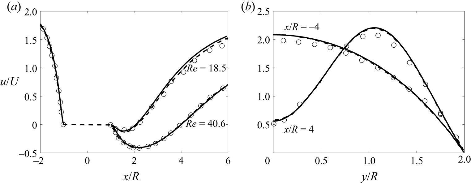
Streamwise velocity variation in the (a) streamwise direction at  $z/R=0$ and $y/R=0$ for $Re=18.5$ and $Re=40.6$ and (b) cross-stream direction at $z/R=0$ and $x/R=\pm 4$ for $Re=26.1$. Shown are the current simulations (black lines) and the numerical simulations (dashed black lines) and experiments (circles) by Ribeiro et al. (Reference Ribeiro, Coelho, Pinho and Alves2012).
The comparison with the analytical work by Thompson (Reference Thompson1968) forms the second part of the validation, which is for unbounded flow past a circular cylinder in a Hele-Shaw configuration. Extensive comparisons between the current numerical work and Thompson's analytical solution for a wide range of  $\varLambda$ are given in § 4, and are not repeated here. Also, as the comparison to Thompson's (Reference Thompson1968) paper forms a significant part of this work, the inner and outer solutions for the radial and tangential velocity and pressure have been included in Appendix B. Thompson's outer solution (for velocity and pressure) is given up to $\varLambda = {O}(\epsilon ^2)$, while the inner solution is up to $\varLambda = {O}(\epsilon )$, which needs to be considered when comparisons are made with the present direct numerical simulations.
3.2. Reduced system calculations
The reduced system descriptions are those of §§ 2.1–2.3. For the linear theory case of § 2.1, the outer flow is given by (2.11) and the inner flow by (2.12) and (2.13). These were treated by a standard relaxation method based on finite differences to determine the three scaled velocity components, which has been used in previous studies (Glowinski & Pironneau Reference Glowinski and Pironneau1979; Smith & Dennis Reference Smith and Dennis1990). The formulation here is a velocity–vorticity one, supplemented by iterative determination of the constant  $b$ through an integral of the continuity equation over the inner-region domain. Agreement was found with the results of Thompson (Reference Thompson1968) including the value 0.6302 of the constant $b$. The same finite-difference method was then extended to cover nonlinear range I for the system (2.17)–(2.18).
The system of equations in nonlinear range II (2.23) can be independently calculated in the  $z^*$– $r^*$ plane for different azimuthal locations. The question arises as to the length of the domain in the radial direction, as the boundary condition (2.24) is independent of $r^*$. One possibility is matching the asymptotic boundary condition for $u_r$ to the numerical simulation data, which is further explored in § 4.5.
4. Results: variation of  $\varLambda$

In this section, the results of the numerical simulations will be presented, and where appropriate compared to previous analytical work, for  $\epsilon =0.01$ and increasing $\varLambda$. These values have been chosen to highlight the different ranges identified in § 2. First, the velocity fields of the linear range will be presented, which also serves as further validation of the numerical methods. Next, as the nonlinear ranges identified in § 2 do not have explicitly defined limits, distinct flow phenomena cannot be allocated neatly to separate ranges. Therefore, flow and force diagnostics will be presented for increasing $\varLambda$, and the overall discussion is left to § 6.
4.1. Linear range
To investigate the linear range, simulations of  $\varLambda =0.001$ were carried out, such that $\varLambda \ll \epsilon \ll 1$. Figure 4 shows the comparison of the three velocity components between the current direct numerical simulations, reduced calculations and Thompson's analytical work at different azimuthal locations (which is measured from the rear stagnation point). In the outer region there is excellent agreement for the tangential, radial and vertical velocities between the current numerical simulations, Thompson's outer solution and the linear theory. In the inner region there is excellent agreement between the direct numerical simulations, reduced calculations and Thompson's inner solution. Note how the inner and outer solutions provide an agreeable composite solution to the numerical simulation results. The constant displacement thickness of approximately $0.6\epsilon$ can be identified as the vertical shift between the linear solution given by (2.9a–c) and the present simulations or Thompson's outer solution (see figure 4d); our calculation of $b$ in the linear range in § 2.1 is based on a solvability requirement that is equivalent to Thompson's approach and involves the total mass flux, and the result for $b$ agrees well with the numerical simulation results. The boundary layer thickness is approximately $r^*=2$, which was predicted in the early work by Stokes. The vertical velocity is orders of magnitude less than the radial and tangential velocities and is only present in the inner layer. The velocity profiles exhibit a symmetry around $\theta ={\rm \pi} /2$ for $\varLambda =0.001$, however as $\varLambda$ is increased the vertical and radial velocity become increasingly asymmetric.
The (a–c) tangential, (d–f) radial and (g–i) vertical velocity profiles at  $({a}, {d},{g})$ $\theta =3{\rm \pi} /4$, (b,e,h) $\theta ={\rm \pi} /2$ and (c,f,i) $\theta ={\rm \pi} /4$ for $\epsilon =0.01$ and $\varLambda =0.001$. The lines represent the present Navier–Stokes numerical simulations (black lines), present reduced calculations for the inner region (2.12)–(2.13) (green lines), Thompson's inner solution (blue lines and circles), Thompson's outer solution (red line) and the linear outer solution (2.11) (grey line). The profiles are in the midplane ( $z=0$) for (a–f) and at $z^*=-0.4$ for (g–i).

4.2. Streamlines perpendicular to cylinder surface
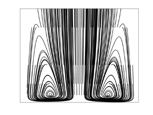
To gain a qualitative picture of the secondary flow induced by increasing  $\varLambda$, streamline plots of $u_z$ and $u_r$ (obtained from the direct numerical simulations) in planes perpendicular to the cylinder surface ( $z^*$– $r^*$), at different angles from the rear stagnation point, are shown in figure 5. In nonlinear range I, the important addition to the governing equations is the centrifugal term in (2.16), which occurs when $\varLambda$ is ${O}(\epsilon )$. For $\varLambda =0.05$, there is an upwelling in the component $u_r$ in the midplane (at $z^*=0$) at $\theta \approx {\rm \pi}/2$ (see figure 5b,c), which is a consequence of the centrifugal term (i.e. inertia) and occurs at the midplane because the centrifugal force is greatest there. For increasing $\varLambda$, the start of the upwelling moves closer to the front stagnation point, which is then followed by the streamlines wrapping around themselves, forming two counter-rotating vortices. Also, for the same angle from the rear stagnation point, these counter-rotating vortices increase in size for increasing $\varLambda$ (e.g. figure 5c,h,m for 92 $^{\circ }$). In figure 5, attention needs to be taken when considering the scale of the counter-rotating vortices. For example, for $\varLambda =1$, the two counter-rotating vortices grow to about $r^*=60$ (or $0.6R$) and as $\epsilon =0.01$, these are highly elongated flow structures (figure 5m).
Streamlines of  $u_z$ and $u_r$ in planes normal to the cylinder surface ( $z^*$– $r^*$) for (a–e) $\varLambda =0.05$, (f–j) $\varLambda =0.5$ and (k–o) $\varLambda =1$. All results are for $\epsilon =0.01$. The angle of the plane (from the rear stagnation point) is shown in the left corner. The red and green lines indicate the locations of where $u_r=0$ for Thompson's outer solution and the reduced calculations for nonlinear range I (2.13) and (2.16), respectively. Note the scale for $r^*$; for $\varLambda =1$, these are highly elongated vortices close to $\theta ={\rm \pi} /2$.

To compare the streamline structure of the direct numerical simulations against Thompson's (Reference Thompson1968) outer solution (red lines) and the current reduced calculations for nonlinear range I (2.16)–(2.18) (green lines), the locations of where  $u_r=0$ are shown in figure 5. Note that, in figure 5, for Thompson's work $u_r<0$ (i.e. the flow is towards the cylinder) and $u_r>0$ (i.e. the flow is away from the cylinder) for radial locations further away and closer to the cylinder than the red line, respectively. Thompson's work consistently underpredicts the results of the numerical simulations, while the comparison with the reduced calculations is good for azimuthal locations away from ${\rm \pi} /2$ and for low $\varLambda$. Metrics of the counter-rotating vortices are analysed in more detail in the next section. When $\theta <{\rm \pi} /2$, the pressure gradient and the centrifugal terms are coincident and the domed structure of where $u_r=0$ seen for $\theta >{\rm \pi} /2$ is not present. The counter-rotating vortices becoming smaller (for decreasing azimuthal location) and the flow towards the cylinder is increasingly confined to the channel walls (for $\theta$ tending towards zero).
4.3. Pair of counter-rotating vortices
The two metrics of interest here are the angle  $\theta _v$ at which the pair of counter-rotating vortices start to form (where the angle is measured from the rear stagnation point) and the size $L_v$ of the two counter-rotating vortices. Firstly, $\theta _v$ is defined to be the largest angle from the rear stagnation point, where $u_r=0$ along the radial coordinate, but that it is at least $r^*=2$ (see figure 6a). This definition is used to overcome the issue of Thompson's outer solution for $u_r$ not satisfying the no-slip condition on the cylinder surface (see the red line in figure 4d), so the outer solution for $u_r$ would predict the presence of streamwise vorticity, even in the linear regime. Figure 6(b) shows that, as $\varLambda$ is increased, the upwelling due to $u_r$ moves closer to the front stagnation point. The excellent agreement with the reduced calculations in figure 6(b) implies that the centrifugal term alone determines the starting point of the upwelling of $u_r$ for this range of $\varLambda$. Secondly, the size of the counter-rotating vortices is defined to be the distance from the cylinder surface in the midplane ( $z=0$) to where $u_r=0$ (see inset in figure 7a). For the reduced calculations, $L_v$ was found to be proportional to $\varLambda$. From the direct numerical simulations in figure 7(a,b), it can be seen that the growth of the counter-rotating vortices is not proportional to $\varLambda$ due to the additional nonlinear terms in (2.14) being important when $\varLambda$ is ${O}(1)$ and then only near $\theta ={\rm \pi} /2$.
(a) Definition of the angle  $\theta _v$ (where the flow is from left to right) and (b) its variation with $\varLambda$ (for $\epsilon =0.01$), where the present simulations are shown (circles), along with Thompson's theoretical value (red line) and the reduced calculations for nonlinear range I (green line).

Variation of the size of the counter-rotating vortices,  $L_v/R$, in the midplane at (a) $92^{\circ }$ and (b) 98 $^{\circ }$ with $\varLambda$ (for $\epsilon =0.01$), where the present simulations are shown (circles), along with Thompson's theoretical value (red line) and the reduced calculations for nonlinear range I (green line).

Thompson's (Reference Thompson1968) results in figures 6 and 7 are applicable up to  $\varLambda ={O}({1}$), while Thompson's inner solution (up to ${O}(\epsilon )$) for $u_r$ is symmetric about $\theta /{\rm \pi} =1/2$ and has no change of sign in the radial direction $r^*$ (and therefore cannot be used to predict $\theta _v$). In contrast, the reduced calculations in the current work are an inner solution. This might explain why Thompson's analysis is better at predicting $L_v$, while the present reduced calculations are better at predicting $\theta _v$. Although our interest here is to a large extent in the flow structure as $\varLambda$ increases, we should comment that in figure 7 the nonlinear range I results (in green) are almost certainly taken beyond their practical range of application.
4.4. Pressure field
In figure 8(a–c) the midplane surface pressure coefficient,  $(\tilde {p}_s-\tilde {p}_S)\varLambda /\rho U_c^2$, where $\tilde {p}_s$ and $\tilde {p}_S$ are the surface pressure and the pressure at the front stagnation point, respectively, is plotted for increasing $\varLambda$. For small $\varLambda$, the linear solution (2.9a–c) and Thompson's pressure solution (B4) agree with the current direct numerical simulations. For $\varLambda =1$, the agreement of the current simulations and Thompson's solution remains close while deviating from the Stokes solution. For $\varLambda =3$, Thompson's solution agrees with the simulations on the front side of the cylinder; however, it does not predict the behaviour on the rear side of the cylinder, significantly underestimating the drop in pressure there. Also plotted is the pressure perturbation of the direct numerical simulations from the linear solution (blue line), which is found to scale in proportion to $\varLambda \sin ^2\theta$ and is consistent with the asymptotic analysis and Thompson's analysis (see boundary condition (2.19) and Thompson's solution (B4), respectively).
The variation of the midplane ( $z=0$) surface pressure coefficient $(\tilde {p}_s-\tilde {p}_S)\varLambda /\rho U_c^2$ (where $\tilde {p}_S$ is the pressure at $\theta ={\rm \pi}$) with azimuthal location for the current direct numerical simulations (black line), the linear solution (black dashed lines) and Thompson's (Reference Thompson1968) solution (red lines) for $\varLambda =0.1$ (a), 1 (b) and 3 (c). The blue line gives the pressure perturbation of the direct numerical simulations from the linear solution.

In nonlinear range I, it is possible to calculate the gradients of the pressure perturbations (from the linear pressure solution) in the radial and the vertical directions. These pressure gradients, for example at the walls, were obtained from numerical derivatives of the vorticity functions that were used in the nonlinear range I calculations (see (C4) and (C5) in Appendix C). In figure 9(a) the inner solution of the present reduced calculations and Thompson's outer solution provide, in effect, an agreeable composite solution to the direct numerical simulations for the radial gradient of the pressure perturbation for  $\varLambda =0.1$. As $\varLambda$ is increased, the direct numerical simulations and the inner solution start to diverge, which is to be anticipated, as $\varLambda =1$ is beyond the range of applicability of nonlinear range I. Similarly, the numerical simulations start to diverge from Thompson's outer solution when $\varLambda$ is further increased to $\varLambda =3$. The vertical gradient of the surface pressure perturbation is plotted in figure 10(a). As could be anticipated, the variation is weak, and as $\varLambda$ is increased, the agreement between the nonlinear range I and the direct numerical simulations decreases. Note that Thompson does not calculate an inner pressure solution, so it is not possible to make comparisons with the current numerical simulations in this region.
Profiles of the radial gradient of the pressure perturbation for  $\varLambda =0.1$ (a), 1 (b) and 3 (c) for the current direct simulations (black lines), Thompson's outer solution (red lines) and nonlinear range I (green lines).

Profiles of the gradient of the (a) surface pressure perturbation in the vertical direction and (b) surface pressure minus the free-stream pressure  $\tilde {p}_{fs}$ in the azimuthal direction for the current direct simulations for $\varLambda =0.1$ ( $\square$), 1 ( $\bigcirc$) and 3 ( $\times$). Thompson's outer solution (red lines) and nonlinear range I (green lines) are also shown. The free-stream pressure, $\tilde {p}_{fs}(x)$, is the pressure in the channel far away from the cylinder (at the same streamwise location) projected onto the cylinder.

As the fluid flows through the channel and past the cylinder, there are two main pressure gradients, namely, the pressure gradient in the channel from the inlet to the outlet and also the pressure gradient due to the presence of the cylinder. When  $\varLambda$ is sufficiently small, the channel pressure gradient is dominant. However, as $\varLambda$ is increased, the channel pressure gradient is decreased, resulting in the cylinder pressure gradient having an increased effect on the flow. To highlight this, in figure 10(b), the free-stream pressure $p_{fs}(x)$ (i.e. far enough away for the cylinder to have no effect) is subtracted from the pressure at the surface of the cylinder. As expected, on the front of the cylinder there is a favourable pressure gradient (with reasonable agreement with Thompson's outer solution), but as $\varLambda$ is further increased, an adverse pressure gradient emerges at the rear of the cylinder at $\theta /{\rm \pi} \approx 0.4$ for $\varLambda =3$, which results in a deceleration in the tangential velocity at the back of the cylinder (see later figure 14f).
4.5. Velocity field
In this section the velocity field will be discussed for increasing  $\varLambda$. As the tangential velocity $u_{\theta }$ remains largely unchanged until $\varLambda$ is ${O}(1)$, we start with a detailed examination of $u_r$, which is instrumental in the formation of the counter-rotating vortices and is key to the reduced calculations in nonlinear range II, and then we progress to the tangential velocity. As $u_z$ is weak for the range of $\varLambda$ considered, it will not be discussed here.
To highlight how the secondary flow structure relates to the radial velocity, midplane velocity profiles of  $u_r$ are plotted in figure 11 for different $\varLambda$ at $\theta =3{\rm \pi} /4$. There is good agreement between the direct numerical simulations and the reduced calculations of this work for nonlinear range I (2.16)–(2.18) (see Appendix C for further details on how $u_r$ is calculated in nonlinear range I) and Thompson's outer and inner solutions where they are applicable, while for $\varLambda =3$, as is to be anticipated, there are significant differences. Note that $u_r=0$ was used to indicate the domed structure seen in figure 5.
The radial velocity profiles at  $\theta =3{\rm \pi} /4$ (in the midplane, $z=0$) for $\varLambda =0.1$ (a), 1 (b) and 3 (c). The lines represent the current Navier–Stokes numerical simulations (black line), Thompson's inner solution (blue circles), Thompson's outer solution (red line), the potential flow solution (grey line) and the reduced calculations for nonlinear range I (green line).

As  $\varLambda$ is increased from the linear to nonlinear range II, the boundary condition for the inner region at large $r^*$ changes. For the linear range, this boundary condition for $u_r$ at the cylinder is $(1-z^{*2})(1-r^{-2})\cos \theta$. When the centrifugal term is included and $\varLambda$ is increased, there are two components to the boundary condition (2.19). The first term is $2(r^*-b)(1-z^{*2})\cos \theta$, which is to be expected, based on the linear solution, and the second term is $\varLambda '\hat {u}_1$ (where $\varLambda '=\varLambda \epsilon ^{-1}$), which has three turning points and increases linearly with $\varLambda '$ (see end of § 2.2 for further discussion on this boundary condition). As the first term is dependent on $\cos \theta$ and the weighting of the second term is by $\varLambda '$, it is possible these terms are of equal magnitude, with a resulting velocity profile a combination of these two terms at different azimuthal locations for the same $\varLambda '$. For increasing $\varLambda '$, the three-turning-point velocity profile starts to emerge first at $\theta ={\rm \pi} /2$ due to the $\sin ^2\theta$ term in $\hat {u}_1$. This is the upwelling (due to the centrifugal term), which has already been discussed in the context of the generation of the counter-rotating vortices in § 4.2. When $\varLambda$ is still further increased into nonlinear range II, the boundary condition for $u_r$ at large $r^*$ only has one term, namely $\varLambda ''\hat {u}_1$.
To show the effect of varying azimuthal location and  $\varLambda$, profile plots of $u_r$ (in the vertical direction) at different radial locations from the cylinder surface are shown in figure 12, where the first row (a–c) and second row (d–f) are for $\theta =135^{\circ }$ and $\theta =95^{\circ }$, respectively; the latter is chosen to highlight the increased effect of inertia close to $\theta ={\rm \pi} /2$. The radial locations $r^*=50$ and $r^*=10$ are chosen to show how the velocity profile develops from large to small $r^*$ (note that for $\epsilon =0.01$, $r^*=50$ is equivalent to $0.5R$). A third velocity profile is also shown (with a dashed line), where the $u_r$ velocity profile is taken at the radial distance that best matches the asymptotic boundary condition (2.24). This always occurred at $r^*$ where the maximum positive $u_r$ value was attained (see figure 6a).
The radial velocity profiles (in the vertical direction) for (a–c)  $\theta =135^{\circ }$ and (d–f) $\theta =95^{\circ }$ for $\varLambda =0.05$ (a,d), 0.5 (b,e) and 1 (c,f). The three velocity profiles are at $r^*=50$ (solid line), $r^*=10$ (dots) and also the velocity profile where the numerical simulation results best match the asymptotic boundary condition (2.24) (green dashed lines). The colours represent the current numerical simulations (black) and Thompson's outer solution (red).

Figure 12(a–c) shows that, for  $\theta =135^{\circ }$ and an increase in $\varLambda$, the velocity profile remains almost unchanged for $r^*=50$, with a mild distortion arising in the profiles at $z^*=0$ (away from a parabolic shape) at $r^*=10$ and only resulting in the three-turning-point profile at $\varLambda =1$. For $\theta =95^{\circ }$ and $\varLambda =0.05$, the profiles for $r^*=1$ and $r^*=10$ are already distorted, however; even the closest matching velocity profile is quite different from the asymptotic boundary condition. It is quite likely that, for the flow conditions at this location, the two terms mentioned above are of approximately equal magnitude.
The reason for this in-depth look at  $u_r$ and its connection to the asymptotic boundary condition is because the nonlinear range II system of (2.23) does not have a defined domain length/size in $r^*$ (see boundary conditions (2.24)). One possibility is to set the domain length, $r^*_D$, to that where the current numerical simulation data best match the asymptotic boundary condition (2.24), the length of which was found to increase as $\varLambda$ increased (see figure 12d–f). Streamline plots of $u_z$ and $u_r$ at $98^{\circ }$ are shown in figure 13(a–c) for the direct numerical simulations. The radial locations of $r^*_D$ are highlighted by the blue dashed line (note that these are the dashed line velocity profiles in figure 12d–f). In figure 13(d–f) are shown the streamlines for nonlinear range II. There are considerable differences between the simulation results and the nonlinear range II streamlines, which is likely to be due to the zero vertical velocity imposed at the ‘inlet’ of nonlinear II calculations, which is not the case for the direct numerical simulations. For these confined flows, the flow field will be very sensitive to these imposed boundary conditions.
Streamlines of  $u_z$ and $u_r$ in planes normal to the cylinder surface ( $z^*$– $r^*$) at $98^{\circ }$ for $\varLambda =0.05$ (a,d), 0.5 (b,e) and 1 (c,f) for the direct numerical simulations (a–c) and nonlinear range II (2.23) (d–f). In (a–c) the blue dashed line indicates $r_D^*$, where the asymptotic boundary condition (2.24) best matches the current simulation results.

As  $\varLambda$ is increased, the pair of counter-rotating vortices form closer to the front stagnation point and also become larger, which results in the momentum in the radial and vertical directions increasing and hence the momentum in the azimuthal direction decreasing. The consequence is a negative displacement thickness at the front of the cylinder, which can be seen in figure 14(a–c), where the tangential velocity at $\theta =3{\rm \pi} /4$ is less than that of the potential flow as $\varLambda$ is increased from 0.1 to 3. An increase in $\varLambda$ also results in the adverse pressure gradient emerging at the back of the cylinder, which results in a deceleration of the tangential velocity, an effect that is quite pronounced for $\varLambda =10$ (see figure 14f).
The tangential velocity profiles for (a–c)  $\theta =3{\rm \pi} /4$ and (d–f) $\theta ={\rm \pi} /4$ for $\varLambda =0.1$ (a,d), 1 (b,d) and 3 (c,f). All profiles are in the midplane, $z=0$. The lines represent the current Navier–Stokes numerical simulations (black line), Thompson's inner solution (blue line), Thompson's outer solution (red line) and the potential flow solution (grey line).

4.6. Limit of steady flow with increasing $\varLambda$

For  $\varLambda \gg 1$, the channel Reynolds number $Re_h=U_ch/\nu$ becomes a potentially limiting factor to a steady flow and is especially important for flows past circular cylinders, as the fluid has to accelerate around the sides. The critical Reynolds number for flow in a channel is approximately 800 (Tuckerman et al. Reference Tuckerman, Kreilos, Schrobsdorff, Schneider and Gibson2014), which for $\epsilon =0.01$ is $\varLambda =8$. The highest value for $\varLambda$ that was simulated with the steady-state solver was $\varLambda =3$ and a simulation of $\varLambda =5$ did not converge. No further attempt was made to obtain an exact point of transition with a transient solver or to investigate the instability mechanism. How this upper limit on $Re_h$ affects the flow past a circular cylinder is discussed further in § 6.
4.7. Drag force
The force on the cylinder is
 \begin{equation} {\boldsymbol F} = \int_S (\tilde{p}{\boldsymbol{{\mathsf{I}}}}-{\boldsymbol \tau}) \boldsymbol{\cdot}{\hat{\boldsymbol{n}}}\,{\rm d}S, \end{equation}
where  ${\boldsymbol { {\mathsf {I}}}}$ and ${\boldsymbol \tau }$ are the identity matrix and viscous stress tensor, respectively, and $\hat {\boldsymbol {n}}$ is the unit vector out of the fluid domain. The corresponding drag coefficient is defined as
 \begin{equation} C_D = \frac{{\boldsymbol F}\boldsymbol{\cdot}{\hat{\boldsymbol{x}}}}{2\rho U_c^2hR}, \end{equation}
which can be split into the pressure and the viscous components,
 \begin{equation} C_{DP}= \frac{\int_S\tilde{p}{\boldsymbol{{\mathsf{I}}}}\hat{\boldsymbol{n}} \boldsymbol{\cdot}{\hat{\boldsymbol{x}}}\,{\rm d}S}{2\rho U_c^2hR},\quad C_{D\nu}=C_D-C_{DP}, \end{equation}
where  $\hat {\boldsymbol {x}}$ is the unit vector in the streamwise direction (Klettner et al. Reference Klettner, Eames, Semsarzadeh and Nicolle2016). The drag coefficient is plotted in figure 15(b) with the numerical simulations compared with Lee & Fung's (Reference Lee and Fung1969) Stokes solution and also a direct calculation with (4.1) using Thompson's analysis. The two methods give the same prediction, although Thompson's analysis gives a better agreement for the surface pressure for $\varLambda =3$ (figure 8c), which is due to the form of the $\varLambda$ term in (B4).
(a) Drag coefficient as a function of  $\varLambda$; the current numerical simulations are shown as circles, Lee & Fung's (Reference Lee and Fung1969) force expression for a Stokes flow past a cylinder is shown as a black dashed line and Thompson's analytical solution is given by the red lines. All results are for $\epsilon =0.01$. (b) The midplane friction coefficient for $\varLambda =0.1$ ( $\square$), 1 ( $\bigcirc$) and 3 ( $\times$).

An alternative way of calculating the drag force would be using an integral analysis, where, due to diffusion, velocity perturbations in the wake disappear quickly behind the cylinder (Lee & Fung Reference Lee and Fung1969). The friction coefficient  $\tilde {\tau }_w\varLambda /(\rho U_c^2)$ with $\tilde {\tau }_w=\mu \, \partial \tilde {u}_{\theta }/\partial \tilde {r}$ on the cylinder midplane is plotted for the direct numerical simulations and Thompson's (Reference Thompson1968) inner solution in figure 15(b) for increasing $\varLambda$. The boundary layer thickness around the front of the cylinder decreases slightly for increasing $\varLambda$, leading to an increase in the shear stress for $-1<\theta /{\rm \pi} <-1/2$ (figure 15b), which is not predicted by Thompson's inner solution, as it has no dependence on $\varLambda$ (see (B3)). Agreement is good up to where the inner solution is applicable; however, the deceleration of the tangential velocity is not captured at the rear of the cylinder. The friction coefficient is two orders of magnitude less than the pressure and also decreases significantly towards the sidewalls, which results in $C_{DP}/C_D \approx 1$.
5. Results: variation of $\epsilon$

In this section the variation of  $\epsilon$ is investigated with $\epsilon =0.1$ and varying $\varLambda$. The main difference in increasing $\varLambda$ at $\epsilon =0.1$ is that the channel instability occurs now at $\varLambda =80$, which means that the flow features already analysed in § 4 can develop further, and also results in additional flow phenomena. Also, simulations are carried out to explore the parameter space $\varLambda$– $\epsilon$, and these results are discussed in the next section.
The metric  $\theta _v$ was found to be quite different for $\epsilon =0.1$ than for $\epsilon =0.01$. Figure 16(a) shows that the angle at which the secondary flow starts to form is closer to $\theta /{\rm \pi} =1/2$ and also that $\theta _v$ is quite insensitive to $\varLambda$ for $\varLambda \gg 1$. For $\epsilon =0.1$, the boundary layer is thicker than for $\epsilon =0.01$, which results in the tangential velocity having a smaller magnitude around the front of the cylinder (compare figure 14(d–f) with figure 17), which means that the centrifugal effect that causes the secondary flow is weakened, and as such the vortices form further away from the front stagnation point. Figure 16(b) shows the variation of the metric $L_v$ with $\varLambda$ (at $\theta =98^{\circ }$). For $\varLambda =1$ the counter-rotating vortices are quite similar in size to $\epsilon =0.01$ (both are $L_v/R \approx 0.2$; see figure 7b). For $\varLambda =10$, these grow to $L_v/R \approx 1$. The prediction from Thompson's analysis is also shown; however, it should be noted that this is taken well past where it is applicable. Additional simulations were also carried out to investigate the effect of increasing $\epsilon$ on the secondary flow. As $\epsilon$ was increased from 0.2 to 0.5, the secondary flow that is generated is smaller and confined closer to the sidewalls as compared to $\epsilon =0.01$ (see for example figure 5).
(a) Variation of the angle  $\theta _v$ with $\varLambda$. (b) Variation of the size of the counter-rotating vortices with $\varLambda$ in the midplane at 98 $^{\circ }$. Thompson's analytical solution is given by the red line. All results are for $\epsilon =0.1$.

The tangential velocity profiles for  $\epsilon =0.1$ and $\varLambda = 0.1$ (a), 1 (b) and 10 (c) at $\theta =3{\rm \pi} /4$. All profiles are in the midplane. The lines represent the current numerical simulations (black line), Thompson's inner solution (blue line), Thompson's outer solution (red line) and the potential flow solution (grey line). To highlight the deceleration at the back of the cylinder, the dashed line in panels (b) and (c) is the velocity profile at $\theta ={\rm \pi} /4$.

The tangential velocity profiles follow those seen previously for  $\epsilon$, with good agreement between the direct numerical simulations and Thompson's solution (see figure 17). The displacement thickness is clearly visible in figure 17(a), as the red line is $0.6\epsilon$ above the potential flow solution. Although there is no negative displacement thickness at $\varLambda =1$, the tangential velocity for $\varLambda =10$ is considerably less than the potential flow solution. The comparison is good at the front of the cylinder, even for $\varLambda =10$. To highlight the effect of the adverse pressure gradient at the back of the cylinder, a profile is also given at ${\rm \pi} /4$ with significant deceleration for $\varLambda =10$.
For  $\epsilon =0.1$, the midplane friction and the surface pressure coefficient are plotted in figure 18. Similar to $\epsilon =0.01$, there is good agreement for the surface pressure coefficient for $\varLambda =0.1$ and 1. For $\varLambda =10$ there is an adverse pressure gradient at $\theta /{\rm \pi} \approx \pm 0.4$. Owing to the deceleration in the tangential velocity at the rear of the cylinder, the friction coefficient is negligible here for $\varLambda =10$. Note the increase in the friction coefficient over the front side of the cylinder for $\varLambda =10$. In comparison to $\epsilon =0.01$, the friction coefficient is only an order of magnitude less than the pressure coefficient, which results in the pressure component of the drag coefficient being $C_{DP}/C_D\approx 0.95$. The dependence of $C_D$ on $\epsilon$ (see Lee & Fung Reference Lee and Fung1969) is present, but it is not possible to distinguish this from figures 15 and 18.
(a) The midplane friction coefficient for  $\varLambda =0.1$ ( $\square$), 1 ( $\bigcirc$) and 10 ( $\times$). (b) The pressure coefficient for $\varLambda =0.1$, 1 and 10. (c) Drag coefficient as a function of $\varLambda$; the current numerical simulations are shown as circles, Lee & Fung's (Reference Lee and Fung1969) force expression for a Stokes flow past a cylinder is shown as a black dashed line and Thompson's analytical solution is given by the red line. All results are for $\epsilon =0.1$.

The consequence of the adverse pressure gradient and the subsequent deceleration in the tangential velocity is a laminar separation bubble (LSB) forming at the rear of the cylinder for  $\varLambda _s \approx 13.5$ ( $\varLambda _s$ here is the minimum value of $\varLambda$ at which the LSB forms). Figure 19 shows streamlines of the velocity field in blue while the LSB is highlighted with red streamlines. The LSB is of size ${O}(h)$ as indicated by the black dashed line around the cylinder. When $\varLambda$ is further increased, the LSB forms into an attached separation bubble, which is seen in two-dimensional flow past cylinders up to a Reynolds number of about 40. Figure 20 shows that decreasing $\epsilon$ decreased the size of the LSB and also shifted its formation towards the front stagnation point. Also, as $\epsilon$ decreases, $\varLambda _s$ increases.
Streamlines of the velocity field (in blue) highlighting the development of the laminar separation bubble (red streamlines) in the midplane for  $\epsilon =0.1$ and $\varLambda =13.5$ (a) ( $\approx \varLambda _s$), 19 (b) and 25 (c). The black dashed line indicates the distance $\epsilon$ from the cylinder surface. The flow is from left to right.

Streamlines of the velocity field (in blue) highlighting the laminar separation bubble (red streamlines) in the midplane ( $z=0$) for $\epsilon = 0.1$ (a), 0.05 (b) and 0.031 (c) for $\varLambda \approx \varLambda _s$. The black dashed line indicates the half-height $h$. The flow is from left to right.

6. Discussion and conclusions
Our concern in the paper has been with the effects of increasing nonlinearity, represented by increasing values of the parameter  $\varLambda$, in a Hele-Shaw configuration with a circular cylinder in a channel. The study has consisted of direct numerical simulations for small finite ratios ( $\epsilon$) of channel half-height to cylinder radius supplemented by analyses for asymptotically small ratios.
It is insightful to summarise the work in the preceding sections into a plot of the parameter space  $\varLambda$– $\epsilon$ (see figure 21). Traditional Hele-Shaw flow is for $\varLambda \ll 1$ and $\epsilon \ll 1$. In § 2 the linear range and the nonlinear ranges I, II and III were identified, which correspond to $\varLambda$ being ${O}(\epsilon )$, ${O}(\epsilon ^{1/2})$ and ${O}(1)$, respectively. In § 4 the upper limit, as $\varLambda$ is increased, of the steady flow was suggested as due to unsteady Poiseuille flow (shown as a green dashed line). In § 5, as $\epsilon$ was increased to approximately $0.3<\epsilon <0.5$, the secondary flow was no longer present as two counter-rotating vortices; instead, smaller vortices formed adjacent to the sidewalls (represented by a red dashed line). Also there is the steady separated flow region for $\epsilon \gtrsim 0.03$ and increasing $\varLambda$. The region where Thompson's inner and outer analyses are applicable is for $\varLambda ={O}(\epsilon )$ and ${O}(1)$, respectively, and $\epsilon \ll 1$. In nonlinear range I, the secondary flow starts to emerge, and this is followed by a negative displacement thickness at the front of the cylinder in nonlinear range II and a deceleration of the tangential velocity around the back of the cylinder in nonlinear range III. The suggested form of nonlinear range III implies that the three-dimensional interactive boundary layer (IBL) equations hold throughout the outer region then. Three-dimensional IBL theory is usually used for external flows (Smith Reference Smith1983; Duck & Burggraf Reference Duck and Burggraf1986; Smith Reference Smith2018) rather than for the present internal configuration.
A diagram summarising the different ranges for the flow past a circular cylinder in a Hele-Shaw configuration with the linear and nonlinear (NL) ranges I, II and III analysed in § 2. The dashed red line indicates the approximate upper limit of the formation of the secondary flow (as two counter-rotating vortices as in figure 5) and the dashed green line indicates the approximate transition to an unsteady Poiseuille flow. The blue dashed line indicates steady separated flow. The simulations carried out are indicated by  $\bullet$.

Further investigation is required to establish how and when the unsteady flow might occur as  $\varLambda$ is increased. There are two different flow fields that can be present before the unsteadiness occurs, namely a steady separated flow (for $0.2 \gtrsim \epsilon \gtrsim 0.03$) and a non-separated flow ( $\epsilon \lesssim 0.03$), which are likely to respond differently to an increase in $\varLambda$. Additionally, as the flow has to accelerate around the cylinder, the flow might go unsteady earlier than indicated in the figure (i.e. the dashed green line in figure 21 could be shifted to the left). The three-dimensional nature of these separation bubbles is also left to further work.
In this work there was extensive comparison made between our reduced calculations in nonlinear range I, direct numerical simulations and Thompson's analysis. Thompson's use of matched asymptotics meant that there was some feedback between the inner and outer regions. There is interesting overlap of Thompson's and the present analytical work. Thompson's excellent work is mostly concerned with effects such as higher-order influences in the outer region. In contrast, we find analytically that nonlinearity first enters at leading order in the inner region as far as the secondary flow is concerned and, in a second stage, nonlinearity is much increased to the extent that the main flow velocity component becomes altered nonlinearly. Both of these inner-region stages occur with the parameter  $\varLambda$ still being small. The advantage of treating the fully nonlinear problem by direct simulation, allied with analysis, is felt to be that clear ranges can be identified when certain phenomena are likely to occur.
Acknowledgements
The authors acknowledge the use of University College London's Myriad High Performance Computing Facility (Myriad@UCL) and Kathleen High Performance Computing Facility (Kathleen@UCL), and associated support services, in the completion of this work.
Declaration of interests
The authors report no conflict of interest.
Author contributions
C.A.K. performed the OpenFoam numerical simulations. F.T.S. carried out the asymptotic analysis. Both authors contributed equally to analysing data, reaching conclusions and writing the paper.
Appendix A
This appendix will detail the mesh independence study. Boundary layers in Hele-Shaw flow are not like the more common inviscid–viscous boundary layers (where the boundary layer thickness can be estimated by equating viscous and inertial forces). Here the boundary layer thickness does not vary significantly with  $\varLambda$ and is dependent on the gap height $2h$. As this is a three-dimensional problem, mesh independence will be shown in the three cylindrical coordinates.
Firstly, for the radial and azimuthal directions, the case of  $\epsilon =0.01$ and $\varLambda =0.001$ is chosen. From figure 4, we can see that, although the boundary layer thickness is $r^*=2$, the gradient of the vertical velocity changes sign at $r^*\approx 0.5$, making $u_z$ the velocity component with the highest mesh resolution requirement. Figure 22 shows meshes of increasing radial resolution $\varDelta _r/R=\{0.0017, 0.0011, 0.0008\}$ or $\varDelta _r/h=\{0.17, 0.11, 0.08\}$, with the coarsest visibly not resolving the vertical velocity close to the wall while the finest mesh adequately resolves it.
Mesh independence study of the vertical velocity at  $\theta =3{\rm \pi} /4$ for $\epsilon =0.01$, $\varLambda =0.001$ and $z^*=0.4$ for $\varDelta _r/h= 0.17$ (a), 0.11 (b) and 0.08 (c). The vertical mesh resolution is shown to the left of the velocity profiles. Also shown are the current reduced simulations for nonlinear range I (green lines) and Thompson's inner solution (blue circles).

It should be noted that the mesh resolution required for the vertical velocity is considerably greater than the tangential velocity. To highlight this, the friction coefficient  $\tilde {\tau }_w\varLambda /(\rho U_c^2)$ on the cylinder midplane is plotted and compared to Thompson's analytical solution, with all resolutions showing excellent agreement (see figure 23). Additionally, the pressure coefficient is shown, which highlights that these surface metrics are not sensitive to the meshes used. Additional integral metrics (e.g. drag coefficient) have not been included in this mesh independence study, as the surface metrics indicate that an adequate resolution is present. This also indicates that the resolution requirement in the azimuthal direction is not as great in the radial direction, and so $\varDelta _{\theta } \approx 4 \varDelta _r$.
Mesh independence study of (a) the friction coefficient and (b) the pressure coefficient for  $\epsilon =0.01$, $\varLambda =0.001$ and $z^*=0$ with $\varDelta _r/h=0.17$ ( $\square$), 0.11 ( $\bigcirc$) and 0.08 ( $\times$). Also shown are Thompson's inner solution for the friction coefficient and the outer solution for the pressure (red lines).

For the vertical direction, the case chosen for mesh independence is  $\varLambda =1$ and $\epsilon =0.01$. The vertical profile of the radial velocity $u_r$ (i.e. in the $z^*$-direction) at $r^*=4$ was chosen (see figure 12f), as the velocity profile has three turning points, therefore requiring a higher resolution than the parabolic profiles usually encountered in Hele-Shaw type flows. Radial velocity profiles were compared for increasing mesh densities of $\varDelta _z/h=\{0.095,0.065,0.049\}$ (while keeping $\varDelta _r/h=0.08$) and all meshes provided adequate resolution (plots not shown here).
The final meshes used a mesh resolution close to the cylinder of  $\varDelta _r/h=0.08$, $\varDelta _{\theta }=0.32$ and $\varDelta _z=0.049$. In the vertical direction, the mesh spacing is equal whereas the mesh spacing in the radial direction is finer towards the cylinder surface. Note that away from the cylinder the mesh size increases, which results in quite elongated elements far from the cylinder. However, the Poiseuille flow that is present in this region is insensitive to these elements.
Appendix B
This appendix states Thompson's (Reference Thompson1968) tangential and radial velocities and pressure for the outer and inner flow regions. The outer solution for the tangential velocity is given by
 \begin{align} u_{\theta} &= \underbrace{ -(1-z^{*2})\left(1+\frac{1}{r^2}\right)\sin\theta }_{{O}(1)} - \underbrace{ \frac{1}{2}\epsilon(1-z^{*2})\frac{\phi_1\sin\theta}{r^2} }_{{O}(\epsilon)} \nonumber\\ &\quad \underbrace{-\frac{1}{18}\epsilon^2\phi_1^2(1-z^{*2})\frac{\sin\theta}{r^2} + \varLambda H(z^*)\frac{\sin 2\theta}{r^3}}_{{O}(\epsilon^2)}, \end{align}
where  $H(z^*)=z^{*6}/15-z^{*4}/3+11z^{*2}/35-1/21$ and $\phi _1=2.521$; and the radial velocity is given by
 \begin{align} u_r &= \underbrace{ (1-z^{*2})\left(1-\frac{1}{r^2}\right)\cos\theta }_{{O}(1)}- \underbrace{\frac{1}{2}\epsilon(1-z^{*2})\frac{\phi_1\cos\theta}{r^2} }_{{O}(\epsilon)} \nonumber\\ &\quad \underbrace{-\frac{1}{18}\epsilon^2\phi_1^2(1-z^{*2})\frac{\cos\theta}{r^2} + \varLambda H(z^*) \left(\frac{\cos 2\theta}{r^3} -\frac{1}{r^5} \right)}_{{O}(\epsilon^2)}. \end{align}
The inner solution for the tangential velocity, to  ${O}(\epsilon )$, is given by
 \begin{align} u_{\theta} &= \underbrace{-2\left(1-z^{*2}-4\sum_{n=0}^{\infty}(-)^nk_n^{{-}3}\,{\rm e}^{{-}k_nr^*} \cos k_nz^{*} \right)\sin\theta}_{{O}(1)} \nonumber\\ &\quad \underbrace{-\frac{1}{2}\epsilon\sin\theta \left\{\left((1-z^{*2})(\phi_1-4r^*)-\phi_1\sum_{n=0}^{\infty}(-)^nk_n^{{-}3}\,{\rm e}^{{-}k_nr^*}\cos k_nz^* \right)\right\}}_{{O}(\epsilon)}, \end{align}
where  $k_n=(n+1/2){\rm \pi}$. The inner solutions, to ${O}(\epsilon )$, for the radial and vertical velocities are tabulated in Thompson (Reference Thompson1968). The outer pressure, to ${O}(\epsilon ^2)$, in Thompson (Reference Thompson1968) is given by
 \begin{equation} p={-}2\cos\theta\left( r+\frac{1+\tfrac{1}{2}\epsilon\phi_1+ \tfrac{1}{18}\epsilon^2\phi_1^2}{r} \right) - \frac{12}{35}\varLambda\left(1-\frac{2\cos 2\theta}{r^2} + \frac{1}{r^4} \right),\end{equation}
noting the typographical error in Thompson's (Reference Thompson1968) equation (4.12).
Appendix C
In this appendix the solution to nonlinear range I, (2.13) and (2.16), is described. The radial velocity  $u_r$ close to the cylinder is given by
 \begin{equation} u_r = 2 V_1(r^*, z^*) \epsilon \cos\theta + 4 V_2(r^*, z^*) \varLambda \sin^2\theta, \end{equation}
while further out the above expression reduces to
 \begin{equation} u_r = 2 V_{1\infty}(r^*, z^*) \epsilon \cos\theta + 4 V_{2\infty}(z^*) \varLambda \sin^2\theta, \end{equation}
with
 \begin{equation} V_{1\infty}(r^*, z^*) = (r^* -b) (1 -z^{*2}), \quad V_{2\infty}(z^*) = \tfrac{1}{42} -\tfrac{11}{70} z^{*2} + \tfrac{1}{6}z^{*4} - \tfrac{1}{30}z^{*6}, \end{equation}
where  $b=0.63$. The functions $V_1$, $V_2$ and $V_{1\infty }$ are plotted in figure 24(a,b). The gradient of the pressure perturbation in the radial and vertical directions in nonlinear range I are given by
 \begin{equation} \frac{\partial \hat{p}}{\partial r^*}= 2\frac{\partial P_{r1}}{\partial r^*}\cos\theta + \frac{\partial P_{r2}}{\partial r^*}\left(\frac{4\varLambda}{\epsilon}\right)\sin^2\theta \end{equation}
and
 \begin{equation} \frac{\partial \hat{p}}{\partial z^*}= 2\frac{\partial P_{z1}}{\partial z^*}\cos\theta + \frac{\partial P_{z2}}{\partial z^*}\left(\frac{4\varLambda}{\epsilon}\right)\sin^2\theta, \end{equation}
respectively, where the additional functions on the right-hand sides are plotted in figure 24(c,d).
The variation of the functions (a)  $V_1$, (b) $V_2$ and (c) $\partial P_{r1}/\partial r^*$ and $\partial P_{r2}/\partial r^*$ with radial distance, and (d) $\partial P_{z1}/\partial z^*$ and $\partial P_{z2}/\partial z^*$ with vertical position. Panels (a) and (b) show different values of $z^*$ from $-$0.9 to 0, (c) are the midplane values and (d) are for the cylinder surface. The dashed lines in (a) are the functions $V_{1\infty }$.


 Open access