





1. Introduction
The attached eddy hypothesis (AEH) of A. A. Townsend (Reference Townsend1976), along with several decades of subsequent investigations (Marusic & Monty Reference Marusic and Monty2019), is a key advancement in describing turbulent statistics in canonical wall-bounded flows. The AEH provides a phenomenological link between the turbulence, the logarithmic mean velocity profile and the logarithmic decay in the streamwise and spanwise velocity variances. These trends have all been supported by measurements at sufficiently high Reynolds numbers across various canonical wall-bounded flows (see, e.g. Jiménez & Hoyas Reference Jiménez and Hoyas2008; Hultmark et al. Reference Hultmark, Vallikivi, Bailey and Smits2012; Marusic et al. Reference Marusic, Monty, Hultmark and Smits2013; Orlandi, Bernardini & Pirozzoli Reference Orlandi, Bernardini and Pirozzoli2015; Lee & Moser Reference Lee and Moser2015) including the near-neutral atmospheric surface layer (Puccioni et al. Reference Puccioni, Calaf, Pardyjak, Hoch, Morrison, Perelet and Iungo2023; Qin et al. Reference Qin, Katul, Liu and Li2025).
The population of attached eddies envisioned by Townsend also produces a constant wall-normal velocity variance $\overline {w^{\prime 2}}$
within the logarithmic region of the boundary layer
$\overline {w^{\prime 2}}$
within the logarithmic region of the boundary layer
 \begin{align} \dfrac {\overline {w^{\prime 2}}(z)}{ U_{\tau }^2} = B_3, \end{align}
which is proportional to the surface shear (friction) velocity $U_\tau = \sqrt {\tau _w/\rho }$
corresponding to the wall shear stress
$U_\tau = \sqrt {\tau _w/\rho }$
corresponding to the wall shear stress $\tau _w$
and fluid density
$\tau _w$
and fluid density $\rho$
. Wall-normal profiles of
$\rho$
. Wall-normal profiles of $\overline {w^{\prime 2}}$
tend to vary only weakly within the logarithmic region (Morrill-Winter et al. Reference Morrill-Winter, Klewicki, Baidya and Marusic2015; Qin et al. Reference Qin, Katul, Liu and Li2025) and there is evidence for a constant third-order skewness (Buono et al. Reference Buono, Katul, Heisel, Vettori, Poggi, Peruzzi and Manes2024b
). Yet, there is no conclusive universal value for
$\overline {w^{\prime 2}}$
tend to vary only weakly within the logarithmic region (Morrill-Winter et al. Reference Morrill-Winter, Klewicki, Baidya and Marusic2015; Qin et al. Reference Qin, Katul, Liu and Li2025) and there is evidence for a constant third-order skewness (Buono et al. Reference Buono, Katul, Heisel, Vettori, Poggi, Peruzzi and Manes2024b
). Yet, there is no conclusive universal value for $B_3$
from observations and (1.1) has the least experimental support among the statistics predicted by the AEH (Buono et al. Reference Buono, Katul, Heisel, Poggi, Peruzzi, Vettori and Manes2024a
).
$B_3$
from observations and (1.1) has the least experimental support among the statistics predicted by the AEH (Buono et al. Reference Buono, Katul, Heisel, Poggi, Peruzzi, Vettori and Manes2024a
).
There are two primary challenges in determining the value of $B_3$
. The first is that the AEH models an asymptotically high-Reynolds-number wall-bounded flow with negligible viscosity effects within the logarithmic region. Observations of
$B_3$
. The first is that the AEH models an asymptotically high-Reynolds-number wall-bounded flow with negligible viscosity effects within the logarithmic region. Observations of $\overline {w^{\prime 2}}$
in available simulations and laboratory-scale experiments are limited to finite Reynolds number and must account for its dependence. An example is shown in figure 1(a) for direct numerical simulations (DNSs) of flows in a zero-pressure-gradient (ZPG) flat plate turbulent boundary layer (TBL) (Sillero, Jiménez & Moser Reference Sillero, Jiménez and Moser2013), channel (Lee & Moser Reference Lee and Moser2015) and pipe (Yao et al. Reference Yao, Rezaeiravesh, Schlatter and Hussain2023). The
$\overline {w^{\prime 2}}$
in available simulations and laboratory-scale experiments are limited to finite Reynolds number and must account for its dependence. An example is shown in figure 1(a) for direct numerical simulations (DNSs) of flows in a zero-pressure-gradient (ZPG) flat plate turbulent boundary layer (TBL) (Sillero, Jiménez & Moser Reference Sillero, Jiménez and Moser2013), channel (Lee & Moser Reference Lee and Moser2015) and pipe (Yao et al. Reference Yao, Rezaeiravesh, Schlatter and Hussain2023). The $\overline {w^{\prime 2}}$
value for channel and pipe flows is nearly constant across intermediate distances, but the magnitude increases with the friction Reynolds number
$\overline {w^{\prime 2}}$
value for channel and pipe flows is nearly constant across intermediate distances, but the magnitude increases with the friction Reynolds number $ \textit{Re}_\tau = U_\tau \delta / \nu$
, with
$ \textit{Re}_\tau = U_\tau \delta / \nu$
, with $\delta$
being the boundary layer thickness and
$\delta$
being the boundary layer thickness and $\nu$
the kinematic viscosity.
$\nu$
the kinematic viscosity.
Perry and co-authors (Reference Perry, Henbest and Chong1986, Reference Perry and Li1990) estimated this Reynolds-number dependence by considering the finite scale separation between the wall parameters and the viscous motions in the spectrum of $w$
, resulting in a correction for
$w$
, resulting in a correction for $B_3$
as a function of
$B_3$
as a function of $z^+ = z U_\tau / \nu$
. An alternative approach was recently proposed by Spalart & Abe (Reference Spalart and Abe2021), who used extrapolation of profiles at different Reynolds numbers following the technique of Luchini (Reference Luchini2017). The method accurately describes channel data (Hoyas, Oberlack & Laux Reference Hoyas, Oberlack, Alcántara-Á vila, Kraheberger and Laux2022), but is empirical in nature and is not linked to the flow phenomenology. These previous efforts collectively have not produced a conclusive Reynolds-number correction to (1.1) and further research on the matter is warranted.
$z^+ = z U_\tau / \nu$
. An alternative approach was recently proposed by Spalart & Abe (Reference Spalart and Abe2021), who used extrapolation of profiles at different Reynolds numbers following the technique of Luchini (Reference Luchini2017). The method accurately describes channel data (Hoyas, Oberlack & Laux Reference Hoyas, Oberlack, Alcántara-Á vila, Kraheberger and Laux2022), but is empirical in nature and is not linked to the flow phenomenology. These previous efforts collectively have not produced a conclusive Reynolds-number correction to (1.1) and further research on the matter is warranted.
Profiles of the wall-normal velocity variance $\overline {{w^\prime }^2}$
normalised by the surface shear velocity
$\overline {{w^\prime }^2}$
normalised by the surface shear velocity $U_{\tau }$
: (a) wall-normal position
$U_{\tau }$
: (a) wall-normal position $z$
in viscous units
$z$
in viscous units $z^+=z U_\tau / \nu$
; (b)
$z^+=z U_\tau / \nu$
; (b) $z$
in outer units relative to the boundary layer thickness
$z$
in outer units relative to the boundary layer thickness $\delta$
. In all figures, the data are from DNSs (Sillero et al. Reference Sillero, Jiménez and Moser2013; Lee & Moser Reference Lee and Moser2015; Yao et al. Reference Yao, Rezaeiravesh, Schlatter and Hussain2023), with colour indicating the flow case and shade corresponding to the friction Reynolds numbers
$\delta$
. In all figures, the data are from DNSs (Sillero et al. Reference Sillero, Jiménez and Moser2013; Lee & Moser Reference Lee and Moser2015; Yao et al. Reference Yao, Rezaeiravesh, Schlatter and Hussain2023), with colour indicating the flow case and shade corresponding to the friction Reynolds numbers $ \textit{Re}_\tau = \delta U_\tau /\nu$
given in table 1.
$ \textit{Re}_\tau = \delta U_\tau /\nu$
given in table 1.

The exclusion of viscous effects in the AEH applies also to the Reynolds shear stress $\overline {u^\prime w^\prime }$
. The assumption of a constant turbulent stress with negligible viscous stress contribution is an ansatz of the AEH
$\overline {u^\prime w^\prime }$
. The assumption of a constant turbulent stress with negligible viscous stress contribution is an ansatz of the AEH
 \begin{align} \dfrac {-\overline {u^\prime w^\prime }(z)}{ U_{\tau }^2} = 1. \end{align}
Equation (1.2) further neglects any decrease in the total stress profile below $U_\tau ^2$
as the wall-normal distance increases. Given that
$U_\tau ^2$
as the wall-normal distance increases. Given that $\overline {w^{\prime 2}}$
and
$\overline {w^{\prime 2}}$
and $\overline {u^\prime w^\prime }$
have both been postulated to receive contributions solely from the ‘active’ motions per Townsend’s (Reference Townsend1976) AEH, viscous stresses and a decreasing total stress can directly impact
$\overline {u^\prime w^\prime }$
have both been postulated to receive contributions solely from the ‘active’ motions per Townsend’s (Reference Townsend1976) AEH, viscous stresses and a decreasing total stress can directly impact $\overline {w^{\prime 2}}$
. This has been demonstrated using simulations of channel flows under different Reynolds numbers and forcing conditions, where variability in
$\overline {w^{\prime 2}}$
. This has been demonstrated using simulations of channel flows under different Reynolds numbers and forcing conditions, where variability in $\overline {w^{\prime 2}}$
throughout most of the boundary layer follows
$\overline {w^{\prime 2}}$
throughout most of the boundary layer follows $\overline {u^\prime w^\prime }(z)$
more closely than
$\overline {u^\prime w^\prime }(z)$
more closely than $U_\tau$
(Tuerke & Jiménez Reference Tuerke and Jiménez2013; Lozano-Durán & Bae Reference Lozano-Durán and Bae2019). However, the effect of the stress profile has not been closely investigated in the context of
$U_\tau$
(Tuerke & Jiménez Reference Tuerke and Jiménez2013; Lozano-Durán & Bae Reference Lozano-Durán and Bae2019). However, the effect of the stress profile has not been closely investigated in the context of $B_3$
and (1.1).
$B_3$
and (1.1).
The second challenge to determining $B_3$
is an observed difference in the variance between wall-bounded flow configurations. As seen in figure 1, the ZPG boundary layer has higher
$B_3$
is an observed difference in the variance between wall-bounded flow configurations. As seen in figure 1, the ZPG boundary layer has higher $\overline {w^{\prime 2}}$
relative to
$\overline {w^{\prime 2}}$
relative to $U_\tau$
and a peak that occurs farther from the surface. This difference is often discussed in terms of enclosed versus non-enclosed flows. Jiménez & Hoyas (Reference Jiménez and Hoyas2008) conducted a survey of available datasets and acknowledged the different amplitudes (see, e.g. their figure 4). A similar survey by Buschmann & Gad-el Hak (Reference Buschmann and Gad-el Hak2009) discussed the different wall-normal position of the variance peak, but noted limited differences in the amplitudes. An explanation for these trends has not been offered in these previous studies, however, and it remains an open question regarding the wall-normal variance.
$U_\tau$
and a peak that occurs farther from the surface. This difference is often discussed in terms of enclosed versus non-enclosed flows. Jiménez & Hoyas (Reference Jiménez and Hoyas2008) conducted a survey of available datasets and acknowledged the different amplitudes (see, e.g. their figure 4). A similar survey by Buschmann & Gad-el Hak (Reference Buschmann and Gad-el Hak2009) discussed the different wall-normal position of the variance peak, but noted limited differences in the amplitudes. An explanation for these trends has not been offered in these previous studies, however, and it remains an open question regarding the wall-normal variance.
The combination of the Reynolds-number dependence and the different profile for ZPG boundary layers has led to a range of reported $B_3$
values for the high-
$B_3$
values for the high- $ \textit{Re}$
limit. Spalart (Reference Spalart1988) found
$ \textit{Re}$
limit. Spalart (Reference Spalart1988) found $B_3 \approx$
1.75 empirically from early DNSs at low Reynolds numbers. Perry & Li (Reference Perry and Li1990) refined their spectral approach with a model spectrum (Kovasznay Reference Kovasznay1948) and fitted
$B_3 \approx$
1.75 empirically from early DNSs at low Reynolds numbers. Perry & Li (Reference Perry and Li1990) refined their spectral approach with a model spectrum (Kovasznay Reference Kovasznay1948) and fitted $B_3\approx 1.6$
to experimental ZPG boundary layer data. Hafez (Reference Hafez1991) revised this value to
$B_3\approx 1.6$
to experimental ZPG boundary layer data. Hafez (Reference Hafez1991) revised this value to $B_3\approx 1.78$
using further measurements, and the higher
$B_3\approx 1.78$
using further measurements, and the higher $B_3$
agrees well with measurements in high-
$B_3$
agrees well with measurements in high- $ \textit{Re}$
laboratory facilities (Morrill-Winter et al. Reference Morrill-Winter, Klewicki, Baidya and Marusic2015) as well as the atmospheric surface layer (Kunkel & Marusic Reference Kunkel and Marusic2006). Empirical fits to a wider range of atmospheric measurements suggest
$ \textit{Re}$
laboratory facilities (Morrill-Winter et al. Reference Morrill-Winter, Klewicki, Baidya and Marusic2015) as well as the atmospheric surface layer (Kunkel & Marusic Reference Kunkel and Marusic2006). Empirical fits to a wider range of atmospheric measurements suggest $B_3\approx$
1.55–1.7 in neutral conditions (Panofsky et al. Reference Panofsky, Tennekes, Lenschow and Wyngaard1977; Garratt Reference Garratt1992). Recent experimental pipe flow data are also consistent with a higher
$B_3\approx$
1.55–1.7 in neutral conditions (Panofsky et al. Reference Panofsky, Tennekes, Lenschow and Wyngaard1977; Garratt Reference Garratt1992). Recent experimental pipe flow data are also consistent with a higher $B_3$
value close to 1.85 (Örlü et al. Reference Örlü, Fiorini, Segalini, Bellani, Talamelli and Alfredsson2017).
$B_3$
value close to 1.85 (Örlü et al. Reference Örlü, Fiorini, Segalini, Bellani, Talamelli and Alfredsson2017).
The range of reported values $B_3\approx$
1.5–1.85 is promising in terms of being relatively narrow. However, reaching a consensus on a more precise value will require addressing the open questions and challenges in the dependencies of the wall-normal variance. Accordingly, the goal of this work is to further investigate the three questions indicated in figure 1: (i) What is the correct formulation for the Reynolds-number dependency? (ii) Why do ZPG boundary layers have a higher variance relative to
$B_3\approx$
1.5–1.85 is promising in terms of being relatively narrow. However, reaching a consensus on a more precise value will require addressing the open questions and challenges in the dependencies of the wall-normal variance. Accordingly, the goal of this work is to further investigate the three questions indicated in figure 1: (i) What is the correct formulation for the Reynolds-number dependency? (ii) Why do ZPG boundary layers have a higher variance relative to $U_\tau$
? (iii) What is the value of
$U_\tau$
? (iii) What is the value of $B_3$
in the high-
$B_3$
in the high- $ \textit{Re}$
limit and is it universal?
$ \textit{Re}$
limit and is it universal?
The same DNSs featured in the figure 1 example are used throughout the study. The focus of the analysis is to identify the dependencies of the spectrum for the wall-normal velocity. The integrated spectrum is then used to assess the implications of the observed dependencies on the variance statistics, including for the questions given above. The remainder of the article is outlined as follows: the methodology is detailed in § 2, including an overview of the simulations and spectrum analysis; results are then presented in § 3; the implications for the motivating questions are discussed in § 4; concluding remarks are given in § 5.
Previously published DNS datasets of ZPG TBL, channel and pipe flows used in the present analysis.

2. Methodology
2.1. Simulations
Three published DNS datasets are used here: ZPG flat plate TBL (Sillero et al. Reference Sillero, Jiménez and Moser2013), channel flow (Lee & Moser Reference Lee and Moser2015) and pipe flow (Yao et al. Reference Yao, Rezaeiravesh, Schlatter and Hussain2023). Each dataset includes a range of friction Reynolds numbers that are listed in table 1 and shown as different colour shades in figure 1. All statistics and variables directly follow the published datasets, except where noted below.
For the ZPG flat plate dataset, three intermediate runs between $ \textit{Re}_\tau$
= 1310 and 1990 are excluded here for clarity in later figures, and on account of the relatively modest
$ \textit{Re}_\tau$
= 1310 and 1990 are excluded here for clarity in later figures, and on account of the relatively modest $ \textit{Re}_\tau$
difference across all runs compared with the other cases. The reported boundary layer thickness
$ \textit{Re}_\tau$
difference across all runs compared with the other cases. The reported boundary layer thickness $\delta _{99}$
based on the convergence of the mean flow to free-stream conditions is not used. Rather,
$\delta _{99}$
based on the convergence of the mean flow to free-stream conditions is not used. Rather, $\delta$
is determined as the
$\delta$
is determined as the $z$
position where the local total shear stress is
$z$
position where the local total shear stress is $\tau (z) = 0.0015\tau _w$
. Defining
$\tau (z) = 0.0015\tau _w$
. Defining $\delta$
based on the vanishing stress is more appropriate for comparison between flow cases due to the relevance of the stress profile to the later analysis; for the enclosed cases, the stress is zero at the channel half-height and pipe centre that correspond to
$\delta$
based on the vanishing stress is more appropriate for comparison between flow cases due to the relevance of the stress profile to the later analysis; for the enclosed cases, the stress is zero at the channel half-height and pipe centre that correspond to $\delta$
. The present TBL thickness definition yields
$\delta$
. The present TBL thickness definition yields $\delta$
values within 1 % of estimates from the phenomenological definition given recently by Lozier et al. (Reference Lozier, Deshpande, Zarei, Lindić, Abu Rowin and Marusic2025), which is nominally 25 % greater than the value of
$\delta$
values within 1 % of estimates from the phenomenological definition given recently by Lozier et al. (Reference Lozier, Deshpande, Zarei, Lindić, Abu Rowin and Marusic2025), which is nominally 25 % greater than the value of $\delta _{99}$
(Morrill-Winter et al. Reference Morrill-Winter, Klewicki, Baidya and Marusic2015; Lozier et al. Reference Lozier, Deshpande, Zarei, Lindić, Abu Rowin and Marusic2025).
$\delta _{99}$
(Morrill-Winter et al. Reference Morrill-Winter, Klewicki, Baidya and Marusic2015; Lozier et al. Reference Lozier, Deshpande, Zarei, Lindić, Abu Rowin and Marusic2025).
Datasets with higher Reynolds numbers have been presented in the literature for some of the enclosed flow configurations (see, e.g. Pirozzoli et al. Reference Pirozzoli, Romero, Fatica, Verzicco and Orlandi2021; Hoyas et al. Reference Hoyas, Oberlack, Alcántara-Á vila, Kraheberger and Laux2022). The datasets in table 1 are used instead due to availability of spanwise wavenumber spectra at the time of the analysis.
2.2. Spanwise wavenumber spectra
One-dimensional velocity spectra are traditionally studied as a function of the streamwise wavenumber $k_x$
. Along this direction – and also for time series – the wall-normal velocity spectrum
$k_x$
. Along this direction – and also for time series – the wall-normal velocity spectrum $E_{ww}(k_x)$
is approximately constant at the lowest wavenumbers before undergoing an extended transition to the inertial subrange of scales at higher
$E_{ww}(k_x)$
is approximately constant at the lowest wavenumbers before undergoing an extended transition to the inertial subrange of scales at higher $k_x$
(Ayet & Katul Reference Ayet and Katul2020). The number of contributing factors to the shape of this transition make it infeasible to identify the appropriate length scale for this region of the spectrum.
$k_x$
(Ayet & Katul Reference Ayet and Katul2020). The number of contributing factors to the shape of this transition make it infeasible to identify the appropriate length scale for this region of the spectrum.
In contrast, the spectrum $E_{ww}(k_y)$
as a function of the spanwise wavenumber
$E_{ww}(k_y)$
as a function of the spanwise wavenumber $k_y$
exhibits a distinct peak at intermediate scales, as seen in figure 2(a). There is a clearer segregation of motions in the spanwise spectrum, where the peak and low-wavenumber limit have different behaviours and can be individually assessed. Accordingly,
$k_y$
exhibits a distinct peak at intermediate scales, as seen in figure 2(a). There is a clearer segregation of motions in the spanwise spectrum, where the peak and low-wavenumber limit have different behaviours and can be individually assessed. Accordingly, $E_{ww}(k_y)$
statistics are investigated in this study. The later analysis was repeated using the peak in the premultiplied spectrum
$E_{ww}(k_y)$
statistics are investigated in this study. The later analysis was repeated using the peak in the premultiplied spectrum $k_y E_{ww}$
, which is commonly employed in the literature for streamwise wavenumber spectra that otherwise lack a peak (see, e.g. Baidya et al. Reference Baidya, Philip, Hutchins, Monty and Marusic2017). The same spectral scaling is observed for both approaches, but the uncompensated spectrum is less affected by the viscous cutoff and is the more robust option for this study. The spectra for the ZPG flat plate case are available at a limited number of
$k_y E_{ww}$
, which is commonly employed in the literature for streamwise wavenumber spectra that otherwise lack a peak (see, e.g. Baidya et al. Reference Baidya, Philip, Hutchins, Monty and Marusic2017). The same spectral scaling is observed for both approaches, but the uncompensated spectrum is less affected by the viscous cutoff and is the more robust option for this study. The spectra for the ZPG flat plate case are available at a limited number of $z$
positions, such that wall-normal profiles of spectral properties are coarse for this case in later figures.
$z$
positions, such that wall-normal profiles of spectral properties are coarse for this case in later figures.
Example wall-normal velocity spectra $E_{ww}$
as a function of spanwise wavenumber
$E_{ww}$
as a function of spanwise wavenumber $k_y$
for
$k_y$
for $z/\delta =$
0.1, where the dashed lines are fits using the model von Kármán spectrum in (2.1): (a) for the
$z/\delta =$
0.1, where the dashed lines are fits using the model von Kármán spectrum in (2.1): (a) for the $ \textit{Re}_\tau =$
5200 channel flow case (Lee & Moser Reference Lee and Moser2015) to demonstrate the wavenumber
$ \textit{Re}_\tau =$
5200 channel flow case (Lee & Moser Reference Lee and Moser2015) to demonstrate the wavenumber $k_{\textit{peak}}$
and energy density
$k_{\textit{peak}}$
and energy density $E_{\textit{peak}}$
of the spectrum peak, the low-wavenumber plateau
$E_{\textit{peak}}$
of the spectrum peak, the low-wavenumber plateau $E_{k_y \to 0}$
and the contributions of large-scale motions
$E_{k_y \to 0}$
and the contributions of large-scale motions $\overline {{w^\prime }^2}_{l} = \int _0^{k_{\textit{peak}}} E_{ww} {\rm d}k_y$
and small-scale motions
$\overline {{w^\prime }^2}_{l} = \int _0^{k_{\textit{peak}}} E_{ww} {\rm d}k_y$
and small-scale motions $\overline {{w^\prime }^2}_{s} = \int _{k_{\textit{peak}}}^\infty E_{ww} {\rm d}k_y$
to the wall-normal variance; (b) for all cases in table 1 to demonstrate the model spectrum fit.
$\overline {{w^\prime }^2}_{s} = \int _{k_{\textit{peak}}}^\infty E_{ww} {\rm d}k_y$
to the wall-normal variance; (b) for all cases in table 1 to demonstrate the model spectrum fit.

Unlike a channel and flat plate that have a fixed length along $y$
, a pipe geometry has a decreasing cross-flow distance (i.e. circumference) with increasing wall-normal distance. To account for this difference, the tangential wavenumber
$y$
, a pipe geometry has a decreasing cross-flow distance (i.e. circumference) with increasing wall-normal distance. To account for this difference, the tangential wavenumber $k_t$
for the pipe flow must be converted to spanwise wavenumber as
$k_t$
for the pipe flow must be converted to spanwise wavenumber as $k_y = k_t/(1-z/R)$
where
$k_y = k_t/(1-z/R)$
where $R=\delta$
is the pipe radius.
$R=\delta$
is the pipe radius.
The $E_{ww}(k_y)$
spectra are well described by a model von Kármán spectrum (Diederich & Drischler Reference Diederich and Drischler1957)
$E_{ww}(k_y)$
spectra are well described by a model von Kármán spectrum (Diederich & Drischler Reference Diederich and Drischler1957)
 \begin{align} E_{ww}(k_y) = a \frac {1 + b(c k_y)^2}{\left [ 1+ (c k_y)^2 \right ]^{11/6} } f(k_y\eta ), \end{align}
where $a$
,
$a$
, $b$
and
$b$
and $c$
are fitted. The dissipative cutoff occurring at the Kolmogorov microscale
$c$
are fitted. The dissipative cutoff occurring at the Kolmogorov microscale $\eta$
is
$\eta$
is $f(k_y\eta )= \exp ( -\beta [ \{ (k_y \eta )^4 +0.15^4 \} ^{1/4}-0.15 ] )$
(Pope Reference Pope2000) with
$f(k_y\eta )= \exp ( -\beta [ \{ (k_y \eta )^4 +0.15^4 \} ^{1/4}-0.15 ] )$
(Pope Reference Pope2000) with $\beta =$
5.2 following experimental evidence (Saddoughi & Veeravalli Reference Saddoughi and Veeravalli1994), and 0.15 chosen empirically based on the alignment with the DNS spectra seen in figure 2(b).
$\beta =$
5.2 following experimental evidence (Saddoughi & Veeravalli Reference Saddoughi and Veeravalli1994), and 0.15 chosen empirically based on the alignment with the DNS spectra seen in figure 2(b).
Equation (2.1) is a general form of the von Kármán spectrum because the integral length $L$
and root-mean-square velocity are not imposed. The scaling properties of the spectrum are a goal of the analysis and no parameters are assumed aside from
$L$
and root-mean-square velocity are not imposed. The scaling properties of the spectrum are a goal of the analysis and no parameters are assumed aside from $\eta$
. The primary use of the model in (2.1) is to estimate the low-wavenumber limit
$\eta$
. The primary use of the model in (2.1) is to estimate the low-wavenumber limit $E_{k_y \to 0}=a$
that corresponds to the energy splashing region captured within the DNS domain (Katul et al. Reference Katul, Porporato, Manes and Meneveau2013; Ayet & Katul Reference Ayet and Katul2020). It is noted that the wavenumber
$E_{k_y \to 0}=a$
that corresponds to the energy splashing region captured within the DNS domain (Katul et al. Reference Katul, Porporato, Manes and Meneveau2013; Ayet & Katul Reference Ayet and Katul2020). It is noted that the wavenumber $k_{\textit{peak}}$
associated with the spectral peak may be determined analytically when assuming
$k_{\textit{peak}}$
associated with the spectral peak may be determined analytically when assuming $f(k_{\textit{peak}}\eta )=1$
(i.e. high-Reynolds-number flow). This wavenumber location is determined by setting
$f(k_{\textit{peak}}\eta )=1$
(i.e. high-Reynolds-number flow). This wavenumber location is determined by setting $\textrm{d}E_{ww}(k_y)/{\rm d}k_y=0$
to yield
$\textrm{d}E_{ww}(k_y)/{\rm d}k_y=0$
to yield
 \begin{align} k_{\textit{peak}} = \frac {\sqrt {6b-11}}{c\,\sqrt {5 b}}. \end{align}
This finding implies that (i) $b\gt 11/6$
, which is satisfied by
$b\gt 11/6$
, which is satisfied by $b=8/3$
in the original spectrum model (Diederich & Drischler Reference Diederich and Drischler1957); and (ii)
$b=8/3$
in the original spectrum model (Diederich & Drischler Reference Diederich and Drischler1957); and (ii) $k_{\textit{peak}}$
is insensitive to
$k_{\textit{peak}}$
is insensitive to $a$
. While the leading factor does not determine the wavenumber of the peak,
$a$
. While the leading factor does not determine the wavenumber of the peak, $E_{ww}(k_y=0) = a = 2 \overline {{w^\prime }^2} L_w /\pi$
relates to both the variance and the integral length scale
$E_{ww}(k_y=0) = a = 2 \overline {{w^\prime }^2} L_w /\pi$
relates to both the variance and the integral length scale $L_w$
of
$L_w$
of $w$
defined from the autocorrelation function. This definition for
$w$
defined from the autocorrelation function. This definition for $E_{ww}(k_y=0)$
and
$E_{ww}(k_y=0)$
and $a$
results directly from the spectrum’s relation to the autocorrelation, which corresponds to
$a$
results directly from the spectrum’s relation to the autocorrelation, which corresponds to $L_w$
for
$L_w$
for $k_y=0$
.
$k_y=0$
.
2.3. Flow parameters
A direct outcome of the attached eddy population in the AEH is that $z$
and
$z$
and $U_\tau$
are the appropriate scales for the energy-containing production region in the spectrum of turbulence. These scales are accordingly used in previous studies on the spectrum of
$U_\tau$
are the appropriate scales for the energy-containing production region in the spectrum of turbulence. These scales are accordingly used in previous studies on the spectrum of $w$
(Perry, Henbest & Chong Reference Perry, Henbest and Chong1986; Perry & Li Reference Perry and Li1990), and are included in this analysis as a basis for comparison.
$w$
(Perry, Henbest & Chong Reference Perry, Henbest and Chong1986; Perry & Li Reference Perry and Li1990), and are included in this analysis as a basis for comparison.
The scales $z$
and
$z$
and $U_\tau$
are strictly applicable to the logarithmic region in the high-Reynolds-number limit, and the parameters must be generalised outside of these conditions. To this end, Davidson and co-authors (Reference Davidson, Krogstad and Nickels2006, Reference Davidson and Krogstad2014) proposed a length
$U_\tau$
are strictly applicable to the logarithmic region in the high-Reynolds-number limit, and the parameters must be generalised outside of these conditions. To this end, Davidson and co-authors (Reference Davidson, Krogstad and Nickels2006, Reference Davidson and Krogstad2014) proposed a length $U_\tau ^3/\epsilon$
based on the local dissipation rate
$U_\tau ^3/\epsilon$
based on the local dissipation rate $\epsilon$
. This length provides a mathematically consistent transition into the inertial subrange of the spectrum where
$\epsilon$
. This length provides a mathematically consistent transition into the inertial subrange of the spectrum where $\epsilon$
is the sole scaling parameter, and accounts for the fact that lengths besides
$\epsilon$
is the sole scaling parameter, and accounts for the fact that lengths besides $z$
may contribute to setting
$z$
may contribute to setting $\epsilon$
depending on the conditions (Davidson & Krogstad Reference Davidson and Krogstad2014). In practice,
$\epsilon$
depending on the conditions (Davidson & Krogstad Reference Davidson and Krogstad2014). In practice, $U_\tau ^3/\epsilon$
asymptotes to
$U_\tau ^3/\epsilon$
asymptotes to $\kappa z$
in the high-
$\kappa z$
in the high- $ \textit{Re}$
logarithmic region (de Silva et al. Reference de Silva, Marusic, Woodcock and Meneveau2015), where
$ \textit{Re}$
logarithmic region (de Silva et al. Reference de Silva, Marusic, Woodcock and Meneveau2015), where $\kappa$
is the von Kármán constant, and in these conditions the premultiplied peak in the
$\kappa$
is the von Kármán constant, and in these conditions the premultiplied peak in the $w$
spectrum is well described by
$w$
spectrum is well described by $z$
(Kunkel & Marusic Reference Kunkel and Marusic2006; Baidya et al. Reference Baidya, Philip, Hutchins, Monty and Marusic2017). However,
$z$
(Kunkel & Marusic Reference Kunkel and Marusic2006; Baidya et al. Reference Baidya, Philip, Hutchins, Monty and Marusic2017). However, $U_\tau ^3/\epsilon$
outperforms
$U_\tau ^3/\epsilon$
outperforms $z$
in delineating the start of the inertial sublayer for lower Reynolds numbers (Davidson, Krogstad & Nickels Reference Davidson, Krogstad and Nickels2006; Heisel et al. Reference Heisel, de Silva, Katul and Chamecki2022), within the roughness sublayer (Davidson & Krogstad Reference Davidson and Krogstad2014; Ghannam et al. Reference Ghannam, Katul, Bou-Zeid, Gerken and Chamecki2018) and for stratified flow (Chamecki et al. Reference Chamecki, Dias, Salesky and Pan2017).
$z$
in delineating the start of the inertial sublayer for lower Reynolds numbers (Davidson, Krogstad & Nickels Reference Davidson, Krogstad and Nickels2006; Heisel et al. Reference Heisel, de Silva, Katul and Chamecki2022), within the roughness sublayer (Davidson & Krogstad Reference Davidson and Krogstad2014; Ghannam et al. Reference Ghannam, Katul, Bou-Zeid, Gerken and Chamecki2018) and for stratified flow (Chamecki et al. Reference Chamecki, Dias, Salesky and Pan2017).
The velocity scale can also be generalised by considering a local-in- $z$
shear velocity corresponding to the decaying stress profile (Tuerke & Jiménez Reference Tuerke and Jiménez2013; Lozano-Durán & Bae Reference Lozano-Durán and Bae2019). This is a relaxation of (1.2) in the AEH to account for conditions when the local stress decreases below the surface value given by
$z$
shear velocity corresponding to the decaying stress profile (Tuerke & Jiménez Reference Tuerke and Jiménez2013; Lozano-Durán & Bae Reference Lozano-Durán and Bae2019). This is a relaxation of (1.2) in the AEH to account for conditions when the local stress decreases below the surface value given by $U_\tau$
. The generalisation allows
$U_\tau$
. The generalisation allows $\overline {w^{\prime 2}}$
to maintain its relation with the local stress, as discussed in § 1. In atmospheric flows, this approach is known as ‘local scaling’ and it provides improved mean velocity similarity under stratified conditions (Nieuwstadt Reference Nieuwstadt1984; Holtslag & Nieuwstadt Reference Holtslag and Nieuwstadt1986; Heisel & Chamecki Reference Heisel and Chamecki2023). The local shear velocity is used here also to define the dissipation-based length scale discussed above, leading to the following revised scaling parameters:
$\overline {w^{\prime 2}}$
to maintain its relation with the local stress, as discussed in § 1. In atmospheric flows, this approach is known as ‘local scaling’ and it provides improved mean velocity similarity under stratified conditions (Nieuwstadt Reference Nieuwstadt1984; Holtslag & Nieuwstadt Reference Holtslag and Nieuwstadt1986; Heisel & Chamecki Reference Heisel and Chamecki2023). The local shear velocity is used here also to define the dissipation-based length scale discussed above, leading to the following revised scaling parameters:
 \begin{align} u_{\tau z}^2 &= -\overline {u^\prime w^\prime } + \nu \frac {{\rm d}U}{{\rm d}z}, \\[-10pt] \nonumber \end{align}
 \begin{align} \ell _\epsilon &= \frac {u_{\tau z}^3}{\epsilon }. \\[10pt] \nonumber \end{align}
Here, the local shear velocity $u_{\tau z}$
is defined from the total shear stress
$u_{\tau z}$
is defined from the total shear stress $\tau (z)$
comprising a turbulent and a viscous component. Including the viscous component leads to improved agreement with the spectra compared with using only the turbulent Reynolds shear stress.
$\tau (z)$
comprising a turbulent and a viscous component. Including the viscous component leads to improved agreement with the spectra compared with using only the turbulent Reynolds shear stress.
Profiles of the dissipation-based length $\ell _\epsilon$
defined in (2.4): (a)
$\ell _\epsilon$
defined in (2.4): (a) $\ell _\epsilon$
in viscous units; (b)
$\ell _\epsilon$
in viscous units; (b) $\ell _\epsilon$
in outer units; (c) the Reynolds number
$\ell _\epsilon$
in outer units; (c) the Reynolds number $ \textit{Re}_\epsilon = \ell _\epsilon / \eta$
representing separation between length scales. The dashed lines in each panel all correspond to
$ \textit{Re}_\epsilon = \ell _\epsilon / \eta$
representing separation between length scales. The dashed lines in each panel all correspond to $\kappa z$
.
$\kappa z$
.

The relation between $z$
and
$z$
and $\ell _\epsilon$
from (2.4) is shown in figure 3. The DNSs align closely with
$\ell _\epsilon$
from (2.4) is shown in figure 3. The DNSs align closely with $\ell _\epsilon = \kappa z$
from the top of the buffer layer near
$\ell _\epsilon = \kappa z$
from the top of the buffer layer near $z^+ \approx$
30 in figure 3(a) to the top of the logarithmic region at
$z^+ \approx$
30 in figure 3(a) to the top of the logarithmic region at $z/\delta \approx$
0.1 in figure 3(b). The only exception is for
$z/\delta \approx$
0.1 in figure 3(b). The only exception is for $ \textit{Re}_\tau =$
180, where there is insufficient separation between the buffer and wake regions for a logarithmic region to develop. The peak of
$ \textit{Re}_\tau =$
180, where there is insufficient separation between the buffer and wake regions for a logarithmic region to develop. The peak of $\ell _\epsilon$
near
$\ell _\epsilon$
near $z/\delta \approx$
0.5 in figure 3(b) is different between the DNS cases owing to well-known differences in outer layer structure, along with the presence (absence) of turbulent/non-turbulent interfaces in non-enclosed (enclosed) flows (Monty et al. Reference Monty, Hutchins, Ng, Marusic and Chong2009).
$z/\delta \approx$
0.5 in figure 3(b) is different between the DNS cases owing to well-known differences in outer layer structure, along with the presence (absence) of turbulent/non-turbulent interfaces in non-enclosed (enclosed) flows (Monty et al. Reference Monty, Hutchins, Ng, Marusic and Chong2009).
An important consideration to the later analysis is scale separation between the production and dissipative regions in the spectrum of turbulence. If $\ell _\epsilon$
is the appropriate parameter for delineating the production region, this separation can be directly represented by the dissipation-based Reynolds number
$\ell _\epsilon$
is the appropriate parameter for delineating the production region, this separation can be directly represented by the dissipation-based Reynolds number $ \textit{Re}_\epsilon = \ell _\epsilon / \eta$
, where
$ \textit{Re}_\epsilon = \ell _\epsilon / \eta$
, where $\eta =(\nu ^3/\epsilon )^{1/4}$
is the Kolmogorov length scale. From the definitions of
$\eta =(\nu ^3/\epsilon )^{1/4}$
is the Kolmogorov length scale. From the definitions of $\eta$
and
$\eta$
and $\ell _\epsilon$
in (2.4), the Reynolds number can be rewritten as
$\ell _\epsilon$
in (2.4), the Reynolds number can be rewritten as $ \textit{Re}_\epsilon = (\ell _\epsilon u_{\tau z} / \nu )^{3/4}$
. As seen in figure 3(c), the value can be approximated as
$ \textit{Re}_\epsilon = (\ell _\epsilon u_{\tau z} / \nu )^{3/4}$
. As seen in figure 3(c), the value can be approximated as $ \textit{Re}_\epsilon \approx ( \kappa z^+)^{3/4}$
in the logarithmic region where
$ \textit{Re}_\epsilon \approx ( \kappa z^+)^{3/4}$
in the logarithmic region where $\ell _\epsilon \approx \kappa z$
and
$\ell _\epsilon \approx \kappa z$
and $u_{\tau z} \sim U_\tau$
. These findings are consistent with studies that connect the degrees of freedom of a (three-dimensional) turbulence cascade to
$u_{\tau z} \sim U_\tau$
. These findings are consistent with studies that connect the degrees of freedom of a (three-dimensional) turbulence cascade to $[(L_i/\eta )^{3/4}]^3$
(Constantin et al. Reference Constantin, Foias, Manley and Temam1985; Landau & Lifshitz Reference Landau and Lifshitz2013), when setting the integral scale
$[(L_i/\eta )^{3/4}]^3$
(Constantin et al. Reference Constantin, Foias, Manley and Temam1985; Landau & Lifshitz Reference Landau and Lifshitz2013), when setting the integral scale $L_i$
to
$L_i$
to $\ell _\epsilon$
.
$\ell _\epsilon$
.
3. Results
3.1. Spanwise spectrum properties
Example spectra $E_{ww}(k_y)$
are compared at fixed positions of
$E_{ww}(k_y)$
are compared at fixed positions of $z$
in viscous and outer units to evaluate whether the parameters introduced in § 2.3 can account for the spectrum properties. Then, trends in the peak and low-wavenumber spectrum properties are evaluated across the full boundary layer thickness for all DNS cases. These properties are introduced and visualised in figure 2(a).
$z$
in viscous and outer units to evaluate whether the parameters introduced in § 2.3 can account for the spectrum properties. Then, trends in the peak and low-wavenumber spectrum properties are evaluated across the full boundary layer thickness for all DNS cases. These properties are introduced and visualised in figure 2(a).
Comparison of $E_{ww}(k_y)$
at fixed
$E_{ww}(k_y)$
at fixed $z$
positions in viscous and outer units: (a) using traditional wall-scaling parameters
$z$
positions in viscous and outer units: (a) using traditional wall-scaling parameters $U_{\tau }^2$
and
$U_{\tau }^2$
and $z$
; (b) using local-in-
$z$
; (b) using local-in- $z$
parameters with shear velocity
$z$
parameters with shear velocity $u_{\tau z}^2 = -\overline {u^\prime w^\prime } + \nu \partial U / \partial z$
and
$u_{\tau z}^2 = -\overline {u^\prime w^\prime } + \nu \partial U / \partial z$
and $\ell _\epsilon$
. The inset plot in (b) shows the full spectrum with dissipative scales for reference.
$\ell _\epsilon$
. The inset plot in (b) shows the full spectrum with dissipative scales for reference.

Figure 4 compares the DNS $E_{ww}(k_y)$
spectra at four positions:
$E_{ww}(k_y)$
spectra at four positions: $z^+=$
30,
$z^+=$
30, $z^+=$
100,
$z^+=$
100, $z/\delta =$
0.1 and
$z/\delta =$
0.1 and $z/\delta =$
0.5. The spectra are normalised by the wall-scaling parameters
$z/\delta =$
0.5. The spectra are normalised by the wall-scaling parameters $U_\tau$
and
$U_\tau$
and $z$
in figure 4(a) and by the general parameters
$z$
in figure 4(a) and by the general parameters $u_{\tau z}$
and
$u_{\tau z}$
and $\ell _\epsilon$
in figure 4(b). Normalisation with the general parameters yields a better collapse of the spectrum peak at each of the wall-normal positions shown, indicating that
$\ell _\epsilon$
in figure 4(b). Normalisation with the general parameters yields a better collapse of the spectrum peak at each of the wall-normal positions shown, indicating that $u_{\tau z}$
and
$u_{\tau z}$
and $\ell _\epsilon$
more accurately define the wavenumber
$\ell _\epsilon$
more accurately define the wavenumber $k_{\textit{peak}}$
and energy density
$k_{\textit{peak}}$
and energy density $E_{\textit{peak}}$
of the peak across a broad range of Reynolds numbers.
$E_{\textit{peak}}$
of the peak across a broad range of Reynolds numbers.
At $z^+=$
30,
$z^+=$
30, $z^+=$
100 and
$z^+=$
100 and $z/\delta =$
0.1, the spectral peaks of the highest
$z/\delta =$
0.1, the spectral peaks of the highest $ \textit{Re}_\tau$
cases are well described by both wall scaling in figure 4(a) and the general parameters in figure 4(b). The alignment of both options under high-
$ \textit{Re}_\tau$
cases are well described by both wall scaling in figure 4(a) and the general parameters in figure 4(b). The alignment of both options under high- $ \textit{Re}$
conditions is consistent with the close relation
$ \textit{Re}$
conditions is consistent with the close relation $\ell _\epsilon = \kappa z$
seen in figure 3 and previous experimental observations that wall scaling is applicable under these conditions (Kunkel & Marusic Reference Kunkel and Marusic2006; Baidya et al. Reference Baidya, Philip, Hutchins, Monty and Marusic2017). The discrepancies at lower
$\ell _\epsilon = \kappa z$
seen in figure 3 and previous experimental observations that wall scaling is applicable under these conditions (Kunkel & Marusic Reference Kunkel and Marusic2006; Baidya et al. Reference Baidya, Philip, Hutchins, Monty and Marusic2017). The discrepancies at lower $ \textit{Re}_\tau$
in figure 4(a) are accounted for using the more general length and velocity parameters, indicating that
$ \textit{Re}_\tau$
in figure 4(a) are accounted for using the more general length and velocity parameters, indicating that $u_{\tau z}$
and
$u_{\tau z}$
and $\ell _\epsilon$
can account for finite-Reynolds-number effects in the spectral peak. Further, the general parameters lead to reduced differences in the spectrum amplitudes of the ZPG and enclosed flows at
$\ell _\epsilon$
can account for finite-Reynolds-number effects in the spectral peak. Further, the general parameters lead to reduced differences in the spectrum amplitudes of the ZPG and enclosed flows at $z/\delta =$
0.1. The only deviation in figure 4(b) occurs for the
$z/\delta =$
0.1. The only deviation in figure 4(b) occurs for the $ \textit{Re}_\tau =$
180 cases at
$ \textit{Re}_\tau =$
180 cases at $z^+=$
100 and
$z^+=$
100 and $z/\delta =$
0.1. At these positions for low Reynolds numbers, both viscous and
$z/\delta =$
0.1. At these positions for low Reynolds numbers, both viscous and $\delta$
-scale effects are substantial.
$\delta$
-scale effects are substantial.
At $z/\delta =$
0.5, the spectrum peak remains well defined by
$z/\delta =$
0.5, the spectrum peak remains well defined by $\ell _\epsilon$
as seen in figure 4(b). In contrast, wall-scaling normalisation in figure 4(a) cannot account for differences observed between the ZPG, pipe and channel cases even for the highest
$\ell _\epsilon$
as seen in figure 4(b). In contrast, wall-scaling normalisation in figure 4(a) cannot account for differences observed between the ZPG, pipe and channel cases even for the highest $ \textit{Re}_\tau$
. The result indicates that the generalised
$ \textit{Re}_\tau$
. The result indicates that the generalised $\ell _\epsilon$
in (2.4) can be applied deep into the outer layer and beyond the limits of the logarithmic region where deviations from wall scaling begin to arise.
$\ell _\epsilon$
in (2.4) can be applied deep into the outer layer and beyond the limits of the logarithmic region where deviations from wall scaling begin to arise.
Profiles for the properties of $E_{ww}(k_y)$
identified in figure 2(a). Columns correspond to the wavenumber
$E_{ww}(k_y)$
identified in figure 2(a). Columns correspond to the wavenumber $k_{\textit{peak}}$
of the spectrum peak (a,d), the amplitude
$k_{\textit{peak}}$
of the spectrum peak (a,d), the amplitude $E_{\textit{peak}}$
of the peak (b,e) and the low-wavenumber plateau
$E_{\textit{peak}}$
of the peak (b,e) and the low-wavenumber plateau $E_{k_y \to 0}$
(c,f). Rows correspond to normalisation with wall-scaling parameters (a,b,c) and local-in-
$E_{k_y \to 0}$
(c,f). Rows correspond to normalisation with wall-scaling parameters (a,b,c) and local-in- $z$
parameters (d,e,f). The peak properties are detected directly from the spectra, and the low-wavenumber plateau is inferred from the fitted model von Kármán spectrum.
$z$
parameters (d,e,f). The peak properties are detected directly from the spectra, and the low-wavenumber plateau is inferred from the fitted model von Kármán spectrum.

Another noteworthy trend at $z/\delta =$
0.5 is discrepancies at the lowest wavenumbers in figure 4(b). The ZPG case contains significantly more low-wavenumber energy relative to
$z/\delta =$
0.5 is discrepancies at the lowest wavenumbers in figure 4(b). The ZPG case contains significantly more low-wavenumber energy relative to $u_{\tau z}$
and
$u_{\tau z}$
and $\ell _\epsilon$
, such that there is no longer a true local peak at intermediate wavenumbers. The different low-wavenumber behaviour in the ZPG TBL case is revisited in the later analysis.
$\ell _\epsilon$
, such that there is no longer a true local peak at intermediate wavenumbers. The different low-wavenumber behaviour in the ZPG TBL case is revisited in the later analysis.
Figure 5 shows wall-normal profiles of the $E_{ww}(k_y)$
spectrum properties discussed above, i.e. the wavenumber peak
$E_{ww}(k_y)$
spectrum properties discussed above, i.e. the wavenumber peak $k_{\textit{peak}}$
, energy density peak
$k_{\textit{peak}}$
, energy density peak $E_{\textit{peak}}$
and low-wavenumber limit
$E_{\textit{peak}}$
and low-wavenumber limit $E_{k_y \to 0}$
. The profiles for the ZPG TBL case are based on a limited number of
$E_{k_y \to 0}$
. The profiles for the ZPG TBL case are based on a limited number of $z$
positions compared with the channel and pipe cases. The properties
$z$
positions compared with the channel and pipe cases. The properties $k_{\textit{peak}}$
and
$k_{\textit{peak}}$
and $E_{\textit{peak}}$
are estimated directly from the spectrum point with the highest energy density. The low-wavenumber limit is
$E_{\textit{peak}}$
are estimated directly from the spectrum point with the highest energy density. The low-wavenumber limit is $E_{k_y \to 0}=a$
, where
$E_{k_y \to 0}=a$
, where $a$
is determined from fitting the (2.1) von Kármán model to each spectrum, as seen in figure 2(b).
$a$
is determined from fitting the (2.1) von Kármán model to each spectrum, as seen in figure 2(b).
The wavenumber peak $k_{\textit{peak}}$
in figure 5(a) is proportional to the wall-normal distance
$k_{\textit{peak}}$
in figure 5(a) is proportional to the wall-normal distance $z$
for the highest
$z$
for the highest $ \textit{Re}_\tau$
cases at intermediate distances beginning near
$ \textit{Re}_\tau$
cases at intermediate distances beginning near $z^+\approx$
30, corresponding to the start of
$z^+\approx$
30, corresponding to the start of $\ell _\epsilon \approx \kappa z$
in figure 3(a). In contrast, the peak
$\ell _\epsilon \approx \kappa z$
in figure 3(a). In contrast, the peak $k_{\textit{peak}}$
in figure 5(d) remains proportional to
$k_{\textit{peak}}$
in figure 5(d) remains proportional to $\ell _\epsilon$
across a much wider range from the viscous sublayer to approximately 0.5
$\ell _\epsilon$
across a much wider range from the viscous sublayer to approximately 0.5 $\delta$
, and accounts for deviations from
$\delta$
, and accounts for deviations from $z$
scaling in the lowest
$z$
scaling in the lowest $ \textit{Re}_\tau$
cases. The wavenumber peak
$ \textit{Re}_\tau$
cases. The wavenumber peak $k_{\textit{peak}} \ell _\epsilon$
is not constant within this range, however, and varies moderately with wall-normal position, including a weak decrease in the outer layer. This variability may be due to how lower- and higher-wavenumber regions of the spectrum can influence the peak. Specifically, the low-wavenumber energy grows significantly in the outer layer, where this growth appears to overlap with the peak in figure 4(b), causing the peak to shift to a lower wavenumber. In this context,
$k_{\textit{peak}} \ell _\epsilon$
is not constant within this range, however, and varies moderately with wall-normal position, including a weak decrease in the outer layer. This variability may be due to how lower- and higher-wavenumber regions of the spectrum can influence the peak. Specifically, the low-wavenumber energy grows significantly in the outer layer, where this growth appears to overlap with the peak in figure 4(b), causing the peak to shift to a lower wavenumber. In this context, $\ell _\epsilon$
is the predominant factor in determining
$\ell _\epsilon$
is the predominant factor in determining $k_{\textit{peak}}$
, but is not the sole parameter.
$k_{\textit{peak}}$
, but is not the sole parameter.
The peak energy density $E_{\textit{peak}}$
also follows the general parameters in figure 5(e) more closely than the wall scaling in figure 5(b). In particular,
$E_{\textit{peak}}$
also follows the general parameters in figure 5(e) more closely than the wall scaling in figure 5(b). In particular, $\ell _\epsilon$
and
$\ell _\epsilon$
and $u_{\tau z}$
account for the Reynolds-number effects apparent in figures 4(a) and 5(b). The general parameters also account for the higher peak amplitude of the ZPG TBL case seen in figure 5(b). The initial increase of
$u_{\tau z}$
account for the Reynolds-number effects apparent in figures 4(a) and 5(b). The general parameters also account for the higher peak amplitude of the ZPG TBL case seen in figure 5(b). The initial increase of $E_{\textit{peak}}$
within the near-wall viscous region in figure 5(e) is likely due in part to insufficient scale separation in the spectrum at these positions, where the dissipative cutoff will directly overlap with and dampen the peak energy at small
$E_{\textit{peak}}$
within the near-wall viscous region in figure 5(e) is likely due in part to insufficient scale separation in the spectrum at these positions, where the dissipative cutoff will directly overlap with and dampen the peak energy at small $ \textit{Re}_\epsilon$
, i.e.
$ \textit{Re}_\epsilon$
, i.e. $f(k_{\textit{peak}} \eta ) \lt 1$
in (2.1). The normalised energy density decreases moderately in the outer layer before increasing again in the upper half of the boundary layer. The intermediate decrease is not fully understood at this time. The final noteworthy trend in figure 5(e) is that the ZPG TBL case has a greater peak in the outer layer, which is related to the low-wavenumber contribution and lower
$f(k_{\textit{peak}} \eta ) \lt 1$
in (2.1). The normalised energy density decreases moderately in the outer layer before increasing again in the upper half of the boundary layer. The intermediate decrease is not fully understood at this time. The final noteworthy trend in figure 5(e) is that the ZPG TBL case has a greater peak in the outer layer, which is related to the low-wavenumber contribution and lower $k_{\textit{peak}}$
discussed above.
$k_{\textit{peak}}$
discussed above.
The low-wavenumber limit $E_{k_y \to 0}$
in figure 5(c,f) follows the same trends as
$E_{k_y \to 0}$
in figure 5(c,f) follows the same trends as $E_{\textit{peak}}$
in figure 5(b,e). The general parameters in figure 5(e) account for the differences in DNS cases within the near-wall region including the logarithmic layer. Consistent with the spectra in figure 5(b) at
$E_{\textit{peak}}$
in figure 5(b,e). The general parameters in figure 5(e) account for the differences in DNS cases within the near-wall region including the logarithmic layer. Consistent with the spectra in figure 5(b) at $z/\delta =$
0.5, the ZPG TBL flow has increased energy relative to
$z/\delta =$
0.5, the ZPG TBL flow has increased energy relative to $\ell _\epsilon$
and
$\ell _\epsilon$
and $u_{\tau z}$
in the outer layer. The largest
$u_{\tau z}$
in the outer layer. The largest $w$
motions are expected to scale with
$w$
motions are expected to scale with $\delta$
and
$\delta$
and $U_{\tau }$
based on studies of large-scale motions in the literature (see, e.g. Guala, Hommema & Adrian Reference Guala, Hommema and Adrian2006; Balakumar & Adrian Reference Balakumar and Adrian2007). However, this expectation is difficult to confirm with the present results because the majority of the
$U_{\tau }$
based on studies of large-scale motions in the literature (see, e.g. Guala, Hommema & Adrian Reference Guala, Hommema and Adrian2006; Balakumar & Adrian Reference Balakumar and Adrian2007). However, this expectation is difficult to confirm with the present results because the majority of the $w$
spectrum is governed by the local scale
$w$
spectrum is governed by the local scale $\ell _\epsilon \sim O(0.1\delta )$
, which has limited separation from
$\ell _\epsilon \sim O(0.1\delta )$
, which has limited separation from $\delta$
far from the wall (see, e.g. figure 3
b), and
$\delta$
far from the wall (see, e.g. figure 3
b), and $E_{k_y \to 0}$
additionally varies with
$E_{k_y \to 0}$
additionally varies with $z/\delta$
in the outer layer regardless of the normalisation.
$z/\delta$
in the outer layer regardless of the normalisation.
In figure 5(d,e,f), there is an abrupt change in the spectral properties at positions far from the wall. The change occurs consistently at $z/\delta \approx$
0.5 across all cases for each statistic (not shown here). Given that this position corresponds to the peak of
$z/\delta \approx$
0.5 across all cases for each statistic (not shown here). Given that this position corresponds to the peak of $\ell _\epsilon$
in figure 3(b), it is assumed that
$\ell _\epsilon$
in figure 3(b), it is assumed that $\ell _\epsilon$
loses its connection to the spectrum properties as its value decreases in the outer half of the boundary layer.
$\ell _\epsilon$
loses its connection to the spectrum properties as its value decreases in the outer half of the boundary layer.
3.2. Scale-decomposed variance of the wall-normal velocity
If the $w$
spectrum is proportional to
$w$
spectrum is proportional to $\ell _\epsilon$
and
$\ell _\epsilon$
and $u_{\tau z}$
, these parameters will determine the overall variance corresponding to the integrated spectrum. Two additional factors will contribute to the variance: (i) the largest motions in the given spectrum, which vary in intensity between flow configurations as seen in figure 4, and (ii) the scale separation between the spectral peak and dissipative cutoff that determines the total small-scale energy. These two factors are evaluated here by computing the area under the spectrum both before and after the peak, as classified in figure 2(a). The two integrals
$u_{\tau z}$
, these parameters will determine the overall variance corresponding to the integrated spectrum. Two additional factors will contribute to the variance: (i) the largest motions in the given spectrum, which vary in intensity between flow configurations as seen in figure 4, and (ii) the scale separation between the spectral peak and dissipative cutoff that determines the total small-scale energy. These two factors are evaluated here by computing the area under the spectrum both before and after the peak, as classified in figure 2(a). The two integrals $\overline {{w^\prime }^2}_{l} = \int _0^{k_{\textit{peak}}} E_{ww} {\rm d}k_y$
and
$\overline {{w^\prime }^2}_{l} = \int _0^{k_{\textit{peak}}} E_{ww} {\rm d}k_y$
and $\overline {{w^\prime }^2}_{s} = \int _{k_{\textit{peak}}}^\infty E_{ww} {\rm d}k_y$
sum to the total variance as
$\overline {{w^\prime }^2}_{s} = \int _{k_{\textit{peak}}}^\infty E_{ww} {\rm d}k_y$
sum to the total variance as $\overline {{w^\prime }^2} = \overline {{w^\prime }^2}_{l} + \overline {{w^\prime }^2}_{s}$
. In this section, ‘large’ and ‘small’ refer to the size of turbulent motions relative to the spectrum wavenumber peak at a given wall-normal position.
$\overline {{w^\prime }^2} = \overline {{w^\prime }^2}_{l} + \overline {{w^\prime }^2}_{s}$
. In this section, ‘large’ and ‘small’ refer to the size of turbulent motions relative to the spectrum wavenumber peak at a given wall-normal position.
The segregation of large and small scales using the spectral peak is considered a first-order estimate. This simplicity is preferred here due to the lack of tuning parameters. More sophisticated methods may be possible in the context of discussions presented in § 4.3, but are left for future research. These methods would need to be applicable across the full boundary layer for a wide range of $ \textit{Re}_\tau$
to be of use for the present analysis. As an alternative, it may be possible to compute conditional statistics by integrating the model von Kármán spectrum defined in (2.1) and shown in figure 2. However, there is no clear analytical solution to the integral of this model when
$ \textit{Re}_\tau$
to be of use for the present analysis. As an alternative, it may be possible to compute conditional statistics by integrating the model von Kármán spectrum defined in (2.1) and shown in figure 2. However, there is no clear analytical solution to the integral of this model when $f(k_y\eta )$
is included, and regardless the fitted model constants would need to be parameterised using the relevant physical scales.
$f(k_y\eta )$
is included, and regardless the fitted model constants would need to be parameterised using the relevant physical scales.
Contribution to the wall-normal variance from large-scale motions below the spectrum peak $\overline {{w^\prime }^2}_{l}$
and small-scale motions above the peak
$\overline {{w^\prime }^2}_{l}$
and small-scale motions above the peak $\overline {{w^\prime }^2}_{s}$
as illustrated in figure 2. (a) Wall-normal profile of
$\overline {{w^\prime }^2}_{s}$
as illustrated in figure 2. (a) Wall-normal profile of $\overline {{w^\prime }^2}_{l}$
, with dashed lines indicating the range 0.15–0.35. (b) Wall-normal profile of
$\overline {{w^\prime }^2}_{l}$
, with dashed lines indicating the range 0.15–0.35. (b) Wall-normal profile of $\overline {{w^\prime }^2}_{s}$
. (c) Value of
$\overline {{w^\prime }^2}_{s}$
. (c) Value of $\overline {{w^\prime }^2}_{s}$
as a function of
$\overline {{w^\prime }^2}_{s}$
as a function of $ \textit{Re}_\epsilon$
for
$ \textit{Re}_\epsilon$
for $z/\delta \lt$
0.4, including the fitted function
$z/\delta \lt$
0.4, including the fitted function $1.29-1.5C_W Re_\epsilon ^{-2/3}-18 Re_\epsilon ^{-2}$
as a dashed black line.
$1.29-1.5C_W Re_\epsilon ^{-2/3}-18 Re_\epsilon ^{-2}$
as a dashed black line.

Wall-normal profiles of $\overline {{w^\prime }^2}_{l}$
and
$\overline {{w^\prime }^2}_{l}$
and $\overline {{w^\prime }^2}_{s}$
– based on the integrated spectrum at each
$\overline {{w^\prime }^2}_{s}$
– based on the integrated spectrum at each $z$
position – are shown in figure 6 relative to the local shear velocity
$z$
position – are shown in figure 6 relative to the local shear velocity $u_{\tau z}$
. The vertical axis limits are matched in figure 6(a,b) to visualise the relative contribution of the two spectral regions. The contribution of large scales in figure 6(a) is relatively small and weakly variant throughout the boundary layer, where the observed range corresponding to the dashed lines is approximately bounded by
$u_{\tau z}$
. The vertical axis limits are matched in figure 6(a,b) to visualise the relative contribution of the two spectral regions. The contribution of large scales in figure 6(a) is relatively small and weakly variant throughout the boundary layer, where the observed range corresponding to the dashed lines is approximately bounded by $\overline {{w^\prime }^2}_{l}/u_{\tau z}^2 =$
0.15–0.35. The small range and lack of prominent differences between flow configurations is attributed to two factors: limits in the lowest non-zero wavenumber which results from the domain size, and the method for estimating
$\overline {{w^\prime }^2}_{l}/u_{\tau z}^2 =$
0.15–0.35. The small range and lack of prominent differences between flow configurations is attributed to two factors: limits in the lowest non-zero wavenumber which results from the domain size, and the method for estimating $\overline {{w^\prime }^2}_{l}$
which neglects low-wavenumber influences on the spectrum at and beyond the peak
$\overline {{w^\prime }^2}_{l}$
which neglects low-wavenumber influences on the spectrum at and beyond the peak $k_y \geqslant k_{\textit{peak}}$
. No further parameterisation or interpretation of figure 6(a) is given for these reasons.
$k_y \geqslant k_{\textit{peak}}$
. No further parameterisation or interpretation of figure 6(a) is given for these reasons.
The high-wavenumber variance contribution $\overline {{w^\prime }^2}_{s}$
generally aligns with a common curve in the lower half of the boundary layer in figure 6(b), and increases sharply in the upper half of the boundary layer where
$\overline {{w^\prime }^2}_{s}$
generally aligns with a common curve in the lower half of the boundary layer in figure 6(b), and increases sharply in the upper half of the boundary layer where $\ell _\epsilon$
loses relevance. The increase with increasing
$\ell _\epsilon$
loses relevance. The increase with increasing $z$
is expected based on the greater scale separation and more extensive Kolmogorov region of the spectrum farther from the wall. Given the dependence of
$z$
is expected based on the greater scale separation and more extensive Kolmogorov region of the spectrum farther from the wall. Given the dependence of $k_{\textit{peak}}$
on
$k_{\textit{peak}}$
on $\ell _\epsilon$
observed in figure 5(d), the Reynolds number
$\ell _\epsilon$
observed in figure 5(d), the Reynolds number $ \textit{Re}_\epsilon = \ell _\epsilon / \eta$
is a more direct representation than
$ \textit{Re}_\epsilon = \ell _\epsilon / \eta$
is a more direct representation than $z^+$
for the extent of the spectrum beyond the peak. Accordingly,
$z^+$
for the extent of the spectrum beyond the peak. Accordingly, $\overline {{w^\prime }^2}_{s}$
is plotted versus
$\overline {{w^\prime }^2}_{s}$
is plotted versus $ \textit{Re}_\epsilon$
in figure 6(c), where there is a modest improvement in the collapse of the DNS cases to a common curve. Similar to the limitations for
$ \textit{Re}_\epsilon$
in figure 6(c), where there is a modest improvement in the collapse of the DNS cases to a common curve. Similar to the limitations for $\overline {{w^\prime }^2}_{l}$
, the estimate of
$\overline {{w^\prime }^2}_{l}$
, the estimate of $\overline {{w^\prime }^2}_{s}$
is imperfect due to the sharp division applied between large- and small-scale contributions.
$\overline {{w^\prime }^2}_{s}$
is imperfect due to the sharp division applied between large- and small-scale contributions.
The dependence on local parameters observed in figure 6(a,b) can be combined with theoretical forms of the spectrum to propose a semi-empirical expression for the wall-normal velocity variance. At a sufficiently large $ \textit{Re}_\epsilon$
, an inertial subrange of scales will emerge in the spectrum with self-similar behaviour following Kolomogrov’s (Reference Kolmogorov1941) hypotheses
$ \textit{Re}_\epsilon$
, an inertial subrange of scales will emerge in the spectrum with self-similar behaviour following Kolomogrov’s (Reference Kolmogorov1941) hypotheses
 \begin{align} E_{ww}(k_y) = C_w \epsilon ^{2/3} k_y^{-5/3}, \end{align}
where $C_w \approx$
0.65 is a constant (Saddoughi & Veeravalli Reference Saddoughi and Veeravalli1994). The lower-wavenumber limit of the inertial subrange has been shown to be well predicted by
$C_w \approx$
0.65 is a constant (Saddoughi & Veeravalli Reference Saddoughi and Veeravalli1994). The lower-wavenumber limit of the inertial subrange has been shown to be well predicted by $\ell _\epsilon$
(see § 2.3 and references therein) such that
$\ell _\epsilon$
(see § 2.3 and references therein) such that $E_{ww} = C_w \epsilon ^{2/3} \ell _\epsilon ^{5/3}$
at
$E_{ww} = C_w \epsilon ^{2/3} \ell _\epsilon ^{5/3}$
at $k_y=\ell _\epsilon ^{-1}$
. The observed alignment of the
$k_y=\ell _\epsilon ^{-1}$
. The observed alignment of the $E_{ww}$
peak with the general parameters in figure 5, along with the definition in (2.4), leads to the same proportional relation
$E_{ww}$
peak with the general parameters in figure 5, along with the definition in (2.4), leads to the same proportional relation
 \begin{align} E_{\textit{peak}} \sim u_{\tau z}^2 \ell _\epsilon \sim \epsilon ^{2/3} \ell _\epsilon ^{5/3}. \end{align}
The definition of $\ell _\epsilon$
is therefore inherently consistent with the transition from the larger scales that determine
$\ell _\epsilon$
is therefore inherently consistent with the transition from the larger scales that determine $\epsilon$
to the inertial subrange scales that depend only on
$\epsilon$
to the inertial subrange scales that depend only on $\epsilon$
as seen in (3.1). The only external factor in correctly setting this transition is the velocity parameter used to define
$\epsilon$
as seen in (3.1). The only external factor in correctly setting this transition is the velocity parameter used to define $\ell _\epsilon$
in (2.4), which must be chosen based on observed scaling in the spectrum.
$\ell _\epsilon$
in (2.4), which must be chosen based on observed scaling in the spectrum.
In the high-Reynolds-number limit, the variance contribution $\overline {{w^\prime }^2}_{s}$
becomes governed by the inertial subrange behaviour in (3.1)
$\overline {{w^\prime }^2}_{s}$
becomes governed by the inertial subrange behaviour in (3.1)
 \begin{align} \overline {{w^\prime }^2}_{s} \approx \int _{\ell _\epsilon ^{-1}}^{\eta ^{-1}} C_w \epsilon ^{2/3} k_y^{-5/3} {\rm d}k_y, \end{align}
where the integral limits are the scales for the start and end of the inertial subrange. Equation (3.3) neglects the shape of both the spectrum peak and dissipative cutoff which deviate from −5/3. Evaluating the integral and using the definition of $\ell _\epsilon$
in (2.4) leads to
$\ell _\epsilon$
in (2.4) leads to
 \begin{align} \overline {{w^\prime }^2}_{s} \approx u_{\tau z}^2 \left ( A_3 - 1.5 C_w Re_\epsilon ^{-2/3} \right ) \!, \end{align}
where $A_3 = 1.5 C_w$
is relaxed to an undefined constant on account of the neglected peak shape. The start of the integral near
$A_3 = 1.5 C_w$
is relaxed to an undefined constant on account of the neglected peak shape. The start of the integral near $k_{\textit{peak}} \approx 0.5 \ell _{\epsilon }$
also impacts the value of
$k_{\textit{peak}} \approx 0.5 \ell _{\epsilon }$
also impacts the value of $A_3$
. The variance within the Kolmogorov region of the spectrum becomes proportional to the local shear stress and
$A_3$
. The variance within the Kolmogorov region of the spectrum becomes proportional to the local shear stress and $u_{\tau z}$
due to its appearance in the definition of
$u_{\tau z}$
due to its appearance in the definition of $\ell _\epsilon$
. In addition to setting the length where the −5/3 inertial subrange aligns with the peak scaling,
$\ell _\epsilon$
. In addition to setting the length where the −5/3 inertial subrange aligns with the peak scaling, $\ell _\epsilon$
also ensures the high-wavenumber variance contribution shares the same velocity scaling as the spectral peak.
$\ell _\epsilon$
also ensures the high-wavenumber variance contribution shares the same velocity scaling as the spectral peak.
Equation (3.4) is fitted to the DNS cases in figure 6(c). The fit includes an additional empirical higher-order term $ \textit{Re}_\epsilon ^{-2}$
to account for effects at moderate Reynolds numbers when the the shape of the dissipative cutoff previously neglected in (3.3) makes a substantial contribution to the variance. The choice of higher-order exponent is empirical owing to the lack of an analytical solution to the model spectrum and dissipative cutoff used here. Choosing a different (or multiple) higher-order term leads to similar goodness of fit and only small changes to
$ \textit{Re}_\epsilon ^{-2}$
to account for effects at moderate Reynolds numbers when the the shape of the dissipative cutoff previously neglected in (3.3) makes a substantial contribution to the variance. The choice of higher-order exponent is empirical owing to the lack of an analytical solution to the model spectrum and dissipative cutoff used here. Choosing a different (or multiple) higher-order term leads to similar goodness of fit and only small changes to $B_3$
that are within the uncertainty range of the low wavenumbers. The fit results in the high-wavenumber contribution
$B_3$
that are within the uncertainty range of the low wavenumbers. The fit results in the high-wavenumber contribution $\overline {{w^\prime }^2}_{s} \approx u_{\tau z}^2 (1.3 - 1.5 C_w Re_\epsilon ^{-2/3} - 18 Re_\epsilon ^{-2})$
, which aligns well with the DNSs up to
$\overline {{w^\prime }^2}_{s} \approx u_{\tau z}^2 (1.3 - 1.5 C_w Re_\epsilon ^{-2/3} - 18 Re_\epsilon ^{-2})$
, which aligns well with the DNSs up to $z/\delta =$
0.4, as seen in figure 6(c). Combining this fit with the low-wavenumber range
$z/\delta =$
0.4, as seen in figure 6(c). Combining this fit with the low-wavenumber range $\overline {{w^\prime }^2}_{l}/u_{\tau z}^2 =$
0.15–0.35 yields an approximation for the overall variance
$\overline {{w^\prime }^2}_{l}/u_{\tau z}^2 =$
0.15–0.35 yields an approximation for the overall variance
 \begin{align} \frac {\overline {w^{\prime 2}}}{u_{\tau z}^2} = 1.55 \pm 0.1 - 1.5 C_w Re_\epsilon ^{-2/3} - 18 Re_\epsilon ^{-2}. \end{align}
Equation (3.5) – informed by observed trends in the spectra – indicates that the wall-normal variance should be computed from the local shear velocity $u_{\tau z}$
rather than the surface friction velocity
$u_{\tau z}$
rather than the surface friction velocity $U_\tau$
. This dependence is supported by the normalised spectra seen in figures 4 and 5, and an explanation is given in § 4.3.
$U_\tau$
. This dependence is supported by the normalised spectra seen in figures 4 and 5, and an explanation is given in § 4.3.
4. Discussion
Besides the observed dependence on $u_{\tau z}$
and
$u_{\tau z}$
and $\ell _\epsilon$
, (3.5) also provides insight into the three main questions of the study given in § 1 and highlighted in figure 1. These questions are discussed in the subsequent sections: the asymptotic limit of
$\ell _\epsilon$
, (3.5) also provides insight into the three main questions of the study given in § 1 and highlighted in figure 1. These questions are discussed in the subsequent sections: the asymptotic limit of $B_3$
and its Reynolds-number dependence are further evaluated in § 4.1, the deviations observed for the ZPG TBL flow are explained in § 4.2 and the universality of
$B_3$
and its Reynolds-number dependence are further evaluated in § 4.1, the deviations observed for the ZPG TBL flow are explained in § 4.2 and the universality of $B_3$
for canonical wall-bounded flows is considered in § 4.3.
$B_3$
for canonical wall-bounded flows is considered in § 4.3.
4.1. Reynolds-number dependence of wall-normal variances
In the context of the AEH prediction in (1.1), the new result in (3.5) suggests a more generalised form for the variance can account for differences in Reynolds number and flow configuration
 \begin{align} \frac {\overline {w^{\prime 2}}}{u_{\tau z}^2} = B_3 - f_3(\textit{Re}_\epsilon ), \end{align}
where the high- $ \textit{Re}$
limit is
$ \textit{Re}$
limit is $B_3 \approx 1.55 \pm 0.1$
and the Reynolds-number dependence can be approximated as
$B_3 \approx 1.55 \pm 0.1$
and the Reynolds-number dependence can be approximated as
 \begin{align} f_3(\textit{Re}_\epsilon ) \approx 1.5 C_w \textit{Re}_\epsilon ^{-2/3} + 18 \textit{Re}_\epsilon ^{-2}. \end{align}
The finite-Reynolds-number dependence in (4.2) should theoretically be the same for the streamwise and spanwise variances assuming the spectrum is isotropic at the Kolmogorov scales (Spalart Reference Spalart1988; Perry & Li Reference Perry and Li1990), with the only difference being a lower constant $C_v$
for the spanwise
$C_v$
for the spanwise $v$
component aligned with the spanwise wavenumber
$v$
component aligned with the spanwise wavenumber $k_y$
(Saddoughi & Veeravalli Reference Saddoughi and Veeravalli1994).
$k_y$
(Saddoughi & Veeravalli Reference Saddoughi and Veeravalli1994).
The revised variance prediction is evaluated for the DNS profiles in figure 7(a). The horizontal lines represent $B_3$
and the profiles are compensated by
$B_3$
and the profiles are compensated by $f_3(Re_\epsilon )$
in (4.2) to offset the variance ‘missing’ due to the finite Reynolds number. The compensation leads to an observed collapse of the DNSs along
$f_3(Re_\epsilon )$
in (4.2) to offset the variance ‘missing’ due to the finite Reynolds number. The compensation leads to an observed collapse of the DNSs along $B_3 \approx$
1.55 in the range
$B_3 \approx$
1.55 in the range $z^+=$
10–100, with discrepancies seen only for the cases with
$z^+=$
10–100, with discrepancies seen only for the cases with $ \textit{Re}_\tau =$
180. Increases above the predicted value begin near
$ \textit{Re}_\tau =$
180. Increases above the predicted value begin near $z/\delta \approx$
0.5 for every case, consistent with the decrease in
$z/\delta \approx$
0.5 for every case, consistent with the decrease in $\ell _\epsilon$
observed in figure 3(b) and the trends seen in figures 5 and 6.
$\ell _\epsilon$
observed in figure 3(b) and the trends seen in figures 5 and 6.
Evaluation of (3.5) for the wall-normal variance. (a) The DNS profiles compensated by the local stress $u_{\tau z}$
and the Reynolds-number dependence
$u_{\tau z}$
and the Reynolds-number dependence $f_3(Re_\epsilon )$
in (4.2), with horizontal lines indicating
$f_3(Re_\epsilon )$
in (4.2), with horizontal lines indicating $B_3=$
1.55 (dotted)
$B_3=$
1.55 (dotted) $\pm$
0.1 (dashed). (b) Variances measured at
$\pm$
0.1 (dashed). (b) Variances measured at $z=0.1\delta$
for varying
$z=0.1\delta$
for varying $ \textit{Re}_\tau$
, where the lines are
$ \textit{Re}_\tau$
, where the lines are $B_3=$
1.55 (dotted)
$B_3=$
1.55 (dotted) $\pm$
0.1 (dashed) with the correction
$\pm$
0.1 (dashed) with the correction $f_3(z^+)$
in (4.3), and the solid line excludes the higher-order term. The markers in (b) correspond to literature values: (
$f_3(z^+)$
in (4.3), and the solid line excludes the higher-order term. The markers in (b) correspond to literature values: ( $\bullet$
) present DNSs (Sillero et al. Reference Sillero, Jiménez and Moser2013; Lee & Moser Reference Lee and Moser2015; Yao et al. Reference Yao, Rezaeiravesh, Schlatter and Hussain2023); (
$\bullet$
) present DNSs (Sillero et al. Reference Sillero, Jiménez and Moser2013; Lee & Moser Reference Lee and Moser2015; Yao et al. Reference Yao, Rezaeiravesh, Schlatter and Hussain2023); ( $\circ$
) pipe DNSs (Pirozzoli et al. Reference Pirozzoli, Romero, Fatica, Verzicco and Orlandi2021); (
$\circ$
) pipe DNSs (Pirozzoli et al. Reference Pirozzoli, Romero, Fatica, Verzicco and Orlandi2021); ( $\Diamond$
) channel DNSs (Hoyas et al. Reference Hoyas, Oberlack, Alcántara-Á vila, Kraheberger and Laux2022); (
$\Diamond$
) channel DNSs (Hoyas et al. Reference Hoyas, Oberlack, Alcántara-Á vila, Kraheberger and Laux2022); ( $\triangleleft$
) Couette DNSs (Lee & Moser Reference Lee and Moser2018; Hoyas & Oberlack Reference Hoyas and Oberlack2024); (
$\triangleleft$
) Couette DNSs (Lee & Moser Reference Lee and Moser2018; Hoyas & Oberlack Reference Hoyas and Oberlack2024); ( $\triangleright$
) pipe experiments (Zhao & Smits Reference Zhao and Smits2007); (
$\triangleright$
) pipe experiments (Zhao & Smits Reference Zhao and Smits2007); ( $+$
) TBL experiments (Fernholz & Finley Reference Fernholz and Finley1996); (
$+$
) TBL experiments (Fernholz & Finley Reference Fernholz and Finley1996); ( $\times$
) TBL experiments (De Graaff & Eaton Reference De Graaff and Eaton2000); (
$\times$
) TBL experiments (De Graaff & Eaton Reference De Graaff and Eaton2000); ( $*$
) TBL experiment (Deshpande, Monty & Marusic Reference Deshpande, Monty and Marusic2020).
$*$
) TBL experiment (Deshpande, Monty & Marusic Reference Deshpande, Monty and Marusic2020).

While figure 7(a) indicates promise for the revised $B_3$
and
$B_3$
and $f_3(Re_\epsilon )$
, the profiles also exhibit modest variability at higher
$f_3(Re_\epsilon )$
, the profiles also exhibit modest variability at higher $z^+$
positions. Specifically, there is a greater decrease in the compensated variance above
$z^+$
positions. Specifically, there is a greater decrease in the compensated variance above $z^+=$
100 with increasing
$z^+=$
100 with increasing $ \textit{Re}_\tau$
. The trend is consistent with the spectrum properties in figure 5(a,b). The shape of the curves in figure 7(a) are sensitive to at least two factors: (i) the changing contribution of large-scale energy across the boundary layer, and (ii) the choice of the empirically fitted higher-order term in (4.2). A single empirical term is used here due to the modest range of
$ \textit{Re}_\tau$
. The trend is consistent with the spectrum properties in figure 5(a,b). The shape of the curves in figure 7(a) are sensitive to at least two factors: (i) the changing contribution of large-scale energy across the boundary layer, and (ii) the choice of the empirically fitted higher-order term in (4.2). A single empirical term is used here due to the modest range of $ \textit{Re}_\epsilon$
in figure 6(c) and the simplistic method employed for separating variance contributions which does not fully isolate the Reynolds-number dependence. Expanding (4.2) to include additional terms would require a more sophisticated methodology and a correction that is informed by the shape of the dissipative cutoff. The results in figure 7(a) are therefore considered preliminary evidence in support of (3.5), with further tuning improvements left for future research.
$ \textit{Re}_\epsilon$
in figure 6(c) and the simplistic method employed for separating variance contributions which does not fully isolate the Reynolds-number dependence. Expanding (4.2) to include additional terms would require a more sophisticated methodology and a correction that is informed by the shape of the dissipative cutoff. The results in figure 7(a) are therefore considered preliminary evidence in support of (3.5), with further tuning improvements left for future research.
As seen in figure 3(c), the Reynolds number can be approximated as $ \textit{Re}_\epsilon \approx (\kappa z^+)^{3/4}$
in the logarithmic layer. The Reynolds-number dependence in (4.2) can therefore be expressed as a function of
$ \textit{Re}_\epsilon \approx (\kappa z^+)^{3/4}$
in the logarithmic layer. The Reynolds-number dependence in (4.2) can therefore be expressed as a function of $z^+$
for cases with sufficiently high
$z^+$
for cases with sufficiently high $ \textit{Re}_\tau$
 \begin{align} f_3(z^+) \approx 1.55 {z^+}^{-1/2} + 71 {z^+}^{-3/2}. \end{align}
The same leading-order term $C{z^+}^{-1/2}$
has been used in previous spectrum-based estimates for the Reynolds-number dependence (Perry et al. Reference Perry, Henbest and Chong1986). However, the coefficient
$C{z^+}^{-1/2}$
has been used in previous spectrum-based estimates for the Reynolds-number dependence (Perry et al. Reference Perry, Henbest and Chong1986). However, the coefficient $C$
varies significantly across studies, including 0.65 (Perry et al. Reference Perry, Henbest and Chong1986), 1.55 (present), 4.37 (Spalart Reference Spalart1988) and 5.58 (Perry & Li Reference Perry and Li1990).
$C$
varies significantly across studies, including 0.65 (Perry et al. Reference Perry, Henbest and Chong1986), 1.55 (present), 4.37 (Spalart Reference Spalart1988) and 5.58 (Perry & Li Reference Perry and Li1990).
The $f_3(z^+)$
relation in (4.3) is combined with
$f_3(z^+)$
relation in (4.3) is combined with $B_3 \approx 1.5 5\pm 0.1$
in figure 7(b) to evaluate the present findings against previous measurements of wall-normal variances. The literature measurements defined in the figure 7 caption are specific to
$B_3 \approx 1.5 5\pm 0.1$
in figure 7(b) to evaluate the present findings against previous measurements of wall-normal variances. The literature measurements defined in the figure 7 caption are specific to $z/\delta =$
0.1 at the limit of the logarithmic region and are shown relative to
$z/\delta =$
0.1 at the limit of the logarithmic region and are shown relative to $u_{\tau z}$
. There is close agreement with
$u_{\tau z}$
. There is close agreement with $B_3-f_3(z^+)$
across the range of measurements, including for turbulent plane Couette flow which is not represented in the table 1 cases. Most of the points are within the narrow uncertainty range corresponding to variability in large-scale energy seen in figure 6(a). The measurements outside of the dashed lines are all from laboratory experiments, which have a higher level of uncertainty due to challenges in measuring
$B_3-f_3(z^+)$
across the range of measurements, including for turbulent plane Couette flow which is not represented in the table 1 cases. Most of the points are within the narrow uncertainty range corresponding to variability in large-scale energy seen in figure 6(a). The measurements outside of the dashed lines are all from laboratory experiments, which have a higher level of uncertainty due to challenges in measuring $w$
across all scales. A notable exception to the agreement in figure 7(b) is pipe measurements from the Center for International Cooperation in Long Pipe Experiments (CICLoPE) (Örlü et al. Reference Örlü, Fiorini, Segalini, Bellani, Talamelli and Alfredsson2017), which are excluded here because the variances exceed 2 with local scaling and are considered to be an outlier.
$w$
across all scales. A notable exception to the agreement in figure 7(b) is pipe measurements from the Center for International Cooperation in Long Pipe Experiments (CICLoPE) (Örlü et al. Reference Örlü, Fiorini, Segalini, Bellani, Talamelli and Alfredsson2017), which are excluded here because the variances exceed 2 with local scaling and are considered to be an outlier.
To demonstrate the relative importance of the two terms in (4.3), the solid line in figure 7(b) represents $f_3(z^+)$
without the empirical
$f_3(z^+)$
without the empirical $-3/2$
term. The higher-order correction representing the dissipative cutoff is significant for
$-3/2$
term. The higher-order correction representing the dissipative cutoff is significant for $ \textit{Re}_\tau \lesssim$
1000 (i.e.
$ \textit{Re}_\tau \lesssim$
1000 (i.e. $z^+ \lesssim$
100 in the figure), but for
$z^+ \lesssim$
100 in the figure), but for $ \textit{Re}_\tau \approx$
2800 its impact on the total wall-normal variance is less than 1 %, beyond which the
$ \textit{Re}_\tau \approx$
2800 its impact on the total wall-normal variance is less than 1 %, beyond which the $-1/2$
term representing the inertial subrange is dominant.
$-1/2$
term representing the inertial subrange is dominant.
In addition to (4.3) aligning with measurements in figure 7(b), the asymptotic limit $B_3 \approx$
1.55 is within the literature range
$B_3 \approx$
1.55 is within the literature range $B_3 =$
1.5–1.85 discussed in § 1. In particular, the value closely aligns with
$B_3 =$
1.5–1.85 discussed in § 1. In particular, the value closely aligns with $B_3 \approx$
1.55 fitted to measurements in the atmospheric surface layer (Garratt Reference Garratt1992), indicating agreement in the DNS extrapolation to much larger Reynolds numbers. Atmospheric measurements are not included as individual data points in figure 7(b) due to significant scatter resulting from uncertainties including non-stationarity, thermal effects and instrument limitations. While the agreement with atmospheric results is promising, more accurate measurements for
$B_3 \approx$
1.55 fitted to measurements in the atmospheric surface layer (Garratt Reference Garratt1992), indicating agreement in the DNS extrapolation to much larger Reynolds numbers. Atmospheric measurements are not included as individual data points in figure 7(b) due to significant scatter resulting from uncertainties including non-stationarity, thermal effects and instrument limitations. While the agreement with atmospheric results is promising, more accurate measurements for $z^+ \sim O(10^5)$
are needed to improve confidence in the
$z^+ \sim O(10^5)$
are needed to improve confidence in the $B_3$
value.
$B_3$
value.
4.2. Wall-normal variances in enclosed and ZPG flows
The previous results and (3.5) support the variance $\overline {w^{\prime 2}} \sim u_{\tau z}^2$
being proportional to the local stress rather than the surface scale
$\overline {w^{\prime 2}} \sim u_{\tau z}^2$
being proportional to the local stress rather than the surface scale $U_\tau ^2$
. This distinction is important when comparing statistics between different flow configurations that can have different stress profiles
$U_\tau ^2$
. This distinction is important when comparing statistics between different flow configurations that can have different stress profiles $\tau (z) / \tau _w = u_{\tau z}^2 / U_\tau ^2$
, with example profiles shown in figure 8(a). The profiles are at matched Reynolds number
$\tau (z) / \tau _w = u_{\tau z}^2 / U_\tau ^2$
, with example profiles shown in figure 8(a). The profiles are at matched Reynolds number $ \textit{Re}_\tau \approx$
2000 to minimise any differences due to Reynolds-number effects. Figure 8 includes a turbulent plane Couette flow at the same Reynolds number (Hoyas & Oberlack Reference Hoyas and Oberlack2024). Couette flows are both enclosed and ZPG, thus allowing a direct assessment of factors that may lead to the different profile shapes for different canonical flows in figure 1.
$ \textit{Re}_\tau \approx$
2000 to minimise any differences due to Reynolds-number effects. Figure 8 includes a turbulent plane Couette flow at the same Reynolds number (Hoyas & Oberlack Reference Hoyas and Oberlack2024). Couette flows are both enclosed and ZPG, thus allowing a direct assessment of factors that may lead to the different profile shapes for different canonical flows in figure 1.
Profiles for flow cases at matched Reynolds number $ \textit{Re}_\tau \approx$
2000 including DNSs of a plane Couette flow (Hoyas & Oberlack Reference Hoyas and Oberlack2024). (a) Stress
$ \textit{Re}_\tau \approx$
2000 including DNSs of a plane Couette flow (Hoyas & Oberlack Reference Hoyas and Oberlack2024). (a) Stress $\tau = \rho u_{\tau z}^2$
, where channel and pipe cases have the same linear decay. (b) Variances relative to
$\tau = \rho u_{\tau z}^2$
, where channel and pipe cases have the same linear decay. (b) Variances relative to $U_\tau ^2$
. (c) Variances relative to
$U_\tau ^2$
. (c) Variances relative to $u_{\tau z}^2/(1-z/\delta )$
.
$u_{\tau z}^2/(1-z/\delta )$
.

The channel and pipe flows in figure 8(a) both have linearly decaying stresses with $u_{\tau z}^2 = U_\tau ^2 (1-z/\delta )$
. In contrast, the ZPG TBL flow has an approximately sigmoidal shape with
$u_{\tau z}^2 = U_\tau ^2 (1-z/\delta )$
. In contrast, the ZPG TBL flow has an approximately sigmoidal shape with $u_{\tau z} \approx U_{\tau }$
near the surface and the Couette flow has a nearly constant stress profile. These differing shapes result directly from the mean momentum balance at
$u_{\tau z} \approx U_{\tau }$
near the surface and the Couette flow has a nearly constant stress profile. These differing shapes result directly from the mean momentum balance at $z=0$
, which reduces to
$z=0$
, which reduces to ${\rm d}P/{\rm d}x = {\rm d}\tau / {\rm d}z$
with the stress decay balancing the mean pressure gradient. Equation (1.2) and a constant near-surface stress is therefore specific to ZPG flows including Couette. In pressure-driven flows like a pipe or channel there is a non-negligible stress decay throughout the logarithmic region.
${\rm d}P/{\rm d}x = {\rm d}\tau / {\rm d}z$
with the stress decay balancing the mean pressure gradient. Equation (1.2) and a constant near-surface stress is therefore specific to ZPG flows including Couette. In pressure-driven flows like a pipe or channel there is a non-negligible stress decay throughout the logarithmic region.
The different stress profiles can be compensated using $u_{\tau z}^2/(1-z/\delta )$
to normalise the variance (Tuerke & Jiménez Reference Tuerke and Jiménez2013). This normalisation is identical to
$u_{\tau z}^2/(1-z/\delta )$
to normalise the variance (Tuerke & Jiménez Reference Tuerke and Jiménez2013). This normalisation is identical to $U_\tau ^2$
for a linear stress profile, and for the ZPG flows it compensates for the difference in
$U_\tau ^2$
for a linear stress profile, and for the ZPG flows it compensates for the difference in $u_{\tau z}^2$
from the linear decay. The compensated variances in figure 8(c) show much closer agreement between all flow configurations than the surface normalisation in figures 1(a) and 8(b). Compensating for the stress profile also accounts for the peak farther from the surface observed in figure 1(b). The higher
$u_{\tau z}^2$
from the linear decay. The compensated variances in figure 8(c) show much closer agreement between all flow configurations than the surface normalisation in figures 1(a) and 8(b). Compensating for the stress profile also accounts for the peak farther from the surface observed in figure 1(b). The higher $w$
variance and peak value farther from the wall can therefore be attributed predominately to the local stress dependence
$w$
variance and peak value farther from the wall can therefore be attributed predominately to the local stress dependence $\overline {w^{\prime 2}} \sim u_{\tau z}^2$
and the impact of the pressure gradient on the near-wall stresses.
$\overline {w^{\prime 2}} \sim u_{\tau z}^2$
and the impact of the pressure gradient on the near-wall stresses.
The adjusted variance profile for the Couette flow in figure 8(c) matches closely with the other enclosed flows, but there are noteworthy differences in the spectrum. The spanwise spectrum for each velocity component exhibits a sharp peak for spanwise distances close to 5 $\delta$
corresponding to domain-filling, counter-rotating rolls that are specific to Couette flows (Komminaho, Lundbladh & Johansson Reference Komminaho, Lundbladh and Johansson1996; Lee & Moser Reference Lee and Moser2018; Hoyas & Oberlack Reference Hoyas and Oberlack2024); see, e.g. figure 5 in Lee & Moser (Reference Lee and Moser2018). This peak significantly alters the scalewise energy distribution and dissipation such that the Couette spectra are not included here, yet the rolls appear to have minimal impact on the wall-normal variances in figure 8(c). It is speculated that these flow-specific structures lead to the same proportional increase in
$\delta$
corresponding to domain-filling, counter-rotating rolls that are specific to Couette flows (Komminaho, Lundbladh & Johansson Reference Komminaho, Lundbladh and Johansson1996; Lee & Moser Reference Lee and Moser2018; Hoyas & Oberlack Reference Hoyas and Oberlack2024); see, e.g. figure 5 in Lee & Moser (Reference Lee and Moser2018). This peak significantly alters the scalewise energy distribution and dissipation such that the Couette spectra are not included here, yet the rolls appear to have minimal impact on the wall-normal variances in figure 8(c). It is speculated that these flow-specific structures lead to the same proportional increase in $\overline {w^{\prime 2}}$
and
$\overline {w^{\prime 2}}$
and $\overline {u^\prime w^\prime }$
such that the wall-normal variance maintains the same relation to the local stress as other canonical flows.
$\overline {u^\prime w^\prime }$
such that the wall-normal variance maintains the same relation to the local stress as other canonical flows.
The remaining differences between flows in figure 8(c) are small but non-negligible, most notably the higher ZPG TBL peak. They cannot be attributed to effects of $f_3(Re_\epsilon )$
in (4.2) because the
$f_3(Re_\epsilon )$
in (4.2) because the $ \textit{Re}_\epsilon$
profiles in figure 3(c) overlap closely at the matched
$ \textit{Re}_\epsilon$
profiles in figure 3(c) overlap closely at the matched $ \textit{Re}_\tau$
. The remaining differences are more likely due to the moderately larger footprint of turbulent eddies at low wavenumbers for the ZPG TBL flow, which is evident from figures 4(b), 5(f) and 6(a). This footprint is discussed in further detail below.
$ \textit{Re}_\tau$
. The remaining differences are more likely due to the moderately larger footprint of turbulent eddies at low wavenumbers for the ZPG TBL flow, which is evident from figures 4(b), 5(f) and 6(a). This footprint is discussed in further detail below.
4.3. Active and inactive motions
The analysis thus far utilised a primitive decomposition of large- and small-scale contributions to the variance shown in figure 2(a). For the purpose of this discussion, a more physically meaningful classification of the turbulent eddies is the concept of active and inactive motions (Townsend Reference Townsend1961). Per Townsend’s original hypothesis, at a given height $z_1$
in a population of superimposed attached eddies, active motions are centred near
$z_1$
in a population of superimposed attached eddies, active motions are centred near $z_1$
and contribute to the local Reynolds shear stress
$z_1$
and contribute to the local Reynolds shear stress $\overline {u^\prime w^\prime }(z_1)$
. These motions, consequently, are expected to be directly proportional to the local stress. Inactive motions are larger and centred farther from the wall, and the portion of the eddy extending down to
$\overline {u^\prime w^\prime }(z_1)$
. These motions, consequently, are expected to be directly proportional to the local stress. Inactive motions are larger and centred farther from the wall, and the portion of the eddy extending down to $z_1$
does not contribute to the correlation between
$z_1$
does not contribute to the correlation between $u$
and
$u$
and $w$
at
$w$
at $z_1$
(Townsend Reference Townsend1961; Deshpande, Monty & Marusic Reference Deshpande, Monty and Marusic2021).
$z_1$
(Townsend Reference Townsend1961; Deshpande, Monty & Marusic Reference Deshpande, Monty and Marusic2021).
Inactive motions contribute substantially to the streamwise and spanwise variance (Deshpande et al. Reference Deshpande, Monty and Marusic2021), but the AEH considers $w$
fluctuations to be purely active (Townsend Reference Townsend1961) with negligible inactive contributions (Bradshaw Reference Bradshaw1967; Katul et al. Reference Katul, Albertson, Hsieh, Conklin, Sigmon, Parlange and Knoerr1996). The wall-normal
$w$
fluctuations to be purely active (Townsend Reference Townsend1961) with negligible inactive contributions (Bradshaw Reference Bradshaw1967; Katul et al. Reference Katul, Albertson, Hsieh, Conklin, Sigmon, Parlange and Knoerr1996). The wall-normal $w^\prime$
fluctuations are thus closely related to the local shear stress, especially for the most energetic scales in the spectrum
$w^\prime$
fluctuations are thus closely related to the local shear stress, especially for the most energetic scales in the spectrum $E_{ww}$
. It is therefore reasonable for these active motions to be proportional to
$E_{ww}$
. It is therefore reasonable for these active motions to be proportional to $u_{\tau z}$
corresponding to the local stress. The dominance of active motions can then explain the observed dependencies for both the peak in the spectrum and the overall variance. This local stress is equivalent to the wall scaling in (1.2) for ZPG flows in the high-
$u_{\tau z}$
corresponding to the local stress. The dominance of active motions can then explain the observed dependencies for both the peak in the spectrum and the overall variance. This local stress is equivalent to the wall scaling in (1.2) for ZPG flows in the high- $ \textit{Re}_\tau$
limit, but not for enclosed flows with a linear stress decay as seen in figure 8(a).
$ \textit{Re}_\tau$
limit, but not for enclosed flows with a linear stress decay as seen in figure 8(a).
In its original form, Townsend’s AEH predicts statistics for canonical wall-bounded flow based solely on a linear superposition of fluctuations, which emerge from a hierarchy of kinematic structures whose centre scales with distance from the wall, i.e. geometrically self-similar eddies. In real wall-bounded flows, however, these attached eddies coexist alongside non-self-similar motions including viscosity-dominated small scales and superstructures or very-large-scale motions (VLSMs), and there is nonlinear interaction across all the motions (Guala, Metzger & McKeon Reference Guala, Metzger and McKeon2011; McKeon Reference McKeon2017). These nonlinear interactions, primarily driven by ‘inactive’ superstructures/VLSMs (Deshpande et al. Reference Deshpande, Monty and Marusic2021), lead to small $\delta$
-scaled contributions to both the
$\delta$
-scaled contributions to both the $w$
and
$w$
and $uw$
signals (Deshpande et al. Reference Deshpande, Vinuesa, Klewicki and Marusic2025). This highlights a limitation of Townsend’s original hypothesis, whereby inactive motions make a small yet non-negligible contribution to the wall-normal Reynolds-stress components that are considered purely active under Townsend’s AEH. Further discussion on the interaction with inactive motions is given elsewhere (Deshpande et al. Reference Deshpande, Vinuesa, Klewicki and Marusic2025).
$uw$
signals (Deshpande et al. Reference Deshpande, Vinuesa, Klewicki and Marusic2025). This highlights a limitation of Townsend’s original hypothesis, whereby inactive motions make a small yet non-negligible contribution to the wall-normal Reynolds-stress components that are considered purely active under Townsend’s AEH. Further discussion on the interaction with inactive motions is given elsewhere (Deshpande et al. Reference Deshpande, Vinuesa, Klewicki and Marusic2025).
These inactive contributions can be detected via an energy decomposition methodology (Deshpande et al. Reference Deshpande, Monty and Marusic2021) requiring specific multi-point statistics that are not readily available for all the DNS datasets considered herein. The presence of active and inactive $w$
motions are instead inferred here by qualitatively comparing
$w$
motions are instead inferred here by qualitatively comparing $E_{ww}$
spectra with the
$E_{ww}$
spectra with the $E_{uw}$
shear stress spectra shown in figure 9 at matched Reynolds number for the channel and ZPG TBL cases. The peaks in the
$E_{uw}$
shear stress spectra shown in figure 9 at matched Reynolds number for the channel and ZPG TBL cases. The peaks in the $E_{ww}$
and
$E_{ww}$
and $E_{uw}$
spectra occur at similar wavenumbers and exhibit the same wall-normal trends in the lower half of the boundary layer. This similarity reaffirms the validity of Townsend’s (Reference Townsend1976) hypothesis that the
$E_{uw}$
spectra occur at similar wavenumbers and exhibit the same wall-normal trends in the lower half of the boundary layer. This similarity reaffirms the validity of Townsend’s (Reference Townsend1976) hypothesis that the $w$
and
$w$
and $uw$
signals are dominated by contributions from the active (i.e. localised) motions.
$uw$
signals are dominated by contributions from the active (i.e. localised) motions.
Spectra as a function of wavenumber $k_y$
and wall-normal position
$k_y$
and wall-normal position $z$
at matched Reynolds number
$z$
at matched Reynolds number $ \textit{Re}_\tau \approx$
2000 for the channel and ZPG TBL cases. Rows correspond to
$ \textit{Re}_\tau \approx$
2000 for the channel and ZPG TBL cases. Rows correspond to $E_{ww}$
(top) and the shear stress spectrum
$E_{ww}$
(top) and the shear stress spectrum $-E_{uw}$
(bottom).
$-E_{uw}$
(bottom).

While the scaling of the spectral peaks and surrounding wavenumbers is consistent between $E_{ww}$
and
$E_{ww}$
and $E_{uw}$
, the differences at the lowest wavenumbers for fixed
$E_{uw}$
, the differences at the lowest wavenumbers for fixed $z/\delta$
positions in figure 4(b) show a clear failure of the local stress normalisation at the largest scales. The contribution from the largest spanwise eddies to
$z/\delta$
positions in figure 4(b) show a clear failure of the local stress normalisation at the largest scales. The contribution from the largest spanwise eddies to $E_{ww}(k_y)$
grows with distance from the wall, as seen for wavenumbers
$E_{ww}(k_y)$
grows with distance from the wall, as seen for wavenumbers $k_y \delta \lesssim$
10 in figure 9(a,b), but there is an absence of energy at these same wavenumbers in figure 9(c,d) such that the largest eddies along
$k_y \delta \lesssim$
10 in figure 9(a,b), but there is an absence of energy at these same wavenumbers in figure 9(c,d) such that the largest eddies along $y$
do not necessarily contribute to the correlation of
$y$
do not necessarily contribute to the correlation of $u$
and
$u$
and $w$
at that same scale. Combined with the failure of the local stress scaling, this suggests that the low spanwise wavenumber contributions to
$w$
at that same scale. Combined with the failure of the local stress scaling, this suggests that the low spanwise wavenumber contributions to $w$
and
$w$
and $uw$
are likely coming from the inactive motions. The contribution of these inactive motions to the overall variance, however, is small based on figure 6(a). On considering the energy distribution across frequency or streamwise wavenumber
$uw$
are likely coming from the inactive motions. The contribution of these inactive motions to the overall variance, however, is small based on figure 6(a). On considering the energy distribution across frequency or streamwise wavenumber $k_x$
(not shown here), the spectra
$k_x$
(not shown here), the spectra $E_{ww}(k_x)$
and
$E_{ww}(k_x)$
and $E_{uw}(k_x)$
are closely related even at the lowest wavenumber, suggesting the minor contribution of inactive motions is more difficult to discern from the dominant active motions in signals along time or
$E_{uw}(k_x)$
are closely related even at the lowest wavenumber, suggesting the minor contribution of inactive motions is more difficult to discern from the dominant active motions in signals along time or $x$
(Deshpande et al. Reference Deshpande, Monty and Marusic2021).
$x$
(Deshpande et al. Reference Deshpande, Monty and Marusic2021).
The weak signature of inactive motions in figure 4 corresponds with the wavenumbers of large- and very-large-scale motions, owing to which it is stronger in the outer region than in the lower log region. These motions are different for enclosed and non-enclosed flows (Monty et al. Reference Monty, Hutchins, Ng, Marusic and Chong2009), due to the influence of the opposite wall on global modes and the presence of a turbulent–non-turbulent interface in the latter case. The footprint of these motions varies with $z$
, the type of flow and its Reynolds number, consistent with the trends seen in figure 5(f). It is therefore expected that the inactive motions, which deviate from the dependence on
$z$
, the type of flow and its Reynolds number, consistent with the trends seen in figure 5(f). It is therefore expected that the inactive motions, which deviate from the dependence on $u_{\tau z}$
, are responsible for small discrepancies in
$u_{\tau z}$
, are responsible for small discrepancies in $B_3$
including those seen in figure 8(c), thus precluding universality in the constant even at asymptotically high Reynolds numbers. Importantly, the inactive contributions become stronger at higher Reynolds numbers (Deshpande et al. Reference Deshpande, Vinuesa, Klewicki and Marusic2025).
$B_3$
including those seen in figure 8(c), thus precluding universality in the constant even at asymptotically high Reynolds numbers. Importantly, the inactive contributions become stronger at higher Reynolds numbers (Deshpande et al. Reference Deshpande, Vinuesa, Klewicki and Marusic2025).
4.4. An oversimplified model
Based on the findings, it is instructive to simplify $E_{ww}(k_y)$
into 2 idealised regimes that replace (2.1) for the purpose of identifying how the presence of inactive motions quantitatively changes the wall-normal variance. The low-wavenumber region imposes the leading-order behaviour
$E_{ww}(k_y)$
into 2 idealised regimes that replace (2.1) for the purpose of identifying how the presence of inactive motions quantitatively changes the wall-normal variance. The low-wavenumber region imposes the leading-order behaviour $E_{ww} \sim k_y^2$
in the vicinity of
$E_{ww} \sim k_y^2$
in the vicinity of $k_y \to 0$
, seen in the numerator of (2.1). The second region follows an idealised inertial subrange decay
$k_y \to 0$
, seen in the numerator of (2.1). The second region follows an idealised inertial subrange decay $C_w \epsilon ^{2/3} k_y^{-5/3}$
up to
$C_w \epsilon ^{2/3} k_y^{-5/3}$
up to $k_y \sim \eta ^{-1}$
, yielding a normalised composite spectrum
$k_y \sim \eta ^{-1}$
, yielding a normalised composite spectrum
 \begin{align} \frac {E_{ww}(k_y\ell _\epsilon )}{u_{\tau z}^2 \ell _\epsilon } = \begin{cases} A_{ia} + (C_w-A_{ia})k_y^2 & k_y \lt \ell _\epsilon ^{-1},\\[5pt]C_w k_y ^{-5/3} & \ell _\epsilon ^{-1} \leqslant k_y \leqslant \eta ^{-1} .\end{cases} \end{align}
The transition point at $k_y \sim \ell _\epsilon ^{-1}$
imposes a spectral peak at the same location as seen in figure 10. The leading constant
$k_y \sim \ell _\epsilon ^{-1}$
imposes a spectral peak at the same location as seen in figure 10. The leading constant $a$
from (2.1) is replaced here with
$a$
from (2.1) is replaced here with $A_{ia}$
to represent the spectral amplitude of the large-scale and presumably inactive motions, and
$A_{ia}$
to represent the spectral amplitude of the large-scale and presumably inactive motions, and $(C_w - A_{ia})$
ensures the two regions match at the peak. When
$(C_w - A_{ia})$
ensures the two regions match at the peak. When $A_{ia} = 0$
with no inactive contributions, the model in figure 10 resembles the stress spectra in figure 9, and for finite
$A_{ia} = 0$
with no inactive contributions, the model in figure 10 resembles the stress spectra in figure 9, and for finite $A_{ia}$
the shape is closer to the
$A_{ia}$
the shape is closer to the $w$
spectra in figure 4. Integrating (4.4) yields the idealised model variance
$w$
spectra in figure 4. Integrating (4.4) yields the idealised model variance
 \begin{align} \frac {\overline {w^{\prime 2}}}{u_{\tau z}^2} = \frac {2}{3} A_{ia} + C_w \left [ \frac {11}{6} - \frac {3}{2} Re_\epsilon ^{-2/3} \right ], \end{align}
where the high-Reynolds-number limit is $B_3 \approx 0.67 A_{ia} + 1.2$
following (4.1) with
$B_3 \approx 0.67 A_{ia} + 1.2$
following (4.1) with $C_w =$
0.65. The idealised variance can therefore range from
$C_w =$
0.65. The idealised variance can therefore range from $B_3 \approx$
1.2 for
$B_3 \approx$
1.2 for $A_{ia}=$
0 with no inactive contributions to
$A_{ia}=$
0 with no inactive contributions to $B_3 \approx$
1.63 when
$B_3 \approx$
1.63 when $A_{ia}=C_w$
yields a low-wavenumber plateau as seen in figure 4 for the TBL flow at
$A_{ia}=C_w$
yields a low-wavenumber plateau as seen in figure 4 for the TBL flow at $z/\delta =$
0.5.
$z/\delta =$
0.5.
A simplified model spectrum with two idealised regions following (4.4), with examples for three $A_{ia}$
values representing the contribution of inactive motions.
$A_{ia}$
values representing the contribution of inactive motions.

This range matches closely with the $B_3$
uncertainty in the DNS datasets considering the simplicity of the idealised model. The oversimplified approximation of the variance in (4.5) and the discussed range demonstrate how a small inactive contribution
$B_3$
uncertainty in the DNS datasets considering the simplicity of the idealised model. The oversimplified approximation of the variance in (4.5) and the discussed range demonstrate how a small inactive contribution $A_{ia}$
can lead to lower wall-normal variances even in the high-
$A_{ia}$
can lead to lower wall-normal variances even in the high- $ \textit{Re}_\tau$
limit. This reduction corresponding to lower large-scale inactive contributions was only speculated in the near-neutral atmospheric surface layer, where
$ \textit{Re}_\tau$
limit. This reduction corresponding to lower large-scale inactive contributions was only speculated in the near-neutral atmospheric surface layer, where $B_3=$
1.39 was reported (Qin et al. Reference Qin, Katul, Liu and Li2025).
$B_3=$
1.39 was reported (Qin et al. Reference Qin, Katul, Liu and Li2025).
5. Summary
In theory, Townsend’s (Reference Townsend1976) AEH for high-Reynolds-number flows predicts a constant wall-normal velocity variance $B_3$
within the logarithmic region as seen in (1.1). In practice,
$B_3$
within the logarithmic region as seen in (1.1). In practice, $B_3$
depends on
$B_3$
depends on $ \textit{Re}_\tau$
, varies weakly with wall-normal distance and has a higher value for ZPG flows (figure 1). These dependencies are investigated here using spectra
$ \textit{Re}_\tau$
, varies weakly with wall-normal distance and has a higher value for ZPG flows (figure 1). These dependencies are investigated here using spectra $E_{ww}(k_y)$
as a function of spanwise wavenumber for DNSs of channel, pipe and ZPG flat plate boundary layers. This choice is motivated by the presence of a distinct peak at intermediate scales of the spanwise wavenumber spectra (figure 2), which is not present in the streamwise wavenumber or frequency spectra.
$E_{ww}(k_y)$
as a function of spanwise wavenumber for DNSs of channel, pipe and ZPG flat plate boundary layers. This choice is motivated by the presence of a distinct peak at intermediate scales of the spanwise wavenumber spectra (figure 2), which is not present in the streamwise wavenumber or frequency spectra.
The amplitude and wavenumber of the spectrum peak are proportional to the local shear velocity $u_{\tau z}$
( 2.3) and dissipation-based length
$u_{\tau z}$
( 2.3) and dissipation-based length $\ell _\epsilon$
( 2.4). This dependence persists from the viscous sublayer to approximately half the boundary layer depth (figures 4 and 5). While these parameters are equivalent to the attached scales
$\ell _\epsilon$
( 2.4). This dependence persists from the viscous sublayer to approximately half the boundary layer depth (figures 4 and 5). While these parameters are equivalent to the attached scales $U_\tau$
and
$U_\tau$
and $z$
in the near-wall region at high Reynolds numbers (figure 3), the generalised length
$z$
in the near-wall region at high Reynolds numbers (figure 3), the generalised length $\ell _\epsilon$
accounts for trends at small
$\ell _\epsilon$
accounts for trends at small $ \textit{Re}_\tau$
, is applicable across the entire lower half of the boundary layer and transitions the spectrum directly into the inertial subrange which depends only on the local rate of dissipation (§ 3.2).
$ \textit{Re}_\tau$
, is applicable across the entire lower half of the boundary layer and transitions the spectrum directly into the inertial subrange which depends only on the local rate of dissipation (§ 3.2).
The observed trends in the spectra result in the wall-normal variance depending on $u_{\tau z}$
and a local Reynolds number
$u_{\tau z}$
and a local Reynolds number $ \textit{Re}_\epsilon =\ell _\epsilon /\eta$
(figure 6
c). The dependence is approximated using a leading-order
$ \textit{Re}_\epsilon =\ell _\epsilon /\eta$
(figure 6
c). The dependence is approximated using a leading-order $ \textit{Re}_\epsilon ^{-2/3}$
term derived from the inertial subrange and a higher-order empirical term to correct for the dissipative cutoff ( 4.2). The resulting semi-empirical expression aligns closely with the present DNSs and other variance measurements in the literature (figure 7), noting that further investigation is required to verify and refine the empirical fit. For predicting the variance in practical applications, the dependencies
$ \textit{Re}_\epsilon ^{-2/3}$
term derived from the inertial subrange and a higher-order empirical term to correct for the dissipative cutoff ( 4.2). The resulting semi-empirical expression aligns closely with the present DNSs and other variance measurements in the literature (figure 7), noting that further investigation is required to verify and refine the empirical fit. For predicting the variance in practical applications, the dependencies $u_{\tau z}$
and
$u_{\tau z}$
and $ \textit{Re}_\epsilon$
in (3.5) can be estimated as functions of
$ \textit{Re}_\epsilon$
in (3.5) can be estimated as functions of $U_\tau$
,
$U_\tau$
, $ \textit{Re}_\tau$
and
$ \textit{Re}_\tau$
and $z/\delta$
that would differ between ZPG and pressure-driven flows.
$z/\delta$
that would differ between ZPG and pressure-driven flows.
Extrapolating (3.5) to the limit $ \textit{Re}_\tau \to \infty$
suggests
$ \textit{Re}_\tau \to \infty$
suggests $B_3 \approx 1.55 \pm 0.1$
, which is within the range of values previously reported and is closely aligned with empirical fits to atmospheric boundary layer measurements (Panofsky et al. Reference Panofsky, Tennekes, Lenschow and Wyngaard1977). The dependence of
$B_3 \approx 1.55 \pm 0.1$
, which is within the range of values previously reported and is closely aligned with empirical fits to atmospheric boundary layer measurements (Panofsky et al. Reference Panofsky, Tennekes, Lenschow and Wyngaard1977). The dependence of $B_3$
on
$B_3$
on $u_{\tau z}$
rather than
$u_{\tau z}$
rather than $U_\tau$
alone is consistent with previous evidence (Tuerke & Jiménez Reference Tuerke and Jiménez2013; Lozano-Durán & Bae Reference Lozano-Durán and Bae2019) and is attributed to the wall-normal motions being predominately ‘active’ per the terminology of Townsend’s (Reference Townsend1976) AEH, which ties
$U_\tau$
alone is consistent with previous evidence (Tuerke & Jiménez Reference Tuerke and Jiménez2013; Lozano-Durán & Bae Reference Lozano-Durán and Bae2019) and is attributed to the wall-normal motions being predominately ‘active’ per the terminology of Townsend’s (Reference Townsend1976) AEH, which ties $w$
to the local Reynolds shear stress. The hypothesis assumes a constant stress profile (1.2), which is only achieved for ZPG flows in the high-
$w$
to the local Reynolds shear stress. The hypothesis assumes a constant stress profile (1.2), which is only achieved for ZPG flows in the high- $ \textit{Re}_\tau$
limit. The stress profile for each case, represented by
$ \textit{Re}_\tau$
limit. The stress profile for each case, represented by $u_{\tau z}$
, accounts for most of the differences in wall-normal variance observed across channel, pipe, ZPG TBL and plane Couette flows (figure 8). Achieving convincing scaling for second-order statistics has been an ongoing challenge owing to dependencies on both local and global flow properties that can differ across canonical cases (Marusic et al. Reference Marusic, McKeon, Monkewitz, Nagib, Smits and Sreenivasan2010), and the present work shows that the wall-normal component of the variance is predominately governed by the local flow properties.
$u_{\tau z}$
, accounts for most of the differences in wall-normal variance observed across channel, pipe, ZPG TBL and plane Couette flows (figure 8). Achieving convincing scaling for second-order statistics has been an ongoing challenge owing to dependencies on both local and global flow properties that can differ across canonical cases (Marusic et al. Reference Marusic, McKeon, Monkewitz, Nagib, Smits and Sreenivasan2010), and the present work shows that the wall-normal component of the variance is predominately governed by the local flow properties.
The lowest wavenumbers in the $E_{ww}(k_y)$
spectrum contribute relatively little to the total variance (figure 6
a), but this contribution increases with wall-normal distance and is greater for ZPG flows (figures 4
b and 5
f). The motions at these wavenumbers are speculated to be ‘inactive’ owing to the absence of energy at the same wavenumbers in the shear stress spectrum (figure 9) and the fact that the low-wavenumber energy is poorly described by both distance-from-the-wall and local flow parameters (figure 4). The small yet non-negligible dependence of the variance on these inactive motions, which changes with distance and flow configuration, is a minor departure from Townsend’s hypothesis that considers wall-normal fluctuations to be purely ‘active’. While the present results support the hypotheses for attached eddies and active motions to first-order accuracy, these dissimilar low-wavenumber contributions suggest there is a small range of possible
$E_{ww}(k_y)$
spectrum contribute relatively little to the total variance (figure 6
a), but this contribution increases with wall-normal distance and is greater for ZPG flows (figures 4
b and 5
f). The motions at these wavenumbers are speculated to be ‘inactive’ owing to the absence of energy at the same wavenumbers in the shear stress spectrum (figure 9) and the fact that the low-wavenumber energy is poorly described by both distance-from-the-wall and local flow parameters (figure 4). The small yet non-negligible dependence of the variance on these inactive motions, which changes with distance and flow configuration, is a minor departure from Townsend’s hypothesis that considers wall-normal fluctuations to be purely ‘active’. While the present results support the hypotheses for attached eddies and active motions to first-order accuracy, these dissimilar low-wavenumber contributions suggest there is a small range of possible $B_3$
values in the high-Reynolds-number limit rather than a single universal value applicable to all canonical wall-bounded flows.
$B_3$
values in the high-Reynolds-number limit rather than a single universal value applicable to all canonical wall-bounded flows.
Acknowledgements
We gratefully acknowledge the authors of the original DNS studies for providing public access to the statistics and spectra that made this work possible: J. A. Sillero, M. Lee, J. Yao and their respective co-authors. R.D. is supported by the University of Melbourne’s Postdoctoral Fellowship and acknowledges insightful discussions with I. Marusic.
Declaration of interests
The authors have no conflicts to disclose.
Data availability statement
All data are available from the original DNS studies (Sillero et al. Reference Sillero, Jiménez and Moser2013; Lee & Moser Reference Lee and Moser2015; Yao et al. Reference Yao, Rezaeiravesh, Schlatter and Hussain2023) and their corresponding datasets hosted online.


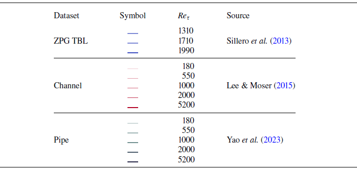


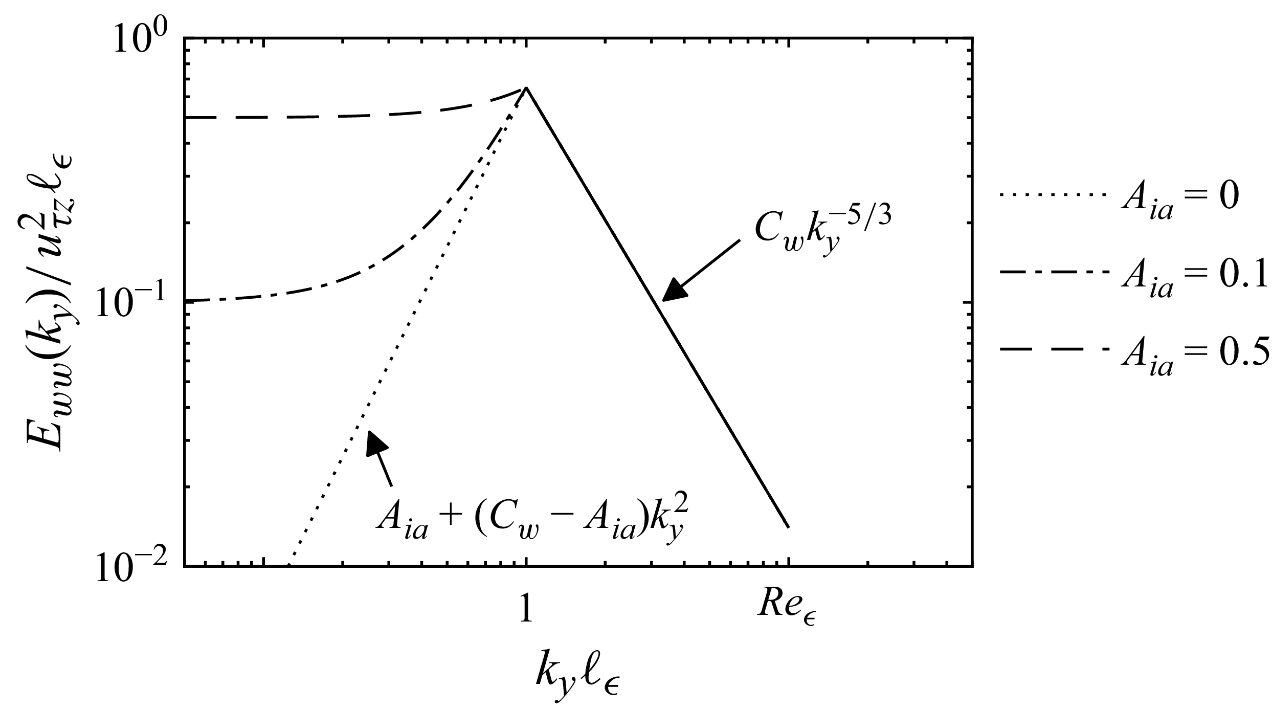


 Open access

