


1. Introduction
Schiller (Reference Schiller1922) outlined the concept for the determination of skin-friction losses in pipes of non-circular cross-sections based on the hydraulic diameter, $D_{h}=4A/P$
, and the Blasius (Reference Blasius1913) correlation for dimensionless coefficient of resistance,
$D_{h}=4A/P$
, and the Blasius (Reference Blasius1913) correlation for dimensionless coefficient of resistance, ${\it\lambda}={\rm\Delta}p/((1/2){\it\rho}U_{B}^{2})D_{h}/L=0.3164\mathit{Re}_{m}^{-0.25}$
, suggested originally to hold for pipes of circular cross-section. Here
${\it\lambda}={\rm\Delta}p/((1/2){\it\rho}U_{B}^{2})D_{h}/L=0.3164\mathit{Re}_{m}^{-0.25}$
, suggested originally to hold for pipes of circular cross-section. Here $A,P,{\rm\Delta}p,U_{B},{\it\rho},{\it\nu}$
and
$A,P,{\rm\Delta}p,U_{B},{\it\rho},{\it\nu}$
and $\mathit{Re}_{m}$
denote, respectively, pipe cross-sectional area, wetted perimeter, pressure drop over the pipe length
$\mathit{Re}_{m}$
denote, respectively, pipe cross-sectional area, wetted perimeter, pressure drop over the pipe length $L$
, bulk velocity, fluid density, kinematic viscosity of the fluid and Reynolds number
$L$
, bulk velocity, fluid density, kinematic viscosity of the fluid and Reynolds number $\mathit{Re}_{m}=D_{h}U_{B}/{\it\nu}$
. Using this correlation, Schiller succeeded in correlating the experimental data obtained in pipes of square, equilateral triangle and rectangular cross-sections in the Reynolds-number range up to
$\mathit{Re}_{m}=D_{h}U_{B}/{\it\nu}$
. Using this correlation, Schiller succeeded in correlating the experimental data obtained in pipes of square, equilateral triangle and rectangular cross-sections in the Reynolds-number range up to $\mathit{Re}_{m}\simeq 6\times 10^{4}$
. These findings were further supported by Nikuradse (Reference Nikuradse1930) for a wider class of cross-sectional geometries to form the basis for the determination of skin-friction losses in pipes of complex shapes. Minor modifications to this concept have been suggested (Idelchik Reference Idelchik1985), with marginal improvements for particular cross-sectional geometries (Jones Reference Jones1976).
$\mathit{Re}_{m}\simeq 6\times 10^{4}$
. These findings were further supported by Nikuradse (Reference Nikuradse1930) for a wider class of cross-sectional geometries to form the basis for the determination of skin-friction losses in pipes of complex shapes. Minor modifications to this concept have been suggested (Idelchik Reference Idelchik1985), with marginal improvements for particular cross-sectional geometries (Jones Reference Jones1976).
Resistance coefficient as a function of the Reynolds number measured by Schiller (Reference Schiller1922) in pipes of threaded and wavy cross-sections.

Schiller (Reference Schiller1922) pointed out that, for special geometries, deviations from the correlation based on the concept of hydraulic diameter might occur, and demonstrated this with results obtained in pipes of threaded and wavy cross-sections, as shown in figure 1. The notable increase in resistance above that expected is not surprising for pipes of threaded cross-section, since in addition to friction it includes the pressure drag, arising from non-orthogonality between the surface normal and the pipe axis, acting in a similar manner to the surface roughness. Figure 2 shows that, for pipes of wavy cross-section, the data lie below those expected, with a trend to deviate further with increasing Reynolds number. Such a trend implies that a wavy cross-section (in contrast to the cross-sectional geometries considered in figure 2) is capable of modifying the development of turbulent dissipation ${\it\epsilon}$
(II), which is expected (by an order-of-magnitude analysis) to prevail at large Reynolds numbers over the direct dissipation (I) originating from the mean flow. These two contributions to the energy dissipation form the total dissipation when integrated over the entire volume,
${\it\epsilon}$
(II), which is expected (by an order-of-magnitude analysis) to prevail at large Reynolds numbers over the direct dissipation (I) originating from the mean flow. These two contributions to the energy dissipation form the total dissipation when integrated over the entire volume, $V$
, of the moving fluid represent the average dissipation
$V$
, of the moving fluid represent the average dissipation $\overline{{\rm\Phi}}$
:
$\overline{{\rm\Phi}}$
:
 $$\begin{eqnarray}\overline{{\rm\Phi}}=\frac{1}{V}\int _{\!V}\,\underbrace{{\it\nu}\!\left(\frac{\partial \overline{U}_{i}}{\partial x_{j}}+\frac{\partial \overline{U}_{j}}{\partial x_{i}}\right)\!\frac{\partial \overline{U}_{i}}{\partial x_{j}}}_{\text{(I)}}+\underbrace{{\it\nu}\overline{\left(\frac{\partial u_{i}}{\partial x_{j}}+\frac{\partial u_{j}}{\partial x_{i}}\right)\!\frac{\partial u_{i}}{\partial x_{j}}}}_{\text{(II)},\,{\it\epsilon}}\,\text{d}V=\frac{A_{w}{\it\tau}_{w}U_{B}}{{\it\rho}V}.\end{eqnarray}$$
The average dissipation $\overline{{\rm\Phi}}$
can be interpreted as the work done against friction forces,
$\overline{{\rm\Phi}}$
can be interpreted as the work done against friction forces, $A_{w}{\it\tau}_{w}$
, per unit mass,
$A_{w}{\it\tau}_{w}$
, per unit mass, ${\it\rho}V$
, of the working fluid (where
${\it\rho}V$
, of the working fluid (where $A_{w}$
and
$A_{w}$
and ${\it\tau}_{w}={\it\nu}(\partial \overline{U}_{1}/\partial x_{2})_{w}$
are the wetted area and wall shear stress).
${\it\tau}_{w}={\it\nu}(\partial \overline{U}_{1}/\partial x_{2})_{w}$
are the wetted area and wall shear stress).
Experimental results for the resistance coefficient as a function of the Reynolds number from the original publication of Schiller (Reference Schiller1922) and data fits of ${\it\lambda}=a\mathit{Re}_{m}^{-b}$
for each pipe cross-sectional configuration.
${\it\lambda}=a\mathit{Re}_{m}^{-b}$
for each pipe cross-sectional configuration.

The aim of this work was to verify Schiller’s experimental results obtained in a pipe of wavy cross-section using direct numerical simulation. Of particular interest are: (i) the trend in the development of friction resistance with increasing Reynolds number; and (ii) anisotropy of turbulence and deviations from the statistically axisymmetric state along bisectors corresponding to the crest and valley regions of a wavy contour.
2. Laminar flow through pipes of square, triangular and wavy cross-sections
For numerical treatment of flows in pipes with complex geometries, the use of unstructured grids is desirable in conjunction with computer programs that offer great flexibility. Following such a plan, the wavy cross-sectional geometry from Schiller’s study was discretized in the original dimensions with unstructured cells using a grid generation program implemented in the numerical program STAR-CCM+ (http://www.cd-adapco.com/products/star-ccm-plus). The great advantage of unstructured cells was fully explored by automatic discretization of pipe cross-sections with polyhedral cells in the pipe core region, and prismatic cells for the near-wall region. This grid arrangement across the pipe cross-section is extended in the streamwise direction. Such a cell arrangement allows flexible mesh refinement at critical positions.
Figure 3 shows the grid generation of the wavy pipe cross-section employed in Schiller’s work. The structure of the grid cells is further elaborated in figure 4, showing details of the cell arrangement in the near-wall region.
(a) Cell generation for a pipe of wavy cross-section used for calculation of laminar and turbulent flow development; and (b) comparison of the wavy pipe contour with the contour of an Erlangen pipe from Lammers et al. (Reference Lammers, Jovanović, Frohnapfel and Delgado2012).

Non-structured grid arrangement generated for simulations of laminar and turbulent flow through a pipe of wavy cross-section (a) with enlarged detail (b).

Utilizing the generated grids, computations were performed with the numerical program OpenFOAM (http://www.openfoam.com). To evaluate the numerical accuracy, discretization errors were considered by carrying out computations for a few systematically refined grids. The results for the pressure gradient along the pipe, summarized in table 1, differ by less than 1 % and suggest that the numerical errors are fairly small. Computations for pipes of square and equilateral triangle-shaped cross-sections at $\mathit{Re}_{m}=500$
and
$\mathit{Re}_{m}=500$
and $\mathit{Re}_{m}=1000$
were found to differ from the corresponding analytical solutions (
$\mathit{Re}_{m}=1000$
were found to differ from the corresponding analytical solutions ( ${\it\lambda}=57/\mathit{Re}_{m}$
and
${\it\lambda}=57/\mathit{Re}_{m}$
and ${\it\lambda}=53/\mathit{Re}_{m}$
according to Schlichting Reference Schlichting1968) by only 0.2 % and 0.68 %, respectively.
${\it\lambda}=53/\mathit{Re}_{m}$
according to Schlichting Reference Schlichting1968) by only 0.2 % and 0.68 %, respectively.
3. Numerical methodology for simulation of turbulent flow through a wavy pipe
3.1. Computational flow domain
For numerical simulation of turbulent flow through a wavy pipe, the flow domain in the streamwise direction, $L_{x_{1}}$
, has to be chosen to capture flow features of prime importance. For the purpose of this study, these are the mean flow and to a lesser extent the second-order turbulence statistics. Since the flow is homogeneous in the streamwise direction, periodic boundary conditions were used along this direction.
$L_{x_{1}}$
, has to be chosen to capture flow features of prime importance. For the purpose of this study, these are the mean flow and to a lesser extent the second-order turbulence statistics. Since the flow is homogeneous in the streamwise direction, periodic boundary conditions were used along this direction.
Streamwise pressure gradient for a pipe of wavy cross-section for three different grid levels at $\mathit{Re}_{m}=1000$
.
$\mathit{Re}_{m}=1000$
.

The dependence of turbulence quantities on $L_{x_{1}}$
was analysed by Chin et al. (Reference Chin, Ooi, Marušić and Blackburn2010), who suggested a minimum computational pipe length for convergence of different turbulence statistics. Following the results from this study, we fixed
$L_{x_{1}}$
was analysed by Chin et al. (Reference Chin, Ooi, Marušić and Blackburn2010), who suggested a minimum computational pipe length for convergence of different turbulence statistics. Following the results from this study, we fixed $L_{x_{1}}=5D_{h}$
, which corresponds to
$L_{x_{1}}=5D_{h}$
, which corresponds to $L_{x_{1}}^{+}=L_{x_{1}}u_{{\it\tau}}/{\it\nu}=1700$
and
$L_{x_{1}}^{+}=L_{x_{1}}u_{{\it\tau}}/{\it\nu}=1700$
and $2150$
in viscous wall units (where
$2150$
in viscous wall units (where $u_{{\it\tau}}=({\it\tau}_{w}/{\it\rho})^{1/2}$
is the wall friction velocity) for simulations performed at
$u_{{\it\tau}}=({\it\tau}_{w}/{\it\rho})^{1/2}$
is the wall friction velocity) for simulations performed at $\mathit{Re}_{m}=4.5\times 10^{3}$
and
$\mathit{Re}_{m}=4.5\times 10^{3}$
and $10^{4}$
, respectively. This domain size ensures convergence of the mean flow for both Reynolds numbers and second-order statistics for
$10^{4}$
, respectively. This domain size ensures convergence of the mean flow for both Reynolds numbers and second-order statistics for $\mathit{Re}_{m}=10^{4}$
but not entirely for
$\mathit{Re}_{m}=10^{4}$
but not entirely for $\mathit{Re}_{m}=4.5\times 10^{3}$
(see Gavrilakis Reference Gavrilakis1992).
$\mathit{Re}_{m}=4.5\times 10^{3}$
(see Gavrilakis Reference Gavrilakis1992).
3.2. Spatial and temporal discretization
From previous studies of turbulence in wall-bounded flows (Grötzbach Reference Grötzbach1983; Wagner et al.
Reference Wagner, Hütel and Friedrich2001), it appears that very good agreement with experiments (if details that are not of great importance are omitted) can be achieved rationally by integrating the Navier–Stokes equations employing the finite-volume technique of second-order accuracy with an implicit integration scheme in time of the same accuracy by requiring resolutions of ${\rm\Delta}x_{1}=(5{-}6){\it\eta}_{K}$
in the streamwise direction and
${\rm\Delta}x_{1}=(5{-}6){\it\eta}_{K}$
in the streamwise direction and ${\rm\Delta}x_{2}={\rm\Delta}x_{3}=(2{-}3){\it\eta}_{K}$
in the normal and spanwise directions, with three or four points located within the region of the viscous sublayer, provided that the time step
${\rm\Delta}x_{2}={\rm\Delta}x_{3}=(2{-}3){\it\eta}_{K}$
in the normal and spanwise directions, with three or four points located within the region of the viscous sublayer, provided that the time step ${\rm\Delta}t$
is restricted by the value of the Courant number of 0.2:
${\rm\Delta}t$
is restricted by the value of the Courant number of 0.2:
 $$\begin{eqnarray}C={\rm\Delta}t\max \left|\frac{|u_{1}|}{{\rm\Delta}x_{1}}+\frac{|u_{2}|}{{\rm\Delta}x_{2}}+\frac{|u_{3}|}{{\rm\Delta}x_{3}}\right|\leqslant 0.2.\end{eqnarray}$$
Here ${\it\eta}_{K}=({\it\nu}^{3}/{\it\epsilon})^{1/4}$
corresponds to the Kolmogorov scale.
${\it\eta}_{K}=({\it\nu}^{3}/{\it\epsilon})^{1/4}$
corresponds to the Kolmogorov scale.
By estimating the value for ${\it\eta}_{K}$
,
${\it\eta}_{K}$
, ${\it\eta}_{K}^{+}=(0.25\mathit{Re}_{{\it\tau}}u_{{\it\tau}}/U_{B})^{1/2}$
with
${\it\eta}_{K}^{+}=(0.25\mathit{Re}_{{\it\tau}}u_{{\it\tau}}/U_{B})^{1/2}$
with $\mathit{Re}_{{\it\tau}}=u_{{\it\tau}}D_{h}/{\it\nu}$
, obtained from (1.1), the grid resolution of
$\mathit{Re}_{{\it\tau}}=u_{{\it\tau}}D_{h}/{\it\nu}$
, obtained from (1.1), the grid resolution of ${\rm\Delta}x_{1}^{+}=9.5$
,
${\rm\Delta}x_{1}^{+}=9.5$
, ${\rm\Delta}x_{2}^{+}={\rm\Delta}x_{3}^{+}=5$
was chosen for the flow core region and
${\rm\Delta}x_{2}^{+}={\rm\Delta}x_{3}^{+}=5$
was chosen for the flow core region and ${\rm\Delta}x_{2}^{+}={\rm\Delta}x_{3}^{+}=5/3$
for the region of the viscous sublayer. Using the Blasius correlation to estimate the magnitude of
${\rm\Delta}x_{2}^{+}={\rm\Delta}x_{3}^{+}=5/3$
for the region of the viscous sublayer. Using the Blasius correlation to estimate the magnitude of $O(u_{1})$
and assuming magnitudes
$O(u_{1})$
and assuming magnitudes $O(u_{2})=$ $O(u_{3})=u_{{\it\tau}}$
, a computational time step of
$O(u_{3})=u_{{\it\tau}}$
, a computational time step of ${\rm\Delta}t\leqslant 0.064{\it\nu}/u_{{\it\tau}}^{2}$
results from (3.1).
${\rm\Delta}t\leqslant 0.064{\it\nu}/u_{{\it\tau}}^{2}$
results from (3.1).
3.3. Initial conditions
For simulations of turbulence development in circular pipe flows, the starting field usually shows a tendency towards laminarization if numerical integration is started with random uncorrelated disturbances superimposed on a laminar solution or the universal law of the wall (Gavrilakis Reference Gavrilakis1992). In order to avoid laminarization and ensure development of turbulence, we initialized simulations as is done experimentally by tripping the flow at the pipe inlet with tripping plates or wires, which block the flow in the near-wall region to create conditions leading to the rapid development of turbulence (Schlichting Reference Schlichting1968). For a blockage ratio greater than 10 %, defined as the ratio of the blocked area to the pipe cross-sectional area, development towards the fully developed turbulent state (in a plane channel) is fairly rapid (Durst et al. Reference Durst, Fischer, Jovanović and Kikura1998; Fischer Reference Fischer1999).
Following experimental practice, we initialized simulations by blocking the flow across 15 % of the pipe cross-sectional area near the wall and specifying a uniform velocity distribution with random uncorrelated disturbances having a 10 % root mean square (r.m.s.) magnitude of $U_{B}$
across the rest of the pipe cross-section.
$U_{B}$
across the rest of the pipe cross-section.
4. Validation of the numerical procedure
To examine the adequacy of the applied numerical method and discretization, extensive studies were conducted by computing fully developed flows in a plane channel, circular pipe and square duct at low Reynolds numbers. For these canonical flows, reliable experimental data exist for the resistance coefficient as a function of the Reynolds number and also numerical results obtained with higher resolution compared with the present study by Kim et al. (Reference Kim, Moin and Moser1987) for a plane channel, Wu & Moin (Reference Wu and Moin2008) for a circular pipe and Gavrilakis (Reference Gavrilakis1992) and Lammers et al. (Reference Lammers, Jovanović, Frohnapfel and Delgado2012) for a square duct. Of special interest is the accuracy of the computed resistance coefficient, since the emphasis is placed on the influence of cross-sectional geometry on relaminarization of turbulence leading to drag reduction.
The computed ${\it\lambda}$
for plane channel flow at
${\it\lambda}$
for plane channel flow at $\mathit{Re}_{{\it\tau}}=180$
(where
$\mathit{Re}_{{\it\tau}}=180$
(where $\mathit{Re}_{{\it\tau}}={\it\delta}u_{{\it\tau}}/{\it\nu}$
is based on the channel half-height
$\mathit{Re}_{{\it\tau}}={\it\delta}u_{{\it\tau}}/{\it\nu}$
is based on the channel half-height ${\it\delta}$
) was found to be in very good agreement with Dean’s (Reference Dean1978) correlation and results obtained by Kim et al. (Reference Kim, Moin and Moser1987). For circular pipe flow at
${\it\delta}$
) was found to be in very good agreement with Dean’s (Reference Dean1978) correlation and results obtained by Kim et al. (Reference Kim, Moin and Moser1987). For circular pipe flow at $\mathit{Re}_{{\it\tau}}=Du_{{\it\tau}}/{\it\nu}=360$
, the difference between the numerical result for
$\mathit{Re}_{{\it\tau}}=Du_{{\it\tau}}/{\it\nu}=360$
, the difference between the numerical result for ${\it\lambda}$
and the value deduced from the Blasius correlation was within 1 %. Similar agreement was found for a square duct when compared with Jones’s (Reference Jones1976) correlation and simulations by Gavrilakis (Reference Gavrilakis1992).
${\it\lambda}$
and the value deduced from the Blasius correlation was within 1 %. Similar agreement was found for a square duct when compared with Jones’s (Reference Jones1976) correlation and simulations by Gavrilakis (Reference Gavrilakis1992).
Comparison of turbulent stresses in a plane channel flow with simulation results from (Kuroda Reference Kuroda1990). Stresses are normalized with the wall friction velocity $\overline{\unicode[STIX]{x1D636}_{i}\unicode[STIX]{x1D636}_{j}}^{+}=\overline{\unicode[STIX]{x1D636}_{i}\unicode[STIX]{x1D636}_{j}}/u_{{\it\tau}}^{2}$
and the wall distance
$\overline{\unicode[STIX]{x1D636}_{i}\unicode[STIX]{x1D636}_{j}}^{+}=\overline{\unicode[STIX]{x1D636}_{i}\unicode[STIX]{x1D636}_{j}}/u_{{\it\tau}}^{2}$
and the wall distance $x_{2}$
with
$x_{2}$
with $u_{{\it\tau}}$
and
$u_{{\it\tau}}$
and ${\it\nu}$
as
${\it\nu}$
as $x_{2}^{+}=u_{{\it\tau}}x_{2}/{\it\nu}$
.
$x_{2}^{+}=u_{{\it\tau}}x_{2}/{\it\nu}$
.

(a) The computational domain for simulations of turbulent flow through a square duct, and (b,c) comparisons of turbulent stresses for different domain lengths and computational cells with simulation results from Gavrilakis (Reference Gavrilakis1992).

To examine the capability of the employed numerical method, with details outlined in § 3, to resolve turbulence, figure 5 presents comparisons of the turbulent stresses $\overline{\unicode[STIX]{x1D636}_{i}\unicode[STIX]{x1D636}_{j}}$
in a fully developed plane channel flow with results obtained by Kuroda (Reference Kuroda1990) at
$\overline{\unicode[STIX]{x1D636}_{i}\unicode[STIX]{x1D636}_{j}}$
in a fully developed plane channel flow with results obtained by Kuroda (Reference Kuroda1990) at $\mathit{Re}_{{\it\tau}}=150$
using a pseudo-spectral numerical method. The good overall agreement of these results establishes confidence in the method employed for handling flows with complex wall boundaries involved in engineering.
$\mathit{Re}_{{\it\tau}}=150$
using a pseudo-spectral numerical method. The good overall agreement of these results establishes confidence in the method employed for handling flows with complex wall boundaries involved in engineering.
Further evidence supporting numerical issues in § 3 is presented in figure 6, which shows turbulent stresses in a fully developed flow through a square duct against the results obtained by Gavrilakis (Reference Gavrilakis1992). Apart from the good agreement between these results, the computations have a notable implication: independence of computed stresses from the computational cell arrangement and the length of the computational domain.
Supplementary validation was carried out by computing a fully developed flow through a triangular duct with small apex angle. Experiments performed by Eckert & Irvine (Reference Eckert and Irvine1956) showed laminarization of turbulence in the corner region of the duct and coexistence of laminar and fully developed turbulent regimes over a wide portion of the duct cross-section. The results of computations for the resistance coefficient ${\it\lambda}$
as a function of the Reynolds number
${\it\lambda}$
as a function of the Reynolds number $\mathit{Re}_{m}$
are shown in figure 7 along with those corresponding to experimental data. Very good agreement for all duct cross-sections is evident. The results for
$\mathit{Re}_{m}$
are shown in figure 7 along with those corresponding to experimental data. Very good agreement for all duct cross-sections is evident. The results for ${\it\lambda}$
show a tendency to fall below the Blasius correlation if the angle of the duct
${\it\lambda}$
show a tendency to fall below the Blasius correlation if the angle of the duct ${\it\alpha}$
is reduced. For a triangular duct with
${\it\alpha}$
is reduced. For a triangular duct with ${\it\alpha}=11.5^{\circ }$
, a constant reduction in
${\it\alpha}=11.5^{\circ }$
, a constant reduction in ${\it\lambda}$
of 20 % is seen over the entire turbulent regime investigated by Eckert & Irvine (Reference Eckert and Irvine1956).
${\it\lambda}$
of 20 % is seen over the entire turbulent regime investigated by Eckert & Irvine (Reference Eckert and Irvine1956).
Development of turbulent flow through a triangular duct (Daschiel, Frohnapfel & Jovanović Reference Daschiel, Frohnapfel and Jovanović2013). (a) Cross-section of the duct with (b) contour plot of the turbulent kinetic energy normalized with the wall friction velocity for a duct with ${\it\alpha}=11.5^{\circ }$
. (c) Comparisons of
${\it\alpha}=11.5^{\circ }$
. (c) Comparisons of ${\it\lambda}$
versus
${\it\lambda}$
versus $\mathit{Re}_{m}$
from measurements (open symbols) and computations (solid symbols) for different duct configurations: A, square duct, measurements from Hartnett et al. (Reference Hartnett, Koh and McComas1962); B, equilateral triangular duct, measurements from Nikuradse (Reference Nikuradse1930); C, triangular duct with
$\mathit{Re}_{m}$
from measurements (open symbols) and computations (solid symbols) for different duct configurations: A, square duct, measurements from Hartnett et al. (Reference Hartnett, Koh and McComas1962); B, equilateral triangular duct, measurements from Nikuradse (Reference Nikuradse1930); C, triangular duct with ${\it\alpha}=11.5^{\circ }$
, measurements from Eckert & Irvine (Reference Eckert and Irvine1956, Reference Eckert and Irvine1960); D, triangular duct with
${\it\alpha}=11.5^{\circ }$
, measurements from Eckert & Irvine (Reference Eckert and Irvine1956, Reference Eckert and Irvine1960); D, triangular duct with ${\it\alpha}=4^{\circ }$
, measurements from Carlson & Irvine (Reference Carlson and Irvine1961). (d) Anisotropy-invariant mapping of turbulence in a triangular duct with
${\it\alpha}=4^{\circ }$
, measurements from Carlson & Irvine (Reference Carlson and Irvine1961). (d) Anisotropy-invariant mapping of turbulence in a triangular duct with ${\it\alpha}=11.5^{\circ }$
: trajectories corresponding to different cross-sections
${\it\alpha}=11.5^{\circ }$
: trajectories corresponding to different cross-sections $0.25\leqslant x_{3}/H\leqslant 0.8$
indicate a tendency towards axisymmetry in the region of flow laminarization
$0.25\leqslant x_{3}/H\leqslant 0.8$
indicate a tendency towards axisymmetry in the region of flow laminarization $x_{3}/H\leqslant 0.3$
, which is followed by suppression of the turbulence development along the two-component state. Such an evolution of trajectories across the invariant map, in wall-bounded flows, implies a reduction of the turbulent dissipation rate at and away from the wall, leading to viscous drag reduction.
$x_{3}/H\leqslant 0.3$
, which is followed by suppression of the turbulence development along the two-component state. Such an evolution of trajectories across the invariant map, in wall-bounded flows, implies a reduction of the turbulent dissipation rate at and away from the wall, leading to viscous drag reduction.

The turbulence energy spectra of the streamwise velocity fluctuations at different locations along the $x_{3}$
axis of a triangular duct with
$x_{3}$
axis of a triangular duct with ${\it\alpha}=11.5^{\circ }$
normalized with Kolmogorov variables
${\it\alpha}=11.5^{\circ }$
normalized with Kolmogorov variables ${\it\eta}_{K}$
,
${\it\eta}_{K}$
, $u_{K}={\it\nu}/{\it\eta}_{K}$
and
$u_{K}={\it\nu}/{\it\eta}_{K}$
and $f_{K}=u_{K}/{\it\eta}_{K}$
: (a) time spectra; (b) spectra in the streamwise direction.
$f_{K}=u_{K}/{\it\eta}_{K}$
: (a) time spectra; (b) spectra in the streamwise direction.

For a triangular duct flow the energy spectra shown in figure 8 confirm that the resolution of simulation is sufficient since the energy associated with small scales is a few orders of magnitude smaller in comparison with the energy content at large scales. In the turbulence-dominated region near the triangle base, corresponding to $x_{3}/H=0.5$
and
$x_{3}/H=0.5$
and $x_{3}/H=0.7$
, the spectra collapse when scaled on the Kolmogorov’s variables, indicating that the spectral transfer is establishing (at very low
$x_{3}/H=0.7$
, the spectra collapse when scaled on the Kolmogorov’s variables, indicating that the spectral transfer is establishing (at very low $\mathit{Re}_{m}$
) towards features common for the turbulent energy cascade: in very narrow bands the spectra fall off as
$\mathit{Re}_{m}$
) towards features common for the turbulent energy cascade: in very narrow bands the spectra fall off as $-1$
and
$-1$
and $-5/3$
with increasing frequency or wavenumber. Approaching the corner region
$-5/3$
with increasing frequency or wavenumber. Approaching the corner region $x_{3}/H=0.3$
, where laminarization occurs, the spectra are significantly reduced, which results in a decrease of the turbulent dissipation rate
$x_{3}/H=0.3$
, where laminarization occurs, the spectra are significantly reduced, which results in a decrease of the turbulent dissipation rate ${\it\epsilon}$
and consequently in reduced spectral separation in the flow
${\it\epsilon}$
and consequently in reduced spectral separation in the flow $D_{h}/{\it\eta}_{K}$
. Anisotropy-invariant mapping of turbulence shown in figure 7(d) reveals that the laminarization process is accompanied by a tendency for turbulence to reach the statistically axisymmetric state, as discussed in § 5.2 and in more detail by Jovanović et al. (Reference Jovanović, Pashtrapanska, Frohnapfel, Durst, Koskinen and Koskinen2006a
,Reference Jovanović, Frohnapfel, Škaljić and Jovanović
b
).
$D_{h}/{\it\eta}_{K}$
. Anisotropy-invariant mapping of turbulence shown in figure 7(d) reveals that the laminarization process is accompanied by a tendency for turbulence to reach the statistically axisymmetric state, as discussed in § 5.2 and in more detail by Jovanović et al. (Reference Jovanović, Pashtrapanska, Frohnapfel, Durst, Koskinen and Koskinen2006a
,Reference Jovanović, Frohnapfel, Škaljić and Jovanović
b
).
5. Simulation results for turbulent flow through a wavy pipe
The computations were performed for two Reynolds numbers, $\mathit{Re}_{m}=4.5\times 10^{3}$
and
$\mathit{Re}_{m}=4.5\times 10^{3}$
and $\mathit{Re}_{m}=10^{4}$
.
$\mathit{Re}_{m}=10^{4}$
.
Starting from the initial field, equations were integrated in time until the field reached the statistically stationary state. By monitoring the development of the streamwise pressure gradient $\text{d}\overline{P}/\text{d}x_{1}$
, the stationary state was reached after approximately five turnover times of turbulence
$\text{d}\overline{P}/\text{d}x_{1}$
, the stationary state was reached after approximately five turnover times of turbulence $D_{h}/u_{{\it\tau}}$
. After the flow field had reached this state, equations were further integrated for an additional 20 turnover times to obtain averages of the statistical quantities of interest.
$D_{h}/u_{{\it\tau}}$
. After the flow field had reached this state, equations were further integrated for an additional 20 turnover times to obtain averages of the statistical quantities of interest.
Fourteen simulation runs were performed to study the influence of initial conditions and discretization errors on the flow development; a few runs were made at $\mathit{Re}_{m}=4.5\times 10^{3}$
with increased spatial resolution (compared with § 3.2) to examine the influence of discretization errors on the computed turbulence statistics, which turned out to be negligible for the quantities of interest. Only a selected sample of the computed results is presented, which provides synergy between theory, experiments and simulations, where computation results complement the description of the physical phenomena involved (Krieger Reference Krieger2012).
$\mathit{Re}_{m}=4.5\times 10^{3}$
with increased spatial resolution (compared with § 3.2) to examine the influence of discretization errors on the computed turbulence statistics, which turned out to be negligible for the quantities of interest. Only a selected sample of the computed results is presented, which provides synergy between theory, experiments and simulations, where computation results complement the description of the physical phenomena involved (Krieger Reference Krieger2012).
5.1. Influence of the Reynolds number on the resistance coefficient
We consider in some detail the influence of $\mathit{Re}_{m}$
on the pressure resistance coefficient
$\mathit{Re}_{m}$
on the pressure resistance coefficient ${\it\lambda}$
. In light of the data shown in figure 2 and considering (1.1), Schiller’s (Reference Schiller1922) results imply that a wavy cross-section decreases the turbulent dissipation rate,
${\it\lambda}$
. In light of the data shown in figure 2 and considering (1.1), Schiller’s (Reference Schiller1922) results imply that a wavy cross-section decreases the turbulent dissipation rate, $\overline{{\it\epsilon}}$
, as
$\overline{{\it\epsilon}}$
, as $\mathit{Re}_{m}$
increases. Such a tendency is favourable for achieving turbulent drag reduction. The possibility that turbulence can be altered by the pipe cross-sectional geometry was recently proposed by our group using the tools of the invariant theory and by exploring numerical databases of wall-bounded flows. In the context of the above-mentioned work, Schiller’s experimental results provide proof of the concept that we termed the ‘Erlangen pipe’ (Lammers et al.
Reference Lammers, Jovanović, Frohnapfel and Delgado2012).
$\mathit{Re}_{m}$
increases. Such a tendency is favourable for achieving turbulent drag reduction. The possibility that turbulence can be altered by the pipe cross-sectional geometry was recently proposed by our group using the tools of the invariant theory and by exploring numerical databases of wall-bounded flows. In the context of the above-mentioned work, Schiller’s experimental results provide proof of the concept that we termed the ‘Erlangen pipe’ (Lammers et al.
Reference Lammers, Jovanović, Frohnapfel and Delgado2012).
Initial attempts to reproduce Schiller’s experimental result for ${\it\lambda}$
at
${\it\lambda}$
at $\mathit{Re}_{m}=4.5\times 10^{3}$
revealed strong damping of turbulence by the wavy cross-section, which led after a few turnover times to complete flow relaminarization. Only with significant tripping of the initial flow, by blocking the flow over 30 % of the pipe cross-sectional area, was it possible to realize a fully developed turbulent state with the pressure resistance coefficient in very close agreement with experiments (see table 2).
$\mathit{Re}_{m}=4.5\times 10^{3}$
revealed strong damping of turbulence by the wavy cross-section, which led after a few turnover times to complete flow relaminarization. Only with significant tripping of the initial flow, by blocking the flow over 30 % of the pipe cross-sectional area, was it possible to realize a fully developed turbulent state with the pressure resistance coefficient in very close agreement with experiments (see table 2).
Unlike the simulation performed at $\mathit{Re}_{m}=4.5\times 10^{3}$
, a fully developed turbulent state for
$\mathit{Re}_{m}=4.5\times 10^{3}$
, a fully developed turbulent state for $\mathit{Re}_{m}=10^{4}$
was achieved by blocking the initial flow over a much smaller portion (15 %) of the pipe cross-sectional area. Table 2 and figure 9 show that the computational results obtained for
$\mathit{Re}_{m}=10^{4}$
was achieved by blocking the initial flow over a much smaller portion (15 %) of the pipe cross-sectional area. Table 2 and figure 9 show that the computational results obtained for ${\it\lambda}$
agree fairly well with Schiller’s experimental findings and therefore support the trend in the data in figure 2 as
${\it\lambda}$
agree fairly well with Schiller’s experimental findings and therefore support the trend in the data in figure 2 as $\mathit{Re}_{m}$
increases, which implies a potential for turbulent drag reduction.
$\mathit{Re}_{m}$
increases, which implies a potential for turbulent drag reduction.
Variation of ${\it\lambda}$
against
${\it\lambda}$
against $\mathit{Re}_{m}$
for a wavy pipe cross-section: comparisons between experiments and simulations.
$\mathit{Re}_{m}$
for a wavy pipe cross-section: comparisons between experiments and simulations.

Comparison of simulation and experimental results for the resistance coefficients in a wavy pipe.
The CPU time required for simulation of flow at $\mathit{Re}_{m}=10^{4}$
was approximately 1200 h. Calculations were processed in parallel utilizing 128 processors of the Woodcrest Cluster of the Erlangen Regional Computer Center, which has an overall peak performance of
$\mathit{Re}_{m}=10^{4}$
was approximately 1200 h. Calculations were processed in parallel utilizing 128 processors of the Woodcrest Cluster of the Erlangen Regional Computer Center, which has an overall peak performance of $10.4\ \text{Tflop}\ \text{s}^{-1}$
(
$10.4\ \text{Tflop}\ \text{s}^{-1}$
( $6.62\ \text{Tflop}\ \text{s}^{-1}$
LINPACK). The enormous demand for required CPU time prevented computations at higher Reynolds numbers.
$6.62\ \text{Tflop}\ \text{s}^{-1}$
LINPACK). The enormous demand for required CPU time prevented computations at higher Reynolds numbers.
5.2. Anisotropy-invariant mapping of turbulence and its implications
In order to elucidate the mechanism responsible for the reduction of ${\it\lambda}$
(and therefore
${\it\lambda}$
(and therefore $\overline{{\it\epsilon}}$
) below the level expected from the Blasius correlation, anisotropy-invariant mapping of turbulence was performed along bisectors of the wavy pipe cross-section. Analytic considerations based on the equations for the mean flow led to the conclusion that turbulence in wall-bounded flows can be completely suppressed if it is forced towards the statistically axisymmetric state, resulting in significant reductions of
$\overline{{\it\epsilon}}$
) below the level expected from the Blasius correlation, anisotropy-invariant mapping of turbulence was performed along bisectors of the wavy pipe cross-section. Analytic considerations based on the equations for the mean flow led to the conclusion that turbulence in wall-bounded flows can be completely suppressed if it is forced towards the statistically axisymmetric state, resulting in significant reductions of $\overline{{\it\epsilon}}$
and
$\overline{{\it\epsilon}}$
and ${\it\lambda}$
.
${\it\lambda}$
.
The above fundamental deduction, which is supported by all databases from direct numerical simulations (Frohnapfel et al. Reference Frohnapfel, Lammers, Jovanović and Durst2007a ), logically follows from the Reynolds equations for the mean flow,
 $$\begin{eqnarray}\frac{\partial \overline{U}_{i}}{\partial t}+\overline{U}_{k}\frac{\partial \overline{U}_{i}}{\partial x_{k}}=-\frac{1}{{\it\rho}}\frac{\partial \overline{P}}{\partial x_{i}}+\frac{\partial }{\partial x_{k}}\!\left[{\it\nu}\frac{\partial \overline{U}_{i}}{\partial x_{k}}-\overline{\unicode[STIX]{x1D636}_{i}\unicode[STIX]{x1D636}_{k}}\right],\quad i,k=1,2,3,\end{eqnarray}$$
in simple parallel wall-bounded flows, by demanding statistical axisymmetry in the turbulent stress tensor $\overline{\unicode[STIX]{x1D636}_{i}\unicode[STIX]{x1D636}_{j}}=A{\it\delta}_{ij}+B\boldsymbol{k}_{i}\boldsymbol{k}_{j}$
, where
$\overline{\unicode[STIX]{x1D636}_{i}\unicode[STIX]{x1D636}_{j}}=A{\it\delta}_{ij}+B\boldsymbol{k}_{i}\boldsymbol{k}_{j}$
, where $A$
and
$A$
and $B$
are scalar functions and
$B$
are scalar functions and $\boldsymbol{k}_{i}$
is the unit vector defined in such a way that
$\boldsymbol{k}_{i}$
is the unit vector defined in such a way that $\overline{\unicode[STIX]{x1D636}_{i}\unicode[STIX]{x1D636}_{j}}$
is invariant under rotation about the axis defined by its scalar arguments, say
$\overline{\unicode[STIX]{x1D636}_{i}\unicode[STIX]{x1D636}_{j}}$
is invariant under rotation about the axis defined by its scalar arguments, say $\boldsymbol{k}_{i}=(1,0,0)$
. For such a stress configuration, (5.1) transforms from unclosed to closed form:
$\boldsymbol{k}_{i}=(1,0,0)$
. For such a stress configuration, (5.1) transforms from unclosed to closed form:
 $$\begin{eqnarray}\frac{\partial \overline{U}_{i}}{\partial t}+\overline{U}_{k}\frac{\partial \overline{U}_{i}}{\partial x_{k}}=-\frac{1}{{\it\rho}}\frac{\partial }{\partial x_{i}}\,\underbrace{\left(\overline{P}+\frac{1}{3}{\it\rho}q^{2}+\frac{2}{3}{\it\rho}B\right)}_{\text{modified}\,\text{pressure}\,P^{\ast }}+\,{\it\nu}\frac{\partial ^{2}\overline{U}_{i}}{\partial x_{k}\partial x_{k}},\quad i,k=1,2,3,\end{eqnarray}$$
where $q^{2}$
denotes the trace of
$q^{2}$
denotes the trace of $\overline{\unicode[STIX]{x1D636}_{i}\unicode[STIX]{x1D636}_{j}}$
. For fully developed flow, (5.2) obviously leads to solutions that coincide with the corresponding solutions for laminar flows. From these results, it appears that statistical axisymmetry in the turbulent stresses leads to flow relaminarization and therefore to a large viscous drag reduction effect.
$\overline{\unicode[STIX]{x1D636}_{i}\unicode[STIX]{x1D636}_{j}}$
. For fully developed flow, (5.2) obviously leads to solutions that coincide with the corresponding solutions for laminar flows. From these results, it appears that statistical axisymmetry in the turbulent stresses leads to flow relaminarization and therefore to a large viscous drag reduction effect.
Anisotropy-invariant mapping of turbulence in a wavy pipe cross-section: trajectories along (a) the crest region and (b) the valley region display substantially different flow behaviour, which can be readily seen in the distribution of the turbulence energy production (c).

Distributions of turbulent stresses along (a) valley and (b) crest bisectors of the wavy pipe and comparisons with the stress distributions in a square duct.

Turbulence energy spectra of the streamwise velocity fluctuations across a wavy pipe cross-section. Distributions correspond to locations on crest and valley bisectors measured from the pipe centreline $r$
relative to distance
$r$
relative to distance $r_{B}$
from the pipe centreline up to the wall: (a,b) time spectra; (c,d) spectra in the streamwise direction.
$r_{B}$
from the pipe centreline up to the wall: (a,b) time spectra; (c,d) spectra in the streamwise direction.

Figure 10 shows that trajectories across the anisotropy-invariant map, constructed from invariants of the anisotropy tensor, $\unicode[STIX]{x1D622}_{ij}=\overline{\unicode[STIX]{x1D636}_{i}\unicode[STIX]{x1D636}_{j}}/q^{2}-{\it\delta}_{ij}/3$
,
$\unicode[STIX]{x1D622}_{ij}=\overline{\unicode[STIX]{x1D636}_{i}\unicode[STIX]{x1D636}_{j}}/q^{2}-{\it\delta}_{ij}/3$
, $\text{II}_{a}=\unicode[STIX]{x1D622}_{ij}\unicode[STIX]{x1D622}_{ji}$
and
$\text{II}_{a}=\unicode[STIX]{x1D622}_{ij}\unicode[STIX]{x1D622}_{ji}$
and $\text{III}_{a}=\unicode[STIX]{x1D622}_{ij}\unicode[STIX]{x1D622}_{jk}\unicode[STIX]{x1D622}_{ki}$
, along bisectors corresponding to the crest and valley regions of a wavy pipe cross-section are substantially different. This figure also includes the distribution of the production of turbulence kinetic energy
$\text{III}_{a}=\unicode[STIX]{x1D622}_{ij}\unicode[STIX]{x1D622}_{jk}\unicode[STIX]{x1D622}_{ki}$
, along bisectors corresponding to the crest and valley regions of a wavy pipe cross-section are substantially different. This figure also includes the distribution of the production of turbulence kinetic energy $P_{k}=-\overline{\unicode[STIX]{x1D636}_{i}\unicode[STIX]{x1D636}_{k}}\,\partial \overline{U_{i}}/\partial x_{k}$
across a wavy pipe cross-section in order to provide an understanding of the influence of anisotropy on the generation of
$P_{k}=-\overline{\unicode[STIX]{x1D636}_{i}\unicode[STIX]{x1D636}_{k}}\,\partial \overline{U_{i}}/\partial x_{k}$
across a wavy pipe cross-section in order to provide an understanding of the influence of anisotropy on the generation of $P_{k}$
.
$P_{k}$
.
The trajectory corresponding to the crest bisector shows that turbulence in this region develops along the two-component state near the wall and deviates from the axisymmetric state away from the wall. Analysis of such turbulence shows that it permanently destabilizes the flow owing to promotion of the turbulent dissipation generated initially at the wall and subsequently developing away from the wall, which enables self-maintenance of the turbulent state.
The trajectory corresponding to the valley region coincides with the boundary of the anisotropy map, which corresponds to the statistically axisymmetric state. In light of (5.1) and (5.2), it is not surprising that turbulence is strongly reduced and even entirely suppressed across the entire valley region of the wavy cross-section.
Distributions of turbulence stresses along bisectors corresponding to valley and crest regions shown in figure 11 preserve the same character as the stresses along corner and wall normal bisectors of a square pipe. Reduction of the turbulence level along the valley bisector where turbulence reaches an almost statistically axisymmetric state is substantial.
Spectral distributions, shown in figure 12, further elucidate the turbulence development along two characteristic bisectors of a wavy pipe cross-section. No noticeable effect on the energy transfer can be observed when approaching the pipe centreline from different radial directions. This, however, is altered on moving towards the pipe wall, where a significant reduction in the energy content can be observed across the valley region. This is in agreement with deductions made from anisotropy-invariant mapping shown in figure 10 and from the analysis involving (5.1) and (5.2) by exploring the concept of statistical axisymmetry.
Turbulent dissipation rate at the wall, ${\it\epsilon}_{wall}$
, normalized with
${\it\epsilon}_{wall}$
, normalized with $u_{{\it\tau}}$
and
$u_{{\it\tau}}$
and ${\it\nu}$
versus the anisotropy of turbulence
${\it\nu}$
versus the anisotropy of turbulence $\text{II}_{a}$
at the wall extracted from available numerical databases. A best fit through the numerical data extrapolates well the trend predicted by Jovanović & Hillerbrand (Reference Jovanović and Hillerbrand2005) as the one-component limit
$\text{II}_{a}$
at the wall extracted from available numerical databases. A best fit through the numerical data extrapolates well the trend predicted by Jovanović & Hillerbrand (Reference Jovanović and Hillerbrand2005) as the one-component limit $(\text{II}_{a}=2/3)$
is approached. Amplification of the kinetic energy of turbulence
$(\text{II}_{a}=2/3)$
is approached. Amplification of the kinetic energy of turbulence $k$
close to the wall is in the direction of the sketched arrow.
$k$
close to the wall is in the direction of the sketched arrow.

From the distribution of $P_{k}$
shown in figure 10 and results presented in figures 11 and 12, it appears that the underlying physical mechanism responsible for self-maintenance and suppression of turbulence across a wavy pipe cross-section is localized in the region very close to the pipe wall. Therefore, the necessary understanding of this process can be inferred from the asymptotic behaviour of the velocity fluctuations near the wall enforced to satisfy the continuity equation for the instantaneous fluctuations
$P_{k}$
shown in figure 10 and results presented in figures 11 and 12, it appears that the underlying physical mechanism responsible for self-maintenance and suppression of turbulence across a wavy pipe cross-section is localized in the region very close to the pipe wall. Therefore, the necessary understanding of this process can be inferred from the asymptotic behaviour of the velocity fluctuations near the wall enforced to satisfy the continuity equation for the instantaneous fluctuations $\partial u_{i}/\partial x_{i}=0$
,
$\partial u_{i}/\partial x_{i}=0$
,
 $$\begin{eqnarray}\left.\begin{array}{@{}rcr@{}}u_{1} & = & a_{1}x_{2}+a_{2}x_{2}^{2}+\cdots \\ u_{2} & = & +\,b_{2}x_{2}^{2}+\cdots \\ u_{3} & = & c_{1}x_{2}+c_{2}x_{2}^{2}+\cdots \end{array}\right\}\quad \text{as}\ x_{2}\rightarrow 0,\end{eqnarray}$$
to yield the asymptotic behaviour of turbulent stresses and the dissipation rate near the wall,
 $$\begin{eqnarray}\left.\begin{array}{@{}rcl@{}}\overline{u_{1}^{2}} & = & \overline{a_{1}^{2}}x_{2}^{2}+\cdots \\ \overline{u_{2}^{2}} & = & \overline{b_{2}^{2}}x_{2}^{4}+\cdots \\ \overline{u_{3}^{2}} & = & \overline{c_{1}^{2}}x_{2}^{2}+\cdots \\ {\it\epsilon} & = & {\it\nu}(\overline{a_{1}^{2}}+\overline{c_{1}^{2}})+\cdots \end{array}\right\}\quad \text{as}\ x_{2}\rightarrow 0.\end{eqnarray}$$
The above results lead to the conclusion that the kinetic energy of turbulence $k=\overline{\unicode[STIX]{x1D636}_{i}\unicode[STIX]{x1D636}_{i}}/2$
increases in proportion to the magnitude of the dissipation rate at the wall
$k=\overline{\unicode[STIX]{x1D636}_{i}\unicode[STIX]{x1D636}_{i}}/2$
increases in proportion to the magnitude of the dissipation rate at the wall $({\it\epsilon})_{wall}={\it\nu}(\overline{a_{1}^{2}}+\overline{c_{1}^{2}})$
:
$({\it\epsilon})_{wall}={\it\nu}(\overline{a_{1}^{2}}+\overline{c_{1}^{2}})$
:
 $$\begin{eqnarray}k=\frac{1}{2}\frac{({\it\epsilon})_{wall}}{{\it\nu}}x_{2}^{2}+\cdots \,.\end{eqnarray}$$
This suggests that turbulence can be entirely suppressed, leading to flow laminarization, if and only if ${\it\epsilon}_{wall}\rightarrow 0$
. The behaviour of
${\it\epsilon}_{wall}\rightarrow 0$
. The behaviour of ${\it\epsilon}_{wall}$
as a function of turbulence anisotropy at the wall
${\it\epsilon}_{wall}$
as a function of turbulence anisotropy at the wall $(\text{II}_{a})_{wall}$
, shown in figure 13, reveals that
$(\text{II}_{a})_{wall}$
, shown in figure 13, reveals that ${\it\epsilon}_{wall}$
decreases monotonically with increasing anisotropy and vanishes at the one-component state, which is the state of maximum anisotropy. We conclude from (5.5) and figures 10 and 13 that production of turbulence in the crest region and damping of turbulence and flow laminarization in the valley region of a wavy pipe cross-section are logical and not surprising considering the evolution of anisotropies near the wall, which lie on the two-component boundary of the anisotropy map as shown in figure 10(a,b).
${\it\epsilon}_{wall}$
decreases monotonically with increasing anisotropy and vanishes at the one-component state, which is the state of maximum anisotropy. We conclude from (5.5) and figures 10 and 13 that production of turbulence in the crest region and damping of turbulence and flow laminarization in the valley region of a wavy pipe cross-section are logical and not surprising considering the evolution of anisotropies near the wall, which lie on the two-component boundary of the anisotropy map as shown in figure 10(a,b).
5.3. Suppression of the turbulence development by wavy cross-section
The above-discussed evidence suggests the possibility of modulating the essential features of turbulence ( $\overline{{\it\epsilon}}$
) by the wall topology and in this way stabilize the laminar flow development if axisymmetry in the disturbances across the valley region prevail over the crest region and expand to the entire pipe cross-section. For the original pipe configuration used by Schiller (Reference Schiller1922), this might be possible, but only under special circumstances, which must be considered as exceptional and not the rule.
$\overline{{\it\epsilon}}$
) by the wall topology and in this way stabilize the laminar flow development if axisymmetry in the disturbances across the valley region prevail over the crest region and expand to the entire pipe cross-section. For the original pipe configuration used by Schiller (Reference Schiller1922), this might be possible, but only under special circumstances, which must be considered as exceptional and not the rule.
Segment of the cross-sectional plane of a wavy pipe with a cylindrical coordinate system and bisectors corresponding to crest ( $r_{B}$
) and valley (
$r_{B}$
) and valley ( $R_{b}$
) regions. Circular arcs at positions
$R_{b}$
) regions. Circular arcs at positions $r/r_{B}=0.9$
(square symbol),
$r/r_{B}=0.9$
(square symbol), $r/r_{B}=0.95$
(circle symbol),
$r/r_{B}=0.95$
(circle symbol), $r/r_{B}=0.99$
(rectangle symbol) and
$r/r_{B}=0.99$
(rectangle symbol) and $B(r)$
denotes the length of a circular arc.
$B(r)$
denotes the length of a circular arc.

Analysis of velocity profiles in the radial direction: profiles along crest and valley regions in (a) laminar and (b) turbulent flow regimes; (c) first derivative $\partial U_{z}/\partial r$
and (d) second derivative
$\partial U_{z}/\partial r$
and (d) second derivative $\partial ^{2}U_{z}/\partial r^{2}$
of the profiles shown at the top. There is no sign of inflectional instability
$\partial ^{2}U_{z}/\partial r^{2}$
of the profiles shown at the top. There is no sign of inflectional instability $\partial ^{2}U_{z}/\partial r^{2}=0$
for the laminar velocity profile.
$\partial ^{2}U_{z}/\partial r^{2}=0$
for the laminar velocity profile.
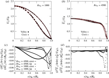
Owing to the complex shape of the cross-sectional geometry, the velocity profiles in a wavy pipe exhibit curvature with inflection points. Such profiles are inviscidly unstable and are suspected to lead to the rapid production of turbulence (Gupta, Laufer & Kaplan Reference Gupta, Laufer and Kaplan1971; Blackwelder & Kaplan Reference Blackwelder and Kaplan1976; Blackwelder Reference Blackwelder1989). As long as axisymmetry in the turbulence stresses $\overline{\unicode[STIX]{x1D636}_{i}\unicode[STIX]{x1D636}_{j}}$
prevails, such instability cannot develop owing to (5.2). Away from the valley and towards the crest region, axisymmetry is not preserved and development of turbulence is expected, as can be seen for the results shown in figure 10(c). Analysis of velocity profiles along radial and tangential directions carried out for the laminar (
$\overline{\unicode[STIX]{x1D636}_{i}\unicode[STIX]{x1D636}_{j}}$
prevails, such instability cannot develop owing to (5.2). Away from the valley and towards the crest region, axisymmetry is not preserved and development of turbulence is expected, as can be seen for the results shown in figure 10(c). Analysis of velocity profiles along radial and tangential directions carried out for the laminar ( $\mathit{Re}_{m}=1000$
) and turbulent (
$\mathit{Re}_{m}=1000$
) and turbulent ( $\mathit{Re}_{m}=4500$
) flow regimes shown in figures 15 and 16 reveal that the appearance of instability is likely to start along the tangential direction (Holmes et al.
Reference Holmes, Lumley and Berkooz1996) and is more critical for turbulent than for laminar flow conditions. These results hold promise in attempts to maintain the laminar regime in a wavy pipe under circumstances that lead to the appearance of turbulence in pipes of circular cross-section.
$\mathit{Re}_{m}=4500$
) flow regimes shown in figures 15 and 16 reveal that the appearance of instability is likely to start along the tangential direction (Holmes et al.
Reference Holmes, Lumley and Berkooz1996) and is more critical for turbulent than for laminar flow conditions. These results hold promise in attempts to maintain the laminar regime in a wavy pipe under circumstances that lead to the appearance of turbulence in pipes of circular cross-section.
Analysis of velocity profiles in the tangential direction: profiles for (a) laminar and (b) turbulent flow regimes; (c) first derivative $\partial U_{z}/\partial {\it\phi}$
and (d) second derivative
$\partial U_{z}/\partial {\it\phi}$
and (d) second derivative $\partial ^{2}U_{z}/\partial {\it\phi}^{2}$
of profiles shown at the top. There is weak evidence of inflectional instability
$\partial ^{2}U_{z}/\partial {\it\phi}^{2}$
of profiles shown at the top. There is weak evidence of inflectional instability $\partial ^{2}U_{z}/\partial {\it\phi}^{2}$
for laminar flow.
$\partial ^{2}U_{z}/\partial {\it\phi}^{2}$
for laminar flow.

This approach was applied in previous work on fully developed turbulent channel flows and promising results were obtained by: (i) virtual forcing of the axisymmetric state in the region close to the wall (Frohnapfel et al.
Reference Frohnapfel, Lammers, Jovanović and Durst2007a
); (ii) using surface-embedded grooves to produce turbulent drag reduction by flow laminarization (Frohnapfel, Jovanović & Delgado Reference Frohnapfel, Jovanović and Delgado2007b
); and (iii) employing microgroove surface topology to stabilize the laminar boundary layer development (Jovanović et al.
Reference Jovanović, Frohnapfel, Srikantharajah, Jovanović, Lienhart and Delgado2011). Following the results of these studies, we decided to carry out parallel simulations of the flow development in pipes of circular and wavy cross-sections with the same initial conditions corresponding to flow blockage over 15 % of the pipe cross-sectional area at $\mathit{Re}_{m}=4.95\times 10^{3}$
.
$\mathit{Re}_{m}=4.95\times 10^{3}$
.
Time development of the streamwise pressure gradient normalized with the corresponding value for the laminar flow regime as a function of the turnover time of turbulence for pipes of circular and wavy cross sections for $\mathit{Re}_{m}=4.95\times 10^{3}$
and the same level of flow blockage corresponding to 15 % of the pipe cross-sectional area.
$\mathit{Re}_{m}=4.95\times 10^{3}$
and the same level of flow blockage corresponding to 15 % of the pipe cross-sectional area.

Comparison of the pressure resistance coefficients for pipes of circular and wavy cross-sections for the same level of flow blockage corresponding to 15 % of the pipe cross-sectional area.
Simulation results revealed that the cross-sectional geometry of a wavy pipe used by Schiller (Reference Schiller1922) was resistant to the appearance of transition and did not show any sign of onset of turbulence, which was not the case, however, for the circular pipe, where turbulence was fully developed after just a few turnover times. Table table 3 summarizes computational results showing significant differences in ${\it\lambda}$
for two different cross-sectional configurations and figure 17 emphasizes the huge gain in terms of viscous drag reduction of
${\it\lambda}$
for two different cross-sectional configurations and figure 17 emphasizes the huge gain in terms of viscous drag reduction of $DR\approx 66\,\%$
.
$DR\approx 66\,\%$
.
Turbulence development in pipes of non-circular cross-section. Note that the minimum in $P_{k}$
corresponds to the Erlangen design shown in panel (c).
$P_{k}$
corresponds to the Erlangen design shown in panel (c).

6. Conclusions
Direct numerical simulation of turbulent flow through a pipe of wavy cross-section confirmed experimental results obtained by Schiller (Reference Schiller1922), which display the trend in the resistance coefficient ${\it\lambda}$
to fall below the level that is expected to hold universally for pipes with non-circular cross-sections. These findings are supported by anisotropy-invariant mapping of turbulence and supplementary calculations aimed at simulating onset and breakdown to fully developed turbulence in pipes of different cross-sectional configurations.
${\it\lambda}$
to fall below the level that is expected to hold universally for pipes with non-circular cross-sections. These findings are supported by anisotropy-invariant mapping of turbulence and supplementary calculations aimed at simulating onset and breakdown to fully developed turbulence in pipes of different cross-sectional configurations.
An interpretation based on the manner in which wavy cross-sectional geometry modulates near-wall turbulence leads to the conclusion that Schiller’s experimental results and complementary numerical simulations support the concept of the ‘Erlangen pipe’ developed by the authors, which forces near-wall turbulence to approach the state when it must be completely suppressed, leading to significant viscous drag reduction (Lammers et al. Reference Lammers, Jovanović, Frohnapfel and Delgado2012). Implications of the above work for drag reduction and control of laminar to turbulence transition at high Reynolds number are the subject of current research efforts, as illustrated in figure 18.
Acknowledgements
This paper was an integral part of projects Jo 240/9-1 and Jo 240/10-1 submitted for funding to Deutsche Forschungsgemeinschaft with Dr M. Lentze acting as the technical monitor.


 Open access