


1. Introduction
Many systems with complex, multiscale structure are nevertheless characterized by emergent large-scale coherence (Haken Reference Haken1983; Cross & Hohenberg Reference Cross and Hohenberg1993), generating low-dimensional structure often conceptualized as an attracting or slow manifold. This phenomenon is especially relevant in fluid dynamics, where successive bifurcations lead to increasingly complex behaviour and eventually the transition to turbulence (Landau Reference Landau1944; Stuart Reference Stuart1958; Lorenz Reference Lorenz1963; Ruelle & Takens Reference Ruelle and Takens1971; Swinney & Gollub Reference Swinney and Gollub1981). Dynamical models that capture this intrinsic low-dimensional structure can improve our physical understanding and are critical for real-time optimization and control objectives (Noack, Morzynski & Tadmor Reference Noack, Morzynski and Tadmor2011; Brunton & Noack Reference Brunton and Noack2015; Rowley & Dawson Reference Rowley and Dawson2017).
Close to a bifurcation, the dynamics is approximately restricted to the manifold described by the amplitudes of the unstable eigenmodes. The evolution equations for these effective coordinates are given by the normal form for the bifurcation (Guckenheimer & Holmes Reference Guckenheimer and Holmes1983), the form of which can be deduced with symmetry arguments (Golubitsky & Langford Reference Golubitsky and Langford1988; Glaz et al. Reference Glaz, Mezić, Fonoberova and Loire2017; Deng et al. Reference Deng, Noack, Morzynski and Pastur2020), weakly nonlinear analysis (Stuart Reference Stuart1958; Sipp & Lebedev Reference Sipp and Lebedev2007; Meliga, Chomaz & Sipp Reference Meliga, Chomaz and Sipp2009), or a centre manifold reduction (Carini, Auteri & Giannetti Reference Carini, Auteri and Giannetti2015). Normal forms can describe a wide range of stereotypical dynamics, including bistability, self-sustained oscillations and chaos.
These arguments are only valid near the bifurcation, although empirical methods can generalize this approach beyond the point where models can be derived via asymptotic expansions. These methods typically represent the field as a linear combination of modes (Taira et al. Reference Taira, Brunton, Dawson, Rowley, Colonius, McKeon, Schmidt, Gordeyev, Theofilis and Ukeiley2017), followed by either Galerkin projection onto the governing equations (Aubry et al. Reference Aubry, Holmes, Lumley and Stone1988; Holmes, Lumley & Berkooz Reference Holmes, Lumley and Berkooz1996; Noack et al. Reference Noack, Afanasiev, Morzyński, Tadmor and Thiele2003, Reference Noack, Morzynski and Tadmor2011), data-driven system identification (Brunton, Proctor & Kutz Reference Brunton, Proctor and Kutz2016; Loiseau & Brunton Reference Loiseau and Brunton2018; Loiseau Reference Loiseau2020; Rubini, Lasagna & Da Ronch Reference Rubini, Lasagna and Da Ronch2020) or a hybrid of the two (Mohebujjaman, Rebholz & Iliescu Reference Mohebujjaman, Rebholz and Iliescu2018; Xie et al. Reference Xie, Mohebujjaman, Rebholz and Iliescu2018).
A linear modal basis is typically derived as the solution to some optimization problem. For example, proper orthogonal decomposition (POD) modes minimize the kinetic energy of the unresolved fluctuations for a given basis size, with the residual monotonically decreasing with the basis dimensionality (Holmes et al. Reference Holmes, Lumley and Berkooz1996). On the other hand, dynamic mode decomposition (DMD) incorporates temporal information via the spectral decomposition of a best-fit linear evolution operator that advances the flow measurements forward in time (Rowley et al. Reference Rowley, Mezić, Bagheri, Schlatter and Henningson2009a; Schmid Reference Schmid2010; Tu et al. Reference Tu, Rowley, Luchtenburg, Brunton and Kutz2014; Kutz et al. Reference Kutz, Brunton, Brunton and Proctor2016). DMD can also be viewed as a special case of a Koopman mode decomposition, which is based on a spectral analysis of the evolution operator for nonlinear observables (Rowley et al. Reference Rowley, Mezić, Bagheri and Schlatter2009b; Mezić Reference Mezić2013; Brunton et al. Reference Brunton, Budišić, Kaiser and Kutz2022). Regardless of the optimization problem, linear representations of convection-dominated flows fundamentally suffer from a large Kolmogorov  $n$-width, or a linear subspace that slowly approaches full kinematic resolution with increasing dimension (Grimberg, Farhat & Youkilis Reference Grimberg, Farhat and Youkilis2020). In this case, even when enough modes are retained to reconstruct the flow field, the Galerkin model may not faithfully represent the underlying physics.
Reduced-order models based on heavily truncated linear representations are therefore known to suffer from severe instabilities without careful closure modelling (Aubry et al. Reference Aubry, Holmes, Lumley and Stone1988; Noack et al. Reference Noack, Schlegel, Ahlborn, Mutschke, Morzynski, Comte and Tadmor2008; Wang et al. Reference Wang, Akthar, Borggaard and Ilescu2012; Maulik et al. Reference Maulik, San, Rasheed and Vedula2019). From a numerical perspective, part of the problem is the Galerkin formulation commonly used to derive a set of time-continuous ordinary differential equations (Carlberg, Barone & Antil Reference Carlberg, Barone and Antil2017; Grimberg et al. Reference Grimberg, Farhat and Youkilis2020), but there are also at least two physical reasons for the instability of projection-based models:
(i) The higher-order modes tend to represent smaller scales of the flow, which are responsible for the bulk of energy dissipation, so that truncated models may not accurately capture the energy cascade in the flow. This motivates eddy viscosity-type modifications by analogy with classical turbulence closure models (Aubry et al. Reference Aubry, Holmes, Lumley and Stone1988; Wang et al. Reference Wang, Akthar, Borggaard and Ilescu2012) as well as alternative Galerkin schemes that explicitly target energy balance (Balajewicz, Dowell & Noack Reference Balajewicz, Dowell and Noack2013; Mohebujjaman et al. Reference Mohebujjaman, Rebholz, Xie and Iliescu2017).
(ii) The dimensionality of the linear subspace required to reconstruct the flow field may significantly exceed the intrinsic dimension of the attractor of the system. Since traditional model reduction methods have one state variable per mode, the projected dynamics may have many more degrees of freedom than the physical system. For instance, the travelling wave solution to a linear advection equation on a periodic domain may require arbitrarily many Fourier modes for a linear reconstruction, yet with the method of characteristics the state is determined by a single degree of freedom: the scalar phase.
The competition between these two effects tends to lead to fragile Galerkin systems without further modelling. Enough modes must be retained to sufficiently resolve dissipation, but this large number of kinematic modes may be considerably larger than the number of dynamic degrees of freedom. Therefore, the dynamics of models that include a large number of modes may not resemble that of the underlying flow. A case study of these considerations is the pioneering work of Noack et al. (Reference Noack, Afanasiev, Morzyński, Tadmor and Thiele2003) modelling the two-dimensional flow past a cylinder. With an augmented POD basis and a careful dynamical systems analysis, they reduce a structurally unstable eight-dimensional Galerkin system to a two-dimensional cubic model that reproduces the dominant flow physics.
The issues of stability and validity are intimately connected to the question of correlation. The temporal coefficients of POD modes are linearly uncorrelated on average (Holmes et al. Reference Holmes, Lumley and Berkooz1996), but no such guarantee is available for nonlinear correlation. For example, one mode may be a harmonic of another; in this case, their temporal coefficients are linearly uncorrelated but the harmonic is a perfect algebraic function of the fundamental. If these coefficients are modelled independently, as in a classical Galerkin system, slight inaccuracies can lead to decoherence and unphysical solutions.
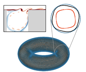
In this work we show that nonlinear correlations can be exploited to identify and enforce this phase coherence in reduced-order models, as shown schematically in figure 1. After projecting data from a direct numerical solution of a quasiperiodic shear-driven cavity flow onto a basis of DMD modes, the recently proposed randomized dependence coefficient (Lopez-Paz, Hennig & Schölkopf Reference Lopez-Paz, Hennig and Schölkopf2013) allows us to clearly distinguish the active degrees of freedom from correlated higher harmonics and nonlinear cross-talk. In this minimal representation, the dynamics occurs on a 2-torus, while the rest of the modes, which arise as triadic interactions of the active variables in the frequency domain, can be expressed as polynomial functions of the dynamically active variables. The restriction to this manifold stabilizes a standard POD-Galerkin model, avoiding both decoherence and energy imbalance. This representation is also a natural basis for data-driven system identification methods; we apply the sparse identification of nonlinear dynamics (SINDy) algorithm (Brunton et al. Reference Brunton, Proctor and Kutz2016) and show that the flow can be accurately described by two independent Stuart-Landau equations.
Schematic of the model reduction approach exploiting nonlinear correlations. The flow fields are first projected onto a linear modal basis  $\boldsymbol {\varPhi }$, yielding modal coefficients $\boldsymbol {\alpha }(t)$. The quasiperiodic dynamics can be described by four degrees of freedom; the rest of the modal coefficients can then be reconstructed with polynomial functions consistent with triadic interactions in the frequency domain. The dynamics of the active degrees of freedom can be modelled either by restricting the POD–Galerkin dynamics to the toroidal manifold or by identifying a simple, interpretable dynamical system with the sparse identification of nonlinear dynamics algorithm.

This laminar, quasiperiodic flow is chosen as an illustrative example where stable and accurate low-dimensional models can be constructed without closure assumptions. In particular, the modal amplitudes can be reconstructed to high accuracy with sparse polynomial regression on the four active degrees of freedom. Although this approach to addressing nonlinear correlations will only be valid for flows with discrete spectral content (i.e. periodic or quasiperiodic dynamics), we expect that the problem of linear modal decompositions overestimating the number of dynamically active degrees of freedom will also be relevant for general advection-dominated flows, motivating future work on nonlinear dimensionality reduction.
This work is organized as follows. In § 2 we use two model partial differential equations (PDEs) to give brief analogies motivating our use of nonlinear correlation. We introduce the open cavity flow and direct numerical simulation in § 3 and give POD and DMD analyses in § 4. Section 5 introduces the reduced-order modelling techniques of Galerkin projection and SINDy. In § 6 we show how nonlinear correlations arise in the modal analysis of the flow and how this can be exploited for the reduced-order models. A comparison and analysis of the various models is given in § 7, followed by a final discussion in § 8.
2. The origins of nonlinear correlation
Many features of projection-based models of advection-dominated flows are demonstrated by simple scalar PDEs. In particular, limitations of the Galerkin representation of hyperbolic problems can be seen in the linear constant-coefficient advection equation, while Burgers’ equation is a minimal example of the key role of nonlinearity in the full Navier–Stokes equations.
2.1. The linear dispersion relation as nonlinear correlation
One of the fundamental reasons that Galerkin models of advection-dominated flows tend to be fragile is that they introduce additional variables that do not correspond to physical degrees of freedom. This is perhaps illustrated most clearly by the linear advection equation on a periodic domain
 \begin{equation} u_t + c u_x = 0, \quad x \in (0, L)\end{equation}
where u is a scalar amplitude, x is the spatial variable, and c is the constant advection speed on a finite domain of length L. For any initial condition  $u(x, 0) = u_0(x)$, this equation has the simple travelling wave solution $u(x, t) = u_0(x - ct)$. Given the initial condition, the only effective degree of freedom is the phase $ct/L$. However, the problem could also be solved by means of a Fourier expansion
 \begin{equation} u(x, t) = \sum_{n={-}\infty}^{\infty} a_n(t) \textrm{e}^{\textrm{i}k_nx} \end{equation}
with  $k_n = 2{\rm \pi} n/L$ with time-varying modal coefficients $a_n(t)$. The Galerkin system in this orthogonal basis (see § 5) is
 \begin{equation} \dot{a}_n(t) ={-}\textrm{i}\omega_n a_n(t), \quad \omega_n = k_n c n = 0, \pm 1, \pm 2, \dots \end{equation}
The relationship between frequency  $\omega$ and wavenumber $k_n$ is the dispersion relation; in this case it implies that all scales are carried at the same speed $c$.
$c$.
With this analytic dispersion relation, (2.3a,b) is equivalent to the travelling wave solution, since  $a_n(t) = \textrm {e}^{-\textrm {i}\omega _n t} a_n(0)$
 \begin{equation} u(x, t) = \sum_{n={-}\infty}^{\infty} a_n(0) \exp({\textrm{i}k_n(x-ct)}) = u_0(x - ct). \end{equation}
However, the Galerkin model has introduced many degrees of freedom in the harmonics  $a_n$ by artificially separating space and time. If the projection is approximated numerically or with empirical basis modes, the estimated system may include some error, so that $\omega _n = k_n c + \epsilon _n$. In this case the Galerkin system will be dispersive, i.e. each wavenumber will propagate with a slightly different speed. The travelling wave solution will tend to lose coherence on a time scale $1/\epsilon$, as shown in figure 2.
Linear advection equation with errors  $\epsilon _n \sim \mathcal {N}(0, \epsilon ^2)$ in the dispersion relation $\omega _n = c k_n$. The Galerkin model (grey) loses coherence with the exact solution (black) over a time scale $1/\epsilon$. If the polynomial correlations implied by the dispersion relation are enforced explicitly, the model is robust to such errors. Nonlinear correlation in the true system, given by (2.5), appears in the Lissajous-type phase portraits of the Fourier coefficients (b–d). Similar behaviour manifests in Galerkin models of nonlinear advection-dominated flows.

An alternative perspective on the dispersion relation is that it specifies nonlinear correlations between the temporal coefficients  $a_n$, removing the spurious degrees of freedom introduced by Galerkin projection. The linear dispersion relation $\omega _n = n k_1 c$ implies the nonlinear relationship for harmonics
 \begin{equation} a_n(t) = \exp({-\textrm{i}n k_1 c t}) a_n(0) \propto a_1^n, \end{equation}
with the proportionality determined by the initial condition. Then the only degree of freedom is  $a_1$, and the travelling wave solution is recovered by the Galerkin model projected onto this mode. In dynamical systems terminology, the solution is restricted to a one-dimensional manifold: a circle representing the phase of the leading Fourier coefficient. In this case the decoherence does not lead to instability because the system is purely linear with purely imaginary eigenvalues, but in nonlinear systems with non-zero linear growth rates the departure from the solution manifold can be catastrophic.
2.2. Triadic interactions and the energy cascade
For more general linear systems the preceding analysis is complicated by non-normality and physical dispersion, and the concept of a dispersion relation is not well defined for nonlinear dynamical systems. Nevertheless, analogous concepts are similarly important in models of nonlinear PDEs. For example, Burgers’ model is a paradigmatic scalar conservation equation illustrating many features of gas dynamics and nonlinear flows more broadly. Burgers’ equation with viscosity  $\epsilon$ is
 \begin{equation} \frac{\partial u}{\partial t} + u \frac{\partial u}{\partial x} = \epsilon \frac{\partial^2u}{\partial x^2}, \quad x \in (0, 2{\rm \pi}). \end{equation}
On a periodic domain, we can apply the same Fourier expansion (2.2) with  $L=2{\rm \pi}$, leading to the Galerkin ordinary differential equation (ODE) system
 \begin{equation} \dot{a}_k ={-}\epsilon k^2 a_k -\textrm{i} k \sum_{\ell={-}\infty}^\infty a_\ell a_{k-\ell}, \quad k = 0, \pm 1, \pm 2, \dots. \end{equation}
 The two right-hand side terms in (2.7), originating from the viscous and nonlinear PDE terms respectively, capture several key features of the full Navier–Stokes equations. First, the convolution-type sum over wavenumbers  $\ell$ includes only pairs that sum to $k$; these are the so-called ‘triadic’-scale interactions. Second, it can be shown that the nonlinear term is energy preserving in the sense that when the energy $a_k a_k^*$ is summed over all wavenumbers the nonlinear term does not contribute to a net change in energy of the system. (A similar result holds for inhomogeneous flows (Schlegel & Noack Reference Schlegel and Noack2015).) This suggests that the only role of nonlinearity is to transfer energy between scales. Meanwhile, the dissipation rate of each mode scales quadratically with wavenumber so that the bulk of dissipation occurs at the smallest scales.
The overall picture of the dynamics in the spectral domain is therefore that the nonlinear term transfers energy from the more energetic large scales to the dissipative small scales. Since (2.7) is very similar to the spectral form of the momentum equations for isotropic turbulence (Tennekes & Lumley Reference Tennekes and Lumley1972), this ‘energy cascade’ is an important feature of real viscous flows as well. The energy cascade points to another often-discussed issue with Galerkin models: if the system is truncated at a wavenumber  $r$ which is not sufficiently large to capture the net dissipation rate, the energy cascade is interrupted and the system of ODEs will overestimate the energy, potentially even becoming unstable.
This issue is fundamentally different from the decoherence discussed in the context of the linear advection equation. For example, the issue of fine-scale dissipation is also present in the heat equation, given by (2.6)–(2.7) without the convective nonlinearity. Whereas the Fourier–Galerkin representation of advection introduces spurious degrees of freedom, this discussion suggests that in the representation of the heat equation all coefficients are dynamically important (self-similarity notwithstanding). The Galerkin system is therefore an ideal representation of the parabolic dynamics of the heat equation, where the fundamental assumption of separation of variables is valid.
The inability of Fourier decomposition and POD to produce efficient representations of travelling wave physics has long been recognized. Fundamentally, these decompositions rely on a space–time separation of variables, which is not a valid assumption for travelling waves. Many extensions to POD have been developed for translationally invariant systems and systems with other symmetries (Rowley & Marsden Reference Rowley and Marsden2000; Reiss et al. Reference Reiss, Schulze, Sesterhenn and Mehrmann2018; Rim, Moe & LeVeque Reference Rim, Moe and LeVeque2018; Mendible et al. Reference Mendible, Brunton, Aravkin, Lowrie and Kutz2020).
For general viscous, nonlinear, advection-driven fluid flows, we might expect advection, triadic interactions and small-scale dissipation to all be relevant as a result of the joint hyperbolic–parabolic structure of the Navier–Stokes equations. The intrinsic dimensionality of the system and, conversely, the inaptitude of the Galerkin model, may not be a priori clear as a result of a complex interplay between these mechanisms.
For example, if the leading degree of freedom  $a_1$ tends to oscillate at a frequency $\omega _0$, representing either a standing or travelling wave, then the $a_2$ dynamics includes a term of the form $a_1^2 \sim \textrm {e}^{2\textrm {i}\omega _0 t}$. Similarly, $\dot {a}_3 \propto a_1 a_2 \sim \textrm {e}^{3\textrm {i}\omega _0 t}$. In the energy cascade picture, these higher-order modes act as forced, damped oscillators and will tend to respond at the forcing frequencies. In this manner, triadic interactions in the wavenumber domain can also give rise to nonlinear correlations in time and triadic structure in the frequency domain.
This effect is not necessarily limited to systems with spatial or temporal periodicity; Rubini et al. (Reference Rubini, Lasagna and Da Ronch2020) investigated the application of system identification methods to a chaotic lid-driven cavity flow and showed that sparse nonlinear coupling, analogous to triadic interactions, were critical for resolving energy transfers across scales of the flow. They distinguish between this empirical, a posteriori sparsity appearing in the statistics and data-driven models, and the structural, a priori sparsity of systems such as (2.7), which is generally lost in Galerkin models of inhomogeneous flows. Similarly, Schmidt (Reference Schmidt2020) recently proposed a bispectral modal analysis technique that leverages approximate sparsity in frequency interactions.
In analogy with the dispersion relation, these processes may result in latent structure not immediately obvious in the Galerkin representation. If this structure is ignored, the behaviour of the model may depart significantly from that of the underlying system. For example, Majda & Timofeyev (Reference Majda and Timofeyev2000) showed that a truncated Galerkin model of the inviscid Burgers equation tends towards equipartition of energy rather than a physical solution as a result of a catastrophic decoherence mechanism. Consequentially, in the following sections we argue that nonlinear correlation and manifold restriction plays an important role in the stability and accuracy of reduced-order models of advection-dominated fluid flows.
3. Flow configuration
The flow considered in the present work is the incompressible shear-driven cavity flow visualized in figure 3. It is a geometrically induced separated boundary layer flow having a number of applications in aeronautics (Yu Reference Yu1977) or for mixing purposes (Chien, Rising & Ottino Reference Chien, Rising and Ottino1986). The leading two-dimensional instability of the flow is localized along the shear layer delimiting the outer boundary layer flow and the inner cavity flow (Sipp & Lebedev Reference Sipp and Lebedev2007; Sipp et al. Reference Sipp, Marquet, Meliga and Barbagallo2010). This oscillatory instability relies essentially on two mechanisms. First, the convectively unstable nature of the shear layer causes perturbations to grow as they travel downstream. Once the perturbations impinge upon the downstream corner of the cavity, instantaneous pressure feedback re-excites the upstream portion of the shear layer. Coupling of these mechanisms gives rise to a linearly unstable feedback loop at sufficiently high Reynolds numbers ( $\textit {Re}_c \gtrsim 4120$, see Sipp & Lebedev Reference Sipp and Lebedev2007). A similar unstable loop exist for compressible shear-driven cavity flows, wherein the instantaneous pressure feedback is replaced by upstream-propagating acoustic waves (Rossiter Reference Rossiter1964; Rowley, Colonius & Basu Reference Rowley, Colonius and Basu2002; Yamouni, Sipp & Jacquin Reference Yamouni, Sipp and Jacquin2013). At higher Reynolds numbers, the slowly recirculating flow inside the cavity can also perturb the shear layer. This inner cavity mode is similar in spatial structure and oscillation frequency to those observed in two-dimensional lid-driven cavity flows (Arbabi & Mezić Reference Arbabi and Mezić2017). Since the shear layer instability and inner-cavity recirculation occur at incommensurate frequencies, the nonlinear coupling between these modes leads to a quasiperiodic dynamics, as illustrated in figure 4.
Computational domain and representative instantaneous vorticity field for the shear-driven cavity flow at  $Re=7500$ highlighting the vortical structures developing along the shear layer.

Fourier spectrum  $\vert \hat {E} ( \omega ) \vert$ of the fluctuation's kinetic energy at $Re=7500$. The high-frequency peak ( $\omega _s \simeq 12)$ corresponds to the shear layer instability while the low-frequency peak ( $\omega _c \simeq 3$) is associated with the inner-cavity dynamics. A few other peaks have been labelled based on the quadratic interactions on the two fundamental frequencies for the sake of illustration. Multiple closely spaced peaks are associated with nearby frequency combinations (e.g. $2 \omega _c \approx \omega _s - 2 \omega _c \approx 6$). Also shown are the real parts of the DMD modes at $\omega _s$ and $\omega _c$.

Despite its apparent simplicity, this strictly two-dimensional linearly unstable flow configuration has served multiple purposes over the past decade: illustration of optimal control and reduced-order modelling (Barbagallo, Sipp & Schmid Reference Barbagallo, Sipp and Schmid2009; Loiseau & Brunton Reference Loiseau and Brunton2018; Leclercq et al. Reference Leclercq, Demourant, Poussot-Vassal and Sipp2019), investigation of the nonlinear saturation process of flow oscillators (Sipp & Lebedev Reference Sipp and Lebedev2007; Meliga Reference Meliga2017) or as an introduction to DMD (Schmid Reference Schmid2010). Recent work has also explored the linear stability of its three-dimensional counterpart, in particular the influence of spanwise endwalls (Liu, Gómez & Theofilis Reference Liu, Gómez and Theofilis2016; Picella et al. Reference Picella, Loiseau, Lusseyran, Robinet, Cherubini and Pastur2018).
The dynamics of the flow is governed by the incompressible Navier–Stokes equations
 \begin{equation} \left.\begin{gathered} \displaystyle \frac{\partial \boldsymbol{u}}{\partial t} + \boldsymbol{\nabla} \boldsymbol{\cdot} \left( \boldsymbol{u} \otimes \boldsymbol{u} \right) ={-} \boldsymbol{\nabla} p + \frac{1}{Re} \nabla^2 \boldsymbol{u} \\ \boldsymbol{\nabla}\boldsymbol{\cdot} \boldsymbol{u} = 0, \end{gathered}\right\} \end{equation}
where  $\boldsymbol {u}(\boldsymbol {x}, t) = (u, v)^\textrm {T}$ is the two-dimensional velocity field and $p$ is the pressure field. The Reynolds number is set to $\textit {Re}=7500$ based on the free-stream velocity $U_{\infty }$ and the depth $L$ of the open cavity. The computational domain and boundary conditions considered herein are the same as in Sipp & Lebedev (Reference Sipp and Lebedev2007), Sipp et al. (Reference Sipp, Marquet, Meliga and Barbagallo2010), Loiseau & Brunton (Reference Loiseau and Brunton2018), Bengana et al. (Reference Bengana, Loiseau, Robinet and Tuckerman2019) and Leclercq et al. (Reference Leclercq, Demourant, Poussot-Vassal and Sipp2019), shown schematically in figure 3.
We perform direct numerical simulation (DNS) of the flow with the Nek5000 spectral element solver (Fischer, Lottes & Kerkemeir Reference Fischer, Lottes and Kerkemeir2008). The mesh consists of 6100 eighth-order spectral elements, equivalent to roughly  $3.8 \times 10^5$ grid points, refined towards the walls and shear layer. The domain is therefore somewhat over-resolved compared with similar studies in order to minimize any numerical errors in the Galerkin projection for higher-order modes. Diffusive terms are integrated with third-order backwards differentiation, while convective terms are advanced with a third order extrapolation. We retain 30 000 snapshots from the DNS at sampling rate $\Delta t = 10^{-2}$, a frequency roughly fifty times larger than the high-frequency oscillation of the shear layer.
Figure 3 depicts an instantaneous vorticity field obtained from DNS once the flow has reached a statistical steady state. It shows the advection of a vortical structure along the shear layer before it impinges the downstream corner of the cavity. These shear layer oscillations arise as a linear instability mode of the steady base flow above  $\textit {Re}_c \gtrsim 4120$ (Sipp & Lebedev Reference Sipp and Lebedev2007). However, the Reynolds number of the present flow ( $\textit {Re}=7500$) is significantly larger than this critical Reynolds number, so the typical amplitude of fluctuations is not infinitesimal and the associated Reynolds stressed are not negligible.
The physics of this flow are therefore fundamentally nonlinear in at least two respects. First, the growth of the instability modes is checked by the Stuart–Landau nonlinear stability mechanism, in which finite Reynolds stresses deform the steady base flow into the post-transient mean (Sipp & Lebedev Reference Sipp and Lebedev2007; Meliga Reference Meliga2017). Second, a stability analysis of the time-averaged mean flow at this Reynolds number reveals a second, weaker instability associated with lower-frequency oscillations inside the cavity; see Appendix A and Sipp et al. (Reference Sipp, Marquet, Meliga and Barbagallo2010). The incommensurate frequencies of these two instabilities give rise to a quasiperiodic oscillatory dynamics.
Because the unstable base flow is of limited relevance in the statistically stationary regime, it is more natural to decompose the instantaneous velocity field into a time-averaged mean flow  $\bar {\boldsymbol {u}}(\boldsymbol {x})$ and zero-mean fluctuations $\boldsymbol {u}^{\prime }(\boldsymbol {x}, t)$. For a detailed analysis of the choice between base- and mean-flow expansions, see Sipp & Lebedev (Reference Sipp and Lebedev2007).
Figure 4 shows the Fourier spectrum of the kinetic energy of the fluctuating component
 \begin{equation} E(t) = \displaystyle \tfrac{1}{2} \int_{\varOmega} \boldsymbol{u}^{\prime}(\boldsymbol{x}, t) \boldsymbol{\cdot} \boldsymbol{u}^{\prime}(\boldsymbol{x}, t) \, \mathrm{d}\varOmega \end{equation}
integrated over the domain  $\varOmega$. Such a spectrum is characteristic a of quasiperiodic dynamics, as recently observed for a similar flow by Leclercq et al. (Reference Leclercq, Demourant, Poussot-Vassal and Sipp2019). As demonstrated below, the two main frequencies correspond either to the dynamics of the vortical structures along the shear layer ( $\omega _s$) or to the low-frequency unsteadiness taking place within the cavity ( $\omega _c$). The power spectrum consists of approximately discrete peaks, each of which can be accounted for by the sum or difference of these fundamental frequencies and their harmonics. The observation that this spectrum can be generated using only two main frequencies lets us hypothesize that the dynamics of the fluctuation $\boldsymbol {u}^{\prime }(\boldsymbol {x}, t)$ around the mean flow $\bar {\boldsymbol {u}}(\boldsymbol {x})$ is amenable to a low-dimensional representation. This flow is therefore of intermediate complexity, between weakly nonlinear flows, which can be accurately described with normal form dynamics, and fully turbulent flows, which have many dynamical degrees of freedom and would likely require careful closure modelling to approximately model the evolution of large-scale coherent structures.
4. Modal analysis
Linear modal analysis is a powerful tool for extracting low-dimensional coherent structure in flows, even those characterized by strong nonlinearity. Here, we give only a brief description; see Taira et al. (Reference Taira, Brunton, Dawson, Rowley, Colonius, McKeon, Schmidt, Gordeyev, Theofilis and Ukeiley2017) for a comprehensive survey. We focus on truncated (rank  $r$) affine decompositions with space–time separation, of the form
 \begin{equation} \boldsymbol{u}(\boldsymbol{x}, t) \simeq \bar{\boldsymbol{u}}(\boldsymbol{x}) + \sum_{k=1}^r \boldsymbol{\psi}_k(\boldsymbol{x}) a_k(t), \end{equation}
including for example global stability analysis (Theofilis Reference Theofilis2011), POD (Lumley Reference Lumley1967; Holmes et al. Reference Holmes, Lumley and Berkooz1996) and DMD (Schmid Reference Schmid2010; Rowley et al. Reference Rowley, Mezić, Bagheri and Schlatter2009b), but excluding approaches such as non-modal stability analysis (Schmid Reference Schmid2007; McKeon & Sharma Reference McKeon and Sharma2010) and spectral POD (Towne, Schmidt & Colonius Reference Towne, Schmidt and Colonius2018). Broadly speaking, the goal of modal analysis is to identify a suitable basis  $\{\boldsymbol {\psi }_k \}_{k=1}^r$ in which to represent the flow kinematics, while the reduced-order dynamical systems models discussed in § 5 treat the time evolution of the coefficients $\boldsymbol {a}(t)$. Since the state is specified by the $r$-dimensional coefficient vector, (4.1) is a linear dimensionality reduction.
4.1. Proper orthogonal decomposition
One of the most widely used techniques for dimensionality reduction and modal analysis is POD, which solves the optimization problem
 \begin{equation} \textrm{minimize}~_{\{ \boldsymbol{\psi}_k \} } \left \langle \left\|{ \boldsymbol{u}' - \sum_{k=1}^r \boldsymbol{\psi}_k \left( \boldsymbol{u}' , \boldsymbol{\psi}_k \right)_{\varOmega}} \right\|^2 \right \rangle \quad \textrm{subject to}~ \left( \boldsymbol{\psi}_j, \boldsymbol{\psi}_k \right)_{\varOmega} = \delta_{jk} \end{equation}
in the norm induced by the energy inner product
 \begin{equation} \left( \boldsymbol{u}, \boldsymbol{v} \right)_{\varOmega} \equiv \int_\varOmega \boldsymbol{u}(\boldsymbol{x}) \boldsymbol{\cdot} \boldsymbol{v}^*(\boldsymbol{x}) \, {\text d} \varOmega, \end{equation}
where  $\langle \cdot \rangle$ is an ensemble average, approximated in practice by a time average, $\delta _{jk}$ is the Kronecker delta and the star indicates a complex conjugate. For data on a non-uniform mesh, the inner product is computed with a weighted Riemann sum, approximating ${\text d} \varOmega$ with the mass matrix of the discretization. Thus, the objective is to minimize the residual energy in a linear subspace of $r$ orthonormal modes, providing an optimal low-rank representation of the flow.
This problem can be solved with the calculus of variations, leading to the result that the modes  $\{ \boldsymbol {\psi }_k \}$ are eigenfunctions of the correlation tensor $\mathcal {\boldsymbol C}(\boldsymbol {x}, \boldsymbol {x}')$:
 \begin{equation} \int_\varOmega \mathcal{\boldsymbol C}(\boldsymbol{x}, \boldsymbol{x}') \boldsymbol{\psi}_k(\boldsymbol{x}') \, {\text d} \varOmega' = \sigma_k^2 \boldsymbol{\psi}_k(\boldsymbol{x}), \end{equation}
where  $\mathcal {\boldsymbol C}(\boldsymbol {x}, \boldsymbol {x}') = \langle \boldsymbol {u}(\boldsymbol {x}, t) \boldsymbol {u}^*(\boldsymbol {x}', t) \rangle$ and $\{ \sigma _k \}$ are the POD eigenvalues, representing the average fluctuation kinetic energy captured by each mode. The coefficients $\boldsymbol {a}(t)$ can be extracted with the projection $a_k = \left ( \boldsymbol {u}', \boldsymbol {\psi }_k \right )_{\varOmega }$. In practice the correlation tensor is often not feasible to construct, since it scales with the square of the discretized state dimension. Instead it is approximated numerically with either a singular value decomposition (SVD) or the snapshot method (Sirovich Reference Sirovich1987; Holmes et al. Reference Holmes, Lumley and Berkooz1996; Taira et al. Reference Taira, Brunton, Dawson, Rowley, Colonius, McKeon, Schmidt, Gordeyev, Theofilis and Ukeiley2017). In this work we use the snapshot method as implemented in the modred library (Belson, Tu & Rowley Reference Belson, Tu and Rowley2014), since it does not require storing the entire time series of high-dimensional discretized velocity fields in memory.
The method of snapshots is based on simple linear algebraic manipulations of the discretized form of the eigenvalue problem (4.4). We omit a derivation here as it is given in standard references, e.g. Holmes et al. (Reference Holmes, Lumley and Berkooz1996). Rather than form the spatial correlation tensor  $\mathcal {\boldsymbol C}(\boldsymbol {x}, \boldsymbol {x}')$, we compute a temporal correlation matrix $\boldsymbol{\mathsf{R}}$ with entries defined by
 \begin{equation} R_{jk} = \frac{1}{M} \left( \boldsymbol{u}(t_j), \boldsymbol{u}(t_k) \right)_{\varOmega}, \quad j, k = 1, 2, \dots, M. \end{equation}
The temporal correlation matrix  $\boldsymbol{\mathsf{R}}$ has dimensions $M \times M$, and is typically much smaller than the discretized spatial correlation tensor. The eigenvalues of $\boldsymbol{\mathsf{R}}$ approximate those of $\mathcal {\boldsymbol C}$, and the modes that solve the discretized form of (4.4) are also given by
 \begin{equation} \boldsymbol{\psi}_k = \frac{1}{\sigma_k \sqrt{M}} \sum_{j=1}^M \boldsymbol{u}(t_j) W_{jk}, \end{equation}
where  $\boldsymbol{\mathsf{R}}\boldsymbol{\mathsf{W}} = \boldsymbol{\mathsf{W}} \boldsymbol {\varSigma }^2$ is the eigendecomposition of $\boldsymbol{\mathsf{R}}$.
The POD has the following useful properties:
(i) The spatial modes form an orthonormal set: $\left ( \boldsymbol {\psi }_j, \boldsymbol {\psi }_k \right )_{\varOmega } = \delta _{jk}$.
(ii) The temporal coefficients are linearly uncorrelated:
$\langle a_j a_k \rangle = \sigma _k^2 \delta _{jk}$.(iii) The modes can be ranked hierarchically by average energy content
$\sigma _k^2$.


Since POD can be viewed as a continuous form of the SVD, these properties are analogous to unitarity of the matrices of left and right singular vectors. The singular values quantify the statistical variance captured by the low-rank SVD approximation. As a consequence of the hierarchical ordering, the POD can be computed without a priori specification of the rank  $r$, with the truncation determined later by a threshold based on the residual energy. Finally, since the modes are a linear combination of DNS snapshots, the reconstruction (4.1) automatically satisfies the incompressibility constraint and boundary conditions.
We compute the POD from 4000 fields sampled at  $\Delta t = 0.05$, approximately ten times the shear layer frequency, using the method of snapshots (Sirovich Reference Sirovich1987). This is around 13 % of the total number of fields retained from the DNS, but is sufficient for statistical convergence of the leading modes. The singular value spectrum and residual energy are shown in figure 5. The singular values converge relatively quickly; the first pair of modes contain 70 % of the fluctuation kinetic energy, the first six account for ${\sim }90\,\%$, and by $r=64$ approximately $99.97\,\%$ of the energy is recovered. We retain 64 modes for further analysis and note that our modelling results are insensitive to moderate changes in truncation.
Singular value spectrum of the quasiperiodic cavity flow. Black dots represent the normalized squared singular values of the snapshot correlation matrix, indicating the fraction of fluctuation kinetic energy resolved by each mode. Red crosses indicate the fraction of residual energy, or normalized cumulative sum of squared singular values. Dashed lines indicate the number of modes retained ( $r=64$).

Still, as we will show in § 6, the intrinsic dimensionality of the system is much smaller than that of the linear subspace required for reconstruction. As with the advection system in § 2, this is partly due to the representation of travelling waves, as shown in figure 6. This is made clearer by a DMD analysis.
Harmonic modes identified from POD and DMD analysis. The spatial fields and phase portraits both indicate that certain mode pairs are harmonics arising from the description of wavelike motion in the shear layer and inner cavity. Because DMD is based on both spatial and temporal correlation, this structure is especially pronounced in the DMD coefficients. The vorticity plots are real parts of the DMD modes, but analogous modes exist in the POD basis.

4.2. Dynamic mode decomposition
Although POD is guaranteed to provide an energy-optimal spatial reconstruction of the flow field, it sacrifices all temporal information in the computation of the correlation tensor. The POD basis is therefore purely kinematic and contains no dynamic information. An alternative approach is to compute the discrete Fourier transform of the fields, which suffers from the opposite issue: frequency information is perfectly resolved, but the result is not necessarily associated with a useful reduced-order linear subspace for kinematic representation. DMD, introduced by Schmid (Reference Schmid2010), is a useful compromise between these extremes.
DMD seeks to approximate a discrete-time linear evolution operator defined by
 \begin{equation} \textrm{minimize}~_{\mathcal{\boldsymbol A}} \left \langle \| \boldsymbol{u}(\boldsymbol{x}, t_{n+1}) - \mathcal{\boldsymbol A} \boldsymbol{u}(\boldsymbol{x}, t_{n}) \|^2 \right \rangle. \end{equation}
The description of nonlinear dynamics in terms a linear evolution operator acting on observables has a deep connection to Koopman theory (Rowley et al. Reference Rowley, Mezić, Bagheri and Schlatter2009b; Mezić Reference Mezić2013; Brunton et al. Reference Brunton, Budišić, Kaiser and Kutz2022). We will discuss this in § 8, but in terms of modal analysis it is more useful to think of DMD as solving an alternative optimization to (4.2).
Given a series of snapshots, a least-squares solution to (4.7) could be found in terms of the pseudoinverse of the snapshot matrix. However, this calculation is typically computationally prohibitive, ill conditioned and disregards low-dimensional structure in the flow. Instead, DMD seeks to approximate the spectral properties of the operator  $\mathcal {\boldsymbol A}$ without explicitly forming it. There are a variety of algorithms to compute DMD in conditions with limited or noisy data, but beginning with high-fidelity DNS snapshots we follow the simple exact DMD algorithm introduced by Tu et al. (Reference Tu, Rowley, Luchtenburg, Brunton and Kutz2014).
Beginning with a truncated POD basis and associated coefficients  $\{\boldsymbol {a}(t_n) \}_{n=1}^M$, the coefficients are arranged into time-shifted matrices $\boldsymbol{\mathsf{X}} = \left [\boldsymbol {a}(t_1) \enspace \boldsymbol {a}(t_2)\enspace \cdots \enspace \boldsymbol {a}(t_M-1)\right ]$ and $\boldsymbol{\mathsf{X}}^\prime = \left [\boldsymbol {a}(t_2) \enspace \boldsymbol {a}(t_3)\enspace \cdots \enspace \boldsymbol {a}(t_M) \right ]$. Here, we assume the $\{t_n\}$ are evenly sampled in time, but it is possible to account for situations where this is not the case. A least-squares solution to (4.7) in the POD subspace is $\tilde {\boldsymbol{\mathsf{A}}} = \boldsymbol{\mathsf{X}}^\prime \boldsymbol{\mathsf{X}}^+$, where $\boldsymbol{\mathsf{X}}^+$ is the pseudoinverse. With some assumptions, the spectrum of $\mathcal {\boldsymbol A}$ is approximated by the spectrum of $\tilde {\boldsymbol{\mathsf{A}}}$, which can now be easily computed via an eigendecomposition
 \begin{equation} \tilde{\boldsymbol{\mathsf{A}}} = \boldsymbol{\mathsf{V}} \boldsymbol{\varLambda} \boldsymbol{\mathsf{V}}^{{-}1}, \end{equation}
with  $\tilde {\boldsymbol{\mathsf{A}}}, \boldsymbol{\mathsf{V}}, \boldsymbol {\varLambda } \in \mathbb {C}^{r \times r}$. For details on theory and algorithms of DMD, see Tu et al. (Reference Tu, Rowley, Luchtenburg, Brunton and Kutz2014) and Kutz et al. (Reference Kutz, Brunton, Brunton and Proctor2016). Based on this eigendecomposition, complex-valued DMD modes $\{ \boldsymbol {\phi }_k(\boldsymbol {x}) \}$ and associated projection coefficients $\boldsymbol {\alpha }(t)$ are linear combinations of the POD modes and coefficients, given by
 \begin{equation} \boldsymbol{\phi}_k(\boldsymbol{x}) = \sum_{j=1}^r \boldsymbol{\psi}_j(\boldsymbol{x}) V_{jk} \quad \boldsymbol{\alpha}(t) = \boldsymbol{\mathsf{V}}^{{-}1} \boldsymbol{a}(t). \end{equation}
In principle the approximate time evolution is specified by the DMD eigenvalues  $\{\lambda _k\} = \mathrm {diag}(\boldsymbol {\varLambda })$, but in terms of reduced-order modelling the decomposition can also be viewed as an alternative expansion to (4.1)
 \begin{equation} \boldsymbol{u}(\boldsymbol{x}, t) \simeq \bar{\boldsymbol{u}}(\boldsymbol{x}) + \sum_{k=1}^r \boldsymbol{\phi}_k (\boldsymbol{x}) \alpha_k(t). \end{equation}
The DMD coefficient vector  $\boldsymbol {\alpha }(t)$ may then be modelled as a time series, as with the POD coefficients $\boldsymbol {a}(t)$.
This representation is essentially a similarity transformation of the POD basis; the two encode the same information and span the same subspace. However, the time dependence in the optimization problem leads DMD to transform the POD basis to modes that tend to have similar frequency content. In terms of the present analysis, figure 6 illustrates the practical relevance of this. Whereas POD happens to identify modes that are roughly coherent in time by coincidence only, the DMD modes are closer to pure harmonics. This perspective on DMD also explains the approximately discrete peaks in figure 4; each DMD eigenvalue (shown in figure 7) can be identified with some combination of the fundamental frequencies of modes  $k=1$ and $k=5$.
DMD frequencies  $\omega _k$ and average energy $E_k = \langle |\alpha _k|^2 \rangle$ along with vorticity plots for the real part of the most energetic modes. The second mode pair ( $k=3, 4$) is a harmonic of the leading pair ( $k=1,2$), while the third pair ( $k=5, 6$) represents the low-frequency inner-cavity motion. Other modes (e.g. $k=7, 8$) are either harmonics or indicate nonlinear frequency cross-talk between these leading modes, as in figure 4.

Based on the results in §§ 6 and 7, we hypothesize that DMD also filters frequency content and accentuates nonlinear correlations for modes that are not pure harmonics. This approximate nonlinear algebraic dependence clearly indicates a manifold structure of much lower dimensionality than the linear subspace. Given these implications, the results presented below are based on the DMD expansion (4.10).
5. Reduced-order models
The modal analyses discussed in § 4 may be viewed as linear dimensionality reduction methods that transform the system to a compact coordinate system in which low-dimensional dynamical systems models can be developed. In addition to an inexpensive surrogate for the flow, such models can provide valuable insight into latent structure of the physical solutions. Broadly speaking, two of the most common approaches to nonlinear reduced-order modelling are projection-based models and data-driven system identification, though many more tools are available for linear model reduction; see for instance Antoulas (Reference Antoulas2005) and Benner, Gugercin & Willcox (Reference Benner, Gugercin and Willcox2015). In this section we give a brief overview of relevant material on projection-based modelling (§ 5.1) and the SINDy framework for system identification (§ 5.2).
5.1. POD–Galerkin modelling
In projection-based modelling, the discretized governing equations are projected onto an appropriate modal basis. For simple geometries, this might be done analytically, as for the periodic problems in § 2 and in Noack & Eckelmann (Reference Noack and Eckelmann1994), for instance. Although general and expressive, this approach becomes challenging on complex domains and does not take advantage of structure in the solutions to the particular PDE. As a result, it is increasingly common to project onto an empirical basis, such as POD modes. Assuming that the flow is statistically stationary and the ensemble is sufficiently resolved, this provides optimal kinematic resolution in an orthonormal basis. The following Galerkin projection procedure then leads to a minimum-residual system of ODEs in this basis.
Let  $\mathcal {\boldsymbol N}[\boldsymbol {u}] = 0$ be the Navier–Stokes equations in implicit form. By approximating the flow field with a truncated linear combination of basis functions as in (4.1), we expect some residual error $\boldsymbol {r}(x, t)$ in the approximated dynamics defined by
 \begin{equation} \boldsymbol{r}(\boldsymbol{x}, t) = \mathcal{\boldsymbol N}\left[ \bar{\boldsymbol{u}}(\boldsymbol{x}) + \sum_{\ell = 1}^r \boldsymbol{\psi}_\ell(\boldsymbol{x}) a_\ell(t) \right]. \end{equation}
In order to minimize the residual in this basis, the Galerkin projection condition is that that the residual be orthogonal to each mode
 \begin{equation} 0 = \left( \boldsymbol{r}, \boldsymbol{\psi}_k \right)_{\varOmega} = \left( \mathcal{\boldsymbol N}\left[ \bar{\boldsymbol{u}}(\boldsymbol{x}) + \sum_{\ell = 1}^r \boldsymbol{\psi}_\ell(\boldsymbol{x}) a_\ell(t) \right], \boldsymbol{\psi}_k \right)_{\varOmega}. \end{equation}
This leads to the linear-quadratic system of ODEs (Holmes et al. Reference Holmes, Lumley and Berkooz1996; Noack et al. Reference Noack, Morzynski and Tadmor2011)
 \begin{equation} \dot{a}_k = C_k + \sum_{\ell = 1}^r L_{k \ell} a_\ell + \sum_{\ell = 1}^r \sum_{m = 1}^r Q_{k \ell m} a_\ell a_m, \end{equation}
with constant, linear and quadratic terms given by
 \begin{gather} C_k = \left( -\boldsymbol{\nabla} \boldsymbol{\cdot} (\bar{\boldsymbol{u}} \otimes \bar{\boldsymbol{u}} ) + \frac{1}{\textit{Re}} \nabla^2 \bar{\boldsymbol{u}} , \boldsymbol{\psi}_k \right)_{\varOmega} \end{gather}
 \begin{gather}L_{k \ell} = \left( -\boldsymbol{\nabla} \boldsymbol{\cdot} (\bar{\boldsymbol{u}} \otimes \boldsymbol{\psi}_\ell + \boldsymbol{\psi}_\ell \otimes \bar{\boldsymbol{u} } ) + \frac{1}{\textit{Re}} \nabla^2 \boldsymbol{\psi}_\ell , \boldsymbol{\psi}_k \right)_{\varOmega} \end{gather}
 \begin{gather}Q_{k \ell m} = \left( -\boldsymbol{\nabla}\boldsymbol{\cdot} (\boldsymbol{\psi}_m \otimes \boldsymbol{\psi}_\ell + \boldsymbol{\psi}_\ell \otimes \boldsymbol{\psi}_m ) , \boldsymbol{\psi}_k \right)_{\varOmega}. \end{gather}
Note that the constant term vanishes if the flow is expanded about a steady-state solution of the governing equations. Since the mean flow in this case is not a solution, this term represents important mean-flow forcing and is not negligible. Here, we have also neglected the pressure term, though including it does not significantly change any of the results; for detailed discussion of this point see Noack, Papas & Monkewtiz (Reference Noack, Papas and Monkewtiz2005).
In principle, we might expect that the POD–Galerkin system (5.3) leads to approximate solutions with comparable accuracy to the resolution of the expansion basis. However, for reasons introduced in § 2, the long-time behaviour of the reduced-order model may deviate significantly from that of the underlying physical system. In particular, solutions of the model are not constrained to lie on an invariant manifold of the flow. For instance, coefficients associated with shear layer or inner-cavity harmonics evolve independently from the fundamental modes, eventually leading to an unphysical loss of coherence. This effect cannot necessarily be attributed to any particular mode or interaction term, but is related to the structure of the model itself when the POD–Galerkin method is applied to advection-dominated flows.
Figure 8 shows the evolution of the fluctuation kinetic energy as predicted by the POD–Galerkin system for various levels of truncation  $r$. Although the estimate does tend to improve with increasing $r$, none of these models capture the quasiperiodic dynamics of the flow, and most exhibit significant instability. This is true despite (and, we will argue, because of) the fact that these models have many more kinematic degrees of freedom than the true dynamics underlying the post-transient cavity flow.
Evolution of the fluctuation kinetic energy predicted by POD–Galerkin reduced-order models of various dimensions along with DNS values. Though all values of  $r$ shown here capture sufficient dissipation to remain at finite energy, none resolves the true quasiperiodic dynamics.

Finally, a model similar to (5.3) may also be derived beginning with the DMD expansion (4.10). In this case, since the DMD basis is not orthonormal, the Galerkin projection must be replaced with the more general oblique projection of Petrov–Galerkin methods (Benner et al. Reference Benner, Gugercin and Willcox2015). We implement this with a coordinate transform of the standard POD–Galerkin model based on the DMD eigenvector matrix  $\boldsymbol{\mathsf{V}}$, i.e. $\boldsymbol {a} = \boldsymbol{\mathsf{V}} \boldsymbol {\alpha }$. For instance, a DMD–Petrov–Galerkin model with the same truncation as the original POD model has dynamics
 \begin{equation} \dot{\alpha}_k = \tilde{C}_k + \sum_{\ell = 1}^r \tilde{L}_{k \ell} a_\ell + \sum_{\ell = 1}^r \sum_{m = 1}^r \tilde{Q}_{k \ell m} a_\ell a_m, \end{equation}
with the modified constant, linear and quadratic terms given in tensor summation notation by
 \begin{gather} \tilde{C}_k = V^{{-}1}_{k \mu} C_\mu \end{gather}
 \begin{gather}\tilde{L}_{k \ell} = V^{{-}1}_{k \mu} L_{\mu \nu} V_{\nu \ell} \end{gather}
 \begin{gather}\tilde{Q}_{k \ell m} = V^{{-}1}_{k \mu} Q_{\mu \nu \rho} V_{\nu \ell} V_{\rho m}. \end{gather}
The DMD–Petrov–Galerkin model can also be truncated differently from the POD–Galerkin model by selecting a subset of the DMD eigenvectors, so that  $\boldsymbol {a} = \tilde {\boldsymbol{\mathsf{V}}} \boldsymbol {\alpha }$ with $\boldsymbol {a} \in \mathbb {R}^r$, $\boldsymbol {\alpha } \in \mathbb {C}^s$ and $\tilde {\boldsymbol{\mathsf{V}}} \in \mathbb {C}^{r \times s}$, and with $\boldsymbol{\mathsf{V}}^{-1}$ replaced by the pseudoinverse $\tilde {\boldsymbol{\mathsf{V}}}^+$ in (5.6).
Since this transformation is a rotation in the space of modal coefficients, the dynamics and qualitative behaviour of the DMD–Galerkin models do not change compared with figure 8. However, in the following we exploit nonlinear correlations in the coefficients to restrict the dynamics to the manifold of the flow; this is more convenient in the near-harmonic DMD basis, shown in figure 6. Since DMD analysis seeks to approximate the spectrum associated with a linear evolution operator of the flow, this might be considered analogous to the diagonalization step of a centre manifold or normal form analysis.
5.2. Sparse identification of nonlinear dynamics
As an alternative to projection-based reduced-order modelling, a low-dimensional system can be approximated directly from the data in a procedure typically called system identification. In a continuous-time setting, this is done by estimating parameters  $\boldsymbol {\varXi }$ for a function $\boldsymbol {f}(\boldsymbol {a}; \boldsymbol {\varXi }) \approx \dot {\boldsymbol {a}}$ that solve the approximation problem
 \begin{equation} \textrm{minimize}~_{\boldsymbol{\varXi}} \left \langle \| \dot{\boldsymbol{a}} - \boldsymbol{f}(\boldsymbol{a}; \boldsymbol{\varXi}) \|^2 \right \rangle. \end{equation}
This is similar to the residual minimization in Galerkin projection, except that knowledge of the governing equations is neither required nor assumed. Instead, some intuition about the structure of the dynamics is typically encoded in the parameterization of  $\boldsymbol {f}$. Different parameterizations lead to symbolic regression (Schmidt & Lipson Reference Schmidt and Lipson2009), operator inference (Peherstorfer & Willcox Reference Peherstorfer and Willcox2016) or deep learning (Vlachas et al. Reference Vlachas, Byeon, Wan, Sapsis and Komoutsakos2018). In the discrete-time counterpart to (5.7), the nonlinear autoregressive moving average model with exogenous inputs (NARMAX) framework provides a powerful approach that can incorporate time delays, stochastic forcing and exogenous inputs (Billings Reference Billings2013).
In this work we apply the SINDy approach to system identification (Brunton et al. Reference Brunton, Proctor and Kutz2016). Let  $\boldsymbol {\varTheta }(\boldsymbol {a})$ denote a library of candidate functions of the time series $\boldsymbol {a}(t)$, e.g.
 \begin{equation} \boldsymbol{\varTheta}\left(\left[a_1 \quad a_2 \right]^\textrm{T} \right) = \left[a_1 \quad a_2 \quad a_1^2 \quad a_1 a_2 \quad a_2^2 \quad \cdots \right]^\textrm{T}. \end{equation}
We seek a sparse approximation  $\dot {\boldsymbol {a}}\approx \boldsymbol {f}(\boldsymbol {a}; \boldsymbol {\varXi }) = \boldsymbol {\varXi } \boldsymbol {\varTheta }(\boldsymbol {a})$ in the range of these candidate functions. We can frame this as a linear algebra problem by forming the $r \times M$ data matrix $\boldsymbol{\mathsf{X}}$ as in § 4.2, where each column is a snapshot of modal coefficients in time. Similarly, we estimate the time derivative $\dot {\boldsymbol{\mathsf{X}}}$, in this case with second-order central differences. The SINDy formulation of the optimization problem (5.7) is then
 \begin{equation} \textrm{minimize}~_{\boldsymbol{\varXi}} \left\|{\dot{\boldsymbol{\mathsf{X}}} - \boldsymbol{\varXi} \boldsymbol{\varTheta}(\boldsymbol{\mathsf{X}}) }\right\|_2^2 + \gamma \|{\boldsymbol{\varXi}}\|_0, \end{equation}
where  $\|{\cdot }\|_p$ indicates the $p$-norm and $\gamma$ is some regularization weight. This optimization problem is non-convex and requires a combinatorial search over function combinations. To avoid this, we follow Loiseau (Reference Loiseau2020) and approximate the solution to (5.9) with the greedy forward regression orthogonal least squares (FROLS) algorithm used in NARMAX analysis (Billings Reference Billings2013). See Brunton et al. (Reference Brunton, Proctor and Kutz2016), Loiseau & Brunton (Reference Loiseau and Brunton2018) and Loiseau (Reference Loiseau2020) for details on SINDy reduced-order modelling of fluid flows.
Although the systems obtained from POD–Galerkin projection will be dense in general, we expect that the dynamics can be closely approximated by a sparse combination of candidate functions. This may be justified intuitively by the sparse structure of the triadic interactions in isotropic flow (see § 2.2), where only  $r^2$ out of $r^3$ possible interactions are admissible. Moreover, as observed in § 4.2, DMD approximates a diagonalization of the evolution operator, so that by analogy with normal form theory we may reasonably hope for a minimal representation of the dynamics if we work with DMD coefficients $\boldsymbol {\alpha }$ rather than POD coefficients $\boldsymbol {a}$. More generally, sparsity promotion reflects the inductive bias of Occam's razor or Pareto analysis, where we expect that the most important features of the dynamics will be due to a small subset of terms.
For incompressible flows, it has been repeatedly demonstrated that a library of low-order polynomials provides a good basis of functions. Quadratic terms are clearly necessary to capture the advective nonlinearity of the Navier–Stokes equations, but cubic terms allow the model to resolve Stuart–Landau-type nonlinear stability mechanisms (Loiseau & Brunton Reference Loiseau and Brunton2018). From a dynamical systems perspective, higher-order terms may be necessary to describe phenomena such as subcritical bifurcations, but are not necessary to resolve the nonlinear oscillator behaviour in the present case.
For PDEs with more general nonlinearity, low-order polynomials still present an attractive basis for SINDy. In many interesting regimes the effect of the nonlinearity may be relatively weak, so that quadratic and cubic polynomials can be seen as second- or third-order Taylor series approximations to the underlying nonlinearity. Moreover, even strongly nonlinear systems can be lifted with a change of variables to a coordinate system wherein the dynamics is linear quadratic (Rowley, Colonius & Murray Reference Rowley, Colonius and Murray2004; Qian et al. Reference Qian, Kramer, Peherstorfer and Willcox2020).
6. Nonlinear correlations
Sections 4 and 5 recapitulate well-known methodology for analysing and modelling unsteady fluid flows. With a modal expansion and model reduction, the formally infinite-dimensional PDE can be reduced to a set of coupled, nonlinear ODEs mimicking the structure of the physical system. However, the POD analysis indicates that dozens of modes are necessary for an approximately complete kinematic representation in a linear basis, while the DMD analysis and power spectrum suggest that the dynamics of the flow is quasiperiodic. A minimal description of the post-transient flow should therefore require only a pair of oscillators evolving on a 2-torus, comprising four degrees of freedom.
This discrepancy can be understood qualitatively in light of the discussion in § 2. Advection of nearly periodic fluctuations leads to the appearance of harmonic modes, as shown in figures 6 and 7. Similarly, cross-talk between the incommensurate dominant frequencies gives rise to modes that are not pure harmonics of either frequency. In the low-dimensional subspace spanned by the leading POD/DMD modes, these can be viewed as triadic interactions in the frequency domain. Again, since we seek structure that is coherent at distinct frequencies, we will focus on the DMD coefficients in the following.
6.1. A model quasiperiodic cascade
Consider a model system of ODEs including cascading triadic-type interactions of the form of (2.7) where self-sustaining oscillations drive higher-order degrees of freedom
 \begin{gather} a_1 = A \textrm{e}^{\textrm{i} \omega_a t}, \quad b_1 = B \textrm{e}^{\textrm{i} \omega_b t} , \end{gather}
 \begin{gather}\dot{a}_k = \sum_{|\ell| < k} a_{\ell}a_{k - \ell}, \quad \dot{b}_k = \sum_{|\ell| < k} b_{\ell}b_{k - \ell}, \quad \dot{c}_k = \sum_{|\ell| < k} a_{\ell}b_{k - \ell}, \quad k > 1. \end{gather}
For  $k=2$ the only interactions are at $|\ell | = 1$, generating second harmonics for $a_2$ and $b_2$, and oscillations at $\omega _a + \omega _b$ for $c_2$. At $k=3$, the forcing includes the $k=2$ terms, generating third harmonics for $a_3$ and $b_3$ and cross-talk for $c_3$. Up to some complex scaling the solutions take the form
 \begin{gather} a_2 = A^2 \exp({2\textrm{i}\omega_a t}), \quad b_2 = B^2 \exp({2\textrm{i}\omega_b t}), \quad c_2 = A B \exp({\textrm{i}(\omega_a + \omega_b) t}), \end{gather}
 \begin{gather} \left.\begin{gathered} a_3 = A^3 \exp({3\textrm{i}\omega_a t}), \quad b_3 = B^3 \exp({3\textrm{i}\omega_b t}), \\ c_3 = AB^2 \exp({\textrm{i}(\omega_a + 2 \omega_b) t}) + A^2B \exp({\textrm{i}(2\omega_a + \omega_b) t}). \end{gathered}\right\} \end{gather}
By  $k=3$ the response of the $c_k$ cross-talk variable does not represent pure frequency content. If these represented modal coefficients we would expect the dynamics at (for instance) $\omega _a + 2\omega _b$ and $2\omega _a + \omega _b$ corresponds to different spatial structures so $c_3$ and higher-order terms would be separated into distinct coefficients. This serves to emphasize that the temporal coefficients and low-dimensional ODEs are only convenient representations of the full spatio-temporal dynamics and are not fundamental physical quantities.
A global observable such as the energy analogue  $\sum _k (|a_k|^2 + |b_k|^2 + |c_k|^2)$ will have frequency content at all integer combinations of $\omega _a$ and $\omega _b$. As with the linear advection equation in § 2.1, these higher-order coefficients can be expressed as algebraic functions of the fundamental oscillators. For instance, the cross-talk variable $c_3$ can be replaced by $a_1 b_1^2 + a_1^2 b_1$, up to scaling. This example shows that periodic oscillation with cascading triadic interactions can generate quasiperiodic time series, point spectra similar to figure 4 and nonlinear algebraic dependence without direct interactions between the oscillators, provided the dominant oscillation frequencies are incommensurate.
6.2. The randomized dependence coefficient
As discussed in § 4, the POD coefficients are guaranteed to be linearly uncorrelated. The same is not necessarily true of DMD coefficients, but in practice they tend to be minimally correlated. However, as in the previous example, a network of triadic interactions forced by a limited number of driving oscillators can exhibit pure algebraic dependence on the active degrees of freedom. In other words, the higher-order variables can have perfect nonlinear correlation, even when uncorrelated in a linear sense.
This is an intuitive result, but challenging to evaluate in a principled way. In a probabilistic setting, mutual information is the most natural metric for generalized correlation, but it requires estimating integrals over conditional probability distributions. This is expensive and difficult for multidimensional signals, and the concept of mutual information itself is not necessarily well suited for purely deterministic systems. To address this issue, various nonlinear generalizations of the standard (Pearson's) linear correlation coefficient have been proposed in the statistics community. Recently, Lopez-Paz et al. (Reference Lopez-Paz, Hennig and Schölkopf2013) proposed the randomized dependence coefficient (RDC) as an efficient and convenient metric for nonlinear correlation that has the properties defined by Rènyi (Reference Rènyi1959) for generalized measures of dependence between variables.
The RDC combines linear canonical correlations analysis with randomized nonlinear projections to estimate nonlinear dependence; details are presented in Lopez-Paz et al. (Reference Lopez-Paz, Hennig and Schölkopf2013). Figure 9 gives examples of both the standard linear correlation coefficient and the RDC for several pairs of DMD coefficients. Coefficient pairs that are pure harmonics tend to score highly on the RDC, while coefficients with nonlinear cross-talk or multiple frequency components do not, even if there is a simple functional dependence on two active coefficients. This limits the potential of the RDC for unravelling the multivariate structure of the manifold, although it is a convenient diagnostic and visualization tool for identifying independent, dynamically active modes.
Selected phase portraits of DMD coefficients along with measures of linear and nonlinear correlation (Pearson's  $\rho$ and the randomized dependence coefficient, respectively). While $\alpha _1$ and $\alpha _3$ are linearly uncorrelated ( $\rho = 0$), the clear functional relationship between the two is reflected in the randomized dependence coefficient value; physically, $\alpha _3$ is a pure harmonic of $\alpha _1$. On the other hand, $\alpha _{17}$ corresponds to a nonlinear cross-talk mode that has no clear correlation with $\alpha _1$, either linear or nonlinear. Nevertheless, it can be accurately approximated by a simple polynomial function of the active degrees of freedom, as shown by table 1 and figure 11.

For example, figure 10 shows both the phase portraits of leading DMD coefficients (lower triangular portion) and the RDC values (upper triangular). In some cases (coloured outlines), the modes are clearly pure harmonics of one of the two driving mode pairs. This is reflected in the large values of the RDC for the harmonics, indicating that these coefficients can be directly expressed as algebraic functions of one or the other driving modes. However, based on the previous discussion we expect that coefficients representing frequency cross-talk might be multivariate functions of both driving mode pairs. In this case it is clear based on the energy content and harmonic structure of figure 10 that the pairs  $(\alpha _1, \alpha _2)$ and $(\alpha _5, \alpha _6)$ are the driving degrees of freedom, but chaotic or turbulent flows might have more opaque causal structure.
Identification of the active degrees of freedom with the RDC. The lower triangular portion of the figure shows phase portraits of the real (horizontal axis) and imaginary (vertical axis) DMD coefficients, while the upper triangular portion depicts the RDC values scaled linearly in colour and radius. Two approximately independent clusters can be identified: the shear layer dynamics (blue) and inner-cavity oscillations (red). Each of these is associated with a dominant mode pair (solid borders) and pure harmonics (dashed borders) that are strongly nonlinearly correlated with the dominant modes. The other modes also have simple polynomial relationships with the active degrees of freedom but include cross terms that break the one-to-one nonlinear correlation (see table 1 and figures 9 and 11).

6.3. Manifold reduction via sparse regression
Based on the RDC analysis of the previous section, it is clear that certain modes are pure algebraic functions of one or the other driving mode pairs. In particular, harmonic modes such as those illustrated in figure 6 are polynomial functions of the fundamental mode. However, as demonstrated by the model in § 6.1, triadic interactions can also generate multivariate nonlinear correlations for modes representing frequency cross-talk. In addition, from a dynamical systems perspective we expect that a quasiperiodic system with two dominant frequencies should have a post-transient attractor described by four degrees of freedom: two generalized amplitude and phase pairs.
If this is the case, the modes that are not pure harmonics may still be approximately polynomial functions of the shear layer and inner cavity modes. We explore this hypothesis with the same approach as outlined in § 5.2 for the SINDy algorithm. Denoting these ‘active’ degrees of freedom by  $\hat { \boldsymbol {\alpha }}(t) = \left [\alpha _1 \enspace \alpha _2 \enspace \alpha _5 \enspace \alpha _6 \right ]^\textrm {T}$, the library $\boldsymbol {\varTheta }(\hat {\boldsymbol {\alpha }})$ is defined as in (5.8). We assume the full coefficient vector can be approximated as
 \begin{equation} \boldsymbol{\alpha} \approx \boldsymbol{\mathsf{H}} \boldsymbol{\varTheta} (\hat{\boldsymbol{\alpha}}), \end{equation}
where the coefficient matrix  $\boldsymbol{\mathsf{H}}$ is relatively sparse, as for ${\boldsymbol {\varXi }}$ in the SINDy optimization problem. For rows corresponding to active degrees of freedom, $\boldsymbol{\mathsf{H}}$ are unit vectors that produce an identity map (e.g. $\alpha _1 = \hat {\alpha }_1$).
In this case one motivation for sparse regression is that the library  $\boldsymbol {\varTheta }$ tends to be fairly ill conditioned, so that approximation with a sparse combination of polynomials may help avoid overfitting. In addition, based on the preceding discussions about DMD and triadic interactions in frequency space, it is reasonable to expect that relatively few combinations of the driving frequencies will correspond to each DMD coefficient. Once the coefficient matrix $\boldsymbol{\mathsf{H}}$ is identified via a sparse regression algorithm (we use FROLS, as for the SINDy optimization), the functional relationships give a simple nonlinear dimensionality reduction; in this case the ‘latent variables’ are the active degrees of freedom $\hat {\boldsymbol {\alpha }}$ and we can approximate the full coefficient vector with the function $\boldsymbol {\alpha } \approx \boldsymbol {h} (\hat { \boldsymbol {\alpha }}) = \boldsymbol{\mathsf{H}} \boldsymbol {\varTheta } (\hat {\boldsymbol {\alpha }})$.
The key advantage to this representation of the modal coefficients is that it dramatically restricts the dimensionality of the state space. In the case of the quasiperiodic shear-driven cavity, we reduce from the  $r=64$-dimensional subspace spanned by the DMD modes to a four-dimensional space of $\hat {\boldsymbol {\alpha }}$. Moreover, as $\alpha _2 = \alpha _1^*$ and $\alpha _6 = \alpha _5^*$, these mode pairs represent two generalized amplitude–phase pairs, as expected for a dynamics with a toroidal attractor. This eliminates the redundant variables introduced by the linear space–time separation of variables via a nonlinear manifold reduction.
The benefit of this reduced state space is immediately clear for system identification; we can apply SINDy to model the evolution of  $\hat {\boldsymbol {\alpha }}$ and reconstruct the full state from this minimal representation. However, the manifold representation can also be used to improve the stability and accuracy of the projection-based Galerkin models. For a general nonlinear embedding of the form $\boldsymbol {a} = \boldsymbol {h} (\hat {\boldsymbol {a}} )$ and dynamical system $\dot {\boldsymbol {a}} = \boldsymbol {f} (\boldsymbol {a})$, consistency requires $\dot {\boldsymbol {a}} = \boldsymbol{\mathsf{J}}(\hat {\boldsymbol {a}})\dot {\hat {\boldsymbol {a}}}$, where $\boldsymbol{\mathsf{J}}(\hat {\boldsymbol {a}})$ is the Jacobian of $\boldsymbol {h}$ evaluated at $\hat {\boldsymbol {a}}$. Equivalently,
 \begin{equation} \frac{\textrm{d}{\hat{\boldsymbol{a}}}}{\textrm{d}t} = \boldsymbol{\mathsf{J}}^+(\hat{\boldsymbol{a}}) \dot{\boldsymbol{a}} = \boldsymbol{\mathsf{J}}^+(\hat{\boldsymbol{a}}) \boldsymbol{f}( \boldsymbol{h} (\hat{\boldsymbol{a}} ) ), \end{equation}
where  $\boldsymbol{\mathsf{J}}^+$ is the pseudoinverse of $\boldsymbol{\mathsf{J}}$. This condition defines the reduced dynamics by constraining the velocity of $\boldsymbol {a}$ to the tangent space of the manifold defined by $\boldsymbol {h}$ (Guckenheimer & Holmes Reference Guckenheimer and Holmes1983; Lee & Carlberg Reference Lee and Carlberg2020).
In the case of the linear-quadratic Galerkin dynamics (5.3) with the sparse polynomial manifold equation (6.3), the Jacobian consists of rows of the identity matrix by virtue of the fact that the reduced states  $\hat {\boldsymbol {\alpha }}$ are also contained in the full coefficient vector $\boldsymbol {\alpha }$. Then the manifold Galerkin dynamics is
 \begin{equation} \dot{\alpha}_k = \tilde{C}_k + \sum_{\ell = 1}^r \tilde{L}_{k \ell} h_\ell( \hat{ \boldsymbol{\alpha}}) + \sum_{\ell = 1}^r \sum_{m = 1}^r \tilde{Q}_{k \ell m} h_\ell( \hat{ \boldsymbol{\alpha}}) h_m( \hat{ \boldsymbol{\alpha}}), \quad k = 1, 2, 5, 6, \end{equation}
where the tilde denotes the original POD–Galerkin operators rotated to the DMD coordinates (see §§ 4 and 5). Note that if  $\boldsymbol {h}$ contains polynomials up to order $d$, the quadratic interactions in (6.5) lead to an effective nonlinearity of order $2d$. This can be viewed as a generalization of Stuart–Landau-type mean field models (Noack et al. Reference Noack, Afanasiev, Morzyński, Tadmor and Thiele2003) or centre manifold expansions (Guckenheimer & Holmes Reference Guckenheimer and Holmes1983; Carini et al. Reference Carini, Auteri and Giannetti2015), although in these cases the manifold equation $\boldsymbol {h}$ is usually represented as a Taylor series truncated at second order. This is sufficient near bifurcations, but the more general form enabled by sparse regression allows improved resolution of the manifold structure.
7. Results
Despite the near-perfect kinematic resolution of the flow field in the POD basis, there is no level of truncation, up to at least  $r=64$, that leads to a Galerkin system that is both stable and reproduces the quasiperiodic dynamics of the flow, as illustrated in figure 8. In this section we show that polynomial nonlinear correlations can be used to construct a four-dimensional model that captures the major structure of the post-transient flow. Based on these results, we argue that accurate kinematic resolution of the advection-dominated flow in the modal basis creates spurious dynamic variables and fragility in the Galerkin systems, as for the linear advection example in § 2.1.
7.1. Nonlinear correlation analysis
As discussed in the DMD analysis of § 4.2, several of the modal coefficients are nearly pure harmonics of one of the two dominant frequencies, as a result of the the space–time separation of variables of travelling wave-type structure in the physical field. This signature is clear in the phase portraits in figures 6 and 10, where some coefficient pairs form Lissajous orbits, which are characteristic of harmonic oscillators with frequencies at an integer ratio. This is reflected in the relatively large scores of the RDC metric of dependence between harmonic mode pairs (figure 10, upper triangular). This measure also confirms that the shear layer dynamics and inner-cavity motions are nearly independent.
However, the modal analysis in § 4 and the power spectrum in figure 4 both indicate that the flow cannot be described by purely independent oscillation. Instead, the flow behaves more like the model in (6.1), where a linear-quadratic system is driven by self-sustaining oscillators at incommensurate frequencies, with higher-order modes connected via cascading nonlinear interactions. If this is indeed the case, the resulting triadic structure would lead to energy content at frequencies that are not pure harmonics. In other words, coefficients that are not significantly correlated with the driving oscillators according to the RDC may instead have multivariate nonlinear correlation, or frequency cross-talk.
Based on this intuition, we apply the sparse manifold regression approach described in § 6.3. By applying FROLS with a residual tolerance of  $0.1$ we find that DMD coefficients up to $\alpha _{52}$ can be reconstructed with at least 90 % accuracy in a library of polynomials in $\hat {\boldsymbol {\alpha }}$ up to seventh order. Of these, 24 coefficients can be approximated with residual $10^{-2}\text {--}10^{-3}$ with only one polynomial function of the active variables, indicating that the mode approximately is a product of a single triadic interaction. None of the coefficients require more than five terms (out of a library of 330).
This analysis also reveals that the higher-order coefficients have three distinct relationships to the active degrees of freedom, as illustrated in figure 11 and table 1:
(i) Pure harmonics
(7.1)In this case the dominant frequency will be\begin{equation} \alpha_j \propto \alpha_k^{d} {\alpha_k^*}^{d^\prime}, \quad k \in (1, 5). \end{equation}$\omega _j \sim (d - d')\omega _k$. These coefficients have a high RDC score and have Lissajous-type phase portraits.(ii) Nonlinear cross-talk
(7.2)with dominant frequency\begin{equation} \alpha_j \propto \alpha_1^{c} {\alpha_1^*}^{c^\prime} \alpha_5^{d} {\alpha_5^*}^{d^\prime}, \end{equation}$\omega _j \sim (c - c')\omega _s + (d - d')\omega _c$. These coefficients have multivariate nonlinear correlation with the active degrees of freedom, so may not have high RDC score. Two-dimensional phase portraits will also not appear meaningful. Still, the coefficients have energy content at a single frequency.(iii) Mixed frequency content: these coefficients cannot be expressed as a single polynomial term in
$\hat {\boldsymbol {\alpha }}$, but require 2–5 terms for a reasonably accurate approximation. The coefficients may still be an algebraic function of the active variables (i.e. a sum of terms like (7.1) and (7.2)), but will have energy content at various frequencies.


Example coefficient reconstructions  $\boldsymbol {\alpha } \approx \boldsymbol {h} (\hat {\boldsymbol {\alpha }})$ based on the leading DMD coefficients (—). The sparse polynomial approximation (- -) for higher-order modes with pure frequency content (e.g. $\alpha _{17} \approx h_{17}(\hat {\boldsymbol {\alpha }})$) tends to be more accurate than for modes with mixed content ( $\alpha _{27}$).

Representative nonlinear correlations identified by sparse regression, including pure harmonic ( $\alpha _3$), nonlinear cross-talk $(\alpha _{17})$ and mixed frequency content $(\alpha _{27})$. Polynomial combinations give rise to oscillations at frequencies in terms of the shear layer $\omega _s \approx 11.7$ and inner cavity $\omega _c \approx 2.7$. For modes with nearly pure frequency content (e.g. $\alpha _3, \alpha _{17}$), the resulting frequencies are close to those predicted by the DMD analysis. The RDC between the coefficient and $\alpha _1$ is strongest for pure harmonics ( $\alpha _3$), even though mixed frequency modes can be accurately approximated with a simple polynomial function. See figure 10 for pairwise RDC values for the leading 24 DMD coefficients.

As shown by figure 11, the polynomial approximations tend to be more accurate for coefficients with pure frequency content, although they do capture the dominant trends for coefficients with mixed content. These sparse polynomial representations of higher-order coefficients determine the manifold equation  $\boldsymbol {\alpha } = \boldsymbol {h}(\hat {\boldsymbol {\alpha }})$ based on (6.3).
7.2. Manifold Galerkin model
This manifold restriction leads to effective higher-order nonlinearity in the reduced dynamics for  $\hat {\boldsymbol {\alpha }}$, given by (6.5). In particular, since we include up to seventh-order polynomials in the manifold equation, the effective dynamics based on the quadratic Galerkin model involves $14\mathrm {th}$-order terms. Fortunately, provided $\boldsymbol{\mathsf{H}}$ is sufficiently sparse, the overall cost of evaluating the reduced-order model still only scales with $r^3$ (from ${O}(r)$ evaluations of the quadratic term). The advantage of this additional nonlinearity is that the system is now constrained to the manifold determined by $\boldsymbol {h}(\hat {\boldsymbol {\alpha }})$. This mitigates both the issue of spurious degrees of freedom in the Galerkin representation of hyperbolic dynamics and the effect of truncating the dissipative scales of the energy cascade.
Simulation results for the manifold Galerkin model are shown in figure 12 along with the SINDy model discussed in § 7.3. Whereas the standard Galerkin model eventually overestimates the fluctuation energy and becomes aperiodic, the manifold restriction applied to the same operators continues at the correct energy level and with approximately discrete peaks in the frequency spectrum at the correct locations. Of course, there is some phase drift for all models at long times, but the manifold reduction prevents the higher-order coefficients from losing coherence with the dominant oscillations and causing the amplitude drift as in the standard Galerkin model.
Evolution of the fluctuation kinetic energy for the reduced-order models compared with DNS. By accounting for nonlinear correlations, both the manifold Galerkin and SINDy models remain at the correct energy level at long times, despite having many fewer degrees of freedom than the standard Galerkin model (a). Similarly, both models resolve the nonlinear interactions leading to the discrete peaks in the power spectrum (b).

7.3. SINDy model
The manifold restriction applied to the Galerkin model results in a significant reduction in dimensionality and improvement in stability and accuracy. However, the full evolution equation (6.5) is dense with  ${O}(r^3)$ entries, where $r$ is the size of the POD/DMD subspace, not the number of active degrees of freedom. This is still a significant improvement over both the DNS and the standard Galerkin model, but the physical picture of coupled nonlinear oscillators giving rise to the quasiperiodic dynamics suggests that a simpler model may capture the dominant features of the flow.
This desire for minimalistic models has been the motivation for several recent applications of SINDy and related system identification techniques to model reduction. However, when these methods are applied to modal coefficients, they also face the fundamental representation issue challenging Galerkin models. That is, models with full kinematic resolution will include spurious dynamical degrees of freedom. The issue is exacerbated in data-driven methods, since both the dimension and the conditioning of the library matrices tend to scale poorly with dimensionality.
For example, it is well known that the flow past a cylinder at Reynolds number 100 can be accurately described by a Stuart–Landau equation with two degrees of freedom. However, fully reconstructing the post-transient vortex street requires of the order of ten POD modes, all of which are harmonics of the leading pair. Loiseau, Brunton & Noack (Reference Loiseau, Brunton and Noack2018) addressed this by identifying the Stuart–Landau equation with SINDy along with a similar sparse regression approach to (6.3) to algebraically reconstruct the harmonics.
Here we take a similar approach and assume that we do not need the full order- $r$ dynamics and manifold equation to describe the dynamics of the active degrees of freedom $\hat {\boldsymbol {\alpha }}$. In particular, we anticipate that the minimal description will take the form of coupled Stuart–Landau equations. As described in § 5.2, we construct a library of candidate polynomials including up to cubic terms in $\alpha _1, \alpha _1^*, \alpha _5$ and $\alpha _5^*$.
We identify symbolic equations for the  $\alpha _1$ and $\alpha _5$ dynamics with the FROLS algorithm, for DMD coefficients $\alpha _2 = \alpha _1^*$ and $\alpha _6 = \alpha _5^*$. FROLS is an iterative, forward greedy algorithm that requires a stopping condition. Often a residual-error criterion is used, as in § 7.1, but in this case the DMD modes are so close to pure linear oscillation that a single linear term leaves a residual ${\sim } 10^{-6}$. Instead, we stop the iteration at the second term in each equation, retaining a stabilizing cubic term. The resulting model takes the form
 \begin{gather} \dot{\alpha}_1 = \lambda_1 \alpha_1 - \mu_1 \alpha_1|\alpha_1|^2 \end{gather}
 \begin{gather}\dot{\alpha}_5 = \lambda_5 \alpha_5 - \mu_5 \alpha_5|\alpha_5|^2, \end{gather}
where all  $\lambda$ and $\mu$ coefficients are complex.
The system in (7.3) is a pair of independent nonlinear Stuart–Landau oscillators. Recalling the toy model in § 6.1, independent oscillators that drive a cascade of triadic interactions can lead to a quasiperiodic dynamics, even without direct dynamical coupling between the oscillators. In contrast to the manifold Galerkin model, it is not necessary to reconstruct the full vector of coefficients to solve this minimal system. Of course, the full vector of coefficients can still be reconstructed after simulating (7.3) via the manifold function  $\boldsymbol {h}$.
Figure 12 compares the fluctuation kinetic energy based on reconstructions from the SINDy model with the standard and manifold Galerkin models. As for manifold Galerkin, the SINDy model remains at the correct energy level at long times and reproduces the characteristic structure of the power spectrum. A slightly more sensitive evaluation is given in figure 13, which compares Lissajous figures of reconstructed near-harmonic POD modes. Both models accurately capture the harmonics associated with the shear layer instability, but the Galerkin system somewhat underestimates the amplitude of the inner-cavity mode and its harmonics.
Lissajous figures for the POD coefficients reconstructed from the manifold Galerkin and SINDy reduced-order models (left). Both models accurately capture the shear layer instability and its harmonics (e.g.  $\alpha _1, \alpha _3, \alpha _{13}, \alpha _{23}$), although the manifold Galerkin model tends to underestimate the amplitude of the inner cavity motions (e.g. $\alpha _5, \alpha _{22}, \alpha _{50}$). A Poincarè section of the toroidal attractor confirms this discrepancy, but shows clearly that both models are quasiperiodic and remain on the approximate attractor.

Although the reduced state space of the pair of complex coefficients is four-dimensional, the quasiperiodic oscillatory nature of the dynamics also offers a convenient symmetry reduction for the purposes of visualization. With the amplitude–phase representation  $\alpha _k = R_k \textrm {e}^{\textrm {i} \phi _k}$, we can approximate the toroidal attractor in the three-dimensional space by representing $\alpha _5$ as an expansion about the point in the complex plane defined by $\alpha _1$
 \begin{gather} x = (R_1 + R_2 \cos \phi_2) \cos \phi_1, \end{gather}
 \begin{gather}y = (R_1 + R_2 \cos \phi_2) \sin \phi_1, \end{gather}
 \begin{gather}z = R_2 \sin \phi_2. \end{gather}
Finally, the models can be compared in detail with a Poincarè section of this torus about any convenient plane (we choose  $x=0$); both the three-dimensional phase portrait and Poincarè section are also shown in figure 13.
As a result of the slight underestimation of energy in the inner cavity motions, the Poincarè section for the manifold Galerkin model shows a somewhat smaller attractor than the DNS and SINDy. In contrast, SINDy slightly overestimates the energy of the inner-cavity oscillation, leading to an attractor section with somewhat larger radius. The highly simplified structure of the SINDy model also leads to a circular section, while the Galerkin system captures the rounded-square shape of the true section. This is likely a consequence of the high-order effective nonlinearity in the Galerkin system, which allows it to resolve more complex attractor shapes. Nevertheless, the SINDy system does give an accurate estimate of the typical amplitude in the slice and preserves the coherence of the harmonic modes for both the shear layer and inner-cavity oscillations.
In both the manifold Galerkin and SINDy models, the nonlinear correlations play a critical role in the accuracy and stability of the reduced-order dynamics. The space–time separation of variables applied to an advection-dominated flow introduces a significant number of modes that are necessary to reconstruct the field, but do not correspond to independent degrees of freedom in the dynamics. Nonlinear correlations analysis provides a straightforward, principled approach to restricting the Galerkin dynamics to the set of active degrees of freedom, as well as convenient coordinates for system identification.
8. Discussion
It has been widely recognized for some time that Galerkin-type models of advection-dominated flows are prone to fragility and instability. The majority of work addressing this issue has focused on truncation of the energy cascade, leading to closures in the vein of subgrid-scale large eddy simulation models (Rempfer & Fasel Reference Rempfer and Fasel1994; Wang et al. Reference Wang, Akthar, Borggaard and Ilescu2012; Cordier et al. Reference Cordier, Noack, Tissot, Lehnasch, Delville, Balajewicz, Daviller and Niven2013; Östh et al. Reference Östh, Noack, Krajnović, Barros and Borée2014; Pan & Duraisamy Reference Pan and Duraisamy2018; San & Maulik Reference San and Maulik2018). However, recent work including Carlberg et al. (Reference Carlberg, Barone and Antil2017); Grimberg et al. (Reference Grimberg, Farhat and Youkilis2020); Lee & Carlberg (Reference Lee and Carlberg2020) has begun questioning the fundamental suitability of Galerkin projection for hyperbolic problems, pointing out for instance that any notion of optimality associated with the Galerkin system is lost upon time discretization. This perspective is supported by the observation that Galerkin-type reduced-order models often do not significantly improve with increasing rank, as one might expect if the primary issue was under-resolved dissipation, even when the dissipation rate is fully resolved. On the other hand, when the modal basis is selected carefully and the flow is not advection-dominated, heavily truncated Galerkin systems have been shown to accurately reproduce key features of turbulent shear flows (Moehlis, Faisst & Eckhardt Reference Moehlis, Faisst and Eckhardt2004; Grimberg et al. Reference Grimberg, Farhat and Youkilis2020; Cavalieri Reference Cavalieri2021). Again, this suggests that resolving energy transfer mechanisms is central to constructing accurate reduced-order models.
In this work we have used a nonlinear correlations analysis of a quasiperiodic shear-driven cavity flow to argue that decoherence resulting from the linear modal representation of advecting structures also deserves consideration. This decomposition introduces one temporal coefficient per spatial mode; in many cases this may result in many more coefficients than there are degrees of freedom in the post-transient flow. Galerkin models treat each coefficient as an independent degree of freedom; small errors in the system of differential equations can lead to catastrophic decoherence and instability. Instead, we show that exploiting statistical structure and algebraic dependence in the temporal coefficients enables the reduction of the dynamical system to the true rank while preserving the kinematic resolution of the modal basis.
The cavity flow is dominated by two key modal structures: a high-frequency shear layer instability and low-frequency inner-cavity oscillation. The natural dynamics of the flow is quasiperiodic, as can be seen from the characteristic power spectrum in figure 4. Both the shear layer and inner-cavity features can be identified by a stability analysis of the time-averaged mean flow (see Appendix A). However, linear modal representations (POD or DMD) approximate the travelling wave structures in the nonlinear flow with not only the fundamental stability modes, but also higher harmonics and nonlinear cross-talk modes, each of which can be associated with one of the approximately discrete peaks in the power spectrum.
The physical coherence (non-dispersion) of the fundamental flow features appears as nonlinear correlation between temporal coefficients associated with harmonics and cross-talk. This can also be conceptualized as triadic interactions in the frequency domain. After using a RDC analysis to identify the dynamically active modes, we use sparse polynomial regression to uncover simple algebraic relationships that account for  ${\sim }99.5\,\%$ of the fluctuation kinetic energy.
We give examples of two ways in which these relationships can be used to improve reduced-order models. First, they act as a simple manifold equation constraining the Galerkin dynamics to the post-transient attractor; this may be viewed as a data-driven generalization of analytic invariant manifold reductions (e.g. Noack et al. Reference Noack, Afanasiev, Morzyński, Tadmor and Thiele2003), which rely on scale-separation arguments. Alternatively, the driving coefficients offer a convenient basis for nonlinear system identification; we use the SINDy framework (Brunton et al. Reference Brunton, Proctor and Kutz2016) to identify a simple model of the flow as a pair of independent Stuart-Landau oscillators. The full flow field may then be reconstructed with the manifold equation.
The manifold Galerkin system connects the reduced-order system to the governing equations and may allow for more natural parametric variation, but requires accurate estimates of the gradients of the POD modes and/or intrusive access to the full-order solver. On the other hand, the SINDy model is compact, non-intrusive, and more amenable to analytical treatment, though it cannot be directly connected to the underlying physical equations and it is more difficult to capture parametric variation. In general, the most appropriate choice is likely to be application dependent.
Regardless of the chosen model reduction technique, we conclude that exploiting nonlinear structure in the modal coefficients is a natural and efficient approach to improving the stability and accuracy of low-order models of this flow. In a broader sense, our approach to this analysis (with the RDC and sparse polynomial regression) can be seen as simple, interpretable manifold learning. This is sufficient for quasiperiodic dynamics, since the form of the nonlinear dependence can be readily deduced by reasoning about the triadic interactions. In the language of Koopman theory, the flow has a discrete or point spectrum (Mezić Reference Mezić2013; Arbabi & Mezić Reference Arbabi and Mezić2017); more sophisticated analysis would be necessary to extend these results to chaotic or turbulent systems with continuous spectra.
However, in these cases any invertible manifold learning method could be used to the same end. This might include deep learning techniques such as autoencoder networks (Bengio, Courville & Vincent Reference Bengio, Courville and Vincent2013), an unsupervised method that learns a compressed representation of high-dimensional data. Autoencoders have recently been explored for black-box forecasting (Vlachas et al. Reference Vlachas, Byeon, Wan, Sapsis and Komoutsakos2018), system identification (Champion et al. Reference Champion, Lusch, Kutz and Brunton2019a) and model reduction (Lee & Carlberg Reference Lee and Carlberg2020). Regardless of the method, nonlinear embedding recognizes the intrinsic dimensionality of the dynamics as distinct from that of the linear subspace required to reconstruct the flow field.
There are also many opportunities for further work in reduced-order model development. For instance, accounting for nonlinear correlations does not address the issue of truncating the energy cascade. This does not pose a problem for the present laminar, two-dimensional flow, but severe dimensionality reduction of any multiscale or turbulent dynamics will necessarily act as a spatio-temporal filter. In other words, the dissipative scales will generally not be correlated in any way with the large-scale dynamics and a closure strategy is likely to be necessary in order to accurately capture the dissipation rate. This is typically less of an issue in the system identification framework, since the natural dynamics is estimated at once, including any effective closure models within the span of the candidate functions. However, for more complex flows it may be necessary to employ a more sophisticated optimization (Champion et al. Reference Champion, Zheng, Aravkin, Brunton and Kutz2019b), physics-based constraints (Loiseau & Brunton Reference Loiseau and Brunton2018) or enforcement of long-term stability (Schlegel & Noack Reference Schlegel and Noack2015; Kaptanoglu et al. Reference Kaptanoglu, Callaham, Hansen, Aravkin and Brunton2021). Despite prospective challenges in scaling this approach to chaotic and turbulent flows, we expect that there are significant stability and robustness benefits to be realized by exploiting nonlinear correlations in reduced-order models of coherent structures in advection-dominated flows.
Funding
J.L.C. acknowledges funding support from the Department of Defense (DoD) through the National Defense Science & Engineering Graduate (NDSEG) Fellowship Program. S.L.B. acknowledges funding support from the Army Research Office (ARO W911NF-19-1-0045; program manager Dr M. Munson). The authors are grateful for discussions with N. Kutz and G. Rigas.
Declaration of interests
The authors report no conflict of interest.
Appendix A. Linear stability analysis
A key assumption in the present work is that analysis of the Navier–Stokes operator linearized about the unstable steady state provides very limited insights into the post-transient nonlinear dynamics. This precludes a number of powerful analytic tools such as centre manifold analysis (Carini et al. Reference Carini, Auteri and Giannetti2015) and multiple scale expansions (Sipp & Lebedev Reference Sipp and Lebedev2007), leaving semi-empirical or fully data-driven methods. In order to support this assumption, this appendix briefly summarizes the results of such a linear stability analysis.
Denoting the full flow field by  $\boldsymbol {q}(\boldsymbol {x}) = \left [ \boldsymbol {u}(\boldsymbol {x}) \enspace p(\boldsymbol {x}) \right ]^\textrm {T}$, the base flow $\boldsymbol {q}_b$ is the solution to the steady-state Navier–Stokes equations
 \begin{equation} \boldsymbol{\nabla}\boldsymbol{\cdot} \left( \boldsymbol{u}_b \otimes \boldsymbol{u}_b \right) ={-} \boldsymbol{\nabla} p_b + \frac{1}{\textit{Re}} \nabla^2 \boldsymbol{u}_b, \quad \boldsymbol{\nabla}\boldsymbol{\cdot} \boldsymbol{u}_b = 0. \end{equation}
Since this solution is linearly unstable, we approximate it with the selective frequency damping algorithm (Åkervik et al. Reference Åkervik, Brandt, Henningson, Hœpffner, Marxen and Schlatter2006). The linearized equations for the evolution of an infinitesimal perturbation  $\boldsymbol {q}^\prime (\boldsymbol {x}, t)$ are
 \begin{equation} \displaystyle \frac{\partial \boldsymbol{u}^{\prime}}{\partial t} ={-} \left( \boldsymbol{u}^{\prime} \boldsymbol{\cdot}\boldsymbol{\nabla} \right) \boldsymbol{u}_b - \left( \boldsymbol{u}_b \boldsymbol{\cdot}\boldsymbol{\nabla} \right) \boldsymbol{u}^{\prime} - \boldsymbol{\nabla} p^{\prime} + \frac{1}{\textit{Re}} \nabla^2 \boldsymbol{u}^{\prime}, \quad \boldsymbol{\nabla}\boldsymbol{\cdot} \boldsymbol{u}^{\prime} = 0. \end{equation}
Introducing a normal mode ansatz
 \begin{equation} \boldsymbol{q}^{\prime}(\boldsymbol{x}, t) = \hat{\boldsymbol{q}}(\boldsymbol{x}) \exp({(\sigma + \textrm{i}\omega)t} ), \end{equation}
where  $\boldsymbol {q}^\prime = \left [\boldsymbol {u}^{\prime } \enspace p^{\prime } \right ]^\textrm {T}$, the linearized Navier–Stokes equations can be recast as a generalized eigenvalue problem
 \begin{equation} \left( \sigma + \textrm{i} \omega \right) \boldsymbol{\mathsf{B}} \hat{\boldsymbol{q}} = \boldsymbol{\mathsf{L}} \hat{\boldsymbol{q}}, \end{equation}
where  $\boldsymbol{\mathsf{L}}$ is the Jacobian matrix of the Navier–Stokes equations and $\boldsymbol{\mathsf{B}}$ is the singular mass matrix. The leading eigenpairs of the pencil $(\boldsymbol{\mathsf{A}}, \boldsymbol{\mathsf{B}})$ are then computed using an in-house Krylov–Schur time-stepping algorithm (Edwards et al. Reference Edwards, Tuckerman, Friesner and Sorensen1994; Stewart Reference Stewart2001) implemented in the spectral element solver Nek5000 (Fischer et al. Reference Fischer, Lottes and Kerkemeir2008). For more details, see Edwards et al. (Reference Edwards, Tuckerman, Friesner and Sorensen1994), Stewart (Reference Stewart2001), Bagheri et al. (Reference Bagheri, Åkervik, Brandt and Henningson2009), Sipp et al. (Reference Sipp, Marquet, Meliga and Barbagallo2010) or the recent review chapter Loiseau et al. (Reference Loiseau, Bucci, Cherubini and Robinet2019).
Figure 14 depicts the eigenspectra of the operator linearized about base and mean flows. Four complex conjugate pairs of eigenvalues lie within the upper half-complex plane, indicating the base flow is strongly unstable. The most unstable eigenvalue is  $\sigma \pm \textrm {i} \omega = 0.90 \pm 10.86 \textrm {i}$, where $\sigma$ and $\omega$ are the growth rate and circular frequency of the instability mode, respectively. This frequency differs by only 5 % to 10 % from the dominant peak of the DNS (figure 4) and that given by the DMD analysis; leading eigenvalues are compared in table 2. The associated eigenfunction (not shown) also closely resembles the leading DMD mode $\boldsymbol {\phi }_1$ shown in figures 6 and 7.
Eigenspectrum of the Navier–Stokes operator at  $Re=7500$ estimated in three ways: linearized in the vicinity of the base flow (BF, black circles), mean flow (MF, blue circles) and from dynamic mode decomposition (DMD, red crosses). For the linear stability analyses, only eigenvalues for which a $10^{-8}$ convergence has been achieved are plotted. These eigenspectra have been computed using a time-stepper Arnoldi algorithm with a sampling period $\Delta T=0.1$ and a Krylov subspace dimension of 1024 and 512 for the base and mean flows, respectively. See § 4.2 for details on the DMD analysis.

Eigenvalues  $\sigma + \textrm {i} \omega$ of the least stable modes in a stability analysis of the base and mean flows, along with DMD eigenvalues for the most energetic modes.
Although the stability analysis of the base flow provides some insight about the physical origin of the high-frequency shear layer oscillation, there are two main reasons it is insufficient to describe the nonlinear flow. First, there is no trace of the three additional unstable modes predicted by the stability analysis in the direct numerical simulation. Second, at the Reynolds number considered in this work, linear stability analysis of the base flow is unable to predict the low-frequency inner-cavity oscillation. The higher harmonics are also missing from the stability analysis, though this is to be expected of a linear analysis. To the authors’ knowledge, there has not yet been a detailed explanation of the process by which the additional unstable modes are superseded by the low-frequency dynamics. For more details about the shear layer instability and its saturation process at lower Reynolds number, see Meliga (Reference Meliga2017).
Although it is not a steady-state solution of the Navier–Stokes equations, several studies have shown that linearizing about the mean flow  $\bar {\boldsymbol {u}}(\boldsymbol {x})$ nonetheless provides valuable insights into the dynamics of coherent structures existing in the nonlinear flow (Malkus Reference Malkus1956; Barkley Reference Barkley2006; Mantič-Lugo, Arratia & Gallaire Reference Mantič-Lugo, Arratia and Gallaire2014; Beneddine et al. Reference Beneddine, Sipp, Arnault, Dandois and Lesshafft2016; Meliga Reference Meliga2017). The analysis is the same as above, replacing the base flow $\boldsymbol {q}_b(\boldsymbol {x})$ with the mean flow $\bar {\boldsymbol {q}}(\boldsymbol {x})$. In contrast to the base flow analysis, stability analysis of the mean flow does predict both the shear layer instability and inner-cavity oscillations.
This improvement of the stability analysis about the mean flow accounts for its increasing popularity in both modal (Sipp & Lebedev Reference Sipp and Lebedev2007; Beneddine et al. Reference Beneddine, Sipp, Arnault, Dandois and Lesshafft2016) and non-modal (McKeon & Sharma Reference McKeon and Sharma2010) analysis. It is also appealing experimentally, since the mean flow can be estimated practically for statistically stationary flows, while unstable steady states are difficult to produce. However, from a numerical perspective standard mean-flow analysis is not predictive in the sense that fully converged statistics are necessary to compute the mean flow prior to the stability analysis. Predictive mean-flow analysis is the subject of ongoing work, for example with eddy viscosity-based Reynolds-averaged Navier–Stokes mean-flow estimates (Pickering et al. Reference Pickering, Rigas, Schmidt, Sipp and Colonius2020) or self-consistent modelling (Mantič-Lugo et al. Reference Mantič-Lugo, Arratia and Gallaire2014; Meliga Reference Meliga2017).
In this case, the mean-flow stability analysis supports the picture suggested by the nonlinear correlations analysis; the four active degrees of freedom are related to the two mode pairs corresponding to the shear layer instability and inner-cavity oscillation. In the nonlinear DNS, interactions between these modes generate harmonics and frequency cross-talk, although this structure is fully dependent on the active degrees of freedom. Linear stability analysis assumes the perturbations have negligible energy and so it cannot resolve the nonlinear interactions responsible for this behaviour.


 Open access