


1. Introduction
Thermal convection driven by gravitationally unstable density stratification is a fundamental physical mechanism with multiscale implications spanning geophysical to astrophysical systems (Chung & Chen Reference Chung and Chen2000; Wunsch & Ferrari Reference Wunsch and Ferrari2004; Ahlers, Ferrari & Wunsch Reference Ferrari and Wunsch2009; Grossmann & Lohse Reference Ahlers, Grossmann and Lohse2009; Lohse & Xia Reference Lohse and Xia2010; Aurnou et al. Reference Aurnou, Calkins, Cheng, Julien, King, Nieves, Soderlund and Stellmach2015; Owen & Long Reference Owen and Long2015; Cheng et al. Reference Cheng, Aurnou, Julien and Kunnen2018; Cai, Chan & Mayr Reference Cai, Chan and Mayr2021; Kunnen Reference Kunnen2021; Vasili, Julien & Featherstone Reference Vasili, Julien and Featherstone2021; Ecke & Shishkina Reference Ecke and Shishkina2023; Lohse & Shishkina Reference Lohse and Shishkina2024). This buoyancy-driven transport governs critical energy conversion processes through self-sustaining feedback loops, in which thermal gradients generate fluid motions that regulate the maintenance of heat flux, forming the primary energisation pathway for planetary-scale circulations (Wunsch & Ferrari Reference Wunsch and Ferrari2004; Ahlers et al. Reference Ahlers, Grossmann and Lohse2009; Ferrari & Wunsch Reference Ferrari and Wunsch2009; Lohse & Xia Reference Lohse and Xia2010).
In the Earth’s climate system, solar-induced surface heating initiates buoyant air mass formation, powering atmospheric circulation patterns and driving wind-mediated oceanic currents (Wunsch & Ferrari Reference Wunsch and Ferrari2004; Ferrari & Wunsch Reference Ferrari and Wunsch2009; Zhao, Wu & Ma Reference Zhao, Wu and Ma2017). The inherent turbulence of these convective processes dictates the transport efficiencies of heat, mass and momentum, which require quantitative characterisation for multiscale climate modelling (Tung & Orlando Reference Tung and Orlando2003; Shtemler, Golbraikh & Mond Reference Shtemler, Golbraikh and Mond2010). Unravelling the multiscale dynamics of thermally driven convection, particularly under the influence of the Coriolis force, remains a formidable challenge in contemporary fluid mechanics and geophysics.
Boundary conditions in natural environments are inherently complex and cannot be reduced to idealised non-slip (NS) or free-slip (FS) models. For example, complex heterogeneous surfaces (e.g. superhydrophobic textures, liquid-infused porous media) create microscale FS boundaries via trapped air pockets or liquid–liquid interfaces, dramatically modifying global interfacial characteristics (Rothstein Reference Rothstein2010; Seo & Mani Reference Seo and Mani2016; Fairhall, Abderrahaman-Elena & García-Mayoral Reference Fairhall, Abderrahaman-Elena and García-Mayoral2019; Sundin, Zaleski & Bagheri Reference Sundin, Zaleski and Bagheri2021; Hadji & Nicolas Reference Hadji and Nicolas2024). In natural systems, geophysical and astrophysical flows frequently also exhibit partial-slip behaviour, challenging conventional NS assumptions (Bergen Reference Bergen1980; Troitskaya et al. Reference Troitskaya, Sergeev, Kandaurov, Vdovin and Zilitinkevich2019). A critical example occurs at the air–sea interface (Soloviev et al. Reference Soloviev, Lukas, Donelan, Haus and Ginis2014; Sergeev et al. Reference Sergeev, Kandaurov, Troitskaya and Vdovin2017), where wind-driven interactions generate foam-covered slip layers that substantially modify heat and momentum transfer between the atmosphere and the ocean. These dynamic boundary layers regulate interfacial fluxes and influence cyclonic vortex evolution (Emanuel Reference Emanuel2003; Montgomery & Smith Reference Montgomery and Smith2017). Accurate parameterisation of microscale air–sea coupling is thus essential for improving tropical cyclone trajectory and intensity forecasts, which is a task currently limited by incomplete understanding of the slipping boundary dynamics (Soloviev et al. Reference Soloviev, Lukas, Donelan, Haus and Ginis2014; Sergeev et al. Reference Sergeev, Kandaurov, Troitskaya and Vdovin2017; Fairhall et al. Reference Fairhall, Abderrahaman-Elena and García-Mayoral2019).
Classical three-dimensional (3-D) homogeneous isotropic turbulence is primarily governed by a forward energy cascade, transferring energy from larger to smaller scales through chaotic vortex interactions (Pope Reference Pope2000). However, rotating thermal convection systems diverge fundamentally from this paradigm due to Coriolis forces generated by celestial body rotation. These systems exhibit a dual-cascade regime: while retaining the traditional direct energy cascade to smaller scales, they simultaneously support a non-local inverse energy cascade that drives the self-organisation of (quasi-) two-dimensional (2-D) large-scale vortices (LSVs). This behaviour mirrors the atmospheric dynamics and resembles tropical cyclone genesis, where ocean–atmosphere thermal gradients drive rotationally constrained coherent vortices (Emanuel Reference Emanuel1991, Reference Emanuel2003; Chan Reference Chan2005). A comprehensive understanding of these processes is essential for improving predictive models of atmospheric phenomena and climate system dynamics.
A fundamentally unresolved question concerns the physical realisability of LSVs in rotating systems. In such flows, viscous Ekman boundary layers adjacent to NS surfaces introduce significant dissipation through Ekman friction (Boffetta & Ecke Reference Boffetta and Ecke2012; Stellmach et al. Reference Stellmach, Lischper, Julien, Vasil, Cheng, Ribeiro, King and Aurnou2014; Alexakis Reference Alexakis2023). This boundary-induced dissipation attenuates upscale energy transfer efficiency, suppressing dipole vortex coalescence and ultimately inhibiting LSV formation (Guzmán et al. Reference Guzmán, Madonia, Cheng, Ostilla-Mónico, Clercx and Kunnen2020; de Wit Reference de Wit2025). Consequently, prior to the seminal work by Guzmán et al. (Reference Guzmán, Madonia, Cheng, Ostilla-Mónico, Clercx and Kunnen2020), coherent LSVs have been observed only in numerical simulations employing FS boundary conditions (Favier, Silvers & Proctor Reference Favier, Silvers and Proctor2014; Guervilly, Hughes & Jones Reference Guervilly, Hughes and Jones2014; Stellmach et al. Reference Stellmach, Lischper, Julien, Vasil, Cheng, Ribeiro, King and Aurnou2014), and whether LSVs exist in realistic systems with NS boundaries remained a controversial issue. Recent advances in rotating Rayleigh–Bénard convection (RRBC) simulations reveal that large-scale flow emergence represents a universal phenomenon largely independent of FS or NS boundary conditions (Guzmán et al. Reference Guzmán, Madonia, Cheng, Ostilla-Mónico, Clercx and Kunnen2020; Kunnen Reference Kunnen2021; Lemm, de Wit & Kunnen Reference Lemm, de Wit and Kunnen2025). Nevertheless, the parametric dependence on key dimensionless numbers, particularly the Rayleigh ( $\textit{Ra}$
), Ekman (
$\textit{Ra}$
), Ekman ( $\textit{Ek}$
) and Prandtl (
$\textit{Ek}$
) and Prandtl ( $\textit{Pr}$
) numbers, as a function of mechanical boundary conditions remains poorly understood, representing a critical knowledge gap in LSV formation mechanisms.
$\textit{Pr}$
) numbers, as a function of mechanical boundary conditions remains poorly understood, representing a critical knowledge gap in LSV formation mechanisms.
In natural flow systems, vortices typically develop to a finite, well-defined scale rather than growing indefinitely (Khairoutdinov & Emanuel Reference Khairoutdinov and Emanuel2013; Zhou, Held & Garner Reference Zhou, Held and Garner2014; Tang et al. Reference Tang, Byrne, Zhang, Wang, Lei, Wu, Fang and Zhao2015). The absence of a fundamental theory makes vortex size one of the most challenging properties to understand and predict, even in highly idealised numerical simulations (Zhou et al. Reference Zhou, Held and Garner2014; Zhang & Lin Reference Zhang and Lin2022). A major advance has been the recognition that turbulent processes in the boundary layer play a critical role in the development and maintenance of these systems (Zhou et al. Reference Zhou, Held and Garner2014; Tang et al. Reference Tang, Byrne, Zhang, Wang, Lei, Wu, Fang and Zhao2015; Guo & Tan Reference Guo and Tan2022). However, in most modelling studies, the boundary-layer dynamics is represented only through simplified parameterisations such as the surface drag coefficient (Schecter & Dunkerton Reference Schecter and Dunkerton2009; Khairoutdinov & Emanuel Reference Khairoutdinov and Emanuel2013). As a result, how boundary conditions shape the overall flow dynamics in rotating systems remains poorly understood.
Beyond the evolution of flow structures, velocity boundary conditions alter turbulent transport through Ekman pumping induced by Ekman layer formation (Stellmach et al. Reference Stellmach, Lischper, Julien, Vasil, Cheng, Ribeiro, King and Aurnou2014; Loper Reference Loper2017). Under NS boundary conditions, the fluid velocity at the boundary is strictly zero, while the interior fluid exhibits geostrophically balanced horizontal velocities aligned with the rotation axis. To transition from the interior geostrophic velocity to zero at the boundary, a thin Ekman layer forms near the wall. Within this layer, viscous forces dominate and dissipate momentum, causing the horizontal flow to diverge. To satisfy mass conservation, this divergence necessitates vertical motion, giving rise to the key mechanism for vertical fluid transport, namely the Ekman pumping. This effect profoundly impacts the transport pathways and intensities of turbulent energy, momentum and mass. In contrast, FS conditions permit free fluid sliding along boundaries, eliminating viscous damping of geostrophic velocity. Consequently, Ekman layers and pumping are absent. This distinction highlights how boundary conditions fundamentally regulate turbulent transport phenomena (Stellmach et al. Reference Stellmach, Lischper, Julien, Vasil, Cheng, Ribeiro, King and Aurnou2014; Julien et al. Reference Julien, Aurnou, Calkins, Knobloch, Marti, Stellmach and Vasil2016) which is critical for analysing natural fluid systems, such as atmospheric boundary layers and oceanic circulations.
While Ekman pumping arises from boundary friction, it is simultaneously suppressed by overlying thermal wind layers, limiting transport enhancement to finite magnitudes (Julien et al. Reference Julien, Aurnou, Calkins, Knobloch, Marti, Stellmach and Vasil2016). We therefore hypothesise that the transport processes are governed by boundary friction strengths. Although rotating convective flows with idealised FS/NS boundaries are well documented (Guzmán et al. Reference Guzmán, Madonia, Cheng, Ostilla-Mónico, Clercx and Kunnen2020; Cai Reference Cai2021; Guzmán et al. Reference Guzmán, Madonia, Cheng, Ostilla-Mónico, Clercx and Kunnen2022; Song, Shishkina & Zhu Reference Song, Shishkina and Zhu2024a,Reference Song, Shishkina and Zhub; Kannan & Zhu Reference Kannan and Zhu2025; de Wit Reference de Wit2025), those with partial-slip boundary conditions, which lie in the intermediate regime between FS and NS boundary conditions, remain largely uncharted.
In this study, we employ the effective slip model proposed by Lauga & Stone (Reference Lauga and Stone2003), using a boundary friction coefficient (inverse slip length) to represent surface heterogeneities (e.g. foam-covered surfaces) (Lauga & Stone Reference Lauga and Stone2003; Seo & Mani Reference Seo and Mani2016; Chang et al. Reference Chang, Jung, Choi and Kim2019; Fairhall et al. Reference Fairhall, Abderrahaman-Elena and García-Mayoral2019). By systematically varying the friction coefficient, we simulate slippery boundaries with controlled heterogeneity, enabling deeper investigation of their dynamic effects. This work provides a comprehensive analysis of boundary friction dependence in rotating convective systems, bridging the gap between idealised boundary conditions and a physically realistic interfacial dynamics.
2. Numerical method
2.1. Governing equations
We perform direct numerical simulations of 3-D fluid flow confined between two infinite horizontal plates in a Cartesian coordinate system. The domain has vertical height $h$
(plate separation) and horizontal dimensions
$h$
(plate separation) and horizontal dimensions $l\times l$
, with the aspect ratio defined as
$l\times l$
, with the aspect ratio defined as $\varGamma =l/h$
. The bottom and top walls are maintained at a constant temperature difference
$\varGamma =l/h$
. The bottom and top walls are maintained at a constant temperature difference $\varDelta$
, while the system rotates about the vertical axis
$\varDelta$
, while the system rotates about the vertical axis $e_{z}$
at a constant angular velocity
$e_{z}$
at a constant angular velocity $\varOmega$
, with gravity acting in the downward direction
$\varOmega$
, with gravity acting in the downward direction $-\textit{ge}_{z}$
. The fluid is characterised by kinematic viscosity
$-\textit{ge}_{z}$
. The fluid is characterised by kinematic viscosity $\nu$
, density
$\nu$
, density $\rho$
, thermal expansion coefficient
$\rho$
, thermal expansion coefficient $\alpha$
and thermal diffusivity
$\alpha$
and thermal diffusivity $\kappa$
. The distance between two plates
$\kappa$
. The distance between two plates $h$
, the imposed temperature difference
$h$
, the imposed temperature difference $\varDelta$
and the free-fall velocity
$\varDelta$
and the free-fall velocity $u_{\kern-1pt f}=\sqrt {\alpha \mathit{g} \Delta {h}}$
are introduced as the length, temperature and velocity scales, respectively, to non-dimensionalise the governing equations.
$u_{\kern-1pt f}=\sqrt {\alpha \mathit{g} \Delta {h}}$
are introduced as the length, temperature and velocity scales, respectively, to non-dimensionalise the governing equations.
Within the Boussinesq approximation, the dimensionless Navier–Stokes equations are
 \begin{align} \boldsymbol{\nabla }\boldsymbol{\cdot }{\boldsymbol {u}}=0, \\[-28pt] \nonumber \end{align}
 \begin{align} \partial _t\boldsymbol {u}+({\boldsymbol {u}}\boldsymbol{\cdot }\boldsymbol{\nabla }){\boldsymbol {u}}+\textit{Ek}^{-1}\textit{Ra}^{-1/2}\textit{Pr}^{1/2}\mathit{e_z} \times \boldsymbol {u}=-\boldsymbol{\nabla }{p}+\textit{Ra}^{-1/2}\textit{Pr}^{1/2}{{\nabla} }^2\boldsymbol {u}+ \textit{Te}_z, \\[-28pt] \nonumber \end{align}
 \begin{align} \partial _t{T}+({\boldsymbol {u}}\boldsymbol{\cdot }\boldsymbol{\nabla }){T}=\textit{Ra}^{-1/2}\textit{Pr}^{-1/2}{{\nabla} }^2{T}, \\[4pt] \nonumber \end{align}
where $\mathit{t}$
,
$\mathit{t}$
, $\mathit{p}$
and
$\mathit{p}$
and $\mathit{T}$
are time, kinematic pressure and temperature relative to some reference temperature (Ahlers et al. Reference Ahlers, Grossmann and Lohse2009; Ecke & Shishkina Reference Ecke and Shishkina2023), and
$\mathit{T}$
are time, kinematic pressure and temperature relative to some reference temperature (Ahlers et al. Reference Ahlers, Grossmann and Lohse2009; Ecke & Shishkina Reference Ecke and Shishkina2023), and $\boldsymbol {u}=$
(
$\boldsymbol {u}=$
( $\mathit{u_x}$
,
$\mathit{u_x}$
, $\mathit{u_y}$
,
$\mathit{u_y}$
, $\mathit{u_z}$
) are the two horizontal and axial velocity components in Cartesian coordinates (
$\mathit{u_z}$
) are the two horizontal and axial velocity components in Cartesian coordinates ( $x$
,
$x$
, $y$
,
$y$
, $z$
), respectively.
$z$
), respectively.
The dimensionless control parameters of RRBC are defined as the Rayleigh number $\mathit{Ra}=\alpha {g}\Delta {h}^3/ {(\nu \kappa )}$
, the Ekman number
$\mathit{Ra}=\alpha {g}\Delta {h}^3/ {(\nu \kappa )}$
, the Ekman number $ \textit{Ek}=\nu /(2\varOmega h^2)$
and the Prandtl number
$ \textit{Ek}=\nu /(2\varOmega h^2)$
and the Prandtl number $\mathit{Pr}=\nu /\kappa$
. The important global response parameter in thermal convection is the Nusselt number
$\mathit{Pr}=\nu /\kappa$
. The important global response parameter in thermal convection is the Nusselt number $ \textit{Nu} $
, defined as the ratio of the total heat flux to the conductive part
$ \textit{Nu} $
, defined as the ratio of the total heat flux to the conductive part
 \begin{align} \mathit{Nu}={\left \langle u_zT\right \rangle _{V,t}-\partial _{z}\left \langle {T}\right \rangle _{V,t}}, \end{align}
where $\left \langle \right \rangle _{V,t}$
denotes the volume and time averaging. Linear instability predicts convection onset at the critical Rayleigh number
$\left \langle \right \rangle _{V,t}$
denotes the volume and time averaging. Linear instability predicts convection onset at the critical Rayleigh number $ \textit{Ra}_c = \textit{cEk}^{-4/3}$
, with
$ \textit{Ra}_c = \textit{cEk}^{-4/3}$
, with $c=8.7{-}9.63 \textit{Ek}^{1/6}$
(Chandrasekhar Reference Chandrasekhar1961; Niiler & Bisshopp Reference Niiler and Bisshopp1965), and thus the reduced Rayleigh number
$c=8.7{-}9.63 \textit{Ek}^{1/6}$
(Chandrasekhar Reference Chandrasekhar1961; Niiler & Bisshopp Reference Niiler and Bisshopp1965), and thus the reduced Rayleigh number $\widetilde {\textit{Ra}}= \textit{Ra}/\textit{Ra}_c$
is used to characterise flow supercriticality.
$\widetilde {\textit{Ra}}= \textit{Ra}/\textit{Ra}_c$
is used to characterise flow supercriticality.
2.2. Boundary conditions
In the present study, we employ the effective slip model proposed by Lauga & Stone (Reference Lauga and Stone2003). Specifically, we use a boundary friction coefficient (the inverse of the slip length) to characterise surface heterogeneities such as foam-covered interfaces that are prevalent in natural systems (Lauga & Stone Reference Lauga and Stone2003; Seo & Mani Reference Seo and Mani2016; Chang et al. Reference Chang, Jung, Choi and Kim2019; Fairhall et al. Reference Fairhall, Abderrahaman-Elena and García-Mayoral2019). This approach directly simulates the continuous variation of boundary slip characteristics, which aligns with the core focus of the study on bridging idealised boundary conditions (FS and NS) with a physically realistic interfacial dynamics in RRBC.
The slippery boundary condition, originally proposed by Navier (Reference Navier1823), is expressed in dimensionless form as
 \begin{align} \beta {u}_{{x,y}}|_{z=0,1} = \partial _z {u}_{x,y}{|_{z=0,1}} , \end{align}
where $\beta =h/l_{s}$
is the Navier friction coefficient and
$\beta =h/l_{s}$
is the Navier friction coefficient and $l_{s}$
the Navier slip length (Navier Reference Navier1823; Hadji & Nicolas Reference Hadji and Nicolas2024). This formulation encompasses two limiting cases: (I) FS condition for
$l_{s}$
the Navier slip length (Navier Reference Navier1823; Hadji & Nicolas Reference Hadji and Nicolas2024). This formulation encompasses two limiting cases: (I) FS condition for $\beta =0$
and (II) NS condition for
$\beta =0$
and (II) NS condition for $\beta =\infty$
. By systematically varying
$\beta =\infty$
. By systematically varying $\beta \in [0,\infty ]$
, we continuously bridge idealised FS and NS boundaries. To suppress boundary zonal flow artefacts (Kunnen Reference Kunnen2021; Ding et al. Reference Ding, Zhang, Chen and Zhong2022; Ecke & Shishkina Reference Ecke and Shishkina2023; de Wit et al. Reference de Wit, Boot, Madonia, Guzmán and Kunnen2023; Zhang et al. Reference Zhang, Reiter, Shishkina and Ecke2024) and minimise container effects (Shishkina Reference Shishkina2021) on flow structures, particularly under low supercriticality conditions, periodic boundary conditions are imposed in both horizontal directions
$\beta \in [0,\infty ]$
, we continuously bridge idealised FS and NS boundaries. To suppress boundary zonal flow artefacts (Kunnen Reference Kunnen2021; Ding et al. Reference Ding, Zhang, Chen and Zhong2022; Ecke & Shishkina Reference Ecke and Shishkina2023; de Wit et al. Reference de Wit, Boot, Madonia, Guzmán and Kunnen2023; Zhang et al. Reference Zhang, Reiter, Shishkina and Ecke2024) and minimise container effects (Shishkina Reference Shishkina2021) on flow structures, particularly under low supercriticality conditions, periodic boundary conditions are imposed in both horizontal directions $(x,y)$
.
$(x,y)$
.
2.3. Numerical techniques
All results in this study are obtained from fully 3-D simulations. The equation system is solved using the finite-difference scheme developed by Krasnov, Zikanov & Boeck (Reference Krasnov, Zikanov and Boeck2011), and applied for simulating thermal convection (Leng et al. Reference Leng, Krasnov, Li and Zhong2021; Leng & Zhong Reference Leng and Zhong2022a,Reference Leng and Zhongb). The numerical scheme is a second-order approximation based on spatial discretisations, which is fully conservative with regard to mass and momentum, while the kinetic energy is conserved with dissipative error of the third order. The second-order explicit Adams–Bashforth/backward differentiation scheme is used for time discretisations. The viscous terms are treated explicitly, and an implicit treatment is applied for the diffusion term. At every time step, two Poisson equations, the projection method equation for pressure and the equation for temperature, are solved using Fast Fourier Transform in the azimuthal direction. Toward the walls, a clustered grid is implemented using the hyperbolic tangent coordinate transformation.
Linear stability theory predicts the onset of thermal convection with a characteristic horizontal wavelength $l_{c}=2.4(Ek/\textit{Pr})^{1/3}h$
for
$l_{c}=2.4(Ek/\textit{Pr})^{1/3}h$
for $\textit{Pr}\lt 0.68$
(oscillatory convection) and
$\textit{Pr}\lt 0.68$
(oscillatory convection) and $l_{c}=2.4Ek^{1/3}h$
for high
$l_{c}=2.4Ek^{1/3}h$
for high $\textit{Pr}\,{\geqslant }\,0.68$
(steady convection) (Chandrasekhar Reference Chandrasekhar1961; Aurnou et al. Reference Aurnou, Bertin, Grannan, Horn and Vogt2018). Following the numerical strategy validated in previous studies (Guzmán et al. Reference Guzmán, Madonia, Cheng, Ostilla-Mónico, Clercx and Kunnen2020, Reference Guzmán, Madonia, Cheng, Ostilla-Mónico, Clercx and Kunnen2022), we adopt domain sizes of
$\textit{Pr}\,{\geqslant }\,0.68$
(steady convection) (Chandrasekhar Reference Chandrasekhar1961; Aurnou et al. Reference Aurnou, Bertin, Grannan, Horn and Vogt2018). Following the numerical strategy validated in previous studies (Guzmán et al. Reference Guzmán, Madonia, Cheng, Ostilla-Mónico, Clercx and Kunnen2020, Reference Guzmán, Madonia, Cheng, Ostilla-Mónico, Clercx and Kunnen2022), we adopt domain sizes of $L=10l_{c}/h$
at low
$L=10l_{c}/h$
at low $\textit{Pr}\,{\lt }\, 0.68$
and
$\textit{Pr}\,{\lt }\, 0.68$
and $L=20l_{c}/h$
at
$L=20l_{c}/h$
at $\textit{Pr}\,{\geqslant }\,0.68$
. This ensures the convergence of spatially averaged statistics under conditions of high-
$\textit{Pr}\,{\geqslant }\,0.68$
. This ensures the convergence of spatially averaged statistics under conditions of high- $ \textit{Ra}$
and low-
$ \textit{Ra}$
and low- $ \textit{Ek}$
. Unless otherwise specified, the computational domain employs horizontally periodic boundaries with aspect ratio
$ \textit{Ek}$
. Unless otherwise specified, the computational domain employs horizontally periodic boundaries with aspect ratio $\varGamma =L$
. Grid resolution is determined by
$\varGamma =L$
. Grid resolution is determined by $(\textit{Ra}, Ek)$
and follows the criteria proposed by Shishkina et al. (Reference Shishkina, Stevens, Grossmann and Lohse2010), ensuring at least points (
$(\textit{Ra}, Ek)$
and follows the criteria proposed by Shishkina et al. (Reference Shishkina, Stevens, Grossmann and Lohse2010), ensuring at least points ( $\geqslant 10$
) to resolve the thermal and velocity boundary layers. The maximum grid spacing is maintained below twice the Kolmogorov or Batchelor scale, while the grid resolutions (denoted as
$\geqslant 10$
) to resolve the thermal and velocity boundary layers. The maximum grid spacing is maintained below twice the Kolmogorov or Batchelor scale, while the grid resolutions (denoted as $N_x \times N_y \times N_z$
) range from
$N_x \times N_y \times N_z$
) range from $128\times 128\times 160$
to
$128\times 128\times 160$
to $512\times 512\times 768$
depending on
$512\times 512\times 768$
depending on $ \textit{Ra}$
and
$ \textit{Ra}$
and $ \textit{Ek}$
(see detailed information in Appendix A) Given flow states ranging from rotation-dominated to buoyancy-dominated regimes, statistical sampling durations range from
$ \textit{Ek}$
(see detailed information in Appendix A) Given flow states ranging from rotation-dominated to buoyancy-dominated regimes, statistical sampling durations range from $O(10^{2})$
to
$O(10^{2})$
to $O(10^{4})$
free-fall time units after achieving statistically steady state. Time convergence is verified by comparing the time averages in the whole and in the last half of the simulations, with deviations less than
$O(10^{4})$
free-fall time units after achieving statistically steady state. Time convergence is verified by comparing the time averages in the whole and in the last half of the simulations, with deviations less than $2\,\%$
. Furthermore, to validate the numerical method, we simulate flows for
$2\,\%$
. Furthermore, to validate the numerical method, we simulate flows for $ \textit{Ek}=10^{-5}$
,
$ \textit{Ek}=10^{-5}$
, $\textit{Pr}=1.0$
and
$\textit{Pr}=1.0$
and $\varGamma =1$
, comparing results with Cai (Reference Cai2021). The two methods show good consistency, with a maximum Nusselt number deviation of
$\varGamma =1$
, comparing results with Cai (Reference Cai2021). The two methods show good consistency, with a maximum Nusselt number deviation of $1\,\%$
.
$1\,\%$
.
3. Results and discussions
3.1. Results for heat transport
Figure 1 illustrates the global heat-transport characteristics as a function of $\widetilde {\textit{Ra}}$
for varying friction coefficients
$\widetilde {\textit{Ra}}$
for varying friction coefficients $\beta$
. Results for
$\beta$
. Results for $ \textit{Pr}=1$
and
$ \textit{Pr}=1$
and $ \textit{Ek} = 10^{-5}$
are presented as representative cases; analogous behaviours are observed for other parameter combinations, such as
$ \textit{Ek} = 10^{-5}$
are presented as representative cases; analogous behaviours are observed for other parameter combinations, such as $ \textit{Pr}=4.38$
or
$ \textit{Pr}=4.38$
or $ \textit{Ek} = 10^{-6}$
(see Appendix B).
$ \textit{Ek} = 10^{-6}$
(see Appendix B).
Variations of $ \textit{Nu} $
as functions of the reduced Rayleigh number
$ \textit{Nu} $
as functions of the reduced Rayleigh number $\widetilde {\textit{Ra}}$
for various friction coefficients
$\widetilde {\textit{Ra}}$
for various friction coefficients $\beta$
at (a)
$\beta$
at (a) $\textit{Pr}=1$
and (b)
$\textit{Pr}=1$
and (b) $ \textit{Pr}=4.38$
when
$ \textit{Pr}=4.38$
when $ \textit{Ek}=10^{-5}$
. Dashed lines indicate the fitting lines for non-rotating cases (
$ \textit{Ek}=10^{-5}$
. Dashed lines indicate the fitting lines for non-rotating cases ( $ \textit{Ra}$
is rescaled by
$ \textit{Ra}$
is rescaled by $ \textit{Ra}_c$
with
$ \textit{Ra}_c$
with $ \textit{Ek} = 10^{-5}$
). Insets:
$ \textit{Ek} = 10^{-5}$
). Insets: $ \textit{Nu} $
as functions of
$ \textit{Nu} $
as functions of $ \textit{Ra}$
in non-rotating convection.
$ \textit{Ra}$
in non-rotating convection.

Overall, heat transfer initiates from the conductive state $(Nu=1)$
at the convection onset (
$(Nu=1)$
at the convection onset ( $\widetilde {\textit{Ra}}\approx 1$
). As buoyancy forces intensify,
$\widetilde {\textit{Ra}}\approx 1$
). As buoyancy forces intensify, $ \textit{Nu} $
increases rapidly but exhibits a decelerating growth rate for
$ \textit{Nu} $
increases rapidly but exhibits a decelerating growth rate for $\widetilde {\textit{Ra}}\gtrsim 2$
, manifesting as shallower slopes in the curves. At higher
$\widetilde {\textit{Ra}}\gtrsim 2$
, manifesting as shallower slopes in the curves. At higher $\widetilde {\textit{Ra}}$
, the
$\widetilde {\textit{Ra}}$
, the $ \textit{Nu} $
data converge toward non-rotating convection limits (denoted by coloured dashed lines). Notably, the
$ \textit{Nu} $
data converge toward non-rotating convection limits (denoted by coloured dashed lines). Notably, the $ \textit{Nu} $
data exhibit pronounced dependency on the boundary conditions. Under strong rotation with low supercriticality (
$ \textit{Nu} $
data exhibit pronounced dependency on the boundary conditions. Under strong rotation with low supercriticality ( $\widetilde {\textit{Ra}}\lt 12$
), a higher
$\widetilde {\textit{Ra}}\lt 12$
), a higher $\beta$
enhances heat transfer; conversely, this relationship reverses in the highly convective regime (
$\beta$
enhances heat transfer; conversely, this relationship reverses in the highly convective regime ( $\widetilde {\textit{Ra}}\gt 12$
). Between the low- and high-
$\widetilde {\textit{Ra}}\gt 12$
). Between the low- and high- $ \textit{Ra}$
regimes, the heat transfer curves for
$ \textit{Ra}$
regimes, the heat transfer curves for $\beta \gt 0$
intersect with the
$\beta \gt 0$
intersect with the $\beta =0$
curve at a transitional value
$\beta =0$
curve at a transitional value $ \textit{Ra}_t\approx 12$
. Notably, for the higher
$ \textit{Ra}_t\approx 12$
. Notably, for the higher $ \textit{Pr}=4.38$
(see figure 1b), this transitional value increases to
$ \textit{Pr}=4.38$
(see figure 1b), this transitional value increases to $\widetilde {\textit{Ra}}_t\approx 36$
, and the results reveal a
$\widetilde {\textit{Ra}}_t\approx 36$
, and the results reveal a $\beta$
-dependence that exhibits a slight upward trend with increasing
$\beta$
-dependence that exhibits a slight upward trend with increasing $\beta$
.
$\beta$
.
Additionally, simulations for non-rotating cases are performed for $ \textit{Pr}=$
1 and 4.38, within the
$ \textit{Pr}=$
1 and 4.38, within the $ \textit{Ra}$
-range of
$ \textit{Ra}$
-range of $10^7 \leqslant \textit{Ra} \leqslant 3 \times 10^9$
(see table 3). The results are presented as fitted lines in figure 1 with corresponding data points shown in the insets. The dataset reveals two distinct dependencies on system parameters. For a fixed
$10^7 \leqslant \textit{Ra} \leqslant 3 \times 10^9$
(see table 3). The results are presented as fitted lines in figure 1 with corresponding data points shown in the insets. The dataset reveals two distinct dependencies on system parameters. For a fixed $ \textit{Ra}$
, the value of
$ \textit{Ra}$
, the value of $ \textit{Nu} $
increases monotonically with decreasing
$ \textit{Nu} $
increases monotonically with decreasing $\beta$
, confirming that boundary viscous friction suppresses heat transfer efficiency. For a given
$\beta$
, confirming that boundary viscous friction suppresses heat transfer efficiency. For a given $\beta$
, the scaling exponents
$\beta$
, the scaling exponents $\gamma$
in the relation
$\gamma$
in the relation $ \textit{Nu} \sim \textit{Ra}^\gamma$
(see table 1) exhibit a
$ \textit{Nu} \sim \textit{Ra}^\gamma$
(see table 1) exhibit a $\beta$
-dependence (see results for
$\beta$
-dependence (see results for $ \textit{Pr} = 1$
in table 1): as
$ \textit{Pr} = 1$
in table 1): as $\beta$
increases,
$\beta$
increases, $\gamma$
initially rises from approximately 0.307 under FS conditions (
$\gamma$
initially rises from approximately 0.307 under FS conditions ( $\beta = 0$
). It reaches a maximal value of 0.355 near
$\beta = 0$
). It reaches a maximal value of 0.355 near $\beta = 100$
, and subsequently decreases to 0.303 for NS boundaries (
$\beta = 100$
, and subsequently decreases to 0.303 for NS boundaries ( $\beta = \infty$
). This scaling behaviour of
$\beta = \infty$
). This scaling behaviour of $\gamma$
is consistent with classical turbulent Rayleigh–Bénard convection featuring FS or NS boundaries (Grossmann & Lohse Reference Grossmann and Lohse2000; Lohse & Shishkina Reference Lohse and Shishkina2024), where exponents typically fall below
$\gamma$
is consistent with classical turbulent Rayleigh–Bénard convection featuring FS or NS boundaries (Grossmann & Lohse Reference Grossmann and Lohse2000; Lohse & Shishkina Reference Lohse and Shishkina2024), where exponents typically fall below $\gamma \lt 1/3$
due to the boundary-layer dynamics. Importantly, all measured
$\gamma \lt 1/3$
due to the boundary-layer dynamics. Importantly, all measured $ \textit{Nu} $
remain below the theoretical upper bounds derived for slip boundaries, i.e.
$ \textit{Nu} $
remain below the theoretical upper bounds derived for slip boundaries, i.e. $ \textit{Nu} \lesssim 0.28764\textit{Ra}^{5/12}$
(Whitehead & Doering Reference Whitehead and Doering2012; Nobili Reference Nobili2023; Bleitner & Nobili Reference Bleitner and Nobili2024a,Reference Bleitner and Nobilib), confirming the physical consistency of our simulations. Here, we notice that the non-monotonic variation of
$ \textit{Nu} \lesssim 0.28764\textit{Ra}^{5/12}$
(Whitehead & Doering Reference Whitehead and Doering2012; Nobili Reference Nobili2023; Bleitner & Nobili Reference Bleitner and Nobili2024a,Reference Bleitner and Nobilib), confirming the physical consistency of our simulations. Here, we notice that the non-monotonic variation of $\gamma$
with increasing
$\gamma$
with increasing $\beta$
is also observed in results for cubic enclosures (Huang & He Reference Huang and He2022; Huang et al. Reference Huang, Wang, Bao and He2022). Further investigation is needed to clarify how this non-monotonic scaling behaviour evolves in the high-
$\beta$
is also observed in results for cubic enclosures (Huang & He Reference Huang and He2022; Huang et al. Reference Huang, Wang, Bao and He2022). Further investigation is needed to clarify how this non-monotonic scaling behaviour evolves in the high- $ \textit{Ra}$
regime.
$ \textit{Ra}$
regime.
The scaling exponents $\gamma$
: for rotation-dominated flows near the onset, the scaling exponents
$\gamma$
: for rotation-dominated flows near the onset, the scaling exponents $\gamma$
satisfy
$\gamma$
satisfy $ \textit{Nu} = A\widetilde {\textit{Ra}}^{\gamma }$
when
$ \textit{Nu} = A\widetilde {\textit{Ra}}^{\gamma }$
when $ \textit{Ek} = 10^{-5}$
and
$ \textit{Ek} = 10^{-5}$
and $1\leqslant \widetilde {\textit{Ra}} \leqslant 1.8$
and for non-rotating flows
$1\leqslant \widetilde {\textit{Ra}} \leqslant 1.8$
and for non-rotating flows $ \textit{Nu} = \textit{BRa}^{\gamma }$
within the range
$ \textit{Nu} = \textit{BRa}^{\gamma }$
within the range $10^{7} \leqslant \textit{Ra} \leqslant 3\times 10^{9}$
.
$10^{7} \leqslant \textit{Ra} \leqslant 3\times 10^{9}$
.

We note that the critical value $\widetilde {\textit{Ra}}_c$
for convection onset in figure 1 deviates from unity and exhibits a systematic dependence on boundary friction properties. By fitting
$\widetilde {\textit{Ra}}_c$
for convection onset in figure 1 deviates from unity and exhibits a systematic dependence on boundary friction properties. By fitting $ \textit{Nu} $
data in the weakly nonlinear regime (
$ \textit{Nu} $
data in the weakly nonlinear regime ( $\widetilde {\textit{Ra}} \leqslant 1.8$
), we determine
$\widetilde {\textit{Ra}} \leqslant 1.8$
), we determine $\widetilde {\textit{Ra}}_c$
as the intersection of the fitted curve with
$\widetilde {\textit{Ra}}_c$
as the intersection of the fitted curve with $ \textit{Nu}=1$
. The variation of
$ \textit{Nu}=1$
. The variation of $\widetilde {\textit{Ra}}_c$
as functions of
$\widetilde {\textit{Ra}}_c$
as functions of $\beta$
is presented in figure 2(a). Under partial-slip boundary conditions,
$\beta$
is presented in figure 2(a). Under partial-slip boundary conditions, $\widetilde {\textit{Ra}}_c$
exhibits a systematic shift from FS to NS limits as
$\widetilde {\textit{Ra}}_c$
exhibits a systematic shift from FS to NS limits as $\beta$
increases, reflecting a smooth transition consistent with the continuous variation of the boundary friction. Notably,
$\beta$
increases, reflecting a smooth transition consistent with the continuous variation of the boundary friction. Notably, $\widetilde {\textit{Ra}}_c\approx 1.22$
for
$\widetilde {\textit{Ra}}_c\approx 1.22$
for $\beta =0$
(FS) exceeds
$\beta =0$
(FS) exceeds $\widetilde {\textit{Ra}}_c\approx 1.06$
at
$\widetilde {\textit{Ra}}_c\approx 1.06$
at $\beta = \infty$
(NS), aligning with both theoretical predictions (Chandrasekhar Reference Chandrasekhar1961; Niiler & Bisshopp Reference Niiler and Bisshopp1965) and prior studies (Plumley et al. Reference Plumley, Julien, Marti and Stellmach2016, Reference Plumley, Julien, Marti and Stellmach2017; Plumley & Julien Reference Plumley and Julien2019) for idealised FS and NS conditions.
$\beta = \infty$
(NS), aligning with both theoretical predictions (Chandrasekhar Reference Chandrasekhar1961; Niiler & Bisshopp Reference Niiler and Bisshopp1965) and prior studies (Plumley et al. Reference Plumley, Julien, Marti and Stellmach2016, Reference Plumley, Julien, Marti and Stellmach2017; Plumley & Julien Reference Plumley and Julien2019) for idealised FS and NS conditions.
Variations of (a) critical Rayleigh number $\widetilde {\textit{Ra}}_c$
and (b) scaling exponents
$\widetilde {\textit{Ra}}_c$
and (b) scaling exponents $\gamma$
as functions of
$\gamma$
as functions of $\beta$
, when
$\beta$
, when $ \textit{Ek}=10^{-5}$
,
$ \textit{Ek}=10^{-5}$
, $ \textit{Pr}=1.0$
and
$ \textit{Pr}=1.0$
and $ \textit{Pr}=4.38$
. Data are fitted in the range
$ \textit{Pr}=4.38$
. Data are fitted in the range $1\leqslant \widetilde {\textit{Ra}} \leqslant 1.8$
.
$1\leqslant \widetilde {\textit{Ra}} \leqslant 1.8$
.

The modification of $\widetilde {\textit{Ra}}_c$
results from the arising Ekman layer: under FS boundary conditions, the boundary-layer dynamics is governed by geostrophic balance with negligible viscous dissipation when the Ekman layer is absent. Consequently, the system exhibits enhanced stability, requiring a higher
$\widetilde {\textit{Ra}}_c$
results from the arising Ekman layer: under FS boundary conditions, the boundary-layer dynamics is governed by geostrophic balance with negligible viscous dissipation when the Ekman layer is absent. Consequently, the system exhibits enhanced stability, requiring a higher $\widetilde {\textit{Ra}}_c$
for convection onset (Julien et al. Reference Julien, Aurnou, Calkins, Knobloch, Marti, Stellmach and Vasil2016). As boundary friction increases, a viscous boundary layer forms gradually near the plate, triggering the Ekman pumping effect. This effect enhances momentum and heat transport at the wall, and reduces instability thresholds, thereby lowering
$\widetilde {\textit{Ra}}_c$
for convection onset (Julien et al. Reference Julien, Aurnou, Calkins, Knobloch, Marti, Stellmach and Vasil2016). As boundary friction increases, a viscous boundary layer forms gradually near the plate, triggering the Ekman pumping effect. This effect enhances momentum and heat transport at the wall, and reduces instability thresholds, thereby lowering $\widetilde {\textit{Ra}}_c$
.
$\widetilde {\textit{Ra}}_c$
.
Near the convection onset ( $1 \lt \widetilde {\textit{Ra}} \lesssim 2$
), the
$1 \lt \widetilde {\textit{Ra}} \lesssim 2$
), the $ \textit{Nu} $
data follow a power-law scaling with
$ \textit{Nu} $
data follow a power-law scaling with $\beta$
-dependent slopes. For FS cases, the best-fit exponent is
$\beta$
-dependent slopes. For FS cases, the best-fit exponent is $\gamma \sim 1.77$
(see the dashed line and table 1), consistent with asymptotic models and direct numerical simulation (DNS) for FS boundaries (Julien et al. Reference Julien, Knobloch, Rubio and Vasil2012a; Stellmach et al. Reference Stellmach, Lischper, Julien, Vasil, Cheng, Ribeiro, King and Aurnou2014; Kunnen et al. Reference Kunnen, Ostilla-Mónico, Van Der Poel, Verzicco and Lohse2016). As
$\gamma \sim 1.77$
(see the dashed line and table 1), consistent with asymptotic models and direct numerical simulation (DNS) for FS boundaries (Julien et al. Reference Julien, Knobloch, Rubio and Vasil2012a; Stellmach et al. Reference Stellmach, Lischper, Julien, Vasil, Cheng, Ribeiro, King and Aurnou2014; Kunnen et al. Reference Kunnen, Ostilla-Mónico, Van Der Poel, Verzicco and Lohse2016). As $\beta$
increases, the scaling slopes grow monotonically, reaching a steeper heat transfer relation with
$\beta$
increases, the scaling slopes grow monotonically, reaching a steeper heat transfer relation with $\gamma =3.13$
for NS boundaries. This agrees with the
$\gamma =3.13$
for NS boundaries. This agrees with the $\gamma =3$
scaling predicted for marginally stable thermal boundary layers (Malkus Reference Malkus1954; King, Stellmach & Aurnou Reference King, Stellmach and Aurnou2012; Plumley et al. Reference Plumley, Julien, Marti and Stellmach2017). To characterise these scaling behaviours, we plot the best-fit values of
$\gamma =3$
scaling predicted for marginally stable thermal boundary layers (Malkus Reference Malkus1954; King, Stellmach & Aurnou Reference King, Stellmach and Aurnou2012; Plumley et al. Reference Plumley, Julien, Marti and Stellmach2017). To characterise these scaling behaviours, we plot the best-fit values of $\gamma$
as a function of
$\gamma$
as a function of $\beta$
for
$\beta$
for $ \textit{Pr}=1.0$
and
$ \textit{Pr}=1.0$
and $4.38$
in figure 2(b), where a gradual transition of scaling exponents between FS and NS boundary conditions is shown. The results further demonstrate that the slope exhibits a sensitive dependence on
$4.38$
in figure 2(b), where a gradual transition of scaling exponents between FS and NS boundary conditions is shown. The results further demonstrate that the slope exhibits a sensitive dependence on $ \textit{Pr}$
, specifically,
$ \textit{Pr}$
, specifically, $\gamma$
increases with a larger
$\gamma$
increases with a larger $ \textit{Pr}$
, which can be attributed to enhanced Ekman pumping in rotating flows at higher
$ \textit{Pr}$
, which can be attributed to enhanced Ekman pumping in rotating flows at higher $ \textit{Pr}=4.38$
(Zhong et al. Reference Zhong, Stevens, Clercx, Verzicco, Lohse and Ahlers2009; Stevens, Clercx & Lohse Reference Stevens, Clercx and Lohse2010; Julien et al. Reference Julien, Aurnou, Calkins, Knobloch, Marti, Stellmach and Vasil2016; Hartmann et al. Reference Hartmann, Yerragolam, Verzicco, Lohse and Stevens2023).
$ \textit{Pr}=4.38$
(Zhong et al. Reference Zhong, Stevens, Clercx, Verzicco, Lohse and Ahlers2009; Stevens, Clercx & Lohse Reference Stevens, Clercx and Lohse2010; Julien et al. Reference Julien, Aurnou, Calkins, Knobloch, Marti, Stellmach and Vasil2016; Hartmann et al. Reference Hartmann, Yerragolam, Verzicco, Lohse and Stevens2023).
For stronger convective forcing ( $\widetilde {\textit{Ra}}\gt 2$
),
$\widetilde {\textit{Ra}}\gt 2$
), $ \textit{Nu} $
deviates from power-law scaling, with the deviation magnitude governed by the boundary friction coefficient
$ \textit{Nu} $
deviates from power-law scaling, with the deviation magnitude governed by the boundary friction coefficient $\beta$
. Critically, irrespective of mechanical boundary conditions, the steep scaling regime near convection onset transitions to a shallower scaling at higher
$\beta$
. Critically, irrespective of mechanical boundary conditions, the steep scaling regime near convection onset transitions to a shallower scaling at higher $ \textit{Ra}$
(Kannan & Zhu Reference Kannan and Zhu2025). As buoyancy forcing surpasses rotational constraints, the decay of the scaling exponent
$ \textit{Ra}$
(Kannan & Zhu Reference Kannan and Zhu2025). As buoyancy forcing surpasses rotational constraints, the decay of the scaling exponent $\gamma$
signals a transition from cellular flow organisation to plume-dominated turbulence. This reduction in slope serves as a diagnostic marker for regime transitions, consistent with established studies of rotating convection (Julien et al. Reference Julien, Rubio, Grooms and Knobloch2012b; Nieves, Rubio & Julien Reference Nieves, Rubio and Julien2014; Julien et al. Reference Julien, Aurnou, Calkins, Knobloch, Marti, Stellmach and Vasil2016; Plumley et al. Reference Plumley, Julien, Marti and Stellmach2017; Cheng et al. Reference Cheng, Aurnou, Julien and Kunnen2018).
$\gamma$
signals a transition from cellular flow organisation to plume-dominated turbulence. This reduction in slope serves as a diagnostic marker for regime transitions, consistent with established studies of rotating convection (Julien et al. Reference Julien, Rubio, Grooms and Knobloch2012b; Nieves, Rubio & Julien Reference Nieves, Rubio and Julien2014; Julien et al. Reference Julien, Aurnou, Calkins, Knobloch, Marti, Stellmach and Vasil2016; Plumley et al. Reference Plumley, Julien, Marti and Stellmach2017; Cheng et al. Reference Cheng, Aurnou, Julien and Kunnen2018).
The cross-over behaviour of $ \textit{Nu} $
at
$ \textit{Nu} $
at $\widetilde {\textit{Ra}}_t\approx 12$
in figure 1 represents a previously unreported phenomenon in systems with NS/FS boundaries (Stellmach et al. Reference Stellmach, Lischper, Julien, Vasil, Cheng, Ribeiro, King and Aurnou2014; Plumley et al. Reference Plumley, Julien, Marti and Stellmach2016, Reference Plumley, Julien, Marti and Stellmach2017). This critical threshold
$\widetilde {\textit{Ra}}_t\approx 12$
in figure 1 represents a previously unreported phenomenon in systems with NS/FS boundaries (Stellmach et al. Reference Stellmach, Lischper, Julien, Vasil, Cheng, Ribeiro, King and Aurnou2014; Plumley et al. Reference Plumley, Julien, Marti and Stellmach2016, Reference Plumley, Julien, Marti and Stellmach2017). This critical threshold $\widetilde {\textit{Ra}}_t$
separates flows into rotation-dominated and buoyancy-dominated regimes, where
$\widetilde {\textit{Ra}}_t$
separates flows into rotation-dominated and buoyancy-dominated regimes, where $ \textit{Nu} $
exhibits opposing trends as mechanical boundary conditions transition from FS to NS. This contrasting behaviour is evident in figure 3(a), which shows normalised
$ \textit{Nu} $
exhibits opposing trends as mechanical boundary conditions transition from FS to NS. This contrasting behaviour is evident in figure 3(a), which shows normalised $ \textit{Nu} $
as a function of
$ \textit{Nu} $
as a function of $\beta$
for
$\beta$
for $\widetilde {\textit{Ra}} = 2.4$
, 12 and 36. As
$\widetilde {\textit{Ra}} = 2.4$
, 12 and 36. As $\beta$
increases,
$\beta$
increases, $ \textit{Nu} $
increases monotonically at low
$ \textit{Nu} $
increases monotonically at low $\widetilde {\textit{Ra}}=2.4$
, while it is continuously reduced when
$\widetilde {\textit{Ra}}=2.4$
, while it is continuously reduced when $\widetilde {\textit{Ra}}$
is above
$\widetilde {\textit{Ra}}$
is above $\widetilde {\textit{Ra}}_t$
; near the transition point
$\widetilde {\textit{Ra}}_t$
; near the transition point $\widetilde {\textit{Ra}}\approx 12$
,
$\widetilde {\textit{Ra}}\approx 12$
, $ \textit{Nu} $
remains relatively constant. Normalised
$ \textit{Nu} $
remains relatively constant. Normalised $ \textit{Nu} $
values reveal the significant variations from a 300 % enhancement at
$ \textit{Nu} $
values reveal the significant variations from a 300 % enhancement at $\widetilde {\textit{Ra}}$
= 2.4 to 20 % reduction at
$\widetilde {\textit{Ra}}$
= 2.4 to 20 % reduction at $\widetilde {\textit{Ra}}$
= 36.
$\widetilde {\textit{Ra}}$
= 36.
(a) Normalised $ \textit{Nu} $
and (b) vertical velocity
$ \textit{Nu} $
and (b) vertical velocity $u_{z,{\textit{rms}}}$
at the edge of the thermal boundary as functions of
$u_{z,{\textit{rms}}}$
at the edge of the thermal boundary as functions of $\beta$
for
$\beta$
for $\widetilde {\textit{Ra}}$
= 2.4, 12 and 36, when
$\widetilde {\textit{Ra}}$
= 2.4, 12 and 36, when $ \textit{Ek} =10^{-5}$
,
$ \textit{Ek} =10^{-5}$
, $ \textit{Pr}=1.0$
. Insets respectively show the original data of
$ \textit{Pr}=1.0$
. Insets respectively show the original data of $ \textit{Nu} $
and
$ \textit{Nu} $
and $u_{z,{\textit{rms}}}$
.
$u_{z,{\textit{rms}}}$
.

We propose the following mechanistic interpretation for these regimes. In the low- $ \textit{Ra}$
regime dominated by rotation, Ekman pumping serves as the primary driver of heat transport (Zhong et al. Reference Zhong, Stevens, Clercx, Verzicco, Lohse and Ahlers2009; Stevens et al. Reference Stevens, Clercx and Lohse2010; Julien et al. Reference Julien, Aurnou, Calkins, Knobloch, Marti, Stellmach and Vasil2016; Chong et al. Reference Chong, Yang, Huang, Zhong, Stevens, Verzicco, Lohse and Xia2017; Hartmann et al. Reference Hartmann, Yerragolam, Verzicco, Lohse and Stevens2023) and this mechanism is augmented by higher boundary friction (Julien et al. Reference Julien, Knobloch, Rubio and Vasil2012a; Stellmach et al. Reference Stellmach, Lischper, Julien, Vasil, Cheng, Ribeiro, King and Aurnou2014; Julien et al. Reference Julien, Aurnou, Calkins, Knobloch, Marti, Stellmach and Vasil2016; Kunnen et al. Reference Kunnen, Ostilla-Mónico, Van Der Poel, Verzicco and Lohse2016; Plumley et al. Reference Plumley, Julien, Marti and Stellmach2016, Reference Plumley, Julien, Marti and Stellmach2017), leading to the observed
$ \textit{Ra}$
regime dominated by rotation, Ekman pumping serves as the primary driver of heat transport (Zhong et al. Reference Zhong, Stevens, Clercx, Verzicco, Lohse and Ahlers2009; Stevens et al. Reference Stevens, Clercx and Lohse2010; Julien et al. Reference Julien, Aurnou, Calkins, Knobloch, Marti, Stellmach and Vasil2016; Chong et al. Reference Chong, Yang, Huang, Zhong, Stevens, Verzicco, Lohse and Xia2017; Hartmann et al. Reference Hartmann, Yerragolam, Verzicco, Lohse and Stevens2023) and this mechanism is augmented by higher boundary friction (Julien et al. Reference Julien, Knobloch, Rubio and Vasil2012a; Stellmach et al. Reference Stellmach, Lischper, Julien, Vasil, Cheng, Ribeiro, King and Aurnou2014; Julien et al. Reference Julien, Aurnou, Calkins, Knobloch, Marti, Stellmach and Vasil2016; Kunnen et al. Reference Kunnen, Ostilla-Mónico, Van Der Poel, Verzicco and Lohse2016; Plumley et al. Reference Plumley, Julien, Marti and Stellmach2016, Reference Plumley, Julien, Marti and Stellmach2017), leading to the observed $ \textit{Nu} $
enhancement. Conversely, in the high-
$ \textit{Nu} $
enhancement. Conversely, in the high- $ \textit{Ra}$
regime, thermal buoyancy overcomes rotational constraints, disrupting vertical coherence (Cheng et al. Reference Cheng, Aurnou, Julien and Kunnen2018; Yang et al. Reference Yang, Verzicco, Lohse and Stevens2020; Ecke & Shishkina Reference Ecke and Shishkina2023). Thus, 3-D convective turbulence becomes the dominant transport mechanism, with its efficiency increasingly dissipated by boundary viscous friction as
$ \textit{Ra}$
regime, thermal buoyancy overcomes rotational constraints, disrupting vertical coherence (Cheng et al. Reference Cheng, Aurnou, Julien and Kunnen2018; Yang et al. Reference Yang, Verzicco, Lohse and Stevens2020; Ecke & Shishkina Reference Ecke and Shishkina2023). Thus, 3-D convective turbulence becomes the dominant transport mechanism, with its efficiency increasingly dissipated by boundary viscous friction as $\beta$
grows.
$\beta$
grows.
To validate this interpretation, we quantify the Ekman pumping effect by analysing the horizontally averaged root-mean-square (r.m.s.) vertical velocity fluctuations, defined as $u_{z,{\textit{rms}}}=\sqrt {\langle {u_z}^{2}\rangle _{\textit{xy}}}$
, at the edge of the thermal boundary layer (Stevens et al. Reference Stevens, Clercx and Lohse2010). Boundary thickness is determined as the location where the r.m.s. temperature fluctuation reaches its maximum. The results in figure 3(b) show that
$u_{z,{\textit{rms}}}=\sqrt {\langle {u_z}^{2}\rangle _{\textit{xy}}}$
, at the edge of the thermal boundary layer (Stevens et al. Reference Stevens, Clercx and Lohse2010). Boundary thickness is determined as the location where the r.m.s. temperature fluctuation reaches its maximum. The results in figure 3(b) show that $ \textit{Nu} $
is strongly correlated with
$ \textit{Nu} $
is strongly correlated with $u_{z,{\textit{rms}}}$
. In the low-
$u_{z,{\textit{rms}}}$
. In the low- $ \textit{Ra}$
regime, for the curves corresponding to
$ \textit{Ra}$
regime, for the curves corresponding to $\widetilde {\textit{Ra}} = 2.4$
, we observe that
$\widetilde {\textit{Ra}} = 2.4$
, we observe that $u_{z,{\textit{rms}}}$
increases with
$u_{z,{\textit{rms}}}$
increases with $\beta$
, indicating the enhanced Ekman pumping. At transitional
$\beta$
, indicating the enhanced Ekman pumping. At transitional $\widetilde {\textit{Ra}} = 12$
,
$\widetilde {\textit{Ra}} = 12$
, $u_{z,{\textit{rms}}}$
remains nearly unchanged. For high
$u_{z,{\textit{rms}}}$
remains nearly unchanged. For high $\widetilde {\textit{Ra}} = 36$
,
$\widetilde {\textit{Ra}} = 36$
, $u_{z,{\textit{rms}}}$
decreases with
$u_{z,{\textit{rms}}}$
decreases with $\beta$
, confirming that the convective motion diminishes in buoyancy-dominated convection. Both the contrasting behaviours observed for
$\beta$
, confirming that the convective motion diminishes in buoyancy-dominated convection. Both the contrasting behaviours observed for $ \textit{Nu} $
and
$ \textit{Nu} $
and $u_{z,{\textit{rms}}}$
across different regimes suggest the distinct transport mechanism.
$u_{z,{\textit{rms}}}$
across different regimes suggest the distinct transport mechanism.
These findings reveal that in the classical turbulence parameter space, where convection is governed by the boundary-layer dynamics, the friction coefficient (or slip length) acts as a direct control parameter for modulating the viscous boundary layer, thereby influencing heat-transport characteristics substantially.
3.2. Flow structure evolution
Flow structures as the friction coefficient varies are visualised in figure 4. For FS boundary condition ( $\beta =0$
), as shown in figure 4(a), the vorticity distribution exhibits intricate and abundant patterns. Large-scale structures form in the computational domain, extending axially across the entire domain while embedded within numerous small-scale geostrophic turbulent structures. Small-scale eddies aggregate into LSVs, as evidenced by the dense vorticity structures concentrated near the centre of each horizontal plane (see bottom/upper planes in figure 4a). These structures agree well with previous studies (Favier et al. Reference Favier, Silvers and Proctor2014; Guervilly et al. Reference Guervilly, Hughes and Jones2014; Rubio et al. Reference Rubio, Julien, Knobloch and Weiss2014; Guzmán et al. Reference Guzmán, Madonia, Cheng, Ostilla-Mónico, Clercx and Kunnen2020; Lemm et al. Reference Lemm, de Wit and Kunnen2025).
$\beta =0$
), as shown in figure 4(a), the vorticity distribution exhibits intricate and abundant patterns. Large-scale structures form in the computational domain, extending axially across the entire domain while embedded within numerous small-scale geostrophic turbulent structures. Small-scale eddies aggregate into LSVs, as evidenced by the dense vorticity structures concentrated near the centre of each horizontal plane (see bottom/upper planes in figure 4a). These structures agree well with previous studies (Favier et al. Reference Favier, Silvers and Proctor2014; Guervilly et al. Reference Guervilly, Hughes and Jones2014; Rubio et al. Reference Rubio, Julien, Knobloch and Weiss2014; Guzmán et al. Reference Guzmán, Madonia, Cheng, Ostilla-Mónico, Clercx and Kunnen2020; Lemm et al. Reference Lemm, de Wit and Kunnen2025).
Snapshots of axial vorticities $\omega _z$
for
$\omega _z$
for $\beta$
= 0 (a,d), 30 (b,e) and
$\beta$
= 0 (a,d), 30 (b,e) and $\infty$
(c,f), when
$\infty$
(c,f), when $\varGamma = 2L$
,
$\varGamma = 2L$
, $ \textit{Ek} =10^{-5}$
,
$ \textit{Ek} =10^{-5}$
, $ \textit{Pr}=1.0$
and
$ \textit{Pr}=1.0$
and $\widetilde {\textit{Ra}} = 12$
. In panels (a–c), the lower and upper iso-surfaces indicate the vorticity at the hot and cold plates, respectively. Panels (d–f) display the vorticities at horizontal plane at mid-height.
$\widetilde {\textit{Ra}} = 12$
. In panels (a–c), the lower and upper iso-surfaces indicate the vorticity at the hot and cold plates, respectively. Panels (d–f) display the vorticities at horizontal plane at mid-height.

When $\beta$
increases to 30 (figure 4b), highly organised eddies gradually dissipate due to boundary friction. This dissipation is evident in the reduced prominence of LSVs, resulting in a more scattered vorticity distribution and notably weaker vorticity intensity. Collectively, these phenomena indicate significantly less energetic fluid motion compared with figure 4(a).
$\beta$
increases to 30 (figure 4b), highly organised eddies gradually dissipate due to boundary friction. This dissipation is evident in the reduced prominence of LSVs, resulting in a more scattered vorticity distribution and notably weaker vorticity intensity. Collectively, these phenomena indicate significantly less energetic fluid motion compared with figure 4(a).
For the NS boundary condition ( $\beta =\infty$
) in figure 4(c), vorticities become extremely sparse. White areas at both boundaries indicate the absence of vortices, while the bulk region contains only scarce, randomly distributed vorticity structures. This confirms that fluid motion in these regions is not only exceptionally weak but also completely disorganised.
$\beta =\infty$
) in figure 4(c), vorticities become extremely sparse. White areas at both boundaries indicate the absence of vortices, while the bulk region contains only scarce, randomly distributed vorticity structures. This confirms that fluid motion in these regions is not only exceptionally weak but also completely disorganised.
Horizontal vortex distributions are shown in figure 4(d–f), depicting flow fields at mid-height. Under FS condition, LSVs are readily distinguishable, with vorticity highly concentrated around the core and exhibiting large intensity. Moving outward from the centre, the vorticity distribution shows a relatively regular swirling pattern, indicating strong vortex organisation. Boundary friction weakens LSVs, as exemplified by the featureless LSV in the upper-left corner of figure 4(e). Small-scale eddies lose distinct characteristics, with vorticity becoming more evenly distributed in space. Vortex scales decrease, showing weaker organisation. For NS boundaries (figure 4f), the overall vorticity distribution is even more dispersed. Reduced spatial inhomogeneity of vorticity reflects a more disordered vorticity state.
The whole flow fields can be decoupled into barotropic and baroclinic components via the flow decomposition method proposed by Julien et al. (Reference Julien, Knobloch, Rubio and Vasil2012a), Rubio et al. (Reference Rubio, Julien, Knobloch and Weiss2014), Favier et al. (Reference Favier, Silvers and Proctor2014) and Guzmán et al. (Reference Guzmán, Madonia, Cheng, Ostilla-Mónico, Clercx and Kunnen2020). The barotropic component is the depth-averaged 2-D horizontal flow, subsequently referred to as the 2-D mode, and is defined as
 \begin{align} \langle \boldsymbol{u} \rangle _z(x,y)=\int _{0}^{1}\boldsymbol{u}(x,y,z)\,\mathrm{d}z. \end{align}
The baroclinic component consists of 3-D turbulent fluctuations, which represent small-scale eddies, here called the 3-D mode, and is defined as
 \begin{align} \boldsymbol{u}'(x,y,z)=\boldsymbol{u} (x,y,z)-\langle \boldsymbol{u} \rangle _z(x,y). \end{align}
Note that the vertical average of the vertical velocity is zero due to mass conservation, so the vertical velocity only appears in the 3-D mode. We can then define the total kinetic energy as
 \begin{align} E_{\textit{all}} =\frac {1}{2}\iiint \boldsymbol{u}^2\mathrm{d}x\mathrm{d}y\mathrm{d}z, \end{align}
the kinetic energy associated with the 2-D mode as
 \begin{align} E_{2D}=\frac {1}{2}\iint \big(\langle u_x\rangle _z^2+\langle u_y\rangle _z^2 \big) \mathrm{d}x\mathrm{d}y, \end{align}
and the kinetic energy associated with the 3-D mode as
 \begin{align} E_{3D} =\frac {1}{2}\iiint \boldsymbol{u'}^2\mathrm{d}x\mathrm{d}y\mathrm{d}z. \end{align}
The total energy depicted in the upper row of figure 5 exhibits remarkable consistency with the vorticity patterns shown in figure 4. As $\beta$
increases, the prominent LSVs gradually diminish and eventually disintegrate into randomly distributed small-scale eddies. This transition becomes more distinct in the second row, where barotropic components that most vividly represent LSVs are visualised in figure 5(d–f).
$\beta$
increases, the prominent LSVs gradually diminish and eventually disintegrate into randomly distributed small-scale eddies. This transition becomes more distinct in the second row, where barotropic components that most vividly represent LSVs are visualised in figure 5(d–f).
For baroclinic components (figure 5g–i), small-scale eddies are observable across all three cases. Under FS conditions, these eddies are systematically organised by LSVs into spiral-like structures, demonstrating the influence of the barotropic dynamics on the baroclinic component. This illustrates how large-scale overturning structures organise baroclinic eddies (Rubio et al. Reference Rubio, Julien, Knobloch and Weiss2014; Guzmán et al. Reference Guzmán, Madonia, Cheng, Ostilla-Mónico, Clercx and Kunnen2020). However, as $\beta$
increases and LSVs weaken, the organisation of small-scale eddies becomes increasingly disordered, reflecting the loss of large-scale coherence.
$\beta$
increases and LSVs weaken, the organisation of small-scale eddies becomes increasingly disordered, reflecting the loss of large-scale coherence.
The horizontal distribution of instantaneous kinetic energy for various $\beta$
, when
$\beta$
, when $\varGamma = 2L$
,
$\varGamma = 2L$
, $ \textit{Ek} =10^{-5}$
,
$ \textit{Ek} =10^{-5}$
, $ \textit{Pr}=1.0$
and
$ \textit{Pr}=1.0$
and $\widetilde {\textit{Ra}} = 12$
. Panels (a,d,g) correspond to
$\widetilde {\textit{Ra}} = 12$
. Panels (a,d,g) correspond to $\beta =0$
(FS), panels (b,e,h) to
$\beta =0$
(FS), panels (b,e,h) to $\beta =30$
and panels (c,f,i) to
$\beta =30$
and panels (c,f,i) to $\beta =\infty$
(NS). In the vertical arrangement, the top row (a–c) represents the total energy
$\beta =\infty$
(NS). In the vertical arrangement, the top row (a–c) represents the total energy $E_{\textit{all}}$
at mid-height, the second row (d–f) represents the barotropic components
$E_{\textit{all}}$
at mid-height, the second row (d–f) represents the barotropic components $E_{2D}$
and the last row (g–i) represents the baroclinic components
$E_{2D}$
and the last row (g–i) represents the baroclinic components $E_{3D}$
at mid-height.
$E_{3D}$
at mid-height.

Analysis of kinetic energy spectrum yields particularly insightful results (see figure 6). We define the vertically averaged horizontal kinetic energy spectrum for each horizontal wavenumber as
 \begin{align} E_{k,\textit{all}}(k_h)=\frac {1}{2} \sum _{z} \sum _{k_x,k_y} \hat {\boldsymbol{u}}(k_x,k_y,z) \boldsymbol{\cdot }\hat {\boldsymbol{u}}^*(k_x,k_y,z), \end{align}
where $\hat {\boldsymbol{u}}(k_x,k_y,z)$
(with complex conjugate
$\hat {\boldsymbol{u}}(k_x,k_y,z)$
(with complex conjugate $\hat {\boldsymbol{u}}^*(k_x,k_y,z)$
) denotes the 2-D Fourier transform of
$\hat {\boldsymbol{u}}^*(k_x,k_y,z)$
) denotes the 2-D Fourier transform of $\boldsymbol{u}(x,y,z)$
, and the summation spans all
$\boldsymbol{u}(x,y,z)$
, and the summation spans all $k_x$
and
$k_x$
and $k_y$
satisfying
$k_y$
satisfying $k_h\lt \sqrt {k_x^2+k_y^2} \leqslant k_h+1$
. The corresponding spectra for the 2-D barotropic and 3-D baroclinic components are respectively defined as
$k_h\lt \sqrt {k_x^2+k_y^2} \leqslant k_h+1$
. The corresponding spectra for the 2-D barotropic and 3-D baroclinic components are respectively defined as
 \begin{align} E_{k,2{D}}(k_h)=\frac {1}{2} \sum _{z} \sum _{k_x,k_y} \big [|\hat {u}_x|^2+|\hat {u}_y|^2\big ], \\[-28pt] \nonumber \end{align}
 \begin{align} E_{k,3{D}}(k_h)=\frac {1}{2} \sum _{z} \sum _{k_x,k_y} \hat {\boldsymbol{u}'} \boldsymbol{\cdot }\hat {\boldsymbol{u}'}^*. \\[2pt] \nonumber \end{align}
(a) Kinetic energy spectra for various friction coefficients for $\varGamma =2L$
,
$\varGamma =2L$
, $ \textit{Ek}=10^{-5}$
,
$ \textit{Ek}=10^{-5}$
, $\widetilde {\textit{Ra}}=12$
and
$\widetilde {\textit{Ra}}=12$
and $ \textit{Pr}=1$
. Solid lines: barotropic component
$ \textit{Pr}=1$
. Solid lines: barotropic component $E_{k,2D}$
. Dashed lines: baroclinic component
$E_{k,2D}$
. Dashed lines: baroclinic component $E_{k,3D}$
. Vertical dotted line: the wavenumber corresponding to energy injection,
$E_{k,3D}$
. Vertical dotted line: the wavenumber corresponding to energy injection, $k_f$
. (b) Integral length scale as functions of
$k_f$
. (b) Integral length scale as functions of $\beta$
for various
$\beta$
for various $ \textit{Pr}$
and
$ \textit{Pr}$
and $\widetilde {\textit{Ra}}$
.
$\widetilde {\textit{Ra}}$
.

The kinetic energy spectra of barotropic motions $E_{k,2{D}}$
are indicated by the solid lines in figure 6. For FS boundary conditions (
$E_{k,2{D}}$
are indicated by the solid lines in figure 6. For FS boundary conditions ( $\beta = 0$
), our results agree with Rubio et al. (Reference Rubio, Julien, Knobloch and Weiss2014), demonstrating spectral condensation at the domain scale (
$\beta = 0$
), our results agree with Rubio et al. (Reference Rubio, Julien, Knobloch and Weiss2014), demonstrating spectral condensation at the domain scale ( $k_h=1$
), where most kinetic energy accumulates as a hallmark of LSVs. Energy decays rapidly with increasing wavenumber. The
$k_h=1$
), where most kinetic energy accumulates as a hallmark of LSVs. Energy decays rapidly with increasing wavenumber. The $E_{k,2{D}}$
spectrum exhibits dual scaling: a
$E_{k,2{D}}$
spectrum exhibits dual scaling: a $k_h^{-3}$
enstrophy cascade at small scales and a similar scaling at large scales due to upscale energy transfer (Boffetta & Ecke Reference Boffetta and Ecke2012; Alexakis & Biferale Reference Alexakis and Biferale2018; Alexakis Reference Alexakis2023). Increasing boundary friction systematically reduces the low-wavenumber energy, suppressing the dominant
$k_h^{-3}$
enstrophy cascade at small scales and a similar scaling at large scales due to upscale energy transfer (Boffetta & Ecke Reference Boffetta and Ecke2012; Alexakis & Biferale Reference Alexakis and Biferale2018; Alexakis Reference Alexakis2023). Increasing boundary friction systematically reduces the low-wavenumber energy, suppressing the dominant $k_h=1$
mode while leaving small-scale features intact. Introducing boundary friction substantially alters low-wavenumber energy while preserving high-wavenumber components. The energy at the
$k_h=1$
mode while leaving small-scale features intact. Introducing boundary friction substantially alters low-wavenumber energy while preserving high-wavenumber components. The energy at the $k_h=1$
mode decreases progressively with
$k_h=1$
mode decreases progressively with $\beta$
, signalling both LSV weakening and reduced upscale energy transfer. At
$\beta$
, signalling both LSV weakening and reduced upscale energy transfer. At $\beta =50$
, dominance shifts to the
$\beta =50$
, dominance shifts to the $k_h=2$
mode, indicating condensation saturation at smaller scales. For NS boundaries (
$k_h=2$
mode, indicating condensation saturation at smaller scales. For NS boundaries ( $\beta = \infty$
), energy suppression at
$\beta = \infty$
), energy suppression at $k_h\leqslant 3$
confirms complete LSV inhibition, validating the friction coefficient as an effective LSV indicator.
$k_h\leqslant 3$
confirms complete LSV inhibition, validating the friction coefficient as an effective LSV indicator.
The 3-D baroclinic motions display a characteristic $k_h^{-5/3}$
inertial range cascade originating from convective forcing scales (
$k_h^{-5/3}$
inertial range cascade originating from convective forcing scales ( $k_f {\sim } {(l_{c}/h)}^{-1}$
) (Rubio et al. Reference Rubio, Julien, Knobloch and Weiss2014). The LSVs preferentially organise energy into low-wavenumber modes (
$k_f {\sim } {(l_{c}/h)}^{-1}$
) (Rubio et al. Reference Rubio, Julien, Knobloch and Weiss2014). The LSVs preferentially organise energy into low-wavenumber modes ( $k_h{\approx }1{\sim }10$
) (Guzmán et al. Reference Guzmán, Madonia, Cheng, Ostilla-Mónico, Clercx and Kunnen2020). However, when LSV suppression occurs, this organisational capability weakens, shifting energy dominance to moderate wavenumbers (
$k_h{\approx }1{\sim }10$
) (Guzmán et al. Reference Guzmán, Madonia, Cheng, Ostilla-Mónico, Clercx and Kunnen2020). However, when LSV suppression occurs, this organisational capability weakens, shifting energy dominance to moderate wavenumbers ( $k_h{\approx }10{\sim }20$
) where linear stability theory predicts energy injection. A striking spectral contrast exists between 2-D barotropic and 3-D baroclinic regimes: barotropic-energy variations concentrate at large scales (
$k_h{\approx }10{\sim }20$
) where linear stability theory predicts energy injection. A striking spectral contrast exists between 2-D barotropic and 3-D baroclinic regimes: barotropic-energy variations concentrate at large scales ( $k_h=1{\sim }4$
), whereas baroclinic energy spans a broader wavenumber spectrum.
$k_h=1{\sim }4$
), whereas baroclinic energy spans a broader wavenumber spectrum.
To further assess how domain-filling LSV varies, figure 6(b) shows the volume-averaged integral length scale of the convective layer, $l_{\textit{int}}$
, which serves as a proxy for LSV diameter (Guervilly et al. Reference Guervilly, Hughes and Jones2014; Couston et al. Reference Couston, Lecoanet, Favier and Le Bars2020; Song et al. Reference Song, Shishkina and Zhu2024a). The integral length scale is defined by
$l_{\textit{int}}$
, which serves as a proxy for LSV diameter (Guervilly et al. Reference Guervilly, Hughes and Jones2014; Couston et al. Reference Couston, Lecoanet, Favier and Le Bars2020; Song et al. Reference Song, Shishkina and Zhu2024a). The integral length scale is defined by
 \begin{align} l_{\textit{int}}= \left \langle \frac {\sum \left [|\hat {u}_x|^2 + |\hat {u}_y|^2\right ] k_{h}^{-1}} {\sum \left [|\hat {u}_x|^2 + |\hat {u}_y|^2\right ] } \right \rangle _{z}\!. \end{align}
For $\widetilde {\textit{Ra}}=12$
at
$\widetilde {\textit{Ra}}=12$
at $ \textit{Pr}=1$
and
$ \textit{Pr}=1$
and $\widetilde {\textit{Ra}}=36$
at
$\widetilde {\textit{Ra}}=36$
at $ \textit{Pr}=4.38$
, the resultant
$ \textit{Pr}=4.38$
, the resultant $l_{\textit{int}}\approx 0.93$
for FS boundaries (
$l_{\textit{int}}\approx 0.93$
for FS boundaries ( $\beta =0$
) indicates domain-sized LSVs. This value decreases monotonically to 0.2 as
$\beta =0$
) indicates domain-sized LSVs. This value decreases monotonically to 0.2 as $\beta$
increases, suggesting that the energetic mode degrades from geometry-sized structures to small-scale eddies. For lower
$\beta$
increases, suggesting that the energetic mode degrades from geometry-sized structures to small-scale eddies. For lower $ \textit{Ra}$
states when LSVs are absent, specifically
$ \textit{Ra}$
states when LSVs are absent, specifically $\widetilde {\textit{Ra}}=2.4$
at
$\widetilde {\textit{Ra}}=2.4$
at $ \textit{Pr}=1$
and
$ \textit{Pr}=1$
and $\widetilde {\textit{Ra}}=3.6$
at
$\widetilde {\textit{Ra}}=3.6$
at $ \textit{Pr}=4.38$
,
$ \textit{Pr}=4.38$
, $l_{\textit{int}}$
varies slightly around 0.2, indicating that flow fields are dominated by small-scale eddies. The variations of integral length scale agree with the energy spectrum variation shown in figure 6(a).
$l_{\textit{int}}$
varies slightly around 0.2, indicating that flow fields are dominated by small-scale eddies. The variations of integral length scale agree with the energy spectrum variation shown in figure 6(a).
To further uncover the variations in the integral length scale and the corresponding transition, we determine the critical value by calculating the position at which the curve slope $\gamma _l={\rm d}l_{\textit{int}}/{\rm d}\beta$
reaches its maximum, which corresponds to the transition of the length scale for the dominated structures. As illustrated in figure 7, the transition boundary (solid lines) roughly aligns with the emergence of LSVs, which are denoted by solid symbols.
$\gamma _l={\rm d}l_{\textit{int}}/{\rm d}\beta$
reaches its maximum, which corresponds to the transition of the length scale for the dominated structures. As illustrated in figure 7, the transition boundary (solid lines) roughly aligns with the emergence of LSVs, which are denoted by solid symbols.
Results for the integral length scale $l_{\textit{int}}$
as functions of
$l_{\textit{int}}$
as functions of $\beta$
–
$\beta$
– $\widetilde {\textit{Ra}}$
for
$\widetilde {\textit{Ra}}$
for $ \textit{Pr}=1$
(a) and
$ \textit{Pr}=1$
(a) and $4.38$
(b), with
$4.38$
(b), with $ \textit{Ek}=10^{-5}$
. Filled and open symbols indicate regimes dominated by large-scale (defined by
$ \textit{Ek}=10^{-5}$
. Filled and open symbols indicate regimes dominated by large-scale (defined by $E_{2D}/E_{3D} \geqslant 1$
) and small-scale (defined by
$E_{2D}/E_{3D} \geqslant 1$
) and small-scale (defined by $E_{2D}/E_{3D} \lt 1$
) vortices, respectively. Solid lines mark the critical boundary for LSV emergence, defined by the gradient
$E_{2D}/E_{3D} \lt 1$
) vortices, respectively. Solid lines mark the critical boundary for LSV emergence, defined by the gradient ${\rm d}{l_{\textit{int}}}/{\rm d}{\beta }$
reaching its maximum.
${\rm d}{l_{\textit{int}}}/{\rm d}{\beta }$
reaching its maximum.

Current theoretical frameworks suggest that turbulent systems under strong buoyant forcing and rotation exhibit an inherent tendency for barotropic vortex formation via spectral condensation (Julien et al. Reference Julien, Knobloch, Rubio and Vasil2012a; Favier et al. Reference Favier, Silvers and Proctor2014; Rubio et al. Reference Rubio, Julien, Knobloch and Weiss2014; Guzmán et al. Reference Guzmán, Madonia, Cheng, Ostilla-Mónico, Clercx and Kunnen2020). This process is sustained by an inverse energy cascade and a self-reinforcing feedback mechanism: large-scale barotropic vortices dynamically modulate small-scale convective eddies, which in turn energise barotropic amplification. Our study further reveals that viscous dissipation (parameterised by the friction coefficient) effectively suppresses upscale energy transfer from baroclinic to barotropic modes, consequently depleting kinetic energy accumulation in barotropic components. This energy redistribution drives a progressive transition in saturation scale: the dominance shifts from domain-spanning structures ( $k_h=1$
) to intermediate scales, with the transition magnitude showing strong dependence on boundary slip parameters.
$k_h=1$
) to intermediate scales, with the transition magnitude showing strong dependence on boundary slip parameters.
Our results show that LSVs are not always limited to the system’s geometric dimensions; instead, their horizontal length scales vary with the friction coefficient. This observation suggests that the properties of boundary friction regulate the formation and size of LSVs in natural flow systems. Notably, this finding underscores the potential application of our results in predicting tropical cyclone formation, especially given the spatially and temporally varying bottom boundary friction conditions that characterise sea–air interfaces (Soloviev et al. Reference Soloviev, Lukas, Donelan, Haus and Ginis2014; Sergeev et al. Reference Sergeev, Kandaurov, Troitskaya and Vdovin2017).
3.3. Flow regime transitions
While 2-D turbulence holds theoretical significance across numerous physical systems, its strict realisation remains elusive in natural and experimental settings where residual three-dimensionality persists (Tung & Orlando Reference Tung and Orlando2003; Boffetta & Ecke Reference Boffetta and Ecke2012; Byrne & Zhang Reference Byrne and Zhang2013; Biferale, Buzzicotti & Linkmann Reference Biferale, Buzzicotti and Linkmann2017; Alexakis & Biferale Reference Alexakis and Biferale2018). This fundamental dichotomy in the energy dynamics, marked by inverse cascades in 2-D turbulence versus forward cascades in 3-D turbulence, complicates the interpretation of geophysical and astrophysical flows (Tung & Orlando Reference Tung and Orlando2003; Boffetta & Ecke Reference Boffetta and Ecke2012; Byrne & Zhang Reference Byrne and Zhang2013; Biferale et al. Reference Biferale, Buzzicotti and Linkmann2017; Ecke Reference Ecke2017; Alexakis & Biferale Reference Alexakis and Biferale2018). A critical unresolved question lies in identifying the thresholds and mechanisms governing the transition between 3-D and quasi-2-D turbulent states, particularly given the prevalence of LSVs as manifestations of emergent two-dimensionality.
Our results establish a diagnostic framework based on the kinetic energy partitioning between barotropic ( $E_{2D}$
) and baroclinic (
$E_{2D}$
) and baroclinic ( $E_{3D}$
) components to quantify flow regime transitions. These energy reservoirs exhibit distinct scaling: barotropic dominance during LSV formation through spectral condensation contrasts with baroclinic predominance in residual 3-D turbulence. The dimensionless ratio
$E_{3D}$
) components to quantify flow regime transitions. These energy reservoirs exhibit distinct scaling: barotropic dominance during LSV formation through spectral condensation contrasts with baroclinic predominance in residual 3-D turbulence. The dimensionless ratio $E_{2D}/E_{3D}$
serves as a critical order parameter, differentiating between quasi-2-D vortex organisation and fully developed 3-D turbulent cascades.
$E_{2D}/E_{3D}$
serves as a critical order parameter, differentiating between quasi-2-D vortex organisation and fully developed 3-D turbulent cascades.
Through extended analysis, we examine the relative contributions of barotropic and baroclinic energies to the total kinetic energy budget. Figure 8(a,b) shows that, for a fixed Prandtl number, increasing control parameter $\beta$
enhances
$\beta$
enhances $E_{3D}$
and suppresses
$E_{3D}$
and suppresses $E_{2D}$
. Curves intersect at a critical value
$E_{2D}$
. Curves intersect at a critical value $\beta _{\textit{cr}}$
, marking the transition from barotropically dominated flows at low
$\beta _{\textit{cr}}$
, marking the transition from barotropically dominated flows at low $\beta$
to baroclinically controlled regimes at high
$\beta$
to baroclinically controlled regimes at high $\beta$
. Data for various
$\beta$
. Data for various $ \textit{Pr}$
indicate strong
$ \textit{Pr}$
indicate strong $ \textit{Pr}$
-dependence of this transition, with lower
$ \textit{Pr}$
-dependence of this transition, with lower $ \textit{Pr}$
corresponding to higher
$ \textit{Pr}$
corresponding to higher $\beta _{\textit{cr}}$
thresholds.
$\beta _{\textit{cr}}$
thresholds.
The energy fraction of barotropic $E_{2D}/E_{\textit{all}}$
and baroclinic
$E_{2D}/E_{\textit{all}}$
and baroclinic $E_{3D}/E_{\textit{all}}$
components as functions of (a) friction coefficient
$E_{3D}/E_{\textit{all}}$
components as functions of (a) friction coefficient $\beta$
and (b) normalised friction coefficient
$\beta$
and (b) normalised friction coefficient $\beta / \beta _{\textit{cr}}$
for
$\beta / \beta _{\textit{cr}}$
for $ \textit{Pr}$
= 0.1, 1.0 and 4.38, when
$ \textit{Pr}$
= 0.1, 1.0 and 4.38, when $ \textit{Ek} =10^{-5}$
. (c) The transitional value
$ \textit{Ek} =10^{-5}$
. (c) The transitional value $\beta _{\textit{cr}}$
as functions of
$\beta _{\textit{cr}}$
as functions of $ \textit{Ek}$
for different
$ \textit{Ek}$
for different $ \textit{Pr}$
(see legend in panel (a)).
$ \textit{Pr}$
(see legend in panel (a)).

To systematically characterise these transitions, we present figure 8(c) the critical parameter relationships across varying Ekman and Prandtl numbers. Data collapse reveals a power-law scaling $\beta _{{cr}}\sim Ek^{\gamma }$
, where exponent
$\beta _{{cr}}\sim Ek^{\gamma }$
, where exponent $\gamma$
depends on
$\gamma$
depends on $ \textit{Pr}$
and decreases from −1.14 to −1.26 as
$ \textit{Pr}$
and decreases from −1.14 to −1.26 as $ \textit{Pr}$
increases from 0.025 to 4.38 (see table 2). Transition thresholds decrease with decreasing
$ \textit{Pr}$
increases from 0.025 to 4.38 (see table 2). Transition thresholds decrease with decreasing $ \textit{Pr}$
(fixed
$ \textit{Pr}$
(fixed $ \textit{Ek}$
) or decreasing
$ \textit{Ek}$
) or decreasing $ \textit{Ek}$
(fixed
$ \textit{Ek}$
(fixed $ \textit{Pr}$
), indicating enhanced LSV formation in low-
$ \textit{Pr}$
), indicating enhanced LSV formation in low- $ \textit{Pr}$
, low-
$ \textit{Pr}$
, low- $ \textit{Ek}$
regimes. This explains why LSVs were historically absent in high
$ \textit{Ek}$
regimes. This explains why LSVs were historically absent in high $ \textit{Pr}\gt 1$
until DNS studies achieved
$ \textit{Pr}\gt 1$
until DNS studies achieved $ \textit{Pr}=5.2$
with ultra-low
$ \textit{Pr}=5.2$
with ultra-low $ \textit{Ek}=10^{-7}$
(Guzmán et al. 2020). A comprehensive scaling analysis (see inset) further demonstrates the overall behaviour described by
$ \textit{Ek}=10^{-7}$
(Guzmán et al. 2020). A comprehensive scaling analysis (see inset) further demonstrates the overall behaviour described by $\beta _{\textit{cr}}{\sim }Pr^{-0.67}Ek^{-1.18}$
, quantitatively linking transition thresholds to viscous and rotational parameters for predictive LSV emergence across parameter space.
$\beta _{\textit{cr}}{\sim }Pr^{-0.67}Ek^{-1.18}$
, quantitatively linking transition thresholds to viscous and rotational parameters for predictive LSV emergence across parameter space.
Scaling exponents $\gamma$
for the power-law relation
$\gamma$
for the power-law relation $\beta _{\textit{cr}}{\sim }Ek^{\gamma }$
are presented for various
$\beta _{\textit{cr}}{\sim }Ek^{\gamma }$
are presented for various $ \textit{Pr}$
values, alongside a universal scaling behaviour
$ \textit{Pr}$
values, alongside a universal scaling behaviour $\beta _{\textit{cr}}{\sim }Pr^{-0.67}Ek^{\gamma }$
that holds for all
$\beta _{\textit{cr}}{\sim }Pr^{-0.67}Ek^{\gamma }$
that holds for all $ \textit{Pr}$
.
$ \textit{Pr}$
.

Based on the kinetic energy partitioning between barotropic ( $E_{2D}$
) and baroclinic (
$E_{2D}$
) and baroclinic ( $E_{3D}$
) components, phase diagrams illustrating the flow states across an extended parameter space are presented in figures 9 and 10. For low Prandtl number
$E_{3D}$
) components, phase diagrams illustrating the flow states across an extended parameter space are presented in figures 9 and 10. For low Prandtl number $ \textit{Pr}=1$
, LSVs exist approximately within the region defined by
$ \textit{Pr}=1$
, LSVs exist approximately within the region defined by $3\lt \widetilde {\textit{Ra}}\lt 100$
and
$3\lt \widetilde {\textit{Ra}}\lt 100$
and $\beta \lesssim 200$
(figure 9a). For
$\beta \lesssim 200$
(figure 9a). For $ \textit{Pr}=4.38$
, LSVs occur roughly in the region with higher Rayleigh number
$ \textit{Pr}=4.38$
, LSVs occur roughly in the region with higher Rayleigh number $\widetilde {\textit{Ra}}\gt 10$
and lower friction coefficients
$\widetilde {\textit{Ra}}\gt 10$
and lower friction coefficients $\beta \lesssim 70$
. When parameters
$\beta \lesssim 70$
. When parameters $ \textit{Pr}$
and
$ \textit{Pr}$
and $ \textit{Ra}$
are fixed, the critical value increases as
$ \textit{Ra}$
are fixed, the critical value increases as $ \textit{Ek}$
decreases (figure 10a). In realistic experiments, due to the presence of NS conditions, the LSV phenomenon has not been observed to date. Here, we perform additional simulations for flows with NS boundary conditions (
$ \textit{Ek}$
decreases (figure 10a). In realistic experiments, due to the presence of NS conditions, the LSV phenomenon has not been observed to date. Here, we perform additional simulations for flows with NS boundary conditions ( $\beta = \infty$
) across various
$\beta = \infty$
) across various $ \textit{Pr}$
. As shown in figure 10(b), for experimental studies, the parameter range of
$ \textit{Pr}$
. As shown in figure 10(b), for experimental studies, the parameter range of $ \textit{Pr}$
where LSV exists expands as
$ \textit{Pr}$
where LSV exists expands as $ \textit{Ek}$
decreases. For
$ \textit{Ek}$
decreases. For $ \textit{Ek} = 10^{-6}$
, a value commonly used in experimental studies, the required
$ \textit{Ek} = 10^{-6}$
, a value commonly used in experimental studies, the required $ \textit{Pr}$
for LSV to appear must be below the critical value
$ \textit{Pr}$
for LSV to appear must be below the critical value $ \textit{Pr}_{\textit{cr}} \lesssim 0.8$
.
$ \textit{Pr}_{\textit{cr}} \lesssim 0.8$
.
Results of $E_{2D}/E_{3D}$
as a functions of
$E_{2D}/E_{3D}$
as a functions of $\widetilde {\textit{Ra}}$
–
$\widetilde {\textit{Ra}}$
– $\beta$
for
$\beta$
for $ \textit{Pr}=1$
(a) and
$ \textit{Pr}=1$
(a) and $4.38$
(b), with
$4.38$
(b), with $ \textit{Ek}=10^{-5}$
. Regimes dominated by large-scale and small-scale vortices are denoted by filled and open symbols, respectively. Solid lines mark the critical boundary for LSV emergence, defined by
$ \textit{Ek}=10^{-5}$
. Regimes dominated by large-scale and small-scale vortices are denoted by filled and open symbols, respectively. Solid lines mark the critical boundary for LSV emergence, defined by $E_{2D}/E_{3D} \geqslant 1$
.
$E_{2D}/E_{3D} \geqslant 1$
.

Results of $E_{2D}/E_{3D}$
as functions of (a)
$E_{2D}/E_{3D}$
as functions of (a) $ \textit{Ek}$
–
$ \textit{Ek}$
– $\beta$
for
$\beta$
for $ \textit{Pr}=1$
, and (b)
$ \textit{Pr}=1$
, and (b) $ \textit{Ek}$
–
$ \textit{Ek}$
– $ \textit{Pr}$
with NS condition (
$ \textit{Pr}$
with NS condition ( $\beta =\infty$
), when
$\beta =\infty$
), when $\widetilde {\textit{Ra}}$
= 10 and
$\widetilde {\textit{Ra}}$
= 10 and $ \textit{Ek}=10^{-5}$
. Regimes dominated by large-scale and small-scale vortices are denoted by filled and open symbols, respectively. Solid lines mark the critical boundary for LSV emergence, defined by
$ \textit{Ek}=10^{-5}$
. Regimes dominated by large-scale and small-scale vortices are denoted by filled and open symbols, respectively. Solid lines mark the critical boundary for LSV emergence, defined by $E_{2D}/E_{3D} \geqslant 1$
.
$E_{2D}/E_{3D} \geqslant 1$
.

4. Conclusion
This study systematically investigates the impact of slippery boundary conditions, quantified by the Navier boundary friction coefficient $\beta$
, on heat transport and flow structures in RRBC. Through direct numerical simulations, we examine heat-transport properties at
$\beta$
, on heat transport and flow structures in RRBC. Through direct numerical simulations, we examine heat-transport properties at $ \textit{Ek}=10^{-5}$
for
$ \textit{Ek}=10^{-5}$
for $ \textit{Pr}=1.0$
and
$ \textit{Pr}=1.0$
and $4.38$
. Furthermore, across an extended parameter range of
$4.38$
. Furthermore, across an extended parameter range of $ \textit{Pr}=0.025{\sim }4.38$
and
$ \textit{Pr}=0.025{\sim }4.38$
and $ \textit{Ek}=10^{-6}{\sim }10^{-3}$
, we reveal the transition of flow structures from LSVs to small-scale eddies. Our results not only clarify the crucial role of boundary conditions in rotating convective systems but also provide fundamental insights into transport processes and the formation mechanism of large-scale structures, which are highly relevant to geophysical and astrophysical flows.
$ \textit{Ek}=10^{-6}{\sim }10^{-3}$
, we reveal the transition of flow structures from LSVs to small-scale eddies. Our results not only clarify the crucial role of boundary conditions in rotating convective systems but also provide fundamental insights into transport processes and the formation mechanism of large-scale structures, which are highly relevant to geophysical and astrophysical flows.
Regarding heat transport, we find that the friction coefficient $\beta$
plays a vital role in modulating transport processes. In non-rotating flows, although heat transport remains consistent with theoretical predictions for FS and NS boundaries respectively, both the scaling exponents and the magnitude of
$\beta$
plays a vital role in modulating transport processes. In non-rotating flows, although heat transport remains consistent with theoretical predictions for FS and NS boundaries respectively, both the scaling exponents and the magnitude of $ \textit{Nu} $
are notably affected by viscous frictions at boundaries. When rotation is imposed, Ekman boundary layers form due to the presence of boundary friction (
$ \textit{Nu} $
are notably affected by viscous frictions at boundaries. When rotation is imposed, Ekman boundary layers form due to the presence of boundary friction ( $\beta \gt 0$
), triggering Ekman pumping and consequently enhancing heat transport. This effect is particularly pronounced with increasing
$\beta \gt 0$
), triggering Ekman pumping and consequently enhancing heat transport. This effect is particularly pronounced with increasing $\beta$
, leading to distinct transport properties both in low- and high-
$\beta$
, leading to distinct transport properties both in low- and high- $ \textit{Ra}$
regimes. For various
$ \textit{Ra}$
regimes. For various $\beta$
, data curves of
$\beta$
, data curves of $ \textit{Nu}(\beta )$
intersect with
$ \textit{Nu}(\beta )$
intersect with $ \textit{Nu}(\beta =0)$
at a critical
$ \textit{Nu}(\beta =0)$
at a critical $\widetilde {\textit{Ra}}_t$
. This cross-over reflects the competition between buoyancy and Coriolis forces, thereby dividing flows into two distinct regimes: rotation-dominated and buoyancy-dominated regimes.
$\widetilde {\textit{Ra}}_t$
. This cross-over reflects the competition between buoyancy and Coriolis forces, thereby dividing flows into two distinct regimes: rotation-dominated and buoyancy-dominated regimes.
In the rotation-dominated regime for low $\widetilde {\textit{Ra}}\lt \widetilde {\textit{Ra}}_t$
, vertical transport is dominated by Ekman pumping. This effect is strengthened with a higher boundary friction
$\widetilde {\textit{Ra}}\lt \widetilde {\textit{Ra}}_t$
, vertical transport is dominated by Ekman pumping. This effect is strengthened with a higher boundary friction $\beta$
, leading to significant
$\beta$
, leading to significant $ \textit{Nu} $
-enhancement and a steeper scaling exponent
$ \textit{Nu} $
-enhancement and a steeper scaling exponent $\gamma$
for the scaling
$\gamma$
for the scaling $ \textit{Nu}\sim Ra^{\gamma }$
after onset. Conversely, in the buoyancy-dominated regime for high
$ \textit{Nu}\sim Ra^{\gamma }$
after onset. Conversely, in the buoyancy-dominated regime for high $\widetilde {\textit{Ra}} \gt \widetilde {\textit{Ra}}_t$
, where buoyancy overcomes Coriolis forces, 3-D flow properties prevail. Viscous dissipation induced by frictional boundaries under rotational constraints suppresses convective motion, impeding vertical transport and reducing Nu. This reduction in Nu, arising from the formation of viscous boundary layers with increasing
$\widetilde {\textit{Ra}} \gt \widetilde {\textit{Ra}}_t$
, where buoyancy overcomes Coriolis forces, 3-D flow properties prevail. Viscous dissipation induced by frictional boundaries under rotational constraints suppresses convective motion, impeding vertical transport and reducing Nu. This reduction in Nu, arising from the formation of viscous boundary layers with increasing $\beta$
, aligns with the general trend observed in non-rotating systems (e.g. Pandey & Verma Reference Pandey and Verma2016). Notably, it further leads us to infer a new approach to modulate the heat-transfer efficiency in rotating turbulent flows by modifying the boundary friction properties.
$\beta$
, aligns with the general trend observed in non-rotating systems (e.g. Pandey & Verma Reference Pandey and Verma2016). Notably, it further leads us to infer a new approach to modulate the heat-transfer efficiency in rotating turbulent flows by modifying the boundary friction properties.
With the increase of $\beta$
, the formation of Ekman layers causes boundary friction to significantly alter the flow structures. Flow visualisations demonstrate that FS conditions (
$\beta$
, the formation of Ekman layers causes boundary friction to significantly alter the flow structures. Flow visualisations demonstrate that FS conditions ( $\beta$
= 0) facilitate LSV formation through small-scale eddy aggregation. As
$\beta$
= 0) facilitate LSV formation through small-scale eddy aggregation. As $\beta$
increases, organised eddies gradually dissipate, creating a more dispersed vorticity distribution with reduced vorticity intensity. Non-slip conditions (
$\beta$
increases, organised eddies gradually dissipate, creating a more dispersed vorticity distribution with reduced vorticity intensity. Non-slip conditions ( $\beta =\infty$
) severely suppress vorticity formation, resulting in weak, disordered fluid motion. Flow decomposition further reveals that barotropic components are closely associated with the formation of LSVs, while baroclinic components correspond to small-scale eddies and are organised by LSVs under FS conditions. This evolutionary process of flow structures is demonstrated by kinetic energy spectra, which indicate that boundary friction significantly modifies the energy distribution across scales and suppresses the upscale energy transfer from baroclinic to barotropic modes. The typical horizontal scales of the coherent flow structures are calculated by using the integral length scale. Our result reveals a gradual transition from domain-sized vortices to small-scale ones, validating the results shown by flow visualisation and the energy spectra.
$\beta =\infty$
) severely suppress vorticity formation, resulting in weak, disordered fluid motion. Flow decomposition further reveals that barotropic components are closely associated with the formation of LSVs, while baroclinic components correspond to small-scale eddies and are organised by LSVs under FS conditions. This evolutionary process of flow structures is demonstrated by kinetic energy spectra, which indicate that boundary friction significantly modifies the energy distribution across scales and suppresses the upscale energy transfer from baroclinic to barotropic modes. The typical horizontal scales of the coherent flow structures are calculated by using the integral length scale. Our result reveals a gradual transition from domain-sized vortices to small-scale ones, validating the results shown by flow visualisation and the energy spectra.
Based on barotropic/baroclinic kinetic energy partitioning, we propose a diagnostic framework to quantify the transitions from LSV to small-scale eddies. A critical value of the friction coefficient $\beta _{\textit{cr}}$
, determined from the cross-over behaviour of the ratio
$\beta _{\textit{cr}}$
, determined from the cross-over behaviour of the ratio $E_{2D}/E_{3D}$
, clearly distinguishes the barotropic-energy- and baroclinic-energy-dominated regimes. The power-law scaling
$E_{2D}/E_{3D}$
, clearly distinguishes the barotropic-energy- and baroclinic-energy-dominated regimes. The power-law scaling $\beta _{\textit{cr}}{\sim }\textit{Pr}^{-0.67}\textit{Ek}^{-1.18}$
provides a quantitative description of the regime transition in terms of the fluid properties and rotational strength, enabling prediction of LSV emergence across the parameter space.
$\beta _{\textit{cr}}{\sim }\textit{Pr}^{-0.67}\textit{Ek}^{-1.18}$
provides a quantitative description of the regime transition in terms of the fluid properties and rotational strength, enabling prediction of LSV emergence across the parameter space.
The continuous evolution of scaling exponents $\gamma$
, the convection onset
$\gamma$
, the convection onset $\widetilde {\textit{Ra}}_c$
and kinetic energy partitioning
$\widetilde {\textit{Ra}}_c$
and kinetic energy partitioning $E_{2D}/E_{3D}$
as functions of
$E_{2D}/E_{3D}$
as functions of $\beta$
, demonstrates that boundary condition transitions (from FS to NS) induce smooth flow state transformations rather than abrupt regime shifts. These results also reveal a direct correlation between the Ekman pumping effect and the friction coefficient. We thus infer that controlling boundary friction
$\beta$
, demonstrates that boundary condition transitions (from FS to NS) induce smooth flow state transformations rather than abrupt regime shifts. These results also reveal a direct correlation between the Ekman pumping effect and the friction coefficient. We thus infer that controlling boundary friction $\beta$
offers the potential to modulate global transport properties and even reshape the dynamical properties of the flow field. The derived scaling relationships and diagnostic framework provide crucial insights for modelling geophysical and astrophysical flows, particularly for systems with heterogeneous interfacial properties such as atmosphere–ocean interactions, planetary dynamos and stellar convection zones.
$\beta$
offers the potential to modulate global transport properties and even reshape the dynamical properties of the flow field. The derived scaling relationships and diagnostic framework provide crucial insights for modelling geophysical and astrophysical flows, particularly for systems with heterogeneous interfacial properties such as atmosphere–ocean interactions, planetary dynamos and stellar convection zones.
It is worth noting that in RRBC with NS boundaries, transport processes are dominated by a three-layer structure, in which Ekman pumping originates from the bottom viscous layer but damped by the overlying thermal wind layer (Julien et al. Reference Julien, Aurnou, Calkins, Knobloch, Marti, Stellmach and Vasil2016). Based on the current results, the three-layer structure under partial-slip boundary conditions is likely to undergo significant modifications as the boundary friction varies. Given that the focus of this study remains on global transport properties and coherent structures, further investigation into the details of boundary-layer dynamics is warranted.
Acknowledgements
We would like to thank the reviewers for their valuable comments, which have significantly helped improve the quality of this manuscript.
Funding
We acknowledges the financial supports from NSFC (Nos. 11902224, 12595304, 12272271 and 92152105), and the Oil and Gas Major Project (Project 3, 8th Subproject, No. 2025ZD1402703-8). X.-Y. L. acknowledges the supports from Shanghai Gaofeng 579 Project for University Academic Program Development. P. W. acknowledges the supports from the National Key R&D Program of China under grand No. 2022YFE0208000.
Declaration of interests
The authors report no conflict of interest.
Author contributions
X.-Y. Leng: Writing – review & editing, Writing – original draft, Methodology, Investigation, Visualisation, Validation, Data processing & analysis.W.-T. Wu: Writing – review & editing, Investigation, Data processing & analysis. P. Wei, Writing – review & editing, Supervision, Resources. J.-Q. Zhong: Writing – review & editing, Data analysis, Supervision, Funding acquisition.
Appendix A. Numerical parameters and grid resolutions
The range of parameters investigated in the present DNS, along with the associated grid resolution and transport parameters, is outlined in tables 3, 4 and 5.
Summary of the main results for varying $ \textit{Ra}$
without rotation at
$ \textit{Ra}$
without rotation at $ \textit{Pr}=1$
and 4.38.
$ \textit{Pr}=1$
and 4.38.

Summary of the main results for $ \textit{Pr} = 1$
with
$ \textit{Pr} = 1$
with $\varGamma = L$
and
$\varGamma = L$
and $ \textit{Ek} = 10^{-5}$
.
$ \textit{Ek} = 10^{-5}$
.

Summary of the main results for $ \textit{Pr} = 4.38$
with
$ \textit{Pr} = 4.38$
with $\varGamma = L$
and
$\varGamma = L$
and $ \textit{Ek} = 10^{-5}$
.
$ \textit{Ek} = 10^{-5}$
.

Appendix B. Heat transport for lower Ekman number
Heat-transport data at lower Ekman number ( $ \textit{Ek}=10^{-6}$
) are provided in figure 11. A direct comparison with those in figure 1(a) shows that these results at this lower
$ \textit{Ek}=10^{-6}$
) are provided in figure 11. A direct comparison with those in figure 1(a) shows that these results at this lower $ \textit{Ek}$
agree closely with those at
$ \textit{Ek}$
agree closely with those at $ \textit{Ek}=10^{-5}$
: both exhibit identical trends in
$ \textit{Ek}=10^{-5}$
: both exhibit identical trends in $ \textit{Nu} $
as a function of key parameters (e.g. friction coefficient or Rayleigh number) and yield quantitatively consistent relationships. This consistency indicates that the characterisation of heat-transport behaviour is not sensitive to moderate variations in
$ \textit{Nu} $
as a function of key parameters (e.g. friction coefficient or Rayleigh number) and yield quantitatively consistent relationships. This consistency indicates that the characterisation of heat-transport behaviour is not sensitive to moderate variations in $ \textit{Ek}$
within the studied range.
$ \textit{Ek}$
within the studied range.
Variations of $ \textit{Nu} $
as functions of the reduced Rayleigh number
$ \textit{Nu} $
as functions of the reduced Rayleigh number $\widetilde {\textit{Ra}}$
for various friction coefficients
$\widetilde {\textit{Ra}}$
for various friction coefficients $\beta$
at
$\beta$
at $ \textit{Pr}=1$
when
$ \textit{Pr}=1$
when $ \textit{Ek}=10^{-6}$
.
$ \textit{Ek}=10^{-6}$
.


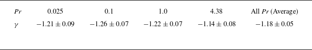


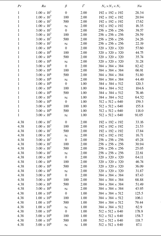


 Open access