


Non-technical Summary
Ammonoids and other externally shelled cephalopods were vital components of marine ecosystems for nearly half a billion years, but their swimming capabilities and ecological roles are not well understood. Additionally, these animals often had elaborate projections on their shells (i.e., ornamentation patterns) that became more common throughout their evolutionary history. Anti-predatory roles have been traditionally invoked to support this relative increase in ornamentation intensity and abundance. However, this role does not adequately explain the function or adaptive value for many forms of conch ornamentation. We present a cross-disciplinary approach to investigate these ornamentation patterns from a hydromechanical perspective, using a combination of virtual and physical experiments. These experiments involve (1) generating theoretical morphologies from nearly 200 fossil specimens to isolate biologically relevant variables; (2) using 3D modeling to compute hydrostatic properties (buoyancy, mass balance, passive stability); (3) using weighted, 3D-printed models to characterize how ornamentation attenuates rocking behavior; (4) using flow visualization experiments (particle image velocimetry) to explore the hydrodynamic mechanisms underpinning rocking attenuation; and (5) using computer simulations to understand the cost of ornamentation patterns during linear swimming (i.e., computational fluid dynamics). Coarser ornamentation patterns attenuate rocking behavior, serving as a dynamic stability mechanism. While the coarsest shells incur extra drag during swimming, intermediate forms do not, suggesting that some morphologies effectively avoid this physical trade-off. These relationships highlight important selective pressures involved in the evolutionary history of ammonoid cephalopods.
Introduction
Externally shelled cephalopods (ectocochleates) displayed a remarkable variety of conch shapes and sizes throughout their extensive evolutionary history (Arkell et al. Reference Arkell, Furnish, Kummel, Miller, Moore, Schindewolf, Sylvester-Bradley, Wright, of and Moore1957; Teichert et al. Reference Teichert, Kummel, Sweet, Stenzel, Furnish, Glenister, Erben, Moore, Zeller and Moore1964; Raup Reference Raup1967; Wright et al. Reference Wright, Calloman, Howarth, of and Kaesler1996; Korn and Klug Reference Korn, Klug and Talent2012; Klug et al. Reference Klug, De Baets and Korn2016; Hoffmann et al. Reference Hoffmann, Slattery, Kruta, Linzmeier, Lemanis, Mironenko, Goolaerts, De Baets, Peterman and Klug2021), spanning around half a billion years (Kröger et al. Reference Kröger, Vinther and Fuchs2011; Pohle et al. Reference Pohle, Kröger, Warnock, King, Evans, Aubrechtova, Cichowolski, Fang and Klug2022). The conch (referring to the entire geometry of the shell) offered some degree of protection against predators, while also serving as a chambered buoyancy apparatus (Hoffmann et al. Reference Hoffmann, Lemanis, Naglik, Klug, Klug, Korn, De Baets, Kruta and Mapes2015). Conch morphology placed fundamental constraints on how these living animals navigated their physical environments. Additionally, their vast fossil record documents how cephalopod conch morphologies have been shaped by selection across myriad global and local extinction events. A better understanding of their hydromechanical properties would provide key context to the life habits and ecology of organisms that dominated many marine ecosystems around the globe. More broadly, the evolutionary biomechanics of these animals illuminate unique solutions to obstacles presented by underwater locomotion involving buoyancy, stability (in static and dynamic settings), maneuverability, passive and active orientation control, and locomotive efficiency (Trueman Reference Trueman1940; Saunders and Shapiro Reference Saunders and Shapiro1986; Chamberlain Reference Chamberlain1990, Reference Chamberlain1993; Jacobs Reference Jacobs1992; Jacobs and Chamberlain Reference Jacobs, Chamberlain, Landman, Tanabe and Davis1996; Hoffmann et al. Reference Hoffmann, Lemanis, Naglik, Klug, Klug, Korn, De Baets, Kruta and Mapes2015; Naglik et al. Reference Naglik, Tajika, Chamberlain, Klug, Klug, Korn, De Baets, Kruta and Mapes2015; Peterman et al. Reference Peterman, Ciampaglio, Shell and Yacobucci2019, Reference Peterman, Hebdon, Ciampaglio, Yacobucci, Landman and Linn2020a,Reference Peterman and Ritterbushb,Reference Peterman, Shell, Ciampaglio and Yacobuccic; Morón-Alfonso et al. Reference Morón-Alfonso, Peterman, Cichowolski, Hoffmann and Lemanis2021; Peterman and Ritterbush Reference Peterman and Ritterbush2021, Reference Peterman and Ritterbush2022a,Reference Peterman and Ritterbushb; Hebdon et al. Reference Hebdon, Polly, Peterman and Ritterbush2022a,Reference Hebdon, Ritterbush, Choi and Petermanb; De Blasio Reference De Blasio2023).
Ammonoid Conch Ornamentation—Evolutionary Patterns and Functional Hypotheses
Compared with earlier stem-group cephalopods and contemporaneous nautiloids, ammonoids displayed higher disparity in shell sculptures superimposed on their first-order conch shapes (Arkell et al. Reference Arkell, Furnish, Kummel, Miller, Moore, Schindewolf, Sylvester-Bradley, Wright, of and Moore1957; Teichert et al. Reference Teichert, Kummel, Sweet, Stenzel, Furnish, Glenister, Erben, Moore, Zeller and Moore1964). These second-order morphological features are termed “ornamentation,” describing any number of projections or depressions (spines, ribs or costae, lirae, tubercles, clavi, nodes, varices, apertural constrictions, furrows, carinae, etc.; for descriptions, see Arkell et al. Reference Arkell, Furnish, Kummel, Miller, Moore, Schindewolf, Sylvester-Bradley, Wright, of and Moore1957; Teichert et al. Reference Teichert, Kummel, Sweet, Stenzel, Furnish, Glenister, Erben, Moore, Zeller and Moore1964; Klug et al. Reference Klug, Korn, Landman, Tanabe, De Baets, Naglik, Klug, Korn, De Baets, Kruta and Mapes2015). While there is much morphological disparity among ornamentation patterns, each category would have contributed to the roughness of ammonoid conchs and their topological complexity. That is, each of these patterns would have modulated the physical properties of an ammonoid’s first-order shape, complicating our understanding of functional morphology and syn vivo swimming capabilities.
Across a variety of organisms, ornamentation patterns or similar projections can serve many different functional roles. Predator deterrence has been suggested for some ammonoids (Ward Reference Ward1981; Kröger Reference Kröger2002), gastropods (Vermeij Reference Vermeij1987, Reference Vermeij2002), bivalves (Harper and Kelley Reference Harper and Kelley2012; Klompmaker and Kelley Reference Klompmaker and Kelley2015), brachiopods (Alexander Reference Alexander1986), and crinoids (Brett and Walker Reference Brett and Walker2002), with projections potentially increasing a predator’s required gape size, causing difficulty handling prey items, or otherwise inflicting pain (Alexander Reference Alexander1986; Donovan et al. Reference Donovan, Danko and Carefoot1999; Savazzi Reference Savazzi1999; Brett and Walker Reference Brett and Walker2002; Harper and Kelley Reference Harper and Kelley2012). Conversely, these patterns in brachiopods and bivalves may have reduced sediment scour while improving burrowing capabilities or anchoring on or within a substrate (Bottjer and Carter Reference Bottjer and Carter1980; Stanley Reference Stanley1981; Savazzi Reference Savazzi1999; Harper and Kelley Reference Harper and Kelley2012; Garcia et al. Reference Garcia, Molinaro and Leighton2018). Many projections can have positive hydrodynamic effects. Tubercles on the leading edge of whale flippers improve lift generation and maneuverability (Fish et al. Reference Fish, Weber, Murray and Howle2011), spines on microplankton have been demonstrated to reduce sinking rates (Padisák et al. Reference Padisák, Soróczki-Pintér and Rezner2003), and ribs on ammonoids have been suggested to decrease hydrodynamic drag depending upon size (Chamberlain and Westermann Reference Chamberlain and Westermann1976). Finally, ornamentation serving as camouflage or for sexual display, while difficult to determine for extinct organisms, has been demonstrated for extant marine animals (Bottjer and Carter Reference Bottjer and Carter1980; Summers and Ord Reference Summers and Ord2021). For a more detailed reading of invertebrate ornamentation and functional morphology see Savazzi (Reference Savazzi1999), Seilacher and Gishlick (Reference Seilacher and Gishlick2014), and Klompmaker et al. (Reference Klompmaker, Kelley, Chattopadhyay, Clements, Huntley and Kowalewski2019).
Evolutionary patterns documented by the fossil record can shed light on the ecological and functional significance of conch ornamentation. First, the proportion of ammonoid conchs with ornamentation generally increased throughout the evolutionary history of this clade (Ward Reference Ward1981; Fig. 1). Second, ornamentation intensity increased, with the relative abundance of intermediate and coarsely ornamented conchs becoming more common, especially during the Mesozoic (Ward Reference Ward1981; Fig. 1). These evolutionary patterns have been interpreted as adaptive responses during the Mesozoic marine revolution (Vermeij Reference Vermeij1977, Reference Vermeij2002; Ward Reference Ward1981; Kerr and Kelley Reference Kerr and Kelley2015). This event involved fundamental reorganizations of marine invertebrate communities in response to the radiation of durophagous animals (e.g., crustaceans, teleosts, and chondrichthyans) and the diversification of predatory strategies (Vermeij Reference Vermeij1987; Walker and Brett Reference Walker and Brett2002; Aberhan et al. Reference Aberhan, Kiessling and Fürsich2006; Baumiller et al. Reference Baumiller, Salamon, Gorzelak, Mooi, Messing and Gahn2010; Buatois et al. Reference Buatois, Carmona, Curran, Netto, Mángano, Wetzel, Mángano and Buatois2016; Klompmaker et al. Reference Klompmaker, Kelley, Chattopadhyay, Clements, Huntley and Kowalewski2019). These pressures presumably selected for anti-predatory morphologies; an evolutionary response known as escalation (Vermeij Reference Vermeij1987). However, the majority of ammonoid ornamentation patterns lack clear defensive roles.
A, Relative frequency of Mesozoic ammonoids belonging to four different coarseness categories (data adapted from Ward Reference Ward1981; representative ammonoid photos used with permission from the Treatise on Invertebrate Paleontology, Part L, Wright et al. Reference Wright, Calloman, Howarth, of and Kaesler1996). B–F, Examples of various ornamentation patterns. B, Fine costae that bifurcate toward the venter (Dactylioceras commune [Sowerby Reference Sowerby1815]; YPM IP 522750). C, Coarse ornamentation patterns with a smooth venter (Asteroceras obtusum [Sowerby Reference Sowerby1817]; YPM IP 6170). D, Very coarse ornamentation patterns (Dunveganoceras pondi Haas Reference Haas1949; YPM IP 10162). E, Prominent ventrolateral spines (Eteoderoceras obesum [Spath Reference Spath1929], National Museum of Wales #60.510.G4326). F, Medially asymmetrical costae (Hoplitidae; UMNH IP 4621; Courtesy of the Natural History Museum of Utah; UMNH). G, Ventrolateral tubercles superimposed on fine costae (Hoploscaphites nodosus [Owen Reference Owen1852]; AMNH-FI-58513; courtesy of AMNH). Scale bars, 5 cm. All photos are used with permission from their respective repositories.

Forms of conch ornamentation invoked for defensive roles each have alternate explanations. The simplest way to improve shell strength is to increase its thickness. However, rather than thickening the shell, most ornamentation patterns result from flaring of the aperture during accretionary growth, with the internal shell interface often resembling the external topology (Kennedy and Cobban Reference Kennedy and Cobban1976; Bucher et al. Reference Bucher, Landman, Klofak, Guex, Landman, Tanabe and Davis1996; Wright et al. Reference Wright, Calloman, Howarth, of and Kaesler1996). These “hollow” patterns may be by-products of morphogenetic constraints or may reduce the demands imposed by buoyancy and biomineralization. While some spiny features seem robust enough to ward off smaller predators (Fig. 1E), many well-preserved spinose conchs have rather delicate spines with hollow (but often septate) morphologies (Kennedy and Cobban Reference Kennedy and Cobban1976). Furthermore, some hollow spines have even been proposed to serve a sensory function in some clades (Checa and Martin-Ramos Reference Checa and Martin-Ramos1989; Ifrim et al. Reference Ifrim, Bengtson and Schweigert2018). Alternate anti-predator roles can involve evasion rather than defense. Accordingly, some ornamentation patterns have been proposed to serve as camouflage; breaking up sharp lines from the silhouettes of the smooth conchs, or blending in with structural features on the seafloor (Cowen et al. Reference Cowen, Gertman and Wiggett1973; Kennedy and Cobban Reference Kennedy and Cobban1976; Westermann Reference Westermann, Landman, Tanabe and Davis1996, Reference Westermann and Savazzi1998; Seilacher and Gishlick Reference Seilacher and Gishlick2014). Transverse ornamentation (e.g., costae, varices, and apertural restrictions) has been suggested to minimize fractures by redirecting them parallel to the aperture (Simoulin Reference Simoulin1945; Ward Reference Ward1981; Checa and Westermann Reference Checa and Westermann1989). Other hypotheses concerning these transverse patterns involve ornamentation stiffening the conch (Spath Reference Spath1919; Rangheard and Theobald Reference Rangheard and Theobald1961; Westermann Reference Westermann1971; Hewitt Reference Hewitt, Landman, Tanabe and Davis1996; Seilacher and Gishlick Reference Seilacher and Gishlick2014), or creating internal structure, preventing the soft body from being pulled out of the body chamber (Obata et al. Reference Obata, Futakami, Kawashita and Takahashi1978). While corrugated structures can gain mechanical benefits (Pennington and Currey Reference Pennington and Currey1984; Alexander Reference Alexander1990), such hypotheses have yet to be tested on real ammonoid morphologies in the context of solid mechanics. Finally, these animals retain their entire ontogeny due to their accretionary growth, meaning the earlier whorls (when exposed) are considerably thinner and weaker than the rest of the shell. This inherently weak region obscures analogies with other corrugated mollusk shells (e.g., scallops). In short, escalation of anti-predatory defense is insufficient to explain the increased relative abundance of ornamented ammonoids during the Mesozoic.
Sublethal injuries shed light on cephalopod predator–prey interactions in the fossil record. These pathologies are commonly preserved in cephalopod fossils and were produced by a variety of mechanisms: peeling predators, parasites, mantle damage, struggles with prey, and possibly mating (Arnold Reference Arnold1985; Landman and Waage Reference Landman and Waage1986; Hengsbach Reference Hengsbach, Landman, Tanabe and Davis1996; Checa et al. Reference Checa, Okamoto and Keupp2002; Kennedy et al. Reference Kennedy, Cobban and Klinger2002; Klug Reference Klug2007; Keupp Reference Keupp2012; Hoffmann and Keupp Reference Hoffmann, Keupp, Klug, Korn, De Baets, Kruta and Mapes2015). Sublethal injuries reveal whether an individual was able to survive an attack and can serve as indices of predation frequency and survivorship for particular prey phenotypes (Vermeij et al. Reference Vermeij, Schindel and Zipser1981; Vermeij Reference Vermeij1982; Landman and Waage Reference Landman and Waage1986; West et al. Reference West, Cohen and Baron1991; Kröger Reference Kröger2002; Dietl and Kosloski Reference Dietl and Kosloski2013; Kerr and Kelley Reference Kerr and Kelley2015). Kerr and Kelley (Reference Kerr and Kelley2015) found that finely ribbed ammonoids had higher repair frequencies compared with coarsely ornamented ammonoids, suggesting that finely ribbed ammonoids were more frequently preyed upon, more often survived predator attacks, or were more likely to encounter predators. An alternative strategy to increase survivorship is to simply increase shell thickness. The effectiveness of this strategy is supported by thicker-shelled taxa having higher repair frequencies, with thin-shelled taxa more often succumbing to predation (Bond and Saunders Reference Bond and Saunders1989). While predation frequency has been confirmed to increase from the Jurassic to Cretaceous (Kerr and Kelley Reference Kerr and Kelley2015), the abovementioned patterns do not sufficiently explain the increase in ornamented morphologies during this time (especially coarser ones), suggesting that these synecological pressures only explain selection for some subset of ornamentation patterns.
Morphological patterns of covariation (i.e., Buckman’s rules of covariation; De Baets et al. Reference De Baets, Bert, Hoffmann, Monnet, Yacobucci, Klug, Klug, Korn, De Baets, Kruta and Mapes2015; Monnet et al. Reference Monnet, De Baets, Yacobucci, Klug, Korn, De Baets, Kruta and Mapes2015a) can also help rank the selective agents acting on ammonoid conch ornamentation. While these rules generally apply to intraspecific patterns, they can also be observed above the species level. This covariation of morphological features may also correspond to the covariation of certain physical properties. Openly whorled conchs (evolutes) have been reported to express coarser ornamentation (De Baets et al. Reference De Baets, Bert, Hoffmann, Monnet, Yacobucci, Klug, Klug, Korn, De Baets, Kruta and Mapes2015; Monnet et al. Reference Monnet, De Baets, Yacobucci, Klug, Korn, De Baets, Kruta and Mapes2015a). If these patterns represent ecophenotypes, they may express different morphologies according to different environmental conditions (e.g., lithofacies indicative of distal vs. proximal oceanographic settings; Westermann Reference Westermann, Landman, Tanabe and Davis1996; De Baets et al. Reference De Baets, Bert, Hoffmann, Monnet, Yacobucci, Klug, Klug, Korn, De Baets, Kruta and Mapes2015). More evolute, ornamented forms are commonly reported for individuals recovered from more distal settings (Jacobs et al. Reference Jacobs, Landman and Chamberlain1994; Jacobs and Chamberlain Reference Jacobs, Chamberlain, Landman, Tanabe and Davis1996; Westermann Reference Westermann, Landman, Tanabe and Davis1996, Reference Westermann and Savazzi1998; Kawabe Reference Kawabe2003; De Baets et al. Reference De Baets, Bert, Hoffmann, Monnet, Yacobucci, Klug, Klug, Korn, De Baets, Kruta and Mapes2015; Monnet et al. Reference Monnet, De Baets, Yacobucci, Klug, Korn, De Baets, Kruta and Mapes2015a), but opposite patterns (Wilmsen and Mosavinia Reference Wilmsen and Mosavinia2011) and more ambiguous patterns have also been reported (Batt Reference Batt1989; Courville and Thierry Reference Courville and Thierry1993; Kawabe Reference Kawabe2003). In either case, associations between conch geometry and ornamentation display a surprising amount of phenotypic plasticity. For example, genera such as Amaltheus Montfort, Reference Montfort1808, Neogastroplites McLearn, Reference McLearn1931, Schloenbachia Neumayr, Reference Neumayr1875, and Collignoniceras Breistroffer, Reference Breistroffer1947 display gradations in coiling and ornamentation that are so extreme, different individuals might seem to be separate species at first glance (Kennedy et al. Reference Kennedy, Cobban and Landman2001; Yacobucci Reference Yacobucci2004; Hammer and Bucher Reference Hammer and Bucher2006; Wilmsen and Mosavinia Reference Wilmsen and Mosavinia2011). Each of these trends support some functional value for these ubiquitous ornamentation patterns, or alternatively, a release from particular selective pressures in certain environments (Kennedy and Cobban Reference Kennedy and Cobban1976).
Some aspects of conch ornamentation may also have arisen from chemical and physical morphogenetic constraints (Checa and Martin-Ramos Reference Checa and Martin-Ramos1989; Hammer and Bucher Reference Hammer and Bucher1999; Erlich et al. Reference Erlich, Moulton, Goriely and Chirat2016; Ifrim et al. Reference Ifrim, Bengtson and Schweigert2018; Schoeppler et al. Reference Schoeppler, Lemanis, Reich, Pusztai, Gránásy and Zlotnikov2019). Some features may have been solely morphogenetic (i.e., fabricational noise; Seilacher Reference Seilacher1973; Bucher et al. Reference Bucher, Chirat and Guex2003), although this mechanism seems inadequate to explain the breadth and intensity of ornamentation patterns among ammonoids. Conch ornamentation is also partially constrained by phylogeny, with certain groups more likely to express diagnostic ornamentation patterns (e.g., Acanthoceratoidea, Eoderoceratoidea, Hoplitidae, Aspidoceratidae, Arietitidae, various heteromorph clades, and many others; Westermann Reference Westermann, Landman, Tanabe and Davis1996; Wright et al. Reference Wright, Calloman, Howarth, of and Kaesler1996; Hoffmann et al. Reference Hoffmann, Slattery, Kruta, Linzmeier, Lemanis, Mironenko, Goolaerts, De Baets, Peterman and Klug2021). Any one morphology reflects the mixed constraints of these functional, ecological, phylogenetic, and morphogenetic factors (Seilacher and Gishlick Reference Seilacher and Gishlick2014). Therefore, all conch ornamentation cannot be generally explained through any singular mechanism, and likely represents an adaptive compromise between several functional and nonfunctional factors (Chamberlain and Westermann Reference Chamberlain and Westermann1976).
Hydromechanics of Ectocochleate Cephalopods
Hydromechanical properties likely served as important selective agents for some forms of conch ornamentation. Conch shape has been found to severely constrain syn vivo swimming capabilities (e.g., drag, lift, dynamic stability, maneuverability, locomotion efficiency; Denton Reference Denton1974; Chamberlain Reference Chamberlain1976, Reference Chamberlain, House and Senior1981, Reference Chamberlain1993; Jacobs Reference Jacobs1992; Jacobs et al. Reference Jacobs, Landman and Chamberlain1994; Jacobs and Chamberlain Reference Jacobs, Chamberlain, Landman, Tanabe and Davis1996; Naglik et al. Reference Naglik, Tajika, Chamberlain, Klug, Klug, Korn, De Baets, Kruta and Mapes2015; Hebdon et al. Reference Hebdon, Ritterbush and Choi2020, Reference Hebdon, Ritterbush and Choi2021, Reference Peterman and Ritterbush2022a,Reference Hebdon, Ritterbush, Choi and Petermanb, Peterman et al. Reference Peterman, Hebdon, Ciampaglio, Yacobucci, Landman and Linn2020a,Reference Peterman, Shell, Ciampaglio and Yacobuccic, Reference Peterman, Hebdon, Shell, Ritterbush, Slattery, Larson, Bingle-Davis and Bingle-Davis2022; Peterman and Ritterbush Reference Peterman and Ritterbush2021, Reference Peterman and Ritterbush2022a,Reference Peterman and Ritterbushb; Ritterbush and Hebdon Reference Ritterbush and Hebdon2023). Compressed, involute conchs (oxycones) generally incur less drag than similarly sized inflated or evolute forms (sphaerocones and serpenticones, respectively; Jacobs Reference Jacobs1992; Jacobs et al. Reference Jacobs, Landman and Chamberlain1994; Hebdon et al. Reference Hebdon, Ritterbush and Choi2020, Reference Hebdon, Ritterbush and Choi2021; Ritterbush and Hebdon Reference Ritterbush and Hebdon2023), especially at higher Reynolds numbers (i.e., the ratio between inertial forces and viscous forces; >~2000; Hebdon et al. Reference Hebdon, Ritterbush and Choi2020). Oxycones were more often smooth and streamlined, whereas Jurassic–Cretaceous evolute and inflated morphologies were more likely to have some form of ornamentation (Arkell et al. Reference Arkell, Furnish, Kummel, Miller, Moore, Schindewolf, Sylvester-Bradley, Wright, of and Moore1957; Kennedy and Cobban Reference Kennedy and Cobban1976; Wright et al. Reference Wright, Calloman, Howarth, of and Kaesler1996). Coarser ornamentation patterns may have increased drag (Kummel and Lloyd Reference Kummel and Lloyd1955; Chamberlain and Westermann Reference Chamberlain and Westermann1976; Kennedy and Cobban Reference Kennedy and Cobban1976; Checa and Westermann Reference Checa and Westermann1989), leading to interpretations of the ammonoids bearing these conchs as poor swimmers (Westermann Reference Westermann1971, Reference Westermann, Landman, Tanabe and Davis1996, Reference Westermann and Savazzi1998; Batt Reference Batt1989; Seilacher and Gishlick Reference Seilacher and Gishlick2014). In the context of a global Mesozoic marine revolution, increased swimming cost from strongly ornamented conchs has been cast as an unfortunate downside to their necessary acquisition of anti-predator features. But if these ornamentation patterns were not chiefly anti-predatory, it becomes difficult to understand an adaptive role for features that would presumably hamper swimming and general locomotion efficiency.
More nuanced interactions between ammonoid conchs and fluids have been proposed. Some patterns have been suggested to stabilize the conch while swimming by directing fluid along the flanks (Jacobs and Chamberlain Reference Jacobs, Chamberlain, Landman, Tanabe and Davis1996), although this role has not been quantitatively evaluated. Some ornamentation patterns (i.e., fine costae) have also been suggested to act similarly to dimples on golf balls, reducing pressure drag on the trailing end by preventing flow separation (Chamberlain and Westermann Reference Chamberlain and Westermann1976; Jacobs and Chamberlain Reference Jacobs, Chamberlain, Landman, Tanabe and Davis1996; Kundu et al. Reference Kundu, Cohen and Dowling2016). The emerging use of computational techniques in paleobiology, like computational fluid dynamics (CFD), can help illuminate outstanding questions concerning hydrodynamics, especially when using theoretical morphologies to isolate variables (e.g., Hebdon et al. Reference Hebdon, Ritterbush and Choi2020, Reference Hebdon, Ritterbush and Choi2021, Reference Hebdon, Polly, Peterman and Ritterbush2022a,Reference Hebdon, Ritterbush, Choi and Petermanb; Peterman and Ritterbush Reference Peterman and Ritterbush2022a,Reference Peterman and Ritterbushb; Ritterbush and Hebdon Reference Ritterbush and Hebdon2023). Earlier experiments demonstrate that the fine ribs and tubercles on scaphitid ammonoids increase drag by a factor of ~1.14 compared with a theoretical smooth shape (Peterman et al. Reference Peterman, Hebdon, Ciampaglio, Yacobucci, Landman and Linn2020a). Conversely, vertical swimming experiments on ornamented and smooth models of helicospiral ammonoids did not reveal any detectable differences in kinematics (Peterman et al. Reference Peterman, Hebdon, Shell, Ritterbush, Slattery, Larson, Bingle-Davis and Bingle-Davis2022). These experiments highlight the need for a broad, generalizable range of theoretical morphologies to test hypotheses concerning functional morphology.
Hydrostatics (i.e., buoyancy and mass balance) add more complexity to the locomotive constraints of an ectocochleate cephalopod. While external topology influences hydrodynamics, both coiling geometry and internal characteristics influence these hydrostatic properties. The gas-filled, chambered conch (phragmocone) maintains a condition close to neutral buoyancy by compensating for organismal mass throughout growth (Trueman Reference Trueman1940; Denton and Gilpin-Brown Reference Denton and Gilpin-Brown1966; Heptonstall Reference Heptonstall1970; Chamberlain Reference Chamberlain, House and Senior1981; Greendwald and Ward Reference Greendwald, Ward, Saunders and Landman1987; Jacobs and Chamberlain Reference Jacobs, Chamberlain, Landman, Tanabe and Davis1996; Hoffmann et al. Reference Hoffmann, Lemanis, Naglik, Klug, Klug, Korn, De Baets, Kruta and Mapes2015; Peterman et al. Reference Peterman, Mikami and Inoue2020b). The relative locations of the centers of buoyancy and mass place fundamental constraints on the life habits and swimming capabilities of these animals. The center of buoyancy is the center of volume of the water displaced by the living animal, whereas the center of mass is a weighted average, depending upon the distribution of each material of unique density that composes the animal (Hoffmann et al. Reference Hoffmann, Lemanis, Naglik, Klug, Klug, Korn, De Baets, Kruta and Mapes2015; Peterman and Ritterbush Reference Peterman and Ritterbush2022b). The passive, stable orientation of these living animals occurs when the centers of buoyancy and mass are vertically aligned (Denton Reference Denton1974; Saunders and Shapiro Reference Saunders and Shapiro1986; Klug and Korn Reference Klug and Korn2004; Hoffmann et al. Reference Hoffmann, Lemanis, Naglik, Klug, Klug, Korn, De Baets, Kruta and Mapes2015). Separation of these hydrostatic centers governs hydrostatic stability, as well as the difficulty or ease of modifying orientation (i.e., maneuverability; Raup Reference Raup1967; Raup and Chamberlain Reference Raup and Chamberlain1967; Saunders and Shapiro Reference Saunders and Shapiro1986; Hoffmann et al. Reference Hoffmann, Lemanis, Naglik, Klug, Klug, Korn, De Baets, Kruta and Mapes2015; Lemanis et al. Reference Lemanis, Zachow, Fusseis and Hoffmann2015; Tajika et al. Reference Tajika, Naglik, Morimoto, Pascual-Cebrian, Hennhöfer and Klug2015; Naglik et al. Reference Naglik, Rikhtegar and Klug2016; Peterman et al. Reference Peterman, Ciampaglio, Shell and Yacobucci2019, Reference Peterman, Shell, Ciampaglio and Yacobucci2020c, Peterman and Ritterbush Reference Peterman and Ritterbush2022a,Reference Peterman and Ritterbushb). Finally, the separation between these hydrostatic centers and their locations relative to the source of jet thrust (the hyponome) constrains the directional efficacy of thrusting. A larger proportion of thrust energy is transmitted into movement in some direction when the thrust vector passes through the hydrostatic centers (i.e., the thrust angle; Jacobs and Chamberlain Reference Jacobs, Chamberlain, Landman, Tanabe and Davis1996; Okamoto Reference Okamoto, Landman, Tanabe and Davis1996; Klug and Korn Reference Klug and Korn2004; Naglik et al. Reference Naglik, Tajika, Chamberlain, Klug, Klug, Korn, De Baets, Kruta and Mapes2015; Peterman et al. Reference Peterman, Hebdon, Ciampaglio, Yacobucci, Landman and Linn2020a,Reference Peterman, Mikami and Inoueb,Reference Aberhan, Kiessling and Fürsichc, Reference Peterman, Hebdon, Shell, Ritterbush, Slattery, Larson, Bingle-Davis and Bingle-Davis2022; Peterman and Ritterbush Reference Peterman and Ritterbush2021). Increased misalignment of the thrust vector will transmit more energy into rotation rather than locomotion, with less hydrostatically stable forms being more sensitive to jetting at the proper thrust angle (measured between two lines that connect the horizontal plane and source of jet thrust with the midpoint between the hydrostatic centers). Hydrostatic stability may also constrain the timing of each jet pulse, coordinating them with the rocking induced by jetting (De Blasio Reference De Blasio2023). Adding ornament by corrugating or flaring the aperture, or by thickening the shell, would increase the mass of the conch, thus influencing buoyancy and the distribution of organismal mass to some extent (Teichert Reference Teichert, Teichert and Yochelson1967; Westermann Reference Westermann1971; Kennedy and Cobban Reference Kennedy and Cobban1976). Ultimately, hydrostatic properties place fundamental physical constraints on locomotion and are coupled with the abovementioned hydrodynamic properties to yield some range of swimming capabilities for any particular morphology.
Ectocochleates likely encountered numerous functional trade-offs throughout their evolutionary history. We hypothesize that conch ornamentation was subject to physical trade-offs between dynamic stability (i.e., rocking attenuation) and hydrodynamic efficiency. To evaluate these hydromechanical properties, we use idealized theoretical morphologies falling on a continuum of increasing ornamentation coarseness (Fig. 2). Using a mixture of computational and physical models, we investigate the fundamental constraints on swimming capabilities imposed by conch ornament, including: (1) the degree to which ornamentation influences hydrostatics (buoyancy and mass balance), (2) the degree to which ornamentation attenuates rocking (serving as a dynamic stability mechanism), (3) the efficacy of rocking attenuation for different hydrostatic stabilities, (4) the hydrodynamic costs of ornamentation across a biologically relevant range of scales, and (5) whether fine ornamentation improves hydrodynamic efficiency across some range of scales. Finally, we compare these hydromechanical properties to patterns documented in the fossil record to better understand the life habits and ecological roles of ectocochleate cephalopods and the physical constraints on aquatic locomotion more broadly.
Theoretical ammonoid morphologies falling on a continuum of increasing ornamentation coarseness (left to right: smooth, fine, medium, coarse, and very coarse). Here, coarser ornamentation refers to patterns with higher amplitude and lower frequency (where smooth shells can be regarded as having zero amplitude and infinitely high frequency). The green portion of each model represents the soft body of the living animal, while the remainder of the shell is the chambered phragmocone. The tips of the blue and red cones denote the positions of the centers of buoyancy and mass, respectively.

Methods
Design of Theoretical Morphologies
Theoretical morphologies were generated to investigate the hydromechanics of conch ornamentation. This approach allows conch ornamentation to be an isolated variable, while holding shell coiling and other nuanced morphological features constant (shell and septal thickness, body chamber length, and septal morphology). Four ornamented models with progressively coarser ornamentation were created by adding ornamentation to a smooth (control) model. These models fall in the direct center of the Westermann morphospace (Ritterbush and Bottjer Reference Ritterbush and Bottjer2012), a ternary diagram contrasting whorl expansion (W; widening of the shell tube during each half whorl; Supplementary Equation S1) umbilical exposure (U; the degree of exposure for the earlier whorls; Supplementary Equation S2), and inflation (Th; width to diameter ratio; Supplementary Equation S3). A conch with these parameters (Supplementary Table S1) was constructed following earlier methods (Peterman and Ritterbush Reference Peterman and Ritterbush2022a) involving the use of arrays in the open-source modeling program Blender (Blender Documentation Team 2019). These arrays successively copy, translate, rotate, and scale an adult whorl section, producing a 3D shell tube after bridging together all copies (Supplementary Table S2). A diameter of 17.5 cm for the first-order conch morphology was held constant for all five models.
Ornamentation was quantified by measuring 187 ammonoid species from 52 families spanning the Jurassic and Cretaceous. Specimens were measured from the Treatise on Invertebrate Paleontology (Arkell et al. Reference Arkell, Furnish, Kummel, Miller, Moore, Schindewolf, Sylvester-Bradley, Wright, of and Moore1957; Wright et al. Reference Wright, Calloman, Howarth, of and Kaesler1996), the Yale Peabody Museum (YPM), and the Natural History Museum of Utah (UMNH). Westermann parameters (W, U, and Th), ornamentation amplitude, and ornamentation spacing were recorded from each individual. Specimen names (family, genus, and species), time periods, figure numbers (for Treatise specimens), specimen numbers (for museum specimens), and all measurements are listed in Supplementary Dataset S1 (https://doi.org/10.5281/zenodo.15596786). Museum specimens were measured with digital calipers and a depth gauge (for YPM specimens), and directly from 3D scans using an Artec Space Spider (for UMNH specimens). Specimens figured in the Treatise on Invertebrate Paleontology (Arkell et al. Reference Arkell, Furnish, Kummel, Miller, Moore, Schindewolf, Sylvester-Bradley, Wright, of and Moore1957; Wright et al. Reference Wright, Calloman, Howarth, of and Kaesler1996) were measured in ImageJ (Schneider et al. Reference Schneider, Rasband and Eliceiri2012). These measurements are sensitive to the medial plane of the fossil being oriented orthogonally to the camera view. Furthermore, error in measurements can arise depending on specimen preservation (i.e., internal molds, abraded ribs, etc.). Despite these sources of measurement error, the theoretical morphologies generated from these data still span the majority of biologically relevant ornamentation coarseness values.
Reducing a complex topology to a single number inevitably results in the loss of information. However, these measured specimens serve the purpose of characterizing general ornamentation coarseness across the morphospace (Fig. 3) and inform the design of the theoretical morphologies used for the current experiments. Ornamentation amplitude was measured as the amount protruding above the whorl height of the first-order geometry along the venter or ventral shoulder (the highest-value regions). Ornamentation spacing was measured as the angle between two successive ornamentation patterns (e.g., adjacent ribs or costae), with the vertex at the coiling axis of the conch. Coarser patterns are defined here as generally having larger amplitude and spacing. Therefore, we introduce a dimensionless coarseness index (Ic):
 $$ {\mathrm{I}}_{\mathrm{c}}=\frac{\left({A}_{\mathrm{orn}}/\mathrm{Wh}\right)}{\left(360/{\unicode{x03B8}}_{\mathrm{orn}}\right)} $$
Ornamentation amplitude (A), spacing (B), and coarseness index (Ic; eq. 1) (C) plotted on the Westermann morphospace (a ternary diagram where the bottom, left, and right corners represent conchs with high whorl expansion, umbilical exposure, and lateral inflation, respectively; see Ritterbush and Bottjer Reference Ritterbush and Bottjer2012). Coarseness indices have been binned into arbitrary categories to distinguish five different levels of ornamentation coarseness. These measurements informed the design of theoretical morphologies that isolate the variable of ornamentation coarseness (see Fig. 1).

where A orn is the ornament amplitude, Wh is the whorl height (measured from the umbilical seam to the venter), and θorn is the ornament spacing. Note the denominator is equal to the ornament frequency per whorl. Both A orn and θorn are averaged from five measurements on the outer whorl of each specimen. Smooth specimens were designated an infinitely small ornamentation spacing, allowing Ic values approaching zero to represent smooth conchs and larger values to represent coarser conchs. Note that specimens incompatible with this index (i.e., smooth venters, mixtures of spines and ribs) were ignored, introducing sampling bias. The current sample of ornamented ammonoids shows that the ratio of amplitude to spacing follows a normal distribution (Supplementary Fig. S1), with a mode of ~5.5 × 10⁻³. This value was used in the theoretical models to maintain the ornamentation amplitude to spacing ratio across a spectrum of coarseness indices.
Ornamentation patterns were generated as simple costae in the shape of a perfect sine wave at the venter with a height to width ratio of 1:2. Toward the umbilical seam, costae gradually attenuate to zero amplitude. Coarseness indices spanning the range of the measured ammonoids (Supplementary Dataset S1) were chosen for the theoretical morphologies (ranging nearly three orders of magnitude; Table 1). These ornamentation patterns were replicated using the same sets of instructions to build the shell using the program Blender (Blender Documentation Team 2019). We chose five morphologies with increasing ornament coarseness: smooth (control; $ {\mathrm{I}}_{\mathrm{c}}=0 $
), fine (
$ {\mathrm{I}}_{\mathrm{c}}=0 $
), fine ( $ {\mathrm{I}}_{\mathrm{c}} $
= 0.0611), medium (
$ {\mathrm{I}}_{\mathrm{c}} $
= 0.0611), medium ( $ {\mathrm{I}}_{\mathrm{c}} $
= 1.24), coarse (
$ {\mathrm{I}}_{\mathrm{c}} $
= 1.24), coarse ( $ {\mathrm{I}}_{\mathrm{c}} $
= 4.95), and very coarse (
$ {\mathrm{I}}_{\mathrm{c}} $
= 4.95), and very coarse ( $ {\mathrm{I}}_{\mathrm{c}} $
= 19.8). Examples of conch and ornamentation measurements are shown in the Supplementary Information (Supplementary Information Methods, Supplementary Fig. S13).
$ {\mathrm{I}}_{\mathrm{c}} $
= 19.8). Examples of conch and ornamentation measurements are shown in the Supplementary Information (Supplementary Information Methods, Supplementary Fig. S13).
Various morphological and physical properties of five theoretical morphologies with increasing ornamentation coarseness. A orn/W h = ornament amplitude to whorl height ratio; θorn = ornamentation angular spacing; Ic = ornamentation coarseness index; BCL = angular body chamber length; Φ = percentage of the chambered shell (phragmocone) to be emptied for neutral buoyancy; θa = apertural orientation according to hydrostatic models; V wd = total volume of water displaced; m total = total mass; mass surplus = mass not relieved by buoyancy; D BM = computed distance between the centers of buoyancy and mass; St = hydrostatic stability index; A p = projected area normal to swimming direction

Virtual Hydrostatic Models
Hydrostatic models were constructed to determine the percentage of the phragmocone to be emptied for neutral buoyancy, the syn vivo orientation, and the hydrostatic stability of each theoretical morphology. These models were constructed by making 3D meshes of each material of unique density. The five conch morphologies described earlier were turned into 3D volumes representing the entire conch geometry (Fig. 2). The same array instructions used to build each shell were used to replicate a whorl section that represented the internal interface of the shell tube. The size difference of these outer and inner whorl sections corresponds to shell thickness values recorded for Nautilus pompilius Linnaeus Reference Linnaeus1758, 3.1% of inner whorl height (Peterman and Ritterbush Reference Peterman and Ritterbush2022a). Septa from a CT-scanned N. pompilius were constructed to fit the whorl section of the smooth model by asymmetrically scaling them to closely match the whorl section of the shell. The septal margin was adjusted to perfectly meet the shell wall, then the rest of the septum was smoothed to maintain similar first-order shape to the original septum. Afterward, septa were extruded to match the relative thickness of this species (measured at 2.1% of inner whorl height; Peterman and Ritterbush Reference Peterman and Ritterbush2022a), and spaced at the same spacing (23°). The shell tube and septa were then unified in Autodesk Netfabb 2023 using Boolean operations, producing a 3D model of the entire conch. The internal interfaces (i.e., inner surfaces) of the phragmocone were extracted to build a model of all chambers (camerae). Similarly, the internal interface of the body chamber was used to build the soft body. The body chamber length was determined by iteratively computing the conditions for neutral buoyancy, similar to extant Nautilus (~10% cameral liquid retained; Ward Reference Ward1979). An angular body chamber length of 243.8° was computed for the smooth model, and held constant for all five theoretical morphologies. A conservative soft body with minimal protrusion from the aperture was fit to each model (after Peterman and Ritterbush Reference Peterman and Ritterbush2022a).
The conditions for neutral buoyancy depend upon the capacity of the gas-filled phragmocone to compensate for organismal mass. The percentage of gas in the phragmocone chambers to satisfy this condition (Φ) can be computed with the following equation:
 $$ \Phi =\frac{\left(\frac{V_{\mathrm{wd}}{\unicode{x03C1}}_{\mathrm{wd}}-{V}_{\mathrm{sb}}{\unicode{x03C1}}_{\mathrm{sb}}-{V}_{\mathrm{sh}}{\unicode{x03C1}}_{\mathrm{sh}}}{V_{\mathrm{ct}}}\right)-\left({\unicode{x03C1}}_{\mathrm{cl}}\right)}{\left({\unicode{x03C1}}_{\mathrm{cg}}-{\unicode{x03C1}}_{\mathrm{cl}}\right)} $$
where V wd and ρwd are the volume and density of the water displaced, V sb and ρsb are the volume and density of the soft body, V sh and ρsh are the volume and density of the shell, ρcl is the density of cameral liquid, ρcg is the density of cameral gas, and V ct is the total volume of all chambers. A soft-body density of 1.049 g/cm3 and shell density of 2.54 g/cm3 are used based on density calculations of Nautilus (Hoffmann and Zachow Reference Hoffmann, Zachow, Marschallinger and Zobl2011). The density of cameral liquid is set equal to that of seawater, 1.025 g/cm3 (Greendwald and Ward Reference Greendwald, Ward, Saunders and Landman1987). The density of cameral gas is set to 0.001 g/cm3. The volumes for each model component were computed in MeshLab (Cignoni et al. Reference Cignoni, Callieri, Corsini, Dellepiane, Ganovelli, Ranzuglia, Scarano, De Chiara and Erra2008).
The life orientation and hydrostatic stability of each model was determined by computing the 3D locations of the centers of buoyancy (B) and mass (M). The center of buoyancy was measured in MeshLab (Cignoni et al. Reference Cignoni, Callieri, Corsini, Dellepiane, Ganovelli, Ranzuglia, Scarano, De Chiara and Erra2008) by isolating the external interface of each model. This external interface represents the volume of water displaced, and its centroid is the center of buoyancy. The center of mass (M) is weighted by the density of each model component (soft body, shell, cameral liquid, and cameral gas).
 $$ M=\frac{\sum \left(L{m}_i\right)}{\sum {m}_i} $$
where M is the total center of mass in a principal direction, L is the local center of mass measured from an arbitrary datum (the center of the adult whorl section), and mi is the mass of each modeled object of unique density. The 3D coordinates of the local centers of mass were computed in Meshlab (Cignoni et al. Reference Cignoni, Callieri, Corsini, Dellepiane, Ganovelli, Ranzuglia, Scarano, De Chiara and Erra2008). This equation was used in the x, y, and z directions to find the 3D position of the total center of mass. The centers of mass for the chamber contents (cameral liquid and gas) were set to the center of volume of all chambers. This is a reasonable assumption based on the capillary retention of liquid around the septal margins in the living animals (Peterman et al. Reference Peterman, Ritterbush, Ciampaglio, Johnson, Inoue, Mikami and Linn2021).
The hydrostatic stability index (St) was computed from the distance between the centers of buoyancy (B) and mass (M) (eq. 4 numerator), normalized by the cube root of volume (V), yielding a dimensionless metric that is independent of scale:
 $$ {\mathrm{S}}_{\mathrm{t}}=\frac{\;\sqrt{{\left({B}_x-{M}_x\right)}^2+{\left({B}_y-{M}_y\right)}^2+{\left({B}_z-{M}_z\right)}^2}}{\sqrt[3]{V}} $$
The subscripts x, y, and z correspond to the 3D coordinates of each hydrostatic center.
When the centers of buoyancy and mass are vertically aligned, the orientation of the aperture is used to denote the static orientation of the animal. This angle was measured from the vertical, with angles of zero corresponding to a horizontally facing soft body. For each virtual model component, all volumes and masses are listed in Supplementary Table S3, while all centers of mass are listed in Supplementary Table S4.
Physical Hydrostatic Model Design
Physical hydrostatic models were constructed to investigate the rocking behavior of our theoretical morphologies. These models were weighted to match the hydrostatic properties of their real counterparts, compensating for differences in internal geometries and material properties. The external interfaces of the hydrostatic models (representing the water displaced) were isolated and oriented according to their hydrostatic centers. Physical, 3D-printed models with adjustable counterweight systems were constructed (Fig. 4), closely following the methods of an earlier study (Peterman and Ritterbush Reference Peterman and Ritterbush2022b). First, cylindrical brass counterweights (Fig. 4H) were machined with consistent 26.95 mm diameters and cut to lengths of ~55 mm. Submillimeter variations in lengths were accounted for in each model. These counterweights were tapped with M4, 0.7 mm pitch threads, allowing their vertical positions to be adjusted with an 80 mm thread-length screw of the same specifications. An internal chamber houses this counterweight (Fig. 4), allowing a large range of motion capable of hydrostatic inversion to maximum stability. A stationary counterweight made of gallium occupies a void at higher elevation (Fig. 4). This material was chosen because of its relatively high specific gravity and low melting point (just above room temperature), such that it can easily be inserted into a 3D-printed void of the appropriate size and shape. The mass and location of this stationary counterweight offsets the position of the mobile counterweight, allowing it to occupy a region of greater volume (the outer whorl, rather than the thinner inner whorls) while providing ventral access to the adjustment screw. Furthermore, the position and mass of the gallium counterweight can be used to adjust the moment of inertia of the model (rotational resistance). A double-sealed R3-2RS bearing allows the M4 screw to turn in place, while producing a watertight seal in the counterweight chamber (Fig. 4H). The bearing was secured in place with low-viscosity cyanoacrylate glue. The sealed counterweight chamber also secondarily functions as a buoyancy adjustment device, allowing water to be inserted with a syringe through a self-healing rubber valve (Fig. 4G).
Schematics of physical, 3D-printed models that match the hydrostatic properties (buoyancy and mass distribution) of their virtual counterparts. A, Smooth, B, fine, C, medium, D, coarse, and E, very coarse ornamentation. All materials of unique density are color coded in transparent view. The tips of the blue and red cones denote the centers of buoyancy and mass, respectively. F, External view of the smooth 3D-printed model showing the two tracking points used for 3D motion tracking. G, Bottom view showing the self-healing rubber valve lying over the buoyancy chamber, and the M4 screw that adjusts the counterweight position. H, View of adjustable brass counterweight used to calibrate hydrostatic stability.

The models were 3D printed in polyethylene terephthalate glycol (PETG) thermoplastic. The mass of the 3D-printed portion (and its corresponding volume) was determined by subtracting the mass of each model component from the mass of water displaced (computed from the volume of the external interface and density of the water in the experimental setting). The water density (1.0002 g/cm3) was measured with a 100 ml pycnometer. The PETG volume corresponding to this mass (Supplementary Table S5) was produced by fabricating an internal void in the model (Fig. 4). The volume of the PETG was held constant while adjusting only the shape of the internal void to move the PETG center of mass to a specific location. This location was computed to satisfy a condition under which the total centers of mass and buoyancy coincide when the counterweight is set a few millimeters from its highest possible vertical position (therefore maximizing counterweight adjustability within its chamber). The target PETG center of mass was computed with the following equation:
 $$ {D}_{\mathrm{PETG}}=\frac{M\sum {m}_i-\sum {D}_i{m}_i\Big)}{\left({m}_{\mathrm{PETG}}\right)} $$
where D PETG is the location of the PETG local center of mass, measured from an arbitrary datum in each principal direction, M is the total center of mass in a particular principal direction, mi is the mass of each model component, Di is the local center of mass of each model component in any principal direction, and m PETG is the mass of the PETG required for neutral buoyancy. See Supplementary Tables S5 and S6 for a list of physical model components and measurements related to hydrostatics.
The PETG portions of the models were 3D printed with an Ultimaker S5 and sliced into three sections with flat surfaces adhering to the build plate. Section 1 houses the mobile counterweight, buoyancy adjustment chamber, and larger void (which was completely enclosed during the printing process). Section 2 houses the void for the gallium counterweight, and section 3 plugs into section 1 to seal the counterweight chamber. Each section was chemically welded with 100% dichloromethane, producing watertight seals.
Rocking Experiments
Rocking attenuation was evaluated for each model following the methods introduced in a recent study (Peterman and Ritterbush Reference Peterman and Ritterbush2022b). All rocking experiments were performed in the Crimson Lagoon at the University of Utah in a section of the pool 1.2 m deep with a temperature of 32°C. Each 3D-printed model was made neutrally buoyant by injecting a small amount of liquid through a self-healing rubber valve until the model did not noticeably rise or sink after ~30 s. First, the models were adjusted so that the counterweight position produced no preferred orientation (centers of buoyancy and mass coinciding). Then, the proper stability was imparted by adjusting the mobile brass counterweight by the computed number of screw turns (R; Supplementary Table S7) using the following equation:
 $$ R=\frac{\left(\frac{m_{\mathrm{wd}}}{m_{\mathrm{bc}}}{S}_t\sqrt[3]{V_{\mathrm{wd}}}\right)}{P_t} $$
where R is the number of revolutions the screw must turn to impart the correct hydrostatic stability. The ornamented models had slightly different stability values due to minor differences in mass distributions (Table 1, Supplementary Tables S3, S4). Therefore, all values were set to that of the smooth model to isolate the hydrodynamic influence of ornamentation. The brass counterweight must move a greater distance than the separation between the hydrostatic centers, according to the ratio of the mass of water displaced (m wd) and the mass of the brass counterweight (m bc). The M4 screw passing through the counterweight has a thread pitch (P t) of 0.7 mm/revolution, allowing careful control over counterweight placement in the model.
After imparting the correct hydrostatic stability (Table 1), each model was tilted with a mechanical arm by ~55° from its static equilibrium orientation, released in the aperture-backward direction, and monitored with a submersible camera rig. The camera rig consists of two GoPro Hero 8 Black cameras set to 4K resolution, 24 (23.975) frames/s, and linear fields of view. A total of 15 trials were recorded with counterweights reset every 5 trials to incorporate human error in stability calibrations. The pixel locations of two tracking points on each model were monitored with the program DLTdv8 (Hedrick Reference Hedrick2008). These pixel coordinates were transformed into 3D coordinates in meters using wand calibration with EasyWand5 (Theriault et al. Reference Theriault, Fuller, Jackson, Bluhm, Evangelista, Wu, Betke and Hedrick2014). Each model behaved like a spherical pendulum with some out-of-plane rocking (roll), and yaw superimposed on the primary rocking direction (pitch). Therefore, the maximum angle displaced from the static equilibrium orientation for each model was determined (i.e., the elevation angle of the aperture). Afterward, a harmonic oscillation function was fit to these angles (θd) to characterize differences in rocking attenuation between each model:
 $$ {\unicode{x03B8}}_{\mathrm{d}}(t)={\unicode{x03B8}}_0{e}^{-\unicode{x03B3} t}\cos \left(\unicode{x03C9} t\right)+{\unicode{x03B8}}_e $$
where θ0 is starting angle (~55°), and t is time. The damping coefficient (γ) determines the rate of decay in oscillations. Angular frequency (ω) determines how often oscillations occur, which gradually decrease over time as rocking is attenuated. Lateral drift and rolling rotation of the models caused minor constant shifts in the displacement angle. These minor errors were accounted for with the term θe. Note that positive angles denote apertures tilted anteriorly from their static orientation, and negative angles denote apertures tilted posteriorly.
All rocking experiments were repeated with stability indices halved to evaluate differences in hydrodynamic restoration with lower restoring moments acting on the models. This condition characterizes cephalopods in regions of the morphospace with generally longer body chamber lengths. Rocking experiments were also conducted on a theoretical serpenticone morphology to compare how coarse, asymmetrical costae modulate the rocking behavior of this conch shape. This model was constructed by modeling the ornament of a Pleuroceras spinatum (Bruguiére Reference Bruguiére1789) and adding it to the smooth serpenticone model of Peterman and Ritterbush (Reference Peterman and Ritterbush2022b; fig. 3C).
Particle Image Velocimetry Experiments and Energy Dissipation
Particle image velocimetry (PIV) was performed to characterize 2D fluid flow in the medial plane of the models. This analysis was performed in the water channel in the Fluid Discovery Lab at Penn State University Berks Campus (dimensions of 3.7 m × 0.8 m × 0.6 m). The physical models were held in place by extruded aluminum framing. An axle (passing through the idealized center of rotation) was attached to bearings (Supplementary Fig. S8), allowing each model to freely rotate in the pitch direction, while preventing all other forms of rotation or translation. A light sheet was produced underneath each model with a green laser (gateable diode-pumped solid-state, 1 W, 532 nm), illuminating reflective tracers in the water (20 μm glass microspheres). Laser reflections were attenuated at the surface of each model by painting them matte black. A Phantom Miro 310 high speed camera, fit with a 50 mm, f/1.8 D Nikon lens, recorded rocking footage for 6 s at 250 fps. Rocking experiments were performed at full hydrostatic stability for all models, excluding the fine model. This model was not included, because bearing friction overshadowed the differences in rocking attenuation when comparing to the smooth model. The other models did not have this issue, because they experienced higher rocking attenuation, making them distinct from each other and the smooth model. DaVis 10.2 (LaVision) was used to compute vector fields across the field of view. Before PIV, the ammonite models were removed from each frame by dynamically masking each frame in MATLAB (R2022a). Sliding sum of correlation was performed for PIV with a filter length of 3 images. A single initial pass was performed with an interrogation window size of 32 pixels, then two subsequent passes were performed at 16 pixels, each with 50% overlap, producing a grid of vectors at 2.69 mm spacing. The velocity fields varied in space and time and were measured within the $ x-y $
plane, such that
$ x-y $
plane, such that $ u=u\left(x,y,t\right) $
and
$ u=u\left(x,y,t\right) $
and $ v=v\left(x,y,t\right) $
.
$ v=v\left(x,y,t\right) $
.
To analyze the resulting velocity fields produced from PIV, in-plane velocity gradients were used to compute the viscous energy dissipation rate, $ \unicode{x03C6} \left(x,y,t\right) $
, defined as:
$ \unicode{x03C6} \left(x,y,t\right) $
, defined as:
 $$ \unicode{x03C6} =2\unicode{x03BC} {\unicode{x025B}}_{ij}{\unicode{x025B}}_{ij} $$
where $ \unicode{x03BC} $
is the fluid dynamic viscosity and
$ \unicode{x03BC} $
is the fluid dynamic viscosity and $ {\unicode{x025B}}_{ij}=\left(\frac{\partial {u}_i}{\partial {x}_j}+\frac{\partial {u}_j}{\partial {x}_i}\right) $
is the strain rate tensor. Given certain symmetry assumptions (see Supplementary Information text), we can simplify this to
$ {\unicode{x025B}}_{ij}=\left(\frac{\partial {u}_i}{\partial {x}_j}+\frac{\partial {u}_j}{\partial {x}_i}\right) $
is the strain rate tensor. Given certain symmetry assumptions (see Supplementary Information text), we can simplify this to $ \unicode{x03C6} =2\unicode{x03BC} \left[{\left(\frac{\partial u}{\partial x}\right)}^2+\frac{3}{2}{\left(\frac{\partial v}{\partial y}\right)}^2+{\left(\frac{\partial u}{\partial y}\right)}^2+\left(\frac{\partial u}{\partial y}\right)\left(\frac{\partial v}{\;\partial x}\right)+\frac{1}{2}{\left(\frac{\partial v}{\;\partial x}\right)}^2\right] $
. This quantity represents the local dissipation of energy per unit time per unit volume due to the action of fluid viscosity.
$ \unicode{x03C6} =2\unicode{x03BC} \left[{\left(\frac{\partial u}{\partial x}\right)}^2+\frac{3}{2}{\left(\frac{\partial v}{\partial y}\right)}^2+{\left(\frac{\partial u}{\partial y}\right)}^2+\left(\frac{\partial u}{\partial y}\right)\left(\frac{\partial v}{\;\partial x}\right)+\frac{1}{2}{\left(\frac{\partial v}{\;\partial x}\right)}^2\right] $
. This quantity represents the local dissipation of energy per unit time per unit volume due to the action of fluid viscosity.
CFD Simulations
CFD simulations were performed in ANSYS Fluent (2023 R2). Virtual models representing the external surface of the shell and soft body were used for each of the five morphologies, which were oriented according to their hydrostatics, and scaled to the same size as their physical counterparts (17.5 cm). Each model was placed in a cylindrical domain (1.7 m in diameter and 2.3 m long) with the model placed ~0.75 m from the inlet. An additional internal region was also added surrounding the shell, which was used as a refinement region during meshing (~35 cm radius, ~150 cm long with the shell placed ~17 cm from the leading face). Polyhexcore meshes were generated for each shell. These meshes use a combination of polyhedral elements to capture complex geometric regions and highly efficient hexahedral elements elsewhere in the domain. The mesh was set to use a minimum of two layers of polyhedral elements between the geometry and the hexahedral regions. Outside the refinement regions, the mesh was allowed to automatically select element size. Within the refinement zone, an initial face size for elements built off the shell was set to one-fifth of the ornament wavelength or 4 mm, whichever value was smaller for each shell. Element size was then set to grow outward from the shell to a maximum of 2 cm within the refinement zone. Additionally, a prismatic boundary layer mesh of 10 layers was set with Fluent’s “smooth transition” behavior.
Transient simulations were used to investigate accelerating from a static initial condition. Transient flow was modeled using a Large Eddy Simulation (LES) model for fluid behavior. Horizontal-backward swimming was simulated at a range of target final velocities (0.25, 0.5, 1, and 2 body lengths/s; i.e., 4.375, 8.75, 17.5, and 35 cm/s, respectively). Sigmoidal velocity functions (Supplementary Eq. S4) were used to ramp up the incident fluid velocity toward a final steady-state value over the course of 5 s. Each run simulated 25 s of flow at a step size of 0.01 s. Each timestep ran to a 1 × 10⁻⁵ convergence criteria for continuity, all individual velocity components (x, y, and z), and drag force.
All five models were scaled five times smaller and five times larger, then simulations were rerun at the same relative velocities. These 60 simulations enabled drag to be investigated across nearly the full range of ammonoid sizes and functional Reynolds numbers.
Results
Hydrostatic Influences of Conch Ornamentation
The variable of ornamentation coarseness was isolated for all models by holding conch coiling constant (Supplementary Tables S1, S2) and using the hydrostatics of these virtual models (Tables S3 and S4) to match the hydrostatics of 3D-printed, physical models (Supplementary Tables S5–S7). Coarsening of ornamentation with progressively higher rib amplitudes yields larger total masses while holding the first-order conch diameter constant (Table 1, Fig. 2). Despite differences in masses and volumes, hydrostatics do not substantially change between each model. While ornamentation increases the mass of the shell and possibly the underlying soft body (due to the extra room created by the inner shell surface projecting outward), it also increases the mass of water displaced, partially compensating for decreases in buoyancy (Supplementary Table S3). Although the models with “medium” and “coarse” ornamentation are very slightly negatively buoyant (Φ > 100%; Table 1), they would only require reductions in soft-body mass by less than 1.7% of their total masses to have the same percentage of cameral liquid in their phragmocones as the smooth model. Finally, small differences in the distribution of organismal mass only produce minor differences in orientation and hydrostatic stability (Table 1, Fig. 2).
Three-Dimensional Kinematics and Hydrodynamic Restoration
Moment of inertia (rotational resistance) slightly increases with ornamentation coarseness (Supplementary Table S8, Supplementary Fig. S2). This increase is due to more mass (shell and underlying soft body) being distributed farther from the rotational axis. Variance in moment of inertia (~10%; see Supplementary Table S8) arises from slight inconsistencies in internal geometries and densities between the 3D-printed models and the theoretical animals they represent. When ignoring hydrodynamic drag (i.e., in a vacuum), the rotational periods corresponding to these moments of inertia differ by only ~4% (Supplementary Table S8), suggesting that the 3D-printed models adequately represent the rotational behavior of their counterparts with real internal geometries and material densities. These values also demonstrate that the most substantial differences in rotational behavior should arise due to differences in external geometries (while holding hydrostatic stability constant). This was accomplished by setting all hydrostatic stabilities in the 3D-printed models to the same value as the smooth model (Supplementary Tables S3–S7).
The 3D-printed models are close to neutral buoyancy with upward and downward movement spanning only a few body lengths (depending on the calibration) over considerable time scales (>10 s). The release mechanism and minor currents in the experimental setting also contribute to vertical and lateral translation during rocking. Despite variation in center-of-mass trajectories and roll/yaw rotation (Supplementary Figs. S3, S4), aperture rocking behavior is well constrained between each model (Supplementary Figs. S5, S6, Supplementary Table S9), exhibiting remarkable consistency in the time-varying angular displacement from the static orientation (Fig. 5, Supplementary Table S9). Additionally, the 30 video recordings during 3D kinematics measurements were well calibrated, contributing negligible differences in the computed positions of the tracking points (wand calibration standard deviations ~2% of tracking point spacings; Supplementary Table S10). During the experiments, each model behaved as a spherical pendulum. That is, while most rotation was in the pitching direction, they also experienced a lesser amount of roll and yaw simultaneously. This behavior occasionally boosted the amplitudes of rocking later in recordings, deviating more from the fit equations (>~8 s from releasing the models; Supplementary Figs. S5, S6).
Results of rocking experiments, after tilting weighted, 3D-printed models ~55°, then monitoring their restoration with 3D motion tracking. A–D, Angle displaced from static orientation (θd) vs. time. All models experience underdamped harmonic oscillation while rocking (fit with eq. 7). A, Experiments performed on five theoretical morphologies at full hydrostatic stability (St = 0.0441). B, Experiments redone at half hydrostatic stability (St = 0.0221). C, Rocking experiments performed on a Nautilus pompilius model (blue), as well as a smooth (green) and ornamented (yellow) serpenticone. The ornamented serpenticone bears longitudinally asymmetrical costae borrowed from a Pleuroceras spinatum. The serpenticone models have hydrostatic stabilities around 3.3 times lower than Nautilus (0.043 vs. 0.013; Supplementary Table S9). Damping coefficients (rate of decay in oscillations; γ) and angular frequencies (how much rocking occurs; ω) were fit with equation 7. D, Harmonic oscillation terms for full stability experiments. E, Harmonic oscillation terms for half-stability experiments. F, Harmonic oscillation terms corresponding to C. Error bars represent 95% confidence intervals.

After rotating ~55° and releasing, each model experienced underdamped harmonic oscillation (Fig. 5). That is, angular displacement from the static orientation exponentially decayed (according to damping coefficients, γ; Supplementary Table S9), and the period of oscillations gradually increased through time (according to the angular frequency term, ω; Supplementary Table S9). Models with full hydrostatic stability (St = 0.044; Table 1, Supplementary Table S9) consistently experienced higher angular frequency relative to models with half stability (St = 0.022; see Supplementary Table S9). Similarly, more hydrostatically stable models experienced faster attenuation (higher damping coefficients) and higher angular velocities within each coarseness category (Supplementary Table S9, Supplementary Fig. S7). However, the most striking differences in rocking attenuation were due to external morphology, with coarser ornamentation more quickly stabilizing the models (Fig. 5). Respectively, the coarser models experienced more gentle oscillations with lower angular velocities (Supplementary Fig. S7). All differences in damping coefficients are statistically significant according to non-overlapping 95% confidence intervals, except for those between the “smooth” and “fine” models with full hydrostatic stability (Supplementary Table S9). Adding the coarse, asymmetrical costae of a real ammonoid (Pleuroceras spinatum) to a hydrostatically unstable smooth serpenticone reinforces these trends in rocking attenuation and angular frequency. That is, the serpenticone with nearly three times lower hydrostatic stability than extant Nautilus (Supplementary Table S9) has similar damping coefficients when ornamented, yet still retains slower oscillations due to its comparatively lower hydrostatic stability (Fig. 5C, Supplementary Fig. S7C).
PIV and Energy Dissipation Rate
PIV experiments reveal fundamental differences in how conch ornamentation affects the hydrodynamics of rocking. The smooth model produces a relatively thin shear layer at the water–shell interface as it rocks (Fig. 6A,B, Supplementary Dataset S3). In contrast, models with coarser ornamentation shed counterrotating vortical structures with each swing (Fig. 6D,E), disturbing the fluid in a more unsteady and chaotic fashion. As these flows evolve (Fig. 6C,F), the larger coherent structures shed by the coarse model drift into the far-field, producing generally higher velocity gradients over a larger area; by contrast, the shear layer created by the smooth model is confined to the area close to the shell–water interface. In the coarse case, the drift and decay of the coherent structures into the far-field increases overall viscous dissipation rates during rocking (estimated in the medial plane; Fig. 6G, Supplementary Table S11). Therefore, if two cephalopods with the same hydrostatic stability but different ornamentation coarseness are tilted away from their static orientations by the same angle (therefore carrying the same potential energy), the coarser one can more quickly dissipate energy. These hydrodynamic differences underpin the differences in rocking attenuation observed in the kinematics experiments (Fig. 5).
Results of particle image velocimetry (PIV) experiments during rocking behavior. PIV experiments were performed at full hydrostatic stability (St = 0.044) on all models, excluding the fine model (due to its similarity in kinematics with the smooth model and its bearing friction overshadowing rocking differences between in these experiments; see motion-limiting rig in Supplementary Fig. S8). In A–F, color map denotes $ {\zeta}_z $
, the out-of-plane component of fluid vorticity (curl of the velocity), while small gray arrows show magnitude and direction of velocity. A–C, Smooth model. D–F, Very coarse model. A,D, Frames at end of first swing. B,E, Frames at end of second swing. C,F, Five seconds after the first swing (near the end of rocking behavior). G, Estimates of time-varying viscous energy dissipation rates per unit volume (φ), averaged across the field of view. Higher ornamentation coarseness increases φ due to generally higher velocity gradients covering more area (shedding and splitting of vortical structures rather than a simple shear layer near the shell). Videos of processed PIV footage are stored in an online repository (https://doi.org/10.5281/zenodo.15596786).
$ {\zeta}_z $
, the out-of-plane component of fluid vorticity (curl of the velocity), while small gray arrows show magnitude and direction of velocity. A–C, Smooth model. D–F, Very coarse model. A,D, Frames at end of first swing. B,E, Frames at end of second swing. C,F, Five seconds after the first swing (near the end of rocking behavior). G, Estimates of time-varying viscous energy dissipation rates per unit volume (φ), averaged across the field of view. Higher ornamentation coarseness increases φ due to generally higher velocity gradients covering more area (shedding and splitting of vortical structures rather than a simple shear layer near the shell). Videos of processed PIV footage are stored in an online repository (https://doi.org/10.5281/zenodo.15596786).

CFD Simulations and Hydrodynamic Drag
CFD simulations (Supplementary Fig. S9) were performed on all five morphologies at the same size as the physical models (conch diameter = 17.5 cm), then scaled down and up by a factor of five (3.5 cm and 87.5 cm, respectively) to explore different sizes and Reynolds numbers (Re). To simulate acceleration from a static initial condition, fluid velocity was ramped up to a constant value (0.25, 0.5, 1, and 2 body lengths/s) within 5 s (Supplementary Fig. S10A, Supplementary Eq. S4). Due to added mass, each model experiences a peak in drag force (Supplementary Figs. S10–S12, Supplementary Table S12) as the accelerating fluid encounters them. The peak in drag force decays to a steady state after ~5–10 s (Supplementary Figs. S10–S12). Variations about this mean increase as the incident fluid velocity and Re increase (Supplementary Tables S12, S13). As ornamentation coarseness increases, the peak drag experienced by each model increases. This trend is apparent for each simulated size and swimming speed (Supplementary Figs. S10–S12, Supplementary Table S12).
Drag coefficients ( $ {C}_{\mathrm{d}}\Big) $
were computed from the steady-state region (10–25 s), quantifying the resistance of each object moving through a fluid, while allowing non-dimensionalized comparisons between different shapes (Supplementary Eq. S5; Supplementary Tables S13–S16). For the intermediate-sized models (conch diameter of 17.5 cm; Supplementary Table S13), very coarse ornamentation increases drag coefficients by ~10% to ~16% compared with the smooth model, depending on swimming speed (Fig. 7A, Supplementary Table S16). However, other ornamentation categories generally experience slight reductions in drag coefficients (up to nearly 10%; Supplementary Table S16). When shell diameter is held constant (i.e., the characteristic length for Reynolds number calculations; Supplementary Eq. S6), increasing ornamentation coarseness increases projected area (Table 1), which is proportionate to drag force (Supplementary Eq. S5). Figure 7B shows drag force in the steady-state region (10–25 s) for each ornamented model, normalized by the smooth model. At some relative swimming speeds, the fine and medium category experience minor reductions in drag force (<~4%; Supplementary Table S16); however, this is generally increased by increasing ornamentation coarseness for all other simulations. The smaller ornamented models (3.5 cm conch diameter) experience differences in drag coefficients generally less than 10%, but C
d is increased for the very coarse model moving at 1 body length/s and above (Supplementary Table S16). The larger models (87.5 cm conch diameter) consistently experience increases in drag coefficients as ornamentation coarseness increases (Supplementary Table S16).
$ {C}_{\mathrm{d}}\Big) $
were computed from the steady-state region (10–25 s), quantifying the resistance of each object moving through a fluid, while allowing non-dimensionalized comparisons between different shapes (Supplementary Eq. S5; Supplementary Tables S13–S16). For the intermediate-sized models (conch diameter of 17.5 cm; Supplementary Table S13), very coarse ornamentation increases drag coefficients by ~10% to ~16% compared with the smooth model, depending on swimming speed (Fig. 7A, Supplementary Table S16). However, other ornamentation categories generally experience slight reductions in drag coefficients (up to nearly 10%; Supplementary Table S16). When shell diameter is held constant (i.e., the characteristic length for Reynolds number calculations; Supplementary Eq. S6), increasing ornamentation coarseness increases projected area (Table 1), which is proportionate to drag force (Supplementary Eq. S5). Figure 7B shows drag force in the steady-state region (10–25 s) for each ornamented model, normalized by the smooth model. At some relative swimming speeds, the fine and medium category experience minor reductions in drag force (<~4%; Supplementary Table S16); however, this is generally increased by increasing ornamentation coarseness for all other simulations. The smaller ornamented models (3.5 cm conch diameter) experience differences in drag coefficients generally less than 10%, but C
d is increased for the very coarse model moving at 1 body length/s and above (Supplementary Table S16). The larger models (87.5 cm conch diameter) consistently experience increases in drag coefficients as ornamentation coarseness increases (Supplementary Table S16).
Results of transient computational fluid dynamics (CFD) simulations. After an initial peak in drag force due to added mass effects, model drag reaches steady state (Supplementary Figs. S10–S12), simulating swimming at constant velocities of 0.25, 0.5, 1, and 2 body lengths/s; data plotted here are over the steady-state period (10–25 s after flow onset). For each of the four relative swimming speeds, simulations were performed on all five theoretical morphologies at the same size as the physical models (conch diameter of 17.5 cm; labeled medium). These models were scaled down (3.5 cm; labeled small) and up (87.5 cm, labeled large) by a factor of five, yielding experiments across nearly the full range of Reynolds numbers (Re) experienced by all planispiral ammonoids, where Re = (conch diameter * velocity)/kinematic viscosity). A, Drag coefficients vs. Re. B, Drag force experienced by an ornamented model normalized by the smooth model at the same size and swimming velocity (F d/F d_smooth) vs. Re (i.e., relative drag, where 1 = the smooth model drag force).

Discussion
Highly disparate first-order conch morphologies (i.e., coiling shapes) have presented many functional opportunities to ectocochleate cephalopods, offering a broad range of both hydrostatic and hydrodynamic properties (Peterman and Ritterbush Reference Peterman and Ritterbush2022a,Reference Peterman and Ritterbushb). These properties strongly influence stability, maneuverability, and other swimming capabilities. However, it is unlikely that any one morphology will have optimum performance in every performance category due to the constraints imposed by physical trade-offs. Our experiments add more context to the role of physical trade-offs in ectocochleate cephalopod biomechanics and selection. Specifically, we find that second-order morphological features such as conch ornamentation (surface roughness) can have profound consequences for swimming efficiency (inferred by hydrodynamic drag), and stabilization (i.e., rocking attenuation) in a dynamic setting. These experiments add important hydromechanical context to the increased selection and ubiquity of ornamented conchs during the Mesozoic marine revolution.
Functional Constraints and Physical Trade-Offs of Conch Ornamentation
Mass Balance and Buoyancy
While ornamentation patterns can influence the masses and volumes of various materials that compose living ectocochleates, they do not necessarily impose large constraints on buoyancy or the distribution of this mass (Table 1, Fig. 2). Corrugations or projections of the shell must increase its mass, and possibly the mass of the underlying soft body; however, these features could easily be compensated for by the living animal through minute reductions in the size of the soft body or cameral liquid ratio in the chambered phragmocone (<1.7% of total mass). Our results do not support previous interpretations of conch ornament as ballasts or passive stabilizers (Teichert Reference Teichert, Teichert and Yochelson1967; Kennedy and Cobban Reference Kennedy and Cobban1976). The most important factor that governs ectocochleate hydrostatics is the relative distributions of the soft body and cameral gas (Peterman et al. Reference Peterman, Ciampaglio, Shell and Yacobucci2019, Reference Peterman, Shell, Ciampaglio and Yacobucci2020c; Peterman and Ritterbush Reference Hebdon, Ritterbush, Choi and Peterman2022b). The absence of organismal mass is the primary factor, because air-filled portions are around three orders of magnitude less dense than any other component of these animals. While we have modeled only a small subset of ornamentation patterns preserved in the ectocochleate fossil record, these principles can be applied more broadly to most ectocochleates, because ornamentation does not usually thicken the shell wall (Kennedy and Cobban Reference Kennedy and Cobban1976; Bucher et al. Reference Bucher, Landman, Klofak, Guex, Landman, Tanabe and Davis1996; Wright et al. Reference Wright, Calloman, Howarth, of and Kaesler1996). Exceptions would occur only if ornamentation considerably alters the distribution of air-filled regions in the conch. This may have been possible for morphologies with very large projections (e.g., Cooperoceras Miller Reference Miller1945) or septate ornamentation (e.g., Aspidoceratidae). It is also possible that other second-order morphological features like large peristome projections (rostra and lappets) could more substantially influence mass and its distribution compared with ornamentation (mature Mortoniceras rostratum [Sowerby, Reference Sowerby1817], Ostlingoceras Hyatt, Reference Hyatt, von Zittel and Eastman1900, Kosmoceras Waagen, Reference Waagen1869, etc.; see Tajika et al. Reference Tajika, Naglik, Morimoto, Pascual-Cebrian, Hennhöfer and Klug2015). The theoretical morphologies in this study represent a broad range of coarseness indices displayed by Mesozoic ammonoids (Fig. 2, Table 1, Supplementary Dataset S1), yet the minor differences in hydrostatics (buoyancy, mass distribution, etc.) between these models suggest that first-order conch shape (i.e., coiling) is the primary control on these physical properties for planispirals (Peterman and Ritterbush Reference Hebdon, Ritterbush, Choi and Peterman2022b).
Dynamic Stabilization Potential
Both hydrostatic stability (largely governed by coiling geometry and body chamber length; Peterman and Ritterbush Reference Peterman and Ritterbush2022b), and conch roughness (i.e., ornamentation coarseness) play important roles in the dynamic stabilization of ectocochleate cephalopods (Fig. 5, Supplementary Table S9). Hydrostatic stability plays a larger role in the angular velocity of oscillations (Supplementary Fig. S7) and angular frequency of rocking ω (Fig. 5, Supplementary Table S9), while ornamentation coarseness plays a larger role in rocking attenuation (damping coefficient γ; Fig. 5, Supplementary Table S9). Ammonoids with larger body chamber ratios, and therefore lower hydrostatic stability, undergo gentler rocking motions due to a weaker restoring moment acting upon them (Peterman and Ritterbush Reference Hebdon, Ritterbush, Choi and Peterman2022b). Such cephalopods can more easily modify their orientations, yet are more susceptible to destabilization from external perturbations. Furthermore, they are more sensitive to alignment between the jet thrust vector and the hydrostatic centers, which governs the ability to swim in a straight line. Coarser ornamentation patterns may alleviate some of these constraints by resisting and attenuating rocking. Future experiments with untethered, self-propelling robots (Peterman and Ritterbush Reference Peterman and Ritterbush2022a) or more sophisticated simulations could help disentangle these relationships. Our measurements of ornamentation coarseness for nearly 200 Mesozoic ammonoid species (Fig. 3) show that the center of the Westermann morphospace (i.e., those with moderate whorl expansion, umbilical exposure, and conch inflation) is the coarsest region, with oxycones more likely to express smooth conchs and serpenticones and sphaerocones more likely to express fine ornamentation. While these measurements do not fully account for the complexity of all Mesozoic ammonoid ornament, they strongly support patterns already documented (Arkell et al. Reference Arkell, Furnish, Kummel, Miller, Moore, Schindewolf, Sylvester-Bradley, Wright, of and Moore1957; Kennedy and Cobban Reference Kennedy and Cobban1976; Wright et al. Reference Wright, Calloman, Howarth, of and Kaesler1996; Westermann Reference Westermann and Savazzi1998; Monnet et al. Reference Monnet, De Baets, Yacobucci, Klug, Korn, De Baets, Kruta and Mapes2015a). These analyses also reveal that coarser ornamentation patterns are more likely to be expressed in regions with moderate to low hydrostatic stability (Peterman and Ritterbush Reference Peterman and Ritterbush2022b), possibly compensating for these properties with a dynamic stability mechanism (rocking attenuation). Our experiments with theoretical morphologies demonstrate that surface roughness can even outweigh the influence of conch coiling and body chamber ratio on rocking attenuation, possibly producing kinematics that are easier for the living animals to manage (i.e., larger rocking periods enabling more time for jetting maneuvers). Adding coarse ornamentation patterns to a conch with low hydrostatic stability (e.g., serpenticones) can attenuate rocking comparably to morphologies with hydrostatic stabilities several times larger (e.g., oxycones or extant Nautilus, which have short body chambers; Peterman and Ritterbush Reference Peterman and Ritterbush2022b; Fig. 5C,F). This solution may offer a better degree of control rather than simply increasing the restoring moment, producing slower/gentler rocking motions while still quickly attenuating rocking.
These results also add context to patterns of covariation in the fossil record. Ornamentation intensity covaries with the degree of involution. That is, smoother conchs are generally involute and have higher hydrostatic stability. Conversely, coarser ornamentation more frequently occurs on evolute conchs, which have lower hydrostatic stability. The rocking attenuation mechanism offered by this latter category compensated for the lack of hydrostatic stability, suggesting that many disparate morphologies must maintain some functional range of stability (through hydrostatic or hydrodynamic means). These covariation patterns occurring along environmental gradients may represent ecophenotypes, with some morphologies possibly performing better in higher-/lower-energy environments or experiencing different synecological pressures. However, the opposite trends reported along distal versus proximal settings complicate our understanding of this relationship (Batt Reference Batt1989; Courville and Thierry Reference Courville and Thierry1993; Jacobs et al. Reference Jacobs, Landman and Chamberlain1994; Jacobs and Chamberlain Reference Jacobs, Chamberlain, Landman, Tanabe and Davis1996; Westermann Reference Westermann, Landman, Tanabe and Davis1996, Reference Westermann and Savazzi1998; Kawabe Reference Kawabe2003; Wilmsen and Mosavinia Reference Wilmsen and Mosavinia2011; De Baets et al. Reference De Baets, Bert, Hoffmann, Monnet, Yacobucci, Klug, Klug, Korn, De Baets, Kruta and Mapes2015, Monnet et al. Reference Monnet, De Baets, Yacobucci, Klug, Korn, De Baets, Kruta and Mapes2015a)
Ectocochleates are somewhat unique among swimming animals in that they retain their entire ontogeny due to accretionary growth of their conchs. Furthermore, an individual can span several orders of magnitude in size during its life span. Often, conch coiling and ornamentation patterns change throughout ontogeny, either gradually or abruptly (De Baets et al. Reference De Baets, Bert, Hoffmann, Monnet, Yacobucci, Klug, Klug, Korn, De Baets, Kruta and Mapes2015; Monnet et al. Reference Monnet, Klug, De Baets, Klug, Korn, De Baets, Kruta and Mapes2015b). These ontogenetic shifts can modulate the living animal’s hydromechanical properties and swimming capabilities. Additionally, the interaction of these rigid-bodied shells with surrounding fluid changes depending upon scale. These ontogenetic changes and their scale dependence complicate our understanding of ammonoid swimming capabilities and should be targets for future studies. Our rocking experiments demonstrate fundamental differences in how ornamentation patterns interact with fluids, with coarser patterns generally causing higher-velocity gradients over larger areas, contributing to larger viscous dissipation rates (Fig. 6, Supplementary Fig. S11). These experiments were performed at a single size (17.5 cm conch diameter), and different scales may have different physical mechanisms influencing swimming performance and rocking attenuation. First-order principles in fluid mechanics allow generalization to smaller and larger sizes (i.e., relative to inertial forces, the role of viscous forces increases and decreases, respectively). The roles of these scaling relationships can be experimentally determined in future studies by repeating experiments in fluids of different viscosity, therefore dynamically scaling Reynolds numbers. At smaller scales, the inertially driven fluid structures shed by coarser ornamentation will vanish as the effects of fluid viscosity become more important. However, ornamentation also increases the surface area of the conch, suggesting that coarser patterns could still increase rocking attenuation, although with a different physical mechanism (relying more on skin friction and fluid viscosity). Such experiments could shed light on the function of ornamentation patterns through size and ontogeny, filling knowledge gaps left unaddressed by the current experiments.
Conch Ornamentation and Swimming Efficiency
We add more context to the hydrodynamic influence of conch ornamentation over a broad range of ornamentation coarseness and Reynolds numbers (Re), spanning nearly the full range of both properties experienced by planispiral cephalopods. Furthermore, we characterize the functional trade-offs associated with rocking attenuation. At Re > $ {10}^3 $
, we find that very coarse ornamentation considerably increases drag coefficients (Fig. 7, Supplementary Table S16). At Re >
$ {10}^3 $
, we find that very coarse ornamentation considerably increases drag coefficients (Fig. 7, Supplementary Table S16). At Re > $ {10}^5 $
, all coarseness categories are detrimental to swimming performance. While propulsive thrust probably scales with body mass (Chamberlain Reference Chamberlain, Saunders and Landman1987), the increase in soft-body volume provided by ornamentation would not likely contribute to propulsive musculature or mantle cavity volumes. Consequently, comparing swimming performance poses some challenges. That is, increasing ornamentation coarseness increases projected area, which is proportionate to drag force. Holding projected area constant between all models would reduce conch diameter, Reynolds number, volume, and propulsive potential as ornamentation coarseness increases. Due to the coupling of these parameters, care should be taken when interpreting and ranking swimming capabilities. The vast majority of planispiral cephalopods probably operated at Re <
$ {10}^5 $
, all coarseness categories are detrimental to swimming performance. While propulsive thrust probably scales with body mass (Chamberlain Reference Chamberlain, Saunders and Landman1987), the increase in soft-body volume provided by ornamentation would not likely contribute to propulsive musculature or mantle cavity volumes. Consequently, comparing swimming performance poses some challenges. That is, increasing ornamentation coarseness increases projected area, which is proportionate to drag force. Holding projected area constant between all models would reduce conch diameter, Reynolds number, volume, and propulsive potential as ornamentation coarseness increases. Due to the coupling of these parameters, care should be taken when interpreting and ranking swimming capabilities. The vast majority of planispiral cephalopods probably operated at Re < $ {10}^5 $
, suggesting that the medium ornamentation category experiences multiple hydrodynamic benefits—considerable rocking attenuation without considerable negative influences in hydrodynamic drag. Ammonoids in this category also became more abundant relative to others during the Mesozoic marine revolution, suggesting that natural selection could have favored morphologies that avoided this physical trade-off (Ward Reference Ward1981; Fig. 1A). We recognize that this generalization may not be applicable to all ammonoids, but these favorable hydromechanical properties may be partly responsible for their success toward the end of the Mesozoic. The coarser morphologies may represent specialists, emphasizing higher stability at the cost of swimming efficiency.
$ {10}^5 $
, suggesting that the medium ornamentation category experiences multiple hydrodynamic benefits—considerable rocking attenuation without considerable negative influences in hydrodynamic drag. Ammonoids in this category also became more abundant relative to others during the Mesozoic marine revolution, suggesting that natural selection could have favored morphologies that avoided this physical trade-off (Ward Reference Ward1981; Fig. 1A). We recognize that this generalization may not be applicable to all ammonoids, but these favorable hydromechanical properties may be partly responsible for their success toward the end of the Mesozoic. The coarser morphologies may represent specialists, emphasizing higher stability at the cost of swimming efficiency.
Our results do not support fine ornamentation acting similarly to golf ball dimples or shark skin denticles (Chamberlain and Westermann Reference Chamberlain and Westermann1976; Chamberlain Reference Chamberlain, House and Senior1981). Further work is necessary to understand whether this benefit would manifest with different conch geometries and/or ornamentation patterns. Chamberlain (Reference Chamberlain, House and Senior1981) reports considerable reductions in drag coefficients for compressed and depressed morphologies with fine ornamentation made from glued thread (36% and 25%, respectively). Our fine model has relative rib heights (rib amplitude/conch diameter) ranging ~0.004 to ~0.002 along the outer whorl, within a similar range to those reported in Chamberlain (Reference Chamberlain, House and Senior1981). While our virtual experiments do not support these results, physical experiments with 3D-printed models and sensitive force transducers can be used for future cross-validation. Theoretical morphologies can be 3D-printed, allowing more careful isolation of specific morphological differences. In a transient setting, drag fluctuates as counterrotating vortices are shed from the trailing edge of a conch, increasing variation in measurements (see Supplementary Dataset S4, Supplementary Figs. S10–S12, Supplementary Tables S13–S15). Finally, fluid flow behavior changes depending on size and swimming speed (i.e., Reynolds number). Each of these factors are important to consider for comparing the hydrodynamic influences of specific morphological features, like conch ornamentation. Another distinction is that our fine model ornamentation decreases amplitude to zero approaching the umbilicus. In many real ammonoids with fine ornamentation, costae bifurcate (Fig. 1B), producing coarser patterns along the flanks and umbilical shoulder. Instead of using theoretical morphologies to generate conch ornamentation, another approach could involve digitizing specific ornamentation patterns, and producing an artificially smoothed version for comparison (e.g., Peterman et al. Reference Peterman, Hebdon, Ciampaglio, Yacobucci, Landman and Linn2020a, Reference Peterman, Hebdon, Shell, Ritterbush, Slattery, Larson, Bingle-Davis and Bingle-Davis2022). These complications could be cross-validated in more detail, with future experiments involving CFD and physical drag measurements. Alternatively, the adaptive value of fine ornamentation patterns may be more strongly linked to predation (Simoulin Reference Simoulin1945; Ward Reference Ward1981; Checa and Westermann Reference Checa and Westermann1989; Kerr and Kelley Reference Kerr and Kelley2015). Hypotheses related to mechanical failure or redirection of fractures could be further evaluated with physical experiments on 3D prints (similar to Johnson et al. Reference Johnson, DiMarco, Peterman, Carter and Allmon2021) or through numerical techniques (e.g., Lemanis and Zlotnikov Reference Lemanis and Zlotnikov2023).
Future Considerations
The ornamentation patterns of real ammonoids bear interesting nuances that can further influence hydromechanics. Many ribs (costae) are asymmetrical, having different slopes on the anterior/posterior sides (e.g., Fig. 1C,D). Other patterns are medially asymmetric (e.g., many hoplitids; Fig. 1F), which may have been particularly disruptive during rocking. Furthermore, the amplitude to spacing ratio could be an interesting performance space to evaluate (Supplementary Fig. S1). Finally, many other forms of ornamentation contribute to surface roughness but may have different properties associated with them (spines, nodes, horns, tubercles, furrows, keels, etc.). These morphological features can be further evaluated in the context of rocking attenuation and other hydrodynamic properties.
Opportunities for Paleo-bioinspiration
The physical relationships highlighted by these experiments also have relevance for the design of remotely operated underwater vehicles. That is, the mass distribution and surface roughness can be optimized to improve swimming performance (stability and maneuverability). An easy solution to maintaining a preferred underwater orientation is simply to increase hydrostatic stability. However, overcoming the larger restoring moment produced by this condition can considerably reduce pitch and roll maneuverability. Neglecting hydrostatic stability is typically a compromise used to simplify orientation control, which requires position sensing, control surface coordination, and feedback between these mechanisms (Rossol et al. Reference Rossol, Koch, Bachmayer and Kirchner2022). These interrelated constraints on hydrostatics and control considerably complicate robot design and function. The techniques used here (and presented in an earlier study; Peterman and Ritterbush Reference Hebdon, Ritterbush, Choi and Peterman2022b) offer engineering solutions to one side of this problem—encoding some target hydrostatic stability and orientation. Our adjustable counterweight allows control over the mass distribution at the submillimeter scale (~30 μm; Peterman and Ritterbush Reference Peterman and Ritterbush2022b). This level of detail is required to match the range of hydrostatic stabilities found in nature, often with very close separations between their hydrostatic centers. For example, most fish are hydrostatically unstable and often have some mismatch between their functional orientation and hydrostatic orientation, improving turning moments (Weihs Reference Weihs2002). Matching these properties, or dynamically changing them to suit particular functions, could present interesting opportunities for bio-inspired design. Finally, integrating these properties with specific surface characteristics (i.e., specific amplitude and spacing of rough features) can further tune performance. For our theoretical morphologies, we find some critical surface roughness can reduce swimming efficiency yet increase dynamic stability. However, within some roughness threshold, this physical trade-off is avoided, benefiting stability and motility while negligibly influencing drag. Ammonoid cephalopods and other ectocochleates have experimented with a tremendous variety of hydrostatic stabilities and ornamentation patterns throughout their evolutionary history, presenting combinations that were shaped by natural selection over hundreds of millions of years.
Conclusion
Through a hydromechanical perspective, we demonstrate that a physical trade-off between rocking attenuation and drag reduction constrained the swimming capabilities of planispiral cephalopods. However, shells with intermediate levels of ornamentation coarseness generally avoid this trade-off, improving rocking attenuation while negligibly influencing hydrodynamic drag. Our experiments demonstrate that second-order morphological features can considerably modulate the physical properties of first-order conch shape. Furthermore, the advantages offered by conch ornamentation add context to evolutionary patterns during the Mesozoic marine revolution. Many ornamentation patterns lack a clear defensive role and may not be best explained by escalation. Our experiments help elucidate the adaptive value of conch ornamentation (roughness) during this time, better illuminating the life habits and success of these ecologically significant animals.
Acknowledgments
We greatly appreciate the help of E. Johnson, S. Butts, and J. Utrup (Yale Peabody Museum) and C. Levitt-Bussian (Utah Museum of Natural History) for assistance with the measured ammonoid specimens. We also thank E. Janusz and the Crimson Lagoon at the University of Utah for accommodating our experiments in their pool. We thank T. J. Ferrill and the University of Utah’s Protospace for assistance with 3D scanning. We appreciate the assistance of R. Thompson, J. Espinoza, and T. Albert (Penn State Berks) with the flow visualization experiments. Finally, we appreciate the thoughtful comments of A. Klompmaker and two anonymous reviewers, which improved the article.
Competing Interest
The authors declare no competing interests.
Data Availability Statement
Data available from the Zenodo Digital Repository: https://doi.org/10.5281/zenodo.15596786. A Supplementary Information document containing all supplementary figures, tables, and equations can also be found with this link.

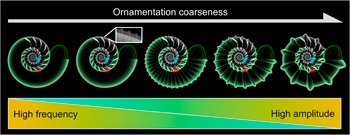


 Open access