1. Introduction

Ongoing glacier shrinkage in the European Alps is of increasing interest because of the expected changes in the hydrologic regime of major river catchments (e.g. Reference Mauser and BachMauser and Bach, 2009; Reference HussHuss, 2011) and its influence on hydro-power production (e.g. Reference Schaefli, Hingray and MusySchaefli and others, 2007; Reference Terrier, Jordan, Schleiss, Haeberli, Huggel, Kunzler, Schleiss and BoesTerrier and others, 2011; Reference Farinotti, Usselmann, Huss, Bauder and FunkFarinotti and others, 2012), tourism (Reference Fischer, Olefs and AbermannFischer and others, 2011) and natural hazards (e.g. Reference MooreMoore and others, 2009; Reference Frey, Haeberli, Linsbauer, Huggel and PaulFrey and others, 2010; Reference Haeberli, Clague, Huggel, Kaab, Ubeda, Vericat and RedsHaeberli and others, 2010; Reference Kunzler, Huggel, Linsbauer, Haeberli, Malet, Glade and CasagliKunzler and others, 2010). Scenarios of future climate change with further increasing temperatures (Reference SolomonSolomon and others, 2007) involve continued, if not accelerated, glacier shrinkage, and even the possibility of complete loss of glaciers in entire mountain ranges (e.g. Reference Zemp, Haeberli, Hoelzle and PaulZemp and others, 2006). Several methods, based on different basic concepts, complexity and application scales, have been developed to determine future glacier evolution (i.e. change in glacier area and/or volume) along with the related changes in runoff. Such glacier models can either be regionally calibrated empirical/statistical models or process-oriented models, which are more physically based (Reference Hoelzle, Paul, Gruber and FrauenfelderHoelzle and others, 2005).

For modelling glacier evolution at the scale of entire mountain ranges, a variety of simple techniques and approaches (requiring only few input data) have been applied in the past. Examples are a shift of the equilibrium-line altitude (ELA), according to given changes in temperature and/or precipitation and the related change of the accumulation area (e.g. Reference Lie, Dahl and NesjeLie and others, 2003; Reference Zemp, Haeberli, Hoelzle and PaulZemp and others, 2006; Reference Condom, Coudrain, Sicart and TheryCondom and others, 2007; Reference Paul, Maisch, Rothenbuhler, Hoelzle and HaeberliPaul and others, 2007), the application of various spatio-temporal extrapolation techniques (Reference HussHuss, 2012) or the parameterization scheme for glacier inventory data introduced by Reference Haeberli and HoelzleHaeberli and Hoelzle (1995). Using even more simplified methods, future glacier changes are also modelled at a global scale, for example to assess the future contribution of glaciers to sea-level rise, mostly as a combination of analogy concepts and multivariate analysis with strongly abstracted glaciers (e.g. Reference Raper and BraithwaiteRaper and Braithwaite, 2005; Reference Bahr, Dyurgerov and MeierBahr and others, 2009; Reference Marzeion, Hofer, Jarosch, Kaser and MolgMarzeion and others, 2012). Reference Radic = and HockRadic= and Hock (2011) and Reference Raper, Brown and BraithwaiteRaper and others (2000) considered the change in a standardized area/elevation distribution (hypsometry) to account for the adjustment of glacier area to future climate conditions. A more direct way to determine future glacier evolution is the calculation of glacier volume loss based on observed overall changes in glacier thickness, as derived from geodetic measurements (e.g. differencing of two digital elevation models (DEMs)) over a longer time period (e.g. Reference Huss, Jouvet, Farinotti and BauderHuss and others, 2010a). Based on these observations, simple parameterizations of thickness evolution can be derived and, in combination with calculated ice-thickness distributions (e.g. Reference Farinotti, Huss, Bauder and FunkFarinotti and others, 2009; Reference Linsbauer, Paul and HaeberliLinsbauer and others, 2012) and mass balances (e.g. Reference Giesen and OerlemansGiesen and Oerle-mans, 2012), be applied to large glacier samples (e.g. Reference HussHuss, 2011; Reference Salzmann, Machguth and LinsbauerSalzmann and others, 2012).

A variety of more complex approaches exist to model future glacier evolution, based on mass-balance modelling and glacier flow (e.g. Reference Le Meur, Gerbaux, Schafer and VincentLe Meur and others, 2007; Reference Jouvet, Huss, Blatter, Picasso and RappazJouvet and others, 2009, Reference Jouvet, Huss, Funk and Blatter2011). These models are computationally expensive and only applicable to individual well-studied glaciers, where sufficient data (also for calibration and validation) exist.

Ultimately, the glacier-evolution models described above must be linked to a climate scenario, and changes should be time-dependent. Although models that are based on mass-balance calculations can be directly linked to climate model output (e.g. Reference Machguth, Paul, Kotlarski and HoelzleMachguth and others, 2009), the modelled mass change is not identical to thickness change, as the geometric adjustment of a glacier (change in area or length) to a mass-balance forcing will only occur after a delay. Using a (surface) mass-balance model to determine future glacier evolution has thus to implement a parameterization of mass transport. This can be obtained by a comparison of the modelled cumulative mass budget and the observed overall volume loss over the same period (Reference Huss, Jouvet, Farinotti and BauderHuss and others, 2010a). For the simpler approaches (e.g. shift in the ELA) the link to a certain climate scenario can be established, based on atmospheric lapse rates or known relations between ELA change and changes in temperature, precipitation and the energy balance (e.g. Reference KuhnKuhn, 1981). However, the involved time dependence of the geometric adjustment has to be introduced artificially, for example based on estimated response times for larger glacier samples (e.g. Reference Haeberli and HoelzleHaeberli and Hoelzle, 1995).

Although the various existing approaches have structurally different designs and use different climate forcings, they tend to provide similar results. A model intercomparison can help to tease out model-specific problems and hence sources of uncertainty for simulations and predictions. Thereby, the boundary conditions for the compared approaches are usually held constant and the models compared are conceptually rather similar. Models that use conceptually different approaches have not, so far, been analysed together. Here we compare three methods of variable complexity applicable to large glacier populations and focus on the glaciers of the Swiss Alps.

Besides comparing the modelled glacier extents, hypsometric distributions and relative area loss for M1, M2 and M3, we also analysed the uncertainties introduced by model simplifications, the ice-thickness estimations and the climate change scenarios. Because future glacier extents or runoff from glacierized catchments cannot be validated, a validation can only be performed over the recent past. We thus compared the modelled area and/or volume changes over the 1985-2000 period with the observed ones, being well aware that none of the three models are designed to give reliable results over such a short timescale.

2. Study Region and Input Ata

The study region of the Swiss Alps comprises an area of ∼25 000 km2 including a glacierized area of ∼1300 km2 in 1973 (Reference Muller, Caflisch and MullerMuller and others, 1976) (Fig. 1). The DEM covering the study site was produced by the Swiss Federal Office of Topography (swisstopo), has a cell size of 25m (termed DEM25 in the following) and approximately represents the glacier surfaces around 1985 (Reference RickenbacherRickenbacher, 1998; swisstopo, 2005). The accuracy of the DEM25 is reported to be 2.5-7.5 m in the horizontal direction and <10m in the vertical direction (swisstopo, 2005). The digital glacier outlines are based on the digitized Swiss Glacier Inventory from 1973 (SGI1973) by Reference Muller, Caflisch and MullerMuller and others (1976), in the revised version by Reference Maisch, Wipf, Denneler, Battaglia and BenzMaisch and others (2000) which includes 2365 glacier and glacierets >0.01 km2 . These glacier polygons fit well to the glacier extent in the DEM25, as only small overall area changes took place for most glaciers in the Alps between 1973 and 1985 (Reference Paul, Kaab, Maisch, Kellenberger and HaeberliPaul and others, 2004). While the first two models (M1 and M2) were applied to all glaciers in the Swiss Alps, M3 was restricted to a sample of 101 selected glaciers, as explained in Section 3.3, representing ∼ 5 0% of the total glacierized area and ∼ 7 5% of the ice volume in Switzerland.

Fig. 1. The model domain ‘Swiss Alps’ with the subsample of 101 selected glaciers marked. The white points denote the locations of the MeteoSwiss weather stations with homogenized annual mean temperature data for the period 1980–2009. ALT: Altdorf (438ma.s.l.), CHD: Chateau-d’Oex (985ma.s.l.), CHU: Chur (556ma.s.l.), DAV: Davos (1594ma.s.l.), ENG: Engelberg (1035ma.s.l.), GRH: Grimsel Hospiz (1980 m a.s.l.), GSB: Col du Grand St Bernhard (2472 m a.s.l.), JUN: Jungfraujoch (3580m a.s.l.), OTL: Locarno/Monti (366m a.s.l.), SAE: Santis (2502 m a.s.l.), SAM: Samedan (1708m a.s.l.), SBE: S. Bernardino (1638 m a.s.l.) and SIO: Sion (482m a.s.l.). Black rectangles show the extent for Figures 4 and 7.

The ice-thickness distribution for all Swiss glaciers is calculated with the GlabTop model (Reference Linsbauer, Paul and HaeberliLinsbauer and others, 2012; Reference Paul and LinsbauerPaul and Linsbauer, 2012) using the DEM25 and the glacier outlines from the SGI1973 as inputs. GlabTop spatially extrapolates locally (50 m elevation bins) estimated glacier thickness values that are derived from averaged values of surface slope and a mean basal shear stress per glacier (assuming perfect plasticity; see Reference PatersonPaterson, 1994). The basal shear stress was empirically derived from the glacier elevation range, which can be seen as a proxy for mass turnover (Reference Haeberli and HoelzleHaeberli and Hoelzle, 1995), and has an upper-bound value of 150 kPa for glaciers exceeding an elevation range of 1.6 km (Reference Li, Ng, Li, Qin and ChengLi and others, 2012). The obtained model results have an uncertainty range of about ±30%, as shown by a comparison with independent radar profiles and an uncertainty analysis (Reference Linsbauer, Paul and HaeberliLinsbauer and others, 2012).

The presence of glaciers, their number and characteristics are mainly linked to the elevation of their headwater catchment, which determines the seasonality of the runoff regime (mostly pluvio-nival or glacio-nival). Most Swiss glaciers (exceptions are found in the Val Bregaglia and the Val Fenga) are drained by seven major river catchments with gauging stations in the lowlands. In combination with the outlines of these major river catchments, the grid from the DEM differencing (Shuttle Radar Topography Mission DEM (SRTM3)-DEM25) by Reference Paul and HaeberliPaul and Haeberli (2008) was used to obtain catchment-specific elevation changes over the period 1985-99, based on zone statistics (with each major river catchment as a zone). Apart from a few regions with data voids over glaciers, this dataset covers nearly all glaciers in the Swiss Alps. The mean change of the DEM differencing (—11 mw.e.) is in good agreement with the mean cumulative mass budget of nine Alpine glaciers with measured mass balances (—10.8m w.e.).

Both the reported temperature data from Reference Rebetez and ReinhardRebetez and Reinhard (2008) and the measured temperatures from 13 selected weather stations (Fig. 2) run by the Swiss Federal Office of Meteorology and Climatology (MeteoSwiss) show a distinct temperature increase of ∼1°C between 1980 and 1995. From the 1990s until the present the temperatures further increased (by ∼0.5°C), but at a lower rate (Fig. 2).

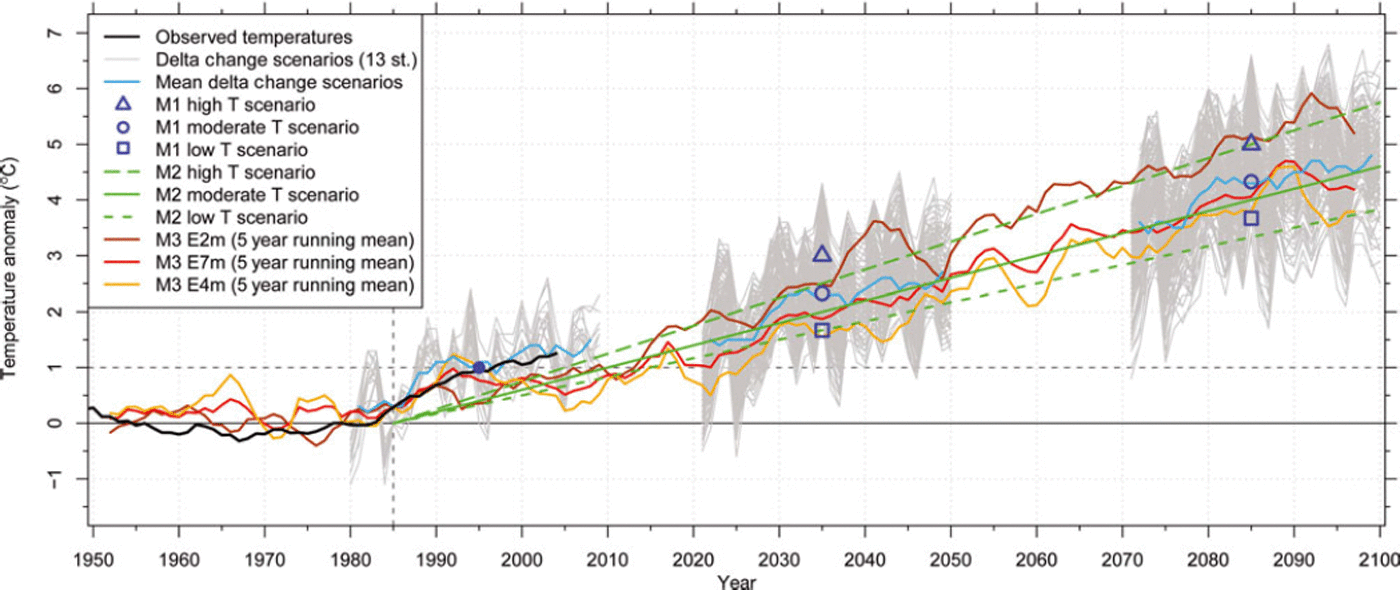
Fig. 2. Anomaly of 2m air temperature of the observed temperatures and climate scenarios used, all normalized to the reference period from 1961–90 for Switzerland (after Reference Rebetez and ReinhardRebetez and Reinhard, 2008). As a reference, the annual temperature anomalies (Reference Rebetez and ReinhardRebetez and Reinhard, 2008) from 12 homogenized temperature series for 12 stations in Switzerland (Reference Begert, Schlegel and KirchhoferBegert and others, 2005) are displayed in black. The grey lines show observed temperatures from 13 MeteoSwiss weather stations (Fig. 1) for the control period 1980–2009 and their projections to the two scenario periods 2021–50 and 2070–99 according to the delta change values and ten different model chains from Reference Bosshard, Kotlarski, Ewen and ScharBosshard and others (2011). In light blue the 5 year running mean for the measurements and the projections for the 13 weather stations are shown. The blue point is the starting point for all three M 1 scenarios, and the triangle, circle and square mark the low-, moderate- and high-temperature scenarios for M1. The lines of the linear extrapolated temperature trends, as used for M2, are shown in green. The 5 year running mean for three scenario ensembles (E2m, E7m and E4m) used for M3 are shown in in orange, red and brown.

The three climate scenarios applied here are derived from ten climate model chains (combination of a general circulation model (GCM) and an RCM) using an A1B emission scenario (Reference SolomonSolomon and others, 2007) at a 25 km horizontal resolution from the EU-ENSEMBLES program (Reference Van der Linden and MitchellVan der Linden and Mitchell, 2009). Values for temperature and precipitation for several MeteoSwiss weather stations were downscaled for the scenario periods 2021-50 and 2070-99 (relative to the control period 1980-2009) by Reference Bosshard, Kotlarski, Ewen and ScharBosshard and others (2011) using a delta change approach. From the resulting temperature increase at 13 weather stations we derived low, moderate and high scenarios, that cover the range of model chain variability. The moderate scenario gives an increase in air temperature of 2°C and 4°C for the two scenario periods centred around 2035 and 2085, respectively.

Glacier development until the first scenario period in model M1 is based on the reaction to the 1°C temperature increase that took place in the 1980s. After that, glaciers react to the three scenarios of temperature increase derived for the first scenario period. The three scenarios for model M2 follow three linear trend extrapolations, assuming that the above-mentioned temperature increase of 1°C is repeated every 20, 25 or 30 years. The 25 year repeat period (i.e. the moderate scenario) also gives a 2°C and 4°C temperature increase by 2035 and 2085 (Fig. 2). The distributed mass-balance model applied in M3 is directly forced with three ensemble means of the A1B scenario using RCM simulations from ENSEMBLES, assuming ensemble means are the most plausible scenario guess (e.g. Reference Guo, Dirmeyer, Gao and ZhaoGuo and others, 2007). Ensemble E7m consists of seven different RCM realizations (driven by ECHAM5-r3, HadCM3Q0 and the ARPEGE GCMs), E4m consists of four RCMs all driven with ECHAM5-r3 and E2m is the ensemble of the two HadCM3Q0-driven ensembles (Reference Salzmann, Machguth and LinsbauerSalzmann and others, 2012). Monthly resolution RCM grids were chosen because the daily resolution grids showed unrealistic variability in daily precipitation.

The climate model input datasets are thus different by source, but not by value (Fig. 2). The moderate scenarios from M1 and M2, as well as E7m from M3 (the moderate scenario used in this model), all project a 2°C temperature increase for the two scenario periods centred around 2035 and 2085.

3. Methods

For all three models, the initial glacier extent is given by the glacier outlines from 1973 (SGI1973; Reference Maisch, Wipf, Denneler, Battaglia and BenzMaisch and others, 2000) and the swisstopo DEM25 with 25 m resolution, referring to the glacier surfaces at around 1985. The starting point 1973/1985 was chosen as most glaciers were close to a dynamic steady state then. The required ice-thickness distribution for models M2 and M3 is taken from Reference Linsbauer, Paul and HaeberliLinsbauer and others (2012).

3.2. Thickness change parameterization (M2)

Since the beginning of the 1980s, increasingly negative glacier mass balances have been observed in the Alps (Reference Zemp, Nussbaumer, Gartner-Roer, Hoelzle, Paul and HaeberliWGMS, 2011). The related thickness change for the period 1985-99 was calculated for all Swiss glaciers from DEM differencing (Reference Paul and HaeberliPaul and Haeberli, 2008), revealing strong thickness losses for low-lying and flat glacier tongues. This illustrates that the adaptation of the glacier extent to a rapidly changing climate can be dominated by thickness loss (downwasting) rather than area change (Reference Huss, Farinotti, Bauder and FunkHuss and others, 2008, Reference Huss, Jouvet, Farinotti and Bauder2010a). Plotting thickness loss vs altitude for the major river catchments reveals a rather similar and increasing thickness loss towards lower elevations for all regions (Fig. 3). To parameterize this for the entire study region, we used (similarly to Reference Huss, Jouvet, Farinotti and BauderHuss and others, 2010a) an empirically derived elevation-dependent function as an average for catchment-related mean values composed of a lower (<2000m) linear decline and an upper (>2000 m) quadratic decrease:

(1)

Fig. 3. Thickness changes from 1985 to 1999 (Reference Paul and HaeberliPaul and Haeberli, 2008) for seven major river catchments, together with an empirical elevation-dependent function to parameterize the thickness loss for all Swiss glaciers in model M2 (Eqn (1)).

with dh/dt the rate of thickness change (ma-1) within the specified time period and DEMi the elevation (ma.s.l.) of each gridcell. Of course, the assumption that all glaciers are subject to the same elevation-dependent thinning rates is not correct (e.g. delay due to debris cover or different shading conditions) and the resulting area changes can be strongly over- or underestimated for individual glaciers. Above 3000 m the approximation of the parameterization differs from the extracted thickness loss rates in Figure 3, but values in this elevation range are influenced by artefacts in the SRTM3 DEM. The decrease to zero at the highest elevations is implemented to keep small, steep and thus thin glaciers at high elevations from disappearing too fast. The function used is an empirical one, rather than derived by a regression, to better accommodate the DEM uncertainties and model needs mentioned above. In this regard it has to be stressed that the modelled area changes are assumed to be realistic only at the regional scale (e.g. for major river catchments).

M2 is coupled with climate by (1) relating the observed thickness change from 1985 to 1999 to the observed temperature increase of 18C mentioned above and (2) assuming that the glacier surface will adjust to this forcing over a 20, 25 or 30 year time period (Fig. 2). This trend is then assumed to continue into the future (linear extrapolation), resulting in a 18C temperature increase every 20, 25 and 30 years. Glacier area is removed once the cumulative ice-thickness loss exceeds the initial ice thickness. Each time the thickness change increment is subtracted from the initial DEM, the glacier surface gradually shifts to lower elevations, where the rate of thickness loss is higher.

3.3. Glacier mass-balance simulation and retreat modelling for 101 glaciers (M3)

Glacier mass balance is calculated using a distributed mass-balance model (Reference Machguth, Paul, Kotlarski and HoelzleMachguth and others, 2009). This is a simplified energy-balance model, which runs at daily time-steps and uses gridded RCM data of 2 m air temperature, T, precipitation, P, and total cloudiness, n, for input. Because of spurious values in the daily RCM fields, the data applied here are at monthly resolution. Daily values are generated from linear interpolation, and precipitation falls every fifth day (Reference Salzmann, Machguth and LinsbauerSalzmann and others, 2012). Cumulative mass balance, bc, on day t + 1 is calculated for every time-step and over each gridcell of the DEM, according to Reference OerlemansOerlemans (2001):

(2)

where t is the discrete time variable, Δt is the time-step, lm is the latent heat of fusion of ice (334 kJ kg∼1) and Psolid is solid precipitation (m w.e.). The energy available for melt, Qm, is calculated as

(3)

where a is the surface albedo (three constant albedo values are applied: snow = 0.72, firn = 0.45 and ice = 0.27), Sin is the incoming shortwave radiation at the surface, calculated according to Reference Greuell, Knap and SmeetsGreuell and others (1997) from n and clear-sky global radiation computed at DEM resolution and taking all effects of exposition and shading into account, T is in 8C, and C0 + C 1T is the sum of the longwave radiation balance and the turbulent exchange (Reference OerlemansOerlemans, 2001). C1 is set to 12 W mr2 K∼1 and C0 is tuned to —45 W mr2 (Reference Machguth, Paul, Kotlarski and HoelzleMachguth and others, 2009). Accumulation is equal to Psolid, the redistribution of snow is not taken into account and a threshold range of 1-28C is used to distinguish between snowfall and rain. Any meltwater is considered as runoff, i.e. refreezing and internal storage of meltwater is neglected.

Glacier retreat is simulated based on the modelled mass balances and the so-called Δh glacier-retreat approach, following Reference Huss, Jouvet, Farinotti and BauderHuss and others (2010a). The latter parameterize glacier surface elevation change by distributing glacier mass loss or mass gain over the entire glacier surface, according to altitude-dependent functions of observed changes in glacier thickness. Here we use the glacier-size-dependent Δh functions as proposed for the Swiss Alps (Reference Huss, Jouvet, Farinotti and BauderHuss and others, 2010a, fig. 3b therein). Glacier geometry is updated annually, based on calculated surface elevation changes. Glacier surface mass balance is calculated on the updated topography and thus considers the mass-balance/altitude feedback, i.e. a reduction in glacier thickness results in a lower elevation of the glacier surface and consequently a more negative mass balance (e.g. Reference Raymond, Neumann, Rignot, Echelmeyer, Rivera and CasassaRaymond and others, 2005). Glacierized gridcells become ice-free when their elevation falls below the elevation of the glacier bed.

Simplifications in the mass-balance model used (e.g. debris cover is not considered) limit the number of glaciers where reasonable mass balances can be calculated. Therefore, 101 glaciers are selected from the SGI1973, based on the following criteria: (1) no or little debris cover; (2) no or little influence of avalanches; (3) mass loss restricted to melting (the applied mass-balance model does not consider any processes like calving into lakes or over rock faces); and (4) sufficient size (>1 km2), as small glaciers usually show accumulation patterns of a very local nature with strong influence from wind-drift and avalanching.

M3 is coupled to climate using gridded RCM fields for model input, rather than projected temperature change at weather station locations (cf. models M1 and M2). The direct use of the RCM fields involves the two steps of (1) downscaling the gridded 25 km resolution fields to the 100 m resolution of the mass-balance model, and (2) de-biasing the downscaled RCM fields. These two steps are implemented in the mass-balance modelling set-up and directly applied to each RCM grid while the model is running. The downscaling of T and P is based on interpolation of the RCM values with the subsequent application of simple subgrid parameterizations, while Sin is computed from high-resolution clear-sky global radiation and attenuation from clouds derived from interpolated total cloudiness, n (see Reference Machguth, Haeberli and PaulMachguth and others, 2012, for full details).

The de-biasing of the RCM fields is done for each variable, according to the method described by Reference Machguth, Haeberli and PaulMachguth and others (2012), where biases in RCM values of T and n are established from comparison with observations at 14 high-mountain weather stations in the Swiss Alps and spatial distribution of RCM precipitation is scaled to match the precipitation pattern of the Reference Schwarb, Daly, Frei and ScharSchwarb and others (2001) precipitation map. However, the accuracy of the downscaled and de-biased fields is limited, as knowledge of real meteorological conditions at the glacier sites is imperfect. In particular, the large uncertainties in observed high-mountain precipitation (Reference SevrukSevruk, 1997) hamper the de-biasing procedure and make it impossible to achieve a level of accuracy that would allow the calculation of accurate mass balances for each individual glacier. This issue is reflected in the successful model-calibration to observed melt during the summer period while at the same time winter mass balance strongly disagrees with measurements (Reference Machguth, Paul, Kotlarski and HoelzleMachguth and others, 2009). We have approached these limitations by applying a calibration procedure, where the mass-balance model is driven by the downscaled and de-biased RCM time series for the period 1970-2000 and precipitation is adjusted for each glacier individually to achieve a prescribed cumulative mass balance (Reference Machguth, Haeberli and PaulMachguth and others, 2012). Choosing an appropriate value for the cumulative mass balance is challenging, as available observations differ: while Reference Zemp, Paul, Hoelzle, Haeberli, Orlove, Wiegandt and LuckmanZemp and others (2008) report a mean cumulative mass balance of — 13mw.e. for nine Alpine glaciers, Reference Huss, Hock, Bauder and FunkHuss and others (2010b,Reference Huss, Usselmann, Farinotti and Bauderc) calculate —9mw.e. from a combined approach of modelling and observations. We prescribe a cumulative mass balance of — 11mw.e., which is midway between the two values. Furthermore, all glaciers were calibrated to the same cumulative mass balance. This simplification had to be introduced because, for most of the 101 selected glaciers, no individual observational records are available. We are confident that the latter simplification only marginally affects the calculated future glacier volumes. Reference Salzmann, Machguth and LinsbauerSalzmann and others (2012) applied the same model chain and showed that using alternative sets of non-uniform cumulative mass balances in the calibration procedure has a negligible impact on future scenarios. The downscaled, de-biased and calibrated RCM data are subsequently used to run the mass-balance model over the entire scenario period.

4. Results

The simulated glacier area loss for all three models is illustrated in Figure 4. For M1 the moderate scenario is displayed, with an ELA shift of 150 m until the first scenario period and a shift of another 200 m until the second scenario period. As this model is a two-dimensional simplification of a glacier, it is limited to providing area changes (on the initial unchanged DEM) with the lower ends of the glaciers simply cut off. This leads to glacier geometries with cropped ablation and unchanged accumulation areas. The visual comparison with the moderate M2 and the M3 E7m scenario is provided nevertheless.

Fig. 4. Visualization of the results for the regions around Aletsch (a–c) and Rhone (d–f) glaciers for all three models (M1: (c) and (f); M2: (a) and (d); M3: (b) and (e)) with their moderate climate scenario, starting with their 1973 extent (i.e. DEM25). The colour steps depict 10year changes and are the same for all models. The modelling with M3 was restricted to the subsample of 101 glaciers.

Models M2 and M3 additionally require the ice-thickness distribution to calculate ice volume change, as a combination of surface lowering and area reduction. The resulting patterns of glacier shrinkage seem to be closer to reality than for M1, where for some glaciers the shrinkage starts along the edges (where the ice is thin) at the lowest elevations (where thinning is greatest). The visual comparison of M2 and M3 in Figure 4 and the quantitative comparison in Figure 6d indicate that the area loss in M3 is slightly faster than for M2.

The evolution of the area/elevation distribution (hyp-sometry) for 10year time-steps and the three moderate climate scenarios is depicted in Figure 5. While for model M1 the entire distribution, including the maximum value, is shifted upwards, model M2 shows a constant decrease at all elevations without a trend in the maximum. This is due to the implemented elevation feedback, i.e. large parts of the surface area shift to lower elevations (where melting is higher). Focusing on just the 101 selected glaciers from M3 using the other two models (Fig. 5, lower panels), the trends of the area distribution for M1 and M2 are the same as for the full sample. Interestingly, the hypsometric changes of M3 are rather similar to M1, but with an overall stronger loss in area at higher elevations and a reduced loss at lower elevations. In contrast to M1 and M2 which work at 25 m resolution, M3 operates at 100m resolution. Therefore, the initial glacier areas in Figure 5c and d and Figure 5e are not exactly the same.

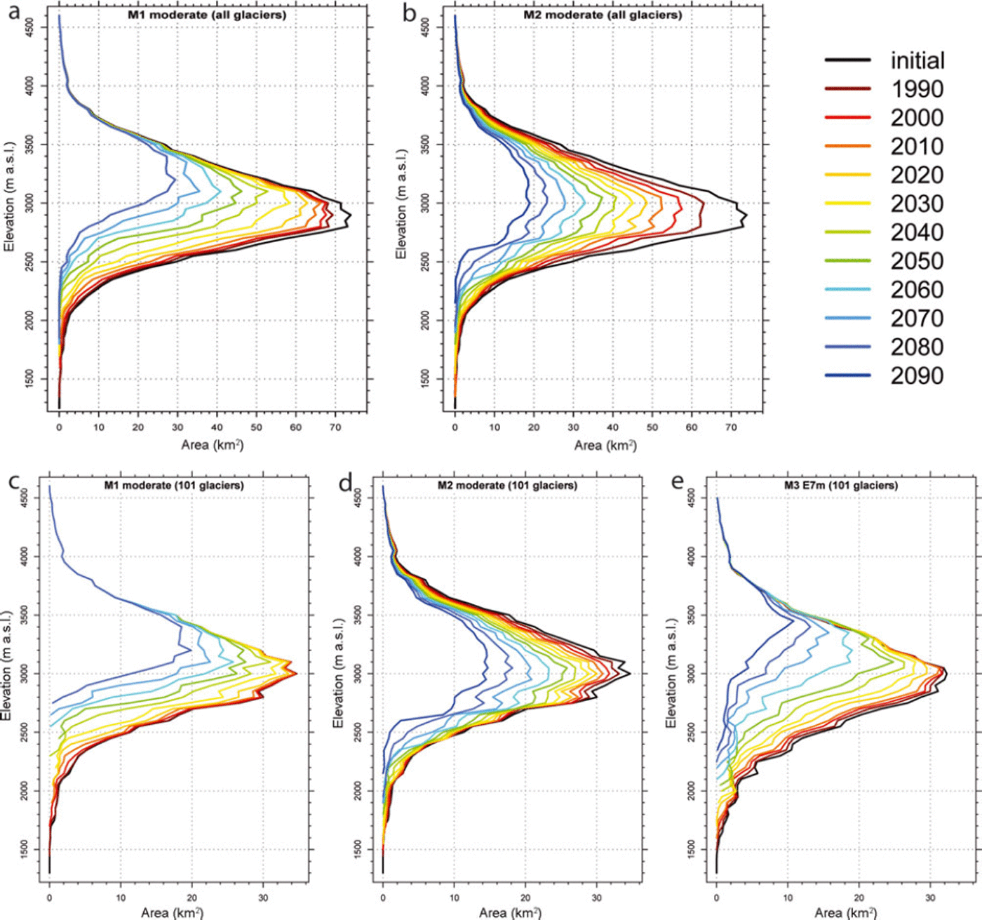
Fig. 5. Change in overall glacier hypsometry in 10 year steps (colour code is the same as in Fig. 4) until 2090 (2080 for M1) for all glaciers (a, b) and the 101 selected glaciers (c–e), calculated with the moderate temperature scenarios of M1 (a, c) and M2 (b, d) and ensembles scenario E7m from M3 (e).

Figure 6a-d show the temporal development of the area loss (and volume loss for M3) during the 21st century for all three models and their different realizations, corresponding to the different applied climate scenarios, the thickness uncertainty (M2) and the full sample vs the 101 selected glaciers (M1, M2). The development of the relative area change along the various model pathways is, to a large extent, similar, but differences are also visible. There is a spread of ∼10-20% around the near future (2035) and of ∼30-50% at the end of the century for the various model realizations in all four plots. Considering the simulations for the sample of the selected 101 glaciers, the general trend for all model realizations is the same: by mid-century the area loss is still moderate, but it then increases sharply until the end of the century, especially with M3 and the high-temperature scenarios of M1. This is also reflected in the glacier hypsometry modelled by M3 (Fig. 5e), which shows a marked increase in hypsometric area loss in the second half of the model simulation.

Fig. 6. Development of relative area loss from the model starting point (1985 for M1 and M2; 1970 for M3) until 2100 for all three models and their different realizations (scenarios, thickness, glacier samples). (a) The three retrospective applied scenarios for M1 represented by the grey lines for all glaciers and in black (bold) for the 101 glaciers. (b) The three different temperature trend extrapolations applied in M2 together with the corresponding ±30% uncertainty due to the ice-thickness modelling for all Swiss glaciers. (c) Area and volume loss for the selected 101 glaciers as modelled with the three climate scenario ensembles used in M3. (d) A comparison based on the sample of the selected 101 glaciers of the climate scenario runs from all three models.

In Figure 6a the curves for the applied climate scenario realizations for M1 (Section 3.1), with a first ELA shift of 150 m until the first scenario period and a further ELA shift of 100, 200 and 300 m after the first scenario period, are shown (for all glaciers and the 101 glaciers) leading to a spread of the modelled glacier area of 40% at the end of the century (loss of 55-95% by 2100). There is no large difference between the curves for all glaciers and those for the 101 glaciers.

The 30% uncertainty in the glacier thickness (Fig. 6b) results in a spread of not more than 20%, considering area loss as modelled with M2 for the three climate scenarios. The spread of the lines reproducing area loss according to the three different scenarios is much larger (∼40% around the second scenario period), whereby the high-temperature scenario (+5.758C temperature increase by 2100) results in an almost complete loss of glaciers (∼90%). The uncertainty in ice thickness (±30%) has a nonlinear impact on glacier retreat. With 30% thinner ice the extent of the reference thickness is reached 20 years earlier, while 30% thicker ice gives only 10 additional years before this extent is reached. Thus, differences in ice-thickness estimations directly impact the timescales of the scenarios, but might have a smaller effect on the remaining ice in 2100 than that resulting from the uncertainties in temperature change (Fig. 6b and d).

In Figure 6c the evolution of area and volume for the selected 101 glaciers as modelled with three scenario ensembles and with M3 is shown. The behaviour of the curves is rather similar, differing only in the speed of area loss, resulting in a spread of ∼20% at the second scenario period.

For the comparison in Figure 6d, all scenario runs for all three models for the 101 selected glaciers are displayed. It shows that the uncertainties introduced by different realizations of climate change are very similar during the first scenario period and rather large in the second scenario period. Thus, model results increasingly deviate when going into the future. The moderate scenarios of the three models (M1 mod., M2 mod. and M3 E7m) result in a total loss of glacier area of ∼60-80% by around the year 2100. In terms of area loss, the scenarios M1 mod., M2 high, M3 E4m and M3 E7m are close together, i.e. they do not differ by more than 15%. The area loss modelled by scenarios M1 low, M2 mod. and, in particular, M2 low is rather slow compared to the other scenarios and can be seen as a lower boundary.

The variable curvature of the lines reveals interesting details about the speed of glacier shrinkage at various phases of the recession, largely depending on the remaining area covered by thick ice. A key aspect is that all curves will finally approach 0, i.e. glaciers are unable to stabilize their extent for the given scenarios of climate change. This behaviour is also visible in the hypsometric changes in Figure 5b, where the area loss (all glaciers) is relatively large between the initial and the first step, whereas in Figure 5d there is not much difference between these two curves.

In contrast to M1 and M2, which have a fixed starting point in 1985, the model start of M3 is 1970. This is done to maximize the length of the calibration period. For the model comparison the earlier starting point of M3 is of negligible importance, as the climate was approximately stable and, according to M3, only 2.5% (15 km2) of the area and 5% (2.8 km3) of the initial volume were lost between 1970 and 1985.

5. Validation

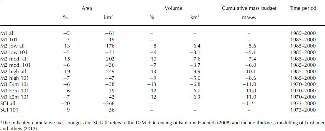
For M3 (and all three ensemble scenarios) the cumulative mass balance for the time period 1970-2000 is calibrated to an overall mass loss of —11 m w.e., the mean calculated from the observed cumulative mass budget of Reference Zemp, Paul, Hoelzle, Haeberli, Orlove, Wiegandt and LuckmanZemp and others (2008) (—13 m w.e.) and Reference Huss, Hock, Bauder and FunkHuss and others (2010b,Reference Huss, Usselmann, Farinotti and Bauderc) (—9 m w.e.) (Reference Salzmann, Machguth and LinsbauerSalzmann and others, 2012). Within this calibration period, a model validation for M1, M2 and M3 would be possible, as corresponding and consistent glacier outlines for nearly all Swiss glaciers exist for 1973 and 2000 (SGI2000; Reference Paul Paul, 2007). In Table 1 the area (and where available the volume) of all model scenarios and the glacier inventories is displayed to allow comparison in a quantitative manner. The observed area loss is 2 0% for all glaciers and 9% for the 101 glaciers. The M3 scenarios and the moderate and high M2 scenarios do not differ by more than 5% from these values. The cumulative mass budgets for the M3 scenarios are calibrated, but the value obtained for the high M2 scenario for all glaciers corresponds rather well to the observations (Reference Paul and HaeberliPaul and Haeberli, 2008). Cumulative mass budget for the moderate M2 scenario is within the range of values of Reference Huss, Hock, Bauder and FunkHuss and others (2010b, Reference Huss, Usselmann, Farinotti and Bauderc). Area (and volume) losses for M1 and the low M2 scenario are probably too low. This is expected for M1, where only the lowermost parts of the glaciers were removed, according to an AAR0 of 60%. As many of the lower parts of the larger glaciers in 1973 ended in narrow tongues, only minor parts of the area are deleted.

Table 1. Comparison of area and volume loss and cumulative mass budgets for all scenarios of M1, M2 and M3 from their model start until the validation year 2000, together with the derived area loss obtained by comparing the two relevant Swiss Glacier Inventories (SGI) from 1973 and 2000. Results are tabulated for all Swiss glaciers and for the subset of 101 glaciers

In Figure 7 a comparison of observed and modelled glacier extents for the year 2000 is shown for the glaciers in the Bernina region. It has to be kept in mind that M1 and M2 are designed to model glacier evolution on a regional scale, rather than individual glaciers, and that only three time-steps are applied until 2000. As can be seen, the changes in the observed glacier extents (1973–2000) for the large glaciers occur at the snout and along the edges. Some glaciers show a distinct retreat of the tongue from 1973 to 2000, but in general all glaciers lost area all over their margins due to the implemented surface lowering.

Fig. 7. The extents of glaciers in the Bernina region according to the inventories from 1973 and 2000 and the modelled ice thickness for the year 2000 according to Reference Linsbauer, Paul and HaeberliLinsbauer and others (2012), compared to the modelled area evolution with the moderate scenarios of M1, M2 and M3 for the time-step corresponding to the year 2000. The inset shows the Tschierva glacier snout with all the glacier margins according to all model scenarios.

For the glaciers depicted in Figure 7, both M2 and M3 reproduce well the observed inward shift of glacier boundaries due to surface lowering. The agreement between observed and modelled terminus positions of Tremoggia, Tschierva and Morteratsch glaciers is good, while the modelled retreat for Palu = and, especially, Roseg glaciers is too small (Fig. 7). Generally, the area and in particular the volume loss as modelled with M3 is larger than with M2, as mentioned above (Figs 4–6). This is also illustrated in the inset map of Figure 7. It shows the tongue of Tschierva glacier with outlines for the year 2000 as modelled by all models (and scenarios). M1 shows the typical pattern resulting from cutting off the lowermost part of the tongue, with a retreat of about 200m compared to the mapped glacier outline, while the other two models achieve a glacier outline similar to the mapped tongue position.

6. Discussion

6.2. Possibilities and limitations of model applications

For a sound model intercomparison, the models can only be compared against observed changes in the past. As the model starting point is 1985 for M1 and M2 and 1970 for M3, there is only a short time period available for a comparison. This comparison might not really be seen as a validation, as none of the models are expected to provide useful results over this timescale. However, for the year 2000, modelled glacier extents fit the mapped ones rather well. As the modelled future changes are much larger than the changes observed over this 15 year period, the significance of this comparison is limited.

The modelled area losses (Fig. 6) clearly reflect the temperature trends of the applied climate scenarios (Fig. 2). The three moderate scenarios that prescribe a 2°C or 4°C temperature increase for the two scenario periods centred around 2035 and 2085 show a comparable area loss over time (with a maximal spread of ∼20%). The spread in area loss of ∼ 5 0% by 2100 is given by the low-temperature scenario of M2 (upper boundary) and the E2m scenario of M3 (lower boundary).

M1 and M2 are highly simplified models, but provide glacier change scenarios for large glacier samples at a regional scale with a small computational effort. This is in contrast to M3, that better considers characteristics of individual glaciers. Though the simplifications in M1 and M2 are substantial, they might be considered as being compliant with the uncertainties of the RCM scenarios, i.e. the variability in area change introduced by the simplifications is of the same order of magnitude as that resulting from the unknown future climate. According to the results of this comparison, the latter is somewhat larger. For studies seeking to establish future trends in the glacier cover of entire mountain ranges (e.g. the Swiss Alps), M1 and M2 are fast approaches providing results similar to the more detailed modelling of M3. As both models apply average parameter sets to all Swiss glaciers, the results are valid on the sample as a whole. We also found agreement with results from completely different studies (Reference Jouvet, Huss, Blatter, Picasso and RappazJouvet and others, 2009, Reference Jouvet, Huss, Funk and Blatter2011; Reference Huss, Jouvet, Farinotti and BauderHuss and others, 2010a; Reference HussHuss, 2012), which is not surprising as the strong future temperature increase dominates the response. The simple approach of M1 was designed to provide adjusted glacier areas as an input for hydrological models operating at a regional scale (e.g. Reference Viviroli, Zappa, Gurtz and WeingartnerViviroli and others, 2009; Reference Koplin, Schadler, Viviroli and WeingartnerKoplin and others, 2012). This study has shown that area loss is fastest in M1, which can be seen as a lower-bound timescale for the expected terminus retreat. For the hydrological model that generates additional runoff solely from the change in glacier area, the stronger area change in M1 might be well suited to mimic the expected future increase in runoff due to downwasting, a process that is not included in M1 but important in reality.

Although all three models are based on equivalent climate scenarios and RCM runs, the coupling to the climate model output is rather different: retrospective with M1; based on trend extrapolation with M2; and directly driven by RCM grids in M3. The modelled future development in glacier extent with the moderate scenarios can already be seen as lower-bound estimates, as the current temperature increase is already stronger and modelled mean annual thickness loss from 2000 to 2010 (with M2 mod. and M3 E7m; Fig. 8) is only 0.4 ma∼1 according to the models, instead of the observed 0.8 m a∼1 (Reference Zemp, Hoelzle and HaeberliZemp and others, 2009). The decrease in mean annual thickness change in the last part of the modelling period for all scenarios in M3 (Fig. 8) may be related to the direct coupling with RCM data (allowing for positive and negative mass balances) and a possible future adjustment of the remaining small glaciers at high elevation.

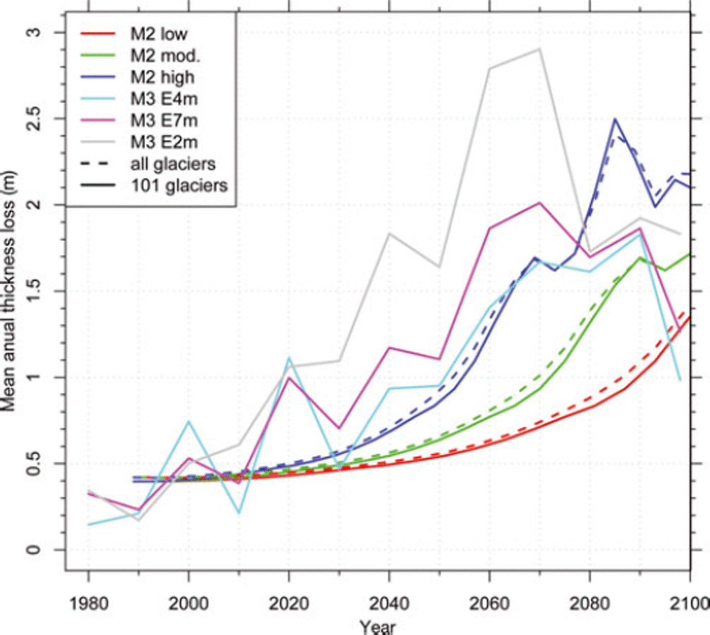
Fig. 8. Mean annual thickness loss over time, as derived from the three scenarios of M2 and the three ensemble means of M3.

Finally, it has to be considered that several feedbacks are not incorporated in any of the models, including the change of albedo (Oerlemans and others, 2009), development of new lakes (Reference Frey, Haeberli, Linsbauer, Huggel and PaulFrey and others, 2010), increasing debris cover (Reference Jouvet, Huss, Funk and BlatterJouvet and others, 2011) and changes in glacier thermal state (Reference Vincent, Le Meur, Six, Possenti, Lefebvre and FunkVincent and others, 2007; Reference Hoelzle, Darms, Luthi and SuterHoelzle and others, 2011). The local and general influence of these processes is difficult to assess because they partly act in opposite directions.

7. Conclusion

The three compared approaches for calculating future glacier evolution use robust (based on simple physical laws or observations) but simplified parameterizations that are applicable to large glacier samples. Two of the models are implemented in a GIS processing environment and enable glacier change scenarios to be simulated at a regional scale with small computational costs. From the comparison of the three models we conclude the following:

All three models have advantages and disadvantages in their application. Which model to choose for a specific application depends on data availability and the level of detail required in the output. M1 and M2 have proven to provide fast and robust first-order estimates for glacier retreat, dominated by temperature increase. They might be less suitable when changes in precipitation have to be considered as well, but here the uncertainties are even larger.