

Introduction
During the 1980s and 1990s, several investigators proposed that climate warming would increase snowfall to Antarctica. Increased water storage within the ice sheet would then mitigate sea-level rise (e.g. Reference Connolley and KingConnolley and King, 1993; Reference ThomasThompson and Pollard, 1997; Reference Wang, Wen and LiuWen, 1998). However, recent studies show that flow speed has increased for some Antarctic outlet glaciers, resulting in increased mass losses from the ice sheet independent of changes in surface accumulation rate (e.g. Reference Liu, Jezek and LiPayne and others, 2004; Reference RignotShepherd and others, 2004; Reference SolomonThomas and others, 2004; Reference Wang, Wen, Liu, Jezek and CsathóWang and others, 2006b). The increased discharge has likely contributed to sea-level rise over the last decade (Reference Shepherd, Wingham and RignotSolomon and others, 2007). In this paper, we assess the mass budget of grounded ice in the Lambert Glacier–Amery Ice Shelf system (LAS) which drains a substantial portion of the East Antarctic ice sheet. Following Reference Bindschadler, Vornberger and ShabtaieBindschadler and others (1993), we use a geographic information system (GIS) environment to combine a variety of datasets derived from in situ measurements and remote-sensing datasets.
Located at 68.5–81˚ S, 40–95˚ E, the LAS is one of the largest glacier–ice-shelf systems in Antarctica, and is an important drainage basin in terms of the overall mass balance of Antarctica (Reference Fricker, Warner and AllisonFricker and others, 2000b). The LAS consists of western, central (including Lambert, Mellor and Fisher Glaciers) and eastern regions, which correspond to drainages 9, 10 and 11 (as geographically defined by Reference Giovinetto and ZwallyGiovinetto and Zwally, 2000; Reference Wu and JezekZwally and others, 2005) (Fig. 1). We delineated the boundaries of the three drainages by tracing flow stripes (Reference Wen, Jezek, Csathó, Herzfeld, Farness and HuybrechtsWu and Jezek, 2004) or foliation trends (Reference AllisonHambrey and Dowdeswell, 1994) observed in the RADARSAT-1 Antarctic Mapping Project image mosaic for the lower-elevation portion (lower than around 2000– 2500 m), and then tracing the steepest descent paths generated from the Ohio State University (OSU) digital elevation model (DEM) (Reference KiernanLiu and others, 1999). The grounding line of the LAS, defined by Reference FrickerFricker and others (2002), is updated using several datasets including (1) the southern grounding-line position of the Amery Ice Shelf mapped by interferometric synthetic aperture radar (InSAR) (Reference Payne, Vieli, Shepherd, Wingham and RignotRignot, 2002), (2) velocities with a spacing interval of 400 by 400m derived from the Modified Antarctic Mapping Mission (MAMM) InSAR project (Reference JezekJezek, 2003), and (3) a RADARSAT coherence image map that shows shear margins clearly in some sections (Reference Wen, Jezek, Monaghan, Sun, Ren and HuybrechtsWen and others, 2007, fig. 2). The whole LAS grounded-ice region has an area of 1.34×10⁶ km2.

Fig. 1. Map of the LAS, showing the location of drainages 9, 10 (in grey) and 11, and the ANARE LGB traverse route. Elevation contours are shown as dashed lines with a 1000m interval.
Fig. 2. Map showing the gates (thick white line) and their numbering for calculating ice fluxes across the grounding lines in drainages 9 and 11. Flow stripes (Reference Wen, Jezek, Csathó, Herzfeld, Farness and HuybrechtsWu and Jezek, 2004) are in light grey; background is the MAMM InSAR velocity.
Reference Fricker, Warner and AllisonFricker and others (2000b) and Reference Wen, Jezek, Monaghan, Sun, Ren and HuybrechtsWen and others (2007) summarized previous mass-balance studies in the LAS grounded ice. Previous studies have focused mainly on the central portion (e.g. Reference AllisonAllison, 1979; Reference Bentley, Giovinetto, Weller, Wilson and SeverinBentley and Giovinetto, 1991; Reference Payne, Vieli, Shepherd, Wingham and RignotRignot, 2002; Reference Wen, Jezek, Monaghan, Sun, Ren and HuybrechtsWen and others, 2007). In addition, Reference Fricker, Warner and AllisonFricker and others (2000b) and Reference WenWen and others (2006) assessed the mass budgets at high elevations upstream of the Australian National Antarctic Research Expedition (ANARE) Lambert Glacier basin (LGB) traverse, which contains regions upstream of drainages 9 and 11 (Fig. 1). In this paper, we estimate the ice fluxes across the grounding lines and total accumulations in drainages 9 and 11. Then we combine results from Reference WenWen and others (2006, Reference Wen, Jezek, Monaghan, Sun, Ren and Huybrechts2007) to evaluate the mass budget of several sub-basins which divide upstream and downstream portions of the catchment areas. Our objective is to study the mass balance of the entire system and to determine whether there are local variabilities in the mass budget between separate flow regimes.
Ice Fluxes Across Grounding Lines And Total Accumulation In Drainages 9 And 11
Ice fluxes across grounding lines
The datasets used to assess the output across the grounding line of the LGB include MAMM InSAR surface velocities (Jezek, 2002, Reference Jezek2003; Reference Wen, Jezek, Monaghan, Sun, Ren and HuybrechtsWen and others, 2007), ice-thickness and column-averaged ice-density data (Reference Wen, Jezek, Monaghan, Sun, Ren and HuybrechtsWen and others, 2007). Ice-thickness data at the grounding line are deduced from the Amery Ice Shelf DEM using the hydrostatic equation. The DEM, generated by Reference Fricker, Hyland, Coleman and N.W. YoungFricker and others (2000a), is modified by incorporating Ice, Cloud and land Elevation Satellite (ICESat) Geoscience Laser Altimeter System (GLAS) data (Reference Vaughan, Bamber, Giovinetto, Russell and CooperWang and others, 2006a). Typical errors in most of these datasets are discussed by Reference Wen, Jezek, Csathó, Herzfeld, Farness and HuybrechtsWu and Jezek (2004) who also discuss how the errors propagate in a mass flux calculation.
Reference Wen, Jezek, Monaghan, Sun, Ren and HuybrechtsWen and others (2007) estimated ice flux across the grounding line in drainage 10. Twelve easterly and nineteen westerly gates (Fig. 2) are placed along the grounding lines across drainages 11 and 9, and the ice fluxes for each of the gates are listed in Table 1.
Table 1. Ice fluxes across the grounding lines in drainage 9 and 11
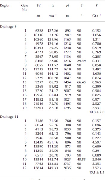
The error sources in our ice-flux estimates include the uncertainties in ice thickness and InSAR velocity. In this area, ice surface velocity is estimated to be in error by ±10ma–1. The low uncertainty is justified based on excellent agreement between the direction of InSAR velocity vectors and the orientation of flow stripes on SAR imagery. It is unlikely that both components of the velocity vector could be substantially in error and in such a way as to retain the expected flow direction. The ice thickness is computed by applying isostasy to the elevation data. Error sources include the uncertainty in the original DEM, column-averaged ice density and the geoid model (Reference Wen, Jezek, Monaghan, Sun, Ren and HuybrechtsWen and others, 2007). Together, these errors yield an overall uncertainty of up to 100m in ice thickness. The resultant error in ice fluxes across the grounding lines is given as 10%.
Notes: W is gate width, U Ū is average surface velocity, H H̄ is mean ice thickness, θ is angle between flow direction and gate, and F is ice flux, converted using a column-averaged ice density of 910 kgm–3.
Total accumulation
We estimate total accumulation by averaging surface accumulation datasets by Reference Thompson and PollardVaughan and others (1999) and M.B. Giovinetto (Reference Giovinetto and ZwallyGiovinetto and Zwally (2000), modified by Giovinetto) (hereafter, Vaughan and Giovinetto compilations respectively). The total accumulations of drainages 9 and 11 (Table 2) are equal to their area multiplied by the annual accumulation rate averaged over the area. The error of the annual accumulation is assumed to be 10%, and the error of the drainage area 5%, so the error in the catchment-wide accumulation totals is 11.2% (Reference WenWen and others, 2006, Reference Wen, Jezek, Monaghan, Sun, Ren and Huybrechts2007).
Table 2. Accumulation, ice fluxes and mass budgets (Gt a–1) for drainages 9, 10 and 11 and the whole grounded ice
Mass Budget of the Grounded Ice
If we assume a steady-state glacier system, the mass output (discharge) (![]() in
out) from an area is equal to the sum of the
in
out) from an area is equal to the sum of the
inflow (![]() in) and the integrated accumulation over the area (Reference Budd and WarnerBudd and Warner, 1996; Reference Fricker, Warner and AllisonFricker and others, 2000b):
in) and the integrated accumulation over the area (Reference Budd and WarnerBudd and Warner, 1996; Reference Fricker, Warner and AllisonFricker and others, 2000b):
where A is annual accumulation rate.
Mass budget of the whole grounded ice
Calculating the mass budget of the grounded ice as a whole, ![]() in
out in Equation (1) is the ice flux across the grounding line,
in
out in Equation (1) is the ice flux across the grounding line, ![]() in
in is 0 and
s A dS is the sum of the total accumulations for drainages 9, 10 and 11.
in
in is 0 and
s A dS is the sum of the total accumulations for drainages 9, 10 and 11.
We evaluate Equation (1) using the results presented in Tables 1 and 2. We find that ![]() = 88.9±8.9 Gt a–1, and
= 88.9±8.9 Gt a–1, and ![]() in
in +
s A dS = 84.8±4.2 Gt a–1 (Table 2). This implies that LAS grounded ice has a statistically insignificant imbalance of –4.2±9.8 Gt a–1, corresponding to –5±12% of the total accumulation.
in
in +
s A dS = 84.8±4.2 Gt a–1 (Table 2). This implies that LAS grounded ice has a statistically insignificant imbalance of –4.2±9.8 Gt a–1, corresponding to –5±12% of the total accumulation.
Mass budgets of three drainages
Table 2 lists the accumulation, ice fluxes and mass budgets for drainages 9, 10 and 11. Drainage 11 has an imbalance of 0.9±2.3 Gt a–1, while drainages 9 and 10 tend towards a negative imbalance, though none of the estimated balance magnitudes are statistically different from zero. Notice that the total area of the grounded ice in drainages 9 and 11 is 371 955 km2, or 27.7% of the entire LAS grounded ice, while the total annual accumulation and ice flux across the grounding lines of these sectors is 40% of the entire grounded LAS. Therefore, drainages 9 and 11 are important components of the system-wide mass balance.
Mass budgets upstream and downstream of the LGB traverse
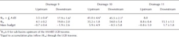
Table 3 gives the mass budgets of the three drainages upstream (as discussed by Wen and others, 2006) and downstream of the Australian LGB traverse. Data used to subdivide the basin include ANARE program ice thicknesses and GPS velocities (Reference Higham and CravenHigham and Craven, 1997; Reference Craven, Higham and BrocklesbyCraven and others, 2001; Reference JezekKiernan, 2001). GPS velocities are supplemented by InSAR velocities. Unlike ice streams draining into the Ross Ice Shelf or the Amundsen Sea, the combined mass budgets of the six upstream and downstream sectors are insignificantly different from zero. That said, there is some variability between the upstream and downstream regions. Sub-basins upstream of drainages 9 and 11 and downstream of drainages 9 and 10 may have a negative imbalance, while regions upstream of drainage 10 and downstream of drainage 11 have a positive imbalance. The upstream region as a whole has an imbalance of 4.4± 6.3 Gt a–1, while the downstream region has a negative imbalance, –8.9±9.9 Gt a–1.
Table 3. Accumulation, ice fluxes and mass budgets (Gt a–1 ) for drainages 9, 10 and 11 upstream and downstream of the ANARE LGB traverse
Conclusions And Discussion
In this paper, we calculate the ice fluxes across the grounding lines of drainages 9 and 11, along with the drainage surface accumulation fluxes. We also calculate the mass budget of the entire grounded ice region of the LAS.
The ice fluxes across the grounding lines of drainages 9 and 11 are 15.1±1.5 Gt a–1 and 19.8±2.0 Gt a–1 respectively. The entire LAS grounded ice is approximately in balance, with a mass budget of –4.2±9.8 Gt a–1. Drainages 9, 10 and 11 are also nearly in balance, with mass budgets of –2.5±2.8 Gt a–1, –2.6±7.8 Gt a–1 and 0.9±2.3 Gt a–1 respectively, though there is some variability between adjacent glaciers upstream and downstream of the ANARE LGB traverse. Although the total grounded-ice area of drainages 9 and 11 covers 27.7% of the entire LAS grounded ice, the total annual accumulation and the total ice flux across the grounding line of these drainages accounts for 40% of the grounded LAS.
Using the integrated approach (ISMASS Committee, 2004), Reference Wu and JezekZwally and others (2005) calculated the net mass balance of the grounded ice in the LAS to be only 0.3 Gt a–1 from 1992 to 2002. Reference WenWen and others (2006) report an overall thickening trend in the basin from 1992 to 2003 of 9.0±1.3 Gt a–1, based on altimetry-derived ice-thickness changes at the grounded LAS based on Reference Davis, Li, McConnell, Frey and HannaDavis and others’ (2005) supporting online material. In this paper, we estimate the mass budget of the grounded ice to be –4.2±9.8 Gt a–1 using a component approach (ISMASS Committee, 2004). Some of the differences may arise because of different estimates of the net surface balance. Reference Wu and JezekZwally and others (2005) estimated the total accumulation of the grounded ice in the LAS to be 79.61 Gt a–1, 5 Gt a–1 less than our result. Possible explanations include: (1) they used surface annual accumulation data compiled by Reference Giovinetto and ZwallyGiovinetto and Zwally (2000), while we used the average of Vaughan and Giovinetto compilations; and (2) there are some differences in the grounding line position and the coverage of the LAS between the two studies. The remaining differences are more difficult to explain. However, we believe our sector-by-sector analysis of LAS mass balance gives a more complete picture of basin properties and offers a contrast to West Antarctica where there seem to be strong flow-regime-to-flow-regime mass-balance differences.
Acknowledgements
This work is supported by the National Natural Science Foundation of China (grants No. 40730526, 40471028, 40476005), the Shu Guang project (grant No. 05SG46) and NASA’s Polar Oceans and Ice Sheets Program. We thank M.B. Giovinetto and D.G. Vaughan for providing accumulation compilations. In particular, M.B. Giovinetto provided a new modified (as yet unpublished) accumulation compilation.


