


1. Introduction
Controlling wall-bounded turbulent flows is an active area of research (Adrian Reference Adrian2007; Hutchins & Marusic Reference Hutchins and Marusic2007a ; Marusic et al. Reference Marusic, McKeon, Monkewitz, Nagib, Smits and Sreenivasan2010; Barkley et al. Reference Barkley, Song, Mukund, Lemoult, Avila and Hof2015), due to its practical importance. For example, in the turbulent boundary layer (TBL) class of wall-bounded turbulent flows investigated in this study, TBL control devices are used to improve transport speed and fuel efficiency via reducing viscous drag in engineering applications, such as flows over aircraft wings and ship hulls (Chung et al. Reference Chung, Hutchins, Schultz and Flack2021). Control strategies include passive techniques that introduce perturbation without additional energy input (Corke & Thomas Reference Corke and Thomas2018), such as riblets and large-eddy breakup devices (LEBUs). Existing passive control devices increase device drag (a type of form drag), such that it is challenging to achieve a reduction in total drag, i.e. viscous plus device drag from control devices (García-Mayoral & Jiménez Reference García-Mayoral and Jiménez2011; Park et al. Reference Park, An, Hutchins, Choi, Chun and Lee2011; Saravi & Cheng Reference Saravi and Cheng2013; Chin et al. Reference Chin, Örlü, Monty, Hutchins, Ooi and Schlatter2017). Active flow control is an alternative approach, which requires additional energy input, such as plasma/blowing–suction walls (Antonia et al. Reference Antonia, Krishnamoorthy, Fulachier, Benabid and Anselmet1988; Djenidi, Kamruzzaman & Dostal Reference Djenidi, Kamruzzaman and Dostal2019). Active control strategies incur negligible device drag and reduce total drag. Under certain conditions, the power saving from the total drag reduction covers the energy input, leading to positive net power savings. For instance, plasma actuation has demonstrated substantial net power savings, achieving friction drag reductions of up to 70 % (Thomas, Corke & Duong Reference Thomas, Corke and Duong2023), while wall oscillation techniques have similarly provided net energy benefits, with drag reductions of up to 25 % (Chandran et al. Reference Chandran, Zampiron, Rouhi, Fu, Wine, Holloway, Smits and Marusic2023). Despite these examples, the energy requirements of most active methods remain a barrier to practical application (Corke & Thomas Reference Corke and Thomas2018). In addition, they often need complicated control systems to work well under different flow conditions (Corke & Thomas Reference Corke and Thomas2018).
Motivated by the challenges involved in active and passive flow control techniques, theoretical, numerical and experimental studies have been performed over the past decade to gain a better understanding of the contributions of the small- and large-eddy motions towards viscous drag (Hutchins & Marusic Reference Hutchins and Marusic2007a
; Marusic et al. Reference Marusic, McKeon, Monkewitz, Nagib, Smits and Sreenivasan2010; Mathis et al. Reference Mathis, Marusic, Chernyshenko and Hutchins2013; Chandran, Monty & Marusic Reference Chandran, Monty and Marusic2020; Chung et al. Reference Chung, Hutchins, Schultz and Flack2021). Near-wall structures, comprising quasistreamwise vortices and low-speed streaks within the viscous sublayer, buffer and lower logarithmic layers, are generated through a self-sustaining cycle, in which vortices create streaks by lifting and redistributing momentum. The streaks undergo instability and disturbance amplification, and the resulting motions generate new vortices that restart the cycle (Robinson Reference Robinson1991; Jiménez & Pinelli Reference Jiménez and Pinelli1999; Schoppa & Hussain Reference Schoppa and Hussain2002). Large-scale motions consist of streamwise-aligned hairpin eddies with a length scale of the order of $\delta$
, while superstructures in TBLs extend up to
$\delta$
, while superstructures in TBLs extend up to $20\delta$
(Adrian Reference Adrian2007; Hutchins & Marusic Reference Hutchins and Marusic2007a
). The large-scale structures, including hairpin-shaped structures and superstructures, have modulation effects on the small-scale structures in the near-wall region, which account for the majority of the total viscous drag (Hutchins & Marusic Reference Hutchins and Marusic2007b
; Mathis, Hutchins & Marusic Reference Mathis, Hutchins and Marusic2009; Agostini & Leschziner Reference Agostini and Leschziner2018). Hence, attenuating either near-wall small-scale structures or large-scale structures in the outer region could lead to viscous drag reduction (Agostini & Leschziner Reference Agostini and Leschziner2018). This has underpinned the design of flow control devices to reduce viscous drag, particularly in the field of passive control strategies, which includes LEBUs that attenuate large-scale motions in the outer region far downstream, although they still induce considerable device drag (Perlin, Dowling & Ceccio Reference Perlin, Dowling and Ceccio2016).
$20\delta$
(Adrian Reference Adrian2007; Hutchins & Marusic Reference Hutchins and Marusic2007a
). The large-scale structures, including hairpin-shaped structures and superstructures, have modulation effects on the small-scale structures in the near-wall region, which account for the majority of the total viscous drag (Hutchins & Marusic Reference Hutchins and Marusic2007b
; Mathis, Hutchins & Marusic Reference Mathis, Hutchins and Marusic2009; Agostini & Leschziner Reference Agostini and Leschziner2018). Hence, attenuating either near-wall small-scale structures or large-scale structures in the outer region could lead to viscous drag reduction (Agostini & Leschziner Reference Agostini and Leschziner2018). This has underpinned the design of flow control devices to reduce viscous drag, particularly in the field of passive control strategies, which includes LEBUs that attenuate large-scale motions in the outer region far downstream, although they still induce considerable device drag (Perlin, Dowling & Ceccio Reference Perlin, Dowling and Ceccio2016).
Miniature vortex generators (MVGs) are a promising approach for passive flow control without significantly increasing device drag (Lin Reference Lin2002). The MVG technique comprises a spanwise-aligned MVG array consisting of two blades vertically mounted on a wall and positioned at a certain ‘attack angle’ to the flow. The ‘miniature’ of MVG refers to the low ratio of MVG height $h$
to boundary layer thickness
$h$
to boundary layer thickness $\delta$
. The MVGs are typically defined as
$\delta$
. The MVGs are typically defined as $h/\delta _0\leqslant 0.2$
(Lin Reference Lin1999), where
$h/\delta _0\leqslant 0.2$
(Lin Reference Lin1999), where $\delta _0$
is the boundary layer thickness at the MVG location. In contrast, devices with ratios
$\delta _0$
is the boundary layer thickness at the MVG location. In contrast, devices with ratios $h/\delta _0\geqslant 0.5$
are classified as vortex generators (VGs), and those with ratios
$h/\delta _0\geqslant 0.5$
are classified as vortex generators (VGs), and those with ratios $0.2\lt h/\delta _0\lt 0.5$
are referred to as low-profile VGs (Chan & Chin Reference Chan and Chin2022). The MVG height ratio is one of the most important parameters correlating with the strength and size of the MVG-induced vortex (Lin Reference Lin2002; Godard & Stanislas Reference Godard and Stanislas2006).
$0.2\lt h/\delta _0\lt 0.5$
are referred to as low-profile VGs (Chan & Chin Reference Chan and Chin2022). The MVG height ratio is one of the most important parameters correlating with the strength and size of the MVG-induced vortex (Lin Reference Lin2002; Godard & Stanislas Reference Godard and Stanislas2006).
The MVGs were first introduced to reduce form drag caused by flow separation in laminar and TBL flows, when a fluid moves over a bluff body, such as when air flows over aerofoils (Lin et al. Reference Lin, Robinson, McGhee and Valarezo1994). Optimised MVG configurations can substantially reduce form drag in aerofoil applications, such that total drag (including viscous and device drag) is halved (Godard & Stanislas Reference Godard and Stanislas2006). When MVGs are applied to road vehicles, where the total drag is dominated by viscous drag, the total drag reduction can still reach up to 10 % (Sudin et al. Reference Sudin, Abdullah, Shamsuddin, Ramli and Tahir2014). The MVGs have also been used to reduce viscous drag in transitional boundary layers by delaying the flow from transition to turbulence (Fransson & Talamelli Reference Fransson and Talamelli2012; Shahinfar et al. Reference Shahinfar, Fransson, Sattarzadeh and Talamelli2013). The proposed mechanism is that MVGs impose large-scale vortical motions and incur long high- and low-speed streaks, which can stabilise the Tollmien–Schlichting wave formation and delay the turbulence formation by prolonging the transition progress (Shahinfar et al. Reference Shahinfar, Fransson, Sattarzadeh and Talamelli2013). The MVG-induced streaks propagate downstream as far as 700 times the MVG height, and the high-speed streaks can reduce turbulence intensity by stabilising the developing turbulence in the near-wall region (Fransson & Talamelli Reference Fransson and Talamelli2012). A configuration with two consecutive MVG arrays delays transition by over 3000 times the MVG height, achieving up to 65 % total drag reduction over a 4 m reference length, compared with the smooth-wall case without MVGs (Sattarzadeh et al. Reference Sattarzadeh, Fransson, Talamelli and Fallenius2014).
The turbulence structures and velocity fluctuation amplitudes in TBLs differ from those in transitional boundary layers (Schlichting & Gersten Reference Schlichting and Gersten2016; Lee & Jiang Reference Lee and Jiang2019), indicating that the effects of MVG-induced vortices may differ from that in transitional boundary layers. Therefore, it is necessary to explore the MVG effects in TBL flows, particularly in turbulence structure manipulations. In a related study, Lögdberg et al. (Reference Lögdberg, Fransson and Alfredsson2009) conducted an experiment on VGs in TBLs ( $h/\delta _0\gt 0.2$
), focusing on vortex evolution for flow separation. They found that a VG-induced streamwise vortex developed in the near-wall region at a friction Reynolds number
$h/\delta _0\gt 0.2$
), focusing on vortex evolution for flow separation. They found that a VG-induced streamwise vortex developed in the near-wall region at a friction Reynolds number ${\textit{Re}}_\tau \approx 3000$
. Since their study, understanding of turbulence structures has advanced considerably (Jiménez Reference Jiménez2018; Marusic & Monty Reference Marusic and Monty2019). Based on these advances, Chan & Chin (Reference Chan and Chin2022) explored MVG control effects on turbulence motions in TBL flows using a large-eddy simulation (LES) approach. Their results suggest that the MVG-induced motions interrupt the near-wall cycle structures dominating the near-wall region of a flat plat TBL. Although the spanwise-averaged drag is nearly the same as that of a smooth wall, there is a LES study that reported a local drag reduction in the spanwise direction, particularly in the upwash region (Chan & Chin Reference Chan and Chin2022).
${\textit{Re}}_\tau \approx 3000$
. Since their study, understanding of turbulence structures has advanced considerably (Jiménez Reference Jiménez2018; Marusic & Monty Reference Marusic and Monty2019). Based on these advances, Chan & Chin (Reference Chan and Chin2022) explored MVG control effects on turbulence motions in TBL flows using a large-eddy simulation (LES) approach. Their results suggest that the MVG-induced motions interrupt the near-wall cycle structures dominating the near-wall region of a flat plat TBL. Although the spanwise-averaged drag is nearly the same as that of a smooth wall, there is a LES study that reported a local drag reduction in the spanwise direction, particularly in the upwash region (Chan & Chin Reference Chan and Chin2022).
From the view of induced flow structures, generating large-scale streamwise vortices (LSSVs) using control devices has emerged as an effective strategy for viscous drag reduction in TBL flows. This concept was originally proposed by Schoppa & Hussain (Reference Schoppa and Hussain1998) in the context of direct numerical simulations for turbulent channel flows. They introduced LSSVs through two approaches: (i) counter-rotating vortex forcing in the outer region; and (ii) spanwise wall-jet forcing on the wall. Both methods induce strong spanwise motions and achieved drag reductions of up to 20 % and 50 %, respectively. This strategy is employed in active flow control methods using plasma actuators, which generate near-wall jets that effectively suppress quasistreamwise vortices in TBLs. For instance, Cheng et al. (Reference Cheng, Wong, Hussain, Schröder and Zhou2021) demonstrated global drag reductions up to 26 % by inducing spanwise arrays of LSSVs, while Duong, Corke & Thomas (Reference Duong, Corke and Thomas2021) achieved over 60 % global drag reduction using pulsed-direct-current plasma actuators. Cheng et al. (Reference Cheng, Wong, Hussain, Schröder and Zhou2021) suggested that the global drag reduction is associated with the lifting of low-speed fluid in the upwash region and the LSSV-induced spanwise motions between upwash and downwash regions. The lifted low-speed fluid reduces near-wall streamwise velocity gradients, thereby reducing drag, while the induced spanwise motions weaken wall-normal vorticity and disrupt the streak transient growth mechanism, consistent with the viscous drag reduction strategy proposed by Schoppa & Hussain (Reference Schoppa and Hussain1998). Both studies found decreases in streamwise and spanwise turbulence intensities, as well as reductions in turbulence production near the wall, confirming the effectiveness of LSSVs for viscous drag reduction. This strategy highlights the potential of MVG-induced streamwise vortical structures for drag reduction in TBLs.
The modulation of near-wall flow disturbance by MVGs and the local drag reduction observed in the upwash motions associated with the MVG-induced LSSVs indicates that the MVGs can be explored for TBL flow control (Cheng et al. Reference Cheng, Wong, Hussain, Schröder and Zhou2021; Chan & Chin Reference Chan and Chin2022). However, due to the high computational cost of LES, only one LES experiment was performed by Chan & Chin (Reference Chan and Chin2022) and the friction Reynolds number was limited to ${\textit{Re}}_\tau =950$
. Therefore, the effects of important parameters on the outer-region turbulence structures remain unclear, particularly the influence of the MVG height ratio and the effects at higher friction Reynolds numbers,
${\textit{Re}}_\tau =950$
. Therefore, the effects of important parameters on the outer-region turbulence structures remain unclear, particularly the influence of the MVG height ratio and the effects at higher friction Reynolds numbers, ${\textit{Re}}_\tau \gt 950$
. According to the wall shear stress model proposed by Marusic et al. (Reference Marusic, Chandran, Rouhi, Fu, Wine, Holloway, Chung and Smits2021), small-scale structures dominate the contribution to the total shear stress, whereas large-scale structures account for up to 30 %. Therefore, it is important to characterise how MVGs modulate turbulence structures.
${\textit{Re}}_\tau \gt 950$
. According to the wall shear stress model proposed by Marusic et al. (Reference Marusic, Chandran, Rouhi, Fu, Wine, Holloway, Chung and Smits2021), small-scale structures dominate the contribution to the total shear stress, whereas large-scale structures account for up to 30 %. Therefore, it is important to characterise how MVGs modulate turbulence structures.
In this study, we perform a series of experiments on MVGs in TBLs to gain understanding of how the MVG height ratio and the Reynolds number affect turbulence structures. We test two height ratios, $h/\delta _0=0.09$
and
$h/\delta _0=0.09$
and $0.18$
, and a range of Reynolds numbers from
$0.18$
, and a range of Reynolds numbers from ${\textit{Re}}_\tau =400$
–
${\textit{Re}}_\tau =400$
– $2000$
for zero pressure gradient (ZPG) MVG-modified TBLs, and measure the downstream flow fields at various stations. We use a recently proposed friction velocity determination method (Kong et al. Reference Kong, Nugroho, Bennetts, Chan and Chin2024) to derive the inner-scaling turbulence structures, which are not directly available from experimental measurements. We find the MVGs attenuate an increasing proportion of turbulence energy as Reynolds number increases, which implies the MVGs have the potential to control turbulence structures in TBLs.
$2000$
for zero pressure gradient (ZPG) MVG-modified TBLs, and measure the downstream flow fields at various stations. We use a recently proposed friction velocity determination method (Kong et al. Reference Kong, Nugroho, Bennetts, Chan and Chin2024) to derive the inner-scaling turbulence structures, which are not directly available from experimental measurements. We find the MVGs attenuate an increasing proportion of turbulence energy as Reynolds number increases, which implies the MVGs have the potential to control turbulence structures in TBLs.
2. Experimental set-up
2.1. Wind tunnel
The ZPG MVG-modified TBL experiments are performed in the closed-loop wind tunnel at the University of Adelaide. The airflow goes through three layers of meshes and one layer of honeycomb grid, which can maintain a low turbulence level of approximately $0.5\,\%$
. A working section is attached to the wind tunnel, having a length of
$0.5\,\%$
. A working section is attached to the wind tunnel, having a length of $2$
m and a rectangular cross-sectional area of
$2$
m and a rectangular cross-sectional area of $0.5 \times 0.3\,$
m
$0.5 \times 0.3\,$
m $^{2}$
. A
$^{2}$
. A $1.9$
m-long aluminium flat plate is mounted on the bottom floor of the working section. The sidewalls are adjustable to compensate for the boundary layer growth to maintain ZPG. A tripping device of 36-grit sandpaper of length
$1.9$
m-long aluminium flat plate is mounted on the bottom floor of the working section. The sidewalls are adjustable to compensate for the boundary layer growth to maintain ZPG. A tripping device of 36-grit sandpaper of length $100$
mm is mounted at the leading edge to ensure flows develop to TBLs.
$100$
mm is mounted at the leading edge to ensure flows develop to TBLs.
Schematic views of the MVG configuration and experimental set-up for MVG (a,b) and reference TBLs (c). The value of $x_0$
for the two MVG height ratios is defined from the trailing edge of the tripping device to the trailing edge of MVG blades. Measurement
$x_0$
for the two MVG height ratios is defined from the trailing edge of the tripping device to the trailing edge of MVG blades. Measurement $yz$
–planes downstream the MVG devices are denoted as the planes at
$yz$
–planes downstream the MVG devices are denoted as the planes at $x^*=x-x_0=5\,\text{h}$
, 25, 50, 100, 200 and
$x^*=x-x_0=5\,\text{h}$
, 25, 50, 100, 200 and $500\,\text{h}$
. At each streamwise station, six linear-spaced spanwise velocity profiles are measured at
$500\,\text{h}$
. At each streamwise station, six linear-spaced spanwise velocity profiles are measured at $z=0$
–
$z=0$
– $0.5\varLambda _z$
. The reference TBL results are measured over a flat plate at corresponding streamwise stations of the MVG result, in which the black and red annotations denote the streamwise stations scaled by the two MVG placements
$0.5\varLambda _z$
. The reference TBL results are measured over a flat plate at corresponding streamwise stations of the MVG result, in which the black and red annotations denote the streamwise stations scaled by the two MVG placements $x_0=0.41$
m and
$x_0=0.41$
m and $1.31$
m, respectively.
$1.31$
m, respectively.

2.2. The MVG configurations
The schematic of the MVG and reference TBL measurement settings is shown in figure 1. The Cartesian coordinates $x$
,
$x$
, $y$
and
$y$
and $z$
correspond to the streamwise, wall-normal and spanwise directions, respectively. The coordinate system is chosen with the origin at the leading edge centreline of the aluminium flat plate. The effectiveness of vane-type MVGs in maximising circulation amplitude for flow-separation control has been extensively studied, focusing on optimising geometric parameters such as blade aspect ratio,
$z$
correspond to the streamwise, wall-normal and spanwise directions, respectively. The coordinate system is chosen with the origin at the leading edge centreline of the aluminium flat plate. The effectiveness of vane-type MVGs in maximising circulation amplitude for flow-separation control has been extensively studied, focusing on optimising geometric parameters such as blade aspect ratio, $L/h$
, angle of attack (AOA), spanwise distance between MVG pairs,
$L/h$
, angle of attack (AOA), spanwise distance between MVG pairs, $D$
, and spanwise wavelength of MVG pairs,
$D$
, and spanwise wavelength of MVG pairs, $\varLambda _z$
(Pearcey Reference Pearcey1961; Godard & Stanislas Reference Godard and Stanislas2006). The AOA intensifies the circulation of MVG-induced vortices, enhancing flow control as it increases; however, AOAs exceeding
$\varLambda _z$
(Pearcey Reference Pearcey1961; Godard & Stanislas Reference Godard and Stanislas2006). The AOA intensifies the circulation of MVG-induced vortices, enhancing flow control as it increases; however, AOAs exceeding $18^\circ$
can cause excessive instability in transition control applications. Consequently, an optimal AOA range of
$18^\circ$
can cause excessive instability in transition control applications. Consequently, an optimal AOA range of $15^\circ$
–
$15^\circ$
– $18^\circ$
is recommended, aligning with studies on flow separation and transition control (Pauley & Eaton Reference Pauley and Eaton1988; Godard & Stanislas Reference Godard and Stanislas2006; Sattarzadeh & Fransson Reference Sattarzadeh and Fransson2015). The blade aspect ratio,
$18^\circ$
is recommended, aligning with studies on flow separation and transition control (Pauley & Eaton Reference Pauley and Eaton1988; Godard & Stanislas Reference Godard and Stanislas2006; Sattarzadeh & Fransson Reference Sattarzadeh and Fransson2015). The blade aspect ratio, $L/h$
, has a minimal effect on vortex circulation amplitude, with a suggested value of 2.5 (Pearcey Reference Pearcey1961). For spanwise wavelength, configurations with
$L/h$
, has a minimal effect on vortex circulation amplitude, with a suggested value of 2.5 (Pearcey Reference Pearcey1961). For spanwise wavelength, configurations with $\varLambda _z/h = 10$
and
$\varLambda _z/h = 10$
and $\varLambda _z/D = 4$
are recommended to achieve a long effective distance range while effectively suppressing flow separation (Pearcey Reference Pearcey1961). Furthermore, Fransson & Talamelli (Reference Fransson and Talamelli2012) and Shahinfar et al. (Reference Shahinfar, Fransson, Sattarzadeh and Talamelli2013) advocate for spanwise wavelength ratios of
$\varLambda _z/D = 4$
are recommended to achieve a long effective distance range while effectively suppressing flow separation (Pearcey Reference Pearcey1961). Furthermore, Fransson & Talamelli (Reference Fransson and Talamelli2012) and Shahinfar et al. (Reference Shahinfar, Fransson, Sattarzadeh and Talamelli2013) advocate for spanwise wavelength ratios of $\varLambda _z/D = 4$
–5 for MVG pairs to establish an effective vortex pattern across the entire spanwise length. Lower
$\varLambda _z/D = 4$
–5 for MVG pairs to establish an effective vortex pattern across the entire spanwise length. Lower $\varLambda _z/D$
ratios can lead to vortex collisions and ejection from the wall, whereas higher
$\varLambda _z/D$
ratios can lead to vortex collisions and ejection from the wall, whereas higher $\varLambda _z/D$
ratios result in MVG-induced vortices developing individually without covering the full wavelength, thereby diminishing their effectiveness.
$\varLambda _z/D$
ratios result in MVG-induced vortices developing individually without covering the full wavelength, thereby diminishing their effectiveness.
In the present study, the metal MVG blades are spanwise arranged as a total of 13 pairs of MVGs and affixed on the flat aluminium plate at streamwise locations, $x_0$
. Consistent with the LES study by Chan & Chin (Reference Chan and Chin2022), the rectangular vane-type MVG blades have dimensions of height
$x_0$
. Consistent with the LES study by Chan & Chin (Reference Chan and Chin2022), the rectangular vane-type MVG blades have dimensions of height $h=3$
mm, thickness of
$h=3$
mm, thickness of $w=0.75$
mm and length of
$w=0.75$
mm and length of $L=7.5$
mm, resulting in a blade aspect ratio
$L=7.5$
mm, resulting in a blade aspect ratio $L/h=2.5$
, as recommended by Pearcey (Reference Pearcey1961). The blades are arranged with an AOA of
$L/h=2.5$
, as recommended by Pearcey (Reference Pearcey1961). The blades are arranged with an AOA of $15^\circ$
. The spanwise distance between the centroids of MVG blades within a single pair is
$15^\circ$
. The spanwise distance between the centroids of MVG blades within a single pair is $D=7.5$
mm, and the spanwise wavelength between MVG pairs
$D=7.5$
mm, and the spanwise wavelength between MVG pairs $\varLambda _z=30$
mm. These configurations adhere to the recommended ratios of
$\varLambda _z=30$
mm. These configurations adhere to the recommended ratios of $\varLambda _z/D=4$
and
$\varLambda _z/D=4$
and $\varLambda _z/h=10$
as suggested by Pearcey (Reference Pearcey1961) and Sattarzadeh & Fransson (Reference Sattarzadeh and Fransson2015), ensuring effective vortex formation and flow control performance.
$\varLambda _z/h=10$
as suggested by Pearcey (Reference Pearcey1961) and Sattarzadeh & Fransson (Reference Sattarzadeh and Fransson2015), ensuring effective vortex formation and flow control performance.
The MVG experiments are performed by placing the MVG array at two streamwise locations, $x_0=0.41$
m and
$x_0=0.41$
m and $1.31$
m. Two MVG-TBL measurements are operated at two free stream velocities
$1.31$
m. Two MVG-TBL measurements are operated at two free stream velocities $U_\infty =7.4$
and
$U_\infty =7.4$
and $20$
m s
$20$
m s $^{-1}$
at two MVG locations. Note that an additional MVG experiment is performed for the Reynolds number matching purpose by operating a moderate free stream velocity
$^{-1}$
at two MVG locations. Note that an additional MVG experiment is performed for the Reynolds number matching purpose by operating a moderate free stream velocity $U_\infty =11$
m s
$U_\infty =11$
m s $^{-1}$
with the MVGs arranged at
$^{-1}$
with the MVGs arranged at $x_0=1.31$
m. The boundary layer thickness
$x_0=1.31$
m. The boundary layer thickness $\delta$
is the distance from the wall to the position based on
$\delta$
is the distance from the wall to the position based on $99\,\%$
of the free stream velocity. For the front and back MVG locations, the MVG height ratios are
$99\,\%$
of the free stream velocity. For the front and back MVG locations, the MVG height ratios are $h/\delta _0\approx 0.18$
and
$h/\delta _0\approx 0.18$
and $0.09$
, respectively, where the higher
$0.09$
, respectively, where the higher $h/\delta _0\approx 0.18$
is similar to those used by Chan & Chin (Reference Chan and Chin2022). The friction Reynolds numbers at the MVG locations vary from
$h/\delta _0\approx 0.18$
is similar to those used by Chan & Chin (Reference Chan and Chin2022). The friction Reynolds numbers at the MVG locations vary from $400$
to
$400$
to $1600$
in the five sets of experiments to investigate the Reynolds number effects at the MVG placement. A summary of the flow condition detail and the MVG dimensions are found in table 1. Note that the superscript and subscript of the case name are referred to as the values of the MVG height ratio and the friction Reynolds number. For example, the case of
$1600$
in the five sets of experiments to investigate the Reynolds number effects at the MVG placement. A summary of the flow condition detail and the MVG dimensions are found in table 1. Note that the superscript and subscript of the case name are referred to as the values of the MVG height ratio and the friction Reynolds number. For example, the case of $\text{MVG}_{400}^{18}$
represents conditions at
$\text{MVG}_{400}^{18}$
represents conditions at ${\textit{Re}}_\tau =400$
and
${\textit{Re}}_\tau =400$
and $h/\delta _0\approx 0.18$
, similar to those of the LES study (Chan & Chin Reference Chan and Chin2022).
$h/\delta _0\approx 0.18$
, similar to those of the LES study (Chan & Chin Reference Chan and Chin2022).
Experimental conditions and MVG configurations. Here $\delta _0$
is the boundary layer thickness at
$\delta _0$
is the boundary layer thickness at $x=x_0$
.
$x=x_0$
.

2.3. Measurement grid set-up
The wall-normal and spanwise flow fields ( $yz$
-plane) are measured at several streamwise stations downstream of the MVG array, as shown in figure 1(a,b). For each
$yz$
-plane) are measured at several streamwise stations downstream of the MVG array, as shown in figure 1(a,b). For each $yz$
-plane, we conduct six linear-spaced spanwise velocity profile measurements at
$yz$
-plane, we conduct six linear-spaced spanwise velocity profile measurements at $z/\varLambda _z=0$
–
$z/\varLambda _z=0$
– $0.5$
, enough to characterise the spanwise-varied TBLs downstream of the MVGs and obtain the spanwise- and temporal-averaged profiles (also referred to as ‘global profiles’) with a low uncertainty level of
$0.5$
, enough to characterise the spanwise-varied TBLs downstream of the MVGs and obtain the spanwise- and temporal-averaged profiles (also referred to as ‘global profiles’) with a low uncertainty level of $\lt 3.5\,\%$
at each
$\lt 3.5\,\%$
at each $yz$
-plane (Kong et al. Reference Kong, Nugroho, Bennetts, Chan and Chin2024). The study by Kong et al. (Reference Kong, Nugroho, Bennetts, Chan and Chin2024) provides evidence that six spanwise locations are sufficient for the MVG configuration used in our work. Six
$yz$
-plane (Kong et al. Reference Kong, Nugroho, Bennetts, Chan and Chin2024). The study by Kong et al. (Reference Kong, Nugroho, Bennetts, Chan and Chin2024) provides evidence that six spanwise locations are sufficient for the MVG configuration used in our work. Six $yz$
-planes are measured at
$yz$
-planes are measured at $x^*/h=5$
, 25, 50, 100, 200 and 500, where
$x^*/h=5$
, 25, 50, 100, 200 and 500, where $x^*$
is the streamwise distance from the trailing edge of the MVG array,
$x^*$
is the streamwise distance from the trailing edge of the MVG array, $x^*=x-x_0$
. For the cases with
$x^*=x-x_0$
. For the cases with $h/\delta _0=0.09$
, the MVGs are placed farther downstream at
$h/\delta _0=0.09$
, the MVGs are placed farther downstream at $x_0=1.31$
m and the streamwise measurement station is limited to
$x_0=1.31$
m and the streamwise measurement station is limited to $x^*/h\leqslant 200$
due to the length limitation of the test section. The wall-normal velocity profiles are taken from the near-wall position
$x^*/h\leqslant 200$
due to the length limitation of the test section. The wall-normal velocity profiles are taken from the near-wall position $y\approx 0.2$
mm to
$y\approx 0.2$
mm to $y\approx 1.5\delta$
with varying measurement points of 30–50. Hence, the total number of grid points varies from 180–300 (
$y\approx 1.5\delta$
with varying measurement points of 30–50. Hence, the total number of grid points varies from 180–300 ( $6\times 30$
–
$6\times 30$
– $6\times 50$
) for different streamwise stations.
$6\times 50$
) for different streamwise stations.
2.4. Traverse system
The two-dimensional traverse system comprises horizontal and vertical sliding platforms equipped with two optical linear encoders and driven by microstepper motors, which can perform horizontal and vertical traverses of the sensor probe accurate to $5$
and
$5$
and $0.5$
μm, respectively. For each wall-normal velocity profile measurement, the wall distance of the sensor probe is determined using a digital microscope. The study of Kong et al. (Reference Kong, Nugroho, Bennetts, Chan and Chin2024) gives the details of the method determining wall distance. The accuracy of the wall distance is
$0.5$
μm, respectively. For each wall-normal velocity profile measurement, the wall distance of the sensor probe is determined using a digital microscope. The study of Kong et al. (Reference Kong, Nugroho, Bennetts, Chan and Chin2024) gives the details of the method determining wall distance. The accuracy of the wall distance is $\leqslant 8$
μm, and the influence of the wall distance error on the
$\leqslant 8$
μm, and the influence of the wall distance error on the $U_\tau$
estimation is reported to be negligible (Kong et al. Reference Kong, Nugroho, Bennetts, Chan and Chin2024).
$U_\tau$
estimation is reported to be negligible (Kong et al. Reference Kong, Nugroho, Bennetts, Chan and Chin2024).
2.5. Velocity measurement
The velocity information is measured using hot-wire anemometry (HWA). Our in-house constant temperature anemometer is based on the design by Perry (Reference Perry1982), and identical to the Melbourne University Constant Temperature Anemometer that has been used by Marusic et al. (Reference Marusic, Monty, Hultmark and Smits2013), Squire et al. (Reference Squire, Morrill-Winter, Hutchins, Schultz, Klewicki and Marusic2016) and Kevin et al. (Reference Kevin, Monty, Bai, Pathikonda, Nugroho, Barros, Christensen and Hutchins2017). The HWA uses a single-wire boundary-type probe with sensor filaments of platinum–wollaston wires and a filament length of $l=0.5$
mm. The HWA system signal is sampled using a National Instrument data acquisition board (NI9234) with frequency
$l=0.5$
mm. The HWA system signal is sampled using a National Instrument data acquisition board (NI9234) with frequency $f_s=51\,200$
Hz and a minimum duration
$f_s=51\,200$
Hz and a minimum duration $T=120$
s. The viscous sampling time and sampling duration satisfy
$T=120$
s. The viscous sampling time and sampling duration satisfy $t^+ =1/f_s(U_\tau ^2/\nu )\lt 1$
and
$t^+ =1/f_s(U_\tau ^2/\nu )\lt 1$
and $TU_\infty \gt 20\,000\delta$
to temporally resolve all high-energy velocity fluctuation and encompass several hundreds of the large-scale events (Hutchins & Marusic Reference Hutchins and Marusic2007a
; Hutchins et al. Reference Hutchins, Nickels, Marusic and Chong2009). The spatial resolution correlates with the inner-scaled sensor length,
$TU_\infty \gt 20\,000\delta$
to temporally resolve all high-energy velocity fluctuation and encompass several hundreds of the large-scale events (Hutchins & Marusic Reference Hutchins and Marusic2007a
; Hutchins et al. Reference Hutchins, Nickels, Marusic and Chong2009). The spatial resolution correlates with the inner-scaled sensor length, $l^+=l U_\tau /\nu$
, which varies from
$l^+=l U_\tau /\nu$
, which varies from $10$
to
$10$
to $25$
for the five data sets. The inner-scaled sensor length of
$25$
for the five data sets. The inner-scaled sensor length of $l^+\leqslant 25$
indicates that the measurements do not experience significant spatial attenuation (e.g. the error of the inner peak amplitude of turbulence intensity is
$l^+\leqslant 25$
indicates that the measurements do not experience significant spatial attenuation (e.g. the error of the inner peak amplitude of turbulence intensity is $\lesssim{10}\,\%$
(Hutchins et al. Reference Hutchins, Nickels, Marusic and Chong2009)). For the mean statistics analysis,
$\lesssim{10}\,\%$
(Hutchins et al. Reference Hutchins, Nickels, Marusic and Chong2009)). For the mean statistics analysis, $U$
and
$U$
and $u^\prime$
denote the time-averaged velocity signal and the velocity fluctuation in the streamwise direction, respectively. Here
$u^\prime$
denote the time-averaged velocity signal and the velocity fluctuation in the streamwise direction, respectively. Here $\langle U\rangle$
and
$\langle U\rangle$
and $\langle u^\prime \rangle$
denote the corresponding spanwise-averaged quantities over half of the spanwise distance of MVG pairs,
$\langle u^\prime \rangle$
denote the corresponding spanwise-averaged quantities over half of the spanwise distance of MVG pairs, $z=0$
–
$z=0$
– $\varLambda _z/2$
. The superscript
$\varLambda _z/2$
. The superscript $+$
indicates the scaling of inner units, for example,
$+$
indicates the scaling of inner units, for example, $U^+=U/U_\tau$
and
$U^+=U/U_\tau$
and $y^+=y/l_v$
, where
$y^+=y/l_v$
, where $l_v=\nu /U_\tau$
is the viscous length scaling.
$l_v=\nu /U_\tau$
is the viscous length scaling.
The velocity measurement processes are automatic and take approximately 10–20 hr for different $yz$
-planes. The calibration is performed every 5 hr of measurement by placing a Pitot tube
$yz$
-planes. The calibration is performed every 5 hr of measurement by placing a Pitot tube $10$
mm above the hot-wire probe into the free stream flow. The free stream velocity is measured using a Pitot tube with an electronic barometer (220DD Baratron, MKS). The flow temperature is monitored by a calibrated RTD-type thermocouple (Pt1000). The calibration profile is determined by fitting a fourth-order polynomial curve onto the pressure and HWA signals. The intermediate calibration profile is then computed by interpolating the precalibration and postcalibration profiles obtained before and after each 5 hr measurement to correct the temperature drift if required (Talluru et al. Reference Talluru, Kulandaivelu, Hutchins and Marusic2014).
$10$
mm above the hot-wire probe into the free stream flow. The free stream velocity is measured using a Pitot tube with an electronic barometer (220DD Baratron, MKS). The flow temperature is monitored by a calibrated RTD-type thermocouple (Pt1000). The calibration profile is determined by fitting a fourth-order polynomial curve onto the pressure and HWA signals. The intermediate calibration profile is then computed by interpolating the precalibration and postcalibration profiles obtained before and after each 5 hr measurement to correct the temperature drift if required (Talluru et al. Reference Talluru, Kulandaivelu, Hutchins and Marusic2014).
2.6. The ZPG smooth-wall flow
The ZPG smooth-wall TBL developed over the aluminium flat plate without the MVGs is used as the reference flow to characterise the MVG effects. The wall-normal velocity profile measurements are performed at the consistent local streamwise stations and free stream velocities to the MVG measurement and referred to as ‘local TBL’, as shown in figure 1. The boundary layer parameters of the local TBL are summarised in table 2.
Boundary layer condition detail of the ZPG smooth-wall TBL (referred to local TBL). The reference local station $x^*/h=(x-x_0)/h$
is scaled with
$x^*/h=(x-x_0)/h$
is scaled with $x_0=0.41\,\text{m}$
and
$x_0=0.41\,\text{m}$
and $1.31\,\text{m}$
for the two cases of
$1.31\,\text{m}$
for the two cases of $\text{TBL}_{400,\;1000}$
and the three cases of
$\text{TBL}_{400,\;1000}$
and the three cases of $\text{TBL}_{600,\;900,\;1600}$
, respectively.
$\text{TBL}_{600,\;900,\;1600}$
, respectively.

2.7. Friction velocity determination
The friction velocity is $U_\tau =\sqrt {\tau _w/ \rho }$
, where
$U_\tau =\sqrt {\tau _w/ \rho }$
, where $\tau _w$
is the wall shear stress and
$\tau _w$
is the wall shear stress and $\rho$
is the fluid density. For the local TBL results, the friction velocity is determined by the composite method, which has been used in experimental studies (Chauhan, Monkewitz & Nagib Reference Chauhan, Monkewitz and Nagib2009; Rodríguez-López et al. Reference Rodríguez-López, Bruce and Buxton2015; Kong et al. Reference Kong, Bennetts, Nugroho and Chin2023). For the MVG measurements, the present study determines the friction velocities for the global velocity profiles by applying the inner2 method to investigate the inner-scaled global statistics. The inner2 method utilises the Musker function, incorporating a bump function to fit with the drifting buffer layer of MVG-modified TBLs. The procedure of the inner2 method is provided in Appendix A (see detail in Kong et al. (Reference Kong, Nugroho, Bennetts, Chan and Chin2024)). The friction velocity and boundary layer condition of a total of 27 global profiles are summarised in table 3. The global friction drag coefficient
$\rho$
is the fluid density. For the local TBL results, the friction velocity is determined by the composite method, which has been used in experimental studies (Chauhan, Monkewitz & Nagib Reference Chauhan, Monkewitz and Nagib2009; Rodríguez-López et al. Reference Rodríguez-López, Bruce and Buxton2015; Kong et al. Reference Kong, Bennetts, Nugroho and Chin2023). For the MVG measurements, the present study determines the friction velocities for the global velocity profiles by applying the inner2 method to investigate the inner-scaled global statistics. The inner2 method utilises the Musker function, incorporating a bump function to fit with the drifting buffer layer of MVG-modified TBLs. The procedure of the inner2 method is provided in Appendix A (see detail in Kong et al. (Reference Kong, Nugroho, Bennetts, Chan and Chin2024)). The friction velocity and boundary layer condition of a total of 27 global profiles are summarised in table 3. The global friction drag coefficient $c_f$
for the MVG measurements in table 3 is nearly identical to the local TBL results in table 2 for all five experiments. Specifically, there is a maximum increase of approximately 15 % immediately downstream of the MVG device, with deviations of less than 3 % for
$c_f$
for the MVG measurements in table 3 is nearly identical to the local TBL results in table 2 for all five experiments. Specifically, there is a maximum increase of approximately 15 % immediately downstream of the MVG device, with deviations of less than 3 % for $x^*/h\geqslant 50$
. This finding is consistent with the LES MVG study by Chan & Chin (Reference Chan and Chin2022).
$x^*/h\geqslant 50$
. This finding is consistent with the LES MVG study by Chan & Chin (Reference Chan and Chin2022).
Boundary layer condition detail of the five MVG experiments.

3. Results
3.1. Mean flow characteristics
The contours and the spanwise profiles of the mean streamwise velocity scaled with the free stream velocity, $U_\infty$
, for the five
$U_\infty$
, for the five $yz$
-planes of
$yz$
-planes of $\text{MVG}_{400}^{18}$
at
$\text{MVG}_{400}^{18}$
at $x^*/h=5$
–500 are illustrated in figure 2. Results are shown for
$x^*/h=5$
–500 are illustrated in figure 2. Results are shown for $\text{MVG}_{400}^{18}$
only, as the five sets of experimental data show similar developments for the contours of mean streamwise velocity and velocity fluctuation. At the near-wake station,
$\text{MVG}_{400}^{18}$
only, as the five sets of experimental data show similar developments for the contours of mean streamwise velocity and velocity fluctuation. At the near-wake station, $x^*/h=5$
, a velocity deficit region is observed behind the MVG blade (figure 2
a), which indicates the primary vortex induced by the MVGs (Yao et al. Reference Yao, Lin and Allan2002; Chan & Chin Reference Chan and Chin2022). The velocity defect effect is constrained to the near-wall region,
$x^*/h=5$
, a velocity deficit region is observed behind the MVG blade (figure 2
a), which indicates the primary vortex induced by the MVGs (Yao et al. Reference Yao, Lin and Allan2002; Chan & Chin Reference Chan and Chin2022). The velocity defect effect is constrained to the near-wall region, $y/h\lt 3$
, which is consistent with the numerical result of Chan & Chin (Reference Chan and Chin2022). In addition, when comparing the spanwise profiles of the MVG case with the TBL case at
$y/h\lt 3$
, which is consistent with the numerical result of Chan & Chin (Reference Chan and Chin2022). In addition, when comparing the spanwise profiles of the MVG case with the TBL case at $x^*/h=5$
, only the spanwise region of
$x^*/h=5$
, only the spanwise region of $z/\varLambda _z=0$
–0.3 (
$z/\varLambda _z=0$
–0.3 ( $z/h=0$
–
$z/h=0$
– $3$
) is affected by the MVGs. This result indicates that the MVG influence is limited to
$3$
) is affected by the MVGs. This result indicates that the MVG influence is limited to $y/h\lt 3$
and
$y/h\lt 3$
and $0\lt z/h\lt 3$
for each pair of the MVGs at the near-wake station under the specific MVG configuration studied.
$0\lt z/h\lt 3$
for each pair of the MVGs at the near-wake station under the specific MVG configuration studied.
For the downstream flow development, the low-momentum region shifts from $z/\varLambda _z=0.2$
to
$z/\varLambda _z=0.2$
to $0.5$
(figure 2
b–e), as seen as in the velocity deficit observed at
$0.5$
(figure 2
b–e), as seen as in the velocity deficit observed at $y/\delta =0.25$
(figure 2
g–j). The outcome is due to the self-induction mechanism and is consistent with numerical and experimental results (Lögdberg et al. Reference Lögdberg, Fransson and Alfredsson2009; Chan & Chin Reference Chan and Chin2022). In figures 2(c) and 2(h), the high- and low-momentum regions are formed at
$y/\delta =0.25$
(figure 2
g–j). The outcome is due to the self-induction mechanism and is consistent with numerical and experimental results (Lögdberg et al. Reference Lögdberg, Fransson and Alfredsson2009; Chan & Chin Reference Chan and Chin2022). In figures 2(c) and 2(h), the high- and low-momentum regions are formed at $z/\varLambda _z=0$
–0.1 and
$z/\varLambda _z=0$
–0.1 and $z/\varLambda _z=0.3$
–0.5, respectively, which indicates that the MVG-induced vortex expands in the spanwise direction, covering the entire wavelength
$z/\varLambda _z=0.3$
–0.5, respectively, which indicates that the MVG-induced vortex expands in the spanwise direction, covering the entire wavelength $z/\varLambda _z=0$
–0.5 at
$z/\varLambda _z=0$
–0.5 at $x^*/h=50$
. The high- and low-momentum regions are less pronounced for farther downstream stations, and the MVG influence becomes negligible at
$x^*/h=50$
. The high- and low-momentum regions are less pronounced for farther downstream stations, and the MVG influence becomes negligible at $x^*/h\geqslant 200$
(figures 2
d, and 2
i). The spanwise profiles of the MVG case collapse with the local TBL, which indicate that the MVG-modified TBL may have reached equilibrium and behave almost similarly to the smooth-wall TBL at
$x^*/h\geqslant 200$
(figures 2
d, and 2
i). The spanwise profiles of the MVG case collapse with the local TBL, which indicate that the MVG-modified TBL may have reached equilibrium and behave almost similarly to the smooth-wall TBL at $x^*/h=500$
(figure 2
j).
$x^*/h=500$
(figure 2
j).
Contours (a–e) and spanwise profiles ( f–j) of the mean streamwise velocity of $\text{MVG}_{400}^{18}$
at
$\text{MVG}_{400}^{18}$
at $x^*/h=5$
, 25, 50, 200 and 500 (as marked). The
$x^*/h=5$
, 25, 50, 200 and 500 (as marked). The $y$
-axes of the outer-scaled streamwise velocity contours are normalised by the MVG height
$y$
-axes of the outer-scaled streamwise velocity contours are normalised by the MVG height $h$
(a–e) and the boundary layer thickness
$h$
(a–e) and the boundary layer thickness $\delta$
( f–j), which can show the MVG influences near the MVG blades and the entire boundary layers, respectively. The contour level is
$\delta$
( f–j), which can show the MVG influences near the MVG blades and the entire boundary layers, respectively. The contour level is $U/U_\infty =[0.3:0.05:0.95,\,0.99]$
. The white dashed line in contours indicates the spanwise velocity profile positions. The black box indicates the projection area of the MVG blade in the streamwise direction. The black dashed line is the local TBL velocity profile of
$U/U_\infty =[0.3:0.05:0.95,\,0.99]$
. The white dashed line in contours indicates the spanwise velocity profile positions. The black box indicates the projection area of the MVG blade in the streamwise direction. The black dashed line is the local TBL velocity profile of $\text{TBL}_{400}$
, plotted against the outer-scaled wall-normal position.
$\text{TBL}_{400}$
, plotted against the outer-scaled wall-normal position.

The contours and spanwise profiles of the velocity fluctuation ( $u'$
) of
$u'$
) of $\text{MVG}_{400}^{18}$
at
$\text{MVG}_{400}^{18}$
at $x^*/h=5$
–500 scaled with the free stream velocity (
$x^*/h=5$
–500 scaled with the free stream velocity ( $U_\infty$
) are illustrated in figure 3. At the near-wake station of
$U_\infty$
) are illustrated in figure 3. At the near-wake station of $x^*/h=5$
, turbulence intensity is amplified from the inside tip of MVG blades at
$x^*/h=5$
, turbulence intensity is amplified from the inside tip of MVG blades at $z/\varLambda _z=0.1$
and
$z/\varLambda _z=0.1$
and $y/h=1$
(figures 3
a and 3
f). At downstream stations of
$y/h=1$
(figures 3
a and 3
f). At downstream stations of $x^*/h=25$
–50, the MVG-induced turbulence intensity shifts away from the wall and spanwise towards the centre of two MVG pairs, as shown in figures 3(b,c) and 3(g,h), which is consistent with the lift-up mechanism of the MVG-induced vortex (Landahl Reference Landahl1980). The downwash motion reduces the turbulence intensity in the logarithmic region for
$x^*/h=25$
–50, the MVG-induced turbulence intensity shifts away from the wall and spanwise towards the centre of two MVG pairs, as shown in figures 3(b,c) and 3(g,h), which is consistent with the lift-up mechanism of the MVG-induced vortex (Landahl Reference Landahl1980). The downwash motion reduces the turbulence intensity in the logarithmic region for $z/\varLambda _z=0$
–0.1 at
$z/\varLambda _z=0$
–0.1 at $x^*/h=25$
at
$x^*/h=25$
at $y/\delta \approx 0.2$
. In contrast, the upwash region exhibits increased turbulence intensity in the logarithmic region, which aligns with observations from spanwise-jet-induced streamwise vortices (Yao, Chen & Hussain Reference Yao, Chen and Hussain2018; Cheng et al. Reference Cheng, Wong, Hussain, Schröder and Zhou2021). This behaviour suggests that the streamwise vortices advect near-wall turbulence and quasistreamwise vortices upward into the outer region, thereby supporting the proposed drag reduction mechanism that near-wall turbulence transferred away from the wall reduces skin friction (Tardu Reference Tardu2001). A slight spanwise variation of the turbulence fluctuation in the outer region of
$y/\delta \approx 0.2$
. In contrast, the upwash region exhibits increased turbulence intensity in the logarithmic region, which aligns with observations from spanwise-jet-induced streamwise vortices (Yao, Chen & Hussain Reference Yao, Chen and Hussain2018; Cheng et al. Reference Cheng, Wong, Hussain, Schröder and Zhou2021). This behaviour suggests that the streamwise vortices advect near-wall turbulence and quasistreamwise vortices upward into the outer region, thereby supporting the proposed drag reduction mechanism that near-wall turbulence transferred away from the wall reduces skin friction (Tardu Reference Tardu2001). A slight spanwise variation of the turbulence fluctuation in the outer region of $y/\delta =0.4$
at
$y/\delta =0.4$
at $x^*/h=200$
(figures 3
d and 3
i). The spanwise profiles of the velocity fluctuation show a good agreement in the spanwise direction (figures 3
e and 3
j), which further supports the notion that the MVG influence may have dissipated for the turbulence intensity at
$x^*/h=200$
(figures 3
d and 3
i). The spanwise profiles of the velocity fluctuation show a good agreement in the spanwise direction (figures 3
e and 3
j), which further supports the notion that the MVG influence may have dissipated for the turbulence intensity at $x^*/h=500$
.
$x^*/h=500$
.
Contours (a–e) and spanwise profiles ( f–j) of velocity fluctuation of $\text{MVG}_{400}^{18}$
at
$\text{MVG}_{400}^{18}$
at $x^*/h=5$
, 25, 50, 200 and 500 (as marked). The y-axis normalisation is similar to figure 2. The contour level is
$x^*/h=5$
, 25, 50, 200 and 500 (as marked). The y-axis normalisation is similar to figure 2. The contour level is $u'/U_\infty =[0.01:0.005:0.12]$
. The white dash-line in contours indicates the spanwise velocity profile positions. The black box indicates the projection area of the MVG blade in the streamwise direction. The black dash-line is the local TBL result, referring to figure 2.
$u'/U_\infty =[0.01:0.005:0.12]$
. The white dash-line in contours indicates the spanwise velocity profile positions. The black box indicates the projection area of the MVG blade in the streamwise direction. The black dash-line is the local TBL result, referring to figure 2.

The turbulence intensity reduction in the log region is analysed in relation to the secondary flows observed from the LES MVG result of Chan & Chin (Reference Chan and Chin2022). The streamwise velocity fluctuation maps are compared with the LES MVG result at $x^*/h=25$
and 50 in figure 4. The near-wall attenuation effect aggregates near the MVG blade height (
$x^*/h=25$
and 50 in figure 4. The near-wall attenuation effect aggregates near the MVG blade height ( $y/h=1$
) at
$y/h=1$
) at $x^*/h=25$
for both experimental and LES results, denoted by the red dashed line. Farther downstream at
$x^*/h=25$
for both experimental and LES results, denoted by the red dashed line. Farther downstream at $x^*/h=50$
, the attenuation location shifts upward to
$x^*/h=50$
, the attenuation location shifts upward to $y/h=1.6$
. The LES MVG results show that the turbulence intensity attenuation is primarily located in the downwash region of
$y/h=1.6$
. The LES MVG results show that the turbulence intensity attenuation is primarily located in the downwash region of $z/\varLambda _z=0$
–0.2, consistent with the experimental result. The vector field of the secondary flow induced by MVGs indicates that the turbulence intensity attenuation is associated with the spanwise motion below the MVG-induced streamwise vortices (figures 4
c and 4
d).
$z/\varLambda _z=0$
–0.2, consistent with the experimental result. The vector field of the secondary flow induced by MVGs indicates that the turbulence intensity attenuation is associated with the spanwise motion below the MVG-induced streamwise vortices (figures 4
c and 4
d).
Contours of velocity fluctuation of $\text{MVG}_{400}^{18}$
(a,b) and the LES MVG result by Chan & Chin (Reference Chan and Chin2022) (c,d) at
$\text{MVG}_{400}^{18}$
(a,b) and the LES MVG result by Chan & Chin (Reference Chan and Chin2022) (c,d) at $x^*/h=25$
and 50. The y-axis normalisation and the contour level refer to figure 3. The black box indicates the projection area of the MVG blade in the streamwise direction. The red dashed line indicates the wall-normal location where velocity fluctuation is reduced near the wall. The secondary flow topology is denoted by the mean wall-normal and spanwise velocity vector map of the LES MVG result.
$x^*/h=25$
and 50. The y-axis normalisation and the contour level refer to figure 3. The black box indicates the projection area of the MVG blade in the streamwise direction. The red dashed line indicates the wall-normal location where velocity fluctuation is reduced near the wall. The secondary flow topology is denoted by the mean wall-normal and spanwise velocity vector map of the LES MVG result.

The MVG’s influence on both the mean velocity and streamwise velocity fluctuation fields can be correlated by comparing the profiles in figures 2( f–j) and 3( f–j). The MVG effects appear in the inner layer ( $y/\delta \leqslant 0.1$
) behind the MVG blade (
$y/\delta \leqslant 0.1$
) behind the MVG blade ( $z/\varLambda _z=0.1$
) at the near-wake station (
$z/\varLambda _z=0.1$
) at the near-wake station ( $x^*/h=5$
), where reductions in turbulence intensity and a velocity deficit are pronounced, as shown in figures 2( f) and 3( f). At the downstream location of
$x^*/h=5$
), where reductions in turbulence intensity and a velocity deficit are pronounced, as shown in figures 2( f) and 3( f). At the downstream location of $x^*/h=50$
, the MVG-modified TBL develops into distinct downwash and upwash regions that span half the wavelength of an MVG pair. The downwash region shows increased momentum and reduced velocity fluctuations, while the upwash region is associated with a momentum deficit and velocity fluctuation amplification over
$x^*/h=50$
, the MVG-modified TBL develops into distinct downwash and upwash regions that span half the wavelength of an MVG pair. The downwash region shows increased momentum and reduced velocity fluctuations, while the upwash region is associated with a momentum deficit and velocity fluctuation amplification over $z/\varLambda _z=0.2$
–0.5, compared with the local TBL result (figures 2
h and 3
h). The result suggests that MVG primary vortex lifts low-momentum, highly fluctuating near-wall fluid into the outer flow in the upwash region, while the downwash region shows the opposite effect.
$z/\varLambda _z=0.2$
–0.5, compared with the local TBL result (figures 2
h and 3
h). The result suggests that MVG primary vortex lifts low-momentum, highly fluctuating near-wall fluid into the outer flow in the upwash region, while the downwash region shows the opposite effect.
Inner-scaled mean velocity profiles for cases of $\text{MVG}_{400}^{18}$
(a),
$\text{MVG}_{400}^{18}$
(a), $\text{MVG}_{900}^{18}$
(b),
$\text{MVG}_{900}^{18}$
(b), $\text{MVG}_{600}^{09}$
(c) and
$\text{MVG}_{600}^{09}$
(c) and $\text{MVG}_{1600}^{09}$
(d); black solid lines are the local TBL results of
$\text{MVG}_{1600}^{09}$
(d); black solid lines are the local TBL results of $\text{TBL}_{400}$
and
$\text{TBL}_{400}$
and $\text{TBL}_{1000}$
at
$\text{TBL}_{1000}$
at $(x-x_0)/h=500$
in table 2. The arrows indicate increasing
$(x-x_0)/h=500$
in table 2. The arrows indicate increasing $x^*/h$
.
$x^*/h$
.

3.2. Global mean statistics
The global mean statistics of the MVG results are investigated to characterise the global MVG effects, including the global mean velocity and turbulence intensity. The global mean velocity profiles for the four cases of $\text{MVG}_{400}^{18}$
,
$\text{MVG}_{400}^{18}$
, $\text{MVG}_{900}^{18}$
,
$\text{MVG}_{900}^{18}$
, $\text{MVG}_{600}^{09}$
and
$\text{MVG}_{600}^{09}$
and $\text{MVG}_{1600}^{09}$
across the six streamwise stations of
$\text{MVG}_{1600}^{09}$
across the six streamwise stations of $x^*/h=5$
–500 are plotted with the corresponding local TBL results at the last downstream station,
$x^*/h=5$
–500 are plotted with the corresponding local TBL results at the last downstream station, $x=1.91$
m in figure 5. The global mean velocity profiles for each of the
$x=1.91$
m in figure 5. The global mean velocity profiles for each of the $yz$
-cross-sectional planes are obtained by averaging the six spanwise profiles. In comparison with the local TBL result, there is a velocity defect in the log-law region at streamwise stations of
$yz$
-cross-sectional planes are obtained by averaging the six spanwise profiles. In comparison with the local TBL result, there is a velocity defect in the log-law region at streamwise stations of $x^*/h\leqslant 25$
for the four MVG cases. This downward shift is often observed on rough-wall TBLs, and the shift amplitude is known as the roughness function,
$x^*/h\leqslant 25$
for the four MVG cases. This downward shift is often observed on rough-wall TBLs, and the shift amplitude is known as the roughness function, $\Delta U^+$
, signalling an increase in wall drag (Chung et al. Reference Chung, Hutchins, Schultz and Flack2021). Note that evaluating
$\Delta U^+$
, signalling an increase in wall drag (Chung et al. Reference Chung, Hutchins, Schultz and Flack2021). Note that evaluating $\Delta U^+$
requires a well-defined logarithmic layer, which is absent near the MVGs at
$\Delta U^+$
requires a well-defined logarithmic layer, which is absent near the MVGs at $x^*/h=5$
and 25 due to the effects of MVGs and low Reynolds numbers. Here,
$x^*/h=5$
and 25 due to the effects of MVGs and low Reynolds numbers. Here, $\Delta U^+$
is estimated by locating the lowest intersection between a logarithmic profile with
$\Delta U^+$
is estimated by locating the lowest intersection between a logarithmic profile with $\kappa =0.41$
and the measured velocity data, thereby capturing the maximum velocity deficit caused by the MVGs. For our study, this log-region downshift is attributed to the velocity deficit occurring in the upwash motions by the MVG-induced primary vortex, as shown in figure 2(a). Similar velocity deficits due to upwash motions have been reported in standard VG studies (Lin Reference Lin1999; Yao et al. Reference Yao, Lin and Allan2002; Heffron, Williams & Avital Reference Heffron, Williams and Avital2021) and from other passive flow control studies that generate vortical motions, such as directional riblets (Koeltzsch, Dinkelacker & Grundmann Reference Koeltzsch, Dinkelacker and Grundmann2002; Nugroho, Hutchins & Monty Reference Nugroho, Hutchins and Monty2013; Kevin et al. Reference Kevin, Monty, Bai, Pathikonda, Nugroho, Barros, Christensen and Hutchins2017). Compared with the local TBL, the mean velocity profiles of
$\kappa =0.41$
and the measured velocity data, thereby capturing the maximum velocity deficit caused by the MVGs. For our study, this log-region downshift is attributed to the velocity deficit occurring in the upwash motions by the MVG-induced primary vortex, as shown in figure 2(a). Similar velocity deficits due to upwash motions have been reported in standard VG studies (Lin Reference Lin1999; Yao et al. Reference Yao, Lin and Allan2002; Heffron, Williams & Avital Reference Heffron, Williams and Avital2021) and from other passive flow control studies that generate vortical motions, such as directional riblets (Koeltzsch, Dinkelacker & Grundmann Reference Koeltzsch, Dinkelacker and Grundmann2002; Nugroho, Hutchins & Monty Reference Nugroho, Hutchins and Monty2013; Kevin et al. Reference Kevin, Monty, Bai, Pathikonda, Nugroho, Barros, Christensen and Hutchins2017). Compared with the local TBL, the mean velocity profiles of $\text{MVG}_{400}^{18}$
show that the
$\text{MVG}_{400}^{18}$
show that the $\Delta U^+$
decreases along streamwise development and vanishes at
$\Delta U^+$
decreases along streamwise development and vanishes at $x^*/h\geqslant 50$
. The four data sets show a similar trend in terms of decreasing
$x^*/h\geqslant 50$
. The four data sets show a similar trend in terms of decreasing $\Delta U^+$
, which indicates the velocity defect in the global mean statistics is insensitive to the Reynolds number and MVG height ratio.
$\Delta U^+$
, which indicates the velocity defect in the global mean statistics is insensitive to the Reynolds number and MVG height ratio.
Inner-scaled mean velocity profiles of the four MVG cases in figure 5 at $x^*=5$
h (a), 25 h (b) and 50 h (c); The four MVG cases are
$x^*=5$
h (a), 25 h (b) and 50 h (c); The four MVG cases are $\text{MVG}_{400}^{18}$
(
$\text{MVG}_{400}^{18}$
( $\large \boldsymbol{\circ }$
),
$\large \boldsymbol{\circ }$
), ${\text{MVG}}_{900}^{18}$
(
${\text{MVG}}_{900}^{18}$
( $\boldsymbol{\triangle }$
),
$\boldsymbol{\triangle }$
), ${\text{MVG}}_{600}^{09}$
(
${\text{MVG}}_{600}^{09}$
( $\boldsymbol{\square }$
) and
$\boldsymbol{\square }$
) and ${\text{MVG}}_{1600}^{09}$
(
${\text{MVG}}_{1600}^{09}$
( $\large \boldsymbol{\diamond }$
). The black solid line refers to the local TBL of
$\large \boldsymbol{\diamond }$
). The black solid line refers to the local TBL of ${\text{TBL}}_{1000}$
at
${\text{TBL}}_{1000}$
at $({x-x}_0)/h=500$
.
$({x-x}_0)/h=500$
.

The global mean velocity profiles for all four MVG cases are plotted at three streamwise stations, $x^*/h = 5$
, 25 and 50, in figure 6. The
$x^*/h = 5$
, 25 and 50, in figure 6. The $\Delta U^+$
variation is not plotted but is inferred from the differences in the intercept constant
$\Delta U^+$
variation is not plotted but is inferred from the differences in the intercept constant $C$
of the logarithmic region between the MVG cases and the reference smooth-wall case, where
$C$
of the logarithmic region between the MVG cases and the reference smooth-wall case, where $C$
for the smooth-wall TBL is commonly reported as
$C$
for the smooth-wall TBL is commonly reported as $5.2$
(Hutchins & Marusic Reference Hutchins and Marusic2007b
). The five different Reynolds number cases collapse to each other with uncertainties of
$5.2$
(Hutchins & Marusic Reference Hutchins and Marusic2007b
). The five different Reynolds number cases collapse to each other with uncertainties of $\Delta U^+\lt \pm 1$
at the three locations. The log-law constant increases from
$\Delta U^+\lt \pm 1$
at the three locations. The log-law constant increases from $C=3.6$
to 5.2 as the flow develops downstream, which agrees with the numerical result of the LES MVG study (Chan & Chin Reference Chan and Chin2022). This further supports that the MVG-induced velocity defect of the global mean velocity profiles is independent of the Reynolds number and the MVG height ratio but, rather, is associated with the streamwise distance downstream of the MVGs.
$C=3.6$
to 5.2 as the flow develops downstream, which agrees with the numerical result of the LES MVG study (Chan & Chin Reference Chan and Chin2022). This further supports that the MVG-induced velocity defect of the global mean velocity profiles is independent of the Reynolds number and the MVG height ratio but, rather, is associated with the streamwise distance downstream of the MVGs.
Inner-scaled turbulent intensity profiles for $\text{MVG}_{400}^{18}$
(a),
$\text{MVG}_{400}^{18}$
(a), $\text{MVG}_{900}^{18}$
(b),
$\text{MVG}_{900}^{18}$
(b), $\text{MVG}_{600}^{09}$
(c) and
$\text{MVG}_{600}^{09}$
(c) and $\text{MVG}_{1600}^{09}$
(d); dash vertical lines indicate the outer humps induced by the MVGs. Colour code refers to the colour of
$\text{MVG}_{1600}^{09}$
(d); dash vertical lines indicate the outer humps induced by the MVGs. Colour code refers to the colour of $\times$
in table 1. Grey and black solid lines are the local TBL results referring to figure 5. The arrows indicate increasing
$\times$
in table 1. Grey and black solid lines are the local TBL results referring to figure 5. The arrows indicate increasing $x^*/h$
.
$x^*/h$
.

The global turbulence characteristics of the MVG results are investigated to evaluate the MVG effects on controlling turbulence in figure 7. The global turbulence intensity ( $\langle {u^\prime }^2\rangle$
) is computed by averaging individual normal Reynolds stress (
$\langle {u^\prime }^2\rangle$
) is computed by averaging individual normal Reynolds stress ( $u^\prime u^\prime$
) at six spanwise locations, and normalised by the inner scaling of
$u^\prime u^\prime$
) at six spanwise locations, and normalised by the inner scaling of $U_\tau$
as
$U_\tau$
as $\langle {u^\prime }^2\rangle ^+=\langle {u^\prime }^2\rangle /U_\tau ^2$
. Figure 7 shows the global turbulence intensity with inner scaling for the four experimental cases at
$\langle {u^\prime }^2\rangle ^+=\langle {u^\prime }^2\rangle /U_\tau ^2$
. Figure 7 shows the global turbulence intensity with inner scaling for the four experimental cases at $x^*/h=5$
–500. All streamwise stations show inner-layer peaks at
$x^*/h=5$
–500. All streamwise stations show inner-layer peaks at $y^+\approx 15$
for the four experimental cases. The magnitude of the peaks increases with streamwise development for the four data sets. For the downstream stations,
$y^+\approx 15$
for the four experimental cases. The magnitude of the peaks increases with streamwise development for the four data sets. For the downstream stations, $x^*/h=5$
–25, lower near-wall peaks are observed due to the turbulence intensity attenuation, which is caused by downwash motion that focuses on the centre area of the MVGs (
$x^*/h=5$
–25, lower near-wall peaks are observed due to the turbulence intensity attenuation, which is caused by downwash motion that focuses on the centre area of the MVGs ( $z/\varLambda _z=0$
–0.1). Such phenomena are also observed in other passive flow control studies, such as standard VGs and directional riblets (Kevin et al. Reference Kevin, Monty, Bai, Pathikonda, Nugroho, Barros, Christensen and Hutchins2017; Heffron et al. Reference Heffron, Williams and Avital2021).
$z/\varLambda _z=0$
–0.1). Such phenomena are also observed in other passive flow control studies, such as standard VGs and directional riblets (Kevin et al. Reference Kevin, Monty, Bai, Pathikonda, Nugroho, Barros, Christensen and Hutchins2017; Heffron et al. Reference Heffron, Williams and Avital2021).
For the near-wake station, $x^*/h=5$
, the profiles of
$x^*/h=5$
, the profiles of $\text{MVG}_{400}^{18}$
and
$\text{MVG}_{400}^{18}$
and $\text{MVG}_{600}^{09}$
show a hump centring at
$\text{MVG}_{600}^{09}$
show a hump centring at $y^+=70$
(figures 7
a and 7
c), and the humps of
$y^+=70$
(figures 7
a and 7
c), and the humps of $\text{MVG}_{900}^{18}$
and
$\text{MVG}_{900}^{18}$
and $\text{MVG}_{1600}^{09}$
become more pronounced, centring at
$\text{MVG}_{1600}^{09}$
become more pronounced, centring at $y^+\approx 160$
(figures 7
b and 7
d), compared with the two low
$y^+\approx 160$
(figures 7
b and 7
d), compared with the two low ${\textit{Re}}_\tau$
cases. The hump location is consistent with the MVG blade height of
${\textit{Re}}_\tau$
cases. The hump location is consistent with the MVG blade height of $h^+$
, which further supports that the MVG blade tip induces velocity fluctuations. For the case
$h^+$
, which further supports that the MVG blade tip induces velocity fluctuations. For the case $\text{MVG}_{400}^{18}$
, as the streamwise flow develops from
$\text{MVG}_{400}^{18}$
, as the streamwise flow develops from $x^*/h=25$
–100, the MVG-induced turbulence intensity becomes more pronounced and the hump shifts towards the outer layer from
$x^*/h=25$
–100, the MVG-induced turbulence intensity becomes more pronounced and the hump shifts towards the outer layer from $y^+=120$
–220 (figure 7
a). In figure 8, the wall-normal distributions of MVG-induced velocity fluctuations for five MVG cases at four streamwise stations are compared with corresponding data from the LES study by Chan & Chin (Reference Chan and Chin2022). The profiles collapse, and the wall-normal hump location shifts towards the outer layer along the downstream development, which is associated with the path of the vortex propagation (Lögdberg et al. Reference Lögdberg, Fransson and Alfredsson2009). This result indicates that the wall-normal propagation of the MVG-induced fluctuation is independent of the MVG height ratio and the Reynolds number.
$y^+=120$
–220 (figure 7
a). In figure 8, the wall-normal distributions of MVG-induced velocity fluctuations for five MVG cases at four streamwise stations are compared with corresponding data from the LES study by Chan & Chin (Reference Chan and Chin2022). The profiles collapse, and the wall-normal hump location shifts towards the outer layer along the downstream development, which is associated with the path of the vortex propagation (Lögdberg et al. Reference Lögdberg, Fransson and Alfredsson2009). This result indicates that the wall-normal propagation of the MVG-induced fluctuation is independent of the MVG height ratio and the Reynolds number.
The wall-normal locations of the MVG-induced velocity fluctuation for five experimental data sets at $x^*/h=5$
, 25, 50 and 100 and the LES dataset from Chan & Chin (Reference Chan and Chin2022) at
$x^*/h=5$
, 25, 50 and 100 and the LES dataset from Chan & Chin (Reference Chan and Chin2022) at $x^*/h=5$
, 25 and 50. The dashed line is the regression line for the experimental and LES results.
$x^*/h=5$
, 25 and 50. The dashed line is the regression line for the experimental and LES results.

3.3. Spectral analysis
The energy spectral analysis presented in this section reveals the contribution of the turbulence intensity manipulation by MVGs from different length scales of turbulence structures. The premultiplied energy spectral maps of the streamwise velocity fluctuation, $k_x \phi _{\textit{uu}}^+$
, at
$k_x \phi _{\textit{uu}}^+$
, at $x^*/h=5$
–200 are analysed. The spatial energy spectra,
$x^*/h=5$
–200 are analysed. The spatial energy spectra, $\phi _{\textit{uu}}$
, of the streamwise velocity
$\phi _{\textit{uu}}$
, of the streamwise velocity $u$
are computed from the temporally sampled measurements using Taylor’s hypothesis (Taylor Reference Taylor1938). The energy spectra are premultiplied by the streamwise wavenumber,
$u$
are computed from the temporally sampled measurements using Taylor’s hypothesis (Taylor Reference Taylor1938). The energy spectra are premultiplied by the streamwise wavenumber, $k_x$
, and scaled by the friction velocity,
$k_x$
, and scaled by the friction velocity, $U_\tau$
. The streamwise wavenumber is defined as
$U_\tau$
. The streamwise wavenumber is defined as $k_x=2\pi f/ U_c$
, where
$k_x=2\pi f/ U_c$
, where $f$
is the frequency and the convection velocity,
$f$
is the frequency and the convection velocity, $U_c$
, is approximated by the local mean streamwise velocity (Abbassi et al. Reference Abbassi, Baars, Hutchins and Marusic2017). This approximation may be less accurate for large scales near the wall (Del Á lamo & Jiménez Reference Del Á lamo and Jiménez2009), especially as MVG-induced streamwise vortices contradict Taylor’s hypothesis. Nonetheless, it remains widely used in TBLs with secondary flows (Nugroho et al. Reference Nugroho, Hutchins and Monty2013; Abbassi et al. Reference Abbassi, Baars, Hutchins and Marusic2017; Berk & Ganapathisubramani Reference Berk and Ganapathisubramani2019; Xu, Zhong & Zhang Reference Xu, Zhong and Zhang2019; Duong et al. Reference Duong, Corke and Thomas2021; Chan & Chin Reference Chan and Chin2022). The premultiplied spectra are global statistics, found by spanwise averaging over six spectral maps across six spanwise locations of
$U_c$
, is approximated by the local mean streamwise velocity (Abbassi et al. Reference Abbassi, Baars, Hutchins and Marusic2017). This approximation may be less accurate for large scales near the wall (Del Á lamo & Jiménez Reference Del Á lamo and Jiménez2009), especially as MVG-induced streamwise vortices contradict Taylor’s hypothesis. Nonetheless, it remains widely used in TBLs with secondary flows (Nugroho et al. Reference Nugroho, Hutchins and Monty2013; Abbassi et al. Reference Abbassi, Baars, Hutchins and Marusic2017; Berk & Ganapathisubramani Reference Berk and Ganapathisubramani2019; Xu, Zhong & Zhang Reference Xu, Zhong and Zhang2019; Duong et al. Reference Duong, Corke and Thomas2021; Chan & Chin Reference Chan and Chin2022). The premultiplied spectra are global statistics, found by spanwise averaging over six spectral maps across six spanwise locations of $z/\varLambda _z={}0-0.5$
. At each of the six spanwise locations, temporal measurements are converted into spatial spectra using the local mean velocity. The six resulting spectral maps are then averaged to yield the global premultiplied spectra (details of the spanwise averaging procedure are provided in Appendix B). The premultiplied energy spectral maps are plotted for the four MVG cases:
$z/\varLambda _z={}0-0.5$
. At each of the six spanwise locations, temporal measurements are converted into spatial spectra using the local mean velocity. The six resulting spectral maps are then averaged to yield the global premultiplied spectra (details of the spanwise averaging procedure are provided in Appendix B). The premultiplied energy spectral maps are plotted for the four MVG cases: $\text{MVG}_{400}^{18}$
(figure 9
a) and
$\text{MVG}_{400}^{18}$
(figure 9
a) and $\text{MVG}_{600}^{09}$
(figure 9
c) for two MVG height ratios
$\text{MVG}_{600}^{09}$
(figure 9
c) for two MVG height ratios $h/\delta _0=0.18$
and
$h/\delta _0=0.18$
and $0.09$
, and
$0.09$
, and $\text{MVG}_{900}^{18}$
(figure 9
b) and
$\text{MVG}_{900}^{18}$
(figure 9
b) and $\text{MVG}_{1600}^{09}$
(figure 9
d) at higher friction Reynolds numbers. These premultiplied spectra maps are plotted against the normalised streamwise wavelength,
$\text{MVG}_{1600}^{09}$
(figure 9
d) at higher friction Reynolds numbers. These premultiplied spectra maps are plotted against the normalised streamwise wavelength, $\lambda _x^+=(2\pi /k_x)/(\nu /U_\tau )$
, to correlate the MVG energy manipulation with different length scales of motions. Note that the spectral maps at
$\lambda _x^+=(2\pi /k_x)/(\nu /U_\tau )$
, to correlate the MVG energy manipulation with different length scales of motions. Note that the spectral maps at $x^*/h=500$
are not presented, as the results at this
$x^*/h=500$
are not presented, as the results at this $x^*/h$
location collapse with the local TBL, consistent with the discussion related to figures 2 and 3.
$x^*/h$
location collapse with the local TBL, consistent with the discussion related to figures 2 and 3.
Premultiplied spectra contours for four experiments of $\text{MVG}_{400}^{18}$
(a),
$\text{MVG}_{400}^{18}$
(a), $\text{MVG}_{900}^{18}$
(b),
$\text{MVG}_{900}^{18}$
(b), $\text{MVG}_{600}^{09}$
(c) and
$\text{MVG}_{600}^{09}$
(c) and $\text{MVG}_{1600}^{09}$
(d) at
$\text{MVG}_{1600}^{09}$
(d) at $x^*/h=5$
–200. The local TBL results of table 2 are plotted with the MVG results at corresponding
$x^*/h=5$
–200. The local TBL results of table 2 are plotted with the MVG results at corresponding ${\textit{Re}}_\tau$
. The white contour levels are
${\textit{Re}}_\tau$
. The white contour levels are $k_x \phi _{\textit{uu}}^+=[0.5, 0.8, 1.1]$
and the white symbol
$k_x \phi _{\textit{uu}}^+=[0.5, 0.8, 1.1]$
and the white symbol $+$
denotes the near-wall peaks for the MVG results, while the corresponding local TBL results are denoted the black contour and red
$+$
denotes the near-wall peaks for the MVG results, while the corresponding local TBL results are denoted the black contour and red $+$
. The white symbol
$+$
. The white symbol $\times$
denotes the identifiable outer peak for the MVG results, and the dashed line indicates the wall-normal location and the scaled wavelength of the outer peak. Vertical dash–dot lines are the locations of
$\times$
denotes the identifiable outer peak for the MVG results, and the dashed line indicates the wall-normal location and the scaled wavelength of the outer peak. Vertical dash–dot lines are the locations of $h^+$
.
$h^+$
.

The MVG effects on the TBL structures at a relatively low Reynolds number can be observed (figure 9
a). At the near-wake station of $x^*/h=5$
, a near-wall peak is located at
$x^*/h=5$
, a near-wall peak is located at $\lambda _x^+\approx 1000$
and
$\lambda _x^+\approx 1000$
and $y^+\approx 15$
, similar to the local TBL result. Compared with the local TBL result, the MVG spectral map shows lower turbulence energy for structures of
$y^+\approx 15$
, similar to the local TBL result. Compared with the local TBL result, the MVG spectral map shows lower turbulence energy for structures of $\lambda _x^+\gt 1000$
in the near-wall region (indicated by a blue solid box), consistent with the LES MVG study of Chan & Chin (Reference Chan and Chin2022). Note that similar results are observed in the other MVG cases in figure 9(b–d), though the blue box is not shown for simplicity. This outcome indicates that the MVG-induced vortices can disrupt the large-scale structures of
$\lambda _x^+\gt 1000$
in the near-wall region (indicated by a blue solid box), consistent with the LES MVG study of Chan & Chin (Reference Chan and Chin2022). Note that similar results are observed in the other MVG cases in figure 9(b–d), though the blue box is not shown for simplicity. This outcome indicates that the MVG-induced vortices can disrupt the large-scale structures of $\lambda _x^+\gt 1000$
in the near-wall region, resulting in turbulence energy reduction. In addition, there is an increase in turbulence energy for smaller-scale structures at
$\lambda _x^+\gt 1000$
in the near-wall region, resulting in turbulence energy reduction. In addition, there is an increase in turbulence energy for smaller-scale structures at $y^+\approx h^+$
(highlighted by a blue dash–dot rectangle at
$y^+\approx h^+$
(highlighted by a blue dash–dot rectangle at $y^+ = 40$
–80 and
$y^+ = 40$
–80 and $\lambda _x^+\lt 300$
), compared with the local TBL result, aligning with the turbulence intensity peak observed in figure 7. This suggests that the small-scale structures are amplified close behind the MVGs.
$\lambda _x^+\lt 300$
), compared with the local TBL result, aligning with the turbulence intensity peak observed in figure 7. This suggests that the small-scale structures are amplified close behind the MVGs.
The MVG long-distance effect can be observed by comparing the MVG and local TBL results at downstream stations, $x^*/h=25$
–
$x^*/h=25$
– $200$
(figure 9
a). There is a growth in energy for length scales
$200$
(figure 9
a). There is a growth in energy for length scales $\lambda _x^+\approx 1000$
in the outer region, which develops into an outer peak, denoted by the symbol
$\lambda _x^+\approx 1000$
in the outer region, which develops into an outer peak, denoted by the symbol $\times$
, at
$\times$
, at $x^*/h=25$
. Beyond
$x^*/h=25$
. Beyond $x^*/h=25$
, the outer peak decreases in turbulence energy as it shifts away from the wall and cannot be detected at
$x^*/h=25$
, the outer peak decreases in turbulence energy as it shifts away from the wall and cannot be detected at $x^*/h\approx 100$
, which is consistent with the outer humps observed in the turbulence intensity profiles (figure 7
a). In the near-wall region,
$x^*/h\approx 100$
, which is consistent with the outer humps observed in the turbulence intensity profiles (figure 7
a). In the near-wall region, $y^+\lt 70$
(
$y^+\lt 70$
( $y/\delta \lt 0.15$
), the three contour levels of
$y/\delta \lt 0.15$
), the three contour levels of $k_x \phi _{\textit{uu}}^+=0.5,\;0.8$
and
$k_x \phi _{\textit{uu}}^+=0.5,\;0.8$
and $1.1$
show a discrepancy between the MVG and local TBL results for a wavelength range of
$1.1$
show a discrepancy between the MVG and local TBL results for a wavelength range of $\lambda _x^+\gt 2000$
, and the difference sustains until
$\lambda _x^+\gt 2000$
, and the difference sustains until $x^*/h=100$
. The contour discrepancy indicates that there is less large-scale energy for the MVG case than the local TBL case, which is associated with the MVG effect on interrupting the large-scale structures in the near-wall region, and this MVG effect sustains downstream up to
$x^*/h=100$
. The contour discrepancy indicates that there is less large-scale energy for the MVG case than the local TBL case, which is associated with the MVG effect on interrupting the large-scale structures in the near-wall region, and this MVG effect sustains downstream up to $x^*/h=100$
.
$x^*/h=100$
.
The Reynolds number effect is evaluated by comparing the MVG results of $\text{MVG}_{400}^{18}$
and
$\text{MVG}_{400}^{18}$
and $\text{MVG}_{900}^{18}$
(figure 9
a,b). Compared with the lower-
$\text{MVG}_{900}^{18}$
(figure 9
a,b). Compared with the lower- ${\textit{Re}}_\tau$
case of
${\textit{Re}}_\tau$
case of $\text{MVG}_{400}^{18}$
, the higher-
$\text{MVG}_{400}^{18}$
, the higher- ${\textit{Re}}_\tau$
case of
${\textit{Re}}_\tau$
case of $\text{MVG}_{900}^{18}$
shows an increase in turbulence energy for a larger wavelength range of
$\text{MVG}_{900}^{18}$
shows an increase in turbulence energy for a larger wavelength range of $\lambda _x^+\lt 5000$
at the MVG blade height
$\lambda _x^+\lt 5000$
at the MVG blade height $y^+\approx 150$
(dash–dot line) at the near-wake station of
$y^+\approx 150$
(dash–dot line) at the near-wake station of $x^*/h=5$
. At
$x^*/h=5$
. At $x^*/h=25$
, the outer peak of the higher-
$x^*/h=25$
, the outer peak of the higher- ${\textit{Re}}_\tau$
case moves farther away from the wall, and has a longer wavelength of
${\textit{Re}}_\tau$
case moves farther away from the wall, and has a longer wavelength of $\lambda _x^+\approx 2800$
. The outer hump denoted by the contour level of
$\lambda _x^+\approx 2800$
. The outer hump denoted by the contour level of $k_x \phi _{\textit{uu}}^+=0.8$
starts attenuating from
$k_x \phi _{\textit{uu}}^+=0.8$
starts attenuating from $x^*/h=25$
and nearly disappears at
$x^*/h=25$
and nearly disappears at $x^*/h=100$
, with turbulence intensity reduced to the adjacent level in a wall-normal direction, which is farther downstream than the lower-
$x^*/h=100$
, with turbulence intensity reduced to the adjacent level in a wall-normal direction, which is farther downstream than the lower- ${\textit{Re}}_\tau$
case. This hump shifts away from the wall, with dominant structures growing in wavelength from
${\textit{Re}}_\tau$
case. This hump shifts away from the wall, with dominant structures growing in wavelength from $\lambda _x^+\approx 2800$
to 4000 (or
$\lambda _x^+\approx 2800$
to 4000 (or $\lambda _x/\delta \approx 2.5$
to 3.1). The result implies that increasing Reynolds number leads to amplifying the turbulence energy of larger-scale structures at the near-wake station and causes the outer hump to develop into longer motions and extend farther downstream. Additionally, the contour level of
$\lambda _x/\delta \approx 2.5$
to 3.1). The result implies that increasing Reynolds number leads to amplifying the turbulence energy of larger-scale structures at the near-wake station and causes the outer hump to develop into longer motions and extend farther downstream. Additionally, the contour level of $k_x \phi _{\textit{uu}}^+=0.8$
for the higher-
$k_x \phi _{\textit{uu}}^+=0.8$
for the higher- ${\textit{Re}}_\tau$
MVG case shows a more pronounced separation between the near-wall and outer peaks from
${\textit{Re}}_\tau$
MVG case shows a more pronounced separation between the near-wall and outer peaks from $x^*/h=25$
–
$x^*/h=25$
– $100$
, compared with the lower-
$100$
, compared with the lower- ${\textit{Re}}_\tau$
case. This output indicates the higher-
${\textit{Re}}_\tau$
case. This output indicates the higher- ${\textit{Re}}_\tau$
case experiences stronger turbulence energy attenuation, which will be discussed later.
${\textit{Re}}_\tau$
case experiences stronger turbulence energy attenuation, which will be discussed later.
Contours of the premultiplied spectra difference between the four MVG and local TBL results (referring to figure 9). The white symbols $+$
and
$+$
and $\times$
denote the near-wall and outer peaks for the MVG results, respectively. Vertical dash–dot lines are the locations of
$\times$
denote the near-wall and outer peaks for the MVG results, respectively. Vertical dash–dot lines are the locations of $h^+$
.
$h^+$
.

The spectral maps of $\text{MVG}_{600}^{09}$
and
$\text{MVG}_{600}^{09}$
and $\text{MVG}_{1600}^{09}$
for the smaller MVG height ratio,
$\text{MVG}_{1600}^{09}$
for the smaller MVG height ratio, $h/\delta _0=0.09$
, at two friction Reynolds numbers (
$h/\delta _0=0.09$
, at two friction Reynolds numbers ( ${\textit{Re}}_\tau \approx 600$
and
${\textit{Re}}_\tau \approx 600$
and $1600$
) are plotted in figure 9(c,d). The comparison of the outer hump in the two friction Reynolds number cases shows a similar trend to the results of the larger MVG height ratio in figure 9(a,b). The two relatively high-
$1600$
) are plotted in figure 9(c,d). The comparison of the outer hump in the two friction Reynolds number cases shows a similar trend to the results of the larger MVG height ratio in figure 9(a,b). The two relatively high- ${\textit{Re}}_\tau$
cases of
${\textit{Re}}_\tau$
cases of $\text{MVG}_{900}^{18}$
and
$\text{MVG}_{900}^{18}$
and $\text{MVG}_{1600}^{09}$
at the two MVG height ratios are also compared with reveal the MVG height ratio effects. For the smaller MVG height ratio case of
$\text{MVG}_{1600}^{09}$
at the two MVG height ratios are also compared with reveal the MVG height ratio effects. For the smaller MVG height ratio case of $\text{MVG}_{1600}^{09}$
at
$\text{MVG}_{1600}^{09}$
at $x^*/h=25$
–
$x^*/h=25$
– $50$
, the contour level of
$50$
, the contour level of $k_x \phi _{\textit{uu}}^+=0.8$
shows that the outer peak is not fully separated from the near-wall peak (figure 9
d), in contrast to the full separation observed in the corresponding case of
$k_x \phi _{\textit{uu}}^+=0.8$
shows that the outer peak is not fully separated from the near-wall peak (figure 9
d), in contrast to the full separation observed in the corresponding case of $\text{MVG}_{1600}^{09}$
at the larger MVG height ratio
$\text{MVG}_{1600}^{09}$
at the larger MVG height ratio $h/\delta _0=0.18$
(figure 9
b). The separation phenomenon in the case of
$h/\delta _0=0.18$
(figure 9
b). The separation phenomenon in the case of $\text{MVG}_{1600}^{09}$
disappears earlier at
$\text{MVG}_{1600}^{09}$
disappears earlier at $x^*/h\lt 100$
than that of
$x^*/h\lt 100$
than that of $\text{MVG}_{900}^{18}$
. Despite the difference in Reynolds numbers, the result implies that decreasing MVG height ratios leads to weaker turbulence energy attenuation and a shorter effective distance of turbulence structure attenuation.
$\text{MVG}_{900}^{18}$
. Despite the difference in Reynolds numbers, the result implies that decreasing MVG height ratios leads to weaker turbulence energy attenuation and a shorter effective distance of turbulence structure attenuation.
The MVG manipulation of turbulence energy with respect to the smooth-wall TBL is analysed by subtracting the local TBL results from the MVG spectral maps. For the four MVG cases $\text{MVG}_{400}^{18}$
,
$\text{MVG}_{400}^{18}$
, $\text{MVG}_{900}^{18}$
,
$\text{MVG}_{900}^{18}$
, $\text{MVG}_{600}^{09}$
and
$\text{MVG}_{600}^{09}$
and $\text{MVG}_{1600}^{09}$
, the spectra difference is plotted in figure 10, where blue indicates attenuation and red indicates amplification of turbulence energy. The
$\text{MVG}_{1600}^{09}$
, the spectra difference is plotted in figure 10, where blue indicates attenuation and red indicates amplification of turbulence energy. The $5h$
row confirms that the large-scale structures in the near-wall region are attenuated for various Reynolds numbers and MVG height ratios at the near-wake station of
$5h$
row confirms that the large-scale structures in the near-wall region are attenuated for various Reynolds numbers and MVG height ratios at the near-wake station of $x^*/h=5$
. Comparing the energised structures shows that the MVGs can amplify a boarder range of small-scale structures below the MVG height at higher Reynolds numbers. Additionally, the case of
$x^*/h=5$
. Comparing the energised structures shows that the MVGs can amplify a boarder range of small-scale structures below the MVG height at higher Reynolds numbers. Additionally, the case of $\text{MVG}_{900}^{18}$
at
$\text{MVG}_{900}^{18}$
at $x^*/h=5$
shows that large-scale structures are also amplified in the outer region at
$x^*/h=5$
shows that large-scale structures are also amplified in the outer region at $y^+ \gt h^+$
, indicating that the combination of a large MVG height ratio
$y^+ \gt h^+$
, indicating that the combination of a large MVG height ratio $h/\delta _0=0.18$
and a friction Reynolds number
$h/\delta _0=0.18$
and a friction Reynolds number ${\textit{Re}}_\tau \geqslant 900$
can energise large-scale structures above the MVG blade in the near-wake station.
${\textit{Re}}_\tau \geqslant 900$
can energise large-scale structures above the MVG blade in the near-wake station.
For downstream stations, $x^*/h\geqslant 25$
, the MVGs attenuate turbulence energy for a broad range of turbulence structures at wall-normal distances below the outer-peak wall-normal locations. This attenuation is associated with the spanwise motion below the MVG vortex core in the log region, as shown in figure 4. The turbulence energy reduction magnitude is higher for the larger MVG height ratio cases of
$x^*/h\geqslant 25$
, the MVGs attenuate turbulence energy for a broad range of turbulence structures at wall-normal distances below the outer-peak wall-normal locations. This attenuation is associated with the spanwise motion below the MVG vortex core in the log region, as shown in figure 4. The turbulence energy reduction magnitude is higher for the larger MVG height ratio cases of $\text{MVG}_{400}^{18}$
and
$\text{MVG}_{400}^{18}$
and $\text{MVG}_{900}^{18}$
. Compared with the lower-
$\text{MVG}_{900}^{18}$
. Compared with the lower- ${\textit{Re}}_\tau$
case of
${\textit{Re}}_\tau$
case of $\text{MVG}_{400}^{18}$
, the turbulence energy attenuation sustains farther downstream, up to
$\text{MVG}_{400}^{18}$
, the turbulence energy attenuation sustains farther downstream, up to $x^*/h=100$
, and extends to higher wall-normal positions at higher Reynolds numbers. This result indicates that the MVG effects on the turbulence structure attenuation can be enhanced by increasing the MVG height ratio and the Reynolds number. Notably, the MVG-induced streamwise vortices exhibit some similarity to the turbulence energy manipulation achieved by an active control technique of real-time actuator jets, which generate upward jets to introduce vortical structures into TBLs (Abbassi et al. Reference Abbassi, Baars, Hutchins and Marusic2017). Abbassi et al. (Reference Abbassi, Baars, Hutchins and Marusic2017) report an increase in turbulence energy in the log region at a downstream distance of
$x^*/h=100$
, and extends to higher wall-normal positions at higher Reynolds numbers. This result indicates that the MVG effects on the turbulence structure attenuation can be enhanced by increasing the MVG height ratio and the Reynolds number. Notably, the MVG-induced streamwise vortices exhibit some similarity to the turbulence energy manipulation achieved by an active control technique of real-time actuator jets, which generate upward jets to introduce vortical structures into TBLs (Abbassi et al. Reference Abbassi, Baars, Hutchins and Marusic2017). Abbassi et al. (Reference Abbassi, Baars, Hutchins and Marusic2017) report an increase in turbulence energy in the log region at a downstream distance of $\sim 2\delta$
behind the actuator device, comparable to the streamwise location of
$\sim 2\delta$
behind the actuator device, comparable to the streamwise location of $x^*/h=25$
in the present study. Below this region of energy amplification, the upward jets primarily reduced the large-scale energy to the wall (see figure 7 of Abbassi et al. (Reference Abbassi, Baars, Hutchins and Marusic2017)). This differs from the MVG manipulation effect, which broadly attenuates turbulence energy across multiple scales. In addition, the MVG attenuation differs from the existing passive control device of LEBUs that only attenuate large-scale structures in the outer region and are effective relatively far downstream of the LEBUs (Chin et al. Reference Chin, Örlü, Monty, Hutchins, Ooi and Schlatter2017).
$x^*/h=25$
in the present study. Below this region of energy amplification, the upward jets primarily reduced the large-scale energy to the wall (see figure 7 of Abbassi et al. (Reference Abbassi, Baars, Hutchins and Marusic2017)). This differs from the MVG manipulation effect, which broadly attenuates turbulence energy across multiple scales. In addition, the MVG attenuation differs from the existing passive control device of LEBUs that only attenuate large-scale structures in the outer region and are effective relatively far downstream of the LEBUs (Chin et al. Reference Chin, Örlü, Monty, Hutchins, Ooi and Schlatter2017).
Premultiplied spectra contours for the two cases of $\text{MVG}_{900}^{18}$
(a) and
$\text{MVG}_{900}^{18}$
(a) and $\text{MVG}_{900}^{09}$
(b) at
$\text{MVG}_{900}^{09}$
(b) at $x^*/h=5$
–200. The local TBL results of table 2 are plotted with the MVG results at corresponding
$x^*/h=5$
–200. The local TBL results of table 2 are plotted with the MVG results at corresponding ${\textit{Re}}_\tau$
. The white contour levels are
${\textit{Re}}_\tau$
. The white contour levels are $k_x \phi _{\textit{uu}}^+=[0.5, 0.8, 1.1]$
and the white symbol
$k_x \phi _{\textit{uu}}^+=[0.5, 0.8, 1.1]$
and the white symbol $+$
denotes the near-wall peaks for the MVG results, while the corresponding local TBL results are denoted the black contour and red
$+$
denotes the near-wall peaks for the MVG results, while the corresponding local TBL results are denoted the black contour and red $+$
. The white symbol
$+$
. The white symbol $\times$
denotes the identifiable outer peak for the MVG results, and the dashed line indicates the wall-normal location and the scaled wavelength of the outer peak. Vertical dash–dot lines are the locations of
$\times$
denotes the identifiable outer peak for the MVG results, and the dashed line indicates the wall-normal location and the scaled wavelength of the outer peak. Vertical dash–dot lines are the locations of $h^+$
.
$h^+$
.

Contours of the premultiplied spectral difference between $\text{MVG}_{900}^{18}$
and two other MVG cases,
$\text{MVG}_{900}^{18}$
and two other MVG cases, $\text{MVG}_{400}^{18}$
(a) and
$\text{MVG}_{400}^{18}$
(a) and $\text{MVG}_{900}^{09}$
(b) at
$\text{MVG}_{900}^{09}$
(b) at $x^*/h=5$
–200. The white symbols
$x^*/h=5$
–200. The white symbols $+$
and
$+$
and $\times$
denote the identifiable near-wall and outer peaks of the reference case of
$\times$
denote the identifiable near-wall and outer peaks of the reference case of $\text{MVG}_{900}^{18}$
. The black
$\text{MVG}_{900}^{18}$
. The black $\times$
denotes the outer peak for the comparative MVG cases. The vertical dashed lines at
$\times$
denotes the outer peak for the comparative MVG cases. The vertical dashed lines at $x^*/h=5$
denotes the location of
$x^*/h=5$
denotes the location of $h^+$
for the MVG results.
$h^+$
for the MVG results.

In figure 11, the spectral maps of $h/\delta _0=0.18$
and
$h/\delta _0=0.18$
and $0.09$
at a similar friction Reynolds number
$0.09$
at a similar friction Reynolds number ${\textit{Re}}_\tau \approx 900$
are compared, corresponding to the cases of
${\textit{Re}}_\tau \approx 900$
are compared, corresponding to the cases of $\text{MVG}_{900}^{18}$
and
$\text{MVG}_{900}^{18}$
and $\text{MVG}_{900}^{09}$
, respectively. This comparison isolates the effects of MVG height ratio from the Reynolds number influences. Both show a similar streamwise development of the outer peak at
$\text{MVG}_{900}^{09}$
, respectively. This comparison isolates the effects of MVG height ratio from the Reynolds number influences. Both show a similar streamwise development of the outer peak at $x^*/h=5$
–
$x^*/h=5$
– $200$
, as discussed in figure 9. The case with a larger MVG height ratio,
$200$
, as discussed in figure 9. The case with a larger MVG height ratio, $\text{MVG}_{900}^{18}$
, has an outer peak dominated by longer motions,
$\text{MVG}_{900}^{18}$
, has an outer peak dominated by longer motions, $\lambda ^+_x=2800$
–
$\lambda ^+_x=2800$
– $4000$
(or
$4000$
(or $\lambda _x/\delta =2.5$
–
$\lambda _x/\delta =2.5$
– $3.1$
), compared with the dominant motions
$3.1$
), compared with the dominant motions $\lambda ^+_x=1000$
–
$\lambda ^+_x=1000$
– $2500$
(or
$2500$
(or $\lambda _x/\delta =1.3$
–
$\lambda _x/\delta =1.3$
– $2.6$
) in the case
$2.6$
) in the case $\text{MVG}_{900}^{09}$
. This result implies that the streamwise length of the outer-peak structures is dependent on the MVG height ratio and the Reynolds number. Additionally, the larger MVG height ratio case shows a smaller high-energy area (
$\text{MVG}_{900}^{09}$
. This result implies that the streamwise length of the outer-peak structures is dependent on the MVG height ratio and the Reynolds number. Additionally, the larger MVG height ratio case shows a smaller high-energy area ( $k_x \phi _{\textit{uu}}^+=1.1$
) in the near-wall region at
$k_x \phi _{\textit{uu}}^+=1.1$
) in the near-wall region at $x^*/h=25$
–
$x^*/h=25$
– $100$
than those of the lower MVG height ratio. Compared with the local TBL result, the case
$100$
than those of the lower MVG height ratio. Compared with the local TBL result, the case $\text{MVG}_{900}^{18}$
shows a reduced amount of turbulence energy in the near-wall region until
$\text{MVG}_{900}^{18}$
shows a reduced amount of turbulence energy in the near-wall region until $x^*/h=200$
, which is farther downstream than in the case of
$x^*/h=200$
, which is farther downstream than in the case of $\text{MVG}_{900}^{09}$
. This outcome confirms that the MVG height ratio of
$\text{MVG}_{900}^{09}$
. This outcome confirms that the MVG height ratio of $h/\delta _0\approx 0.18$
imposes a stronger turbulence energy attenuation in the near-wall region and sustains to a farther downstream location than the smaller MVG height ratio of
$h/\delta _0\approx 0.18$
imposes a stronger turbulence energy attenuation in the near-wall region and sustains to a farther downstream location than the smaller MVG height ratio of $h/\delta _0=0.09$
.
$h/\delta _0=0.09$
.
The premultiplied spectra difference between the case $\text{MVG}_{900}^{18}$
and two cases of
$\text{MVG}_{900}^{18}$
and two cases of $\text{MVG}_{400}^{18}$
and
$\text{MVG}_{400}^{18}$
and $\text{MVG}_{900}^{09}$
are analysed to compare the effects of the Reynolds number and the MVG height ratio in figure 12. For the Reynolds number effect (figure 12
a), the outer peak transition (black and white
$\text{MVG}_{900}^{09}$
are analysed to compare the effects of the Reynolds number and the MVG height ratio in figure 12. For the Reynolds number effect (figure 12
a), the outer peak transition (black and white $\times$
) indicates the turbulence energy in the outer region is transferred to a larger wavelength and to a higher wall-normal position at
$\times$
) indicates the turbulence energy in the outer region is transferred to a larger wavelength and to a higher wall-normal position at $x^*/h=25$
–
$x^*/h=25$
– $100$
for higher friction Reynolds numbers, which confirms the Reynolds number effect in figure 9. In figure 12(b), the comparison of two MVG height ratios shows a similar outer peak shifting as the Reynolds number effect, confirming that the MVG effects on the outer peak also depend on the MVG height ratio. In the near-wall region, turbulence energy attenuation is observed for small-scale structures figure 12(a) and figure 12(b) indicating increasing either the Reynolds number or the MVG height ratio has a similar influence on attenuating small-scale energy. The energy attenuation of small-scale structures is associated with the increasing vortex strength of the MVG-induced vortices by increasing the Reynolds number and the MVG height ratio, which increase the vorticity amplitude and enlarge the circulation area, respectively (Lin Reference Lin2002; Lögdberg et al. Reference Lögdberg, Fransson and Alfredsson2009). Notably, in figure 12(a), the lower turbulence energy observed maybe partially attributed to the lower hot-wire spatial resolution of the higher Reynolds number case (
$100$
for higher friction Reynolds numbers, which confirms the Reynolds number effect in figure 9. In figure 12(b), the comparison of two MVG height ratios shows a similar outer peak shifting as the Reynolds number effect, confirming that the MVG effects on the outer peak also depend on the MVG height ratio. In the near-wall region, turbulence energy attenuation is observed for small-scale structures figure 12(a) and figure 12(b) indicating increasing either the Reynolds number or the MVG height ratio has a similar influence on attenuating small-scale energy. The energy attenuation of small-scale structures is associated with the increasing vortex strength of the MVG-induced vortices by increasing the Reynolds number and the MVG height ratio, which increase the vorticity amplitude and enlarge the circulation area, respectively (Lin Reference Lin2002; Lögdberg et al. Reference Lögdberg, Fransson and Alfredsson2009). Notably, in figure 12(a), the lower turbulence energy observed maybe partially attributed to the lower hot-wire spatial resolution of the higher Reynolds number case ( $l^+\approx 24$
), compared with the lower Reynolds number case with
$l^+\approx 24$
), compared with the lower Reynolds number case with $l^+\approx 10$
. Moreover, the downstream result shows that large-scale structures are amplified in turbulence energy as the Reynolds number increases, which is linked to the TBL development by increasing Reynolds numbers, akin to what occurs in the smooth-wall TBL (Hutchins & Marusic Reference Hutchins and Marusic2007b
). In contrast to the Reynolds number effect, increasing the MVG height ratio reduces the turbulence energy of near-wall large-scale structures within a streamwise distance
$l^+\approx 10$
. Moreover, the downstream result shows that large-scale structures are amplified in turbulence energy as the Reynolds number increases, which is linked to the TBL development by increasing Reynolds numbers, akin to what occurs in the smooth-wall TBL (Hutchins & Marusic Reference Hutchins and Marusic2007b
). In contrast to the Reynolds number effect, increasing the MVG height ratio reduces the turbulence energy of near-wall large-scale structures within a streamwise distance $x^*/h\leqslant 100$
.
$x^*/h\leqslant 100$
.
3.4. Autocorrelation analysis
The normalised energy reduction caused by the MVGs may be related to the large-scale structure breakup effects of MVG-induced vortices (Chan & Chin Reference Chan and Chin2022), which can shorten the average length scale of turbulence structures. It is necessary to investigate the MVG effects on the average streamwise length scale of turbulence structures by analysing the streamwise velocity autocorrelation, $R_{\textit{uu}}(\Delta x,\;z,\;y_{\textit{ref}})$
. The spatial streamwise separation,
$R_{\textit{uu}}(\Delta x,\;z,\;y_{\textit{ref}})$
. The spatial streamwise separation, $\Delta x$
, is computed by converting temporal measurements using Taylor’s hypothesis. Although this hypothesis has its limitations (as discussed in § 3.3), it still provides a reasonable estimate of the average streamwise scale variations induced by the MVGs, given its widespread application in studies of TBLs with secondary flows (Ye, Schrijer & Scarano Reference Ye, Schrijer and Scarano2016; Abbassi et al. Reference Abbassi, Baars, Hutchins and Marusic2017). In figure 13, the autocorrelation maps,
$\Delta x$
, is computed by converting temporal measurements using Taylor’s hypothesis. Although this hypothesis has its limitations (as discussed in § 3.3), it still provides a reasonable estimate of the average streamwise scale variations induced by the MVGs, given its widespread application in studies of TBLs with secondary flows (Ye, Schrijer & Scarano Reference Ye, Schrijer and Scarano2016; Abbassi et al. Reference Abbassi, Baars, Hutchins and Marusic2017). In figure 13, the autocorrelation maps, $R_{\textit{uu}}(\Delta x,\;z,\;y_{\textit{ref}})$
, and global profiles,
$R_{\textit{uu}}(\Delta x,\;z,\;y_{\textit{ref}})$
, and global profiles, $\langle R_{\textit{uu}}(\Delta x,\;y_{\textit{ref}})\rangle$
, for the case
$\langle R_{\textit{uu}}(\Delta x,\;y_{\textit{ref}})\rangle$
, for the case $\text{MVG}_{900}^{18}$
that experiences the strongest normalised energy reduction are plotted at three reference wall-normal positions,
$\text{MVG}_{900}^{18}$
that experiences the strongest normalised energy reduction are plotted at three reference wall-normal positions, $y/\delta =0.06$
, 0.2 and 0.6, corresponding to the near-wall, log and outer regions, respectively. The streamwise distance
$y/\delta =0.06$
, 0.2 and 0.6, corresponding to the near-wall, log and outer regions, respectively. The streamwise distance $\Delta x/\delta$
at which
$\Delta x/\delta$
at which $R_{\textit{uu}}$
approaches zero (approximated by
$R_{\textit{uu}}$
approaches zero (approximated by $R_{\textit{uu}} = 0.05$
and indicated by the vertical dashed line in figure 13
d–f), represents an estimate of the mean of the maximum streamwise length scale of turbulence structures referred to as the average streamwise length scale (Hutchins & Marusic Reference Hutchins and Marusic2007a
). Figure 13(a–b) show how the average length scale of large eddies is influenced by the MVGs in the near-wall and log regions (
$R_{\textit{uu}} = 0.05$
and indicated by the vertical dashed line in figure 13
d–f), represents an estimate of the mean of the maximum streamwise length scale of turbulence structures referred to as the average streamwise length scale (Hutchins & Marusic Reference Hutchins and Marusic2007a
). Figure 13(a–b) show how the average length scale of large eddies is influenced by the MVGs in the near-wall and log regions ( $y/\delta =0.06$
and 0.2) at
$y/\delta =0.06$
and 0.2) at $x^*/h\leqslant 50$
. The MVG influence on the average streamwise length scale of turbulence structures becomes negligible at
$x^*/h\leqslant 50$
. The MVG influence on the average streamwise length scale of turbulence structures becomes negligible at $x^*/h\geqslant 200$
in the inner region (
$x^*/h\geqslant 200$
in the inner region ( $y/\delta =0.06$
and 0.2), consistent with figures 2, 3 and 9. The outer region of
$y/\delta =0.06$
and 0.2), consistent with figures 2, 3 and 9. The outer region of $y/\delta =0.6$
is unaffected by the MVGs from
$y/\delta =0.6$
is unaffected by the MVGs from $x^*/h=5$
, as shown in figure 13(c).
$x^*/h=5$
, as shown in figure 13(c).
Autocorrelation maps (a–c) and profiles (d–f) of the streamwise velocity fluctuation $R_{\textit{uu}}$
for the experiment
$R_{\textit{uu}}$
for the experiment $\text{MVG}_{900}^{18}$
at
$\text{MVG}_{900}^{18}$
at $y/\delta =0.06$
, 0.2 and 0.6. The autocorrelation maps (a–c) are plotted with spanwise profiles of
$y/\delta =0.06$
, 0.2 and 0.6. The autocorrelation maps (a–c) are plotted with spanwise profiles of $R_{\textit{uu}}$
at
$R_{\textit{uu}}$
at $x^*/h=5$
, 25, 50 and 200. The horizontal dashed lines indicate the spanwise profiles’ locations of
$x^*/h=5$
, 25, 50 and 200. The horizontal dashed lines indicate the spanwise profiles’ locations of $z/\varLambda _z=0$
, 0.1, 0.2, 0.3, 0.4 and 0.5. Four black contour levels of the MVG results are
$z/\varLambda _z=0$
, 0.1, 0.2, 0.3, 0.4 and 0.5. Four black contour levels of the MVG results are $R_{\textit{uu}}=0.05$
, 0.1, 0.2 and 0.5. The value of
$R_{\textit{uu}}=0.05$
, 0.1, 0.2 and 0.5. The value of $R_{\textit{uu}}=0.05$
for the local TBL is denoted by the white vertical dashed line. The autocorrelation profiles (d–f) are spanwise-averaged profiles at
$R_{\textit{uu}}=0.05$
for the local TBL is denoted by the white vertical dashed line. The autocorrelation profiles (d–f) are spanwise-averaged profiles at $x^*/h=5$
–500. The dashed profile is the corresponding local TBL result of
$x^*/h=5$
–500. The dashed profile is the corresponding local TBL result of $\text{TBL}_{1000}$
. The dashed horizontal line is
$\text{TBL}_{1000}$
. The dashed horizontal line is $R_{\textit{uu}}=0.05$
, which indicates the average streamwise length scale of turbulence structures for each profile. The shaded band indicates the average streamwise length scale variation for the six streamwise stations of
$R_{\textit{uu}}=0.05$
, which indicates the average streamwise length scale of turbulence structures for each profile. The shaded band indicates the average streamwise length scale variation for the six streamwise stations of $x^*/h=5$
–500.
$x^*/h=5$
–500.

For the near-wall region at $y/\delta =0.06$
(figure 13
a), the autocorrelation map of
$y/\delta =0.06$
(figure 13
a), the autocorrelation map of $x^*/h=5$
shows a decrease in the streamwise length scale at
$x^*/h=5$
shows a decrease in the streamwise length scale at $z/\varLambda _z=0.2$
, which indicates that the MVGs impose a strong reduction on the average length scale of turbulence structures near the outside tip of the MVG blades. The downstream results of
$z/\varLambda _z=0.2$
, which indicates that the MVGs impose a strong reduction on the average length scale of turbulence structures near the outside tip of the MVG blades. The downstream results of $x^*/h=25$
and
$x^*/h=25$
and $50$
in figure 13(a) illustrate that the average length scale becomes longer and shorter downstream at the upwash (
$50$
in figure 13(a) illustrate that the average length scale becomes longer and shorter downstream at the upwash ( $z/\varLambda _z=0.1$
–
$z/\varLambda _z=0.1$
– $0.2$
) and downwash regions (
$0.2$
) and downwash regions ( $z/\varLambda _z=0.3$
–
$z/\varLambda _z=0.3$
– $0.5$
), respectively, which is related to the low- and high-speed streaks induced by the MVGs, respectively (Chan & Chin Reference Chan and Chin2022). The average streamwise length scale alteration in the spanwise range of
$0.5$
), respectively, which is related to the low- and high-speed streaks induced by the MVGs, respectively (Chan & Chin Reference Chan and Chin2022). The average streamwise length scale alteration in the spanwise range of $z/\varLambda _z=0$
–
$z/\varLambda _z=0$
– $0.5$
disappears at
$0.5$
disappears at $x^*/h\geqslant 200$
, and the length scale becomes similar to the local TBL result. In the context of the spanwise-averaged autocorrelation (figure 13
d), the MVG-induced streak has a minor influence on the average streamwise length scale of streamwise structures in the near-wall region due to the combination of averaged length scale increase and decrease.
$x^*/h\geqslant 200$
, and the length scale becomes similar to the local TBL result. In the context of the spanwise-averaged autocorrelation (figure 13
d), the MVG-induced streak has a minor influence on the average streamwise length scale of streamwise structures in the near-wall region due to the combination of averaged length scale increase and decrease.
In the log region, as shown in figure 13(b), the comparison between the contour lines $R_{\textit{uu}}=0.05$
of the MVG and local TBLs shows that the MVGs reduce the average streamwise length scale of the upwash region (
$R_{\textit{uu}}=0.05$
of the MVG and local TBLs shows that the MVGs reduce the average streamwise length scale of the upwash region ( $z/\lambda _z=0$
–
$z/\lambda _z=0$
– $0.2$
) at the near-wake station,
$0.2$
) at the near-wake station, $x^*/h=5$
. The alteration of the average streamwise length scale persists at downstream stations,
$x^*/h=5$
. The alteration of the average streamwise length scale persists at downstream stations, $x^*/h=25$
–
$x^*/h=25$
– $50$
, similar to the result at the near-wall region. Compared with the local TBL result, the average streamwise length scale of structures reduces for the spanwise range of
$50$
, similar to the result at the near-wall region. Compared with the local TBL result, the average streamwise length scale of structures reduces for the spanwise range of $z/\lambda _z=0$
–0.5 at downstream stations
$z/\lambda _z=0$
–0.5 at downstream stations $x^*/h=25$
–
$x^*/h=25$
– $50$
. In figure 13(e), the spanwise-averaged autocorrelation map shows that the global average length scale of turbulence structures is the lowest at
$50$
. In figure 13(e), the spanwise-averaged autocorrelation map shows that the global average length scale of turbulence structures is the lowest at $x^*/h=50$
. The structures with a reduced length scale in the log region at
$x^*/h=50$
. The structures with a reduced length scale in the log region at $x^*/h=25$
–
$x^*/h=25$
– $50$
are associated with the normalised energy reduction at
$50$
are associated with the normalised energy reduction at $y^+\approx 180$
(figure 10
b). This outcome implies that the MVGs reduce the normalised energy of the log-region structures by breaking up structures, resulting in reducing the average length scale of turbulence structures at high Reynolds numbers.
$y^+\approx 180$
(figure 10
b). This outcome implies that the MVGs reduce the normalised energy of the log-region structures by breaking up structures, resulting in reducing the average length scale of turbulence structures at high Reynolds numbers.
Autocorrelation profiles of the streamwise velocity fluctuation $R_{\textit{uu}}$
for the MVG cases
$R_{\textit{uu}}$
for the MVG cases $\text{MVG}_{400}^{18}$
(a),
$\text{MVG}_{400}^{18}$
(a), $\text{MVG}_{900}^{18}$
(b),
$\text{MVG}_{900}^{18}$
(b), $\text{MVG}_{600}^{09}$
(c) and
$\text{MVG}_{600}^{09}$
(c) and $\text{MVG}_{1600}^{09}$
(d) at
$\text{MVG}_{1600}^{09}$
(d) at $y/\delta =0.2$
. The black dashed line refers to the local TBL in table 2. The vertical dashed line indicates the average sizes of turbulent structures for each case by marking the crossings of the MVG and local TBL profiles with the horizontal dashed line at
$y/\delta =0.2$
. The black dashed line refers to the local TBL in table 2. The vertical dashed line indicates the average sizes of turbulent structures for each case by marking the crossings of the MVG and local TBL profiles with the horizontal dashed line at $R_{\textit{uu}}=0.05$
.
$R_{\textit{uu}}=0.05$
.

The effects of the Reynolds number and MVG height ratio on modulating the average length scale of turbulence structures can be observed in figure 14, which shows the global autocorrelation profiles at $y/\delta =0.2$
for the four cases of
$y/\delta =0.2$
for the four cases of $\text{MVG}_{400}^{18}$
,
$\text{MVG}_{400}^{18}$
, $\text{MVG}_{900}^{18}$
,
$\text{MVG}_{900}^{18}$
, $\text{MVG}_{600}^{09}$
and
$\text{MVG}_{600}^{09}$
and $\text{MVG}_{1600}^{09}$
. The left and right shifting of the vertical dashed lines indicates the decrease and increase in the average length scale of turbulence structures. The arrow indicates that all experiments follow a trend, such that the turbulence structure’s average length scale reduces downstream of the MVGs and reaches the lowest length scale at
$\text{MVG}_{1600}^{09}$
. The left and right shifting of the vertical dashed lines indicates the decrease and increase in the average length scale of turbulence structures. The arrow indicates that all experiments follow a trend, such that the turbulence structure’s average length scale reduces downstream of the MVGs and reaches the lowest length scale at $x^*/h=50$
–100. After this streamwise distance, the average length scale increases and approaches that of the local TBL result. The cases with the largest MVG height ratio,
$x^*/h=50$
–100. After this streamwise distance, the average length scale increases and approaches that of the local TBL result. The cases with the largest MVG height ratio, $\text{MVG}_{400}^{18}$
and
$\text{MVG}_{400}^{18}$
and $\text{MVG}_{900}^{18}$
, show a more pronounced shift of the vertical dashed lines than those of
$\text{MVG}_{900}^{18}$
, show a more pronounced shift of the vertical dashed lines than those of $\text{MVG}_{600}^{09}$
and
$\text{MVG}_{600}^{09}$
and $\text{MVG}_{1600}^{09}$
with the smallest MVG height ratio. The difference in the shift of the vertical dashed lines indicates that a larger MVG height ratio imposes a stronger breaking-up effect on turbulence structures in the log region for the considered range of
$\text{MVG}_{1600}^{09}$
with the smallest MVG height ratio. The difference in the shift of the vertical dashed lines indicates that a larger MVG height ratio imposes a stronger breaking-up effect on turbulence structures in the log region for the considered range of $h/\delta _0=0.09$
–
$h/\delta _0=0.09$
– $0.18$
.
$0.18$
.
4. Conclusions
Hot-wire anemometry measurements of a spanwise array of MVGs in TBL flows were conducted to investigate the influence of the MVGs on the turbulence structures across the TBL and at a series of downstream locations. Experiments were conducted for two MVG height ratios ( $h/\delta _0=0.09$
and
$h/\delta _0=0.09$
and $0.18$
) and a range of friction Reynolds numbers (
$0.18$
) and a range of friction Reynolds numbers ( $400 \lesssim \textit{Re}_\tau \lesssim 2000$
), thereby extending the LES MVG study of Chan & Chin (Reference Chan and Chin2022) that was restricted to a single test (one height ratio and one Reynolds number). The experiments showed that the MVG effects on the turbulence structures are connected to the MVG-induced vortices that extend far downstream, consistent with the finding of Chan & Chin (Reference Chan and Chin2022). Here, the MVG-induced vortices were found to originate from the inside tip of the MVG blades and produce alternating high- and low-momentum regions with respect to the spanwise direction downstream of the flow. In the high-momentum regions, the turbulence intensity in the log region is reduced in comparison with the corresponding TBL flow without MVGs, whereas in the low-momentum region the turbulence intensity is amplified. This observation suggests that near-wall turbulence is lifted into the outer flow at the upwash region, supporting the drag reduction mechanism enabled by the upward transport of turbulence.
$400 \lesssim \textit{Re}_\tau \lesssim 2000$
), thereby extending the LES MVG study of Chan & Chin (Reference Chan and Chin2022) that was restricted to a single test (one height ratio and one Reynolds number). The experiments showed that the MVG effects on the turbulence structures are connected to the MVG-induced vortices that extend far downstream, consistent with the finding of Chan & Chin (Reference Chan and Chin2022). Here, the MVG-induced vortices were found to originate from the inside tip of the MVG blades and produce alternating high- and low-momentum regions with respect to the spanwise direction downstream of the flow. In the high-momentum regions, the turbulence intensity in the log region is reduced in comparison with the corresponding TBL flow without MVGs, whereas in the low-momentum region the turbulence intensity is amplified. This observation suggests that near-wall turbulence is lifted into the outer flow at the upwash region, supporting the drag reduction mechanism enabled by the upward transport of turbulence.
Close behind the MVGs ( $x^*/h=5$
) in the streamwise direction, the MVG-induced vortices were found to amplify the smaller-scale turbulence structures (
$x^*/h=5$
) in the streamwise direction, the MVG-induced vortices were found to amplify the smaller-scale turbulence structures ( $\lambda _x^+\lt 200$
) and attenuate the larger-scale structures (
$\lambda _x^+\lt 200$
) and attenuate the larger-scale structures ( $\lambda _x^+\gt 200$
). This finding is consistent with the previous LES MVG study by Chan & Chin (Reference Chan and Chin2022). However, we also show the energised structures shift to the outer region downstream and aggregate into an outer peak with a wavelength range of
$\lambda _x^+\gt 200$
). This finding is consistent with the previous LES MVG study by Chan & Chin (Reference Chan and Chin2022). However, we also show the energised structures shift to the outer region downstream and aggregate into an outer peak with a wavelength range of $1000\lesssim \lambda _x^+ \lesssim 6000$
. The outer peak in turbulence energy sustains up to 100 times the MVG height downstream (up to 18
$1000\lesssim \lambda _x^+ \lesssim 6000$
. The outer peak in turbulence energy sustains up to 100 times the MVG height downstream (up to 18 $\delta _0$
). Turbulence structures below the outer peak are attenuated due to spanwise motions induced by the MVGs. These spanwise motions arise from the lateral transfer of fluid from downwash to adjacent upwash regions beneath the vortices, consistent with those observed in the spanwise plasma actuator control studies by Yao et al. (Reference Yao, Chen and Hussain2018) and Cheng et al. (Reference Cheng, Wong, Hussain, Schröder and Zhou2021). In those studies, the spanwise motion was found to promote the formation of low-momentum streaks in the upwash region and suppresses the formation of new quasistreamwise vortices, thereby reducing skin friction. In the present study, the reduction of turbulence energy beneath the outer peak is consistent with the mechanisms reported in those previous works, highlighting the importance of MVG-induced spanwise motion in turbulence modulation. The turbulence modulation due to the spanwise motion induced by the MVGs originates from the lower log region and below, covering but extending above the buffer region where Cheng et al. (Reference Cheng, Wong, Hussain, Schröder and Zhou2021) and Duong et al. (Reference Duong, Corke and Thomas2021) used plasma actuators to impose spanwise motions and achieved substantial drag reduction. This suggests that the MVG-induced spanwise motion does not reach the buffer layer and, therefore, is unable to produce global viscous drag reduction. While the lift up of low-speed flows contributes to local drag reduction in the upwash region, achieving global drag reduction is likely to require optimising the induced spanwise flows within the buffer layer. Moreover, by extending to higher Reynolds numbers,
$\delta _0$
). Turbulence structures below the outer peak are attenuated due to spanwise motions induced by the MVGs. These spanwise motions arise from the lateral transfer of fluid from downwash to adjacent upwash regions beneath the vortices, consistent with those observed in the spanwise plasma actuator control studies by Yao et al. (Reference Yao, Chen and Hussain2018) and Cheng et al. (Reference Cheng, Wong, Hussain, Schröder and Zhou2021). In those studies, the spanwise motion was found to promote the formation of low-momentum streaks in the upwash region and suppresses the formation of new quasistreamwise vortices, thereby reducing skin friction. In the present study, the reduction of turbulence energy beneath the outer peak is consistent with the mechanisms reported in those previous works, highlighting the importance of MVG-induced spanwise motion in turbulence modulation. The turbulence modulation due to the spanwise motion induced by the MVGs originates from the lower log region and below, covering but extending above the buffer region where Cheng et al. (Reference Cheng, Wong, Hussain, Schröder and Zhou2021) and Duong et al. (Reference Duong, Corke and Thomas2021) used plasma actuators to impose spanwise motions and achieved substantial drag reduction. This suggests that the MVG-induced spanwise motion does not reach the buffer layer and, therefore, is unable to produce global viscous drag reduction. While the lift up of low-speed flows contributes to local drag reduction in the upwash region, achieving global drag reduction is likely to require optimising the induced spanwise flows within the buffer layer. Moreover, by extending to higher Reynolds numbers, ${\textit{Re}}_{\tau 0}\gtrsim 900$
, compared with the LES MVG study where
${\textit{Re}}_{\tau 0}\gtrsim 900$
, compared with the LES MVG study where ${\textit{Re}}_{\tau 0}\approx 400$
, our experiments reveal that higher Reynolds numbers cause the dominant structures of the outer peak to develop into longer motions and move farther away from the wall. The energy attenuation below the outer peak also extends into the log region with increasing Reynolds numbers. The outward shift of the outer-peak structures enlarges the wall-normal attenuation layer beneath them. This behaviour aligns with the spanwise-jet study of Yao et al. (Reference Yao, Chen and Hussain2018), where a thicker attenuation zone was correlated with reduced near-wall turbulence and lower skin friction. Increasing the MVG height ratio was shown to have similar influences on shifting the outer peak and attenuating the near-wall small-scale structures as increasing the Reynolds number, which are associated with the higher vorticity amplitude and larger circulation area by increasing the Reynolds number and the MVG height ratio, respectively. In the near-wall region, the larger MVG height ratio exhibits a contrasting effect compared with increasing the Reynolds number, as it attenuates the turbulence energy of the large-scale structures.
${\textit{Re}}_{\tau 0}\approx 400$
, our experiments reveal that higher Reynolds numbers cause the dominant structures of the outer peak to develop into longer motions and move farther away from the wall. The energy attenuation below the outer peak also extends into the log region with increasing Reynolds numbers. The outward shift of the outer-peak structures enlarges the wall-normal attenuation layer beneath them. This behaviour aligns with the spanwise-jet study of Yao et al. (Reference Yao, Chen and Hussain2018), where a thicker attenuation zone was correlated with reduced near-wall turbulence and lower skin friction. Increasing the MVG height ratio was shown to have similar influences on shifting the outer peak and attenuating the near-wall small-scale structures as increasing the Reynolds number, which are associated with the higher vorticity amplitude and larger circulation area by increasing the Reynolds number and the MVG height ratio, respectively. In the near-wall region, the larger MVG height ratio exhibits a contrasting effect compared with increasing the Reynolds number, as it attenuates the turbulence energy of the large-scale structures.
In conclusion, our study has shown that MVGs suppress both log-region large eddies and near-wall small scales. This multiscale effect differs from those existing active and passive control techniques (i.e. LEBUs and upward jets), which predominately attenuates large-scale structures. Previous investigations have shown local viscous drag reductions from MVG-induced streamwise vortices, highlighting their potential for drag control (Yao et al. Reference Yao, Chen and Hussain2018; Cheng et al. Reference Cheng, Wong, Hussain, Schröder and Zhou2021; Chan & Chin Reference Chan and Chin2022). However, our non-optimised MVG configuration observed a slight global drag increase relative to a smooth-wall TBL, implying an opportunity to refine the MVG design to target the most relevant turbulence scales. Nonetheless, our results confirm that MVG-driven turbulence modulation can be sustained over long streamwise distances. The results from Cheng et al. (Reference Cheng, Wong, Hussain, Schröder and Zhou2021) and Chan & Chin (Reference Chan and Chin2022) suggest that maximising the spanwise extent of the induced streamwise vortices promotes drag reduction. Notably, the spanwise motions imposed by LSSVs have been shown to intervene in the buffer layer, effectively suppressing the near-wall turbulence and reducing viscous drag (Cheng et al. Reference Cheng, Wong, Hussain, Schröder and Zhou2021). This provides a useful reference for refining MVG designs to aim for buffer-layer interventions towards spanwise-averaged viscous drag reduction configurations. By optimising MVG design to modulate these turbulence structures effectively, MVGs hold promise as a passive flow control device for achieving global viscous drag reduction (Marusic et al. Reference Marusic, Chandran, Rouhi, Fu, Wine, Holloway, Chung and Smits2021). To further substantiate these findings, direct skin friction measurements (e.g. oil film interferometry) are needed to quantify the drag modification by MVGs in the spanwise direction. Future studies should optimise MVG designs to enhance shear stress modulation and expand the upwash region for more effective global drag reduction. Hot-wire probe rakes or cross-correlated probe configurations could be useful for capturing the spanwise motion effects associated with MVG-induced streamwise vortices. Additionally, the use of Taylor’s hypothesis, while common in TBLs, may be limited in accuracy due to the presence of MVG-induced vortices. A future work, e.g. using high-spatial-range PIV or direct numerical simulation dataset, could potentially assess the Taylor’s hypothesis for TBLs embedded with LSSVs.
Acknowledgements
The authors wish to thank the Australian Research Council for financial support for this research.
Funding
Funds provided by the Australian Research Council and the Australian Government are gratefully acknowledged.
Declaration of interests
The authors report no conflict of interest.
Appendix A. The inner2 method
The inner2 method employs the modified Musker function as the mathematical description of the inner layer profile, including the viscous, buffer and log layers (Musker Reference Musker1979),
 \begin{align} U^+_{\textit{inner}}(\text{Musker})&= \frac {1}{\kappa }\ln \left (\frac {y_*^+-a}{-a}\right )+\frac {P^2}{a(4\alpha -a)} \left [(4\alpha +a)\ln \left (-\frac {a}{P}\frac {\sqrt {(y_*^+-\alpha )^2+\beta ^2}}{y_*^+-a}\right )\right . \nonumber \\ &\quad +\left . \frac {\alpha }{\beta }(4\alpha +5a)\left (\arctan \left(\frac {y_*^+-\alpha }{\beta }\right)+\arctan \left(\frac {\alpha }{\beta }\right)\right )\right ]\!, \end{align}
where $\alpha = (-1/\kappa -a)/2$
,
$\alpha = (-1/\kappa -a)/2$
, $\beta =\sqrt {-2a\alpha +\alpha ^2}$
and
$\beta =\sqrt {-2a\alpha +\alpha ^2}$
and $ P=\sqrt {\alpha ^2+\beta ^2}$
. Here
$ P=\sqrt {\alpha ^2+\beta ^2}$
. Here $y_*=y+\epsilon$
, where
$y_*=y+\epsilon$
, where $\epsilon$
is the wall-normal distance offset. The Musker function is modified by adding a hump function (Monkewitz, Chauhan & Nagib Reference Monkewitz, Chauhan and Nagib2007), as follows:
$\epsilon$
is the wall-normal distance offset. The Musker function is modified by adding a hump function (Monkewitz, Chauhan & Nagib Reference Monkewitz, Chauhan and Nagib2007), as follows:
 \begin{equation} U^+_{\textit{inner}}(\text{modified})=U^+_{\textit{inner}}(\text{Musker})+\frac {\text{exp}\left [-\ln ^2(y_*^+/30)\right ]}{2.85}. \end{equation}
The procedure of the inner2 method is illustrated in the following optimisation technique. The modified Musker function depends on four variables, $U_\tau$
,
$U_\tau$
, $a$
,
$a$
, $\epsilon$
and
$\epsilon$
and $\kappa$
. The variable of
$\kappa$
. The variable of $a$
is designed to be floating to fit with the shifting log layers of MVG-modified TBLs (Kong et al. Reference Kong, Nugroho, Bennetts, Chan and Chin2024). According to the analysis of the inner2 method by Kong et al. (Reference Kong, Nugroho, Bennetts, Chan and Chin2024), two variables are suggested to be fixed at
$a$
is designed to be floating to fit with the shifting log layers of MVG-modified TBLs (Kong et al. Reference Kong, Nugroho, Bennetts, Chan and Chin2024). According to the analysis of the inner2 method by Kong et al. (Reference Kong, Nugroho, Bennetts, Chan and Chin2024), two variables are suggested to be fixed at $\epsilon =0$
and
$\epsilon =0$
and $\kappa =0.41$
for simplicity. The optimisation function can be defined as follows:
$\kappa =0.41$
for simplicity. The optimisation function can be defined as follows:
 \begin{equation} { E(U_\tau ,a)= \frac {|U^+_{\textit{inner}}(U_\tau ,a)-U^+_{\textit{measured}}(U_\tau )|}{U^+_{\textit{inner}}(U_\tau ,a)}.} \end{equation}
The optimisation problem is
 \begin{equation} { \text{find min}[E(U_\tau ,\;a)],\quad \text{subject to} \begin{cases} U_\tau \in [U_{\tau ,min}\;,U_{\tau ,max}],\\ a \in [a_{\textit{min}},\;a_{\textit{max}}], \\ \end{cases}} \end{equation}
which can be defined in the form of the Lagrangian problem $\mathcal{L}(\boldsymbol{x_k},\boldsymbol{\lambda })=E(\boldsymbol{x_k})-\boldsymbol{\lambda }^T \boldsymbol{b}(\boldsymbol{x_k})$
, where
$\mathcal{L}(\boldsymbol{x_k},\boldsymbol{\lambda })=E(\boldsymbol{x_k})-\boldsymbol{\lambda }^T \boldsymbol{b}(\boldsymbol{x_k})$
, where $\boldsymbol{x_k}$
are the optimised variables,
$\boldsymbol{x_k}$
are the optimised variables, $\boldsymbol{b}$
are the constraining bounds of two variables and
$\boldsymbol{b}$
are the constraining bounds of two variables and $\boldsymbol{\lambda }$
are the Lagrange multiplicators. The Lagrangian problem
$\boldsymbol{\lambda }$
are the Lagrange multiplicators. The Lagrangian problem $\mathcal{L}$
is approached by a quadratic subproblem (Nocedal & Wright Reference Nocedal and Wright2006). For an iterate
$\mathcal{L}$
is approached by a quadratic subproblem (Nocedal & Wright Reference Nocedal and Wright2006). For an iterate $\boldsymbol{x_k}$
, an appropriate search direction
$\boldsymbol{x_k}$
, an appropriate search direction $\boldsymbol{d_k}$
can be found as a solution to the quadratic subproblem
$\boldsymbol{d_k}$
can be found as a solution to the quadratic subproblem
 \begin{align} \text{find}\; & \underset {d}{\text{min}}\left [E(\boldsymbol{x_k})+\boldsymbol{\nabla }E(\boldsymbol{x_k})^T \boldsymbol{d} + \frac {1}{2}\boldsymbol{d}^T \boldsymbol{\nabla} ^2 E(\boldsymbol{x_k}) \boldsymbol{d} \right ]\!, \nonumber \\ &\text{subject to} \;\boldsymbol{b}(\boldsymbol{x_k}) + \boldsymbol{\nabla }\boldsymbol{b}(\boldsymbol{x_k})^T \boldsymbol{d} \geqslant 0. \end{align}
Once the solution of the quadratic subproblem is determined, the next iterate step is $ \boldsymbol{x_{k+1}}= \boldsymbol{x_k}+ \boldsymbol{a_k}\boldsymbol{d_k}$
, where
$ \boldsymbol{x_{k+1}}= \boldsymbol{x_k}+ \boldsymbol{a_k}\boldsymbol{d_k}$
, where $ \boldsymbol{a_k}$
is the step length parameter. The sequential quadratic programming is implemented with a MATLAB function fmincon. As suggested by Kong et al. (Reference Kong, Nugroho, Bennetts, Chan and Chin2024), the fitting range can be selected from the wall to
$ \boldsymbol{a_k}$
is the step length parameter. The sequential quadratic programming is implemented with a MATLAB function fmincon. As suggested by Kong et al. (Reference Kong, Nugroho, Bennetts, Chan and Chin2024), the fitting range can be selected from the wall to $y^+=2\sqrt {\textit{Re}_\tau }$
.
$y^+=2\sqrt {\textit{Re}_\tau }$
.
Appendix B. Spanwise averaging procedure for spectra analysis
To obtain the global premultiplied spectra, the six local spectra obtained at different spanwise positions are averaged. However, since both the wall-normal measurement locations and streamwise wavenumber resolution vary slightly across the span, two interpolation steps are necessary before averaging.
The six spectral maps are initially recorded at slightly different wall-normal positions due to alignment limitations of the hot-wire probe at different spanwise locations. To enable consistent averaging, each spectrum is interpolated onto a common set of wall-normal coordinates. This ensures that the spectral energy at a given wall-normal height is consistently represented across all spanwise locations.
The streamwise axis, denoted as $\lambda _x$
, depends on the local convection velocity at each spanwise position via the relation
$\lambda _x$
, depends on the local convection velocity at each spanwise position via the relation $\lambda _x(z) = U_c(z)/f$
, where
$\lambda _x(z) = U_c(z)/f$
, where $U_c(z)$
is the local convection velocity and
$U_c(z)$
is the local convection velocity and $f$
is the sampling frequency. Since
$f$
is the sampling frequency. Since $U_c$
varies in
$U_c$
varies in $z$
due to the influence of the MVG-induced vortices, the effective streamwise spacing and hence wavenumber resolution differ slightly between spanwise locations. To perform consistent averaging, all local spectra are interpolated onto a common
$z$
due to the influence of the MVG-induced vortices, the effective streamwise spacing and hence wavenumber resolution differ slightly between spanwise locations. To perform consistent averaging, all local spectra are interpolated onto a common $\lambda _x$
axis. This reference axis is constructed based on the wavenumber discretisation at
$\lambda _x$
axis. This reference axis is constructed based on the wavenumber discretisation at $z/\varLambda _z = 0$
. All six spectra are then interpolated onto this fixed axis. After these two interpolation steps, the spectra are averaged across the spanwise positions to yield the global premultiplied spectrum.
$z/\varLambda _z = 0$
. All six spectra are then interpolated onto this fixed axis. After these two interpolation steps, the spectra are averaged across the spanwise positions to yield the global premultiplied spectrum.


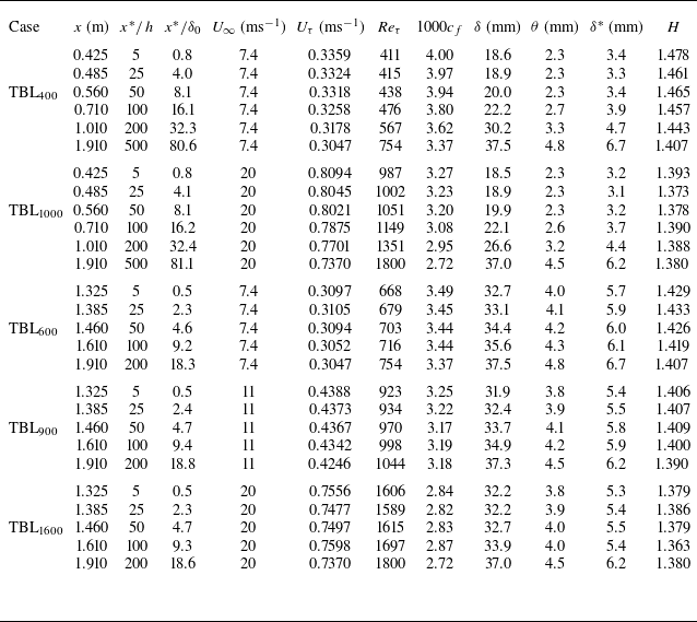


 Open access