





1. Introduction
The promise of the stellarator (Spitzer Jr. Reference Spitzer1958; Boozer Reference Boozer1998; Helander Reference Helander2014) as a means to achieving controlled magnetic confinement fusion has spurred activity in recent years (see, for instance, Parra Diaz et al. Reference Parra2024 and Warmer et al. Reference Warmer2024), with a particular focus on optimisation, i.e. finding the appropriate shape of the magnetic fields to support sufficient confinement of the plasma (Mynick Reference Mynick2006), and other desirable properties. Many shapes can be discarded at the outset due to their lack of sufficient particle confinement, and it is therefore appropriate to specialise to particular subclasses of configurations that confine particles by design. In this paper we are concerned with one such family, namely, quasi-isodynamic (QI) stellarators (Cary & Shasharina Reference Cary and Shasharina1997; Gori, Lotz & Nührenberg Reference Gori, Lotz and Nührenberg1997; Helander & Nührenberg Reference Helander and Nührenberg2009; Nührenberg 2010).
Quasi-isodynamic stellarators are defined as magnetic fields with nested flux surfaces with the following two properties. First, they belong to the larger class of omnigeneous stellarators (Hall & McNamara Reference Hall and McNamara1975; Bernardin, Moses & Tataronis Reference Bernardin, Moses and Tataronis1986; Cary & Shasharina Reference Cary and Shasharina1997; Helander Reference Helander2014); i.e. they, by construction, confine all collisionless charged particle orbits (Northrop Reference Northrop1961; Littlejohn Reference Littlejohn1983; Blank Reference de Blank2004; Wesson Reference Wesson2011), through a carefully tailored magnetic field magnitude $|\boldsymbol{B}|$
(Boozer Reference Boozer1983; Nührenberg & Zille Reference Nührenberg and Zille1988; Cary & Shasharina Reference Cary and Shasharina1997; Parra et al. Reference Parra, Calvo, Helander and Landreman2015). Second, the contours of
$|\boldsymbol{B}|$
(Boozer Reference Boozer1983; Nührenberg & Zille Reference Nührenberg and Zille1988; Cary & Shasharina Reference Cary and Shasharina1997; Parra et al. Reference Parra, Calvo, Helander and Landreman2015). Second, the contours of $|\boldsymbol{B}|$
over flux surfaces are closed the poloidal way around the torus. The latter confers QI configurations some advantageous properties over other omnigenous configurations (especially the celebrated quasisymmetric configurations; see Boozer Reference Boozer1983; Nührenberg & Zille Reference Nührenberg and Zille1988; Burby, Kallinikos & MacKay Reference Burby, Kallinikos and MacKay2020; Rodríguez et al. Reference Rodríguez, Helander and Bhattacharjee2020). In particular, the reduced level of bootstrap current (Helander & Nührenberg Reference Helander and Nührenberg2009) and narrower particle orbits are key distinctions, making QI stellarators an attractive stellarator class.
$|\boldsymbol{B}|$
over flux surfaces are closed the poloidal way around the torus. The latter confers QI configurations some advantageous properties over other omnigenous configurations (especially the celebrated quasisymmetric configurations; see Boozer Reference Boozer1983; Nührenberg & Zille Reference Nührenberg and Zille1988; Burby, Kallinikos & MacKay Reference Burby, Kallinikos and MacKay2020; Rodríguez et al. Reference Rodríguez, Helander and Bhattacharjee2020). In particular, the reduced level of bootstrap current (Helander & Nührenberg Reference Helander and Nührenberg2009) and narrower particle orbits are key distinctions, making QI stellarators an attractive stellarator class.
Following the above definition, the search for QI configurations is generally conducted via numerical optimisation (Gori et al. Reference Gori, Lotz and Nührenberg1997; Mikhailov et al. Reference Mikhailov, Shafranov, Subbotin, Isaev, Nührenberg, Zille and Cooper2002; Goodman et al. Reference Goodman, Camacho Mata, Henneberg, Jorge, Landreman, Plunk, Smith, Mackenbach, Beidler and Helander2023; Sánchez et al. Reference Sánchez, Velasco, Calvo and Mulas2023; Dudt et al. Reference Dudt, Goodman, Conlin, Panici and Kolemen2024). A cost function that vanishes when the definition is met is required to guide navigation over the space of stellarator equilibria. This approach has proven successful in its many different iterations, providing in some cases entire collections of configurations of varying quality (Cadena et al. Reference Cadena2025). However, this process is far from perfect, as optimisation is a highly nonlinear procedure performed over a vast parameter space consisting of many non-physical hyperparameters (Laia, Jorge & Abreu Reference Laia, Jorge and Abreu2025). Thus, navigation of the space of possible QI configurations is hampered by the lack of a solid underlying structure to help guide and interpret its mysterious behaviour. In addition, QI optimisation, more than other classes, is highly dependent on initial conditions (Goodman et al. Reference Goodman, Camacho Mata, Henneberg, Jorge, Landreman, Plunk, Smith, Mackenbach, Beidler and Helander2023), and it is thus important to derive these in a systematic way.
The near-axis expansion model (Mercier Reference Mercier1964; Solov’ev & Shafranov Reference Solov’ev and Shafranov1970; Lortz & Nührenberg Reference Lortz and Nührenberg1976; Garren & Boozer Reference Garren and Boozer1991) has proved to be an invaluable tool to tackle many of these limitations. This framework describes stellarator equilibria through their asymptotic expansion in the distance from the magnetic axis, providing a simplified, yet powerful perspective on the space of configurations. The model has seen significant development for quasisymmetric stellarators (Jorge & Landreman Reference Jorge and Landreman2020; Landreman & Jorge Reference Landreman and Jorge2020; Landreman Reference Landreman2021; Rodríguez et al. Reference Rodríguez, Sengupta and Bhattacharjee2022, Reference Rodríguez, Sengupta and Bhattacharjee2023), contributing to the understanding of their configuration space and enabling the generation of large databases of configurations. Recent examples of these can be found in Landreman (Reference Landreman2022), Giuliani (Reference Giuliani2024), Giuliani, Rodríguez & Spivak (Reference Giuliani, Rodríguez and Spivak2025), which make direct use of the near-axis expansion. An equivalent development of the model has however lagged for QI stellarators. Only most recently, through a series of papers (Plunk, Landreman & Helander Reference Plunk, Landreman and Helander2019; Camacho Mata, Plunk & Jorge Reference Camacho Mata, Plunk and Jorge2022; Jorge et al. Reference Jorge, Plunk, Drevlak, Landreman, Lobsien, Camacho Mata and Helander2022; Camacho Mata & Plunk Reference Camacho Mata and Plunk2023; Rodríguez & Plunk Reference Rodríguez and Plunk2023; Rodríguez et al. Reference Rodríguez, Plunk and Jorge2025; Rodriguez & Plunk Reference Rodríguez, Plunk and Jorge2025; Plunk & Rodríguez Reference Plunk and Rodríguez2026), the QI side of the model has matured to the point where a first thorough attempt at the exploration of the space of QI configurations may be attempted on par with the quasisymmetric configurations.
In this paper we present a first-of-its-kind database of more than 800 000 approximately QI vacuum near-axis configurations. The database is generated and structured such that each configuration is uniquely defined by a handful of scalar choices. The resulting space of solutions, though vast, is therefore possible to thoroughly explore. The near-axis framework enables each configuration to be swiftly diagnosed within the framework taking many different physical properties into account (Rodriguez & Plunk Reference Rodríguez, Plunk and Jorge2025), including elements of magnetohydrodynamic (MHD) stability, neoclassical transport or coil complexity. In this paper we explore some of these physical properties in detail, characterising those configurations that excel in these aspects and drawing physical and practical insight from it. Statistical and modern machine learning tools are also introduced to aid with the analysis of such vast data. Besides the interest of the individual stellarator fields themselves, and underlying physical and practical insights gained from the analysis, this paper also establishes the infrastructure for future more sophisticated, extensive and detailed analysis.
2. Construction of database
We follow recently developed methodologies (Rodríguez & Plunk Reference Rodríguez and Plunk2023; Plunk & Rodríguez Reference Plunk and Rodríguez2026) to construct approximately QI stellarator fields to second order in the near-axis expansion. In this section, basic details of this solution are described, and we refer the reader for the relevant details to mainly Rodríguez et al. (Reference Rodríguez, Plunk and Jorge2025) and Plunk & Rodríguez (Reference Plunk and Rodríguez2026).
The near-axis expansion proceeds from zeroth to first to then second order, at each stage accumulating more detail in the input parameter space and the output solution space. At zeroth order in the expansion, we must specify the shape of the magnetic axis and the magnetic field strength along it. Following Plunk & Rodríguez (Reference Plunk and Rodríguez2026), we define the shape of the magnetic axis, $\boldsymbol{x}_0$
, by prescribing curvature,
$\boldsymbol{x}_0$
, by prescribing curvature, $\kappa$
, and torsion,
$\kappa$
, and torsion, $\tau$
, as functions of the arc length
$\tau$
, as functions of the arc length $\ell \in [0,2\pi )$
, and solving the Frenet–Serret (FS) equations (Frenet Reference Frenet1852; Animov Reference Animov2001),
$\ell \in [0,2\pi )$
, and solving the Frenet–Serret (FS) equations (Frenet Reference Frenet1852; Animov Reference Animov2001),
 \begin{equation} \frac {\text{d}\boldsymbol{x}_0}{\text{d}\ell }=\hat {\boldsymbol{t}},\quad \frac {\text{d}\hat {\boldsymbol{t}}}{\text{d}\ell }=\kappa \hat {\boldsymbol{\kappa }},\quad \frac {\text{d}\hat {\boldsymbol{\kappa }}}{\text{d}\ell }=-\kappa \hat {\boldsymbol{t}} + \tau \hat {\boldsymbol{\tau }},\quad \frac {\text{d}\hat {\boldsymbol{\tau }}}{\text{d}\ell }=-\tau \hat {\boldsymbol{\kappa }}, \end{equation}
where $\hat {\boldsymbol{t}}$
is the tangent and
$\hat {\boldsymbol{t}}$
is the tangent and $(\hat {\boldsymbol{\kappa }},\hat {\boldsymbol{\tau }})$
are normal and binormal unit vectors. This approach to defining the curve enables direct control of the curvature and torsion, central ingredients in the near-axis framework. Thanks to this, we can easily impose two flattening points (of zero curvature) within each field period to comply with the requirements of a single-well QI field (Plunk et al. Reference Plunk, Landreman and Helander2019). To have a smooth framing of the curve, we must allow curvature to be negative to be a smooth function, resulting upon integration of (2.1) in the signed FS frame (Plunk et al. Reference Plunk, Landreman and Helander2019; Camacho Mata & Plunk Reference Camacho Mata and Plunk2023; Rodríguez et al. Reference Rodríguez, Plunk and Jorge2025). To ensure that a curve defined this way is properly closed, the curvature and torsion must be left some degrees of freedom to tweak, as detailed in Plunk & Rodríguez (Reference Plunk and Rodríguez2026). To accommodate these necessities, we parametrise curvature and torsion as
$(\hat {\boldsymbol{\kappa }},\hat {\boldsymbol{\tau }})$
are normal and binormal unit vectors. This approach to defining the curve enables direct control of the curvature and torsion, central ingredients in the near-axis framework. Thanks to this, we can easily impose two flattening points (of zero curvature) within each field period to comply with the requirements of a single-well QI field (Plunk et al. Reference Plunk, Landreman and Helander2019). To have a smooth framing of the curve, we must allow curvature to be negative to be a smooth function, resulting upon integration of (2.1) in the signed FS frame (Plunk et al. Reference Plunk, Landreman and Helander2019; Camacho Mata & Plunk Reference Camacho Mata and Plunk2023; Rodríguez et al. Reference Rodríguez, Plunk and Jorge2025). To ensure that a curve defined this way is properly closed, the curvature and torsion must be left some degrees of freedom to tweak, as detailed in Plunk & Rodríguez (Reference Plunk and Rodríguez2026). To accommodate these necessities, we parametrise curvature and torsion as
 \begin{align} \kappa & = 2\kappa _1\sin ^u\left (\frac {N\ell }{2}\right )\cos ^v\left (\frac {N\ell }{2}\right )\left [1+\sum _{n=2}^{N_\kappa }n\kappa _{n}\cos [(n-1)N\ell ]\right ], \end{align}
 \begin{align} \tau & = \tau _0+\sum _{n=1}^{N_\tau } \tau _{cn}\cos (n N \ell ), \end{align}
where $N\in \mathbb{N}^+$
is the number of field periods and we choose
$N\in \mathbb{N}^+$
is the number of field periods and we choose $u=2$
and
$u=2$
and $v=3$
. The parameters
$v=3$
. The parameters $\{\tau _0,\tau _{cn},\kappa _n\}$
can be thought of as the coefficients of a Fourier series, thus encompasing a larger space of functions for larger
$\{\tau _0,\tau _{cn},\kappa _n\}$
can be thought of as the coefficients of a Fourier series, thus encompasing a larger space of functions for larger $N_\kappa$
and
$N_\kappa$
and $N_\tau$
. For the purpose of the construction in this paper, we choose
$N_\tau$
. For the purpose of the construction in this paper, we choose $N_\tau =N_\kappa =2$
; that is, the set of coefficients is
$N_\tau =N_\kappa =2$
; that is, the set of coefficients is $\{\kappa _1,\kappa _2,\tau _0,\tau _{c1},\tau _{c2}\}$
. Of these coefficients, for
$\{\kappa _1,\kappa _2,\tau _0,\tau _{c1},\tau _{c2}\}$
. Of these coefficients, for $N\geqslant 2$
configurations,
$N\geqslant 2$
configurations, $\kappa _1$
and
$\kappa _1$
and $\tau _0$
are self-consistently found to ensure closure of the curve (Plunk & Rodríguez Reference Plunk and Rodríguez2026, § 2.2). The
$\tau _0$
are self-consistently found to ensure closure of the curve (Plunk & Rodríguez Reference Plunk and Rodríguez2026, § 2.2). The $N=1$
case is special and it requires four free parameters, leaving only
$N=1$
case is special and it requires four free parameters, leaving only $\tau _0$
as input (Plunk & Rodríguez Reference Plunk and Rodríguez2026, § 2.1).
$\tau _0$
as input (Plunk & Rodríguez Reference Plunk and Rodríguez2026, § 2.1).
The curvature has flattening points at maxima and minima of order $u=2$
and
$u=2$
and $v=3$
, respectively (the order of the first non-zero term in the expansion of
$v=3$
, respectively (the order of the first non-zero term in the expansion of $\kappa$
in
$\kappa$
in $\ell$
at such points). The order of the zero at the bottom,
$\ell$
at such points). The order of the zero at the bottom, $v$
, is chosen to be odd to comply with QI (Plunk et al. Reference Plunk, Landreman and Helander2019; Rodríguez & Plunk Reference Rodríguez and Plunk2023). The choice of
$v$
, is chosen to be odd to comply with QI (Plunk et al. Reference Plunk, Landreman and Helander2019; Rodríguez & Plunk Reference Rodríguez and Plunk2023). The choice of $u$
is made consistent with a
$u$
is made consistent with a $1/2$
helicity (Camacho Mata & Plunk Reference Camacho Mata and Plunk2023; Rodríguez et al. Reference Rodríguez, Plunk and Jorge2025, Appendix A) field (see Appendix E).
$1/2$
helicity (Camacho Mata & Plunk Reference Camacho Mata and Plunk2023; Rodríguez et al. Reference Rodríguez, Plunk and Jorge2025, Appendix A) field (see Appendix E).
The magnetic field strength is taken to have the form
 \begin{equation} B_0 = 1 + \varDelta \left [(1 + \lambda _B)\cos (N \ell ) + \left (\frac {1}{4} - 2 \lambda _B\right ) \cos (2 N \ell ) - \lambda _B \cos (3 N \ell )\right ]\!. \end{equation}
Such choice has $B_0'' = 0$
at field minima, suitable to promote MHD stability (Plunk et al. Reference Plunk, Drevlak, Rodriguez, Babin, Goodman and Hindenlang2024; Rodríguez et al. Reference Rodríguez, Helander and Goodman2024). The choice of
$B_0'' = 0$
at field minima, suitable to promote MHD stability (Plunk et al. Reference Plunk, Drevlak, Rodriguez, Babin, Goodman and Hindenlang2024; Rodríguez et al. Reference Rodríguez, Helander and Goodman2024). The choice of $v=3$
for the curvature is directly linked to this `flattened’ minimum, needed to avoid introducing QI-breaking defects in
$v=3$
for the curvature is directly linked to this `flattened’ minimum, needed to avoid introducing QI-breaking defects in $|\boldsymbol{B}|$
(Rodríguez & Plunk Reference Rodríguez and Plunk2023). In addition, the model for
$|\boldsymbol{B}|$
(Rodríguez & Plunk Reference Rodríguez and Plunk2023). In addition, the model for $B_0$
includes additional shaping parameters in the form of a mirror ratio,
$B_0$
includes additional shaping parameters in the form of a mirror ratio, $\varDelta = (B_0(0)-B_0(\pi /N))/2$
, and
$\varDelta = (B_0(0)-B_0(\pi /N))/2$
, and $\lambda _B$
, which controls the width of the well.
$\lambda _B$
, which controls the width of the well.
At first order in the construction we have freedom to specify the elliptical shape of the cross-sections in the FS frame. We construct the ellipticity (i.e. the ratio of major to minor axes of the ellipses) as a function of $\varphi$
, the toroidal Boozer angle, in terms of an auxiliary function
$\varphi$
, the toroidal Boozer angle, in terms of an auxiliary function $\rho =\rho (\varphi )$
(Plunk & Rodríguez Reference Plunk and Rodríguez2026):
$\rho =\rho (\varphi )$
(Plunk & Rodríguez Reference Plunk and Rodríguez2026):
 \begin{align} E(\varphi ) &= \frac {1}{2}\left (\rho + \sqrt {\rho ^2-4}\right )\!. \end{align}
The even function $\rho$
is given by
$\rho$
is given by
 \begin{equation} \rho = \rho _0 + \rho _1 \cos (N \varphi ) + \rho _2 \cos (2 N \varphi ), \end{equation}
where $\rho _0$
,
$\rho _0$
, $\rho _1$
and
$\rho _1$
and $\rho _2$
are free constants to be chosen. By controlling
$\rho _2$
are free constants to be chosen. By controlling $\rho$
, large elongation of flux surfaces can be prevented, avoiding the natural bias of QI fields. The drawback is that, in actuality, not all choices of parameters
$\rho$
, large elongation of flux surfaces can be prevented, avoiding the natural bias of QI fields. The drawback is that, in actuality, not all choices of parameters $\{\rho _n\}$
result in a valid solution through first order in the near-axis expansion (Plunk & Rodríguez Reference Plunk and Rodríguez2026, § 3.1), not even when
$\{\rho _n\}$
result in a valid solution through first order in the near-axis expansion (Plunk & Rodríguez Reference Plunk and Rodríguez2026, § 3.1), not even when $\rho \geqslant 2$
is satisfied. Thus, we must check the construction a posteriori to populate our database with valid first-order configurations.
$\rho \geqslant 2$
is satisfied. Thus, we must check the construction a posteriori to populate our database with valid first-order configurations.
The second order that completes the description of any configuration in our near-axis framework requires additional shaping inputs. Instead of including additional parameters that describe shaping, we follow the work in Rodriguez & Plunk (Reference Rodríguez, Plunk and Jorge2025) and consider, associated to each first-order choice, a whole family of minimally shaped configurations with different values of vacuum magnetic well, $W$
(Rodriguez & Plunk Reference Rodríguez, Plunk and Jorge2025, § 6). We shall often represent each of these families by its marginal representative,
$W$
(Rodriguez & Plunk Reference Rodríguez, Plunk and Jorge2025, § 6). We shall often represent each of these families by its marginal representative, $W=0$
, unless otherwise stated.
$W=0$
, unless otherwise stated.
Together, the free constants determining the functions $B_0$
,
$B_0$
, $\kappa$
,
$\kappa$
, $\tau$
and
$\tau$
and $\rho$
above, alongside
$\rho$
above, alongside $N$
, uniquely define then a marginally stable vacuum configuration. We define the input features to be minimal, unique set of input scalars
$N$
, uniquely define then a marginally stable vacuum configuration. We define the input features to be minimal, unique set of input scalars $\{\tau _{c1},\tau _{c2},$ $\kappa _2,\rho _0,\rho _1,\rho _2,\varDelta ,\lambda _B\}$
. The case of
$\kappa _2,\rho _0,\rho _1,\rho _2,\varDelta ,\lambda _B\}$
. The case of $N=1$
is special (due to the role of
$N=1$
is special (due to the role of $\tau _0$
) and we shall generally treat this case separately.
$\tau _0$
) and we shall generally treat this case separately.
With the prescription detailed above, we explicitly construct a database of more than 800 000 vacuum, approximately QI stellarators, with half-helicity and flattening class $(2,3)$
. To populate such a database, we scan the input features over a rectangular domain in regular increments.Footnote
1
The parameter domains and sampling is detailed in table 4 of Appendix A. These sampling domains must take into account the natural boundaries associated to each of the features. For instance, the solutions to the near-axis equations fails to exist when
$(2,3)$
. To populate such a database, we scan the input features over a rectangular domain in regular increments.Footnote
1
The parameter domains and sampling is detailed in table 4 of Appendix A. These sampling domains must take into account the natural boundaries associated to each of the features. For instance, the solutions to the near-axis equations fails to exist when $\rho$
is too low (Plunk & Rodríguez Reference Plunk and Rodríguez2026), which sets a lower bound on the minimal achievable elongation. Such limits are also present on the construction of the axis curves, which to comply with the desired helicity, cease to exist for large values of torsion. This sets an upper bound on parameters such as
$\rho$
is too low (Plunk & Rodríguez Reference Plunk and Rodríguez2026), which sets a lower bound on the minimal achievable elongation. Such limits are also present on the construction of the axis curves, which to comply with the desired helicity, cease to exist for large values of torsion. This sets an upper bound on parameters such as $\tau _{c1}$
(see figure 3 in Plunk & Rodríguez Reference Plunk and Rodríguez2026). Pushing the parameters to these extremes in the scan ensures that we are able to explore the full range of possible geometries captured within our model. Not every configuration constructed from such a scan can however be kept and archived in the database, only those that satisfy (i) closure of the axis curve, and (ii) periodicity and realness of the first-order solution of the
$\tau _{c1}$
(see figure 3 in Plunk & Rodríguez Reference Plunk and Rodríguez2026). Pushing the parameters to these extremes in the scan ensures that we are able to explore the full range of possible geometries captured within our model. Not every configuration constructed from such a scan can however be kept and archived in the database, only those that satisfy (i) closure of the axis curve, and (ii) periodicity and realness of the first-order solution of the $\sigma$
equation (Rodríguez et al. Reference Giuliani, Rodríguez and Spivak2025, equation (2.5); Plunk & Rodríguez Reference Plunk and Rodríguez2026, equation (3.1)) make the cut. Once the collection of configurations has been generated, their physical properties are assessed within the near-axis framework following Rodriguez & Plunk (Reference Rodríguez, Plunk and Jorge2025), Landreman & Jorge (Reference Landreman and Jorge2020), Landreman (Reference Landreman2021) and Rodríguez et al. (Reference Rodríguez, Helander and Goodman2024).
$\sigma$
equation (Rodríguez et al. Reference Giuliani, Rodríguez and Spivak2025, equation (2.5); Plunk & Rodríguez Reference Plunk and Rodríguez2026, equation (3.1)) make the cut. Once the collection of configurations has been generated, their physical properties are assessed within the near-axis framework following Rodriguez & Plunk (Reference Rodríguez, Plunk and Jorge2025), Landreman & Jorge (Reference Landreman and Jorge2020), Landreman (Reference Landreman2021) and Rodríguez et al. (Reference Rodríguez, Helander and Goodman2024).
3. General statistical and physical features of the QI database
The resulting database of near-axis QI configurations constructed following the prescription detailed in the previous section is made up of more than 800 000 different fields. There is no hope in studying the set on a one-by-one basis; a more practical, statistical approach to analysing the dataset is required. In this paper we analyse the database by examining the behaviour of select physical properties across it. The dataset exhibits substantial variability in these properties, with many configurations showing unpractical values in many of these regards. Identifying and characterising the features associated with the best-performing configurations provides valuable insights and shall be the focus of the analysis. To this end, we employ both descriptive statistical analyses and machine learning techniques, a detailed account of which is provided in Appendix B. We choose to focus here, for the most part separately, on elements of the field shaping complexity, MHD stability, maximum- $\mathcal{J}$
ness, neoclassical transport and finite
$\mathcal{J}$
ness, neoclassical transport and finite $\beta$
sensitivity. A more comprehensive exploration of ‘trade-offs’ between these properties, i.e. involving multivariate considerations, is reserved for future work.
$\beta$
sensitivity. A more comprehensive exploration of ‘trade-offs’ between these properties, i.e. involving multivariate considerations, is reserved for future work.
3.1. Magnetic gradient scale, $L_{{\boldsymbol{\nabla }\kern-1.2pt\boldsymbol{B}}}$

Each configuration in the database represents a different vacuum stellarator field. To physically sustain any of these magnetic fields, an appropriate arrangement of electric currents around the torus (electromagnetic coils) must be devised. In a reactor, it is desirable to place such coils sufficiently far from the fusing plasma, so that breeding blankets and neutron shielding may be fitted in between. However, there is an inherent cost to positioning coils far. The fine detail of the fields generated by coils, especially those with strong spatial variation, decay away from their generating currents. Thus, there is an inherent trade-off between coil distance and complexity, and it effectively becomes impossible to faithfully generate a given stellarator field at a sufficiently large distance. The $L_{{\boldsymbol{\nabla }\kern-1.2pt\boldsymbol{B}}}$
scalar measure is an attempt at describing this field-associated underlying scale.
$L_{{\boldsymbol{\nabla }\kern-1.2pt\boldsymbol{B}}}$
scalar measure is an attempt at describing this field-associated underlying scale.
We define the magnetic gradient scale, $L_{{\boldsymbol{\nabla }\kern-1.2pt\boldsymbol{B}}}$
, as
$L_{{\boldsymbol{\nabla }\kern-1.2pt\boldsymbol{B}}}$
, as
 \begin{equation} L_{{\boldsymbol{\nabla }\kern-1.2pt\boldsymbol{B}}}=\mathrm{min}\left [\frac {2B}{\|{\boldsymbol{\nabla }\kern-2.1pt\boldsymbol{B}}\|^2}\right ]\!, \end{equation}
following the original work of Landreman (Reference Landreman2021, equation (3.1)), and later explorations by Kappel, Landreman & Malhotra (Reference Kappel, Landreman and Malhotra2024). The minimum is meant to be computed over some selected flux surface, so that $L_{\boldsymbol{\nabla }\kern-1.2pt\boldsymbol{B}}$
may be interpreted as a proxy for how close coils need to be placed to said surface. To make sense of its magnitude, we normalise
$L_{\boldsymbol{\nabla }\kern-1.2pt\boldsymbol{B}}$
may be interpreted as a proxy for how close coils need to be placed to said surface. To make sense of its magnitude, we normalise $L_{{\boldsymbol{\nabla }\kern-1.2pt\boldsymbol{B}}}$
to the effective major radii of the configurations, defined as the length of the axis over
$L_{{\boldsymbol{\nabla }\kern-1.2pt\boldsymbol{B}}}$
to the effective major radii of the configurations, defined as the length of the axis over $2\pi$
. Thus, ‘better’ configurations will present larger values of
$2\pi$
. Thus, ‘better’ configurations will present larger values of $L_{{\boldsymbol{\nabla }\kern-1.2pt\boldsymbol{B}}}$
, which we may interpret as an inverse aspect ratio of the coil set.
$L_{{\boldsymbol{\nabla }\kern-1.2pt\boldsymbol{B}}}$
, which we may interpret as an inverse aspect ratio of the coil set.
Within the near-axis framework, we compute $L_{{\boldsymbol{\nabla }\kern-1.2pt\boldsymbol{B}}}$
using the asymptotic form of (3.1), originally derived in Landreman (Reference Landreman2021, equation (3.11)) for a general magnetic field. To leading order, the gradient
$L_{{\boldsymbol{\nabla }\kern-1.2pt\boldsymbol{B}}}$
using the asymptotic form of (3.1), originally derived in Landreman (Reference Landreman2021, equation (3.11)) for a general magnetic field. To leading order, the gradient $\|{\boldsymbol{\nabla }\kern-2.1pt\boldsymbol{B}}\|$
is determined by the axis and elliptical cross-section shapes (i.e. zeroth and first orders in the expansion), whose toroidal inhomogeneity makes it a function of the toroidal angle
$\|{\boldsymbol{\nabla }\kern-2.1pt\boldsymbol{B}}\|$
is determined by the axis and elliptical cross-section shapes (i.e. zeroth and first orders in the expansion), whose toroidal inhomogeneity makes it a function of the toroidal angle $\varphi$
.
$\varphi$
.
Other field scales could also be defined (most notably $L_{\boldsymbol{\nabla }\kern-0.9pt{\boldsymbol{\nabla }\kern-1.2pt\boldsymbol{B}}}$
(Landreman Reference Landreman2021) that include elements of second order and, thus, radial extent) and used as proxies. Ultimately, a highest fidelity description would necessitate an explicit coil construction (see, for instance, Giuliani et al. (Reference Giuliani, Wechsung, Cerfon, Stadler and Landreman2022)). Without going into the complexities of these measures, and noting that the database can be a good test bed ground for them, we opt for the simplest proxy in
$L_{\boldsymbol{\nabla }\kern-0.9pt{\boldsymbol{\nabla }\kern-1.2pt\boldsymbol{B}}}$
(Landreman Reference Landreman2021) that include elements of second order and, thus, radial extent) and used as proxies. Ultimately, a highest fidelity description would necessitate an explicit coil construction (see, for instance, Giuliani et al. (Reference Giuliani, Wechsung, Cerfon, Stadler and Landreman2022)). Without going into the complexities of these measures, and noting that the database can be a good test bed ground for them, we opt for the simplest proxy in $L_{{\boldsymbol{\nabla }\kern-1.2pt\boldsymbol{B}}}$
, backing its relevance on the evidence of Kappel et al. (Reference Kappel, Landreman and Malhotra2024).
$L_{{\boldsymbol{\nabla }\kern-1.2pt\boldsymbol{B}}}$
, backing its relevance on the evidence of Kappel et al. (Reference Kappel, Landreman and Malhotra2024).
3.1.1. General statistical description
The scalar $L_{{\boldsymbol{\nabla }\kern-1.2pt\boldsymbol{B}}}$
exhibits an immediately evident trend across the database: stellarators with a lower number of field periods,
$L_{{\boldsymbol{\nabla }\kern-1.2pt\boldsymbol{B}}}$
exhibits an immediately evident trend across the database: stellarators with a lower number of field periods, $N$
, favour longer field scales (see figure 1). Stellarators with
$N$
, favour longer field scales (see figure 1). Stellarators with $N=1,\,2$
can exhibit values as low as
$N=1,\,2$
can exhibit values as low as $L_{{\boldsymbol{\nabla }\kern-1.2pt\boldsymbol{B}}}\sim 0.4$
, that is, coils with as low an aspect ratio as
$L_{{\boldsymbol{\nabla }\kern-1.2pt\boldsymbol{B}}}\sim 0.4$
, that is, coils with as low an aspect ratio as $A\sim 2$
. To put these values in context, we may compare them to the survey in Kappel et al. (Reference Kappel, Landreman and Malhotra2024, figure 7). The comparison to
$A\sim 2$
. To put these values in context, we may compare them to the survey in Kappel et al. (Reference Kappel, Landreman and Malhotra2024, figure 7). The comparison to $L_{{\boldsymbol{\nabla }\kern-1.2pt\boldsymbol{B}}}$
values of other configurations must however be made with some words of caution. The near-axis
$L_{{\boldsymbol{\nabla }\kern-1.2pt\boldsymbol{B}}}$
values of other configurations must however be made with some words of caution. The near-axis $L_{{\boldsymbol{\nabla }\kern-1.2pt\boldsymbol{B}}}$
should be interpreted as a distance from the axis of the stellarator to coils, and not from the outermost flux surface of a finite aspect ratio configuration; that is, some sort of upper bound.Footnote
2
With this in mind, and applying the necessary spatial scaling, the lowest
$L_{{\boldsymbol{\nabla }\kern-1.2pt\boldsymbol{B}}}$
should be interpreted as a distance from the axis of the stellarator to coils, and not from the outermost flux surface of a finite aspect ratio configuration; that is, some sort of upper bound.Footnote
2
With this in mind, and applying the necessary spatial scaling, the lowest $L_{{\boldsymbol{\nabla }\kern-1.2pt\boldsymbol{B}}}$
values in the database correspond to
$L_{{\boldsymbol{\nabla }\kern-1.2pt\boldsymbol{B}}}$
values in the database correspond to $L_{{\boldsymbol{\nabla }\kern-1.2pt\boldsymbol{B}}}^\star \sim 7$
, matching the best-performing configurations in that work. It is no coincidence that these best-performing configurations do also correspond to
$L_{{\boldsymbol{\nabla }\kern-1.2pt\boldsymbol{B}}}^\star \sim 7$
, matching the best-performing configurations in that work. It is no coincidence that these best-performing configurations do also correspond to $N=1$
QI stellarators.
$N=1$
QI stellarators.
This improved behaviour at lower $N$
translates also to an increased number of configurations found above any reasonable realistic threshold. We take as a reference value
$N$
translates also to an increased number of configurations found above any reasonable realistic threshold. We take as a reference value $L_{{\boldsymbol{\nabla }\kern-1.2pt\boldsymbol{B}}}=0.25$
, which would amount to a distance of approximately 1.5 m from the plasma to the coils (in the ballpark of the needed space for various components in a fusion power plant; Beidler et al. Reference Beidler2001) for an aspect ratio 10,
$L_{{\boldsymbol{\nabla }\kern-1.2pt\boldsymbol{B}}}=0.25$
, which would amount to a distance of approximately 1.5 m from the plasma to the coils (in the ballpark of the needed space for various components in a fusion power plant; Beidler et al. Reference Beidler2001) for an aspect ratio 10, $R\sim 10\,\text{m}$
configuration. Setting a threshold for the analysis aligns with the notion of requiring a certain absolute physical plasma–coil distance to fit whichever elements are necessary (blanket, shielding, etc.). In this case, 96 % of the
$R\sim 10\,\text{m}$
configuration. Setting a threshold for the analysis aligns with the notion of requiring a certain absolute physical plasma–coil distance to fit whichever elements are necessary (blanket, shielding, etc.). In this case, 96 % of the $N=1$
population exceeds the threshold, 56 % for
$N=1$
population exceeds the threshold, 56 % for $N=2$
and merely a per cent for
$N=2$
and merely a per cent for $N=6$
(see the distributions in figure 1). This implies the need of larger aspect ratios for the practical realisation of larger
$N=6$
(see the distributions in figure 1). This implies the need of larger aspect ratios for the practical realisation of larger $N$
stellarators.
$N$
stellarators.
The shrinking of the $L_{{\boldsymbol{\nabla }\kern-1.2pt\boldsymbol{B}}}$
scale with field period number is expected from a purely geometric perspective. All other things being equal, a larger number of field periods requires any existing variation of the field to be packed into an increasingly narrower sector of the stellarator. Following this simple argument, we expect a linear scaling
$L_{{\boldsymbol{\nabla }\kern-1.2pt\boldsymbol{B}}}$
scale with field period number is expected from a purely geometric perspective. All other things being equal, a larger number of field periods requires any existing variation of the field to be packed into an increasingly narrower sector of the stellarator. Following this simple argument, we expect a linear scaling $L_{{\boldsymbol{\nabla }\kern-1.2pt\boldsymbol{B}}}\propto 1/N$
. The dependence seen in the database is however weaker (especially at lower
$L_{{\boldsymbol{\nabla }\kern-1.2pt\boldsymbol{B}}}\propto 1/N$
. The dependence seen in the database is however weaker (especially at lower $N$
; see figure 1) and although
$N$
; see figure 1) and although $N=1$
remains the best-performing, excellent candidates may also be found for a larger number of field periods. We show the configurations with the largest value of
$N=1$
remains the best-performing, excellent candidates may also be found for a larger number of field periods. We show the configurations with the largest value of $L_{{\boldsymbol{\nabla }\kern-1.2pt\boldsymbol{B}}}$
for each field period number in figure 1(b).
$L_{{\boldsymbol{\nabla }\kern-1.2pt\boldsymbol{B}}}$
for each field period number in figure 1(b).
Behaviour of $L_{{\boldsymbol{\nabla }\kern-1.2pt\boldsymbol{B}}}$
across different field periods
$L_{{\boldsymbol{\nabla }\kern-1.2pt\boldsymbol{B}}}$
across different field periods $N$
. (a) Dependence of the maximum and mean value of
$N$
. (a) Dependence of the maximum and mean value of $L_{{\boldsymbol{\nabla }\kern-1.2pt\boldsymbol{B}}}$
as a function of the number of field periods
$L_{{\boldsymbol{\nabla }\kern-1.2pt\boldsymbol{B}}}$
as a function of the number of field periods $N$
in the database. Reference scalings are given as dotted lines and the distribution of the configurations as violin plots. (b) Rendering of the 3D finite aspect ratio flux surface of
$N$
in the database. Reference scalings are given as dotted lines and the distribution of the configurations as violin plots. (b) Rendering of the 3D finite aspect ratio flux surface of $L_{{\boldsymbol{\nabla }\kern-1.2pt\boldsymbol{B}}}$
maximising fields for each number of field periods in the database. As a result of the increased surface shaping with
$L_{{\boldsymbol{\nabla }\kern-1.2pt\boldsymbol{B}}}$
maximising fields for each number of field periods in the database. As a result of the increased surface shaping with $N$
, the finite-volume representation of the configurations are shown for increasingly higher aspect ratios. The locations of
$N$
, the finite-volume representation of the configurations are shown for increasingly higher aspect ratios. The locations of $B_{\mathrm{min}}$
and
$B_{\mathrm{min}}$
and $B_{\mathrm{max}}$
are indicated for the
$B_{\mathrm{max}}$
are indicated for the $N=1$
configuration, which has the largest value of
$N=1$
configuration, which has the largest value of $L_{{\boldsymbol{\nabla }\kern-1.2pt\boldsymbol{B}}}$
of all configurations (see table 6).
$L_{{\boldsymbol{\nabla }\kern-1.2pt\boldsymbol{B}}}$
of all configurations (see table 6).

3.1.2. Geometric dependencies of
$L_{{\boldsymbol{\nabla }\kern-1.2pt\boldsymbol{B}}}$

It is interesting to ask what these large $L_{{\boldsymbol{\nabla }\kern-1.2pt\boldsymbol{B}}}$
configurations have in common and, in particular, which of their defining features (if any) consistently yield the observed behaviour. At a qualitative level, the configurations in figure 1(b) share a small off-the-plane excursion (relative to the
$L_{{\boldsymbol{\nabla }\kern-1.2pt\boldsymbol{B}}}$
configurations have in common and, in particular, which of their defining features (if any) consistently yield the observed behaviour. At a qualitative level, the configurations in figure 1(b) share a small off-the-plane excursion (relative to the $x$
-
$x$
- $y$
plane), yet an unevenly distributed torsion, particularly noticeable across the minimum of the magnetic field.
$y$
plane), yet an unevenly distributed torsion, particularly noticeable across the minimum of the magnetic field.
Statistical summary of feature dependence for $L_{{\boldsymbol{\nabla }\kern-1.2pt\boldsymbol{B}}}$
. This figure is representative of the input feature dependence of derived quantities employed in the analysis and discussion of the database, here exemplified by
$L_{{\boldsymbol{\nabla }\kern-1.2pt\boldsymbol{B}}}$
. This figure is representative of the input feature dependence of derived quantities employed in the analysis and discussion of the database, here exemplified by $L_{{\boldsymbol{\nabla }\kern-1.2pt\boldsymbol{B}}}$
. (a) Scatter plots illustrating any univariate dependence of
$L_{{\boldsymbol{\nabla }\kern-1.2pt\boldsymbol{B}}}$
. (a) Scatter plots illustrating any univariate dependence of $L_{{\boldsymbol{\nabla }\kern-1.2pt\boldsymbol{B}}}$
on the features
$L_{{\boldsymbol{\nabla }\kern-1.2pt\boldsymbol{B}}}$
on the features $\tau _{c1}$
and
$\tau _{c1}$
and $\tau _{c2}$
for the
$\tau _{c2}$
for the $N=2$
subset. (b) Summary of key statistical measures describing the dependence of
$N=2$
subset. (b) Summary of key statistical measures describing the dependence of $L_{{\boldsymbol{\nabla }\kern-1.2pt\boldsymbol{B}}}$
on input features. (b i) Linear correlation between the input features and
$L_{{\boldsymbol{\nabla }\kern-1.2pt\boldsymbol{B}}}$
on input features. (b i) Linear correlation between the input features and $L_{{\boldsymbol{\nabla }\kern-1.2pt\boldsymbol{B}}}$
. The different symbols indicate the Pearson and Spearman coefficients, while the colour distinguishes a different number of field periods. (bii) Nonlinear correlation coefficient, where the colour distinguishes a different number of field periods. (b iii) Friedman H-statistic where the size of the scatter indicates the significance of the measure compared with a null reference distribution and the colour represents a different numbers of field periods. The labels indicate which other feature they are most closely linked to. (b iv) Relative feature importance with symbols representing the PFI and cSAGE measures and the colour a different number of field periods. The values listed to the right next to the scatter indicate the coefficient of determination of a multivariate SVM model fitted to
$L_{{\boldsymbol{\nabla }\kern-1.2pt\boldsymbol{B}}}$
. The different symbols indicate the Pearson and Spearman coefficients, while the colour distinguishes a different number of field periods. (bii) Nonlinear correlation coefficient, where the colour distinguishes a different number of field periods. (b iii) Friedman H-statistic where the size of the scatter indicates the significance of the measure compared with a null reference distribution and the colour represents a different numbers of field periods. The labels indicate which other feature they are most closely linked to. (b iv) Relative feature importance with symbols representing the PFI and cSAGE measures and the colour a different number of field periods. The values listed to the right next to the scatter indicate the coefficient of determination of a multivariate SVM model fitted to $L_{{\boldsymbol{\nabla }\kern-1.2pt\boldsymbol{B}}}$
as a function of the input features.
$L_{{\boldsymbol{\nabla }\kern-1.2pt\boldsymbol{B}}}$
as a function of the input features.

A more quantitative analysis of such observations requires us to be more systematic with the approach to the problem. In that direction we separate the features associated to each configuration in the database into: input features (i.e. the minimal set of parameters uniquely describing configurations) and derived features (i.e. derived properties describing the configuration, such as $L_{{\boldsymbol{\nabla }\kern-1.2pt\boldsymbol{B}}}$
). The former constitutes the fundamental feature vector (following the standard machine learning nomenclature), which by virtue of the near-axis construction represents not just labels, but a precise physical description of the configurations: namely, their fundamental shape and field features. We will base our quantitative analysis on various statistical measures (detailed in Appendix B) focused on the role of these input features, which by virtue of the near-axis construction constitute a low-dimensional space.
$L_{{\boldsymbol{\nabla }\kern-1.2pt\boldsymbol{B}}}$
). The former constitutes the fundamental feature vector (following the standard machine learning nomenclature), which by virtue of the near-axis construction represents not just labels, but a precise physical description of the configurations: namely, their fundamental shape and field features. We will base our quantitative analysis on various statistical measures (detailed in Appendix B) focused on the role of these input features, which by virtue of the near-axis construction constitute a low-dimensional space.
Let us start the analysis of the influence of the input features on $L_{{\boldsymbol{\nabla }\kern-1.2pt\boldsymbol{B}}}$
by looking at linear correlations (see figure 2
b). The lack of a strong correlation (barring the special
$L_{{\boldsymbol{\nabla }\kern-1.2pt\boldsymbol{B}}}$
by looking at linear correlations (see figure 2
b). The lack of a strong correlation (barring the special $N=1$
case) reflects the lack of a monotonic relation with any of the input features (see figure 2
a), but not necessarily a complete disconnection. We therefore need to supplement the analysis with an alternative that relaxes the monotonicity assumption. We construct a nonlinear correlation measure (see Appendix B for details) based on the goodness of fit of a univariate nonlinear model. This measure (figure 2
b) unveils a significant non-monotonic dependence, highlighting details of the axis shape, with pre-eminence of
$N=1$
case) reflects the lack of a monotonic relation with any of the input features (see figure 2
a), but not necessarily a complete disconnection. We therefore need to supplement the analysis with an alternative that relaxes the monotonicity assumption. We construct a nonlinear correlation measure (see Appendix B for details) based on the goodness of fit of a univariate nonlinear model. This measure (figure 2
b) unveils a significant non-monotonic dependence, highlighting details of the axis shape, with pre-eminence of $\tau _{c2}$
(
$\tau _{c2}$
( $R^2\gtrsim 0.5$
across all different
$R^2\gtrsim 0.5$
across all different $N$
).
$N$
).
Despite the significance of the univariate description of $L_{{\boldsymbol{\nabla }\kern-1.2pt\boldsymbol{B}}}$
, any such isolated model fails to capture the whole complexity of the database. We need to consider the dependence on multiple features simultaneously. When we consider all input features simultaneously, even a simple support vector regression (SVR) (Schölkopf & Smola 2002; Hastie, Tibshirani & Friedman Reference Hastie, Tibishirani and Friedman2009, Chapter 12.3.6.) model for
$L_{{\boldsymbol{\nabla }\kern-1.2pt\boldsymbol{B}}}$
, any such isolated model fails to capture the whole complexity of the database. We need to consider the dependence on multiple features simultaneously. When we consider all input features simultaneously, even a simple support vector regression (SVR) (Schölkopf & Smola 2002; Hastie, Tibshirani & Friedman Reference Hastie, Tibishirani and Friedman2009, Chapter 12.3.6.) model for $L_{{\boldsymbol{\nabla }\kern-1.2pt\boldsymbol{B}}}$
can account for more than 95 % of the database variability (
$L_{{\boldsymbol{\nabla }\kern-1.2pt\boldsymbol{B}}}$
can account for more than 95 % of the database variability ( $R^2\gtrsim 0.95$
) without falling into overfitting (see details in Appendix B). Clearly, a multivariate description is more predictive, but does not unveil how much each feature contributes to predictions. To assess such relative importance, we use permutation feature importance (PFI) and conditional Shapley additive global importance (cSAGE) (see full details in Appendix B). Both measures (figure 2
b) corroborate the dominant role of torsion and
$R^2\gtrsim 0.95$
) without falling into overfitting (see details in Appendix B). Clearly, a multivariate description is more predictive, but does not unveil how much each feature contributes to predictions. To assess such relative importance, we use permutation feature importance (PFI) and conditional Shapley additive global importance (cSAGE) (see full details in Appendix B). Both measures (figure 2
b) corroborate the dominant role of torsion and $\tau _{c2}$
, in particular, providing them high scores.
$\tau _{c2}$
, in particular, providing them high scores.
The $\tau _{c1}$
parameter does also appear to be important, but its role appears to swing wildly between different
$\tau _{c1}$
parameter does also appear to be important, but its role appears to swing wildly between different $N$
. This variability can in part be explained by the interaction of
$N$
. This variability can in part be explained by the interaction of $\tau _{c1}$
with
$\tau _{c1}$
with $\tau _{c2}$
in the
$\tau _{c2}$
in the $L_{{\boldsymbol{\nabla }\kern-1.2pt\boldsymbol{B}}}$
prediction. To describe this feature dependence, we compute the Friedman H-statistic (see Appendix B), which provides a measure of how much of the prediction really requires simultaneous knowledge of both features. In the case of
$L_{{\boldsymbol{\nabla }\kern-1.2pt\boldsymbol{B}}}$
prediction. To describe this feature dependence, we compute the Friedman H-statistic (see Appendix B), which provides a measure of how much of the prediction really requires simultaneous knowledge of both features. In the case of $\tau _{c1}$
, figure 2(b) shows that approximately
$\tau _{c1}$
, figure 2(b) shows that approximately ${\sim}20\,\,\%$
of the behaviour requires the explicit involvement of both torsion features.
${\sim}20\,\,\%$
of the behaviour requires the explicit involvement of both torsion features.
3.1.3. Understanding the role of torsion
Although it is unsurprising that torsion plays a role in setting $L_{{\boldsymbol{\nabla }\kern-1.2pt\boldsymbol{B}}}$
, the relative unimportance of curvature may come as a surprise, as the gradients in
$L_{{\boldsymbol{\nabla }\kern-1.2pt\boldsymbol{B}}}$
, the relative unimportance of curvature may come as a surprise, as the gradients in $\|\boldsymbol{B}\|$
are controlled by curvature, and thus, we naturally expect it to contribute to setting the length scales relevant to the field.
$\|\boldsymbol{B}\|$
are controlled by curvature, and thus, we naturally expect it to contribute to setting the length scales relevant to the field.
An explanation of this observation necessitates a more precise consideration of the contributions to $L_{{\boldsymbol{\nabla }\kern-1.2pt\boldsymbol{B}}}$
at a theoretical level. In that direction, consider the leading asymptotic form of
$L_{{\boldsymbol{\nabla }\kern-1.2pt\boldsymbol{B}}}$
at a theoretical level. In that direction, consider the leading asymptotic form of $L_{{\boldsymbol{\nabla }\kern-1.2pt\boldsymbol{B}}}$
(Landreman Reference Landreman2021, equation (3.11)), written in the ideal QI limitFootnote
3
as
$L_{{\boldsymbol{\nabla }\kern-1.2pt\boldsymbol{B}}}$
(Landreman Reference Landreman2021, equation (3.11)), written in the ideal QI limitFootnote
3
as
 \begin{align} {\boldsymbol{\nabla }\kern-2.1pt\boldsymbol{B}}\approx \frac {B_0}{\ell '}\left (\frac {\bar {e}'}{2\bar {e}}-\frac {B_0'}{2B_0}\right )\hat {\boldsymbol{\kappa }}\hat {\boldsymbol{\kappa }} - \frac {B_0}{\ell '}\left (\frac {\bar {e}'}{2\bar {e}}+\frac {B_0'}{2B_0}\right )\hat {\boldsymbol{\tau }}\hat {\boldsymbol{\tau }} \nonumber \\[5pt] +\,B_0\tau (\hat {\boldsymbol{\kappa }}\hat {\boldsymbol{\tau }}-\hat {\boldsymbol{\tau }}\hat {\boldsymbol{\kappa }})+B_0\kappa (\hat {\boldsymbol{t}}\hat {\boldsymbol{\kappa }}+\hat {\boldsymbol{\kappa }}\hat {\boldsymbol{t}})+\frac {B_0'}{\ell '}\hat {\boldsymbol{t}}\hat {\boldsymbol{t}}. \end{align}
There are four physical sources of length scales in the field: the variation of the field strength along the axis ( $B_0'$
), the variation of elongation (
$B_0'$
), the variation of elongation ( $\bar {e}'$
),Footnote
4
the curvature (
$\bar {e}'$
),Footnote
4
the curvature ( $\kappa$
) and the torsion (
$\kappa$
) and the torsion ( $\tau$
). The main curvature term is directly related to the bending (
$\tau$
). The main curvature term is directly related to the bending ( $\hat {\boldsymbol{\kappa }}$
) of field lines (
$\hat {\boldsymbol{\kappa }}$
) of field lines ( $\hat {\boldsymbol{t}}$
), while the main torsion term clearly corresponds to twisting of the frame (
$\hat {\boldsymbol{t}}$
), while the main torsion term clearly corresponds to twisting of the frame ( $\hat {\boldsymbol{\tau }}\hat {\boldsymbol{\kappa }}-\hat {\boldsymbol{\kappa }}\hat {\boldsymbol{\tau }}$
). In practice, in the context of the database, we may focus on these two contributions to explain the behaviour of
$\hat {\boldsymbol{\tau }}\hat {\boldsymbol{\kappa }}-\hat {\boldsymbol{\kappa }}\hat {\boldsymbol{\tau }}$
). In practice, in the context of the database, we may focus on these two contributions to explain the behaviour of $L_{{\boldsymbol{\nabla }\kern-1.2pt\boldsymbol{B}}}$
. Both
$L_{{\boldsymbol{\nabla }\kern-1.2pt\boldsymbol{B}}}$
. Both $B_0'$
and
$B_0'$
and $\bar {e}'$
(which depends directly on
$\bar {e}'$
(which depends directly on $\tau$
and
$\tau$
and $\rho$
) can be largely treated as secondary so long as their variations are tamed, which the direct control of
$\rho$
) can be largely treated as secondary so long as their variations are tamed, which the direct control of $B_0$
and elongation in the construction enables.
$B_0$
and elongation in the construction enables.
Following (3.2), $\kappa$
and
$\kappa$
and $\tau$
contribute on equal footing to
$\tau$
contribute on equal footing to $\|{\boldsymbol{\nabla }\kern-2.1pt\boldsymbol{B}}\|$
. The difference in their roles can be traced to the fact that the omnigenous (or rather the pseudosymmetric; see Skovoroda (Reference Skovoroda2005)) requirement on the magnetic field constrains curvature in particular, forcing it to vanish at the maxima and minima of the magnetic field (Plunk et al. Reference Plunk, Landreman and Helander2019). The field gradient at these straight sections is thus uniquely set by torsion, whose value at the bottom we denote by
$\|{\boldsymbol{\nabla }\kern-2.1pt\boldsymbol{B}}\|$
. The difference in their roles can be traced to the fact that the omnigenous (or rather the pseudosymmetric; see Skovoroda (Reference Skovoroda2005)) requirement on the magnetic field constrains curvature in particular, forcing it to vanish at the maxima and minima of the magnetic field (Plunk et al. Reference Plunk, Landreman and Helander2019). The field gradient at these straight sections is thus uniquely set by torsion, whose value at the bottom we denote by $\check {\tau }$
. Away from the flattening points, curvature grows and the scale of the field is set by a combination of combining curvature and torsion that peaks somewhere half-way to the maximum.
$\check {\tau }$
. Away from the flattening points, curvature grows and the scale of the field is set by a combination of combining curvature and torsion that peaks somewhere half-way to the maximum.
Making a direct connection between these theoretical observations and the role played by the input features is highly non-trivial. A prime example of this is the relation of the input features to $\check {\tau }$
(or any other value of torsion around the axis), which requires knowledge of
$\check {\tau }$
(or any other value of torsion around the axis), which requires knowledge of $\tau _0$
after solving the axis closure problem, besides
$\tau _0$
after solving the axis closure problem, besides $\tau _{c1}$
and
$\tau _{c1}$
and $\tau _{c2}$
. It is then natural to set up a statistical analysis of the database with an extended feature vector that includes
$\tau _{c2}$
. It is then natural to set up a statistical analysis of the database with an extended feature vector that includes $\tau _0$
and
$\tau _0$
and $\kappa _1$
. We may go beyond and complement these with a plethora of other meaningful feature combinations (see a full account of these in Appendix B), including, for instance,
$\kappa _1$
. We may go beyond and complement these with a plethora of other meaningful feature combinations (see a full account of these in Appendix B), including, for instance, $\check {\tau }$
or the position of the maximum of curvature
$\check {\tau }$
or the position of the maximum of curvature $\ell _\kappa$
. A similar dependence question on
$\ell _\kappa$
. A similar dependence question on $L_{{\boldsymbol{\nabla }\kern-1.2pt\boldsymbol{B}}}$
could now be posed on this extended set of features. The problem is however significantly different from the original, as the features considered are no longer strongly independent. Adapting the analysis of the problem to this reality, we find it fitting to adopt the forward sequential feature selection (FSFS) (Whitney Reference Whitney1971). The importance of features in
$L_{{\boldsymbol{\nabla }\kern-1.2pt\boldsymbol{B}}}$
could now be posed on this extended set of features. The problem is however significantly different from the original, as the features considered are no longer strongly independent. Adapting the analysis of the problem to this reality, we find it fitting to adopt the forward sequential feature selection (FSFS) (Whitney Reference Whitney1971). The importance of features in $L_{{\boldsymbol{\nabla }\kern-1.2pt\boldsymbol{B}}}$
is defined by sequentially choosing (and ranking) features so as to maximise the goodness of a model for
$L_{{\boldsymbol{\nabla }\kern-1.2pt\boldsymbol{B}}}$
is defined by sequentially choosing (and ranking) features so as to maximise the goodness of a model for $L_{{\boldsymbol{\nabla }\kern-1.2pt\boldsymbol{B}}}$
fitted to a sequentially increasing number of features (see the details in Appendix B). The results are summarised in table 1.
$L_{{\boldsymbol{\nabla }\kern-1.2pt\boldsymbol{B}}}$
fitted to a sequentially increasing number of features (see the details in Appendix B). The results are summarised in table 1.
Dominant extended features for $L_{{\boldsymbol{\nabla }\kern-1.2pt\boldsymbol{B}}}$
. The table summarises the top selected features by FSFS on the extended features detailed in Appendix B. The numerical value represents the coefficient of determination
$L_{{\boldsymbol{\nabla }\kern-1.2pt\boldsymbol{B}}}$
. The table summarises the top selected features by FSFS on the extended features detailed in Appendix B. The numerical value represents the coefficient of determination $R^2$
of the
$R^2$
of the $L_{{\boldsymbol{\nabla }\kern-1.2pt\boldsymbol{B}}}$
model using the variable on that row alongside those above. The meaning of the various parameters in the table are presented in Appendix B:
$L_{{\boldsymbol{\nabla }\kern-1.2pt\boldsymbol{B}}}$
model using the variable on that row alongside those above. The meaning of the various parameters in the table are presented in Appendix B: $\hat {\tau },\check {\tau }$
is the torsion at
$\hat {\tau },\check {\tau }$
is the torsion at $B_{\mathrm{max}}$
and
$B_{\mathrm{max}}$
and $B_{\mathrm{min}}$
,
$B_{\mathrm{min}}$
, $\tau _{\mathrm{min}},\tau _{\mathrm{max}}$
are the minimum and maximum torsion, respectively,
$\tau _{\mathrm{min}},\tau _{\mathrm{max}}$
are the minimum and maximum torsion, respectively, $\sigma _\tau$
is the standard deviation of torsion and
$\sigma _\tau$
is the standard deviation of torsion and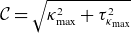 $\mathcal{C}=\sqrt {\kappa _{\mathrm{max}}^2+\tau _{\mathrm{\kappa _{\mathrm{max}}}}^2}$
, with
$\mathcal{C}=\sqrt {\kappa _{\mathrm{max}}^2+\tau _{\mathrm{\kappa _{\mathrm{max}}}}^2}$
, with $\kappa _{\mathrm{max}}$
the maximum curvature and
$\kappa _{\mathrm{max}}$
the maximum curvature and $\tau _{\mathrm{\kappa _{\mathrm{max}}}}$
the value of torsion there.
$\tau _{\mathrm{\kappa _{\mathrm{max}}}}$
the value of torsion there.

Analysis of torsion dependence of $L_{{\boldsymbol{\nabla }\kern-1.2pt\boldsymbol{B}}}$
. Panel (a) shows
$L_{{\boldsymbol{\nabla }\kern-1.2pt\boldsymbol{B}}}$
. Panel (a) shows $L_{{\boldsymbol{\nabla }\kern-1.2pt\boldsymbol{B}}}$
in the
$L_{{\boldsymbol{\nabla }\kern-1.2pt\boldsymbol{B}}}$
in the $N=4$
subset (light grey scatter) as a function of the value of torsion at the field minimum,
$N=4$
subset (light grey scatter) as a function of the value of torsion at the field minimum, $\check {\tau }$
, and the combination of torsion and curvature at the point where curvature is maximum,
$\check {\tau }$
, and the combination of torsion and curvature at the point where curvature is maximum, $\mathcal{C}$
. The black broken lines represent the two different predicted upper bounds for
$\mathcal{C}$
. The black broken lines represent the two different predicted upper bounds for $L_{{\boldsymbol{\nabla }\kern-1.2pt\boldsymbol{B}}}$
, illustrating the two limiting contributions indicated in the diagram (panel b). The behaviour of
$L_{{\boldsymbol{\nabla }\kern-1.2pt\boldsymbol{B}}}$
, illustrating the two limiting contributions indicated in the diagram (panel b). The behaviour of $\|{\boldsymbol{\nabla }\kern-2.1pt\boldsymbol{B}}\|$
in these two limits is exemplified for two example configurations (i) and (ii) in panel (a). Curvature and torsion are also shown for comparison.
$\|{\boldsymbol{\nabla }\kern-2.1pt\boldsymbol{B}}\|$
in these two limits is exemplified for two example configurations (i) and (ii) in panel (a). Curvature and torsion are also shown for comparison.

The most relevant features appear directly related to torsion, in agreement with the reduced input feature analysis. Remarkably, the statistical analysis points at the torsion at the field minimum to be of particular importance (describing ${\sim}80\,\%$
of the data variance), connecting directly to our preceding theoretical discussion. Figure 3 illustrates
${\sim}80\,\%$
of the data variance), connecting directly to our preceding theoretical discussion. Figure 3 illustrates $L_{{\boldsymbol{\nabla }\kern-1.2pt\boldsymbol{B}}}$
(for the
$L_{{\boldsymbol{\nabla }\kern-1.2pt\boldsymbol{B}}}$
(for the $N=4$
case) as a function of
$N=4$
case) as a function of $\check {\tau }$
, clearly showing that the value of the torsion at the field minimum sets an upper bound
$\check {\tau }$
, clearly showing that the value of the torsion at the field minimum sets an upper bound $L_{{\boldsymbol{\nabla }\kern-1.2pt\boldsymbol{B}}}\sim 1/\check {\tau }$
. Having an odd order of curvature at the field minimum forces a non-zero off-plane excursion of the axis, see Rodríguez et al. (Reference Giuliani, Rodríguez and Spivak2025, Appendix A) or Plunk & Rodríguez (Reference Plunk and Rodríguez2026, Appendix A), and thus, generally an indelible finite torsion in the neighbourhood of
$L_{{\boldsymbol{\nabla }\kern-1.2pt\boldsymbol{B}}}\sim 1/\check {\tau }$
. Having an odd order of curvature at the field minimum forces a non-zero off-plane excursion of the axis, see Rodríguez et al. (Reference Giuliani, Rodríguez and Spivak2025, Appendix A) or Plunk & Rodríguez (Reference Plunk and Rodríguez2026, Appendix A), and thus, generally an indelible finite torsion in the neighbourhood of $B_{\mathrm{min}}$
, unlike near the maximum. The contribution to
$B_{\mathrm{min}}$
, unlike near the maximum. The contribution to $\|{\boldsymbol{\nabla }\kern-2.1pt\boldsymbol{B}}\|$
is minimised there by keeping torsion spatially separated from curvature, and thus, this finite torsion through the minimum is the least detrimental form of torsion that sets a minimal scale for
$\|{\boldsymbol{\nabla }\kern-2.1pt\boldsymbol{B}}\|$
is minimised there by keeping torsion spatially separated from curvature, and thus, this finite torsion through the minimum is the least detrimental form of torsion that sets a minimal scale for $L_{{\boldsymbol{\nabla }\kern-1.2pt\boldsymbol{B}}}$
. This limiting torsion (i.e. local twist) around
$L_{{\boldsymbol{\nabla }\kern-1.2pt\boldsymbol{B}}}$
. This limiting torsion (i.e. local twist) around $B_{\mathrm{min}}$
aligns with the configurations of figure 1, especially clear for
$B_{\mathrm{min}}$
aligns with the configurations of figure 1, especially clear for $N=1$
.
$N=1$
.
The $N=1$
case is rather especial, in part because of its reduced range of input features (a single free parameter
$N=1$
case is rather especial, in part because of its reduced range of input features (a single free parameter $\tau _0$
is scanned instead of
$\tau _0$
is scanned instead of $\{\tau _{c1},\tau _{c2},\kappa _1\}$
). However,
$\{\tau _{c1},\tau _{c2},\kappa _1\}$
). However, $\check {\tau }$
remains to capture
$\check {\tau }$
remains to capture ${\sim}99.5\,\%$
of the data variance, even if it does not appear in table 1. This highlights an important caveat of FSFS: it may hide features of similar importance just because a similar amount of information is given by an already included feature. This is partly what occurs at larger
${\sim}99.5\,\%$
of the data variance, even if it does not appear in table 1. This highlights an important caveat of FSFS: it may hide features of similar importance just because a similar amount of information is given by an already included feature. This is partly what occurs at larger $N$
where the variation of the torsion along the axis,
$N$
where the variation of the torsion along the axis, $\sigma _\tau$
, overtakes
$\sigma _\tau$
, overtakes $\check {\tau }$
, even though the later remains highly important (
$\check {\tau }$
, even though the later remains highly important ( $R^2\gt 0.8$
). This shift might nevertheless indicate an increased struggle to keeping the value of torsion tamed elsewhere, driven by
$R^2\gt 0.8$
). This shift might nevertheless indicate an increased struggle to keeping the value of torsion tamed elsewhere, driven by $N$
.
$N$
.
This perspective, emphasising torsion at $B_{\mathrm{min}}$
, is however not complete, as it would suggest
$B_{\mathrm{min}}$
, is however not complete, as it would suggest $\check {\tau }\rightarrow 0$
to maximise
$\check {\tau }\rightarrow 0$
to maximise $L_{{\boldsymbol{\nabla }\kern-1.2pt\boldsymbol{B}}}$
, but figure 3 shows that this fails below some critical
$L_{{\boldsymbol{\nabla }\kern-1.2pt\boldsymbol{B}}}$
, but figure 3 shows that this fails below some critical $\check {\tau }$
value. In this limit the configurations are no longer limited by the field gradients at
$\check {\tau }$
value. In this limit the configurations are no longer limited by the field gradients at $B_{\mathrm{min}}$
, but instead a combination of curvature and torsion somewhere between
$B_{\mathrm{min}}$
, but instead a combination of curvature and torsion somewhere between $B_{\mathrm{min}}$
and
$B_{\mathrm{min}}$
and $B_{\mathrm{max}}$
(see
$B_{\mathrm{max}}$
(see $\|{\boldsymbol{\nabla }\kern-2.1pt\boldsymbol{B}}\|$
for configuration (ii) in figure 3). Such a combination mentioned in the theoretical discussion does also appear in the FSFS analysis in the form of
$\|{\boldsymbol{\nabla }\kern-2.1pt\boldsymbol{B}}\|$
for configuration (ii) in figure 3). Such a combination mentioned in the theoretical discussion does also appear in the FSFS analysis in the form of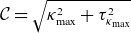 $\mathcal{C}=\sqrt {\kappa _{\mathrm{max}}^2+\tau _{\mathrm{\kappa _{\mathrm{max}}}}^2}$
. This combination serves indeed as an upper bound
$\mathcal{C}=\sqrt {\kappa _{\mathrm{max}}^2+\tau _{\mathrm{\kappa _{\mathrm{max}}}}^2}$
. This combination serves indeed as an upper bound $L_{{\boldsymbol{\nabla }\kern-1.2pt\boldsymbol{B}}}\sim 1/\mathcal{C}$
; see figure 3. Despite this clear role, the FSFS analysis only gives
$L_{{\boldsymbol{\nabla }\kern-1.2pt\boldsymbol{B}}}\sim 1/\mathcal{C}$
; see figure 3. Despite this clear role, the FSFS analysis only gives $\mathcal{C}$
a secondary role. Here
$\mathcal{C}$
a secondary role. Here $\check {\tau }$
appears to capture its behaviour to a good degree; after all, torsion and curvature are tightly linked.
$\check {\tau }$
appears to capture its behaviour to a good degree; after all, torsion and curvature are tightly linked.
The best configurations will therefore attempt to minimise both these features as much as possible. First, they will try to minimise torsion, being left with some remanent through $B_{\mathrm{min}}$
. Second, they will limit the peak curvature to the largest extent possible and spatially separate it from the torsion contribution. It is then expected (and observed) for curves of maximal
$B_{\mathrm{min}}$
. Second, they will limit the peak curvature to the largest extent possible and spatially separate it from the torsion contribution. It is then expected (and observed) for curves of maximal $L_{{\boldsymbol{\nabla }\kern-1.2pt\boldsymbol{B}}}$
to be rather flat, but retain a small off-the-plane excursion. Extreme elongation variations or a mirror ratio should also be avoided, but these issues are a lesser problem in practice.
$L_{{\boldsymbol{\nabla }\kern-1.2pt\boldsymbol{B}}}$
to be rather flat, but retain a small off-the-plane excursion. Extreme elongation variations or a mirror ratio should also be avoided, but these issues are a lesser problem in practice.
3.2. Critical aspect ratio of stabilised field,
$A_c^{\mathrm{mhd}}$

One of the key developments of Rodriguez & Plunk (Reference Rodríguez, Plunk and Jorge2025) was the possibility of constructing MHD stable near-axis fields with a minimum amount of shaping and without the need of numerical optimisation. Here by ‘shaping’ we refer to the variations in shaping of flux surfaces to second order, which grow away from the axis and align (with the important toroidal dependence) with the classical notion of the shaping of cross-sections such as triangularity. Given any first-order construction, the second-order shaping can always be directly chosen to achieve a desired level of stability. By MHD stability we mean the restricted notion of a vacuum magnetic well (Greene Reference Greene1997), $W$
(Rodriguez & Plunk Reference Rodríguez, Plunk and Jorge2025, equation (6.2)), the leading low-beta limit of Mercier’s criterion. Thus, every first-order element in the database generates a whole family of minimally shaped second-order near-axis fields, parametrised by the magnetic well value. We shall take as representative of such a family the marginal
$W$
(Rodriguez & Plunk Reference Rodríguez, Plunk and Jorge2025, equation (6.2)), the leading low-beta limit of Mercier’s criterion. Thus, every first-order element in the database generates a whole family of minimally shaped second-order near-axis fields, parametrised by the magnetic well value. We shall take as representative of such a family the marginal $W=0$
point, i.e. this value is assumed in later discussions unless otherwise stated.
$W=0$
point, i.e. this value is assumed in later discussions unless otherwise stated.
The existence of such families do however pose an important question: How can we distinguish between different configurations with regard to MHD stability? How can we say that a given configuration is more prone to stability than another when all can be made so? To address such questions, we introduce a notion of shaping in the form of (Rodriguez & Plunk Reference Rodríguez, Plunk and Jorge2025, Definition 6.1c)
 \begin{equation} A_c^{\mathrm{mhd}}=R/\mathrm{min}\left [r\,|\,\exists \,\theta ,\varphi : \mathcal{J}(r,\theta ,\varphi )=0\right ] \end{equation}
for the marginally stable construction, where $\mathcal{J}$
is the Boozer coordinate Jacobian.
$\mathcal{J}$
is the Boozer coordinate Jacobian. $A_c^{\mathrm{mhd}}$
is the largest aspect ratio at which the nested flux-surface construction of the near-axis model first ‘breaks’. Beyond a measure of near-axis expansion validity,
$A_c^{\mathrm{mhd}}$
is the largest aspect ratio at which the nested flux-surface construction of the near-axis model first ‘breaks’. Beyond a measure of near-axis expansion validity, $A_c^{\mathrm{mhd}}$
can also be interpreted as a measure of intrinsic MHD stability: if
$A_c^{\mathrm{mhd}}$
can also be interpreted as a measure of intrinsic MHD stability: if $A_c^{\mathrm{mhd}}$
is small, it indicates that a small amount of flux-surface shapingFootnote
5
suffices to achieve a magnetic well.
$A_c^{\mathrm{mhd}}$
is small, it indicates that a small amount of flux-surface shapingFootnote
5
suffices to achieve a magnetic well.
3.2.1. General statistical description
As we did with $L_{{\boldsymbol{\nabla }\kern-1.2pt\boldsymbol{B}}}$
, consider the variation with
$L_{{\boldsymbol{\nabla }\kern-1.2pt\boldsymbol{B}}}$
, consider the variation with $N$
of
$N$
of $A_c^{\mathrm{mhd}}$
across the database (figure 4
a). Configurations with larger
$A_c^{\mathrm{mhd}}$
across the database (figure 4
a). Configurations with larger $N$
are increasingly shaped, owing to the need to pack the field in an increasingly narrow toroidal domain. A naïve estimate of the scaling of the aspect ratio with
$N$
are increasingly shaped, owing to the need to pack the field in an increasingly narrow toroidal domain. A naïve estimate of the scaling of the aspect ratio with $N$
based on the involvement of toroidal derivatives in the near-axis constructionFootnote
6
gives a pessimistic
$N$
based on the involvement of toroidal derivatives in the near-axis constructionFootnote
6
gives a pessimistic $A \sim N^2$
, while the database shows a scaling closer to, but slightly above, linear (
$A \sim N^2$
, while the database shows a scaling closer to, but slightly above, linear ( $A_c^{\mathrm{mhd}}\sim N^{5/4}$
). A linear dependence on
$A_c^{\mathrm{mhd}}\sim N^{5/4}$
). A linear dependence on $N$
can be pictured as the natural change in aspect ratio for a stellarator put together stitching
$N$
can be pictured as the natural change in aspect ratio for a stellarator put together stitching $N$
identical sectors toroidally. This stark discrepancy is not necessarily due to the imposition of MHD stability, but rather the minimal choice of second-order shaping. This appears clear when a similar analysis is performed through the database choosing the second-order completion of the configurations without targeting the magnetic well. In this case,
$N$
identical sectors toroidally. This stark discrepancy is not necessarily due to the imposition of MHD stability, but rather the minimal choice of second-order shaping. This appears clear when a similar analysis is performed through the database choosing the second-order completion of the configurations without targeting the magnetic well. In this case, $A_c\sim N^{3/4}$
, roughly a factor of
$A_c\sim N^{3/4}$
, roughly a factor of ${\sim}2N^{1/2}$
smaller than the stability constrained solutions.
${\sim}2N^{1/2}$
smaller than the stability constrained solutions.
In practice, the deterioration in shaping is important, but not forbidding: configurations with reasonable aspect ratios can be found at larger $N$
(see figure 4). We take as a measure of ‘reasonable’ aspect ratio
$N$
(see figure 4). We take as a measure of ‘reasonable’ aspect ratio $A_c^{\mathrm{mhd}}\leqslant 10$
, which is similar to that of the Wendelstein 7-X (W7-X) modular stellarator and typical QI stellarator power plant designs (Beidler et al. Reference Beidler2001; Hegna et al. Reference Hegna2025; Lion et al. Reference Lion2025). Given the
$A_c^{\mathrm{mhd}}\leqslant 10$
, which is similar to that of the Wendelstein 7-X (W7-X) modular stellarator and typical QI stellarator power plant designs (Beidler et al. Reference Beidler2001; Hegna et al. Reference Hegna2025; Lion et al. Reference Lion2025). Given the $N$
dependence of
$N$
dependence of $A_c^{\mathrm{mhd}}$
, such an absolute reference becomes increasingly restrictive with
$A_c^{\mathrm{mhd}}$
, such an absolute reference becomes increasingly restrictive with $N$
, e.g. corresponding to 1 % of the database population for
$N$
, e.g. corresponding to 1 % of the database population for $N=6$
. We note, however, that there is no fundamental reason that large aspect ratios should be excluded from consideration absolutely.
$N=6$
. We note, however, that there is no fundamental reason that large aspect ratios should be excluded from consideration absolutely.
Behaviour of $A_c^{\mathrm{mhd}}$
across different field periods
$A_c^{\mathrm{mhd}}$
across different field periods $N$
. (a) Dependence of the minimum and median value of
$N$
. (a) Dependence of the minimum and median value of $A_c^{\mathrm{mhd}}$
as a function of the number of field periods
$A_c^{\mathrm{mhd}}$
as a function of the number of field periods $N$
in the database. The reference scaling is given as a dotted line. (b) Rendition of the 3D finite aspect ratio flux surface of
$N$
in the database. The reference scaling is given as a dotted line. (b) Rendition of the 3D finite aspect ratio flux surface of $A_c^{\mathrm{mhd}}$
maximising fields for each number of field periods in the database. The locations of
$A_c^{\mathrm{mhd}}$
maximising fields for each number of field periods in the database. The locations of $B_{\mathrm{min}}$
and
$B_{\mathrm{min}}$
and $B_{\mathrm{max}}$
are indicated for the
$B_{\mathrm{max}}$
are indicated for the $N=2$
configuration, which has the lowest value of
$N=2$
configuration, which has the lowest value of $A_c^{\mathrm{mhd}}$
.
$A_c^{\mathrm{mhd}}$
.

We illustrate configurations at different $N$
showing those with the lowest
$N$
showing those with the lowest $A_c^{\mathrm{mhd}}$
(for each
$A_c^{\mathrm{mhd}}$
(for each $N$
) in figure 4(b). The absolute lowest critical aspect ratio in the whole database is
$N$
) in figure 4(b). The absolute lowest critical aspect ratio in the whole database is $A_c^{\mathrm{mhd}}\approx 1.6$
and is achieved by the figure-eight configuration at
$A_c^{\mathrm{mhd}}\approx 1.6$
and is achieved by the figure-eight configuration at $N=2$
. Unlike the
$N=2$
. Unlike the $L_{{\boldsymbol{\nabla }\kern-1.2pt\boldsymbol{B}}}$
maximising configurations in figure 1(b), configurations can present a strong off-the-plane excursion, epitomised by the figure-eight configuration (Plunk et al. Reference Plunk, Drevlak, Rodriguez, Babin, Goodman and Hindenlang2024). Such a trait does however not appear to be a necessity, a point that we shall consider in detail in the following sections. Interestingly, when the lowest aspect ratios are calculated for configurations constructed at a stronger magnetic well strength, take
$L_{{\boldsymbol{\nabla }\kern-1.2pt\boldsymbol{B}}}$
maximising configurations in figure 1(b), configurations can present a strong off-the-plane excursion, epitomised by the figure-eight configuration (Plunk et al. Reference Plunk, Drevlak, Rodriguez, Babin, Goodman and Hindenlang2024). Such a trait does however not appear to be a necessity, a point that we shall consider in detail in the following sections. Interestingly, when the lowest aspect ratios are calculated for configurations constructed at a stronger magnetic well strength, take $W=-3\,\%$
, the shaping does increase overall and the absolute lowest
$W=-3\,\%$
, the shaping does increase overall and the absolute lowest $A_c^{\mathrm{mhd}}$
no longer resides on the
$A_c^{\mathrm{mhd}}$
no longer resides on the $N=2$
figure-eight configuration, but instead shifts to
$N=2$
figure-eight configuration, but instead shifts to $N=3$
.
$N=3$
.
Before moving on to a discussion on the different ways of achieving low $A_c^{\mathrm{mhd}}$
, we must make an aside on interpreting exceedingly low values of
$A_c^{\mathrm{mhd}}$
, we must make an aside on interpreting exceedingly low values of $A_c^{\mathrm{mhd}}$
. Any attempt to construct such configurations will quickly encounter significant limitations. Besides the deterioration of the near-axis model reliability (likely the main concern), unintended flux surface overlap could also occur. This is true even if
$A_c^{\mathrm{mhd}}$
. Any attempt to construct such configurations will quickly encounter significant limitations. Besides the deterioration of the near-axis model reliability (likely the main concern), unintended flux surface overlap could also occur. This is true even if $A\gt A_c^{\mathrm{mhd}}$
(Landreman Reference Landreman2021, § 4)), as is apparent near the crossing of the figure eight. In this particular case, the true bound on the aspect ratio becomes
$A\gt A_c^{\mathrm{mhd}}$
(Landreman Reference Landreman2021, § 4)), as is apparent near the crossing of the figure eight. In this particular case, the true bound on the aspect ratio becomes $A\approx 2.3$
.Footnote
7
$A\approx 2.3$
.Footnote
7
Average percentile measure for the lowest $A_c^{\mathrm{mhd}}$
. (a) Schematic diagram for the APM calculation. (b) The APM of the best
$A_c^{\mathrm{mhd}}$
. (a) Schematic diagram for the APM calculation. (b) The APM of the best $A_c^{\mathrm{mhd}}$
150 configuration subset (roughly the lowest 1000th quantile for
$A_c^{\mathrm{mhd}}$
150 configuration subset (roughly the lowest 1000th quantile for $N\geqslant 2$
) with respect to the total population as a function of the number of field periods.
$N\geqslant 2$
) with respect to the total population as a function of the number of field periods.

3.2.2. Dependencies of
$A_c^{\mathrm{mhd}}$

Let us now delve into the dependencies of $A_c^{\mathrm{mhd}}$
on input features (see figure 23). The correlation analysis indicates that torsion is the most important feature, dominated by
$A_c^{\mathrm{mhd}}$
on input features (see figure 23). The correlation analysis indicates that torsion is the most important feature, dominated by $\tau _{c1}$
. A significant linear correlation with
$\tau _{c1}$
. A significant linear correlation with $\tau _{1c}$
(
$\tau _{1c}$
( $R^2\gtrsim 0.6$
) indicates that the critical aspect ratio of configurations tends to decrease as
$R^2\gtrsim 0.6$
) indicates that the critical aspect ratio of configurations tends to decrease as $\tau _{c1}$
(related to the inclination of the configurations; see figure 6 of Plunk et al. Reference Plunk, Drevlak, Rodriguez, Babin, Goodman and Hindenlang2024) increases (see figure 23
a), pushing the lowest
$\tau _{c1}$
(related to the inclination of the configurations; see figure 6 of Plunk et al. Reference Plunk, Drevlak, Rodriguez, Babin, Goodman and Hindenlang2024) increases (see figure 23
a), pushing the lowest $A_c^{\mathrm{mhd}}$
configurations towards the sampling boundary of
$A_c^{\mathrm{mhd}}$
configurations towards the sampling boundary of $\tau _{c1}$
. To assess this stark difference with the behaviour for
$\tau _{c1}$
. To assess this stark difference with the behaviour for $L_{{\boldsymbol{\nabla }\kern-1.2pt\boldsymbol{B}}}$
, we introduce an average percentile measure (APM). The measure calculates (for each
$L_{{\boldsymbol{\nabla }\kern-1.2pt\boldsymbol{B}}}$
, we introduce an average percentile measure (APM). The measure calculates (for each $N$
) the database population percentile (in the feature of interest, say
$N$
) the database population percentile (in the feature of interest, say $\tau _{c1}$
) to which each configuration in a small group of interest (say, the lowest 1000th quantile, 150 configurations, in
$\tau _{c1}$
) to which each configuration in a small group of interest (say, the lowest 1000th quantile, 150 configurations, in $A_c^{\mathrm{mhd}}$
) belongs and averages it (see diagram in figure 5). Applied to
$A_c^{\mathrm{mhd}}$
) belongs and averages it (see diagram in figure 5). Applied to $\tau _{c1}$
(see figure 5) it shows a clear skewness (above 80 %), a sign that the sampling approach to the database may be missing configurations nearby and beyond this point. Although there is some truth to this (a point that a future extension of the database shall consider), the bound on the sampling space is not arbitrary, as it reflects to an intrinsic limit encountered in the construction of a family of magnetic axes with the desired half-helicity (Plunk & Rodríguez Reference Plunk and Rodríguez2026, figure 6).
$\tau _{c1}$
(see figure 5) it shows a clear skewness (above 80 %), a sign that the sampling approach to the database may be missing configurations nearby and beyond this point. Although there is some truth to this (a point that a future extension of the database shall consider), the bound on the sampling space is not arbitrary, as it reflects to an intrinsic limit encountered in the construction of a family of magnetic axes with the desired half-helicity (Plunk & Rodríguez Reference Plunk and Rodríguez2026, figure 6).
Besides the involvement of torsion, flux-surface elongation also plays a non-trivial part with $A_c^{\mathrm{mhd}}$
. We can see this in both the non-trivial importance of
$A_c^{\mathrm{mhd}}$
. We can see this in both the non-trivial importance of $\rho _1$
as well as the behaviour of
$\rho _1$
as well as the behaviour of $\rho$
-related features in figure 5. Unlike with
$\rho$
-related features in figure 5. Unlike with $L_{{\boldsymbol{\nabla }\kern-1.2pt\boldsymbol{B}}}$
, field shaping beyond the axis geometry has direct important practical implications. This is also evident on the FSFS analysis summarised in table 2, where a description of
$L_{{\boldsymbol{\nabla }\kern-1.2pt\boldsymbol{B}}}$
, field shaping beyond the axis geometry has direct important practical implications. This is also evident on the FSFS analysis summarised in table 2, where a description of $A_c^{\mathrm{mhd}}$
based only on torsion is clearly lacking. Elements of elongation are thus key, as are some considerations of curvature (especially at large
$A_c^{\mathrm{mhd}}$
based only on torsion is clearly lacking. Elements of elongation are thus key, as are some considerations of curvature (especially at large $N$
).
$N$
).
Most important combined input features for $A_c^{\mathrm{mhd}}$
. The table summarises the top selected features by FSFS on the combined input features detailed in Appendix B. The numerical value represents the coefficient of determination
$A_c^{\mathrm{mhd}}$
. The table summarises the top selected features by FSFS on the combined input features detailed in Appendix B. The numerical value represents the coefficient of determination $R^2$
of the
$R^2$
of the $A_c^{\mathrm{mhd}}$
model using the variable on that row alongside those above. The meaning of the various parameters in the table are presented in Appendix B:
$A_c^{\mathrm{mhd}}$
model using the variable on that row alongside those above. The meaning of the various parameters in the table are presented in Appendix B: $\hat {\tau },\check {\tau }$
is the torsion at
$\hat {\tau },\check {\tau }$
is the torsion at $B_{\mathrm{max}}$
and
$B_{\mathrm{max}}$
and $B_{\mathrm{min}}$
,
$B_{\mathrm{min}}$
, $\tau _0$
is the integrated torsion,
$\tau _0$
is the integrated torsion, $\tau _{\mathrm{rms}}$
is the root-mean-square torsion,
$\tau _{\mathrm{rms}}$
is the root-mean-square torsion, $\check {\rho }$
and
$\check {\rho }$
and $\hat {\rho }$
are the value of
$\hat {\rho }$
are the value of $\rho$
at
$\rho$
at $B_{\mathrm{min}}$
and
$B_{\mathrm{min}}$
and $B_{\mathrm{max}}$
, respectively,
$B_{\mathrm{max}}$
, respectively, $\hat {\rho }''$
is the variation of elongation at
$\hat {\rho }''$
is the variation of elongation at $B_{\mathrm{max}}$
,
$B_{\mathrm{max}}$
, $\int \kappa \mathrm{d}\ell$
is the integrated curvature over half a period,
$\int \kappa \mathrm{d}\ell$
is the integrated curvature over half a period, $\tau _{\kappa _{\mathrm{max}}}$
is the torsion at the point of maximum curvature,
$\tau _{\kappa _{\mathrm{max}}}$
is the torsion at the point of maximum curvature, $\check {\kappa }^{(3)}$
is the third derivative of curvature at
$\check {\kappa }^{(3)}$
is the third derivative of curvature at $B_{\mathrm{min}}$
and
$B_{\mathrm{min}}$
and $\varDelta$
is the mirror ratio.
$\varDelta$
is the mirror ratio.

3.2.3. The physics and dependencies of
$A_c^{\mathrm{mhd}}$

To be able to frame the statistical observations made above, we must introduce some additional theoretical notions involving MHD stability and shaping of configurations.
Let us start with the notion of MHD stability, or more precisely, that of a vacuum magnetic well. When a field has a magnetic well it means that, on average, the gradient of the magnetic field magnitude points outwards, leaving the core a magnetic minimum. Formally, $W\sim \mathrm{d}(1/B^2)/\mathrm{d}\psi$
, which in the context of a near-axis field is (Landreman & Jorge Reference Landreman and Jorge2020, equation (3.6); Rodriguez & Plunk Reference Rodríguez, Plunk and Jorge2025, equation (6.1-2))
$W\sim \mathrm{d}(1/B^2)/\mathrm{d}\psi$
, which in the context of a near-axis field is (Landreman & Jorge Reference Landreman and Jorge2020, equation (3.6); Rodriguez & Plunk Reference Rodríguez, Plunk and Jorge2025, equation (6.1-2))
 \begin{equation} W\propto \left [\int _0^{2\pi }\frac {\mathrm{d}\varphi }{B_0^2}\right ]^{-1}\int _0^{2\pi }\frac {\mathrm{d}\varphi }{B_0^4}\left [3\left (B_{1s}^2+B_{1c}^2\right )-4B_0B_{20}\right ], \end{equation}
where quantities have their usual near-axis meaning. The first term in the integrand involves the variation of the magnetic field strength due to the curvature of the axis, $B_1$
, and its contribution to the well is always adverse (i.e. the term is always positive, pushing towards
$B_1$
, and its contribution to the well is always adverse (i.e. the term is always positive, pushing towards $W\gt 0$
).Footnote
8
The poloidal average of the radial
$W\gt 0$
).Footnote
8
The poloidal average of the radial $|\boldsymbol{B}|$
gradient,
$|\boldsymbol{B}|$
gradient, $B_{20}$
, can in turn contribute positively to stability if
$B_{20}$
, can in turn contribute positively to stability if $B_{20}\gt 0$
. Thus, if we take these two contributions as independent of each other, minimising curvature and making
$B_{20}\gt 0$
. Thus, if we take these two contributions as independent of each other, minimising curvature and making $B_{20}$
large and positive would be seen to promote stability.
$B_{20}$
large and positive would be seen to promote stability.
However, the problem is not so simple, as $B_{20}$
is the consequence of a complex balance between geometry and the field. Although it can be strongly altered by choice of flux-surface shaping at second order in the expansion (i.e. triangularity), it also inherits part of its behaviour from lower orders. This is particularly apparent at
$B_{20}$
is the consequence of a complex balance between geometry and the field. Although it can be strongly altered by choice of flux-surface shaping at second order in the expansion (i.e. triangularity), it also inherits part of its behaviour from lower orders. This is particularly apparent at $B_{\mathrm{min}}$
(where unlike at
$B_{\mathrm{min}}$
(where unlike at $B_{\mathrm{max}}$
deviations from QI are by construction minimal), which following the analysis in Rodríguez et al. (Reference Rodríguez, Helander and Goodman2024) and Plunk et al. (Reference Plunk, Drevlak, Rodriguez, Babin, Goodman and Hindenlang2024, equation (15)):
$B_{\mathrm{max}}$
deviations from QI are by construction minimal), which following the analysis in Rodríguez et al. (Reference Rodríguez, Helander and Goodman2024) and Plunk et al. (Reference Plunk, Drevlak, Rodriguez, Babin, Goodman and Hindenlang2024, equation (15)):
 \begin{equation} B_{20,\mathrm{b}} = \left . B_{20}\right |_{\varphi = \pi /N} = \frac {\rho }{4}\left (\frac {\text{d}\varphi }{dl}\right )^2 \left [-\frac {B_0^{\prime \prime }}{2B_0} + \frac {1}{2} \frac {\rho ^{\prime \prime }}{\rho } -\left (\tau \frac {\mathrm{d}\ell }{\mathrm{d}\varphi }\right )^2 \right ]\!. \end{equation}
Here primes denote toroidal derivatives. Although such a measure is by definition local, it can serve as guidance, as it exhibits sufficient correlation with $A_c^{\mathrm{mhd}}$
across the database and exposes clear physical contributions. The
$A_c^{\mathrm{mhd}}$
across the database and exposes clear physical contributions. The $B_0''$
term represents the detrimental inwards bending of field lines that trace the shrinking cross-sections (at constant flux) away from
$B_0''$
term represents the detrimental inwards bending of field lines that trace the shrinking cross-sections (at constant flux) away from $B_{\mathrm{min}}$
, i.e. breathing. By virtue of belonging to the
$B_{\mathrm{min}}$
, i.e. breathing. By virtue of belonging to the $(2,3)$
class, this local contribution vanishes. The same cannot be said of the
$(2,3)$
class, this local contribution vanishes. The same cannot be said of the $\rho ''$
term, which favours configurations whose elongation grows away from the minimum, i.e. stretching. This is reflected in the database, as both the APM of
$\rho ''$
term, which favours configurations whose elongation grows away from the minimum, i.e. stretching. This is reflected in the database, as both the APM of $\check {\rho }''$
and
$\check {\rho }''$
and $\check {\rho }$
in figure 5 and the FSFS analysis (table 2) show.Footnote
9
Finally, we have the always detrimental contribution of torsion, representing the inwards pointing curvature of any helical field line. This universality in its contribution presents minimising torsion everywhere as a solid principle to ameliorate stability. This is reflected in the involvement of
$\check {\rho }$
in figure 5 and the FSFS analysis (table 2) show.Footnote
9
Finally, we have the always detrimental contribution of torsion, representing the inwards pointing curvature of any helical field line. This universality in its contribution presents minimising torsion everywhere as a solid principle to ameliorate stability. This is reflected in the involvement of $\tau _0$
and
$\tau _0$
and $\tau _{\mathrm{rms}}$
in the FSFS analysis, as well as APM in figure 5.
$\tau _{\mathrm{rms}}$
in the FSFS analysis, as well as APM in figure 5.
The APM analysis is particularly insightful here, showing a consistent low integrated torsion $\tau _{0}$
throughout the low
$\tau _{0}$
throughout the low $A_c^{\mathrm{mhd}}$
configurations across the database (below the 20 % mark for
$A_c^{\mathrm{mhd}}$
configurations across the database (below the 20 % mark for $N\geqslant 2$
). This aligns with the configurations living near the
$N\geqslant 2$
). This aligns with the configurations living near the $\tau _{c1}$
domain boundary, as noted above. In this limit the average torsion of the constructed curves sharply drops, as they are able to release their ‘tension’ through large inclination (see figure 3 in Plunk & Rodríguez Reference Plunk and Rodríguez2026). Despite these low values, it must be noted that
$\tau _{c1}$
domain boundary, as noted above. In this limit the average torsion of the constructed curves sharply drops, as they are able to release their ‘tension’ through large inclination (see figure 3 in Plunk & Rodríguez Reference Plunk and Rodríguez2026). Despite these low values, it must be noted that $\tau _0\approx 0$
curves are seldom seen in the database, likely impeded by the sharpness of the transition and the granularity of the sampling. Curves with small total twist sharply increase their curvature to remain closed, which leads to curvature signs in table 2 and figure 5, and could also play a regularising role through (3.4). Although this integrated torsion picture appears to nicely tie the database and theory, we must note that such curves do not have a pointwise vanishing torsion (with the exception of the figure-eight configuration). In that sense then, is the torsion in the field really being minimised? Is minimising
$\tau _0\approx 0$
curves are seldom seen in the database, likely impeded by the sharpness of the transition and the granularity of the sampling. Curves with small total twist sharply increase their curvature to remain closed, which leads to curvature signs in table 2 and figure 5, and could also play a regularising role through (3.4). Although this integrated torsion picture appears to nicely tie the database and theory, we must note that such curves do not have a pointwise vanishing torsion (with the exception of the figure-eight configuration). In that sense then, is the torsion in the field really being minimised? Is minimising $\tau _{\mathrm{rms}}$
not closer to the theoretical argument? Apparently not: minimising integrated torsion appears a priority over
$\tau _{\mathrm{rms}}$
not closer to the theoretical argument? Apparently not: minimising integrated torsion appears a priority over $\tau _{\mathrm{rms}}$
, especially at large
$\tau _{\mathrm{rms}}$
, especially at large $N$
.
$N$
.
We must discuss shaping to explain this observation and, in particular, the sensitivity of the ellipse rotation to the mean torsion. As it follows from the so-called $\sigma$
equation (Plunk & Rodríguez Reference Plunk and Rodríguez2026, equation (B3); Landreman & Sengupta Reference Landreman and Sengupta2019, equation (A26)) in the vanishing integrated torsion scenario a solution to the equation with a small
$\sigma$
equation (Plunk & Rodríguez Reference Plunk and Rodríguez2026, equation (B3); Landreman & Sengupta Reference Landreman and Sengupta2019, equation (A26)) in the vanishing integrated torsion scenario a solution to the equation with a small $\sigma$
is possible, minimising ‘shaping proliferation’. Therefore,
$\sigma$
is possible, minimising ‘shaping proliferation’. Therefore, $\tau _0$
and
$\tau _0$
and $\tau _{\mathrm{rms}}$
are not the same and their difference in value grows with
$\tau _{\mathrm{rms}}$
are not the same and their difference in value grows with $N$
for
$N$
for $N\geqslant 2$
, explaining the trends in figure 5 and hinting an explanation of the high-
$N\geqslant 2$
, explaining the trends in figure 5 and hinting an explanation of the high- $N$
burden that stability imposes on shaping requirements (
$N$
burden that stability imposes on shaping requirements ( $A_c^{\mathrm{mhd}}/A_c\sim N^{1/2}$
).
$A_c^{\mathrm{mhd}}/A_c\sim N^{1/2}$
).
In summary, a few strategies for reducing $A_c^{\mathrm{mhd}}$
are apparent: (i) reduce torsion as much as possible, (ii) limit the amount of shaping in the construction by minimising
$A_c^{\mathrm{mhd}}$
are apparent: (i) reduce torsion as much as possible, (ii) limit the amount of shaping in the construction by minimising $\tau _0$
(and if possible stick to lower
$\tau _0$
(and if possible stick to lower $N$
), (iii) avoid extreme curvature values, and (iv) leverage elongation stretching.
$N$
), (iii) avoid extreme curvature values, and (iv) leverage elongation stretching.
3.2.4. Different forms of field
The broad criteria for achieving low $A_c^{\mathrm{mhd}}$
is fitting to understand the statistical behaviour of the database. Such principles are however not rigid, especially given the complexity of the measures involved. This opens the door to a larger variety of configurations compared with the
$A_c^{\mathrm{mhd}}$
is fitting to understand the statistical behaviour of the database. Such principles are however not rigid, especially given the complexity of the measures involved. This opens the door to a larger variety of configurations compared with the $L_{{\boldsymbol{\nabla }\kern-1.2pt\boldsymbol{B}}}$
scenario, as was appreciated in figure 4.
$L_{{\boldsymbol{\nabla }\kern-1.2pt\boldsymbol{B}}}$
scenario, as was appreciated in figure 4.
Clustering of the least shaped $N=2$
configurations. The figure shows the clustering of the 1000th percentile (a total of 145 configurations) of the least shaped
$N=2$
configurations. The figure shows the clustering of the 1000th percentile (a total of 145 configurations) of the least shaped $N=2$
configurations represented as a cloud of points in two dimensions. Here MDS was used to perform the dimensionality reduction. Examples of the two resulting clusters, matching different
$N=2$
configurations represented as a cloud of points in two dimensions. Here MDS was used to perform the dimensionality reduction. Examples of the two resulting clusters, matching different $\tau _{c1}$
values, are illustrated. The figure-eight-like configurations are represented by crosses (orange) and flat configurations by circles (blue). The distribution of some of their properties are shown in the histograms. The discreteness of the database precludes a definitive consideration about the inherent nature of these clusters.
$\tau _{c1}$
values, are illustrated. The figure-eight-like configurations are represented by crosses (orange) and flat configurations by circles (blue). The distribution of some of their properties are shown in the histograms. The discreteness of the database precludes a definitive consideration about the inherent nature of these clusters.

To investigate this, let us look for different configurations within the group of the smallest $A_c^{\mathrm{mhd}}$
,
$A_c^{\mathrm{mhd}}$
, $N=2$
configurations (the same 1000th quantile as for the APM).Footnote
10
To distinguish ‘significantly’ different configurations, we proceed systematically by applying clustering algorithms (see details on the methodology in Appendix C) and representing the input feature space in an approximately distance-preserving lower-dimensional projection using multidimensional scaling (MDS) (Borg & Groenen Reference Borg and Groenen2005); see figure 6. We observe configurations to cluster into two groups, each tagged by a different value of
$N=2$
configurations (the same 1000th quantile as for the APM).Footnote
10
To distinguish ‘significantly’ different configurations, we proceed systematically by applying clustering algorithms (see details on the methodology in Appendix C) and representing the input feature space in an approximately distance-preserving lower-dimensional projection using multidimensional scaling (MDS) (Borg & Groenen Reference Borg and Groenen2005); see figure 6. We observe configurations to cluster into two groups, each tagged by a different value of $\tau _{c1}$
. The group with
$\tau _{c1}$
. The group with $\tau _{c1}\approx 0$
corresponds to the markedly inclined figure-eight family; the other contains flatter configurations. This separation is likely artificial, a result of the granularity of the database. It is nevertheless clear that there is a degree of flexibility in achieving low
$\tau _{c1}\approx 0$
corresponds to the markedly inclined figure-eight family; the other contains flatter configurations. This separation is likely artificial, a result of the granularity of the database. It is nevertheless clear that there is a degree of flexibility in achieving low $A_c^{\mathrm{mhd}}$
with crowns and flat configurations as limits. The figure-eight family tightly conforms to the guiding principles presented above: smallest torsion and minimal shaping (see the bottom of figure 6). The more open configurations are able to maintain a similar
$A_c^{\mathrm{mhd}}$
with crowns and flat configurations as limits. The figure-eight family tightly conforms to the guiding principles presented above: smallest torsion and minimal shaping (see the bottom of figure 6). The more open configurations are able to maintain a similar $A_c^{\mathrm{mhd}}$
despite requiring a moderate increase in shaping (as captured by
$A_c^{\mathrm{mhd}}$
despite requiring a moderate increase in shaping (as captured by $\hat {T}_{\mathrm{mhd}}$
)Footnote
11
due to having larger torsion, although in exchange for a smaller curvature.
$\hat {T}_{\mathrm{mhd}}$
)Footnote
11
due to having larger torsion, although in exchange for a smaller curvature.
Examples of the least shaped marginally stable configurations of the ‘flat’ and ‘crown’ classes. The figures are a 3D rendition of the representative least shaped, marginally stable configurations continuing the two $N=2$
families in figure 6. The table shows the
$N=2$
families in figure 6. The table shows the $A_c^{\mathrm{mhd}}$
values for each of these (including the
$A_c^{\mathrm{mhd}}$
values for each of these (including the $N=2$
as reference).
$N=2$
as reference).

Family of $N=1$
configurations. Examples of configurations belonging to the low
$N=1$
configurations. Examples of configurations belonging to the low $A_c^{\mathrm{mhd}}$
,
$A_c^{\mathrm{mhd}}$
, $N=1$
family of configurations. A continuum of stellarators parametrised by the integrated torsion appears to exist, their corresponding critical aspect ratios are, in order,
$N=1$
family of configurations. A continuum of stellarators parametrised by the integrated torsion appears to exist, their corresponding critical aspect ratios are, in order, $A_c^{\mathrm{mhd}}=2.1,\,2.0,\,2.3,\,2.3$
.
$A_c^{\mathrm{mhd}}=2.1,\,2.0,\,2.3,\,2.3$
.

A similar analysis and conclusion applies for larger $N$
, which we represent in figure 7. We have separated configurations between flat configurations and crowns. The latter can be thought of as extensions of the figure-eight configuration to higher
$N$
, which we represent in figure 7. We have separated configurations between flat configurations and crowns. The latter can be thought of as extensions of the figure-eight configuration to higher $N$
, showing a degree of inclination, as the
$N$
, showing a degree of inclination, as the $N=3$
example nicely illustrates. Note that only milder versions of such crowns are found at higher
$N=3$
example nicely illustrates. Note that only milder versions of such crowns are found at higher $N$
, perhaps inhibited by the increase in the curvature, or some other theoretical limit in the construction of the axis curves, although a finer resolution in the database would presumably help assess this question. Despite this trend, both ways of achieving low
$N$
, perhaps inhibited by the increase in the curvature, or some other theoretical limit in the construction of the axis curves, although a finer resolution in the database would presumably help assess this question. Despite this trend, both ways of achieving low $A_c^{\mathrm{mhd}}$
(small and modest mean torsion) remain accessible with increasing
$A_c^{\mathrm{mhd}}$
(small and modest mean torsion) remain accessible with increasing $N$
.
$N$
.
The keen reader will have noticed that we have deliberately left the $N=1$
configurations out of this discussion. These configurations clearly belong to a wide continuum of configurations, as explicitly shown in figure 8. This family is naturally parametrised by their integrated torsion, which is actually the sampling parameter used to construct them as part of the database. The latter circumvents some of the limitations for the other
$N=1$
configurations out of this discussion. These configurations clearly belong to a wide continuum of configurations, as explicitly shown in figure 8. This family is naturally parametrised by their integrated torsion, which is actually the sampling parameter used to construct them as part of the database. The latter circumvents some of the limitations for the other $N$
inherited from the discreteness and sensitivity on
$N$
inherited from the discreteness and sensitivity on $\tau _{1c}$
, unveiling a continuous family more clearly. The lowest
$\tau _{1c}$
, unveiling a continuous family more clearly. The lowest $A_c^{\mathrm{mhd}}$
is still found under conditions of near-vanishing integrated torsion (see figure 8), as expected from the above discussion.
$A_c^{\mathrm{mhd}}$
is still found under conditions of near-vanishing integrated torsion (see figure 8), as expected from the above discussion.
3.3. Maximum-
$\mathcal{J}$
behaviour,
$f_{\mathcal{J}}$


The radial gradient of the magnetic field strength is key not only for MHD stability, but also the magnetic drift precession of charged particles over flux surfaces. We expect to find the most MHD stable configurations, which push for a positive gradient, prone to achieving maximum- $\mathcal{J}$
(Rosenbluth Reference Rosenbluth and Hinton1968) configurations (Helander Reference Helander2014, p. 24). A field attains maximum-
$\mathcal{J}$
(Rosenbluth Reference Rosenbluth and Hinton1968) configurations (Helander Reference Helander2014, p. 24). A field attains maximum- $\mathcal{J}$
when all its trapped particles rotate against the diamagnetic drift direction. This precludes certain trapped-particle-resonance-driven instabilities (Rosenbluth Reference Rosenbluth and Hinton1968; Proll et al. Reference Proll, Helander, Connor and Plunk2012; Helander, Proll & Plunk Reference Helander, Proll and Plunk2013) and is regarded as a desirable property of stellarator fields.
$\mathcal{J}$
when all its trapped particles rotate against the diamagnetic drift direction. This precludes certain trapped-particle-resonance-driven instabilities (Rosenbluth Reference Rosenbluth and Hinton1968; Proll et al. Reference Proll, Helander, Connor and Plunk2012; Helander, Proll & Plunk Reference Helander, Proll and Plunk2013) and is regarded as a desirable property of stellarator fields.
To explore this property across the configurations in the database, we define $f_{\mathcal{J}}$
to be the fraction of trapped particles that precess in the direction of maximum
$f_{\mathcal{J}}$
to be the fraction of trapped particles that precess in the direction of maximum $\mathcal{J}$
in a slender volume of radius
$\mathcal{J}$
in a slender volume of radius $r$
about the magnetic axis. Note we are only interested in their direction rather than magnitude. Adapting Rodríguez et al. (Reference Rodríguez, Helander and Goodman2024),
$r$
about the magnetic axis. Note we are only interested in their direction rather than magnitude. Adapting Rodríguez et al. (Reference Rodríguez, Helander and Goodman2024),
 \begin{equation} f_{\mathcal{J}}=\frac {1}{\mathcal{N}}\int _0^{r_{\mathrm{ref}}}r \mathrm{d}r \int _0^{2\pi }\mathrm{d}\alpha \int _{1/B_{\mathrm{max}}}^{1/B_{\mathrm{min}}}\varTheta [q\omega _\alpha (\lambda , \alpha , r)]\hat {\tau }_b(\lambda , \alpha , r)\mathrm{d}\lambda , \end{equation}
where $\omega _\alpha$
is the bounce averaged poloidal drift,
$\omega _\alpha$
is the bounce averaged poloidal drift,
 \begin{equation} \omega _\alpha = \frac {mv^2}{q} \oint \left (\frac {\partial B}{\partial \psi }\right )_{\alpha , \varphi } F(\lambda ,B) \; \text{d}\varphi \bigg / \oint \frac {\text{d} \varphi }{B \sqrt {1-\lambda B}} ,\end{equation}
in a shearless vacuum. Here $F(\lambda ,B) = (1-\lambda B/2)/B^2 \sqrt {1-\lambda B}$
and
$F(\lambda ,B) = (1-\lambda B/2)/B^2 \sqrt {1-\lambda B}$
and $\lambda$
is the usual velocity space label. The normalised bounce time
$\lambda$
is the usual velocity space label. The normalised bounce time $\hat {\tau }_b$
measures the relative population of trapped particles, assuming a basic Maxwellian distribution. We define
$\hat {\tau }_b$
measures the relative population of trapped particles, assuming a basic Maxwellian distribution. We define $\mathcal{N}$
by taking the same integral as in (3.6) but without the Heaviside function in the integrand. We identify a maximum- (minimum)
$\mathcal{N}$
by taking the same integral as in (3.6) but without the Heaviside function in the integrand. We identify a maximum- (minimum) $\mathcal{J}$
configuration with a field for which
$\mathcal{J}$
configuration with a field for which $f_{\mathcal{J}}=1$
(
$f_{\mathcal{J}}=1$
( $=0$
).
$=0$
).
Evaluating the contributions to (3.7) within the near axis leads to a number of terms at different orders that can be traced to omnigenous and non-omnigenous behaviour; a detailed discussion is found in Appendix D. We find that a single second-order omnigenous contribution appears to dominate in practice, so that we may approximately write
 \begin{equation} \omega _{\alpha } \approx \omega _{\alpha ,\mathrm{vac}} = \frac {2mv^2}{q \bar {B}}\oint F(\lambda ,B_0)\left [B_{20}-\frac {1}{4}\left (\frac {B_0^2d^2}{B_0'}\right )'\right ]\mathrm{d}\varphi \bigg /\oint \frac {\mathrm{d}\varphi }{B_0\sqrt {1-\lambda B_0}}. \end{equation}
3.3.1. Two approaches to large fractions
One natural approach to achieving large $f_{\mathcal{J}}$
would be indeed to seek a dominant and positive
$f_{\mathcal{J}}$
would be indeed to seek a dominant and positive $B_{20}$
value. The field equilibrium can be pushed in this direction leveraging large second-order shaping.Footnote
12
The resulting fields are however hardly realistic, as extremely high aspect ratios would be generally required for their realisation. It is also true that the shaping in the database has not been chosen with this particular strategy in mind, but rather to achieve a desired value of
$B_{20}$
value. The field equilibrium can be pushed in this direction leveraging large second-order shaping.Footnote
12
The resulting fields are however hardly realistic, as extremely high aspect ratios would be generally required for their realisation. It is also true that the shaping in the database has not been chosen with this particular strategy in mind, but rather to achieve a desired value of $W$
. Unlike
$W$
. Unlike $f_{\mathcal{J}}$
, the magnetic well measure only cares about average behaviour and not pointwise values. Thus, even when strongly shaped, we cannot expect to achieve a fully maximum-
$f_{\mathcal{J}}$
, the magnetic well measure only cares about average behaviour and not pointwise values. Thus, even when strongly shaped, we cannot expect to achieve a fully maximum- $\mathcal{J}$
field.
$\mathcal{J}$
field.
Even if second-order shaping was chosen more fittingly, we know there is an intrinsic part of $B_{20}$
, near flattening points (Rodríguez et al. Reference Rodríguez, Helander and Goodman2024, Reference Rodríguez, Plunk and Jorge2025), that cannot be altered by it. In practice, the lack of correlation between
$B_{20}$
, near flattening points (Rodríguez et al. Reference Rodríguez, Helander and Goodman2024, Reference Rodríguez, Plunk and Jorge2025), that cannot be altered by it. In practice, the lack of correlation between $B_{20,b}$
and
$B_{20,b}$
and $f_{\mathcal{J}}$
implies that this limitation has no impact. This irrelevance derives from the flatness of the field about
$f_{\mathcal{J}}$
implies that this limitation has no impact. This irrelevance derives from the flatness of the field about $B_{\mathrm{min}}$
, which dilutes the contribution of
$B_{\mathrm{min}}$
, which dilutes the contribution of $B_{\mathrm{min}}$
with its shaped surroundings. The two examples of figure 9(a) illustrate this, showing a very sudden transition in the particle precession
$B_{\mathrm{min}}$
with its shaped surroundings. The two examples of figure 9(a) illustrate this, showing a very sudden transition in the particle precession $\omega _\alpha$
for extreme values of
$\omega _\alpha$
for extreme values of $\lambda$
corresponding to trapped particles,
$\lambda$
corresponding to trapped particles, $\lambda =1/B_{\mathrm{min}}$
. Most of the population, corresponding to smaller values of
$\lambda =1/B_{\mathrm{min}}$
. Most of the population, corresponding to smaller values of $\lambda$
, is therefore not affected.
$\lambda$
, is therefore not affected.
The second contribution inside the square bracket in (3.8) is
 \begin{equation} T=\left (B_0^2d^2/B_0'\right )'/4. \end{equation}
The origin of this term is understood as follows. In a QI field, the leading (first-order) poloidal magnetic drift does not contribute to precession due to its parity, forced by omnigeneity. However, if one takes into account the change in the parallel velocity of the particles due to the magnetic field variation in the neighbourhood of the axis, i.e. $B_1$
contribution, a non-zero, second-order net poloidal precession due to first-order variations is obtained. The result is
$B_1$
contribution, a non-zero, second-order net poloidal precession due to first-order variations is obtained. The result is $T$
.Footnote
13
Stellarator symmetry forces this term to be even in
$T$
.Footnote
13
Stellarator symmetry forces this term to be even in $\varphi$
, necessarily vanishing at both
$\varphi$
, necessarily vanishing at both $B_{\mathrm{min}}$
and
$B_{\mathrm{min}}$
and $B_{\mathrm{max}}$
,Footnote
14
and satisfying
$B_{\mathrm{max}}$
,Footnote
14
and satisfying $T\geqslant 0$
(
$T\geqslant 0$
( $T\leqslant 0$
) in their neighbourhood, respectively. The sign of
$T\leqslant 0$
) in their neighbourhood, respectively. The sign of $T$
changes roughly at the point of maximum
$T$
changes roughly at the point of maximum $d$
(also the point of maximum curvature when we control elongation), making a majority of trapped particles contribute positively to
$d$
(also the point of maximum curvature when we control elongation), making a majority of trapped particles contribute positively to $f_{\mathcal{J}}$
(as bounce times are biased towards barely trapped particles). Although this approach cannot attain
$f_{\mathcal{J}}$
(as bounce times are biased towards barely trapped particles). Although this approach cannot attain $f_{\mathcal{J}}=1$
on its own, maximal profit is achieved if the bottom of the well is as wide as possible and the curvature maximum as close as possible to it. That way, the
$f_{\mathcal{J}}=1$
on its own, maximal profit is achieved if the bottom of the well is as wide as possible and the curvature maximum as close as possible to it. That way, the $T\geqslant 0$
contribution is restricted to a smaller fraction of deeply trapped particles and the positive contribution maximised. For the first time in the context of this paper, curvature does not necessarily act to the detriment of the desired behaviour.
$T\geqslant 0$
contribution is restricted to a smaller fraction of deeply trapped particles and the positive contribution maximised. For the first time in the context of this paper, curvature does not necessarily act to the detriment of the desired behaviour.
To investigate how these two extreme approaches materialise in the database, we investigate the subset of configurations with the largest values of $f_{\mathcal{J}}$
for each field period. As shown explicitly in figure 9(b), the distributions of these configurations exhibit clear traces of both the large and small shaping approaches, especially for
$f_{\mathcal{J}}$
for each field period. As shown explicitly in figure 9(b), the distributions of these configurations exhibit clear traces of both the large and small shaping approaches, especially for $N=2,\,3$
. The
$N=2,\,3$
. The $N$
scaling of the critical aspect ratio is indicative of this essential difference, with a scaling
$N$
scaling of the critical aspect ratio is indicative of this essential difference, with a scaling $A_c^{\mathrm{mhd}}\sim N^2$
matching strong shaping and
$A_c^{\mathrm{mhd}}\sim N^2$
matching strong shaping and $A_c^{\mathrm{mhd}}\sim N$
the lower one. At larger
$A_c^{\mathrm{mhd}}\sim N$
the lower one. At larger $N$
it appears that the distribution of configurations with high
$N$
it appears that the distribution of configurations with high $f_{\mathcal{J}}$
is biased towards the larger shaping configurations, as the natural magnitude of second-order quantities grow in this limit.
$f_{\mathcal{J}}$
is biased towards the larger shaping configurations, as the natural magnitude of second-order quantities grow in this limit.
High and low shaping approaches to $f_{\mathcal{J}}$
. (a) Near-axis detail of the high (top) and low (bottom) shaping approaches to
$f_{\mathcal{J}}$
. (a) Near-axis detail of the high (top) and low (bottom) shaping approaches to $f_{\mathcal{J}}$
. Configurations are
$f_{\mathcal{J}}$
. Configurations are $N=2$
corresponding to the red scatter from the shaped cluster and (ii) in panel (c). The left plots show the contributions to the integrand of
$N=2$
corresponding to the red scatter from the shaped cluster and (ii) in panel (c). The left plots show the contributions to the integrand of $\omega _{\alpha ,\mathrm{vac}}$
in (3.8), showing the
$\omega _{\alpha ,\mathrm{vac}}$
in (3.8), showing the $B_{20}$
and
$B_{20}$
and $T$
-dominated limits. The plots on the right show the particle precession at
$T$
-dominated limits. The plots on the right show the particle precession at $r=0.1$
as a function of
$r=0.1$
as a function of $\lambda$
, with the grey lines representing the precession for different
$\lambda$
, with the grey lines representing the precession for different $\alpha$
field lines. (b) Behaviour of the distribution of
$\alpha$
field lines. (b) Behaviour of the distribution of $A_c^{\mathrm{mhd}}$
across different
$A_c^{\mathrm{mhd}}$
across different $N$
, both of the whole database (left half of the violin plots) and the top
$N$
, both of the whole database (left half of the violin plots) and the top $f_{\mathcal{J}}$
1000th percentile subset (right half). The presence of separate clusters is apparent especially for
$f_{\mathcal{J}}$
1000th percentile subset (right half). The presence of separate clusters is apparent especially for $N=2{-}4$
and is highlighted by representing the mean and standard deviation of fitted Gaussian mixture models through error bars (Wierzchoń & Kłopotek Reference Wierzchoń and Kłopotek2018, Chapter 3.2). The line width represents the weight of the Gaussian. Reference scalings are given, following each of the cluster evolutions. (c) Illustration of the
$N=2{-}4$
and is highlighted by representing the mean and standard deviation of fitted Gaussian mixture models through error bars (Wierzchoń & Kłopotek Reference Wierzchoń and Kłopotek2018, Chapter 3.2). The line width represents the weight of the Gaussian. Reference scalings are given, following each of the cluster evolutions. (c) Illustration of the $N=2$
, top
$N=2$
, top $f_{\mathcal{J}}$
1000th percentile in a MDS representation (left). The clustering distinguishes the high and low shaping scenarios, and three different configurations in the latter are shown labelled (i), (ii) and (iii). The distribution of some features distinguishing the two clusters are shown as histograms (the orange hashed bars corresponding to the moderately shaped fields).
$f_{\mathcal{J}}$
1000th percentile in a MDS representation (left). The clustering distinguishes the high and low shaping scenarios, and three different configurations in the latter are shown labelled (i), (ii) and (iii). The distribution of some features distinguishing the two clusters are shown as histograms (the orange hashed bars corresponding to the moderately shaped fields).

The presence of these two groups can also be observed by application of clustering algorithms (see Appendix C), which naturally split the population according to this criterion (see figure 9
c). Some representative shapes of the low shaping (i.e. $T$
-dominated) cluster are given, recovering shapes seen in the analysis of
$T$
-dominated) cluster are given, recovering shapes seen in the analysis of $A_c^{\mathrm{mhd}}$
: configurations with a limited torsion that limit the amount of shaping and promote
$A_c^{\mathrm{mhd}}$
: configurations with a limited torsion that limit the amount of shaping and promote $B_{20}\gt 0$
. In the
$B_{20}\gt 0$
. In the $T$
-dominated regime the value of
$T$
-dominated regime the value of $B_{20}$
can still play a relevant role, in particular near points where
$B_{20}$
can still play a relevant role, in particular near points where $T=0$
. More generally, a compromise between
$T=0$
. More generally, a compromise between $B_{20}$
and
$B_{20}$
and $T$
contributions may be needed, especially if close-to-unity values of
$T$
contributions may be needed, especially if close-to-unity values of $f_{\mathcal{J}}$
are sought; the contribution from
$f_{\mathcal{J}}$
are sought; the contribution from $B_{20}$
must amend the mishaps near
$B_{20}$
must amend the mishaps near $B_{\mathrm{min}}$
through
$B_{\mathrm{min}}$
through $T$
.
$T$
.
Unlike in the $A_c^{\mathrm{mhd}}$
analysis, here curvature is not an impediment, allowing highly exotic configurations to come to the forefront, with especially large inclinations (and even knotted forms), such as those illustrated in figure 10
$A_c^{\mathrm{mhd}}$
analysis, here curvature is not an impediment, allowing highly exotic configurations to come to the forefront, with especially large inclinations (and even knotted forms), such as those illustrated in figure 10
Large curvature fields in the large $f_{\mathcal{J}}$
subsets. The figure presents three examples of large curvature fields for (a)
$f_{\mathcal{J}}$
subsets. The figure presents three examples of large curvature fields for (a) $N=3$
, (b)
$N=3$
, (b) $N=4$
and (c)
$N=4$
and (c) $N=5$
, as part of the low shaping clusters. These show a knotted configuration, a crown and a curled alternative. Both (a) and (c) are more a curiosity than practical alternatives, but emphasise the breadth of the database, as well as the large curvature solutions. All these configurations remain half-helicity stellarators, following the generalised definition in Appendix E.
$N=5$
, as part of the low shaping clusters. These show a knotted configuration, a crown and a curled alternative. Both (a) and (c) are more a curiosity than practical alternatives, but emphasise the breadth of the database, as well as the large curvature solutions. All these configurations remain half-helicity stellarators, following the generalised definition in Appendix E.

3.3.2. Statistical description of
$f_{\mathcal{J}}$

Armed with the perspective above, we now proceed to the statistical analysis of $f_{\mathcal{J}}$
across the database (see table 6). The database does not present a clear dependence of
$f_{\mathcal{J}}$
across the database (see table 6). The database does not present a clear dependence of $f_{\mathcal{J}}$
on
$f_{\mathcal{J}}$
on $N$
, similar best values
$N$
, similar best values $f_{\mathcal{J}}\gtrsim 80$
% being achievable for any
$f_{\mathcal{J}}\gtrsim 80$
% being achievable for any $N$
. This seeming immutability is in part due to
$N$
. This seeming immutability is in part due to $f_{\mathcal{J}}$
not depending on the magnitude of the precession of particles, but rather their directions. That is, even if precession may scale with
$f_{\mathcal{J}}$
not depending on the magnitude of the precession of particles, but rather their directions. That is, even if precession may scale with $N$
, the fraction does not necessarily do so. Having said that, at larger
$N$
, the fraction does not necessarily do so. Having said that, at larger $N$
we expect the role of
$N$
we expect the role of $B_{20}$
to become more prominent in the fight with
$B_{20}$
to become more prominent in the fight with $T$
in (3.8), given its natural
$T$
in (3.8), given its natural ${\sim}N^2$
scaling. We see this to be indeed the case in the two-distribution analysis of figure 9(b).
${\sim}N^2$
scaling. We see this to be indeed the case in the two-distribution analysis of figure 9(b).
The correlation analysis (see figure 24) reflects the complexity of $f_{\mathcal{J}}$
, indicating a distributed importance amongst elements of all curvature, torsion, magnetic field and elongation. It is particularly remarkable how elements of the magnetic field shape,
$f_{\mathcal{J}}$
, indicating a distributed importance amongst elements of all curvature, torsion, magnetic field and elongation. It is particularly remarkable how elements of the magnetic field shape, $\lambda _B$
, and curvature,
$\lambda _B$
, and curvature, $\kappa _2$
, have gained relevance here (see also table 3). The former controls the location (in the toroidal domain) at which the magnetic field transitions from
$\kappa _2$
, have gained relevance here (see also table 3). The former controls the location (in the toroidal domain) at which the magnetic field transitions from $B_{\mathrm{min}}$
to
$B_{\mathrm{min}}$
to $B_{\mathrm{max}}$
, while
$B_{\mathrm{max}}$
, while $\kappa _2$
determines the position of peak curvature. Both these features have direct control on the trapped particle population and their drifts.
$\kappa _2$
determines the position of peak curvature. Both these features have direct control on the trapped particle population and their drifts.
Most important combined input features for $f_{\mathcal{J}}$
. The table summarises the top selected features by FSFS on the combined input features detailed in Appendix B. The numerical value represents the coefficient of determination
$f_{\mathcal{J}}$
. The table summarises the top selected features by FSFS on the combined input features detailed in Appendix B. The numerical value represents the coefficient of determination $R^2$
of the
$R^2$
of the $f_{\mathcal{J}}$
model using the variable on that row alongside those above. The meaning of the various parameters in the table are presented in Appendix B:
$f_{\mathcal{J}}$
model using the variable on that row alongside those above. The meaning of the various parameters in the table are presented in Appendix B: $\ell _{B_0}$
is the position of the
$\ell _{B_0}$
is the position of the $B_{\mathrm{min}}-B_{\mathrm{max}}$
transition,
$B_{\mathrm{min}}-B_{\mathrm{max}}$
transition, $\varDelta$
is the mirror ratio,
$\varDelta$
is the mirror ratio, $w_{\check {B}},w_{\hat {B}}$
are the toroidal extent of
$w_{\check {B}},w_{\hat {B}}$
are the toroidal extent of $B_{\mathrm{min}}$
and
$B_{\mathrm{min}}$
and $B_{\mathrm{max}}$
,
$B_{\mathrm{max}}$
, $B_0'$
is the sharpness of the
$B_0'$
is the sharpness of the $B_{\mathrm{min}}-B_{\mathrm{max}}$
transition,
$B_{\mathrm{min}}-B_{\mathrm{max}}$
transition, $\ell _{\kappa _{\mathrm{max}}}$
is the position of the curvature maximum,
$\ell _{\kappa _{\mathrm{max}}}$
is the position of the curvature maximum, $\hat {\kappa }''$
is the second derivative of the curvature at
$\hat {\kappa }''$
is the second derivative of the curvature at $B_{\mathrm{max}}$
,
$B_{\mathrm{max}}$
, $\check {\kappa }^{(3)}$
is the third derivative of the curvature at
$\check {\kappa }^{(3)}$
is the third derivative of the curvature at $B_{\mathrm{min}}$
,
$B_{\mathrm{min}}$
, $\hat {\tau },\check {\tau }$
are the torsion at
$\hat {\tau },\check {\tau }$
are the torsion at $B_{\mathrm{max}}$
and
$B_{\mathrm{max}}$
and $B_{\mathrm{min}}$
,
$B_{\mathrm{min}}$
, $\tau _0$
is the integrated torsion,
$\tau _0$
is the integrated torsion, $\check {\rho }$
is the value of
$\check {\rho }$
is the value of $\rho$
at
$\rho$
at $B_{\mathrm{min}}$
and
$B_{\mathrm{min}}$
and $\hat {\rho }''$
is the variation of elongation at
$\hat {\rho }''$
is the variation of elongation at $B_{\mathrm{max}}$
.
$B_{\mathrm{max}}$
.

Besides curvature and $B_0$
, FSFS does also indicate the necessary involvement of torsion (particularly strong at higher
$B_0$
, FSFS does also indicate the necessary involvement of torsion (particularly strong at higher $N$
) and elongation. Both of these contributions should not come as a surprise given the involvement of
$N$
) and elongation. Both of these contributions should not come as a surprise given the involvement of $B_{20}$
; see the analysis of
$B_{20}$
; see the analysis of $A_c^{\mathrm{mhd}}$
. Exploiting this,
$A_c^{\mathrm{mhd}}$
. Exploiting this, $f_{\mathcal{J}}$
can be improved (especially for large
$f_{\mathcal{J}}$
can be improved (especially for large $N$
) by minimising
$N$
) by minimising $\tau _{\mathrm{rms}}$
, and pushing variation of elongation near
$\tau _{\mathrm{rms}}$
, and pushing variation of elongation near $B_{\mathrm{max}}$
(and not
$B_{\mathrm{max}}$
(and not $B_{\mathrm{min}}$
). Although all these features are clearly key and necessary, they hardly amount to a 50 %–70 % description of the total variance in the data, pointing at the complexity of the measure and the existing competing approaches to
$B_{\mathrm{min}}$
). Although all these features are clearly key and necessary, they hardly amount to a 50 %–70 % description of the total variance in the data, pointing at the complexity of the measure and the existing competing approaches to $f_{\mathcal{J}}$
.
$f_{\mathcal{J}}$
.
3.3.3. Improving maximum
$\mathcal{J}$
through additional shaping

The database behaviour above considered near-axis constructions achieving marginal stability minimally (Rodriguez & Plunk Reference Rodríguez, Plunk and Jorge2025). We noted that such a choice was suboptimal for $f_{\mathcal{J}}$
, and given the synergy between the magnetic well and precession, we expect shaping for larger
$f_{\mathcal{J}}$
, and given the synergy between the magnetic well and precession, we expect shaping for larger $W$
values would improve
$W$
values would improve $f_{\mathcal{J}}$
. As a matter of fact, a practical design of a stellarator would require a finite value of the magnetic well, and thus, such constructions are highly relevant. We present two examples of the behaviour of
$f_{\mathcal{J}}$
. As a matter of fact, a practical design of a stellarator would require a finite value of the magnetic well, and thus, such constructions are highly relevant. We present two examples of the behaviour of $f_{\mathcal{J}}$
for different target-
$f_{\mathcal{J}}$
for different target- $W$
values in figure 11.
$W$
values in figure 11.
Evolution of $f_{\mathcal{J}}$
with different amounts of MHD stabilising shaping. The plots show the value of both the fraction of maximum
$f_{\mathcal{J}}$
with different amounts of MHD stabilising shaping. The plots show the value of both the fraction of maximum $\mathcal{J}$
for different amounts of shaping tuned to achieve a magnetic well (negative values) desired,
$\mathcal{J}$
for different amounts of shaping tuned to achieve a magnetic well (negative values) desired, $W$
. Panel (a) corresponds to the highly shaped configuration in figure 9(c), while (b) is configuration (ii). The plots also show the explicit evolution of the shaping through
$W$
. Panel (a) corresponds to the highly shaped configuration in figure 9(c), while (b) is configuration (ii). The plots also show the explicit evolution of the shaping through $A_c^{\mathrm{mhd}}$
.
$A_c^{\mathrm{mhd}}$
.

The figures show a clear improvement in $f_{\mathcal{J}}$
with increasing magnetic well (more negative
$f_{\mathcal{J}}$
with increasing magnetic well (more negative $W$
). The slope is however highly variable, opening the door to future considerations regarding robustness of configurations. As
$W$
). The slope is however highly variable, opening the door to future considerations regarding robustness of configurations. As $f_{\mathcal{J}}$
is improved, the amount of shaping needed to achieve this does as well. Other physically relevant features, such as the omnigenous behaviour of the field, will also change.
$f_{\mathcal{J}}$
is improved, the amount of shaping needed to achieve this does as well. Other physically relevant features, such as the omnigenous behaviour of the field, will also change.
Before closing this section, we note that these considerations of precession have been taken in the context of a vacuum. It is well known that finite plasma $\beta$
increases precession of trapped particles in the direction of maximum
$\beta$
increases precession of trapped particles in the direction of maximum $\mathcal{J}$
. Thus,
$\mathcal{J}$
. Thus, $f_{\mathcal{J}}$
will only increase.
$f_{\mathcal{J}}$
will only increase.
3.4. Neoclassical measure,
$\epsilon _{\mathrm{eff}}$

The database is made up of approximately QI near-axis fields, a property that imposes severe constraints on $|\boldsymbol{B}|$
(Bernardin et al. Reference Bernardin, Moses and Tataronis1986; Cary & Shasharina Reference Cary and Shasharina1997; Nührenberg Reference Nührenberg and Zille2010; Parra et al. Reference Parra, Calvo, Helander and Landreman2015). Some of these constraints are exactly satisfied by construction using near-axis framework (Plunk et al. Reference Plunk, Landreman and Helander2019; Rodríguez & Plunk Reference Rodríguez and Plunk2023), for instance, the existence of flattening points of the magnetic axis, but omnigeneity can only be achieved approximately (Plunk et al. Reference Plunk, Landreman and Helander2019; Rodríguez et al. Reference Rodríguez, Plunk and Jorge2025). To gauge how omnigenous a configuration is or is not, we need a way of measuring the deviation from the ideal behaviour.
$|\boldsymbol{B}|$
(Bernardin et al. Reference Bernardin, Moses and Tataronis1986; Cary & Shasharina Reference Cary and Shasharina1997; Nührenberg Reference Nührenberg and Zille2010; Parra et al. Reference Parra, Calvo, Helander and Landreman2015). Some of these constraints are exactly satisfied by construction using near-axis framework (Plunk et al. Reference Plunk, Landreman and Helander2019; Rodríguez & Plunk Reference Rodríguez and Plunk2023), for instance, the existence of flattening points of the magnetic axis, but omnigeneity can only be achieved approximately (Plunk et al. Reference Plunk, Landreman and Helander2019; Rodríguez et al. Reference Rodríguez, Plunk and Jorge2025). To gauge how omnigenous a configuration is or is not, we need a way of measuring the deviation from the ideal behaviour.
We quantify the significance of departures from omnigeneity in terms of the neoclassical measure $\epsilon _{\mathrm{eff}}$
, the effective ripple (Nemov et al. Reference Nemov, Kasilov, Kernbichler and Heyn1999). This geometric scalar can be regarded as an average measure of the net radial drift of trapped particles, proportional (to the power of
$\epsilon _{\mathrm{eff}}$
, the effective ripple (Nemov et al. Reference Nemov, Kasilov, Kernbichler and Heyn1999). This geometric scalar can be regarded as an average measure of the net radial drift of trapped particles, proportional (to the power of $3/2$
) to the neoclassical heat transport in the
$3/2$
) to the neoclassical heat transport in the $1/\nu$
regime. A perfectly omnigenous configuration will have
$1/\nu$
regime. A perfectly omnigenous configuration will have $\epsilon _{\mathrm{eff}}=0$
, but perfect omnigenity is not needed in reactor designs and larger values of
$\epsilon _{\mathrm{eff}}=0$
, but perfect omnigenity is not needed in reactor designs and larger values of $\epsilon _{\mathrm{eff}}$
are deemed acceptable especially if fast particles are confined. From experience, such configurations tend to have
$\epsilon _{\mathrm{eff}}$
are deemed acceptable especially if fast particles are confined. From experience, such configurations tend to have $\epsilon _{\mathrm{eff}}\lesssim 1\,\%$
(see, for instance, Najmabadi et al. Reference Najmabadi2008). Effective ripple is a useful measure quantifying deviations from omnigeneity but is not all-encompassing. Other alternative measures of this deviation can be more fitting for certain purposes, including efforts focused on the second adiabatic invariant
$\epsilon _{\mathrm{eff}}\lesssim 1\,\%$
(see, for instance, Najmabadi et al. Reference Najmabadi2008). Effective ripple is a useful measure quantifying deviations from omnigeneity but is not all-encompassing. Other alternative measures of this deviation can be more fitting for certain purposes, including efforts focused on the second adiabatic invariant $\mathcal{J}$
(Goodman et al. Reference Goodman, Xanthopoulos, Plunk, Smith, Nührenberg, Beidler, Henneberg, Roberg-Clark, Drevlak and Helander2024) or ideal fields (Goodman et al. Reference Goodman, Camacho Mata, Henneberg, Jorge, Landreman, Plunk, Smith, Mackenbach, Beidler and Helander2023; Dudt et al. Reference Dudt, Goodman, Conlin, Panici and Kolemen2024).
$\mathcal{J}$
(Goodman et al. Reference Goodman, Xanthopoulos, Plunk, Smith, Nührenberg, Beidler, Henneberg, Roberg-Clark, Drevlak and Helander2024) or ideal fields (Goodman et al. Reference Goodman, Camacho Mata, Henneberg, Jorge, Landreman, Plunk, Smith, Mackenbach, Beidler and Helander2023; Dudt et al. Reference Dudt, Goodman, Conlin, Panici and Kolemen2024).
The near-axis form of $\epsilon _{\mathrm{eff}}$
was presented in detail in Rodriguez & Plunk (Reference Rodríguez, Plunk and Jorge2025, § 4), where the effective ripple at a reference radial position
$\epsilon _{\mathrm{eff}}$
was presented in detail in Rodriguez & Plunk (Reference Rodríguez, Plunk and Jorge2025, § 4), where the effective ripple at a reference radial position $r_{\mathrm{ref}}$
was estimated to be
$r_{\mathrm{ref}}$
was estimated to be $\epsilon _{\mathrm{eff}}^{\mathrm{edge}}$
:
$\epsilon _{\mathrm{eff}}^{\mathrm{edge}}$
:
 \begin{equation} \epsilon _{\mathrm{eff}}^{\mathrm{edge}}=\big(\epsilon _{\mathrm{eff}}^{3/2,(0)}+r_{\mathrm{ref}}^2\epsilon _{\mathrm{eff}}^{3/2,(2)}\big)^{2/3}. \end{equation}
The first term, $\epsilon _{\mathrm{eff}}^{3/2,(0)}$
(Rodriguez & Plunk Reference Rodríguez, Plunk and Jorge2025, equation (4.8)) quantifies the breaking of omnigeneity at first order (by ‘buffers’), but may be in practice ignored (Rodriguez & Plunk Reference Rodríguez, Plunk and Jorge2025). The second term,
$\epsilon _{\mathrm{eff}}^{3/2,(0)}$
(Rodriguez & Plunk Reference Rodríguez, Plunk and Jorge2025, equation (4.8)) quantifies the breaking of omnigeneity at first order (by ‘buffers’), but may be in practice ignored (Rodriguez & Plunk Reference Rodríguez, Plunk and Jorge2025). The second term, $\epsilon _{\mathrm{eff}}^{3/2,(2)}$
, is the key contribution to
$\epsilon _{\mathrm{eff}}^{3/2,(2)}$
, is the key contribution to $\epsilon _{\mathrm{eff}}^{\mathrm{edge}}$
, measuring the degree of omnigeneity at second order. We remind the reader that through its asymptotic construction this measure has ignored contributions to the ripple from sources such as misalignment of maxima and minima of
$\epsilon _{\mathrm{eff}}^{\mathrm{edge}}$
, measuring the degree of omnigeneity at second order. We remind the reader that through its asymptotic construction this measure has ignored contributions to the ripple from sources such as misalignment of maxima and minima of $|\boldsymbol{B}|$
or the appearance of additional ripple wells (Rodriguez & Plunk Reference Rodríguez, Plunk and Jorge2025).
$|\boldsymbol{B}|$
or the appearance of additional ripple wells (Rodriguez & Plunk Reference Rodríguez, Plunk and Jorge2025).
3.4.1. Theoretical perspective on small
$\epsilon _{\mathrm{eff}}^{\mathrm{edge}}$

By definition, the effective ripple is a weighted average of the net radial drift squared of trapped particles over the whole population. Configurations that minimise this drift will also tend to minimise $\epsilon _{\mathrm{eff}}$
, although contributions also depend in detail on the number of different trapped particles, which depends on how the magnetic field
$\epsilon _{\mathrm{eff}}$
, although contributions also depend in detail on the number of different trapped particles, which depends on how the magnetic field $B_0$
varies with
$B_0$
varies with $\varphi$
, its mirror ratio
$\varphi$
, its mirror ratio $\varDelta$
, etc.
$\varDelta$
, etc.
Looking at the formal contributors to $\epsilon _{\mathrm{eff}}^{3/2,(2)}$
(Rodriguez & Plunk Reference Rodríguez, Plunk and Jorge2025, equation (4.11)),
$\epsilon _{\mathrm{eff}}^{3/2,(2)}$
(Rodriguez & Plunk Reference Rodríguez, Plunk and Jorge2025, equation (4.11)),
 \begin{equation} \epsilon _{\mathrm{eff}}^{3/2,(2)}=\frac {\pi }{8\sqrt {2}}\frac {(\bar {R}\bar {B})^2}{(\mathcal{G}^{(1)})^2}\int _{1/B_0^{\mathrm{max}}}^{1/B_0^{\mathrm{min}}}\lambda \frac {(h^{(2)})^2}{I^{(0)}}\mathrm{d}\lambda , \end{equation}
where
 \begin{align} h^{(2)} &= -2\int _{\varphi _-}^{\varphi _+}\mathcal{H}(\lambda ,B_0)\frac {\Delta B_{2c}^{\mathrm{QI}}}{\bar {B}}\,\mathrm{d}\varphi ,\\[-10pt]\nonumber \end{align}
 \begin{align} \Delta B_{2c}^{\mathrm{QI}} &= B_{2c}^{\mathrm{QI}}-\frac {1}{4}\partial _\varphi \left (\frac {B_0^2d^2}{B_0'}\cos 2\alpha _{\mathrm{buf}}\right ) \end{align}
and $B_{2c}^{\mathrm{QI}}=-(B_{2c}\cos 2\bar {\iota }_0\varphi +B_{2s}\sin 2\bar {\iota }_0\varphi )$
, where
$B_{2c}^{\mathrm{QI}}=-(B_{2c}\cos 2\bar {\iota }_0\varphi +B_{2s}\sin 2\bar {\iota }_0\varphi )$
, where $\bar {\iota }_0 = \iota _0 - N/2$
.
$\bar {\iota }_0 = \iota _0 - N/2$
.
The function $B_{2c}(\varphi )$
is central to
$B_{2c}(\varphi )$
is central to $\epsilon _{\mathrm{eff}}$
, its pointwise value having to be of a very particular form,
$\epsilon _{\mathrm{eff}}$
, its pointwise value having to be of a very particular form, $\Delta B_{2c}^{\mathrm{QI}}=0$
, so as to ensure
$\Delta B_{2c}^{\mathrm{QI}}=0$
, so as to ensure $\epsilon _{\mathrm{eff}}^{3/2,(2)}=0$
. Unlike many of the previously discussed measures, this is a local equality condition for all
$\epsilon _{\mathrm{eff}}^{3/2,(2)}=0$
. Unlike many of the previously discussed measures, this is a local equality condition for all $\varphi$
. We cannot therefore easily come up with a line of attack at achieving low effective ripple by considering extreme limits. Instead we must take into account every contribution to the
$\varphi$
. We cannot therefore easily come up with a line of attack at achieving low effective ripple by considering extreme limits. Instead we must take into account every contribution to the $T$
terms and
$T$
terms and $B_{2c}^{\mathrm{QI}}$
. Elements of curvature clearly arise in
$B_{2c}^{\mathrm{QI}}$
. Elements of curvature clearly arise in $T$
, with shaping playing a direct role in
$T$
, with shaping playing a direct role in $B_{2c}$
. Generally, the choice of stabilising shaping does not minimise
$B_{2c}$
. Generally, the choice of stabilising shaping does not minimise $\epsilon _{\mathrm{eff}}$
(Rodriguez & Plunk Reference Rodríguez, Plunk and Jorge2025), whose intrinsic behaviour we may also study as we did with
$\epsilon _{\mathrm{eff}}$
(Rodriguez & Plunk Reference Rodríguez, Plunk and Jorge2025), whose intrinsic behaviour we may also study as we did with $B_{20}$
. The value of
$B_{20}$
. The value of $B_{2c}$
at
$B_{2c}$
at $B_{\mathrm{min}}$
, where
$B_{\mathrm{min}}$
, where $B_{2c,\mathrm{b}}$
is partially correlated (with
$B_{2c,\mathrm{b}}$
is partially correlated (with $R^2\sim 0.7$
) to the ripple, can be written as, assuming perfect QI at first order (see (3.10) of Rodríguez et al. (Reference Rodríguez, Plunk and Jorge2025)), as
$R^2\sim 0.7$
) to the ripple, can be written as, assuming perfect QI at first order (see (3.10) of Rodríguez et al. (Reference Rodríguez, Plunk and Jorge2025)), as
 \begin{equation} \left . \frac {B_{2c}}{B_0}\right |_{\varphi = \pi /N} =-\frac {1}{4(\ell ')^2}\frac {\bar {B}}{B_0}\left [\bar {e}''\left (1+\frac {1}{\bar {e}^2}\right )+\bar {e}(\tau \ell ')^2\left (3+\frac {1}{\bar {e}^2}\right )\right ]\!. \end{equation}
This shows that elongation and torsion are both important; after all, they control the bending of field lines over flux surfaces, and thus, the variation of $|\boldsymbol{B}|$
over them. From (3.13) and the QI condition, it is necessary that
$|\boldsymbol{B}|$
over them. From (3.13) and the QI condition, it is necessary that $\bar {e}''\leqslant 0$
and
$\bar {e}''\leqslant 0$
and $|\tau |\geqslant 0$
for
$|\tau |\geqslant 0$
for $B_{2c}$
to vanish, so if elongation grows away from the bottom of the well to aid with the magnetic well, then a finite amount of torsion is necessary. There is a clear tension between this and the behaviour of the magnetic well, as pointed out in Rodríguez et al. (Reference Rodríguez, Helander and Goodman2024) and Plunk et al. (Reference Plunk, Drevlak, Rodriguez, Babin, Goodman and Hindenlang2024).
$B_{2c}$
to vanish, so if elongation grows away from the bottom of the well to aid with the magnetic well, then a finite amount of torsion is necessary. There is a clear tension between this and the behaviour of the magnetic well, as pointed out in Rodríguez et al. (Reference Rodríguez, Helander and Goodman2024) and Plunk et al. (Reference Plunk, Drevlak, Rodriguez, Babin, Goodman and Hindenlang2024).
3.4.2. Statistics of
$\epsilon _{\mathrm{eff}}^{\mathrm{edge}}$

With the theoretical grounds laid, we consider the statistics of $\epsilon _{\mathrm{eff}}^{\mathrm{edge}}$
. Aligning with the trends of previous features, the effective ripple of the bulk of the configurations becomes poorer the larger the number of field periods. In fact, the value of the population median is not far from the natural
$\epsilon _{\mathrm{eff}}^{\mathrm{edge}}$
. Aligning with the trends of previous features, the effective ripple of the bulk of the configurations becomes poorer the larger the number of field periods. In fact, the value of the population median is not far from the natural ${\sim}N^{8/3}$
scaling, making the bulk of the configurations have a forbiddingly large value of
${\sim}N^{8/3}$
scaling, making the bulk of the configurations have a forbiddingly large value of $\epsilon _{\mathrm{eff}}^{\mathrm{edge}}$
.Footnote
15
$\epsilon _{\mathrm{eff}}^{\mathrm{edge}}$
.Footnote
15
Behaviour of $\epsilon _{\mathrm{eff}}^{\mathrm{edge}}$
across different field periods
$\epsilon _{\mathrm{eff}}^{\mathrm{edge}}$
across different field periods $N$
. (a) Dependence of the minimum and median value of
$N$
. (a) Dependence of the minimum and median value of $\epsilon _{\mathrm{eff}}^{\mathrm{edge}}$
as a function of the number of field periods
$\epsilon _{\mathrm{eff}}^{\mathrm{edge}}$
as a function of the number of field periods $N$
in the database. Reference scaling is given as a dotted line and distributions are represented as vertical violin plots. (b) Rendition of the 3D finite aspect ratio flux surface of
$N$
in the database. Reference scaling is given as a dotted line and distributions are represented as vertical violin plots. (b) Rendition of the 3D finite aspect ratio flux surface of $\epsilon _{\mathrm{eff}}^{\mathrm{edge}}$
minimising fields for each number of field periods in the database. The locations of
$\epsilon _{\mathrm{eff}}^{\mathrm{edge}}$
minimising fields for each number of field periods in the database. The locations of $B_{\mathrm{min}}$
and
$B_{\mathrm{min}}$
and $B_{\mathrm{max}}$
are indicated for the
$B_{\mathrm{max}}$
are indicated for the $N=2$
configuration, which has the lowest value of
$N=2$
configuration, which has the lowest value of $\epsilon _{\mathrm{eff}}^{\mathrm{edge}}$
.
$\epsilon _{\mathrm{eff}}^{\mathrm{edge}}$
.

Unlike the bulk of the population, though, the best configurations (lowest values of $\epsilon _{\mathrm{eff}}^{\mathrm{edge}}$
) do not exhibit such a strong deterioration with
$\epsilon _{\mathrm{eff}}^{\mathrm{edge}}$
) do not exhibit such a strong deterioration with $N$
. One is able to find configurations with values of ripple well below a percent for all
$N$
. One is able to find configurations with values of ripple well below a percent for all $N$
, with the best candidate corresponding to
$N$
, with the best candidate corresponding to $N=2$
. Depictions of the best-performing configurations are shown in figure 12(b). This stark difference between the bulk of the population and the extremes can be attributed to the necessity to carefully balance the different geometric elements of the field to achieve an omnigenous form of
$N=2$
. Depictions of the best-performing configurations are shown in figure 12(b). This stark difference between the bulk of the population and the extremes can be attributed to the necessity to carefully balance the different geometric elements of the field to achieve an omnigenous form of $|\boldsymbol{B}|$
, as we have discussed. If such balance is not struck then the mismatch will grow by an amount directly related to the magnitude of any of the ingredients involved, in this case the
$|\boldsymbol{B}|$
, as we have discussed. If such balance is not struck then the mismatch will grow by an amount directly related to the magnitude of any of the ingredients involved, in this case the $N^2$
of the second-order field. Because of the need to strike such a balance, and the restricted forms used for the different inputs of the problem (
$N^2$
of the second-order field. Because of the need to strike such a balance, and the restricted forms used for the different inputs of the problem ( $\kappa$ $\tau$
,
$\tau$
, $\rho$
, etc.), it is likely that configurations exist beyond the database that achieve lower
$\rho$
, etc.), it is likely that configurations exist beyond the database that achieve lower $\epsilon _{\mathrm{eff}}$
. Optimisation within a larger input feature near-axis space is left for future work.
$\epsilon _{\mathrm{eff}}$
. Optimisation within a larger input feature near-axis space is left for future work.
The correlation analysis provides evidence of the complexity of the measure and the underlying careful balance. Although torsion of the axis appears to be most important, and in particular $\tau _{c1}$
(see figure 25), the relatively low value of the nonlinear correlation shows that there is no clear simple dominating trend. The importance analysis shows that other aspects such as elongation and magnetic shaping do also play an important role. We proceed with FSFS to further investigate this dependence, summarising the results in figure 13. The dependence on torsion is the most apparent, with a particular preference for its value at the bottom of the magnetic well, where its role was explicitly described by (3.13). Unsurprisingly, elongation also appears, although in no clear direction. The APM analysis of figure 13 reflects the requirement of a finite amount of torsion argued theoretically (see low
$\tau _{c1}$
(see figure 25), the relatively low value of the nonlinear correlation shows that there is no clear simple dominating trend. The importance analysis shows that other aspects such as elongation and magnetic shaping do also play an important role. We proceed with FSFS to further investigate this dependence, summarising the results in figure 13. The dependence on torsion is the most apparent, with a particular preference for its value at the bottom of the magnetic well, where its role was explicitly described by (3.13). Unsurprisingly, elongation also appears, although in no clear direction. The APM analysis of figure 13 reflects the requirement of a finite amount of torsion argued theoretically (see low $N$
), but an emphasis to avoid large values at higher
$N$
), but an emphasis to avoid large values at higher $N$
to avoid overwhelming shaping.
$N$
to avoid overwhelming shaping.
The FSFS summary for $\epsilon _{\mathrm{eff}}^{\mathrm{edge}}$
and the average percentile of the lowest
$\epsilon _{\mathrm{eff}}^{\mathrm{edge}}$
and the average percentile of the lowest $\epsilon _{\mathrm{eff}}^{\mathrm{edge}}$
subspace. Panel (a) shows a table that summarises the top selected features by FSFS on the combined input features detailed in Appendix B. The numerical value represents the coefficient of determination
$\epsilon _{\mathrm{eff}}^{\mathrm{edge}}$
subspace. Panel (a) shows a table that summarises the top selected features by FSFS on the combined input features detailed in Appendix B. The numerical value represents the coefficient of determination $R^2$
of the
$R^2$
of the $\epsilon _{\mathrm{eff}}^{\mathrm{edge}}$
model using the variable on that row alongside those above. We considered
$\epsilon _{\mathrm{eff}}^{\mathrm{edge}}$
model using the variable on that row alongside those above. We considered $\epsilon _{\mathrm{eff}}^{\mathrm{edge}}$
in log scale. (b) The average percentile (of the whole population across different field periods) to which the subset of the lowest 1000th percentile of
$\epsilon _{\mathrm{eff}}^{\mathrm{edge}}$
in log scale. (b) The average percentile (of the whole population across different field periods) to which the subset of the lowest 1000th percentile of $\epsilon _{\mathrm{eff}}^{\mathrm{edge}}$
belongs. The meaning of the various parameters in the table are presented in Appendix B:
$\epsilon _{\mathrm{eff}}^{\mathrm{edge}}$
belongs. The meaning of the various parameters in the table are presented in Appendix B: $\hat {\tau },\check {\tau }$
is the torsion at
$\hat {\tau },\check {\tau }$
is the torsion at $B_{\mathrm{max}}$
and
$B_{\mathrm{max}}$
and $B_{\mathrm{min}}$
,
$B_{\mathrm{min}}$
, $\check {\rho }$
is the value of
$\check {\rho }$
is the value of $\rho$
at
$\rho$
at $B_{\mathrm{min}}$
,
$B_{\mathrm{min}}$
, $\rho _{\kappa _{\mathrm{max}}}$
is the value of
$\rho _{\kappa _{\mathrm{max}}}$
is the value of $\rho$
at the point of maximum curvature and
$\rho$
at the point of maximum curvature and $\int \kappa \mathrm{d}\ell$
is the integrated curvature over half a period.
$\int \kappa \mathrm{d}\ell$
is the integrated curvature over half a period.

As part of the FSFS analysis, we also obtain two other expected ingredients, as are the integrated curvature and the mirror ratio. We already touched on the physical grounds of both these elements, which we can connect to the radial drifts and trapped population size, respectively. Thus, it is reassuring to see them come out of the analysis. Despite this, we cannot say that configurations that achieve low ripple minimise their integrated curvature; see figure 13. Although the integrated curvature is kept small (especially at lower $N$
), there is a clear shift toward prioritising low torsion as
$N$
), there is a clear shift toward prioritising low torsion as $N$
increases, reflecting the growing necessity to control shaping. Finally, the discreteness in the mirror ratio precludes any detailed conclusion regarding its role.
$N$
increases, reflecting the growing necessity to control shaping. Finally, the discreteness in the mirror ratio precludes any detailed conclusion regarding its role.
3.4.3. ‘Good’ configurations
The analysis above remains somewhat unsatisfactory, as no simple recipe to achieving low effective ripple has really been found. This is in part because of the many elements that go into the complex balance in $\epsilon _{\mathrm{eff}}^{\mathrm{edge}}$
.
$\epsilon _{\mathrm{eff}}^{\mathrm{edge}}$
.
We could proceed like previously and study the behaviour of the lowest $\epsilon _{\mathrm{eff}}$
subset. However, we are in a position to pose a more interesting problem now. Instead of considering
$\epsilon _{\mathrm{eff}}$
subset. However, we are in a position to pose a more interesting problem now. Instead of considering $\epsilon _{\mathrm{eff}}$
in isolation, we consider it alongside
$\epsilon _{\mathrm{eff}}$
in isolation, we consider it alongside $L_{{\boldsymbol{\nabla }\kern-1.2pt\boldsymbol{B}}}$
and
$L_{{\boldsymbol{\nabla }\kern-1.2pt\boldsymbol{B}}}$
and $A_c^{\mathrm{mhd}}$
, defining good configurations to be those that simultaneously satisfy
$A_c^{\mathrm{mhd}}$
, defining good configurations to be those that simultaneously satisfy
-
(i)
$L_{{\boldsymbol{\nabla }\kern-1.2pt\boldsymbol{B}}}\gt 0.25$
, -
(ii)
$A_c^{\mathrm{mhd}}\lt 10$
, -
(iii)
$\epsilon _{\mathrm{eff}}^{\mathrm{edge}}\lt 0.01$
.


A configuration meeting these criteria achieves a marginal magnetic well with minimal shaping and sufficiently small effective ripple (see previous sections for the informed choice of such thresholds). By studying the subclass of such configurations, we can see how constraining each of these requirements is in practice. An exhaustive study of physics trade-offs across the database is not presented in this paper of work.
‘Good’ configurations in the database. (a) A 3D rendition of the largest $L_{{\boldsymbol{\nabla }\kern-1.2pt\boldsymbol{B}}}$
configurations in the ‘good’ configuration subset per field period. (b) Example of the variety of good
$L_{{\boldsymbol{\nabla }\kern-1.2pt\boldsymbol{B}}}$
configurations in the ‘good’ configuration subset per field period. (b) Example of the variety of good $N=2$
configurations in a lower-dimensional MDS representation showing larger and lower torsion clusters. Three examples are illustrated numbered (i)–(iii), bearing features of the configurations excelling in the various physics features discussed before. (c) Average percentile measure across different
$N=2$
configurations in a lower-dimensional MDS representation showing larger and lower torsion clusters. Three examples are illustrated numbered (i)–(iii), bearing features of the configurations excelling in the various physics features discussed before. (c) Average percentile measure across different $N$
for ‘good’ configurations. Note that there is no ‘good’ configurations for
$N$
for ‘good’ configurations. Note that there is no ‘good’ configurations for $N=6$
. We also indicate as reference the marginal APM values, meaning the APM of the subset satisfying each of the thresholds separately, to illustrate the influence of each threshold on the others.
$N=6$
. We also indicate as reference the marginal APM values, meaning the APM of the subset satisfying each of the thresholds separately, to illustrate the influence of each threshold on the others.

‘Good’ configurations with the largest $L_{{\boldsymbol{\nabla }\kern-1.2pt\boldsymbol{B}}}$
for each
$L_{{\boldsymbol{\nabla }\kern-1.2pt\boldsymbol{B}}}$
for each $N$
are shown figure 14. These are prime candidates as initial conditions of further stellarator optimisation pursues. But that is not our main focus here; we are interested in learning how restrictive each of the requirements is, i.e. how strongly they shape the overall population. We thus apply our APM to the good-configuration subsets (see figure 14
c). The shaping and ripple measures behave quite differently through
$N$
are shown figure 14. These are prime candidates as initial conditions of further stellarator optimisation pursues. But that is not our main focus here; we are interested in learning how restrictive each of the requirements is, i.e. how strongly they shape the overall population. We thus apply our APM to the good-configuration subsets (see figure 14
c). The shaping and ripple measures behave quite differently through $N$
. The variation of the
$N$
. The variation of the $\epsilon _{\mathrm{eff}}^{\mathrm{edge}}$
APM with
$\epsilon _{\mathrm{eff}}^{\mathrm{edge}}$
APM with $N$
appears weakest, but it proves to be the single most limiting feature: the measure stays below
$N$
appears weakest, but it proves to be the single most limiting feature: the measure stays below ${\sim}5\,\%$
for all
${\sim}5\,\%$
for all $N$
. This is particularly noticeable at the lowest
$N$
. This is particularly noticeable at the lowest $N$
, where the APM of both
$N$
, where the APM of both $L_{{\boldsymbol{\nabla }\kern-1.2pt\boldsymbol{B}}}$
and
$L_{{\boldsymbol{\nabla }\kern-1.2pt\boldsymbol{B}}}$
and $A_c^{\mathrm{mhd}}$
are significantly larger (even though the
$A_c^{\mathrm{mhd}}$
are significantly larger (even though the $\epsilon _{\mathrm{eff}}$
constraint significantly hampers
$\epsilon _{\mathrm{eff}}$
constraint significantly hampers $A_c^{\mathrm{mhd}}$
, as shown in figure 14). This is consistent with the loss of standing of the figure-eight-like configurations over the less inclined configurations at low
$A_c^{\mathrm{mhd}}$
, as shown in figure 14). This is consistent with the loss of standing of the figure-eight-like configurations over the less inclined configurations at low $N$
(even though there still remains an ample variety of configurations, as shown in figure 14
b). The implications of shaping and coil compatibility requirements (
$N$
(even though there still remains an ample variety of configurations, as shown in figure 14
b). The implications of shaping and coil compatibility requirements ( $L_{{\boldsymbol{\nabla }\kern-1.2pt\boldsymbol{B}}}$
and
$L_{{\boldsymbol{\nabla }\kern-1.2pt\boldsymbol{B}}}$
and $A_c^{\mathrm{mhd}}$
) significantly worsen at larger
$A_c^{\mathrm{mhd}}$
) significantly worsen at larger $N$
, becoming similarly constraining as
$N$
, becoming similarly constraining as $\epsilon _{\mathrm{eff}}^{\mathrm{edge}}$
. Ultimately, no
$\epsilon _{\mathrm{eff}}^{\mathrm{edge}}$
. Ultimately, no $N=6$
configuration exists within the database that satisfies all requirements to be considered ‘good’. It is worth noting that additional low-ripple configurations might be found by extending the input-model flexibility, which could alleviate some of the burden imposed by the requirement on
$N=6$
configuration exists within the database that satisfies all requirements to be considered ‘good’. It is worth noting that additional low-ripple configurations might be found by extending the input-model flexibility, which could alleviate some of the burden imposed by the requirement on $\epsilon _{\mathrm{eff}}$
.
$\epsilon _{\mathrm{eff}}$
.
3.5. Other measures of interest
We now touch on several properties that differ from those so far discussed in that they favour a larger number of field periods, as is necessary to understand why intermediate values of $N \sim 3 - 5$
are favoured in QI stellarator reactor design proposals (Beidler et al. Reference Beidler2001; Hegna et al. Reference Hegna2025; Lion et al. Reference Lion2025). The two properties we consider are: (i) sensitivity of equilibrium to finite
$N \sim 3 - 5$
are favoured in QI stellarator reactor design proposals (Beidler et al. Reference Beidler2001; Hegna et al. Reference Hegna2025; Lion et al. Reference Lion2025). The two properties we consider are: (i) sensitivity of equilibrium to finite $\beta$
, and (ii) finite orbit width related effects.
$\beta$
, and (ii) finite orbit width related effects.
The resilience of an equilibrium field to plasma $\beta$
is an important consideration for designing a reliable confinement field. Failing to make fields robust to changes in plasma pressure could undermine the key external control necessary to support critical features such as the divertor. The basic change in the field due to pressure comes in the form of a relative shift of flux surfaces, the Shafranov shift (Shafranov Reference Shafranov1963; Wesson Reference Wesson2011) (as well as an associated deformation). Although such a shift may appear benign, it may when sufficiently large lead to flux surfaces touching, i.e. the breakdown of flux-surface geometry (Loizu et al. Reference Loizu, Hudson, Nührenberg, Geiger and Helander2017).
$\beta$
is an important consideration for designing a reliable confinement field. Failing to make fields robust to changes in plasma pressure could undermine the key external control necessary to support critical features such as the divertor. The basic change in the field due to pressure comes in the form of a relative shift of flux surfaces, the Shafranov shift (Shafranov Reference Shafranov1963; Wesson Reference Wesson2011) (as well as an associated deformation). Although such a shift may appear benign, it may when sufficiently large lead to flux surfaces touching, i.e. the breakdown of flux-surface geometry (Loizu et al. Reference Loizu, Hudson, Nührenberg, Geiger and Helander2017).
Measures of this displacement were introduced and defined within the near-axis framework in Rodriguez & Plunk (Reference Giuliani, Rodríguez and Spivak2025) following previous work (Landreman Reference Landreman2021; Rodríguez Reference Rodríguez2023). The fractional displacement of the surface (keeping the axis unchanged) with a change in plasma beta was encapsulated in the measure $\hat {\mathcal{S}}_{\mathrm{max}}$
(Rodriguez & Plunk Reference Rodríguez, Plunk and Jorge2025, Definition 7a).Footnote
16
The value of
$\hat {\mathcal{S}}_{\mathrm{max}}$
(Rodriguez & Plunk Reference Rodríguez, Plunk and Jorge2025, Definition 7a).Footnote
16
The value of $\hat {S}_{\mathrm{max}}$
captures the fight of the plasma pressure against the magnetic field, in the tokamak limit against the poloidal magnetic field. In this scenario, this leads to the sensitivity scaling inversely with the rotational transform
$\hat {S}_{\mathrm{max}}$
captures the fight of the plasma pressure against the magnetic field, in the tokamak limit against the poloidal magnetic field. In this scenario, this leads to the sensitivity scaling inversely with the rotational transform ${\sim}1/\iota ^2$
(Rodriguez & Plunk Reference Rodríguez, Plunk and Jorge2025, equation (7.6)).
${\sim}1/\iota ^2$
(Rodriguez & Plunk Reference Rodríguez, Plunk and Jorge2025, equation (7.6)).
Behaviour of high- $N$
prone properties across different field periods. The plots show the behaviour of the mean and maximum (or minimum) values of the database as a function of the number of field periods
$N$
prone properties across different field periods. The plots show the behaviour of the mean and maximum (or minimum) values of the database as a function of the number of field periods $N$
of (a) rotational transform,
$N$
of (a) rotational transform, $\iota$
, (b) relative shift of surfaces with plasma beta,
$\iota$
, (b) relative shift of surfaces with plasma beta, $\hat {\mathcal{S}}_{\mathrm{max}}$
, and (c) effective
$\hat {\mathcal{S}}_{\mathrm{max}}$
, and (c) effective $q$
for finite orbit width physics,
$q$
for finite orbit width physics, $q_{\mathrm{eff}}$
. The dotted lines show reference scalings, in the case of (a) the function
$q_{\mathrm{eff}}$
. The dotted lines show reference scalings, in the case of (a) the function $\iota =N/2$
.
$\iota =N/2$
.

Following this simple tokamak argument we may explain the quadratic $N$
dependence of
$N$
dependence of $\hat {\mathcal{S}}_{\mathrm{max}}$
through the database (see figure 15), as the rotational transform grows linearly with
$\hat {\mathcal{S}}_{\mathrm{max}}$
through the database (see figure 15), as the rotational transform grows linearly with $N$
. The latter is the result of the
$N$
. The latter is the result of the $\iota$
generated per field period being to a large extent limited by helicity. This means that
$\iota$
generated per field period being to a large extent limited by helicity. This means that $\iota =N/2$
serves as an approximate bound for rotational transform, as indicated in figure 15(a).
$\iota =N/2$
serves as an approximate bound for rotational transform, as indicated in figure 15(a).
The dependence on $\iota$
does however not fully explain
$\iota$
does however not fully explain $\hat {\mathcal{S}}_{\mathrm{max}}$
(the correlation between
$\hat {\mathcal{S}}_{\mathrm{max}}$
(the correlation between $\iota$
and
$\iota$
and $\hat {\mathcal{S}}_{\mathrm{max}}$
is
$\hat {\mathcal{S}}_{\mathrm{max}}$
is $R^2\approx 0.6-0.9$
, decreasing with increasing
$R^2\approx 0.6-0.9$
, decreasing with increasing $N$
). In a stellarator the larger the shaping, the harder one expects it to be for the plasma pressure to push through, and thus, the smaller the sensitivity. This effect should increase with
$N$
). In a stellarator the larger the shaping, the harder one expects it to be for the plasma pressure to push through, and thus, the smaller the sensitivity. This effect should increase with $N$
, overshadowing somewhat the effects of
$N$
, overshadowing somewhat the effects of $\iota$
. A sign of this occurring is the large integrated torsion of configurations with smallest
$\iota$
. A sign of this occurring is the large integrated torsion of configurations with smallest $\hat {\mathcal{S}}_{\mathrm{max}}$
(in the sense that the 1000th percentile of
$\hat {\mathcal{S}}_{\mathrm{max}}$
(in the sense that the 1000th percentile of $\hat {\mathcal{S}}_{\mathrm{max}}$
belongs to the average integrated torsion
$\hat {\mathcal{S}}_{\mathrm{max}}$
belongs to the average integrated torsion ${\sim}80\,\%$
percentile of the total population).
${\sim}80\,\%$
percentile of the total population).
Let us now turn to the other property we mentioned in the opening of the section; namely, finite orbit width related physical phenomena. There are many pieces of physics behaviour that emanate from the orbit width of charged particles, prominent examples being the bootstrap current and the linear response of the plasma to an externally applied electric field, i.e. the so called Rosenbluth–Hinton residual (Rosenbluth & Hinton Reference Rosenbluth and Hinton1998; Xiao & Catto Reference Xiao and Catto2006; Monreal et al. Reference Monreal, Calvo, Sánchez, Parra, Bustos, Könies, Kleiber and Görler2016). In both cases, larger orbits lead to ‘worse’ behaviour: potentially larger bootstrap currents and also smaller residual (often linked to weaker zonal flow support).
The orbit width magnitude results from a balance of two key ingredients. First, the magnitude of the radial drift that leads to the departure of charged particles off flux surfaces and, second, the distance over which the particles travel. If we consider trapped particles, the distance travelled is directly linked to the connection length, meaning the distance along the field line from the minimum of $|\boldsymbol{B}|$
to the maximum. Quasi-isodynamic configurations are essentially different from axisymmetric or quasisymmetric fields in this regard, as they are capable of shortening the connection length by restricting this to a field period. In the other scenarios, one must follow the field line a number of toroidal turns to the point that, through the finite rotational transform of the field, the field line wraps poloidally, bringing the rotational transform in a prime form into the problem. In the QI scenario the rotational transform plays a subsidiary role.
$|\boldsymbol{B}|$
to the maximum. Quasi-isodynamic configurations are essentially different from axisymmetric or quasisymmetric fields in this regard, as they are capable of shortening the connection length by restricting this to a field period. In the other scenarios, one must follow the field line a number of toroidal turns to the point that, through the finite rotational transform of the field, the field line wraps poloidally, bringing the rotational transform in a prime form into the problem. In the QI scenario the rotational transform plays a subsidiary role.
With this in mind, orbit widths will decrease with an increasing number of field periods. Returning to the two physics elements described above, this suggests that a larger number of field periods will naturally decrease the magnitude of the bootstrap current, as well as increase the zonal flow residual. In an exact QI field the bootstrap current will exactly vanish, due to there being an equal number of particles drifting outwards and inwards. Deviations from exact omnigeneity will scale with the magnitude of the orbits, which being small, will generally lead to controlled finite values of the bootstrap current.
We focus then on the residual measure, motivated by the idea that a large value indicates a propensity to supporting larger zonal flows. We follow the recent work in Rodriguez & Plunk (Reference Rodríguez2024) (also explored for quasisymmetric fields in Zhu, Lin & Bhattacharjee (Reference Zhu, Lin and Bhattacharjee2025)), and write the residual flow (the fraction of the flow remaining at long times)
 \begin{align} \frac {\phi (t\rightarrow \infty )}{\phi (0)}=\frac {1}{1+1.6q_{\mathrm{eff}}^2/\sqrt {\varDelta }}. \end{align}
This form of the expression is equivalent to that in Rosenbluth & Hinton (Reference Rosenbluth and Hinton1998) for the tokamak limit, for which $q_{\mathrm{eff}}=1/\iota$
, with
$q_{\mathrm{eff}}=1/\iota$
, with $\varDelta$
being the mirror ratio. In the case of a QI stellarator, an effective safety factor
$\varDelta$
being the mirror ratio. In the case of a QI stellarator, an effective safety factor $q_{\mathrm{eff}}$
needs to be defined, and can be done approximately using the flux expansion geometry and
$q_{\mathrm{eff}}$
needs to be defined, and can be done approximately using the flux expansion geometry and $\varDelta \ll 1$
, as done in Rodriguez & Plunk (Reference Rodríguez2024, equation (C26)). Details may be found in that publication. In short,
$\varDelta \ll 1$
, as done in Rodriguez & Plunk (Reference Rodríguez2024, equation (C26)). Details may be found in that publication. In short, $q_{\mathrm{eff}}\sim \text{Connection length} \times \text{Flux expansion}$
. As expected, this measure does also scale favourably with
$q_{\mathrm{eff}}\sim \text{Connection length} \times \text{Flux expansion}$
. As expected, this measure does also scale favourably with $N$
(see figure 15
c). We may take the linear scaling
$N$
(see figure 15
c). We may take the linear scaling ${\sim}1/N$
as a result of the shortened connection length.Footnote
17
The scaling is the same as that expected in a tokamak, where
${\sim}1/N$
as a result of the shortened connection length.Footnote
17
The scaling is the same as that expected in a tokamak, where $q_{\mathrm{eff}}\sim 1/\iota \sim 1/N$
.
$q_{\mathrm{eff}}\sim 1/\iota \sim 1/N$
.
4. Conclusions
In this paper we present a first-of-its-kind database of approximately QI, stable stellarator configurations, employing the near-axis expansion to enable a systematic and controlled way to explore and diagnose this space. Construction of the database is enabled by recent developments in the underlying theoretical foundations, in particular, the systematic solution of fields to a sufficiently high order in the asymptotic description, such that key equilibrium properties are captured to allow an assessment as candidates for stellarator optimisation, e.g. MHD stability and neoclassical transport, amongst others. Every stellarator configuration found is diagnosed over a extensive range of physics within the same theoretical framework, allowing a fast and detailed analysis over the entire database. This database, which includes over 800 000 configurations, represents a significant step in mapping out the space of QI stellarators, but leaves ample room for further extensions to refine and broaden the parameter space.
By restricting to a limited set of mostly geometric input parameters, we tried to capture a relevant part of the space of QI stellarators. Beyond providing a potentially valuable set of baseline configurations for further studies, the database also opens a window onto trends and behaviour across such configurations, i.e. suggesting statistically informed heuristics regarding design parameters. As a practical guide to readers, we now briefly summarise these heuristics. We consider first the role of the most basic design parameter, the field period number $N$
.
$N$
.
-
(i) Coil compatibility (
$L_{{\boldsymbol{\nabla }\kern-1.2pt\boldsymbol{B}}}$
), shaping and stability (
$A_c^{\mathrm{mhd}}$
) and low neoclassical transport (
$\epsilon _{\mathrm{eff}}$
) are easier to achieve at a low field period number. When considered alongside each other, the latter appears to be the most constraining at low
$N$
, while at large
$N$
shaping becomes equally (if not more) constraining, requiring larger aspect ratios; see figure 14(c). -
(ii) The maximum-
$J$
property can be approximately achieved in a vacuum at all
$N$
, although lower
$N$
allow this without the need of excessive shaping. -
(iii) Several properties, like resilience to plasma pressure (low Shafranov sensitivity
$\hat {\mathcal{S}}$
), rotational transform and measure of orbit widths that controls zonal flows and plasma currents (
$q_{\mathrm{eff}}$
) all favour a high field period number.


Taken together, these observations align with experience from stellarator optimisation, namely that there is some optimal field period number to achieve the desired balance of properties. The observed flexibility, however, leaves the possibility that attractive designs can still be found at unconventional field period numbers, a prime example being the figure-eight configuration at $N=2$
.
$N=2$
.
Because of the manner in which the database has been constructed (see Plunk & Rodríguez Reference Plunk and Rodríguez2026), the geometry of the magnetic axis is placed front and centre in the analysis. A deeper understanding of the relation between torsion and curvature in the special class of QI-closed curves requires further work, as this trade-off proves key in understanding behaviour throughout the relevant space. Nevertheless, we can already report on some interesting basic trends in the statistics.
-
(i) Axis torsion is in many respects ‘bad’ in that large values can increase the magnitude of shaping with varied consequences for achieving good designs. This is particularly true of the net integrated torsion, which leads to crown-like configurations that minimise it.
-
(ii) Small torsion is also beneficial for stable configurations (
$A_c^{\mathrm{mhd}}$
); as a consequence, configurations with very low aspect ratios can be found at small field period numbers, with the most compact examples in the entire database corresponding to
$N=2$
figure-eight-like examples with
$A \sim 2.3$
; for
$N \gt 2$
, small integrated torsion can only be achieved while also having finite torsion locally. -
(iii) The analysis also confirms that curvature generally plays an adverse role by affecting
$|\boldsymbol{B}|$
directly. We find that its peak value plays a critical role in coil compatibility (
$L_{{\boldsymbol{\nabla }\kern-1.2pt\boldsymbol{B}}}$
), playing a limiting role as strong as the torsion (which appears unavoidable at the field minimum). -
(iv) A notable exception to this role of curvature is maximum
$\mathcal{J}$
, for which large curvature can be beneficial. This requires careful placement of peak curvature relative to a widely shaped magnetic trapping well. -
(v) In the analysis of neoclassical transport (
$\epsilon _{\mathrm{eff}}$
), the necessity of torsion especially at the weakest point of the field is broadly supported in the database. The precise term balance required to achieve a low value of
$\epsilon _{\mathrm{eff}}$
makes this property particularly sensitive and hard to achieve, although precise balance does not appear to depend significantly on
$N$
.


Away from the magnetic axis, the ellipticity of magnetic surfaces also affects the physics of the configurations, albeit to a lesser extent, as follows.
-
(i) Elongation seems not to play a very strong role so long as it is not allowed to get too large, as we are able to enforce in the construction by providing it as an input (Plunk & Rodríguez Reference Plunk and Rodríguez2026).
-
(ii) Magnetohydrodynamic stability depends on elongation, as the magnetic well responds to stretching of surfaces near the field extrema (Plunk et al. Reference Plunk, Drevlak, Rodriguez, Babin, Goodman and Hindenlang2024); the maximum-
$J$
property also shows sensitivity to stretching at the field maximum for similar reasons.

We close the paper with comments about future directions. Having established the framework and basic tools required to explore the space of QI configurations we could construct more extensive databases, with greater detail. For instance, we can extend the relatively simple models used for the magnetic axis curve or on-axis magnetic field strength. Indeed, it is straightforward to include more input parameters, making the near-axis description of equilibrium fields arbitrarily general. However, the size of space and resulting database may quickly become unmanageable, and a practical way forward would be to perform optimisation, e.g. using gradient descent within the near-axis space, as done by Landreman (Reference Landreman2022). Exploring other helicities or curve classes and configurations qualitatively outside the space explored in this paper, not necessarily requiring a larger space of parameters, is also of interest, and will be the subject of future work.
Looking beyond the framework of the near-axis model, the database can be leveraged to provide large sets of starting points for further design optimisation efforts, employing realistic global equilibria tailored specifically to meet practical requirements for those studies. Experience has shown this to be a valuable tool to explore an optimisation landscape that tends to show many local minima. It remains to be seen the extent to which the heuristics and lessons from this analysis remain in such optimisation efforts, but we at least know that it should hold true close to the axis.
The database can also serve as a test bed of more many interesting questions such as details on realistic coil construction or transport questions including turbulence. To spur such work, the database is made open and publicly accessible.
Parameter search intervals for database construction. The table summarises the ranges of the input features and number of points used for its discretisation in the construction of the database. The top part of the table lists the axis curve parameters, showing the difference between $N=1$
and the other field periods. The second part of the table gives ranges of
$N=1$
and the other field periods. The second part of the table gives ranges of $\rho _{0}$
,
$\rho _{0}$
, $\rho _{1}$
,
$\rho _{1}$
, $\rho _{2}$
,
$\rho _{2}$
, $\varDelta$
and
$\varDelta$
and $\lambda _B$
common to all
$\lambda _B$
common to all $N$
. Note the smaller dimensionality of the parameter space for
$N$
. Note the smaller dimensionality of the parameter space for $N = 1$
, which is due to the larger number of constraints required to achieve curve closure (Plunk & Rodríguez Reference Plunk and Rodríguez2026).
$N = 1$
, which is due to the larger number of constraints required to achieve curve closure (Plunk & Rodríguez Reference Plunk and Rodríguez2026).

Acknowledgements
Editor Peter Catto thanks the referees for their advice in evaluating this article.
Funding Statement
This work has been carried out within the framework of the EUROfusion Consortium, funded by the European Union via the Euratom Research and Training Programme (Grant Agreement No. 101052200 – EUROfusion). Views and opinions expressed are however those of the author(s) only and do not necessarily reflect those of the European Union or the European Commission. Neither the European Union nor the European Commission can be held responsible for them.
Declaration of interests
The authors report no conflict of interest.
Data availability
The database and scripts that support this study are openly available at the Zenodo repository with DOI/URL https://doi.org/10.5281/zenodo.18220133 and in a more practical format at https://s3.nexus.mpcdf.mpg.de/public-pyqic-database/index.html.
Appendix A. Input parameter search space
Table 4 summarises the space of input parameters scanned during the construction of the database. For each $N$
, a uniform grid in the shown intervals is used and solutions attempted for each point. The FS and
$N$
, a uniform grid in the shown intervals is used and solutions attempted for each point. The FS and $\sigma$
equation solvers are initialised to neighbouring solutions already successfully calculated. This warm start helps with the highly nonlinear curve closure problem. If the solver succeeds altogether in finding a solution for the axis curve
$\sigma$
equation solvers are initialised to neighbouring solutions already successfully calculated. This warm start helps with the highly nonlinear curve closure problem. If the solver succeeds altogether in finding a solution for the axis curve $\boldsymbol{x}_0$
and first-order field
$\boldsymbol{x}_0$
and first-order field $\sigma$
(i.e. satisfy the closure criteria, has the right helicity and is periodic to the desired precision), then the solution is added to the database. The final parameter space, corresponding to these valid solutions, is non-rectangular but ‘connected’.
$\sigma$
(i.e. satisfy the closure criteria, has the right helicity and is periodic to the desired precision), then the solution is added to the database. The final parameter space, corresponding to these valid solutions, is non-rectangular but ‘connected’.
Appendix B. Statistical analysis of feature dependence
In this appendix we present a detailed account of the statistical tools we employ throughout this paper to describe the dependence of different properties on input features across the database. There is no single statistical measure in isolation that can capture such dependence unequivocally, and any insightful analysis requires a number of them.
B.1. Set-up of the problem
Let us first, for clarity, define the fundamental problem we are trying to understand formally. We are considering a database consisting of data uniquely defined by an input feature vector $\boldsymbol{x}$
. The input vector is a label of a point in
$\boldsymbol{x}$
. The input vector is a label of a point in $\mathbb{R}^8$
, each entry representing one of
$\mathbb{R}^8$
, each entry representing one of $\{\tau _{c1},\tau _{c2},\kappa _2,\rho _0,\rho _1,\rho _2,\varDelta ,\lambda _B\}$
, which we can succinctly refer to by an integer index
$\{\tau _{c1},\tau _{c2},\kappa _2,\rho _0,\rho _1,\rho _2,\varDelta ,\lambda _B\}$
, which we can succinctly refer to by an integer index $\{x_i\}$
. The labels of a particular instance in the database
$\{x_i\}$
. The labels of a particular instance in the database $j$
we write as
$j$
we write as $\boldsymbol{X}^j$
. Each instance is characterised further by another vector of properties,
$\boldsymbol{X}^j$
. Each instance is characterised further by another vector of properties, $\boldsymbol{y}$
, consisting of the different physics properties of interest (e.g.
$\boldsymbol{y}$
, consisting of the different physics properties of interest (e.g. $L_{{\boldsymbol{\nabla }\kern-1.2pt\boldsymbol{B}}}$
or
$L_{{\boldsymbol{\nabla }\kern-1.2pt\boldsymbol{B}}}$
or $\epsilon _{\mathrm{eff}}^{\mathrm{edge}}$
). It is our goal to understand how
$\epsilon _{\mathrm{eff}}^{\mathrm{edge}}$
). It is our goal to understand how $\boldsymbol{x}$
affects
$\boldsymbol{x}$
affects $\boldsymbol{y}$
, or put differently, what the role played by each
$\boldsymbol{y}$
, or put differently, what the role played by each $x_i$
is in the function
$x_i$
is in the function $f_i$
such that
$f_i$
such that $y_i=f_i(\boldsymbol{x})$
.
$y_i=f_i(\boldsymbol{x})$
.
B.2. Correlation measures
The most basic dependence between $y_i$
and the input features
$y_i$
and the input features $x_i$
can be probed considering each
$x_i$
can be probed considering each $x_i$
in isolation, i.e. univariate dependence. We are interested in gauging how much about
$x_i$
in isolation, i.e. univariate dependence. We are interested in gauging how much about $y_i$
can be learnt given knowledge of
$y_i$
can be learnt given knowledge of $x_i$
(and ignoring all remaining
$x_i$
(and ignoring all remaining $\{x_j\}$
for
$\{x_j\}$
for $j\neq i$
), and we shall resort to variance-based statistics for that purpose.
$j\neq i$
), and we shall resort to variance-based statistics for that purpose.
We introduce a key basic auxiliary measure for each pair of features $(x_i,y_j)$
, the coefficient of determination (Dodge Reference Dodge2008, p. 117),
$(x_i,y_j)$
, the coefficient of determination (Dodge Reference Dodge2008, p. 117),
 \begin{equation} R^2_{(i,j)}=\frac {\sum _k\big(\hat {f}_j(X_i^k)-\bar {Y}_j\big)^2}{\sum _k\big(Y_j^k-\bar {Y}_j\big)^2}. \end{equation}
The overbar represents the average over the data and the function $\hat {f}_j$
is a guessed model relating
$\hat {f}_j$
is a guessed model relating $y_j$
to
$y_j$
to $x_i$
;
$x_i$
; $R^2_{(i,j)}$
is then a scalar that measures what fraction of the total variance of
$R^2_{(i,j)}$
is then a scalar that measures what fraction of the total variance of $y_i$
in the database is described by the model
$y_i$
in the database is described by the model $\hat {f}_j$
, i.e. how much it explains.
$\hat {f}_j$
, i.e. how much it explains.
As given, this determination coefficient is equally a measure of the fidelity of the model $\hat {f}_j$
as it may be of the underlying dependence. To skew the balance towards the latter, one must choose a model that tries to maximise
$\hat {f}_j$
as it may be of the underlying dependence. To skew the balance towards the latter, one must choose a model that tries to maximise $R^2_{(i,j)}$
, in which scenario, the maximum possible such value is a direct measure of the underlying unconditional dependence; we call this the correlation value. In the case of there existing an ideal underlying function
$R^2_{(i,j)}$
, in which scenario, the maximum possible such value is a direct measure of the underlying unconditional dependence; we call this the correlation value. In the case of there existing an ideal underlying function $f_i$
such that
$f_i$
such that $y_i=f_i(x_i)$
, the answer would then be
$y_i=f_i(x_i)$
, the answer would then be $R^2_{(i,j)}=1$
, i.e. we can know
$R^2_{(i,j)}=1$
, i.e. we can know $y_i$
completely. Even if such an ideal relation existed, in practice, we can only approximate. Different choices for such an approximation leads to different forms of correlation.
$y_i$
completely. Even if such an ideal relation existed, in practice, we can only approximate. Different choices for such an approximation leads to different forms of correlation.
The simplest form is the Pearson correlation (Dodge Reference Dodge2008, pp. 117–118), which considers maximising $R^2_{(i,j)}$
only allowing for
$R^2_{(i,j)}$
only allowing for $\hat {f}_i$
to be a linear function (i.e. with two degrees of freedom). It is often defined by taking a square root and giving it the sign of the linear model slope. With such a simple choice of model, a low Person correlation does not necessarily indicate a lack of correlation. In an attempt to incorporate a larger group of functions to the approximation of
$\hat {f}_i$
to be a linear function (i.e. with two degrees of freedom). It is often defined by taking a square root and giving it the sign of the linear model slope. With such a simple choice of model, a low Person correlation does not necessarily indicate a lack of correlation. In an attempt to incorporate a larger group of functions to the approximation of $\hat {f}_j$
, the Spearman coefficient (Dodge Reference Dodge2008, pp. 502–505) considers the Pearson correlation of not the values but the ranks of the input and output data. This way, it can capture complicated monotonic relations that could mislead the Pearson measure (see figure 16). These two measures do in practice present similar traits, and thus, will be presented alongside each other.
$\hat {f}_j$
, the Spearman coefficient (Dodge Reference Dodge2008, pp. 502–505) considers the Pearson correlation of not the values but the ranks of the input and output data. This way, it can capture complicated monotonic relations that could mislead the Pearson measure (see figure 16). These two measures do in practice present similar traits, and thus, will be presented alongside each other.
Illustration of different correlation measures. Examples of different data distributions illustrating the limitations of the different correlation measures (Pearson, Spearman and nonlinear). The artificial data are generated using (a) a linear function, (b) a cubic function, and (c) a Gaussian, with respective noise.

Both these measures, most notably, fail to recognise peaked dependencies (see figure 16) that do in practice often occur. To incorporate such dependencies, we extend the class of function models $\hat {f}_j$
to a more general class of smooth nonlinear functions in SVR models (Schölkopf & Smola 2002; Hastie et al. Reference Hastie, Tibishirani and Friedman2009, Chapter 12.3.6.). This class of functions is broad enough to capture complex underlying dependence, but avoids pathological behaviour that may incur in overfitting that other approaches such as random forests (Hastie et al. Reference Hastie, Tibishirani and Friedman2009, Chapter 15) may easily fall into.Footnote
18
We define a nonlinear correlation as the
$\hat {f}_j$
to a more general class of smooth nonlinear functions in SVR models (Schölkopf & Smola 2002; Hastie et al. Reference Hastie, Tibishirani and Friedman2009, Chapter 12.3.6.). This class of functions is broad enough to capture complex underlying dependence, but avoids pathological behaviour that may incur in overfitting that other approaches such as random forests (Hastie et al. Reference Hastie, Tibishirani and Friedman2009, Chapter 15) may easily fall into.Footnote
18
We define a nonlinear correlation as the $R^2_{(i,j)}$
score of the fitted nonlinear radial-kernel SVR model,Footnote
19
optimised over common hyperparameter values.
$R^2_{(i,j)}$
score of the fitted nonlinear radial-kernel SVR model,Footnote
19
optimised over common hyperparameter values.
Correlation analysis of $L_{{\boldsymbol{\nabla }\kern-1.2pt\boldsymbol{B}}}$
with input features. (a) The distribution of
$L_{{\boldsymbol{\nabla }\kern-1.2pt\boldsymbol{B}}}$
with input features. (a) The distribution of $L_{{\boldsymbol{\nabla }\kern-1.2pt\boldsymbol{B}}}$
as a function of the input features for the
$L_{{\boldsymbol{\nabla }\kern-1.2pt\boldsymbol{B}}}$
as a function of the input features for the $N=4$
subset of the database. (b) Pearson (circles) and Spearman (triangles) correlation for different input features and different field periods
$N=4$
subset of the database. (b) Pearson (circles) and Spearman (triangles) correlation for different input features and different field periods $N$
(see colour bar). (c) Nonlinear correlation for different input features and different field periods
$N$
(see colour bar). (c) Nonlinear correlation for different input features and different field periods $N$
(see colour bar).
$N$
(see colour bar).

Armed with these three measures, we may construct a preliminary picture of the dependence of any given property of interest, $y_i$
, on the input features. We present an example of this for
$y_i$
, on the input features. We present an example of this for $y_i=L_{{\boldsymbol{\nabla }\kern-1.2pt\boldsymbol{B}}}$
, summarised in figure 17, and discussed at length in § 3.2. Linear correlation is generally weak (i.e.
$y_i=L_{{\boldsymbol{\nabla }\kern-1.2pt\boldsymbol{B}}}$
, summarised in figure 17, and discussed at length in § 3.2. Linear correlation is generally weak (i.e. $|R|\lt 0.5$
), without much difference between Pearson and Spearman, meaning that none of the input features can single handedly explain any significant part of the behaviour of
$|R|\lt 0.5$
), without much difference between Pearson and Spearman, meaning that none of the input features can single handedly explain any significant part of the behaviour of $L_{{\boldsymbol{\nabla }\kern-1.2pt\boldsymbol{B}}}$
through a simple monotonic relation. The
$L_{{\boldsymbol{\nabla }\kern-1.2pt\boldsymbol{B}}}$
through a simple monotonic relation. The $N=1$
scenario (white scatter) appears to be somewhat of an exception, as it shows a distinct sign of linear correlation with
$N=1$
scenario (white scatter) appears to be somewhat of an exception, as it shows a distinct sign of linear correlation with $\kappa _{s2}$
and
$\kappa _{s2}$
and $\tau _{c1}$
. This is partially due to the reduced population in the
$\tau _{c1}$
. This is partially due to the reduced population in the $N=1$
subset, which reduces significantly the complexity of the subset.
$N=1$
subset, which reduces significantly the complexity of the subset.
The dependence on $\tau _{c2}$
(figure 17
a) illustrates the shortcoming of the linear correlation coefficient, incapable of describing appropriately the existing peaked dependence. The nonlinear correlation measure in figure 17(c) does cleanly capture this dependence of
$\tau _{c2}$
(figure 17
a) illustrates the shortcoming of the linear correlation coefficient, incapable of describing appropriately the existing peaked dependence. The nonlinear correlation measure in figure 17(c) does cleanly capture this dependence of $\tau _{c2}$
, and to a lesser extent,
$\tau _{c2}$
, and to a lesser extent, $\tau _{c1}$
. Other parameters appear to exhibit
$\tau _{c1}$
. Other parameters appear to exhibit $R^2\approx 0$
, suggesting their relative unimportance. However, it is premature to conclude that these features are unimportant. All we can say is that as isolated parameters, they are not very useful in making predictions, at least not the way that torsion is. But even torsion can only explain a fraction of the total data variance, roughly 50 %–70 %.
$R^2\approx 0$
, suggesting their relative unimportance. However, it is premature to conclude that these features are unimportant. All we can say is that as isolated parameters, they are not very useful in making predictions, at least not the way that torsion is. But even torsion can only explain a fraction of the total data variance, roughly 50 %–70 %.
B.3. Sequential feature selection
Performing an analysis like the above, we may identify the feature that in isolation best predicts the measure of interest. However, one feature is hardly ever sufficient to capture the complexity of any feature of interest (see the moderate values of $R^2$
in figure 17 as evidence). Thus, it is natural to ask what the next most important features are, and how much more information is obtained by including these in the prediction.
$R^2$
in figure 17 as evidence). Thus, it is natural to ask what the next most important features are, and how much more information is obtained by including these in the prediction.
There are different ways of approaching this question that falls within the machine learning problem of feature selection (Liu & Motoda Reference Liu and Motoda2012; Shalev-Shwartz & Ben-David Reference Shalev-Shwartz and Ben-David2014). Here we consider what has come to be known as FSFS (Whitney Reference Whitney1971) – also called the greedy feature selection in Shalev-Shwartz & Ben-David (Reference Shalev-Shwartz and Ben-David2014) and one-best look-ahead in Liu & Motoda (Reference Liu and Motoda2012). In FSFS one proceeds as follows. First, the single best feature that, in isolation, describes $y_i$
is ranked first, using say the nonlinear correlation
$y_i$
is ranked first, using say the nonlinear correlation $R^2$
as score. Then, one considers all pairings of this rank 1 feature with the other features left, and a two feature model is fitted for each pairing. The best-performing pair is then selected and the second feature of the pair is then ranked second. The procedure continues this way to provide a hierarchy of features. By logging the evolution of the coefficient of determination of the fitted models, the relevance of features can be tracked as part of the diagnostic.
$R^2$
as score. Then, one considers all pairings of this rank 1 feature with the other features left, and a two feature model is fitted for each pairing. The best-performing pair is then selected and the second feature of the pair is then ranked second. The procedure continues this way to provide a hierarchy of features. By logging the evolution of the coefficient of determination of the fitted models, the relevance of features can be tracked as part of the diagnostic.
Unlike the univariate correlation considerations, this approach takes the interaction between features into account. This is also why it is significantly more computationally intensive, as it requires many model fits. To make the FSFS manageable with readily available resources, we consider once again fitting SVR models with a radial kernel. Other models could also be considered, as could be the case of other algorithms.
A key observation of FSFS is that, by construction, it avoids ranking two features one right after the other that provide essentially the same information about $y_i$
. This allows us to explore the problem not only considering the bare form of the input parameters
$y_i$
. This allows us to explore the problem not only considering the bare form of the input parameters $\boldsymbol{x}$
, but other more elaborate combinations that could be more insightful. In the case of our database, although the input features are complete and have a very specific physical meaning, they hide complex underlying interrelations to field features that are more immediately involved in
$\boldsymbol{x}$
, but other more elaborate combinations that could be more insightful. In the case of our database, although the input features are complete and have a very specific physical meaning, they hide complex underlying interrelations to field features that are more immediately involved in $\boldsymbol{y}$
. A clear example of this is the role of torsion and curvature parameters, which only in a highly nonlinear way will lead to a consistent pair of functions
$\boldsymbol{y}$
. A clear example of this is the role of torsion and curvature parameters, which only in a highly nonlinear way will lead to a consistent pair of functions $\kappa (\ell )$
and
$\kappa (\ell )$
and $\tau (\ell )$
describing a closed curve. If more meaningful combinations of the parameters could be concocted, one could then use FSFS to gain additional insight on the key dependencies of
$\tau (\ell )$
describing a closed curve. If more meaningful combinations of the parameters could be concocted, one could then use FSFS to gain additional insight on the key dependencies of $y_i$
.
$y_i$
.
Let us then use this opportunity to concoct derived quantities out of input features. At a basic level, we could distinguish torsion-related, curvature-related, elongation-related and magnetic-strength-related quantities that describe some of their key features. Let us illustrate this with torsion, defined in (2.3), which begs us to include $\tau _0$
as part of our extended
$\tau _0$
as part of our extended $\boldsymbol{x}$
. With this inclusion, we may then describe directly the average torsion, the maximum and minimum torsion values, the torsion at the bottom and the top of the magnetic well, as well as other features illustrated in figure 18. A similar consideration applies to curvature in (2.2), for which
$\boldsymbol{x}$
. With this inclusion, we may then describe directly the average torsion, the maximum and minimum torsion values, the torsion at the bottom and the top of the magnetic well, as well as other features illustrated in figure 18. A similar consideration applies to curvature in (2.2), for which $\kappa _1$
needs to be promoted. In this case, we can define the root-mean-square curvature, the maximum curvature, its location in
$\kappa _1$
needs to be promoted. In this case, we can define the root-mean-square curvature, the maximum curvature, its location in $\ell$
amongst others (see figure 18).
$\ell$
amongst others (see figure 18).
These derived quantities can be explicitly constructed in closed form. As a way of an example, let us consider $\ell _{\kappa _{\mathrm{max}}}$
, the location of the curvature maximum. Requiring
$\ell _{\kappa _{\mathrm{max}}}$
, the location of the curvature maximum. Requiring $\partial _\ell \kappa =0$
, it follows that
$\partial _\ell \kappa =0$
, it follows that
 \begin{equation} \cos ^2\left (\frac {N\ell _{\kappa _{\mathrm{max}}}}{2}\right )=\frac {1}{56\kappa _2}\Big({-}5+30\kappa _2+\sqrt {25+36\kappa _2+228\kappa _2^2}\Big) \end{equation}
for $\kappa _2\neq 0$
, which defines a closed-form function
$\kappa _2\neq 0$
, which defines a closed-form function $\ell _{\kappa _{\mathrm{max}}}(\kappa _2)$
monotonically decreasing with
$\ell _{\kappa _{\mathrm{max}}}(\kappa _2)$
monotonically decreasing with $\kappa _2$
. Note that this is defined in the domain
$\kappa _2$
. Note that this is defined in the domain $\kappa _2\in (-1/2,1/2)$
, limits imposed by the requirements on the orders of the zeros. The procedure is similar with other features and descriptive derived constructions (see figure 18 for details).
$\kappa _2\in (-1/2,1/2)$
, limits imposed by the requirements on the orders of the zeros. The procedure is similar with other features and descriptive derived constructions (see figure 18 for details).
Despite the clear distinct meaning of each of these measures, under the premises of the models used, they are strongly dependent. Hence, we must always proceed with care when discussing the resulting hierarchy from FSFS. In particular, it may happen that, let us say, $\tau _{\mathrm{max}}$
is selected as the most important feature over
$\tau _{\mathrm{max}}$
is selected as the most important feature over $\tau _{0}$
, even though the difference in
$\tau _{0}$
, even though the difference in $R^2$
is minute. The latter will then likely be excluded from the FSFS hierarchy, due to its significant information overlap with the first rank choice. Because such a choice could come down to minor differences in
$R^2$
is minute. The latter will then likely be excluded from the FSFS hierarchy, due to its significant information overlap with the first rank choice. Because such a choice could come down to minor differences in $R^2$
, the hierarchy obtained should be interpreted with this caveat in mind.
$R^2$
, the hierarchy obtained should be interpreted with this caveat in mind.
Characteristic features of the basic input near-axis functions. Diagram showing the definition of characteristic features of curvature, torsion elongation and magnetic field. These features have a clearer meaning compared with the true input parameters.

Forward sequential feature selection examples. The two plots show the evolution of the $R^2$
coefficient of determination of the random forest models fitted as each of the features is added to the set of inputs. The bars denote the coefficient of determination of a univariate model including the feature. (a) Example for
$R^2$
coefficient of determination of the random forest models fitted as each of the features is added to the set of inputs. The bars denote the coefficient of determination of a univariate model including the feature. (a) Example for $N=4$
,
$N=4$
, $L_{{\boldsymbol{\nabla }\kern-1.2pt\boldsymbol{B}}}$
considerations. (b) Example for
$L_{{\boldsymbol{\nabla }\kern-1.2pt\boldsymbol{B}}}$
considerations. (b) Example for $N=2$
,
$N=2$
, $\epsilon _{\mathrm{eff}}$
. These illustrate two different cases in which many features or few are needed to faithfully reproduce the behaviour in the database.
$\epsilon _{\mathrm{eff}}$
. These illustrate two different cases in which many features or few are needed to faithfully reproduce the behaviour in the database.

Let us now put these considerations into practice, with the example case of the input dependence of $L_{{\boldsymbol{\nabla }\kern-1.2pt\boldsymbol{B}}}$
for
$L_{{\boldsymbol{\nabla }\kern-1.2pt\boldsymbol{B}}}$
for $N=4$
and
$N=4$
and $\epsilon _{\mathrm{eff}}$
for
$\epsilon _{\mathrm{eff}}$
for $N=2$
, summarised in figure 19. The hierarchy shows in quite a pristine way the dominant role of
$N=2$
, summarised in figure 19. The hierarchy shows in quite a pristine way the dominant role of $\check {\tau }$
for
$\check {\tau }$
for $L_{{\boldsymbol{\nabla }\kern-1.2pt\boldsymbol{B}}}$
, the torsion value at the bottom of the well. A univariate model already accounts for as much as
$L_{{\boldsymbol{\nabla }\kern-1.2pt\boldsymbol{B}}}$
, the torsion value at the bottom of the well. A univariate model already accounts for as much as ${\sim}80$
% of the variance, consistent with the correlation analysis. The following feature is also torsion related, the standard deviation
${\sim}80$
% of the variance, consistent with the correlation analysis. The following feature is also torsion related, the standard deviation $\sigma _\tau$
, whose univariate description (see the bar plot) of
$\sigma _\tau$
, whose univariate description (see the bar plot) of $L_{{\boldsymbol{\nabla }\kern-1.2pt\boldsymbol{B}}}$
is similarly descriptive. A physical and theoretical explanation of this observation, and a reading into the significance of the observed differences is considered in the main text. The curvature makes its appearance only in a third place, with an added 1 % accuracy. Marginal improvements ensue after that. The situation in the
$L_{{\boldsymbol{\nabla }\kern-1.2pt\boldsymbol{B}}}$
is similarly descriptive. A physical and theoretical explanation of this observation, and a reading into the significance of the observed differences is considered in the main text. The curvature makes its appearance only in a third place, with an added 1 % accuracy. Marginal improvements ensue after that. The situation in the $\epsilon _{\mathrm{eff}}$
case is rather different (figure 19
b), showing at least four different features being needed to capture
$\epsilon _{\mathrm{eff}}$
case is rather different (figure 19
b), showing at least four different features being needed to capture ${\sim}90\,\%$
of the data variance. In the main text, we present FSFS data not in the form of plots, which makes a condensed presentation for multiple
${\sim}90\,\%$
of the data variance. In the main text, we present FSFS data not in the form of plots, which makes a condensed presentation for multiple $N$
difficult, but rather in the form of ranked tables. The first few relevant ranked features will be presented, next to the
$N$
difficult, but rather in the form of ranked tables. The first few relevant ranked features will be presented, next to the $R^2$
value of the model fitted by including the features at that rank and below (see, for example, table 1).
$R^2$
value of the model fitted by including the features at that rank and below (see, for example, table 1).
B.4. Global importance measures
The FSFS is insightful, but it is by no means complete. It is based on a hierarchical construction of increasingly more complex models, but its decisions give a large weight to the simplest ones. This may not always be appropriate.
We now turn to the notion of feature importance as an alternative diagnostic of the relevance of each feature in the problem. The notion of importance is commonplace in machine learning (especially explainable machine learning), and it is precisely devoted to understanding how a fitted model $\hat {f}(\boldsymbol{x})$
depends on the different features
$\hat {f}(\boldsymbol{x})$
depends on the different features $\{x_i\}$
. It is a direct assessment of the fitted model
$\{x_i\}$
. It is a direct assessment of the fitted model $\hat {f}$
, which can take into consideration all features at the same time. No unique definition of importance exists (Kamath & Liu Reference Kamath and Liu2021; Ewald et al. Reference Ewald, Bothmann, Wright, Bischl, Casalicchio and König2024), but here we choose to focus on two global, model agnostic measures (we will not consider other local measures such as PCP, LIME, SHAP, etc.).
$\hat {f}$
, which can take into consideration all features at the same time. No unique definition of importance exists (Kamath & Liu Reference Kamath and Liu2021; Ewald et al. Reference Ewald, Bothmann, Wright, Bischl, Casalicchio and König2024), but here we choose to focus on two global, model agnostic measures (we will not consider other local measures such as PCP, LIME, SHAP, etc.).
The first measure is PFI (Breiman Reference Breiman2001; Fisher, Rudin & Dominici Reference Fisher, Rudin and Dominici2019; Molnar Reference Molnar2020, p. 154). This scalar measures the change in the prediction of the model $\hat {f}$
when the inputs of a particular feature are randomly shuffled. If the result changes significantly then one is led to think that the modified feature is important. The relative comparison of these changes define a normalised PFI value that can then be considered to rank features. This relies on the fitted model being good, as it is a description of the model as much as the actual data.
$\hat {f}$
when the inputs of a particular feature are randomly shuffled. If the result changes significantly then one is led to think that the modified feature is important. The relative comparison of these changes define a normalised PFI value that can then be considered to rank features. This relies on the fitted model being good, as it is a description of the model as much as the actual data.
Although insight may be gained this way, PFI ignores possible feature dependence. This leads to a prototypical failure of PFI when a model has to be fit to two features with a cunning resemblance. More often than not, the model will choose to fit one of them preferentially, leading to PFI misleadingly indicating unimportance of the other feature. In order to incorporate to the analysis some measure that takes some of that dependence into account, we introduce cSAGE (Covert, Lundberg & Lee Reference Covert, Lundberg and Lee2020; Ewald et al. Reference Ewald, Bothmann, Wright, Bischl, Casalicchio and König2024). Conditional SAGE measures the importance of each feature by assessing how the predictions of different submodels constructed from the original full model marginalised over the conditional distributions of features fare (Ewald et al. Reference Ewald, Bothmann, Wright, Bischl, Casalicchio and König2024, § 6). It then compares fairly all of these differences using Shapley values (Shapley et al. Reference Shapley1953; Winter Reference Winter2002), a way of distributing payoffs given the contribution of each feature. The relative cSAGE values serve then as a complement of PFI values. In practice, evaluation of cSAGE is quite computationally costly and, therefore, we will resort to random forest models (in particular the ExtraTrees algorithm in scikit-learn; Pedregosa et al. Reference Pedregosa2011) for the underlying function, which is significantly faster.
Feature importance analysis for $L_{{\boldsymbol{\nabla }\kern-1.2pt\boldsymbol{B}}}$
dependence on input features: PFI and cSAGE feature importance for the input features for predicting
$L_{{\boldsymbol{\nabla }\kern-1.2pt\boldsymbol{B}}}$
dependence on input features: PFI and cSAGE feature importance for the input features for predicting $L_{{\boldsymbol{\nabla }\kern-1.2pt\boldsymbol{B}}}$
of the
$L_{{\boldsymbol{\nabla }\kern-1.2pt\boldsymbol{B}}}$
of the $N=4$
subset of the database. The goodness of the model fit is shown on the right margin of the plot, in this case showing a good
$N=4$
subset of the database. The goodness of the model fit is shown on the right margin of the plot, in this case showing a good $R^2=0.97$
fit.
$R^2=0.97$
fit.

We show an example of the importance calculation in figure 20, which includes a measure of goodness of the models fitted to each $N$
subset of the database (the standard cross-correlation average
$N$
subset of the database (the standard cross-correlation average $R^2$
measure). It is important for such a model to be sufficiently accurate (as in the example,
$R^2$
measure). It is important for such a model to be sufficiently accurate (as in the example, $R^2\gtrsim 0.97$
) so that importance is meaningful. With that said, the importance measures, both PFI and cSAGE, show that the torsion feature is indeed key, as the nonlinear correlation analysis pointed at. The larger spread in
$R^2\gtrsim 0.97$
) so that importance is meaningful. With that said, the importance measures, both PFI and cSAGE, show that the torsion feature is indeed key, as the nonlinear correlation analysis pointed at. The larger spread in $\tau _{c2}$
shows the secondary importance of
$\tau _{c2}$
shows the secondary importance of $\tau _{c1}$
with a potential dependence on the dominant
$\tau _{c1}$
with a potential dependence on the dominant $\tau _{c2}$
.
$\tau _{c2}$
.
B.5. Mutual feature dependence
In many cases, multiple features may present similar importances. Or in the case of FSFS the ranking choice may be taken only through very small margins. That is why we want some measure to assess how much information two given features share when it comes to determining a particular $y_j$
.
$y_j$
.
To that end, we consider Friedman’s H-statistic (Friedman & Popescu Reference Friedman and Popescu2008, equation (44)). For every pair of features $x_i$
and
$x_i$
and $x_j$
,
$x_j$
, $H_{ij}$
measures the fraction of the variance predicted by the bivariate model not explained by the addition of the univariate models. These models
$H_{ij}$
measures the fraction of the variance predicted by the bivariate model not explained by the addition of the univariate models. These models $\hat {F}$
are constructed by marginalising over the unaccounted features the original model
$\hat {F}$
are constructed by marginalising over the unaccounted features the original model $\hat {f}$
fitted to all input features over. To be more quantitative,
$\hat {f}$
fitted to all input features over. To be more quantitative,
 \begin{equation} H_{ij}^2=\frac {\sum _{\mathrm{data}}\big[\hat {F}_{ij}(x_i,x_j)-\hat {F}_{i}(x_i)-\hat {F}_{j}(x_j) \big]^2}{\sum _{\mathrm{data}}\hat {F}_{ij}(x_i,x_j)^2} .\end{equation}
A value $H_{ij}=0$
implies no interaction between features
$H_{ij}=0$
implies no interaction between features $x_i$
and
$x_i$
and $x_j$
, with higher values indicating stronger interdependence. To make sense of the magnitude of this statistic, we follow Friedman & Popescu (Reference Friedman and Popescu2008, § 8.3) and construct a reference null distribution over which we may compute
$x_j$
, with higher values indicating stronger interdependence. To make sense of the magnitude of this statistic, we follow Friedman & Popescu (Reference Friedman and Popescu2008, § 8.3) and construct a reference null distribution over which we may compute $H_{ij}$
. If
$H_{ij}$
. If $H_{ij}$
for the true data is larger than the corresponding value for the reference distribution, then it can be taken to be significant. The magnitude of
$H_{ij}$
for the true data is larger than the corresponding value for the reference distribution, then it can be taken to be significant. The magnitude of $H_{ij}$
can then be interpreted with respect to one as a measure of interdependence. The H-statistic is not without its limitations and can lead to misleading conclusions in the case of very strongly correlated features, but we should use it to enrich the discussion nonetheless.
$H_{ij}$
can then be interpreted with respect to one as a measure of interdependence. The H-statistic is not without its limitations and can lead to misleading conclusions in the case of very strongly correlated features, but we should use it to enrich the discussion nonetheless.
Friedman H-statistic for $L_{{\boldsymbol{\nabla }\kern-1.2pt\boldsymbol{B}}}$
dependence on input features. Summary of the feature overlap quantified by the Friedman H-statistic as a function of input feature for different field periods
$L_{{\boldsymbol{\nabla }\kern-1.2pt\boldsymbol{B}}}$
dependence on input features. Summary of the feature overlap quantified by the Friedman H-statistic as a function of input feature for different field periods $N$
. The value of the statistic shown is the maximum value of
$N$
. The value of the statistic shown is the maximum value of $H_{i,j}$
for fixed
$H_{i,j}$
for fixed $i$
(the feature labelling the abscissa), with the maximising pair of the largest value (amongst all
$i$
(the feature labelling the abscissa), with the maximising pair of the largest value (amongst all $N$
) explicitly indicated. The size of the scatter comes to indicate the significance of
$N$
) explicitly indicated. The size of the scatter comes to indicate the significance of $H_{i,j}$
; its area is defined to be proportional to
$H_{i,j}$
; its area is defined to be proportional to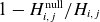 $1-H_{i,j}^{\mathrm{null}}/H_{i,j}$
with a lower bound.
$1-H_{i,j}^{\mathrm{null}}/H_{i,j}$
with a lower bound.

As a way of an example, let us consider once again $L_{{\boldsymbol{\nabla }\kern-1.2pt\boldsymbol{B}}}$
, for which the H-statistics analysis is summarised in figure 21. The plot indicates a significant cross-talk between the torsion components, giving some standing to the observation made when analysing importance. The
$L_{{\boldsymbol{\nabla }\kern-1.2pt\boldsymbol{B}}}$
, for which the H-statistics analysis is summarised in figure 21. The plot indicates a significant cross-talk between the torsion components, giving some standing to the observation made when analysing importance. The $N=5$
case does appear to show some mutual dependence between elongation features as well. One must nevertheless frame this observation in the context of the importance of these features being small and the behaviour being an outlier with respect to other
$N=5$
case does appear to show some mutual dependence between elongation features as well. One must nevertheless frame this observation in the context of the importance of these features being small and the behaviour being an outlier with respect to other $N$
.
$N$
.
Appendix C. Characterising different classes of configurations
In a dataset with a large number of elements it is daunting, or dare say impossible, to go one-by-one and check how many of those are truly distinct. This is however an important task if we are to have a thorough understanding of the database and, in particular, make sense of the optimal configuration options available. The difficulty of the task has two facets to it: what makes two configurations similar and the large number of elements (hundreds in the most benign of cases).
The most basic of notions of distance, at least formally, may be defined in input feature hyperspace. Each element in the set is uniquely defined by an input vector $\boldsymbol{x}$
of
$\boldsymbol{x}$
of $N_{\mathrm{in}}$
components, and thus, we may define
$N_{\mathrm{in}}$
components, and thus, we may define $d(i,j)=\|\boldsymbol{X}^i-\boldsymbol{X}^j\|$
as the Euclidean distance in this
$d(i,j)=\|\boldsymbol{X}^i-\boldsymbol{X}^j\|$
as the Euclidean distance in this $\mathbb{R}^{N_{\mathrm{in}}}$
space. This is however quite artificial, as some inputs refer to degrees of freedom of the magnetic axis, while others refer to the field strength more directly or the shape of cross-sections. Even though this is true, if it is the case that
$\mathbb{R}^{N_{\mathrm{in}}}$
space. This is however quite artificial, as some inputs refer to degrees of freedom of the magnetic axis, while others refer to the field strength more directly or the shape of cross-sections. Even though this is true, if it is the case that $d(i,j)\gg d(i,k)$
, we could say that
$d(i,j)\gg d(i,k)$
, we could say that $j$
is more similar to
$j$
is more similar to $i$
than
$i$
than $k$
is. To make sense of this distance though, given our mixing of different dimensions, we will at least have to normalise each dimension in some way. We adopt the extended machine learning practice of normalising these in such a way so as to have zero-averaged, unit spread populations in each dimension. This is a fair a priori, if we are to weight all components in the problem equally, assuming no fundamental difference in their domains.
$k$
is. To make sense of this distance though, given our mixing of different dimensions, we will at least have to normalise each dimension in some way. We adopt the extended machine learning practice of normalising these in such a way so as to have zero-averaged, unit spread populations in each dimension. This is a fair a priori, if we are to weight all components in the problem equally, assuming no fundamental difference in their domains.
In practice, we also find it convenient to use not the bare input feature space of size $N_{\mathrm{in}}$
, but rather its extended form including
$N_{\mathrm{in}}$
, but rather its extended form including $\tau _0$
and
$\tau _0$
and $\kappa _1$
. This extended form more fully captures the shape of the field in its real space embedding, and thus, is convenient to include. This extension of the space is not without some potential peril, in particular because these added parameters are continuous in a sense that the sampled inputs are not. This could mistakenly lead to additional linkage in space, an element to keep in mind throughout the analysis.
$\kappa _1$
. This extended form more fully captures the shape of the field in its real space embedding, and thus, is convenient to include. This extension of the space is not without some potential peril, in particular because these added parameters are continuous in a sense that the sampled inputs are not. This could mistakenly lead to additional linkage in space, an element to keep in mind throughout the analysis.
With our hyperspace set-up, and the standard Euclidean definition of distance, what constitutes a short distance? When can we deem two configurations similar and when distinct? Without a notion of a meaningful absolute distance, we must make sense of it relative to the distribution of distances with the remaining elements of the set. That way, one may determine whether two configurations are close or not. Naturally, this calls for a need to cluster the set into families of configurations sharing certain features. The entirety of the dataset can then be described through this smaller number of families, each with its own distribution. Even if the clustering was not particularly accurate, it is an important digestive tool to process the overwhelming immensity of data. The question is then, how do we cluster the data?
To cluster our set $\mathcal{S}$
of configurations into
$\mathcal{S}$
of configurations into $M$
clusters
$M$
clusters $\{\mathcal{S}_i\}$
for
$\{\mathcal{S}_i\}$
for $i=1,\ldots , M$
, we resort to the extensive literature in machine learning clustering (Kaufman & Rousseeuw Reference Kaufman and Rousseeuw2009; Wierzchoń & Kłopotek Reference Wierzchoń and Kłopotek2018). Our ultimate goal is to identify a small, finite partition of the set that distinguishes different classes of configurations, without a priori knowledge of the number of clusters that may be involved. In many clustering algorithms (K-means (Wierzchoń & Kłopotek Reference Wierzchoń and Kłopotek2018, Chapter 3.1), Gaussian mixtures (Wierzchoń & Kłopotek Reference Wierzchoń and Kłopotek2018, Chapter 3.2), BIRCH (Zhang, Ramakrishnan & Livny Reference Zhang, Ramakrishnan and Livny1996, etc.), the number of clusters is a hyperparameter that ought to be passed to the algorithm. Some more complex algorithms do not require this (e.g. spectral (Ng, Jordan & Weiss Reference Ng, Jordan and Weiss2001; Wierzchoń & Kłopotek Reference Wierzchoń and Kłopotek2018, Chapter 5) or HDBSCAN (Campello, Moulavi & Sander Reference Campello, Moulavi and Sander2013; McInnes & Healy Reference McInnes and Healy2017), but do instead offer additional complications. To decide on the number of clusters, we treat the problem as one of optimisation with respect to hyperparameters of the clustering algorithms. We define the relevant number of clusters as that corresponding to the set of clustering algorithms and hyperparameters that best clusters the set. We choose the common Calinski–Harabasz measure as a measure of goodness (Caliński & Harabasz Reference Caliński and Harabasz1974; Zhao Reference Zhao2012). This scalar measure compares the variance of elements within clusters to the variance between clusters, additionally penalising having more clusters. Such a measure is not perfect; in particular, it performs poorly for clusters that are nested or have very anisotropic shapes (what (Wierzchoń & Kłopotek Reference Wierzchoń and Kłopotek2018, Chapter 4.3) refer to as non-Voronoi clusters). We thus focus our attention upon ‘simple’ clusters. Table 5 summarises the used clustering algorithms and hyperparameters. This approach proves to be quite robust and suffice for the exploration needs in this paper.
$i=1,\ldots , M$
, we resort to the extensive literature in machine learning clustering (Kaufman & Rousseeuw Reference Kaufman and Rousseeuw2009; Wierzchoń & Kłopotek Reference Wierzchoń and Kłopotek2018). Our ultimate goal is to identify a small, finite partition of the set that distinguishes different classes of configurations, without a priori knowledge of the number of clusters that may be involved. In many clustering algorithms (K-means (Wierzchoń & Kłopotek Reference Wierzchoń and Kłopotek2018, Chapter 3.1), Gaussian mixtures (Wierzchoń & Kłopotek Reference Wierzchoń and Kłopotek2018, Chapter 3.2), BIRCH (Zhang, Ramakrishnan & Livny Reference Zhang, Ramakrishnan and Livny1996, etc.), the number of clusters is a hyperparameter that ought to be passed to the algorithm. Some more complex algorithms do not require this (e.g. spectral (Ng, Jordan & Weiss Reference Ng, Jordan and Weiss2001; Wierzchoń & Kłopotek Reference Wierzchoń and Kłopotek2018, Chapter 5) or HDBSCAN (Campello, Moulavi & Sander Reference Campello, Moulavi and Sander2013; McInnes & Healy Reference McInnes and Healy2017), but do instead offer additional complications. To decide on the number of clusters, we treat the problem as one of optimisation with respect to hyperparameters of the clustering algorithms. We define the relevant number of clusters as that corresponding to the set of clustering algorithms and hyperparameters that best clusters the set. We choose the common Calinski–Harabasz measure as a measure of goodness (Caliński & Harabasz Reference Caliński and Harabasz1974; Zhao Reference Zhao2012). This scalar measure compares the variance of elements within clusters to the variance between clusters, additionally penalising having more clusters. Such a measure is not perfect; in particular, it performs poorly for clusters that are nested or have very anisotropic shapes (what (Wierzchoń & Kłopotek Reference Wierzchoń and Kłopotek2018, Chapter 4.3) refer to as non-Voronoi clusters). We thus focus our attention upon ‘simple’ clusters. Table 5 summarises the used clustering algorithms and hyperparameters. This approach proves to be quite robust and suffice for the exploration needs in this paper.
Clustering algorithms and their hyperparameter search spaces. Clustering algorithms used (with their scikit-learn pairing; see Pedregosa et al. Reference Pedregosa2011) and the hyperparameter scan performed to choose the number of clusters in the set analysed. Only algorithms that do not treat elements as noise have been considered here.

Once a particular number of clusters and the assignment of each data point to each cluster has been achieved, we can then assess the distribution of the $N_{\mathrm{in}}$
input features within each cluster in order to deem whether such configuration families are truly different in any meaningful way or not. If so, we can then register a representative configuration from each set (see figure 6) or parametrise the family (see figure 8). This latter assessment can be made on a case-by-case basis, as the size of the set to evaluate is significantly reduced. Artificial additional clusters are not too much of a problem, so long as they only appear in reasonable numbers.
$N_{\mathrm{in}}$
input features within each cluster in order to deem whether such configuration families are truly different in any meaningful way or not. If so, we can then register a representative configuration from each set (see figure 6) or parametrise the family (see figure 8). This latter assessment can be made on a case-by-case basis, as the size of the set to evaluate is significantly reduced. Artificial additional clusters are not too much of a problem, so long as they only appear in reasonable numbers.
To illustrate the achievements of the clustering and be able to assess the results further, it is convenient to have a way of representing the set on the plane, i.e. in two dimensions. For such representation, we may use many of the existing dimensionality reduction approaches. In practice, we consider MDS (Borg & Groenen Reference Borg and Groenen2005). There are multiple approaches to dimensionality reduction under MDS,Footnote 20 attempting to faithfully preserve distances between points in different ways. No additional information is really necessary here for our purpose, given that we are using it as a simple representation vehicle, not for any quantitative end. Other dimensionality reduction techniques such as the simpler principal component analysis (Jolliffe Reference Jolliffe2011) or more sophisticated isomap (Tenenbaum, Silva & Langford Reference Tenenbaum, de Silva and Langford2000) could also be considered, but MDS is found to be most convenient in practice.
Appendix D. Detailed contributions to
$f_{\mathcal{J}}$

In this appendix we present some elements of the theoretical description of the particle precession $\omega _\alpha$
, whose near-axis form was presented in Appendix A of Rodríguez et al. (Reference Rodríguez, Helander and Goodman2024). Precession as a function of
$\omega _\alpha$
, whose near-axis form was presented in Appendix A of Rodríguez et al. (Reference Rodríguez, Helander and Goodman2024). Precession as a function of $\alpha$
(the field-line label) and
$\alpha$
(the field-line label) and $r$
(a normalised radial flux label) may be written as (Rodríguez et al. Reference Rodríguez, Helander and Goodman2024, Appendix A)
$r$
(a normalised radial flux label) may be written as (Rodríguez et al. Reference Rodríguez, Helander and Goodman2024, Appendix A)
 \begin{equation} \omega _\alpha (r,\alpha ,\lambda )= \omega _{\alpha ,-1}^{\text{non-QI}}(\lambda )\frac {\cos \alpha }{r}+\omega _{\alpha ,\mathrm{vac}}(\lambda )+\omega _{\alpha ,0}^{\text{non-QI}}(\lambda )\cos 2\alpha , \end{equation}
where $\omega _{\alpha ,-1}^{\text{non-QI}}$
and
$\omega _{\alpha ,-1}^{\text{non-QI}}$
and $\omega _{\alpha ,0}^{\text{non-QI}}$
are driven by non-omnigenous behaviour (i.e. result in
$\omega _{\alpha ,0}^{\text{non-QI}}$
are driven by non-omnigenous behaviour (i.e. result in $\alpha$
-dependent terms) (Rodríguez et al. Reference Rodríguez, Helander and Goodman2024, equations (A19) and (A21)) and the omnigenous
$\alpha$
-dependent terms) (Rodríguez et al. Reference Rodríguez, Helander and Goodman2024, equations (A19) and (A21)) and the omnigenous $\omega _{\alpha ,\mathrm{vac}}$
is a purely second-order quantity (Rodríguez et al. Reference Rodríguez, Helander and Goodman2024, equation (A15)).
$\omega _{\alpha ,\mathrm{vac}}$
is a purely second-order quantity (Rodríguez et al. Reference Rodríguez, Helander and Goodman2024, equation (A15)).
The first term in (D1), $\omega _{\alpha ,-1}^{\text{non-QI}}$
, represents the net poloidal drift due to imperfections in the first-order near-axis construction. The generally necessary departures from precise omnigeneity near
$\omega _{\alpha ,-1}^{\text{non-QI}}$
, represents the net poloidal drift due to imperfections in the first-order near-axis construction. The generally necessary departures from precise omnigeneity near $B_{\mathrm{max}}$
(Plunk et al. Reference Plunk, Landreman and Helander2019; Camacho Mata et al. Reference Camacho Mata, Plunk and Jorge2022; Rodríguez & Plunk Reference Rodríguez and Plunk2023) dominate precession sufficiently close to the magnetic axis, expecting
$B_{\mathrm{max}}$
(Plunk et al. Reference Plunk, Landreman and Helander2019; Camacho Mata et al. Reference Camacho Mata, Plunk and Jorge2022; Rodríguez & Plunk Reference Rodríguez and Plunk2023) dominate precession sufficiently close to the magnetic axis, expecting $f_{\mathcal{J}}\approx 0.5$
there due to the field-line to field-line variation. In practice, though, this contribution quickly (in
$f_{\mathcal{J}}\approx 0.5$
there due to the field-line to field-line variation. In practice, though, this contribution quickly (in $r$
) becomes overwhelmed by order
$r$
) becomes overwhelmed by order $O(r^0)$
terms, given mainly the relatively small magnitude of the magnetic drift close to
$O(r^0)$
terms, given mainly the relatively small magnitude of the magnetic drift close to $B_{\mathrm{max}}$
.
$B_{\mathrm{max}}$
.
Ignoring any QI-breaking contribution from first order, then, we may succinctly write the dominant non-omnigenous contribution to precession as (Rodríguez et al. Reference Rodríguez, Helander and Goodman2024, equation (A20))
 \begin{equation} \omega _{\alpha ,0}^{\mathrm{non-QI}} = -\frac {2mv^2}{q \bar {B}}\oint F(\lambda ,B_0)\left [B_{2c}-\frac {1}{4}\left (\frac {B_0^2d^2}{B_0'}\right )'\right ]\mathrm{d}\varphi \bigg /{\oint \frac {\mathrm{d}\varphi }{B_0\sqrt {1-\lambda B_0}}}, \end{equation}
where $\oint$
denote bounce integrals along
$\oint$
denote bounce integrals along $B_0(\varphi )$
. The integrand in square brackets (being zero) is precisely the stellarator symmetric QI condition at second order (Rodríguez & Plunk Reference Rodríguez and Plunk2023, equation (32c)). The field must therefore be sufficiently omnigenous so that
$B_0(\varphi )$
. The integrand in square brackets (being zero) is precisely the stellarator symmetric QI condition at second order (Rodríguez & Plunk Reference Rodríguez and Plunk2023, equation (32c)). The field must therefore be sufficiently omnigenous so that $\omega _{\alpha ,\mathrm{vac}}(\lambda ) \geqslant \omega _{\alpha ,0}^{\text{non-QI}}(\lambda )$
if a large fraction
$\omega _{\alpha ,\mathrm{vac}}(\lambda ) \geqslant \omega _{\alpha ,0}^{\text{non-QI}}(\lambda )$
if a large fraction $f_{\mathcal{J}}$
is to be achieved. We explicitly write
$f_{\mathcal{J}}$
is to be achieved. We explicitly write $\omega _{\alpha ,\mathrm{vac}}$
as (Rodríguez et al. Reference Rodríguez, Helander and Goodman2024, equation (A15))
$\omega _{\alpha ,\mathrm{vac}}$
as (Rodríguez et al. Reference Rodríguez, Helander and Goodman2024, equation (A15))
 \begin{equation} \omega _{\alpha ,\mathrm{vac}} = \frac {2mv^2}{q \bar {B}}\oint F(\lambda ,B_0)\left [B_{20}-\frac {1}{4}\left (\frac {B_0^2d^2}{B_0'}\right )'\right ]\mathrm{d}\varphi \bigg /\oint \frac {\mathrm{d}\varphi }{B_0\sqrt {1-\lambda B_0}}. \end{equation}
The radial gradient of the magnetic field strength dominates this term, i.e. $B_{20}$
. The larger the gradient, the more positive
$B_{20}$
. The larger the gradient, the more positive $\omega _{\alpha ,\mathrm{vac}}$
, and thus, the more maximum
$\omega _{\alpha ,\mathrm{vac}}$
, and thus, the more maximum $\mathcal{J}$
the field. This is the near-axis manifestation of the connection between MHD stability, (3.4), and maximum
$\mathcal{J}$
the field. This is the near-axis manifestation of the connection between MHD stability, (3.4), and maximum $\mathcal{J}$
.
$\mathcal{J}$
.
Appendix E. Helicity of the field
The database presented in this paper has considered so-called half-helicity QI near-axis fields only. The notion of axis helicity in stellarators was introduced by Rodríguez et al. (2022) and, for QI fields, was introduced by Camacho Mata & Plunk (Reference Camacho Mata and Plunk2023), later discussed in detail by Rodríguez et al. (Reference Rodríguez, Plunk and Jorge2025, Appendix A). These works restricted themselves to axes that can be described in cylindrical coordinates by smooth functions $R$
and
$R$
and $Z$
, so that
$Z$
, so that $\boldsymbol{r}_{\mathrm{axis}}(\phi )=R(\phi )\hat {\boldsymbol{R}}(\phi )+Z(\phi )\hat {\boldsymbol{z}}$
, where
$\boldsymbol{r}_{\mathrm{axis}}(\phi )=R(\phi )\hat {\boldsymbol{R}}(\phi )+Z(\phi )\hat {\boldsymbol{z}}$
, where $\phi$
is the cylindrical angle. Such a description is quite general and mostly sufficient, but it nevertheless excludes non-star shaped curves, knotted curves or curves with vertical segments. These exceptional cases, although rare, are not ruled out when constructing curves following Plunk & Rodríguez (Reference Plunk and Rodríguez2026), that is, by prescribing curvature and torsion directly (see figure 10). Hence, we must take additional care in defining helicity in the present context.
$\phi$
is the cylindrical angle. Such a description is quite general and mostly sufficient, but it nevertheless excludes non-star shaped curves, knotted curves or curves with vertical segments. These exceptional cases, although rare, are not ruled out when constructing curves following Plunk & Rodríguez (Reference Plunk and Rodríguez2026), that is, by prescribing curvature and torsion directly (see figure 10). Hence, we must take additional care in defining helicity in the present context.
At a high level, helicity is a count of the number of times the normal of the magnetic axis rotates around itself in a toroidal transit. This may be related to the topological notion of the self-linking number (Pohl Reference Pohl1968; Fuller Reference Fuller1971, Reference Fuller1999; Moffatt & Ricca Reference Moffatt and Ricca1992; Oberti & Ricca Reference Oberti and Ricca2016; Pfefferlé et al. Reference Pfefferlé, Gunderson, Hudson and Noakes2018; Rodríguez et al. 2022): $S_L$
is the linking number (
$S_L$
is the linking number ( $L_k$
) between our curve of interest and one generated by an infinitesimal displacement of the curve in the direction of the signed binormal vector,
$L_k$
) between our curve of interest and one generated by an infinitesimal displacement of the curve in the direction of the signed binormal vector, $\boldsymbol{r}_b^{\mathcal{\delta }}(\phi )=\boldsymbol{r}_{\mathrm{axis}}(\phi )+\delta \,\hat {\boldsymbol{\tau }}(\phi )$
, with
$\boldsymbol{r}_b^{\mathcal{\delta }}(\phi )=\boldsymbol{r}_{\mathrm{axis}}(\phi )+\delta \,\hat {\boldsymbol{\tau }}(\phi )$
, with $\delta \gt 0$
small. This is an intrinsic property of the curve and its signed frame, and thus, a ‘good’ property of the axis. In the QI scenario, for curves of odd total order, the generated
$\delta \gt 0$
small. This is an intrinsic property of the curve and its signed frame, and thus, a ‘good’ property of the axis. In the QI scenario, for curves of odd total order, the generated $\boldsymbol{r}_b^\delta$
is only closed upon two toroidal transits (Rodríguez et al. Reference Rodríguez, Plunk and Jorge2025), in which case we must divide
$\boldsymbol{r}_b^\delta$
is only closed upon two toroidal transits (Rodríguez et al. Reference Rodríguez, Plunk and Jorge2025), in which case we must divide $S_L/2$
to correct for that double transit.
$S_L/2$
to correct for that double transit.
To connect $S_L$
directly to the notion of helicity, we must invoke the Calegareanu theorem for two neighbouring curves
$S_L$
directly to the notion of helicity, we must invoke the Calegareanu theorem for two neighbouring curves $C$
and
$C$
and $C^\star$
:
$C^\star$
:
 \begin{equation} L_k(C,C^\star )=S_L(C) + \mathcal{N}. \end{equation}
Here $\mathcal{N}$
is defined as the number of rotations the unit span vector from
$\mathcal{N}$
is defined as the number of rotations the unit span vector from $C$
to
$C$
to $C^\star$
makes with respect to the signed frame of
$C^\star$
makes with respect to the signed frame of $C$
, and thus, it gives a direct connection to the counting of turns. To exploit (E1), we need some reference
$C$
, and thus, it gives a direct connection to the counting of turns. To exploit (E1), we need some reference $C^\star$
that is not aligned with the frame, as otherwise we simply recover the definition of the self-linking number (with
$C^\star$
that is not aligned with the frame, as otherwise we simply recover the definition of the self-linking number (with $\mathcal{N}=0$
).
$\mathcal{N}=0$
).
In the standard picture of helicity, the one where the curve can be defined through functions $R$
and
$R$
and $Z$
, the natural reference is what is known as the blackboard framing of the curve along the
$Z$
, the natural reference is what is known as the blackboard framing of the curve along the $z$
axis. That is, define
$z$
axis. That is, define $C^\star$
to lie outside the original curve
$C^\star$
to lie outside the original curve $C$
when looking down the
$C$
when looking down the $z$
axis, a curve that we may take as a reference
$z$
axis, a curve that we may take as a reference $\theta =0$
(see figure 22). Following (E1),
$\theta =0$
(see figure 22). Following (E1), $\mathcal{N}$
will be the number of times the signed frame crosses
$\mathcal{N}$
will be the number of times the signed frame crosses $C^\star$
(with a sign). We must also compute the linking number
$C^\star$
(with a sign). We must also compute the linking number $L_k(C,C^\star )$
, but one may prove it to vanish for the non-exceptional
$L_k(C,C^\star )$
, but one may prove it to vanish for the non-exceptional $R,Z$
-defined curves. The proof is immediate once we invoke the following proposition from Chmutov, Duzhin & Mostovoy (Reference Chmutov, Duzhin and Mostovoy2012).
$R,Z$
-defined curves. The proof is immediate once we invoke the following proposition from Chmutov, Duzhin & Mostovoy (Reference Chmutov, Duzhin and Mostovoy2012).
Lemma 1.
The self-linking number of a framed knot (the linking number between a curve $C$
and a
$C$
and a $C^\star$
generated by the framing) given by a diagram
$C^\star$
generated by the framing) given by a diagram $D$
with blackboard framing is equal to the total writhe of the diagram
$D$
with blackboard framing is equal to the total writhe of the diagram $D$
.
$D$
.
The total writhe of a knot diagram vanishes if that projection of the curve onto the plane exhibits no crossings (Chmutov et al. Reference Chmutov, Duzhin and Mostovoy2012, § 1.3.2). Additionally, by definition, our projection onto the $x-y$
plane does not have such crossings. Hence,
$x-y$
plane does not have such crossings. Hence,
 \begin{equation} \text{Helicity}=S_L, \end{equation}
as originally pointed out in Rodríguez (2022) and Rodríguez et al. (2022). When the projection has crossings, then there is a linking related correction, which we may incorporate on to the definition (as in (6.4) of Rodríguez Reference Rodríguez2022), i.e.
 \begin{equation} \text{Helicity}=S_L-L_K, \end{equation}
where $L_K$
is the Kauffmann linking number (the linking with the blackboard framing). We can generally compute this number by constructing
$L_K$
is the Kauffmann linking number (the linking with the blackboard framing). We can generally compute this number by constructing $C^\star$
deforming
$C^\star$
deforming $C$
in the direction
$C$
in the direction $\hat {\boldsymbol{z}}\times \hat {\boldsymbol{t}}$
. This works even when the axis is knotted or turning back in the toroidal angle.
$\hat {\boldsymbol{z}}\times \hat {\boldsymbol{t}}$
. This works even when the axis is knotted or turning back in the toroidal angle.
Illustrating examples of different Kauffmann number curves. Three-dimensional (top) and knot diagram (along the $z$
axis, bottom) for
$z$
axis, bottom) for $L_K=0$
and
$L_K=0$
and $L_K=1$
curves. The curve on the left has
$L_K=1$
curves. The curve on the left has $L_K=0$
as it follows from the lack of crossings. The grey curve is generated by the blackboard framing, what we take to be the reference
$L_K=0$
as it follows from the lack of crossings. The grey curve is generated by the blackboard framing, what we take to be the reference $\theta =0$
curve. The curve on the right corresponds to the tall trefoil in figure 10 and the knot diagram clearly shows a total non-vanishing writhe.
$\theta =0$
curve. The curve on the right corresponds to the tall trefoil in figure 10 and the knot diagram clearly shows a total non-vanishing writhe.

This definition of helicity, although it matches the standard definition, does however evidence that it is not fully intrinsic to the curve. It requires an external direction as well to count turns. When the curve has vertical portions, this definition will clearly break. This makes this form of helicity not a fully satisfactory property, even though it matches the qualitative description given.
Appendix F. Database statistics
In this appendix we collect the feature dependence statistical summary plots, figures 23, 24 and 25, for the various physics features discussed throughout the paper. We do so here instead of throughout the paper for clarity. We also include a table summarising the mean, maximum and minimum values of different physics features throughout the database distinguishing between different $N$
. The definitions of the features in the table can be found in the main text or in Rodriguez & Plunk (Reference Rodríguez, Plunk and Jorge2025).
$N$
. The definitions of the features in the table can be found in the main text or in Rodriguez & Plunk (Reference Rodríguez, Plunk and Jorge2025).
Feature dependence statistical summary for $A_c^{\mathrm{mhd}}$
. (a) Scatter plots showing the univariate dependence of
$A_c^{\mathrm{mhd}}$
. (a) Scatter plots showing the univariate dependence of $A_c^{\mathrm{mhd}}$
on the features
$A_c^{\mathrm{mhd}}$
on the features $\tau _{c1}$
and
$\tau _{c1}$
and $\rho _{1c}$
for the
$\rho _{1c}$
for the $N=2$
subset. (b) Summary of key statistical measures describing the dependence of
$N=2$
subset. (b) Summary of key statistical measures describing the dependence of $A_c^{\mathrm{mhd}}$
on input features. (b i) Linear correlation between the input features and
$A_c^{\mathrm{mhd}}$
on input features. (b i) Linear correlation between the input features and $A_c^{\mathrm{mhd}}$
. The different symbols indicate the Pearson and Spearman coefficients, while the colour distinguish different field periods. (b ii) Nonlinear correlation coefficient, where the colour distinguishes different field periods. (b iii) Friedman H-statistic where the size of the scatter indicates the significance of the measure compared with a null reference distribution, and the colour represents different field periods. The labels indicate which other feature they are most closely linked to. (b iv) Relative feature importance with symbols representing the PFI and cSAGE measures, and the colour representing different field periods. The values listed to the right next to the scatter indicate the coefficient of determination of a multivariate SVM model fitted to
$A_c^{\mathrm{mhd}}$
. The different symbols indicate the Pearson and Spearman coefficients, while the colour distinguish different field periods. (b ii) Nonlinear correlation coefficient, where the colour distinguishes different field periods. (b iii) Friedman H-statistic where the size of the scatter indicates the significance of the measure compared with a null reference distribution, and the colour represents different field periods. The labels indicate which other feature they are most closely linked to. (b iv) Relative feature importance with symbols representing the PFI and cSAGE measures, and the colour representing different field periods. The values listed to the right next to the scatter indicate the coefficient of determination of a multivariate SVM model fitted to $L_{{\boldsymbol{\nabla }\kern-1.2pt\boldsymbol{B}}}$
in terms of the input features.
$L_{{\boldsymbol{\nabla }\kern-1.2pt\boldsymbol{B}}}$
in terms of the input features.

Feature dependence statistical summary for $f_{\mathcal{J}}$
.
$f_{\mathcal{J}}$
.

Statistics of configuration features in the database. The table summarises the statistics of the different features of configurations (rows) for different field periods $N$
(columns). The numbers denote the average value, with the maximum and minimum values times
$N$
(columns). The numbers denote the average value, with the maximum and minimum values times ${\times}10^x$
represented as superscript and subscript respectively, where
${\times}10^x$
represented as superscript and subscript respectively, where $x$
is given by the superscript or subscript of those.
$x$
is given by the superscript or subscript of those.

Feature dependence statistical summary for $\epsilon _{\mathrm{eff}}^{\mathrm{edge}}$
.
$\epsilon _{\mathrm{eff}}^{\mathrm{edge}}$
.





















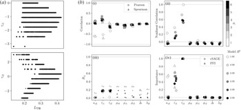


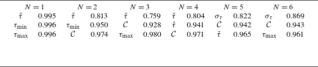


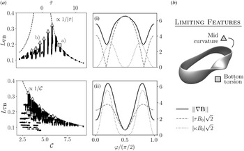


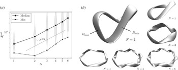


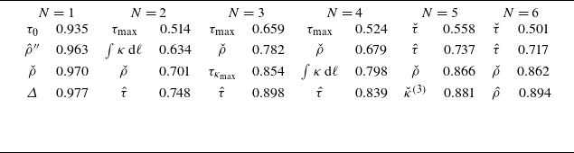


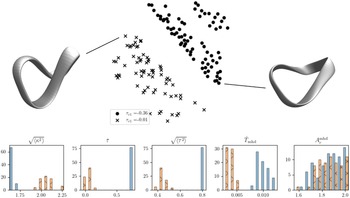


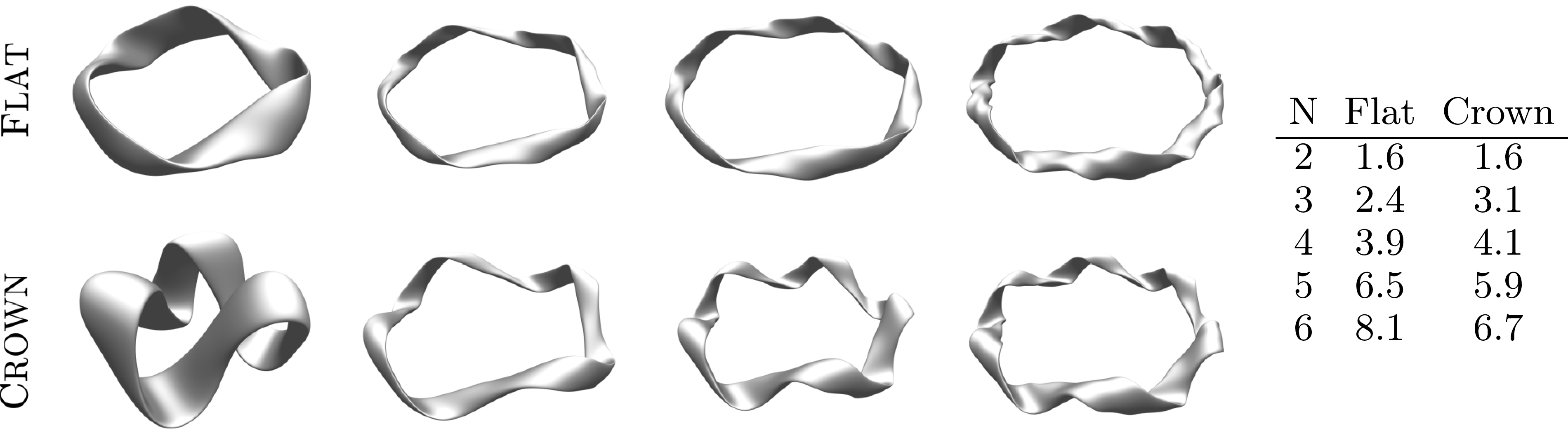





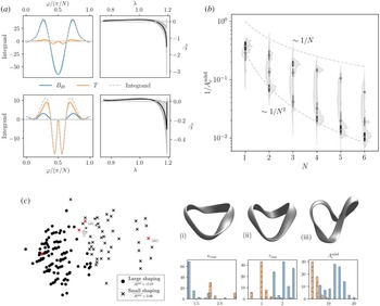


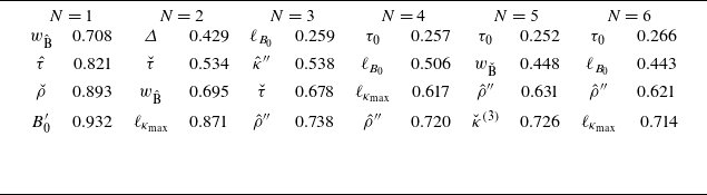


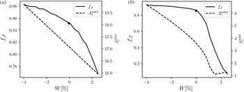


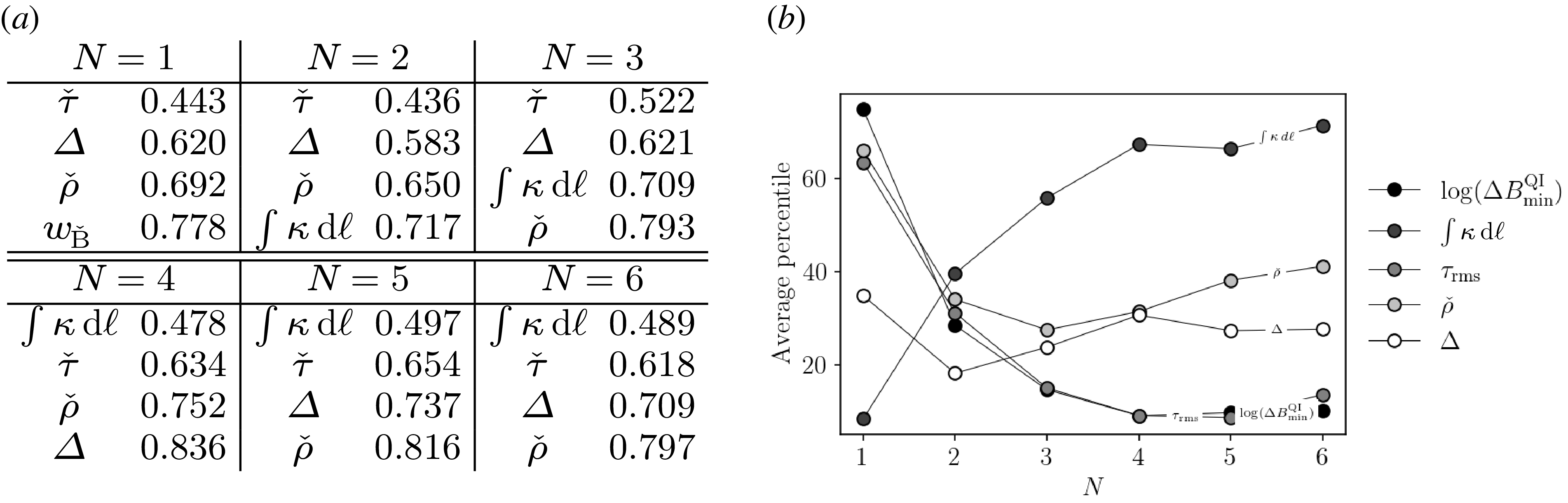


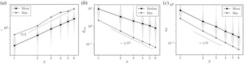


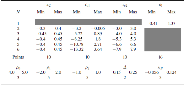


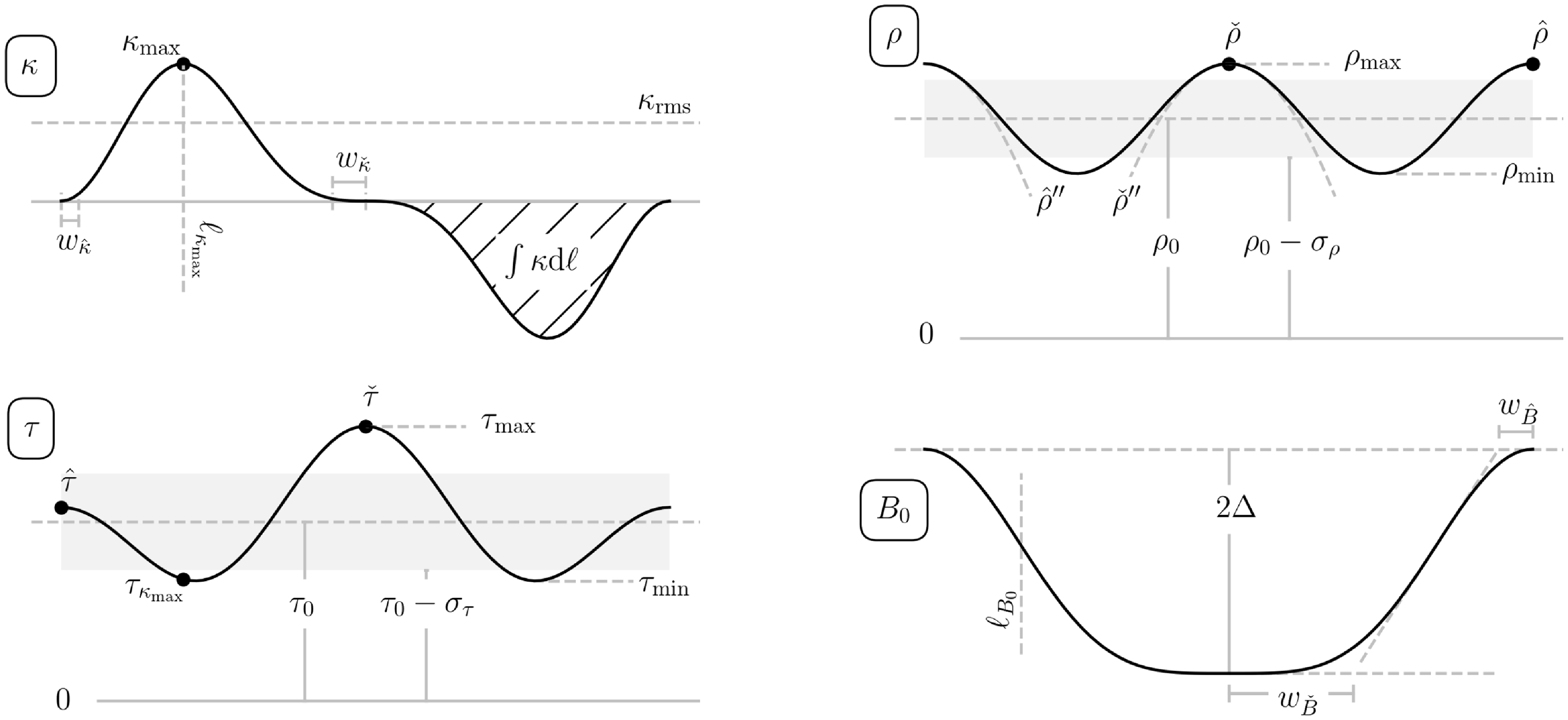
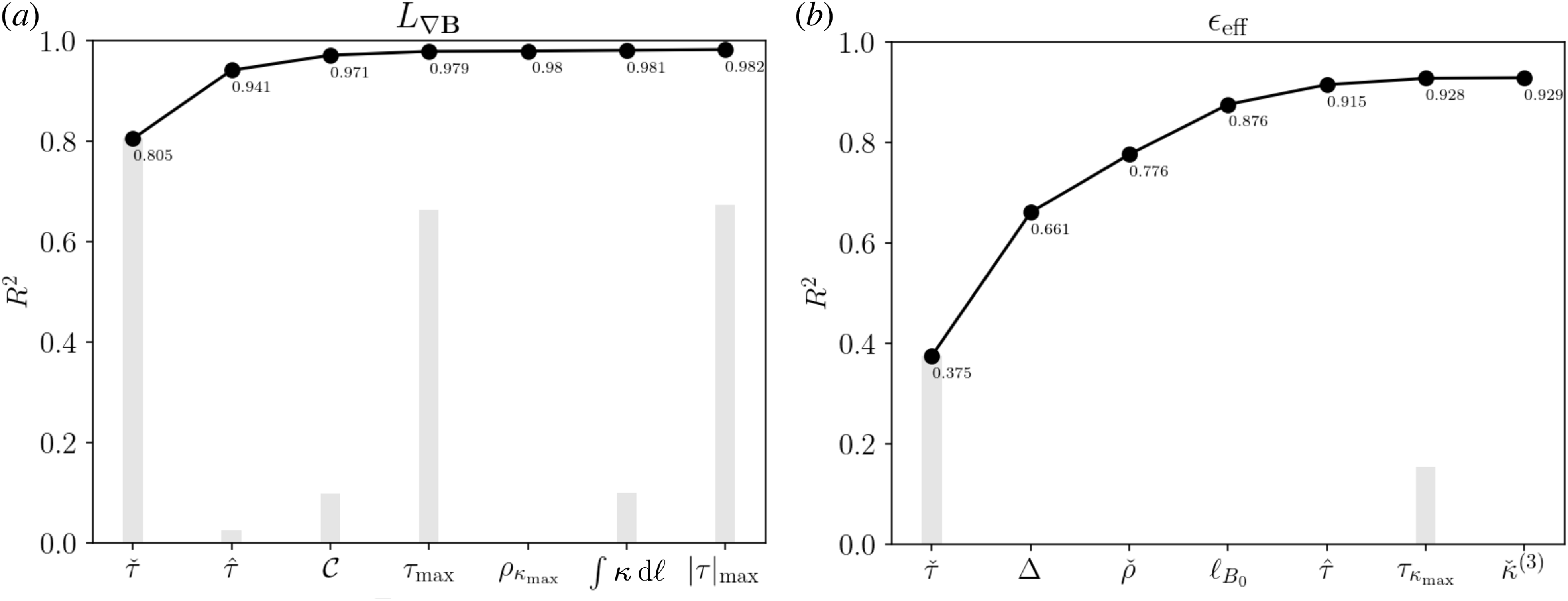


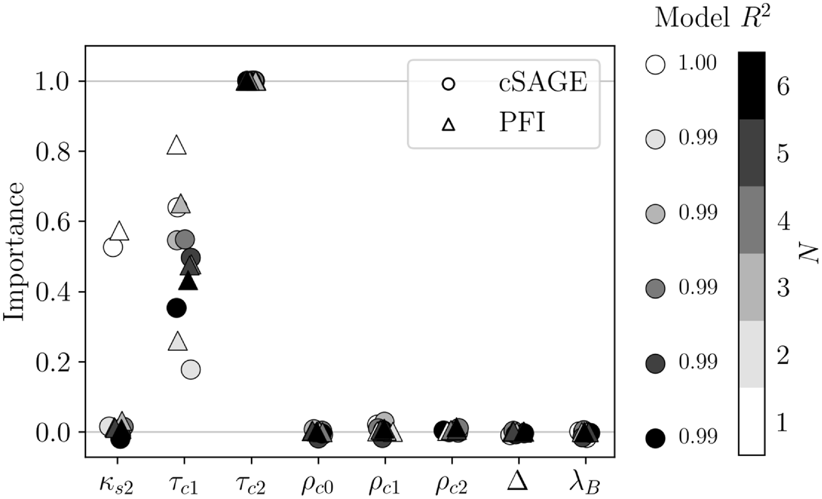


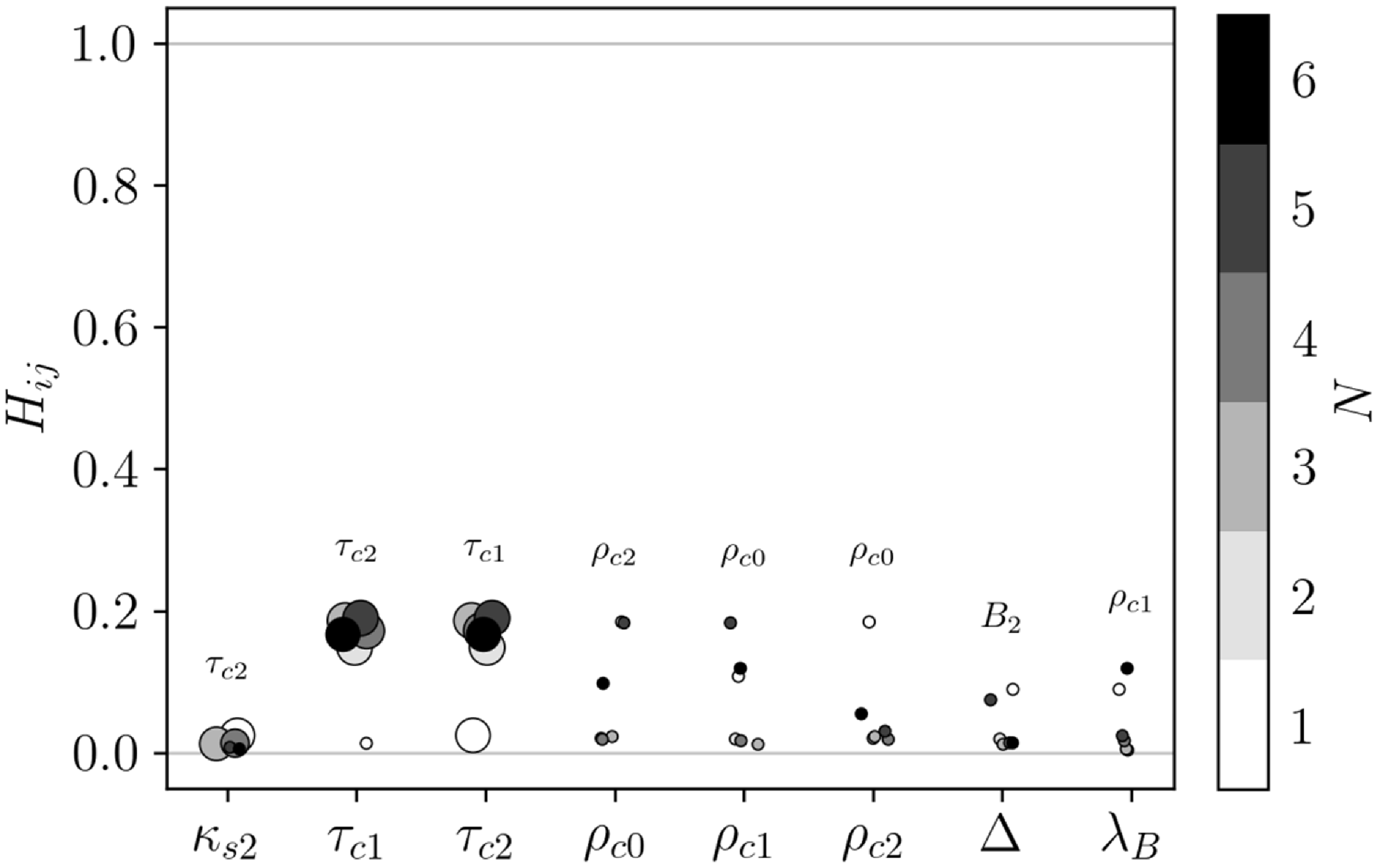


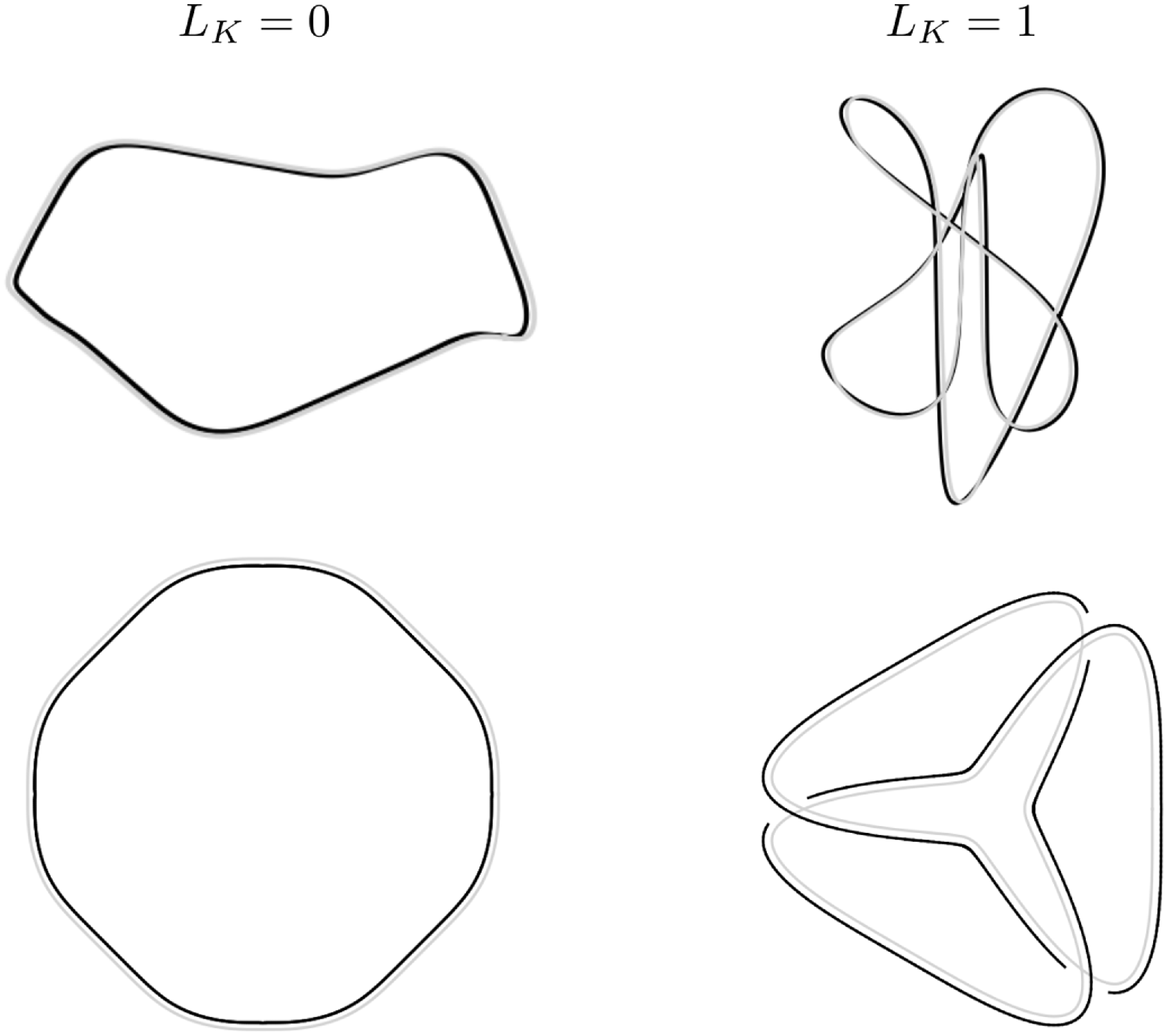


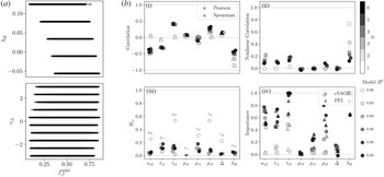

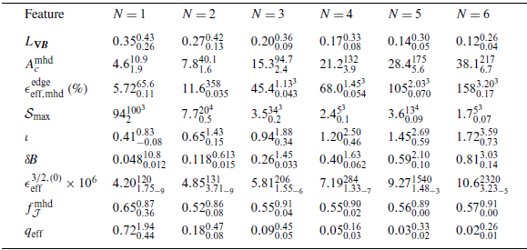


 Open access

