1.1 Degree of stability

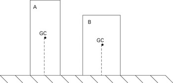
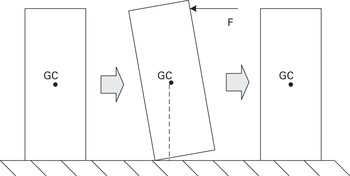
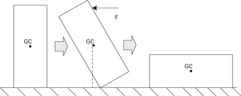
In order to illustrate the concept of stability and the “degree” of stability or “robustness” of stability, we consider two solid bodies of different size lying on the ground as shown in Figure 1.1. Their respective positions are stable. The stable position of the solid A is recovered after a small perturbation is applied to the solid, as indicated in Figure 1.2. However, if the perturbation is large enough, then the body will reach another equilibrium position, as seen in Figure 1.3, and will not return to the original (stable) equilibrium point. This system possesses multiple equilibrium states, some of which are stable but not globally stable. If one needs to determine which solid has a more “stable” equilibrium position, then it is obvious that solid B is “more stable” than solid A. More precisely, the “amount” of disturbance (i.e. perturbation) needed to push solid B away from its stable position is much larger than the amount of disturbance that is needed to push solid A away from its stable position. This “degree of stability” is related to the concept of stability region. It is clear that the stable position of solid B has a larger stability region than the stable position of solid A.

Figure 1.1

Solids A and B have the same weight and volume. The point GC indicates the center of gravity of the solid. Their positions are both stable but the stability of the position of solid B is more robust to perturbations than that of solid A. The stability region of B is larger than the stability region of A.

Figure 1.2

The solid is in a stable position. A small perturbation F is applied to the solid. After the removal of that perturbation, the solid returns to its original stable position.

Figure 1.3

The solid is in a stable position. A sufficiently large perturbation F is applied to the solid to make the solid settle down into another stable position, showing that the stable positions of this system are not globally stable.

Generally speaking, the concepts of both stability and asymptotic stability are local and do not provide information regarding how robust the system is with respect to disturbance and/or model uncertainty. The concept of stability region, on the other hand, is a global one and gives a complete picture of “the degree of stability” with respect to noise or perturbations or model uncertainty. More specifically, knowledge of the stability region provides, for a given initial condition or a specified amount of perturbation, information on whether or not the system will settle down to a desirable steady state condition.

1.2 Stability regions

We consider the following (autonomous) nonlinear dynamical system

$\dot{x}=f(x),x\in R^n.$(1.1)

It is natural to assume the function (i.e. the vector field) f: Rⁿ → Rⁿ satisfies a sufficient condition for the existence and uniqueness of the solution. The solution of (1.1) starting at $x_0$x₀ at time $t=0$t = 0 will be denoted $\varphi (t,x_0)$ϕ(t,x₀), or $x(t)$x(t) when it is clear from the context.

For an asymptotic stable equilibrium point $\widehat{x}$, there exists a number $\delta <0$δ<0 such that ||x₀ – $\widehat{x}$|| < δ implies ϕ(t, x₀) → $\widehat{x}$ as t → ∞. In other words, there exists a neighborhood of the equilibrium point such that every solution starting in this neighborhood is attracted to the equilibrium point as time tends to infinity. If δ can be chosen arbitrarily large, then every trajectory is attracted to $\widehat{x}$ and $\widehat{x}$ is called a global asymptotically stable equilibrium point. There are many physical systems containing asymptotically stable equilibrium points but not globally stable equilibrium points. A useful concept for these kinds of systems is that of the stability region (also called the region of attraction or domain of attraction). The stability region of a stable equilibrium point x_s is the set of all points x such that

$\underset{t\to \infty }{\lim }\varphi (t,x)=x_s.$(1.2)

In words, the stability region of x_s is the set of all initial conditions x whose trajectories tend to x_s as time tends to infinity. We will denote the stability region of x_s by A(x_s), and its closure by Ā(x_s), respectively; hence

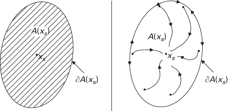
$A(x_s):=\left\{x\in R^n:\underset{t\to \infty }{\lim }\varphi (t,x)=x_s\right\}.$(1.3)

When it is clear from the context, we write A for A(x_s). From a topological point of view, the stability region A(x_s) is an open, invariant and connected set. The boundary of the stability region A(x_s) is called the stability boundary (also called the separatrix) of x_s and will be denoted by ∂A(x_s). Figure 1.4 illustrates the concept of stability region and stability boundary.

Figure 1.4

As time increases, every trajectory in the stability region A(x_s) converges to the asymptotic stable equilibrium point (SEP) x_s and every trajectory on the stability boundary evolves on the stability boundary.

The concept of stability region of an asymptotic stable equilibrium point can be extended to that of other types of attractors. For example, the stability region of an asymptotic stable closed orbit, γ, is defined as follows:

$A(\gamma )=\left\{x\in R^n:\underset{t\to \infty }{\lim }d(\varphi (t,x),\gamma )=0\right\}$

where d(.,.) is a distance function. The stability regions of other types of attractors, such as asymptotically stable quasi-periodic solutions and asymptotically stable chaotic trajectories, are similarly defined. Global stability (i.e. stability in the large) rarely occurs in physical and engineering systems due to physical and operational limits, such as saturations and control actions. In addition, the cost of designing systems to be globally stable, when feasible, is usually very high. These factors make the task of determining stability regions of nonlinear systems of great importance for practical application. It is fair to state that knowledge of the stability region of an attractor is equally important to verification of the stability of the attractor itself.

Knowledge of the stability region is essential in a variety of application areas such as direct methods for power system transient stability analysis [Reference Chiang, Chu and Cauley51,Reference Chiang, Wu and Varaya65,Reference Davy and Hiskens81,Reference Hill and Mareels121,Reference Praprost and Loparo207,Reference Sauer and Pai224,Reference Varaiya, Wu and Chen257,Reference Venkatasubramanian, Schattler and Zaborsky264,Reference Xin, Gan, Qiu and Qu280], stabilization of nonlinear systems [Reference da Silva and Tarbouriech101,Reference Henrion, Tarbouriech and Garcia120,Reference Kokotovic and Marino147,Reference Meza, Santibanez and Campa179,Reference Milani183,Reference Shim and Seo227,Reference Tibken250,Reference Toussaint and Basar253,Reference Xin, Gan, Huang and Wang279], decentralized control design for nonlinear systems, power system voltage collapse problems [Reference Hill and Mareels121,Reference Hiskens and Hill126], schemes for choosing manipulator specifications and parameters in robotics [Reference Bondi, Casalino and Gambardella26,Reference Ortega, Loria and Kelly196], the design of associative memory in artificial neural networks [Reference Ciliz and Harova71,Reference Djukanovic, Sobajic and Pao83,Reference Hopfield127], solution methods for nonlinear optimization problems [Reference Chiang, Chen, Reddy, Pardalos and Coleman48,Reference Chiang and Chu49,Reference Chiang, Lee, Lee and El-Sharkawi56,Reference Chiang, Wang and Jiang62,Reference Lee and Chiang162,Reference Lee and Chiang163], the effect of discretized feedback in a closed loop system on stability [Reference Laila, Lovera and Astolfi155], and so forth. Knowledge of the stability region of a stable limit cycle is critical in areas such as biology [Reference Baer, Li and Smith19] and robotics [Reference Westervelt, Grizzle and de Wit274,Reference Westervelt, Grizzle and Koditschek275].

Determining stability regions of nonlinear dynamical systems is an old problem, and yet it remains challenging. Recent advances in theoretical developments of stability regions and in the development of effective methods for estimating stability regions offer promising results to meet the challenges. These advances can be classified as follows.

Theoretical development:

• characterization of a subset of stability regions of general nonlinear dynamical systems,

• complete characterization of stability boundaries of equilibrium points and attractors of a fairly large class of nonlinear dynamical systems,

• complete characterization of stability boundaries of fixed points of a class of time-discrete nonlinear dynamical systems,

• characterization of stability boundaries of two-time-scale systems,

• complete characterization of stability boundaries of a class of nonlinear non-hyperbolic dynamical systems,

• characterization of relevant stability boundaries of a class of nonlinear dynamical systems.

Methods for estimating the stability region:

• optimal estimation of stability regions of a fairly large class of continuous nonlinear dynamical systems,

• optimal estimation of stability regions of second-order systems,

• optimal estimation of stability regions of a large class of discrete dynamical systems,

• constructive approach to iteratively improve estimations of stability regions,

• optimal estimation of relevant stability regions of a class of nonlinear dynamical systems.

In this book, a comprehensive treatment of these contributions is presented in a structured way, followed by advanced topics on stability regions and by illustrations of stability-region-based practical applications.

1.3 Characterization and estimation of stability regions

It is not easy to trace the first attempt to address the issue of stability regions in the literature, but the history of development of the concept of stability sheds some light on it. The subject of stability has attracted a significant, if not the most, amount of research and development in the area of nonlinear system analysis, design and control. The theory of stability and, in particular, methods to estimate stability regions are related to energy function theory. The mathematicians Leonhard Paul Euler and Joseph-Louis Lagrange, in the eighteenth century, established relations between the equilibrium point and stability with maxima and minima of energy functions. Aleksandr Mikhailovich Lyapunov (1857–1918), inspired by his master’s thesis on fluid dynamics, developed a general theory of stability in his PhD thesis: The general problem of the stability of motion (1892). Lyapunov derived sufficient conditions for stability based on the existence of a scalar function, nowadays called the Lyapunov function in his honor. George David Birkhoff (1884–1944) made an important contribution by developing stability theory for the asymptotic behavior of trajectories of differential equations.

Krasovskii was probably the first to prove an invariance principle [Reference Krasovskii149]. This principle explores the concept of limit sets introduced by Birkhoff. Joseph P. LaSalle, who received his PhD in 1941, developed a similar invariance principle in 1960 [Reference LaSalle158]. LaSalle’s invariance principle is probably the first tool proposed for estimating stability regions in a systematic way. The work of Krasovskii and LaSalle led to the development of the expression of stability region estimates in the form of level sets of Lyapunov-like functions.This pioneering work has sparked the development of a great number of methods for estimating stability regions of high-dimensional nonlinear systems.

The existing methods for estimating stability regions proposed in the literature can be classified into Lyapunov-function-based methods and non-Lyapunov-function-based methods. Unfortunately, the vast majority of methods always offer rather conservative estimations of stability regions; in other words, these methods offer estimated stability regions which are only a (small) subset of entire stability regions. This conservative estimation can lead to serious consequences. For example, conservative estimates of the stability region may result in unnecessary interruptions in the operation of power systems and in expensive over-design of control systems. Thus, there is a serious need for the development of effective methods for accurately estimating stability regions of high-dimensional nonlinear dynamical systems.

Lyapunov-function-based methods have been popular for estimating the stability regions of stable equilibrium points. This class of methods is applicable to large-scale nonlinear systems but may suffer from overly conservative estimation of stability regions. The degree of conservativeness of Lyapunov-function-based methods in estimating stability regions depends on the underlying Lyapunov function and the associated value of the critical level. Finding a good Lyapunov function for estimating stability regions is not an easy task. There is no systematic way to derive a Lyapunov function for general nonlinear dynamical systems. Recent advances along this line of research and development include the proposal of maximal Lyapunov functions [Reference Vannelli and Vidyasagar256], the optimal estimation of stability regions based on a given Lyapunov function [Reference Chiang and Fekih-Ahmed53], LMI optimization techniques for constructing Lyapunov functions, and estimating stability regions for polynomial dynamical systems [Reference Chesi, Garulli, Tesi and Vicino41,Reference Coutinho, Bazanella, Trofino and Silva76,Reference Johansen137,Reference Levin164,Reference Tan and Packard247,Reference Tibken250,Reference Topcu, Packard, Seiler and Wheeler252] and for non-polynomial systems [Reference Chesi39]. These optimization-based methods entail high computation effort, tending to grow rapidly with the system dimension, making them unsuitable for estimating stability regions of high-dimensional nonlinear dynamical systems. The LMI-based estimation methods generally yield (overly) conservative estimations of stability regions.

Another advance is the constructive Lyapunov function methodology for determining optimal Lyapunov functions to estimate stability regions [Reference Chiang and Thorp60]. The constructive methodology yields a sequence of estimated stability regions which form a strictly monotonic increasing sequence, and yet each of them is contained in the stability region of the system under study. The constructive methodology can either stand by itself or be used with existing methods serving as the input to the constructive methodology. This methodology can reduce the conservativeness in estimating stability regions via the Lyapunov function approach.

There are very few methods which are able to estimate the entire stability region. They all entail serious computational problems, making their application impractical. For example, Zubov’s method [Reference Grune and Wirth106,Reference Margolis and Vogt175] offers a technique for computing the entire stability region via the “optimal” Lyapunov function. However, constructing this “optimal” Lyapunov function requires solving a set of nonlinear partial differential equations (PDEs) which are difficult, if not impossible, to solve. Because of this problem, several techniques have been proposed which attempt to approximate the solution of the PDEs, but with limited success. Furthermore, it has been found that even for some second-order systems the use of approximated solutions to construct the “optimal” Lyapunov function still results in rather conservative estimations.

Another method which attempts to reduce the conservativeness in estimating the stability boundary was proposed in [Reference Genesio, Tartaglia and Vicino97], in which the estimated stability boundary was synthesized from a number of system trajectories obtained by backward integration. This method, known as the trajectory reversing method [Reference Genesio, Tartaglia and Vicino97,Reference Genesio and Vicino99,Reference Loccufier and Noldus168], is suitable only for low-dimensional systems due to its excessive computational burden. Other methods for estimating the stability region include approximating the stability boundary by polytopes [Reference Psiaki and Luh208] and the cell-to-cell mapping method [Reference Hsu128].

A majority of the existing proposed methods for estimating stability regions are only applicable to low-dimensional nonlinear systems. Very few of them are applicable to high-dimensional nonlinear systems (say several hundred or thousands of dimensions). To be practical, estimation methods need to be able to deal with very large-scale systems (say, tens of thousands of state variables).

An important breakthrough in the development of the theory of stability regions occurred in the 1980s with the formulation of a comprehensive theory of stability regions and a complete characterization of the stability regions of a class of nonlinear dynamical systems [Reference Chiang, Hirsch and Wu54]. This class of nonlinear dynamical systems is characterized by its ω-limit set being composed of equilibrium points and limit cycles. A conceptual method based on the complete characterization derived in [Reference Chiang, Hirsch and Wu54], when feasible, can find the entire stability region. This method is based on a complete characterization of the stability boundary via the stable manifolds of unstable equilibrium points and unstable limit cycles on the stability boundary. For low-dimensional nonlinear dynamical systems, the derivation of the stable manifolds can be achieved by numerical methods. However, current computational methods are inadequate for computing the stable manifolds of unstable equilibrium points and/or of unstable limit cycles of high-dimensional nonlinear dynamical systems.

Knowledge of the complete characterization of a stability boundary has led to the development of several effective methods for accurate estimation of stability regions. By exploring the complete characterization of the stability boundary, several computational schemes for optimally estimating the stability regions have been developed, see for example [Reference Chiang and Fekih-Ahmed53]. These complete characterizations have also led to the development of effective methods to estimate relevant parts of the stability boundary. These methods have been fundamental to advancing a variety of important practical applications.

1.4 Practical applications of stability regions

Estimating or determining stability regions is central to solving many problems arising in sciences and engineering. The following list is a non-exhaustive enumeration of applications where knowledge of stability regions plays an important role.

1. 1. Biology:

   • micromolecules and macromolecules;

   • dynamics of ecosystems.

2. 2. Biomedicine:

   • dynamics of the immune response;

   • human respiratory models.

3. 3. Control:

   • sliding control systems;

   • control of nonlinear systems;

   • linear systems with saturated controls;

   • control of polynomial systems.

4. 4. Economics:

   • economic growth rate;

   • carrying capacity of the human population.

5. 5. Robotics:

   • asymptotically stable walking cycle of a bipedal robot;

   • regulator design of robot manipulators.

6. 6. Power grids and power systems:

   • direct power system transient stability analysis;

   • dynamic voltage stability analysis.

7. 7. Power electronic circuits:

   • power-electronic-based converters;

   • DC-to-DC converters.

8. 8. Neural networks:

   • dynamic recurrent neural networks;

   • associative memory;

   • Hopfield neural network models.

9. 9. Optimization problems:

   • unconstrained optimization problems;

   • constrained optimization problems.

We briefly describe some of the above applications based on knowledge of stability regions.

1.4.1 Immune response

Stability regions provide insight into the analysis of the immune response where interaction among lymphocyte populations, antigens and antibiotics occurs [Reference Gunther and Hoffman110,Reference Kaufman and Thomas139,Reference Segel225,Reference Villafuerte and Mondié267]. The coexistence of multiple equilibriums has been reported in these models and the outcome of a treatment depends not only on how antigens are administered but also on the initial condition of the system when the treatment began. Depending on the initial condition, the dynamics of the treatment will converge to the attractor whose stability region contains the initial condition.

The immune system is primarily composed of a large number of cells called lymphocytes. Lymphocytes produce antibodies that bind to invading organisms (antigens) in order to eliminate them. An animal can produce a very large number of different antibodies (10⁶ to 10⁷) [Reference Gunther and Hoffman110]. The presence of an antigen stimulates the proliferation of cells (lymphocytes) with the specific antibody for that invader. The following set of differential equations models the dynamics of positive and negative cells of the immune system:

$\begin{array}{l}{\dot{x}}_{+}=x_{+}[R(x_{-},x_{+})-D(x_{-},x_{+})-k_4]+k_5\\ {\dot{x}}_{-}=x_{-}[R(x_{+},x_{-})-D(x_{+},x_{-})-k_4]+k_5\end{array}$

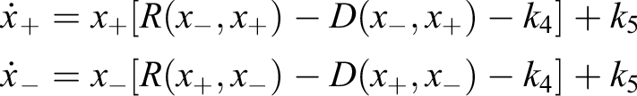
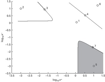
where x₊ and x₋ respectively represent the concentrations of positive and negative cells in the organism. The constant k₅ is an influx rate term while k₄ is a death rate term. The function R is a replication rate that describes the proliferation of the positive cells, while the function D is a death rate due to killing by antibodies or anti-antibodies. A typical phase portrait of the immune dynamical system is shown in Figure 1.5. Typically, immunization systems have four asymptotically stable equilibrium points: the virgin state, indicated as equilibrium #1 in Figure 1.5, where the concentrations of both positive and negative cells are low, the immune state, depicted as equilibrium #5, where the concentration of positive cells is much larger than that of negative cells, the anti-immune state, equilibrium #2, where the concentration of negative cells is high compared to the concentration of positive cells, and a suppressed state, equilibrium #6, where both concentrations are high. The immunization problem consists of designing a proper perturbation to the immune system, an immunization shot for example, such that the initial condition of the system after perturbation lies inside the stability region of the immune state equilibrium point, highlighted in gray in Figure 1.5. As a result, the immune system of the organism will abandon the virgin state equilibrium #1 and settle down in the immune state equilibrium #5.

Figure 1.5

The stability region of the immune state (equilibrium #5) of a typical immunization system is highlighted. The immune system contains four asymptotically stable equilibrium points (SEPs): equilibriums #1 (virgin state), #2 (anti-immune state), #5 (immune state) and #6 (suppressed state). Their stability boundaries are depicted in this figure as black lines. Equilibriums #3, #4 and #7 are unstable equilibrium points lying on the stability boundaries of these four SEPs.

1.4.5 Nonlinear control systems

Characterization of the stability region is of great importance in modern nonlinear control systems [Reference da Silva and Tarbouriech101,Reference Henrion, Tarbouriech and Garcia120,Reference Kokotovic and Marino147,Reference Meza, Santibanez and Campa179,Reference Milani183,Reference Shim and Seo227,Reference Tibken250,Reference Toussaint and Basar253]. It has been recognized that high feedback control gain can destabilize closed loop nonlinear systems [Reference Kokotovic and Marino147,Reference Toussaint and Basar253]. Contraction of the stability region due to high feedback gain contributes to this destabilization. The task of maximizing the size of the stability region has become a design objective in nonlinear system analysis and controller design [Reference Wada270,Reference Shyu and Chen230], including the design of linear system controllers with saturation [Reference Coutinho and da Silva77,Reference da Silva and Tarbouriech101,Reference Henrion, Tarbouriech and Garcia120,Reference Milani183].

The characterization of stability regions of nonlinear control systems is important in practical applications, see for example [Reference Ailon, Segev and Arogeti3,Reference Chiang, Stefanopoulou and Jankoviv43,Reference Dong, Cheng and Oin84,Reference Jadbabaie and Hauser133,Reference Langson and Allevne154,Reference Zhong287]. Local stability analysis is based on a linearized model and does not provide information regarding the nature of the stability region. The stability region can only be characterized by taking into account the nonlinearity of the underlying nonlinear system. We present one example of controller design: one where the stability region shrinks with the increase in controller gain. This example serves to illustrate that overlooking both the nonlinear terms and the stability region characterization in the controller design can result in a closed loop nonlinear system with a very small size stability region and, consequently, with a small degree of robustness with respect to both state and parameter perturbations.

Consider the following nonlinear system from [Reference Kokotovic and Marino147]:

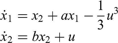$\begin{array}{l}{\dot{x}}_1=x_2+a{x}_1-\frac{1}{3}{u}^3\\ {\dot{x}}_2=b{x}_2+u\end{array}$(1.4)

where u ∈ R is an input, a and b are unknown parameters satisfying |a| < c and |b| < c, with c > 0 as an upper bound for the uncertain parameters a and b. The objective is to design a state feedback controller that stabilizes the origin of this system. For this purpose, consider the linearization of system (1.4)

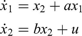$\begin{array}{l}{\dot{x}}_1=x_2+a{x}_1\\ {\dot{x}}_2=b{x}_2+u\end{array}$(1.5)

with the following feedback control:

$u=-{\gamma }^2{x}_1-y{x}_2.$

u = − γ²x₁ − yx₂.

(1.6)

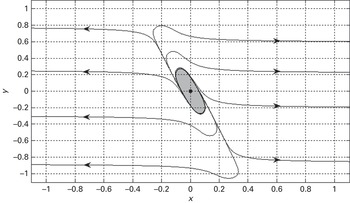
By substituting (1.6) into (1.5) and computing the eigenvalues of the closed loop system, we conclude that the equilibrium point (0.0, 0.0) (i.e. the origin) of the linearized closed loop system is asymptotically stable, for any |a| < c and |b| < c, if γ >2c. Assuming the same state feedback (1.6) is employed to stabilize the nonlinear system (1.4), Figure 1.6 shows the stability region of the origin of the nonlinear closed loop system for a=0, b=0, c=1 and γ = 4. Since the eigenvalues of the Jacobian matrix evaluated at the origin are $-2\mp j2\sqrt{3}$, the origin of the closed loop system is indeed asymptotically stable. In spite of that, it is clear from Figure 1.6 that the stability region is too small to ensure robustness with respect to perturbations.

Figure 1.6

Illustration of the stability region of the nonlinear closed loop system (1.4) and (1.6) for a = b = 0, c = 1 and γ = 4 and some system trajectories which serve to verify the position of the stability boundary.

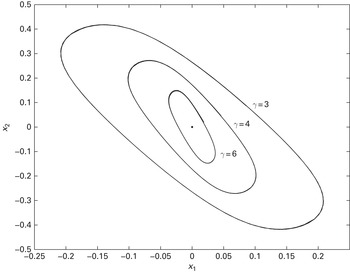
There is a nonlinear relationship between the stability boundary and the controller. Numerical studies show that the stability boundary of (0.0, 0.0) (the origin) is composed of an unstable limit cycle. In addition, the stability region shrinks as the controller gain γ increases, shown in Figure 1.7. This simple example illustrates that the linearization approach for controller design is completely independent of the size of the stability region. A design for a good-performance controller based on the linearized model can lead to very small size stability regions. As a consequence, it is important to adopt the size of the stability region as one criterion in designing linear controllers for controlling nonlinear systems.

Figure 1.7

The stability region of the origin of the nonlinear closed loop system (1.4) and (1.6) shrinks as the controller gain γ increases. As the feedback gain increases from a magnitude of 3 to 6, the corresponding stability boundary significantly shrinks.

1.5 Purpose of this book

The main purpose of this book is to present a comprehensive framework for developing the theory of stability regions of different types of nonlinear dynamical systems. Advanced topics on stability regions will also be presented. In addition, this book presents a unified framework to estimate stability regions of nonlinear dynamical systems. Optimal schemes for estimating stability regions of nonlinear dynamical systems will be presented for different types of these systems. Practical applications of stability regions to several topics of engineering are demonstrated. The transformation of nonlinear optimization problems into the stability region problem is also presented and shown to be a fruitful research and development area.

Nonlinear dynamical systems arising from different engineering disciplines and the sciences are vast and appear in a variety of different forms. This book covers the following types of nonlinear analysis:

• continuous nonlinear dynamical systems,

• discrete-time nonlinear dynamical systems,

• complex continuous nonlinear dynamical systems,

• constrained continuous nonlinear dynamical systems,

• two-time-scale nonlinear dynamical systems,

• interconnected nonlinear dynamical systems,

• non-hyperbolic nonlinear dynamical systems.

From computational viewpoints, effective schemes for estimating the stability regions of the above different types of nonlinear dynamical systems are described and analyzed. In addition, a constructive methodology for optimally estimating stability regions will be presented and analyzed.

From a practical viewpoint, knowledge of stability regions has significant applications. This book describes practical applications of stability regions to the following areas:

• direct stability analysis in electric power systems,

• stability-region-based nonlinear optimization methods.

We believe that solving challenging practical problems efficiently can be accomplished through a thorough understanding of the underlying theory, in conjunction with exploring the special features of the practical problem under study to develop effective solution methodologies. This book covers both comprehensive theoretical developments of stability regions and comprehensive solution methodologies for estimating stability regions.

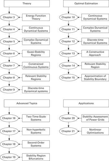
There are 22 chapters contained in this book. These chapters can be classified as shown in Figure 1.8.

Figure 1.8

An overview of the organization and content of this book.

In summary, this book presents theoretical developments of stability regions of various types of nonlinear dynamical systems as well as solution methodologies for estimating these stability regions. The interplay between stability regions and bifurcations is also described. On the application side of the knowledge of stability regions, the long-standing research and development of fast stability-region-based methods for power system transient stability analysis and the emerging area of stability-region-based nonlinear optimization methods are presented in detail. In particular, this book

• develops a comprehensive theory of stability regions of nonlinear dynamical systems (including continuous and discrete systems),

• presents a complete characterization of stability boundaries of a class of nonlinear dynamical systems,

• presents a complete characterization of stability boundaries of a class of complex nonlinear dynamical systems,

• develops a comprehensive theory of stability regions of two-time-scale nonlinear dynamical systems,

• develops a comprehensive theory of stability regions of a class of non-hyperbolic nonlinear dynamical systems,

• develops schemes for estimating stability regions of general nonlinear dynamical systems,

• presents optimal schemes for estimating stability regions of a class of nonlinear dynamical systems,

• presents a complete characterization of relevant stability regions of a class of nonlinear dynamical systems,

• presents optimal schemes for estimating relevant stability regions of a class of nonlinear dynamical systems.

It is expected that the reader has some familiarity with the theory of ordinary differential equations and nonlinear dynamical systems. This book can be read sequentially, chapter to chapter, or the reader may jump to chapters of interest. The minimum suggested path would be Chapters 1, 2, 3, 4, 6, 8, 10, 13, 18 and 22. This sequence will give to the reader a very comprehensive understanding of the theory of stability regions for continuous dynamical systems and the methods for estimating stability regions. Readers may want to include Chapters 5 and 11 to gain some insight into the characterization of the stability boundaries of a more general class of continuous dynamical systems, i.e. systems that exhibit complex behavior such as closed orbits and chaos.

Chapters 9 and 12 present a complete characterization of stability boundaries and methods to estimate the stability region of nonlinear discrete-time systems. They can be read separately but the contents of Chapters 4 and 10 would be useful background. Chapter 7 extends the characterization of stability boundaries developed in Chapter 4 to the class of nonlinear constrained systems, i.e. systems that are modeled by a set of differential and algebraic equations. It is suggested that Chapter 4 should be read before Chapter 7. The advanced topic chapters require some working knowledge of the theory chapters and of the optimal estimation chapters. The same is true for the application chapters.