2. Numerical model and model set-up

The governing equations used herein are the incompressible Euler equations with the Boussinesq approximation. A rigid lid is employed and rotational affects are not considered. The stable background densities considered here have the form of two thin pycnoclines separating three layers of constant densities $\rho _3$ in the lower layer, $\rho _2$ in the middle layer and $\rho _1$ in the upper layer with $\rho _3 > \rho _2 > \rho _1$. In dimensional terms the stratifications have the form

(2.1)\begin{align} \bar{\rho}(z) = \rho_3 - \frac{1}{2}\left(\rho_3-\rho_2\right) \left(1 +\tanh\left(\frac{z-z_2}{d_2}\right)\right) - \frac{1}{2}\left(\rho_2-\rho_1\right) \left(1 +\tanh\left( \frac{z-z_1}{d_1}\right)\right), \end{align}

where $z_2< z_1$ are the centres of the two pycnoclines and the constants $d_1$ and $d_2$ determine their thicknesses. The density is non-dimensionalized and scaled via

(2.2)\begin{equation} \rho = \rho_0\left(1 + \Delta\rho\tilde{\rho}\right), \end{equation}

where $\rho _0 = {1}/{2}(\rho _1 + \rho _3)$ is the reference density used in the Boussinesq approximation and $\rho _0\Delta \rho = \rho _3-\rho _1$. The dimensionless density $\tilde {\rho }$ is then approximately equal to $-0.5$ and 0.5 at the top and bottom of the water column respectively if the pycnoclines are thin compared with their distance from the upper and lower boundaries as assumed here. The remaining terms in the governing equations are non-dimensionalized using the constant water depth $H$ as the length scale, $T = \sqrt {H/(g\Delta \rho )}$ as the time scale and $U = H/T$ as the velocity scale. This gives the dimensionless equations (dropping the tilde on the dimensionless density)

(2.3a)$$\begin{gather} u_t+uu_x+wu_z=- p_x, \end{gather}$$

(2.3b)$$\begin{gather}w_t+uw_x+ww_z=- p_z-\rho, \end{gather}$$

(2.3c)$$\begin{gather}\rho_t+u\rho_x+w\rho_z=0, \end{gather}$$

(2.3d)$$\begin{gather}\boldsymbol{\nabla} \boldsymbol{\cdot} \boldsymbol{u}=0 \end{gather}$$

as the governing equations, where $z\in [-1,0]$ is now dimensionless. Here $\boldsymbol {u} = (u,w)$ is the velocity in the vertical $xz$ plane and $p$ is a dimensionless dynamic pressure. The total dimensional pressure is

(2.4)\begin{equation} p^* = \left(\rho_0 \Delta\rho gH\right) p - \rho_0gHz \end{equation}

up to an arbitrary constant. For simulations of interacting ISWs these equations are solved using a two-dimensional non-hydrostatic internal gravity wave model (Lamb Reference Lamb1994, Reference Lamb2007). The model uses Godunov flux limiting which acts as an implicit large-eddy simulation model and a variable time step satisfying a Courant–Friedrichs–Lewy condition. The dimensionless background stratifications are given by

(2.5)\begin{equation} \bar{\rho}(z) =-\frac{1}{2}\Delta\rho_1\tanh\frac{z-z_1}{d_1} - \frac{1}{2}(1-\Delta\rho_1)\tanh\frac{z-z_2}{d_2}, \end{equation}

with $-1 < z_2 < z_1 <0$ so the upper pycnocline is centred at $z_1$ and the lower pycnocline is centred at $z_2$. The upper-, middle- and lower-layer thickness are taken as $h_1 = -z_1$, $h_2 = z_1-z_2$ and $h_3 = 1+z_2$. We only consider thicknesses $d_1=d_2=0.04$. For stratifications with pycnoclines close to the top or bottom boundaries the bottom to surface density difference may be slightly less than 1. Figure 1 shows some sample stratifications. The simulations are initialized with ISW solutions of the DJL equation (see next section) which are interpolated onto the computational grid.

Figure 1.

Sample stratifications of (a) $\bar \rho$ and (b) $N^2$ for $(z_1,z_2) = (-0.25, -0.9)$ and $d_1=d_2=0.04$ for $\Delta \rho _1 = 0.55$ (solid) and $0.6$ (dashed).

3. Theoretical background

In this section some relevant theoretical results are briefly presented. We first discuss the Gardner equation which is an approximate model for weakly nonlinear long waves. This equation is often used to model ISWs in a stratified fluid; however, the results presented below show that it is not useful for the interaction of waves of opposite polarity. Following this is a discussion of the DJL equation which gives exact solitary wave solutions of the governing equations (2.3) which are used to initialize the simulations. The DJL solutions show that solitary wave amplitudes are limited and that as the limiting amplitude is approached the waves grow indefinitely in length. The resulting conjugate flow in the horizontally uniform centre of long waves is discussed in the final subsection. The conjugate flow determines limiting wave amplitudes and is used to determine when ISW solutions of the governing equations exist. The procedure for doing so is described in the following section.

3.1. Weakly nonlinear theory

The Gardner equation (Grimshaw, Pelinovsky & Talipova Reference Grimshaw, Pelinovsky and Talipova1997; Talipova et al. Reference Talipova, Pelinovsky, Lamb, Grimshaw and Holloway1999; Grimshaw, Slunyaev & Pelinovsky Reference Grimshaw, Slunyaev and Pelinovsky2010), also referred to as the extended KdV equation, is an extension of the KdV equation which includes a cubic nonlinear term. Like the KdV equation, it is a model for weakly nonlinear long waves. It has the form

(3.1)\begin{equation} \zeta_t + c_0\zeta_x + \alpha \zeta\zeta_x + \alpha_1\zeta^2\zeta_x + \beta\zeta_{xxx} = 0, \end{equation}

where $t$ is time, $x$ is the horizontal coordinate and $\zeta (x,t)$ is the wave shape which could represent an isopycnal displacement, the surface current, the streamfunction at some depth or some other quantity of interest. Parameter $c_0$ is the linear long-wave propagation speed. It and the nonlinear and dispersive coefficients are determined by the stratification and background currents and are given in terms of vertical structure functions (Lamb & Yan Reference Lamb and Yan1996). If $\alpha _1=0$ the Gardner equation reduces to the KdV equation and if $\alpha = 0$ it reduces to the modified KdV equation:

(3.2)\begin{equation} \zeta_t + c_0\zeta_x + \alpha_1\zeta^2\zeta_x + \beta\zeta_{xxx} = 0.\end{equation}

The Gardner equation (3.1) has soliton solutions which can be written in several forms. One convenient form (Helfrich & Melville Reference Helfrich and Melville2006) is

(3.3)\begin{equation} \zeta_{GE} (x,t) = \frac{a}{b+(1-b)\cosh^{2}\theta} = \frac{a\,\mbox{sech}^{2}\theta}{1-b+b\,\mbox{sech}^2\theta}. \end{equation}

Here $a$ is the wave amplitude and the phase is

(3.4)\begin{equation} \theta = \frac{x-Vt}{\lambda}. \end{equation}

The propagation speed $V$, wave amplitude $a$ and wave width $\lambda$ are related via

(3.5)\begin{equation} V-c_0 = \frac{4\beta}{\lambda^2} = \frac{a}{3} \left(\alpha+\frac{1}{2}\alpha_1 a\right)\end{equation}

and the parameter $b$ is related to $a$ via

(3.6)\begin{equation} b =-\frac{\alpha_1 a}{2\alpha+\alpha_1 a}. \end{equation}

When the cubic coefficient $\alpha _1=0$ we have $b=0$ and we recover the well-known KdV soliton solution. Note that for $\zeta _{GE}$ to be bounded we cannot have $1-b+b\,\mbox {sech}^2\theta = 0$ for any value of $\theta$, i.e. $({b-1})/{b} \notin [0,1]$. This means we must have $b<1$.

Figure 2 summarizes the types of soliton solutions for different signs of $\alpha$ and $\alpha _1$ following Grimshaw et al. (Reference Grimshaw, Pelinovsky and Talipova1999). For our purposes the important properties of the solution are as follows. For the KdV equation soliton solutions are waves of elevation/depression if $\alpha$ is positive/negative. Mathematically the waves have no amplitude bound although of course physical limitations exist (e.g. isopycnal displacements cannot exceed the water depth) and the perturbation expansion used to derive the equation breaks down when the soliton amplitude becomes too large. As the KdV solitons get larger they become narrower. For the Gardner equation, if the cubic coefficient $\alpha _1<0$ then the soliton solutions have the same polarity (i.e. the same sign of $a$) as those for the KdV equation but there is now a limiting amplitude $a_{lim} = -\alpha /\alpha _1$ as $b\to 1^+$. As this limiting amplitude is approached the waves broaden and become horizontally uniform in their centre. If $\alpha _1>0$, soliton solutions with the same polarity as the KdV solitons exist again but there is now no amplitude limitation. Like KdV solitons, they become narrower as their amplitude increases. A new feature is the existence of a second branch of soliton solutions with the opposite polarity. These have a minimum amplitude of $-2\alpha /\alpha _1$ with no upper bound. Solitons with this limiting amplitude decay algebraically and are called algebraic solitons. In addition, when $\alpha _1>0$ there is a new class of pulsating wave solutions called breathers (Slyunyaev Reference Slyunyaev2001; Lamb et al. Reference Lamb, Poloukhina, Talipova, Pelinovsky, Xiao and Kurkin2007; Grimshaw et al. Reference Grimshaw, Slunyaev and Pelinovsky2010). Both solitons and breathers preserve their identities after interactions with other waves, only undergoing a small phase shift (Chow et al. Reference Chow, Grimshaw and Ding2005).

Figure 2.

A schematic illustration of the shapes of internal solitary wave (soliton) solutions of the Gardner equation following Grimshaw, Pelinovsky & Talipova (Reference Grimshaw, Pelinovsky and Talipova1999). Coefficients $\alpha$ and $\alpha _1$ are the quadratic and cubic nonlinear coefficients. When $\alpha _1>0$ waves of either polarity exist with no maximum amplitude. Minimum wave amplitudes exist for waves of elevation/depression for negative/positive quadratic coefficients. When $\alpha _1<0$ the polarity of the waves is determined by the sign of the quadratic coefficient. There is no minimum amplitude but now a maximum amplitude exists.

3.2. The DJL equation

The Gardner equation is an approximate model for small-amplitude long waves. For finite-amplitude solitary waves we can use the DJL equation (Turkington et al. Reference Turkington, Eydeland and Wang1991; Stastna & Lamb Reference Stastna and Lamb2002). This gives exact solitary wave solutions of the incompressible Euler equations (no longer solitons) but has the shortcoming that it only provides waves of permanent form and is restricted to mode-one waves. Thus it cannot be used to study the evolution of an evolving wave field which is one of the strengths of the Gardner equation. Switching to a reference frame moving with the unknown wave propagation speed $c$ and seeking a steady solution of the governing equations (2.3) leads to the DJL equation:

(3.7)\begin{equation} \nabla^2\eta + \frac{N^2(z-\eta)}{c^2}\eta = 0, \end{equation}

which must be solved subject to the boundary conditions

(3.8)$$\begin{gather} \eta = 0\quad\text{at}\ z =-1,0, \end{gather}$$

(3.9)$$\begin{gather}\eta \to 0 \quad\text{as}\ x \to \pm\infty. \end{gather}$$

Here

(3.10)\begin{equation} N^2(z) =-g\frac{\textrm{d}\bar{\rho}}{\textrm{d}z}(z) \end{equation}

is the square of the buoyancy frequency of the undisturbed dimensionless stratification, $\eta (x,z)$ is the vertical displacement of the streamline passing through $(x,z)$ from its undisturbed height in the far field and $c$ is the propagation speed of the solitary wave, the value of which is to be determined. Once $\eta (x,z)$ are known the density and velocity fields in the moving reference frame are given by

(3.11)$$\begin{gather} \rho(x,z) = \bar{\rho}(z-\eta(x,z)), \end{gather}$$

(3.12)$$\begin{gather}(u,w) = (c\eta_z, -c\eta_x). \end{gather}$$

The DJL equation is numerically solved using an iterative method for which the available potential energy (APE) of the wave is specified (Turkington et al. Reference Turkington, Eydeland and Wang1991) and boundary condition (3.9) is replaced with $\eta = 0$ at $x = \pm L$, where $L$ is much larger than the length of the solitary wave. For a version of the DJL equation without using the Boussinesq approximation, see Turkington et al. (Reference Turkington, Eydeland and Wang1991) and for a version with background currents, see Stastna & Lamb (Reference Stastna and Lamb2002). Here, the APE is that in an infinitely long domain which is computed by using the background density as the reference density (Lamb Reference Lamb2008).

3.3. Conjugate flows

For many stratifications, including those with strong pycnoclines separated from the boundaries as considered here, as the APE of the ISW is increased the ISWs asymptotically approach a limiting finite amplitude and broaden indefinitely as ${\rm APE}\to \infty$ (Lamb & Wan Reference Lamb and Wan1998), similar to the solutions of the Gardner equation for $\alpha _1<0$ illustrated in figure 2. In this limit the ISW becomes horizontally uniform in its centre. This horizontally uniform flow is said to be conjugate to the far-field flow (Benjamin Reference Benjamin1966). The streamline displacement in the conjugate flow $\eta _{cf}(z)$ is determined from (3.7) by dropping the $x$ dependence which reduces the problem to the nonlinear second-order ordinary differential equation eigenvalue problem:

(3.13)$$\begin{gather} \eta''_{cf}(z) + \frac{N^2(z-\eta_{cf}(z))}{c_{cf}^2}\eta_{cf}(z) = 0, \end{gather}$$

(3.14)$$\begin{gather}\eta_{cf}(-1) = \eta_{cf}(0) = 0. \end{gather}$$

Solutions of this equation can be found for a range of initial values of $\eta '_{cf}(-1)$ and unlike the eigenvalue problem for linear long waves, obtained by replacing $N^2(z-\eta _{cf})$ by $N^2(z)$, these solutions are not simple scalings of one another. Conservation of momentum requires that solutions must also satisfy an auxiliary condition (Benjamin Reference Benjamin1966; Lamb & Wan Reference Lamb and Wan1998):

(3.15)\begin{equation} T = \int_{-1}^0(\eta_{cf}'(z))^3\textrm{d}z = 0 \end{equation}

which determines the value of $\eta '_{cf}(-1)$. Numerically, (3.13) is solved for the initial condition $\eta _{cf}'(-1) = s$ and then the integral in (3.15) is evaluated to find $T(s)$. A root-finding method is then used to find values of $s$ for which $T=0$. There can be more than one non-zero solution as illustrated in the next section.

4. Theoretical results: When do ISWs of both polarities exist?

The Gardner equation predicts the existence of solitary waves of both polarities when the cubic nonlinear coefficient is positive. The value of $\alpha _1$, including its sign, is, however, not uniquely determined. It depends on the physical interpretation of $\zeta$ in (3.1) (Lamb & Yan Reference Lamb and Yan1996). Because of this non-uniqueness, and the fact that the Gardner equation is an approximate evolution equation for small-amplitude waves, we use conjugate flow solutions to determine regions in parameter space where ISWs of both polarities exist. In the following we refer to solitary waves with the polarity predicted by the KdV equation (e.g. depressions (elevations) if $\alpha$ is less than (greater than) 0) as KdV polarity waves and waves of the opposite polarity as negative KdV polarity waves. The KdV polarity waves are always waves of depression for the stratifications considered here.

To illustrate the procedure consider stratifications with $(z_1,z_2) = (-0.25,-0.9)$ (see figure 1). Figure 3 shows $T(s)$ for five values of $\Delta \rho _1$. In all cases $T(0) = 0$. This gives the trivial zero solution and is not of interest (henceforth a conjugate flow solution is assumed to be non-zero). When $\Delta \rho _1=0$ there is a single pycnocline at $z = -0.9$ and there is a single conjugate flow solution which is an elevation because the pycnocline is in the lower half of the water column (not shown). Only ISWs of elevation exist for this stratification. For $\Delta \rho _1 = 0.05$ this is still the case (figure 3): the solid blue curve has a single non-zero root at $s\approx 0.98$. When the upper pycnocline has been strengthened to $\Delta \rho _1 = 0.2$ (and the lower one correspondingly weakened), there are three non-zero roots of $T(s)=0$: two negative roots and one positive root. The positive root is an elevation similar to that for $\Delta \rho _1 = 0.05$. The two new roots at $s = -0.81$ and $-0.47$ (the latter not visible) are depressions. When $\Delta \rho _1 = 0.6$ the upper pycnocline is stronger than the lower pycnocline. There are now two positive roots of $T(s)=0$ and a single negative root. As $\Delta \rho _1$ increases further the smaller positive root increases, the larger root decreases more slowly until the two positive roots merge and disappear as the local maximum of $T(s)$ drops below 0. This is the case for $\Delta \rho _1 = 0.8$ which has a single negative root at $s = -0.58$. When $\Delta \rho _1 = 1$ there is only a single pycnocline at $z = -0.25$ and because it is above the mid-depth there is only a single non-zero conjugate flow solution which is a depression. Now only ISWs of depression exist.

Figure 3.

Plots of $T(s)$ for two stratifications using $(z_1,z_2) = (-0.25, -0.9)$ and $d_1=d_2=0.04$. The orange dashed curve for $\Delta \rho _1 = 0.2$ overlays the solid blue curve for $\Delta \rho _1 = 0.05$ for positive values of $s$.

We will focus on stratifications for which there is one negative root and two positive roots. An analogous discussion would apply to the opposite case by symmetry. The existence of three conjugate flow solutions for some stratifications has been noted before for three-layered flows (i.e. in the limit $d_j\to 0$) for some parameter values (Lamb Reference Lamb2000). For the smaller positive root the propagation speed $c_{cf}$ is less than the linear long-wave propagation speed $c_0$ and hence does not appear to have any physical significance, at least for the existence of ISWs. The larger positive root $c_{cf}$ is greater than $c_0$ if $\Delta \rho _1$ is small enough but is less than $c_0$ when $\Delta \rho _1$ is sufficiently large. In the former case ISWs of elevation exist while in the latter case they do not.

Figure 4 shows properties of some conjugate flow solutions of elevation as a function of $\Delta \rho _1$. In these solutions the height of the lower pycnocline is fixed at $z_2 = -0.9$ and three values of $z_1$ are considered, namely $z_1 = -0.25$, $-0.2$ and $-0.15$, focusing on parameter values for which there is a single negative root of $T(s)=0$ and two positive roots. Solutions are shown for the largest positive root. For these three values of $z_1$ the value of $\Delta \rho _1$ is increased from $0.5$ until the solution no longer exists. Figure 4(a) plots $\max \{\eta _{cf}\}$ as a function of $\Delta \rho _1$. As the strength of the upper pycnocline increases the conjugate flow amplitude decreases, and as the upper pycnocline is raised, and hence is further from the lower pycnocline, the amplitude increases. Figure 4(b) plots $c_{cf}$ as a function of $\Delta \rho _1$. Speed $c_{cf}$ decreases as $\Delta \rho _1$ increases and as the upper pycnocline moves towards the upper boundary. Also shown with dashed lines are linear long-wave propagation speeds $c_0$ over a smaller range of $\Delta \rho _1$ values. A striking difference is that these values increase as $\Delta \rho _1$ increases which is not surprising as linear long-wave propagation speeds increase as the stratification shifts towards the mid-depth (e.g. for a two-layer fluid, for a given density jump across the interface it is maximized when the interface is at the mid-depth) and here as $\Delta \rho _1$ increases a larger portion of the density variation is shifted to the pycnocline that is closest to the mid-depth. In each case there is a value of $\Delta \rho _1$ for which $c_0 = c_{cf}$. For smaller values of $\Delta \rho _1$ we have $c_{cf}>c_0$ and solitary wave solutions of the DJL equation can be found for a range of amplitudes with a lower limiting amplitude that is strictly positive. For larger values of $\Delta \rho _1$ no solitary wave solutions of the DJL equation appear to exist although to my knowledge there is no proof of their non-existence.

Figure 4.

Conjugate flow solutions as a function of $\Delta \rho _1$ for the largest positive root of $T(s)=0$ for stratifications with $z_2 = -0.9$ and $d_1=d_2=0.04$. (a) Conjugate flow amplitude $\max \{\eta _{cf}\}$ and (b) conjugate flow propagation speed $c_{cf}$. In (b) the dashed curves indicate the linear long-wave propagation speed.

Figure 5 illustrates regions where ISWs of both polarities coexist on the $z_1$–$\Delta \rho _1$ plane for three locations of the lower pycnocline: $z_2 = -0.9$ (figure 5a), $-0.8$ (figure 5b) and $-0.7$ (figure 5c). The dotted lines indicate conjugate flow boundaries: above/below the upper/lower dotted lines there are no conjugate flow elevations/depressions. The upper/lower solid curve denotes conjugate flows of elevation/depression with $c_{cf} = c_0$. Between these two curves (grey shaded region) ISWs of both polarities exist. Along the dashed curve the quadratic nonlinear coefficient $\alpha = 0$. Coefficient $\alpha$ is positive/negative below/above the dashed curve. In the grey region above the dashed line the KdV equation predicts waves of depression. In this region ISWs (DJL solutions) of depression exist with no minimum amplitude and ISWs of elevation exist with a minimum amplitude. The opposite is the case in the grey region below the dashed line. The black circles in figure 5(a) indicate some of the stratifications used for simulations of ISW interactions.

Figure 5.

Region where ISWs of both polarities exist (grey shaded regions): (a) $h_3 = 0.1$; (b) $h_3 = 0.2$; and (c) $h_3 = 0.3$. The dotted curves are the conjugate flow boundaries: above/below the upper/lower dotted curves there are no conjugate flow elevations/depressions. The upper/lower solid curve denotes conjugate flows of elevation/depression with $c_{cf} = c_0$. Along the dashed curve the quadratic nonlinear coefficient $\alpha = 0$. Coefficient $\alpha$ is positive/negative below/above the dashed curve. In the grey region above the dashed line the KdV equation predicts waves of depression: ISWs of depression exist with no minimum amplitude and ISWs of elevation exist with a minimum amplitude. The opposite is the case in the grey region below the dashed line. Three of the stratifications used in the interaction simulations are indicated with black circles in (a). Here $h_1 = -z_1$ is the upper-layer thickness and $h_3 = 1+z_2$ is the lower-layer thickness.

As an example, consider the behaviour along the vertical line $z_1 = -0.25$ ($h_1 = 0.25$) in figure 5(a) ($z_2 = -0.9$). Some example $T(s)$ curves for these pycnocline heights are shown in figure 3. Starting at the top ($\Delta \rho _1 = 1$) there is a single pycnocline at $z_1 = -0.25$. There is only one conjugate flow solution. It is a depression (the pycnocline being above the mid-depth) and all solitary waves are waves of depression with no minimum amplitude. As $\Delta \rho _1$ is decreased a lower pycnocline at $z_2 = -0.9$ appears and it increases in strength as $\Delta \rho _1$ continues to decrease (i.e. as the upper pycnocline at $z_1 = -0.25$ weakens). At $\Delta \rho _1 = 0.78$ conjugate flows of elevation appear (the point where $T(s)$ has a positive double root; see figure 3). At this point $c_{cf}$ is less than the linear long-wave propagation speed (figure 4) and there are no ISWs of elevation. When $\Delta \rho _1 = 0.6$ we now have $c_{cf} = c_0$ and below this curve we have a conjugate flow of elevation with $c_{cf}>c_0$ and ISWs of elevation now exist (they can now be computed by solving the DJL equation). There exist ISWs of depression throughout this range of $\Delta \rho _1$ values. The ISWs of elevation initially have a positive minimum amplitude which decreases to zero as the dashed curve is approached along which $\alpha = 0$. Below the dashed curve there are always ISWs of elevation with no minimum amplitude. It is now ISWs of depression which have a minimum amplitude. The ISWs of depression exist until $\Delta \rho _1$ drops below the lower solid curve. The lower pycnocline is now sufficiently strong relative to the upper pycnocline such that only ISWs of elevation exist. The conjugate flow of depression ceases to exist when $\Delta \rho _1$ drops below the lower dashed curve.

Other types of behaviour are illustrated by this figure. For example for $(z_1,z_2) = (-0.45, -0.9)$ ($h_1 = 0.45$) there are never ISWs of both polarities with the waves of depression having a minimum amplitude (no grey shaded region below the dashed curve) and for $(z_1,z_2) = (-0.49,-0.9)$ there is no region where ISWs of both polarities exist. In terms of the $T(s)$ roots, $T(s)$ never has two negative roots for the first example and while $T(s)$ does have two positive roots for a small range of $\Delta \rho _1$ values in the second example, they always correspond to conjugate flow solutions with $c_{cf}< c_0$.

Moving the lower pycnocline up towards the mid-depth appears to reduce the thickness and range of $z_1$ values for which ISWs of both polarities exists as suggested in figure 5(b,c) for $z_2 = -0.8$ and $-0.7$. When $z_2 = -0.7$, for $z_1$ below $-0.375$ ($h_1>0.375$) there are never ISWs of both polarities: for ISWs of both polarities to exist one of the pycnoclines must be sufficiently far from the mid-depth, a distance that depends on the relative strengths of the two pycnoclines.

Figure 6 shows the wave amplitudes and propagation speeds of ISWs obtained by solving the DJL equation for the stratification $(z_1,z_2) = (-0.25, -0.9)$ and $\Delta \rho _1 = 0.55$ (indicated by the rightmost black circle in figure 5a) as a function of the APE. For this stratification ISWs of KdV polarity are waves of depression ($\alpha <0$) and ISWs of elevation exist. The waves of elevation have a minimum amplitude of 0.210 for an APE of 0.013. The black circles in figure 6 indicate waves used in the simulations of ISW interactions for this stratification in the next section. For waves of negative KdV polarity the DJL solutions break down by forming a solitary wave on a pedestal that fills the domain used by the DJL solver.

Figure 6.

Internal solitary wave (a) amplitudes and (b) propagation speeds as a function of the wave APE for stratification $S_1$ which has $(z_1,z_2) = (-0.25, -0.9)$ and $\Delta \rho _1 = 0.55$. Solid: values for ISWs of KdV polarity (depressions). Dashed: values for ISWs of negative KdV polarity (elevations). The black circles indicate waves used in simulations of ISW interactions (see table 2). The dark horizontal grey line in (b) at $c= 0.308969$ indicates the linear long-wave propagation speed.

5. Internal solitary wave interactions

We now consider the interaction of two ISWs, both propagating to the right relative to the fluid. The simulations are done in a reference frame moving with the average propagation speed of the two initial ISWs so the wave on the left, which has the largest propagation speed, moves to the right while the wave on the right moves to the left. Table 1 gives the parameters of the various stratifications considered. Results are only shown for a few of these. Cases discussed in some detail are given in table 2. In all cases $\alpha <0$, i.e. KdV polarity waves are waves of depression. The table includes values of the ratio $r$ of kinetic energy (KE) and APE. Turkington et al. (Reference Turkington, Eydeland and Wang1991) showed that $r>1$. In case $C_6$ the KE is slightly more than 20 % larger than the APE.

Table 1.

Stratifications used in ISW interaction simulations.

Table 2.

Cases for which results are presented. Here $r = {\rm KE}/{\rm APE}$ is the ratio of the wave KE to its APE. The amplitude $a$ is the extreme isopycnal displacement. In all cases negative $a$ is a KdV polarity wave while a positive amplitude is a wave with the opposite polarity. Speed $c$ is the wave propagation speed. The ‘s’ and ‘f’ in the wave names indicate the slow and fast waves of the given case. A dash indicates the value is the same as in the previous line.

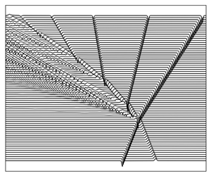
In the isopycnal waterfall plots presented below, the isopycnal at the centre of the upper pycnocline is used. The upper pycnocline is chosen because for all stratifications considered the linear mode-one eigenfunction has its maximum in the upper pycnocline so vertical displacements for linear waves are larger in the upper pycnocline than in the lower pycnocline. Hence, use of this isopycnal, rather than one in the lower pycnocline, makes it easier to see small-amplitude waves generated by the interaction of the two ISWs. In ISWs of depression the upper pycnocline undergoes a larger displacement than the lower pycnocline does but the opposite is true of ISWs of elevation. Hence the amplitude of ISWs of elevation is under-represented by the use of this isopycnal for the waterfall plots. This under-representation is illustrated in the density contour plots presented below.

5.1. Stratification $S_1$

We first consider the stratification $S_1$ for which $(z_1,z_2) = (-0.25, -0.9)$ and $\Delta \rho _1 = 0.55$ (table 1, figure 1). The stratification is indicated by a solid circle in figure 5(a) and the amplitude and propagation speed of ISWs as a function of APE are presented in figure 6. Here ISWs of elevation exist with a minimum amplitude of 0.210.

Figure 7 shows waterfall plots for four cases using this stratification. In figure 7(a) the interaction of two ISWs of KdV polarity (Case $C_1$, table 2) is shown. Their initial APEs are $0.04$ and $0.01$. The initial wave amplitudes (extreme isopycnal displacements) are $-0.140$ and $-0.231$ (figure 6) and these are also the initial displacements of the isopycnal at the centre of the upper pycnocline. At the scale of this waterfall plot there is no evidence of any additional waves being generated by the interaction; however, some small waves are generated with amplitude 0.0008 which is 0.6 % of the amplitude of the smaller initial ISW (see figure 8). At $t=7000$ the extreme isopycnal displacements in the two ISWs are $-0.139$ and $-0.230$, i.e. a decrease in amplitude by 0.7 % and 0.4 %. For comparison, in a simulation with only the single large wave its amplitude decreased by 0.2 % during the same time period due to numerical dissipation and a slight adjustment of the initial DJL ISWs. The interaction is similar to that of KdV solitary waves with amplitudes that are not too different: during the interaction the larger wave decreases in amplitude and slows down while the wave ahead of it grows and speeds up. There are always two local minimums in the isopycnal displacements. The interaction of these two solitary waves is very soliton-like, similar to the interactions of ISWs in an exponential stratification reported by Lamb (Reference Lamb1998).

Figure 7.

Waterfall plots showing the time evolution of the isopycnal at the centre of the upper pycnocline. Stratification $S_1$ with $(z_1,z_2) = (-0.25, -0.9)$ and $\Delta \rho _1 = 0.55$. (a) Case $C_1$: interaction of two solitary waves of KdV polarity with APEs of 0.01 (amplitude $-0.140$) and 0.04 (amplitude $-0.231$). (b) Case $C_2$: interaction of two solitary waves of negative KdV polarity with APEs of 0.02 (amplitude $0.258$) and 0.05 (amplitude $0.351$). (c) Case $C_3$: interaction of a fast wave of negative KdV polarity with APE of 0.05 (amplitude 0.351) with a slow wave of KdV polarity with APE of 0.002 (amplitude $-0.059$). (d) Case $C_4$: interaction of a fast wave of KdV polarity with APE of 0.003 (amplitude $-0.075$) with a slow wave of negative KdV polarity with APE of 0.03 (amplitude 0.301). Isopycnal displacements are scaled identically in all cases. The amplitude of the negative polarity waves (waves of elevation) is under-represented because of the use of the upper pycnocline.

Figure 8.

Zoom in on the isopycnal at the centre of the upper pycnocline at $t=4500$ for case $C_1$ (same case shown in figure 7a). Small-amplitude linear dispersive waves generated by the interaction lie between $x=-60$ and $-30$.

Figure 7(b) shows the interaction of two ISWs of negative KdV polarity for the same stratification (Case $C_2$). Their initial APEs are $0.02$ and $0.05$ with amplitudes of 0.258 and 0.351 (figure 6, table 2). The interaction generates a much larger trailing wave train and a small-amplitude solitary wave both of which can be seen in the waterfall plot. The displacement of the centre of the upper pycnocline decreases by 0.5 % and 1.9 % for the large and small ISWs respectively.

The interaction of two solitary waves of opposite polarity (Case $C_3$; see figure 6, table 2) with the fast wave being a wave of negative KdV polarity is shown in figure 7(c). The negative KdV polarity wave has an APE of 0.05 (amplitude 0.351) while the KdV polarity wave has an APE of 0.002 (amplitude $-0059$). A few small waves are generated by the interaction which is again soliton-like. The displacement of the upper pycnocline decreases by about 8 % and 0.9 % for the KdV and negative KdV polarity waves respectively.

When the slow and fast waves are negative KdV and KdV polarity waves, respectively, the results are quite different. An example, Case $C_4$ (see figure 6, table 2), is shown in figure 7(d). The initial faster-propagating wave of depression centred at $x = 30$ is a small-amplitude wave of KdV polarity (APE 0.003, amplitude $-0.0746$). The wave of elevation ahead of it at $x = 60$ has negative KdV polarity and is larger (APE 0.03, amplitude $0.3008$). The interaction results in the generation of a much larger-amplitude wave train than in the previous three cases. A striking result of the interaction is that the KdV polarity ISW undergoes a large increase in amplitude. It increases its amplitude by 113.1 % while the negative polarity ISW decreases its amplitude by 14.0 %. The energy of the KdV polarity wave (KE plus APE) increases by a factor of 4.43 from 0.0062 to 0.0273 while the energy of the negative polarity wave decreases by a factor of 0.53 from 0.0646 to 0.0340. The combined energy in the two ISWs has decreased by about 13.4 %. Approximately 9 % of the decrease is due to transfer of energy to the smaller trailing waves and the remaining 4.4 % is loss due to numerical dissipation (next section). An accompanying change in the propagation speeds of the two ISWs is evident. This change is exaggerated in the waterfall plot because of the use of a moving reference frame. Relative to the fluid the propagation speed of the KdV polarity wave increases by 5 % while the propagation speed of the negative KdV polarity wave decreases by 4 %.

Figure 9 shows contour plots of the density field before and after the interaction for Case $C_4$. This plot illustrates how displacements of the upper pycnocline can greatly under-represent the amplitude of the waves of elevation. It also illustrates that isopycnal displacements in the trailing wave train are larger in the upper pycnocline.

Figure 9.

Density contour plot of the interaction of two solitary waves of opposite polarities. Case $C_4$ (see figure 7d). (a) Shortly before the interaction at $t=4000$. (b) After the interaction at $t=6000$.

5.2. Stratification $S_2$

The second stratification considered has $(z_1,z_2) = (-0.15,-0.9)$ and $\Delta \rho _1 = 0.6$ (table 1, figure 5a). Compared with stratification $S_1$, the upper pycnocline has been raised and slightly strengthened with a corresponding decrease in the strength of the lower pycnocline. This stratification is indicated by a solid circle in figure 5(a). As for stratification $S_1$, KdV polarity waves are waves of depression and negative polarity waves of elevation exist, this time with a minimum amplitude of 0.144.

The interaction of two ISWs of KdV polarity or two waves of negative KdV polarity is similar to those for the previous stratification. Here we consider the interaction of two ISWs of opposite polarity (Case $C_5$, table 2) with a KdV polarity ISW (${\rm APE} = 0.01$, $a=-0.174$, $c=0.341$) initially trailing a slower-propagating negative KdV polarity ISW (${\rm APE} = 0.03$, $a=0.328$, $c=0.303$) as in Case $C_4$. A waterfall plot illustrating the interaction is presented in figure 10(a). The interaction is much more complicated than it was in Case $C_4$. As in Case $C_4$, the KdV polarity ISW increases its amplitude and propagation speed during the interaction while the negative KdV polarity wave undergoes a reduction in amplitude and propagation speed. The interaction generates several other waves including a KdV polarity solitary wave of depression which initially trails the negative KdV polarity ISW. Its propagation speed is negative in this reference frame. Relative to the fluid it is travelling faster than the negative KdV polarity wave so it catches up and interacts with it. During the interaction its amplitude increases and it then propagates to the right. A new packet of small-amplitude waves and a new KdV polarity ISW are produced. This cycle repeats several times. After each interaction the negative KdV polarity wave decreases in amplitude and each subsequent new KdV polarity ISW is smaller than the preceding one. After the third interaction of ISWs of opposite polarity (at $t\approx 1800$) the KdV polarity ISW is drifting to the left as its propagation speed relative to the fluid is smaller than the speed of the moving reference frame. Contour plots of the density field at three different times are presented in figure 11. A movie for this case is provided in the supplementary movie (movie 1) available at https://doi.org/10.1017/jfm.2023.284.

Figure 10.

Waterfall plots showing the time evolution of the isopycnal at the centre of the upper pycnocline. (a) Case $C_5$. Stratification $S_2$ with $(z_1,z_2) = (-0.15, -0.9)$ and $\Delta \rho _1 = 0.6$. (b) Case $C_6$. Interaction of two solitary waves of opposite polarities for the symmetric stratification $S_3$ with $(z_1,z_2) = (-0.1, -0.9)$ and $\Delta \rho _1 = 0.5$. Waves have APEs of $0.005$ (amplitude 0.1602) and $0.02$ (amplitude $-0.2754$).

Figure 11.

Density contour plot of the interaction of two solitary waves of opposite polarities. Case $C_5$ (see figure 10a). (a) Before the first interaction at $t=600$. (b) Second interaction at $t=1200$. (c) Third interaction at $t=1800$.

6. Energy considerations

The use of a second-order finite-volume method to solve the governing equations implies the presence of numerical damping and a gradual loss of energy from the wave field. This is illustrated in figure 12 where the time evolution of the total APE, KE and half the total energy in the computational domain is shown for Case $C_3$. The total energy decreases linearly in time until $t\approx 6000$ when waves in the wave train generated by the interaction (which occurs at about $t = 5200$) start to leave the domain (see figure 7c). During the interaction the KE undergoes a sharp, transient decrease while the APE has a corresponding sharp, transient increase. They recover somewhat but the total KE and APE undergo a permanent decrease and increase respectively after the interaction. The total energy shows no such behaviour, continuing to decrease at the same rate during the interaction.

Figure 12.

Time evolution of energy in the computational domain for Case $C_3$. Shown are the APE (red), KE (blue) and half the total energy (green).