


Introduction
Throughout the history of life on Earth, the vast majority of species to have ever existed have become extinct. Among those extinct species and lineages is to be found a staggering diversity of body forms, sizes, functions, and ecologies that have no counterpart in the modern day. Today there are no gargantuan terrestrial, aquatic, or aerial arthropods of the scale seen in the Paleozoic (Braddy et al. Reference Braddy, Poschmann and Tetlie2008); extant marine reptiles present only a fraction of the highly diverse phenotypes that existed in the Mesozoic (Sues Reference Sues2019); no modern habitat sustains the number or size of terrestrial herbivores as some evidently did in the Jurassic (Foster Reference Foster2007); there are no 10-tonne bipeds alive today (Hutchinson et al. Reference Hutchinson, Bates, Molnar, Allen and Makovicky2011); and the list goes on. Additionally, the myriad species that bridge the anatomical, physiological and ecological divide between disparate major clades today, such as “fishapods” (stem tetrapods), “mammal-like reptiles” (nonmammalian synapsids) “protobirds” (nonavian theropods), and “protowhales” (archaeocete artiodactyls) are absent from modern environments (Kemp Reference Kemp2016). It therefore comes as little surprise that research into the paleobiology of these enigmatic extinct species is a long-lived and still-growing field.
Underpinning many aspects of paleobiological research is the concept of uniformitarianism (Hutton Reference Hutton1788), that certain principles and phenomena observed in the modern day have always been in action across time and space. The laws of the physical world are one such set of principles, which lend to the investigation of biological aspects that are influenced and constrained by physics, that is, biomechanics. The investigation of biomechanical phenomena in paleobiological enquiry has a long history, and at least some aspect of biomechanics has been explored in every extinct vertebrate and many invertebrate groups (Thompson Reference Thompson1917; Alexander Reference Alexander1989; Thomason Reference Thomason1995). However, one group in particular has received prolonged and intensive attention in this field of study: the dinosaurs, which indeed continue to lead the charge in the development and application of new biomechanical approaches to the fossil record.
The intersection of dinosaur paleontology and biomechanics can be reciprocally illuminating; not only can biomechanics shed insight into how dinosaurs functioned as living animals (Alexander Reference Alexander1985, Reference Alexander1989, Reference Alexander2006a; Henderson Reference Henderson, Brett-Surman, Holtz and Farlow2012), but dinosaurs have much to offer the field of biomechanics, too. As some of the most successful vertebrates in history, they included the largest terrestrial animals to ever exist, for both quadrupeds and bipeds (Colbert Reference Colbert1962; Hutchinson et al. Reference Hutchinson, Bates, Molnar, Allen and Makovicky2011; Campione and Evans Reference Campione and Evans2012; Campione et al. Reference Campione, Evans, Brown and Carrano2014; Bates et al. Reference Bates, Mannion, Falkingham, Brusatte, Hutchinson, Otero, Sellers, Sullivan, Stevens and Allen2016, Benson et al. Reference Benson, Hunt, Carrano and Campione2018); exhibited repeated evolutionary increases and decreases in body size (Sereno Reference Sereno1999; Carrano Reference Carrano, Carrano, Gaudin, Blob and Wible2006; Turner et al. Reference Turner, Pol, Clarke, Erickson and Norell2007; Benson et al. Reference Benson, Hunt, Carrano and Campione2018) and transitions from bipedal to quadrupedal posture (Charig Reference Charig, Joysey and Kemp1972; Carrano Reference Carrano, Curry Rogers and Wilson2005; Maidment and Barrett Reference Maidment and Barrett2012, Reference Maidment and Barrett2014; Maidment et al. Reference Maidment, Henderson and Barrett2014c); and displayed substantial disparity in cranial and postcranial anatomy with attendant functional differences (Rayfield Reference Rayfield2005; Hutchinson and Allen Reference Hutchinson and Allen2009; Maidment et al. Reference Maidment, Bates, Falkingham, VanBuren, Arbour and Barrett2014b; Button and Zanno Reference Button and Zanno2020); one lineage evolved an additional mode of locomotion, powered flight (Ostrom Reference Ostrom1976; Gauthier and Padian Reference Gauthier and Padian1985; Gatesy Reference Gatesy, Chiappe and Witmer2002; Gauthier and Gall Reference Gauthier and Gall2002; Heers and Dial Reference Heers and Dial2012); and an increasing array of taxa are suspected of having undergone substantial change in functional abilities during ontogeny (e.g., Heinrich et al. Reference Heinrich, Ruff and Weishampel1993; Dilkes Reference Dilkes2001; Currie Reference Currie2003; Carr and Williamson Reference Carr and Williamson2004; Hutchinson et al. Reference Hutchinson, Bates, Molnar, Allen and Makovicky2011; Otero et al. Reference Otero, Cuff, Allen, Sumner-Rooney, Pol and Hutchinson2019). These aspects, combined with the dinosaurs’ long evolutionary history (>160 million years) and rich fossil record, mean that dinosaurs can be viewed as a “natural laboratory” for testing the generality of biomechanical principles derived from studies of extant species (Biewener Reference Biewener1989; Alexander Reference Alexander2006b). Indeed, careful study of the extremes in body form and function in dinosaurs could well lead to extensions to current biomechanical principles based on extant species. Framed in a comparative context, dinosaur paleontology can therefore add a novel dimension to biomechanical enquiry—that of “deep time” (Hutton Reference Hutton1788), one which is beyond the familiar temporal scales of most biomechanists, and yet one which is intricately linked to the anatomical system in question through the process of evolution (Darwin Reference Darwin1859; Taylor and Thomas Reference Taylor and Thomas2014).
Nevertheless, this great opportunity comes with a variety of challenges, which ultimately stem from the fact that almost all dinosaurs (along with all other extinct species) are known only from static and often incomplete fossilized remains. In this paper, we outline an approach that we, as paleontologists, biomechanists, and evolutionary biologists, have refined over many years to surmount one aspect of the challenge of integrating dinosaur paleontology and biomechanics: that of reconstructing locomotor biomechanics. A wide variety of methods have been employed in the past for inferring how a given dinosaur locomoted, including those grounded in comparison to extant terrestrial vertebrates (Bakker Reference Bakker1971; Alexander Reference Alexander1976, Reference Alexander1985, Reference Alexander1989; Coombs Reference Coombs1978; Paul Reference Paul1988; Gatesy and Middleton Reference Gatesy and Middleton1997; Carrano Reference Carrano2001; Moreno et al. Reference Moreno, Carrano and Snyder2007), and vary across the continuum from purely qualitative through to extensively quantitative. We do not review them here, and direct the reader to Hutchinson and Gatesy (Reference Hutchinson and Gatesy2006) and Henderson (Reference Henderson, Brett-Surman, Holtz and Farlow2012) for useful introductions to the topic, as well as Hutchinson (Reference Hutchinson2012) and Anderson et al. (Reference Anderson, Bright, Gill, Palmner and Rayfield2012) for more general introductions to the integration of biomechanical models in paleontology. Rather, we aim here to use dinosaurs as a vehicle for demonstrating how a careful, structured, and quantitative approach can maximize the rigor of the entire process of reconstructing locomotor biomechanics in extinct animals, and in turn maximize the robustness of the end results. Such methodology can also help identify inherent strengths and limitations, and therefore paves the way for future progress.
Our approach involves the explicit application of quantitative biomechanical principles that are derived from well-known and fundamental physical laws. This methodology offers a unique level of quantitative rigor that facilitates transparency and repeatability and provides a route to a more direct, mechanistic understanding of the underlying phenomena. We progress from fossil bones to digital articulated skeletons, and thence to “fleshed-out” reconstructions of the whole animal (in terms of both external geometry and internal musculature), and finally to the development of models and simulations based upon these reconstructions. As a case study to demonstrate each step in the workflow, we use the small, Late Triassic theropod Coelophysis bauri, focusing on the hindlimb in locomotion. This forms a contrast to many prior studies of giant Jurassic or Cretaceous forms like Tyrannosaurus, Allosaurus, and Acrocanthosaurus (e.g., Hutchinson and Garcia Reference Hutchinson and Garcia2002; Henderson and Snively Reference Henderson and Snively2003; Hutchinson et al. Reference Hutchinson, Anderson, Blemker and Delp2005, Reference Hutchinson, Bates, Molnar, Allen and Makovicky2011; Bates et al. Reference Bates, Falkingham, Breithaupt, Hodgetts, Sellers and Manning2009a,Reference Bates, Manning, Hodgetts and Sellersb, Reference Bates, Benson and Falkingham2012a; Sellers et al. Reference Sellers, Pond, Brassey, Manning and Bates2017) and provides a new perspective on how this bipedal taxon may have stood and moved (Colbert Reference Colbert1989; Padian and Olsen Reference Padian, Olsen, Gillette and Lockley1989; Gatesy et al. Reference Gatesy, Middleton, Jenkins and Shubin1999; Hutchinson Reference Hutchinson2004b; Allen et al. Reference Allen, Bates, Li and Hutchinson2013). Despite our taxonomic focus, the workflow detailed herein is broadly applicable to the study of locomotor biomechanics in many groups of extinct vertebrates beyond nonavian dinosaurs, although case-specific nuances will often require practical modifications. At each step, we advocate what we believe to be the current best practice for maximizing data utility and robustness of results.
Methods and Results
Rather than present the techniques first and then new results obtained, here we combine the methods and findings. The reconstruction of locomotor biomechanics in a given extinct vertebrate is typically an iterative approach, wherein preliminary results obtained may signal the need for improvement in the reconstruction or modeling methodology, and therefore results can help inform methods and vice versa (see also Hicks et al. Reference Hicks, Uchida, Seth, Rajagopal and Delp2015). Such reciprocal illumination is not a case of circularity, however; so long as clear questions and standards are defined at the outset, this self-refining “total evidence” perspective can help improve the precision with which a given question is answered, maximize the robustness of results, and increase the study's transparency and repeatability. Our workflow involves the following key steps (Fig. 1):
1. building digital models from three-dimensional (3D) imaging of the original fossil specimens;
2. articulating digital bones together in jointed skeletons;
3. delimiting joint mobility;
4. calculating the 3D shape and dimensions of the whole body and its individual segments;
5. reconstructing the attachments of soft tissues such as muscles or ligaments;
6. quantifying the geometry of muscle paths;
7. estimating aspects of muscle anatomy or physiology that influence force production; and
8. using computational models for simulation and hypothesis testing of locomotor function, behavior and performance.
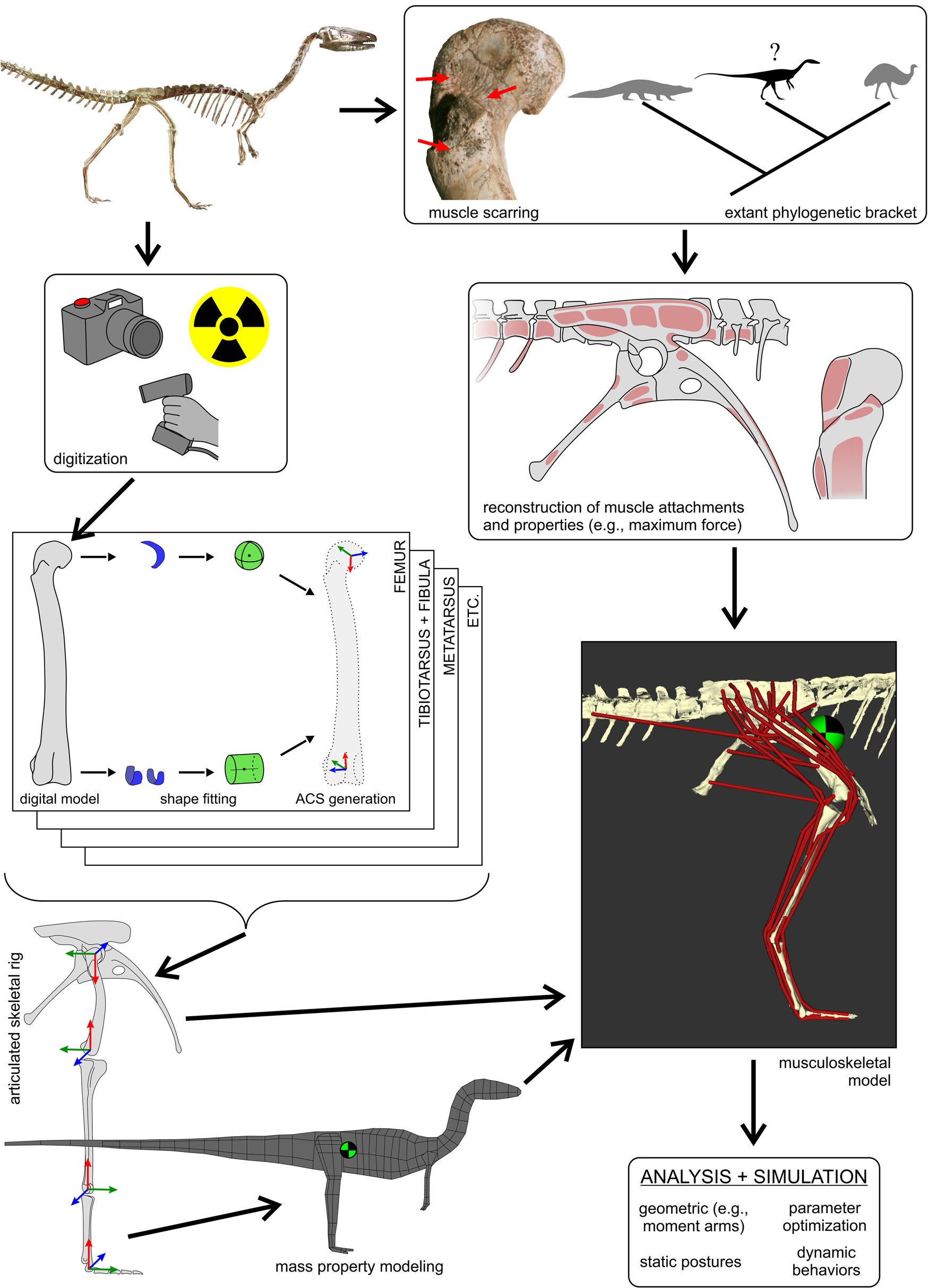
The overall workflow followed to generate three-dimensional (3D) musculoskeletal models of fossil taxa, in this case, Coelophysis. This figure schematically highlights the main steps involved, with further detail provided in the text and following figures. The 3D geometry of the fossil bones is digitally captured using a variety of modalities, including photogrammetry, computed tomography (X-ray or otherwise) and laser surface scanning. These geometries are used to determine joint centers (via shape-fitting algorithms) and in turn derive anatomical coordinate systems (ACSs) for each bone. The bones can then be precisely articulated into a rigid hierarchical framework that serves as a basis upon which to estimate mass properties, namely mass, center of mass location (checkered disk), and the inertia tensor. Combined with reconstructed muscle attachments and inference of muscle lines of action, this is used to produce a digital musculoskeletal model. Intrinsic physiological properties of each muscle (e.g., maximum isometric force, F max) may also be estimated from muscle-tendon unit dimensions or inference from extant bracketing taxa. The fully defined musculoskeletal model then provides the basis for a wide range of analyses and simulations. Photograph of mounted skeleton at the Cleveland Museum of Natural History courtesy of C. Griffin.
The ambiguity that surrounds a given unknown (and frequently unknowable) parameter, and in turn how this may affect the cascade of higher-level inferences (Witmer Reference Witmer and Thomason1995; Bates and Falkingham Reference Bates and Falkingham2018), can be more explicitly addressed through the use of this structured, hierarchical approach. It is also worth noting that, given the uncertainties associated with fossil organisms, our perspective on hypothesis testing is not one of determining “the” answer, as may sometimes seem to be the case in biomechanical studies of extant species. Instead, we seek to determine what the answer could not have been, and thereby rule out impossible and implausible solutions; what remains of the solution space after all tests have been conducted remains the realm of plausibility, subject to future testing (Blob Reference Blob2001; Gatesy et al. Reference Gatesy, Bäker and Hutchinson2009; Nyakatura et al. Reference Nyakatura, Melo, Karakasiliotis, Allen, Andikfar, Andrada, Arnold, Lauströer, Hutchinson, Fischer and Ijspeert2019).
Acquiring Digital Fossil Morphology
The first step involves transcribing the real, physical morphology of a fossil into a digital facsimile that is of sufficiently high accuracy to serve the purposes of biomechanical investigation. How this is done, and the accuracy (detail) with which the digital model represents the original specimen, will vary depending on the specific question being addressed. There are many modalities to generating 3D digital facsimiles of skeletal elements, and common methods include computed tomographic scanning, photogrammetry, laser scanning, and point digitizing. Useful introductions to these (and other) methods and their practical nuances are given by Cunningham et al. (Reference Cunningham, Rahman, Lautenschlager, Rayfield and Donoghue2014) and Sutton et al. (Reference Sutton, Rahman and Garwood2017). As the availability and performance of these methods continues to increase, it is also important to consider the logistical implications of storage and accessibility of increasingly large volumes of digital data long-term, for the sake of data integrity and research reproducibility (Boyer et al. Reference Boyer, Gunnell, Kaufman and McGeary2017; Davies et al. Reference Davies, Rahman, Lautenschlager, Cunningham, Asher, Barrett, Bates, Bengtson, Benson, Boyer, Braga, Bright, Claessens, Cox, Dong, Evans, Falkingham, Friedman, Garwood, Goswami, Hutchinson, Jeffery, Johanson, Lebrun, Martínez-Pérez, Marugán-Lobón, O'Higgins, Metcher, Orliac, Rowe, Rücklin, Sánchez-Villagra, Shubin, Smith, Starck, Stringer, Summers, Sutton, Walsh, Weisbecker, Witmer, Wroe, Yin, Rayfield and Donoghue2017), as well as how this may integrate with data archiving and sharing policies of the institutions in which the physical specimens are housed.
We advocate capturing morphology at a higher level of detail than what may be considered the bare minimum required, as this can prove useful (even necessary) for future refinement. If the generated dataset is too large for the current study—for example, data files are too large for efficient computational processing or analysis—it can always be downsampled (with decreased detail), but a low-resolution dataset cannot be upsampled to increase detail.
A high-resolution dataset may also serve a use for other, unrelated studies by the same or other research groups; obviating the need to redigitize a specimen saves time and also helps minimize the potentially harmful handling of fragile fossils during the digitization process.
Fossil specimens have often suffered taphonomic distortion, and while it is obviously desirable to work with undistorted material, this may not be an option in the case of unique specimens. The type and magnitude of taphonomic distortion may influence the results of biomechanical analysis (e.g., if finite element methods are to be used in a structural analysis), and if this is deemed to be the case, then retrodeformation and reconstruction can be used to help restore in vivo morphology (e.g., Molnar et al. Reference Molnar, Pierce, Clack and Hutchinson2012; Tallman et al. Reference Tallman, Amenta, Delson, Frost, Ghosh, Klukkert, Morrow and Sawyer2014; Cuff and Rayfield Reference Cuff and Rayfield2015; Lautenschlager Reference Lautenschlager2016; Vidal and Díaz Reference Vidal and Díaz2017), although it is possible that no retrodeformation technique can fully restore the original, true morphology (Hedrick et al. Reference Hedrick, Schachner, Rivera, Dodson and Pierce2019). Missing elements, or parts thereof, can be “filled in” from other elements, be it the contralateral antimere (mirroring right–left), neighboring serial homologue (as in the case of vertebrae) or from another individual of the same or closely related species. These all come with levels of uncertainty that may be markedly higher for elements that lack an axis of symmetry, such as limb bones. When important components of the final skeletal model are generated through retrodeformation or “filling in,” sensitivity analysis may be required to improve confidence that possible errors will not have significant effects on downstream results, or at least that these effects can be contained and handled appropriately. For example, could reconstructing the missing or deformed bone(s) in a different way have an important effect on the size or shape of part of the body? Of course, it is up to the investigator to decide which, if any, aspects are uncertain enough to warrant sensitivity analysis, and what level of downstream error is acceptable; this also needs to be weighed against what is practically feasible to do (lest a never-ending sensitivity analysis cycle occurs). Whichever is decided, we encourage explicit documentation and mechanistic justification of these decisions to maximize transparency.
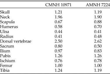
The reconstructed Coelophysis skeleton used in the present study was based on that of Allen et al. (Reference Allen, Bates, Li and Hutchinson2013), which was derived from laser scan data of a composite mounted skeleton at the Cleveland Museum of Natural History (CMNH 10971). We had concerns over the accuracy of this composite, and so the proportions were compared with photogrammetric models made of specimens in the American Museum of Natural History (AMNH): the neotype (AMNH 7224), the paired specimen (AMNH 7223), and AMNH block IX containing multiple individuals (including AMNH 7227–7231, 7234, 7236, and parts of other individuals). The pre-sacral proportions of CMNH 10971 (relative to femur length) are similar to those in AMNH 7224 (Table 1). However, there is uncertainty over the tails of both AMNH 7223 and 7224 (only partial tails were figured in the original photographs curated at the AMNH; see Nesbitt et al. Reference Nesbitt, Turner, Erickson and Norell2006), so the post-sacral elements were compared with AMNH 7229 from block IX, which comprises a complete tail and pelvis. The tail in the composite model is approximately 30% shorter than expected from the other bone lengths, with the “missing length” derived principally from the thin, distal end. The foreshortened tail in our model is not expected to have any important influence on the results; because the extremely small amount of mass in the missing distal end would shift the whole-body center of mass (see “Reconstructing Body Shape and Dimensions”) only slightly caudally (see eq. 1 of Allen et al. Reference Allen, Bates, Li and Hutchinson2013), the posture required for stability and commensurate required muscular effort would not change appreciably.
Pre-sacral proportions in the composite specimen used as the basis of the Coelophysis model (CMNH 10971) compared with those of the neotype (AMNH 7224), expressed as lengths relative to femur length. Ordinary least squares regression of the two datasets has an r 2 of 0.957.
Articulating Digital Skeletons
Depending on the mode of fossil digitization and research goals, digital bone models may be articulated “as is” from mounted specimens or manually by using knowledge of comparative anatomy. However this is done, we advocate using a precise, quantitative procedure that easily facilitates comparison with other species and studies, and that this procedure be thoroughly documented. Here we describe one approach for semi-automated and precise articulation of bone models that is objectively based on the morphology at hand (Fig. 2), borrowing from techniques used in prior studies of extant animal locomotion (Grood and Suntay Reference Grood and Suntay1983; Rubenson et al. Reference Rubenson, Lloyd, Besier, Heliams and Fournier2007; Miranda et al. Reference Miranda, Rainbow, Leventhal, Crisco and Fleming2010; Kambic et al. Reference Kambic, Roberts and Gatesy2014). This involves establishing anatomical coordinate systems (ACSs) for each bone involved and articulating them via a defined convention to create joint coordinate systems (JCSs), which can then be used to pose skeletons and describe postures in a consistent, quantitative fashion.
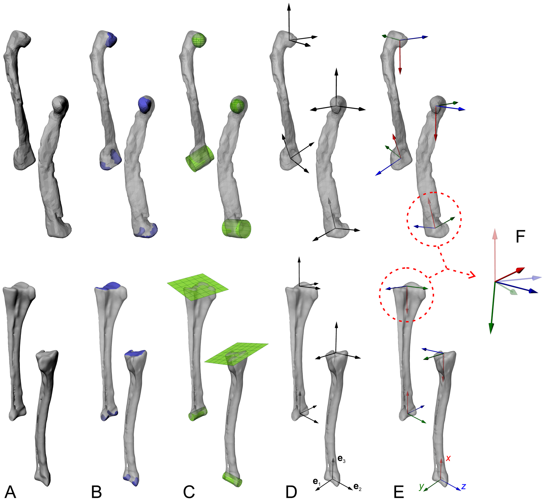
Objective determination of anatomical and joint coordinate systems (ACSs and JCSs, respectively), with the femur and tibiotarsus + fibula as an example. Each bone is shown in anterolateral and anteromedial views for each step. A, The digitized geometry of the whole bone. B, The joint articular surfaces are isolated. C, Geometric primitives are fit to the surfaces, to derive joint centers and, in the case of cylinders, joint axes. D, Information from the fitted shapes, and possibly from the bone model's inertia tensor, is used to derive three mutually orthogonal vectors (e1, e2, e3) at each end. E, Anatomical or functional meanings are assigned to produce a right-handed ACS at the end of each bone. F, ACSs from neighboring bones are articulated to form a JCS, which describes the disposition (rotations and/or translations) of a “child” ACS (solid) relative to a “parent” ACS (translucent); e.g., a knee JCS describes the proximal crus ACS relative to the distal femoral ACS. Each JCS follows a consistent rotation order; here we follow Kambic et al. (Reference Kambic, Roberts and Gatesy2014) and others in using a z–y′–x″ convention, corresponding to flexion–extension, abduction–adduction, and long-axis rotation, respectively. Note that while the femoral diaphysis in this example exhibits significant taphonomic crushing, such deformation is absent in the ends of the bones the shapes are fit to; in the context of musculoskeletal modeling, this form of distortion is of no concern. However, taphonomic distortion may modify the disposition of the two ends relative to each other (e.g., twisting, affecting the calculation of ACSs).
As a repeatable and objective way of establishing bone ACSs, geometric primitives such as spheres, ellipsoids, cylinders, and planes are fit to the articular surfaces at the joints, to compute aspects such as joint centers and primary axes (Li et al. Reference Li, Abram, Beaudoin, Berthiaume, Pelletier and Martel-Pelletier2008; Miranda et al. Reference Miranda, Rainbow, Leventhal, Crisco and Fleming2010; Kambic et al. Reference Kambic, Roberts and Gatesy2014). This first requires that the area of the articular surfaces involved is delimited, so that the geometric primitive is fit only to that part of the bone (Fig. 2B); this may in turn require that the bone model be “trimmed” to remove all non-articular surface geometry beforehand, which can be accomplished in many software packages, including open-source packages such as MeshLab (Cignoni et al. Reference Cignoni, Callieri, Corsini, Dellepiane, Ganovelli and Ranzuglia2008) and Blender (Blender Community 2018). We recommend selecting only that part of the bone inferred to have actually engaged in articulation in life, for example, only the surfaces covered by hyaline cartilage (but see Kambic et al. Reference Kambic, Roberts and Gatesy2014). The automated fitting of geometric primitives to the selected articular surface geometries can be performed in various software packages (e.g., Geomagic, 3D Systems, Inc., Rock Hill, S.C., U.S.A.; 3-matic, Materialise, Leuven, Belgium; Maya or 3ds Max, Autodesk, San Rafael, Calif., U.S.A. [free for educators, including academics]; Rhinoceros, McNeel, Seattle, Wash., U.S.A.), although often they are proprietary and the exact fitting algorithm used is undisclosed, which hampers comparison and repeatability across research groups. To address this, we have developed a set of code in MATLAB (MathWorks, Inc., Natick, Mass., U.S.A.) to perform rapid primitive fitting (Fig. 2C), and provide the complete code in the Supplementary Material (https://doi.org/10.5061/dryad.73n5tb2v9), documenting the underlying algorithms used. The code has been extensively tested on a wide range of morphologies drawn from extant and extinct archosaur bones, and we encourage others to test it in their own applications. Compared with prior studies that involved manual alignment of 2D or 3D shapes to joint surfaces (e.g., Hutchinson et al. Reference Hutchinson, Anderson, Blemker and Delp2005; Costa et al. Reference Costa, Rocha-Barbosa and Kellner2014; Brassey et al. Reference Brassey, Maidment and Barrett2017; Lai et al. Reference Lai, Biewener and Pierce2018), we contend that the repeatability that comes with using a quantitative, optimization-based procedure to shape fitting represents an improvement in methodological objectivity. Nevertheless, subjectivity remains in the selection of articular surface areas to fit geometric primitives to, especially if it is not clear where articular surfaces on the fossil bone start and end (e.g., in poorly preserved or ossified specimens). Additionally, some joint surfaces (e.g., glenoid of the shoulder girdle) may not bear close resemblance to any idealized geometric primitive, which adds the further complexity of which primitive to fit in the first instance. Sensitivity analysis can help clarify the potential magnitude of downstream effects resulting from differing surface selections and choice of primitive fitting (e.g., Demuth et al. Reference Demuth, Rayfield and Hutchinson2020), although again this needs to be weighed against what is practically feasible and, in comparative studies, the potential need to remain consistent across disparate morphologies.
The mathematical aspects of the fitted geometries (centers, axes, etc.) are then used to objectively establish sets of three mutually perpendicular, unnamed axes (e1, e2, e3) using the cross (vector) product (Fig. 2D) (Kambic et al. Reference Kambic, Roberts and Gatesy2014; Bishop et al. Reference Bishop, Hocknull, Clemente, Hutchinson, Farke, Beck, Barrett and Lloyd2018d). These axes are created in relevant parts of the bones or segments. Principal axes of inertia calculated from the digital model of a whole bone may also be used in the generation of these unnamed axes; for example, the axis of least inertia may grossly correspond to a limb bone's long axis (e.g., Kambic et al. Reference Kambic, Roberts and Gatesy2014), and thereby be useful. Anatomical and functional significance is then assigned to the axes, to form a right-handed ACS (Fig. 2E); the attitude of the ACS (i.e., the direction of the x-, y-, and z-axes) will vary depending on the anatomical system under study and the research question. Regardless of the rotation sequence that is used to describe joint movement, it is usually desirable to set the first axis of rotation to correspond with the axis of greatest anticipated range of motion in the joint (Brainerd et al. Reference Brainerd, Baier, Gatesy, Hedrick, Metzger, Gilbert and Crisco2010; Nyakatura and Fischer Reference Nyakatura and Fischer2010; Baier and Gatesy Reference Baier and Gatesy2013; Kambic et al. Reference Kambic, Roberts and Gatesy2014; Otero et al. Reference Otero, Allen, Pol and Hutchinson2017; Bishop et al. Reference Bishop, Hocknull, Clemente, Hutchinson, Farke, Barrett and Lloyd2018c).
Following ACS creation, bones are articulated in a hierarchical “marionette” (Gatesy et al. Reference Gatesy, Baier, Jenkins and Dial2010; Pierce et al. Reference Pierce, Clack and Hutchinson2012), comprising nested parent–child relationships between adjacent bones or segments. For instance, the pelvis forms the parent to the femur, which in turn forms the parent to the tibia and fibula, and so on. Software packages in which this can be done include Maya, 3ds Max, Rhinoceros, Blender, SIMM (Motion Analysis, Rohnert Park, Calif., U.S.A.) and OpenSim (Delp et al. Reference Delp, Anderson, Arnold, Loan, Habib, John, Guendelman and Thelen2007); Blender and OpenSim are also open-source. The translational and rotational offset of a child relative to its parent is described using a pair of ACSs to form a JCS; for instance, the knee JCS describes how the proximal tibia and fibula ACS is spatially related to the distal femur ACS (Fig. 2F). Mathematically, these spatial relations are most succinctly described using a 4 × 4 transformation matrix, but as this is abstract and not intuitive from a biological perspective, intrinsic (child body-fixed) Euler rotations are often used instead (see Winter Reference Winter2009). It is important to note that the order in which Euler rotations are performed is noncommutative, and therefore requires explicit documentation to facilitate comparisons across studies; in our work we use flexion–extension, followed by abduction–adduction, followed by long-axis rotation (pronation–supination), as per Kambic et al. (Reference Kambic, Roberts and Gatesy2014). The use of a JCS inherently involves a priori defining a point of reference from which translations or rotations are measured, that is, a “default,” “neutral,” or “reference” position at which all translations and rotations are zero. Again, how the neutral posture is defined may vary depending on the anatomical system under study and the research question.
In our Coelophysis model, ACSs were created at the acetabulae of the pelvis and at the proximal and distal ends of each limb segment (see Kambic et al. Reference Kambic, Roberts and Gatesy2014). To achieve this, spheres were fit to the acetabulum and femoral head; cylinders to the distal condyles of the femur, tibiotarsus, and distal metatarsal III; and planes to the proximal tibia + fibula, proximal metatarsus, and proximal phalanx III-3. Bones were articulated into a skeletal marionette in Maya and aligned into a neutral posture following Hutchinson et al. (Reference Hutchinson, Anderson, Blemker and Delp2005), where the limb (except phalanges) is vertically straightened, so that the long axis of a given limb segment points toward its proximal joint center. One exception to this was modeling the forelimbs with 90° of elbow flexion (cf. Allen et al. Reference Allen, Bates, Li and Hutchinson2013) to approximate a more lifelike pose for the purpose of our hindlimb-focused analyses. In articulating a skeletal marionette, assumptions of joint spacing may be required to account for missing intervening soft tissues such as cartilage (Pierce et al. Reference Pierce, Clack and Hutchinson2012; Arnold et al. Reference Arnold, Fischer and Nyakatura2014; Lai et al. Reference Lai, Biewener and Pierce2018; Regnault and Pierce Reference Regnault and Pierce2018; Tsai et al. Reference Tsai, Turner, Manafzadeh and Gatesy2020). Different methods of estimating joint spacing have been proposed, including scaling based on empirical data for extant relatives or setting spacing in direct relation to bony geometry. Our Coelophysis model was articulated with joint spacing following the same protocol for the Tyrannosaurus model of Hutchinson et al. (Reference Hutchinson, Anderson, Blemker and Delp2005), where the amount of space used is a set proportion of segment length (7.5% for femur, 5% for tibiotarsus, and 10% to the metatarsus); this was based on unpublished observations of joint spacing in extant archosaurs and is roughly similar to the detailed data presented by Holliday et al. (Reference Holliday, Ridgely, Sedlmayr and Witmer2010). No consensus has yet been reached as to which method of determining joint spacing is most appropriate, or whether different situations necessitate different methods. Additionally, we also suspect that the importance of joint spacing, and therefore whether it should be considered in sensitivity analyses, will differ depending on the spatial scale of the research question. For example, inferences of joint mobility (see “Assessing Joint Mobility”) will likely be more sensitive to joint spacing than inferences of whole-limb mechanics in locomotion, as animals rarely use the full range of joint motion in normal gait (Arnold et al. Reference Arnold, Fischer and Nyakatura2014; Kambic et al. Reference Kambic, Roberts and Gatesy2017).
Our research goals ultimately lie in musculoskeletal function (see “Musculoskeletal Simulation and Hypothesis Testing”), and so the marionette in Maya was then transcribed to the OpenSim modeling environment using a second set of custom MATLAB code, which we also provide in the Supplementary Material. As with many prior studies of extinct species, for the sake of simplicity, joints were permitted rotation only (Hutchinson et al. Reference Hutchinson, Anderson, Blemker and Delp2005, Reference Hutchinson, Miller, Fritsch, Hildebrandt, Endo and Frey2008; Bates and Schachner Reference Bates and Schachner2012; Bates et al. Reference Bates, Benson and Falkingham2012a; Sellers et al. Reference Sellers, Margetts, Coria and Manning2013, Reference Sellers, Pond, Brassey, Manning and Bates2017; Maidment et al. Reference Maidment, Bates, Falkingham, VanBuren, Arbour and Barrett2014b; Otero et al. Reference Otero, Allen, Pol and Hutchinson2017; Bishop et al. Reference Bishop, Hocknull, Clemente, Hutchinson, Farke, Barrett and Lloyd2018c; Nyakatura et al. Reference Nyakatura, Melo, Karakasiliotis, Allen, Andikfar, Andrada, Arnold, Lauströer, Hutchinson, Fischer and Ijspeert2019). This implicitly assumes that the joint centers themselves remain fixed with respect to the parent body during joint motion, which is probably a simplification for many joints and degrees of freedom (Baier and Gatesy Reference Baier and Gatesy2013; Hirschmann and Müller Reference Hirschmann and Müller2015; see also next section).
Assessing Joint Mobility
Previous investigations of behavior in many extinct vertebrate taxa frequently involve the quantitative assessment of range of motion and mobility in one or more joints (Padian and Olsen Reference Padian, Olsen, Gillette and Lockley1989; Paul Reference Paul1998; Senter and Robins Reference Senter and Robins2005; Senter Reference Senter2009; Mallison Reference Mallison2010a,Reference Mallisonb; Pierce et al. Reference Pierce, Clack and Hutchinson2012; Lai et al. Reference Lai, Biewener and Pierce2018). For clarity, we make a subtle distinction here: “range of motion” (ROM) refers to the quantitative bounds on movement about any single joint axis, whereas “mobility” considers motion about all axes together, in terms of both differences in ROM about different axes as well as how motion about one axis can influence that about another (see Kambic et al. Reference Kambic, Roberts and Gatesy2017). In the context of extinct species such analysis inherently can only work with the morphology of the fossil bones. Even if the bones themselves are excellently preserved, articular surface geometries may not faithfully reflect actual articular geometries in life due to missing cartilage (Bonnan et al. Reference Bonnan, Sandrik, Nishiwaki, Wilhite, Elsey and Vittore2010; Tsai and Holliday Reference Tsai and Holliday2015). In turn, this can introduce error in estimating in vivo joint spacing, which may have consequences for further downstream analyses; again sensitivity analysis (e.g., Lai et al. Reference Lai, Biewener and Pierce2018; Regnault and Pierce Reference Regnault and Pierce2018; Demuth et al. Reference Demuth, Rayfield and Hutchinson2020) may be warranted to delimit what these consequences could be. Coupled with other missing soft tissues that can influence joint mobility, such as ligaments, menisci, and even muscle and integument (Carpenter and Wilson Reference Carpenter and Wilson2008; Hutson and Hutson Reference Hutson and Hutson2012; Pierce et al. Reference Pierce, Clack and Hutchinson2012; Arnold et al. Reference Arnold, Fischer and Nyakatura2014; White et al. Reference White, Cook, Klinkhamer and Elliott2016; Manafzadeh and Padian Reference Manafzadeh and Padian2018; Tsai et al. Reference Tsai, Middleton, Hutchinson and Holliday2018, Reference Tsai, Turner, Manafzadeh and Gatesy2020), the results obtained from a “bones only” approach may significantly overestimate in vivo mobility. This long-recognized issue remains a key challenge to be overcome. Despite this, ROM assessments still have value in that they can help identify joint poses and limb postures that are infeasible, thereby delimiting the upper bounds of what a limb was potentially capable of doing (Gatesy et al. Reference Gatesy, Bäker and Hutchinson2009): in life, limb mobility was likely less. Depending on the question at hand, it is therefore the task of the researcher to use other methods that either constrain potential limb mobility further, or alternatively that more directly identify the postures actually used. In our workflow of building musculoskeletal models of the anatomical system in question, we use evidence drawn from muscle anatomy and leverage, bone structure (external or internal), and basic biomechanical principles to further “whittle down” probable limb pose space (see “Musculoskeletal Simulation and Hypothesis Testing”; Hutchinson et al. Reference Hutchinson, Anderson, Blemker and Delp2005; Gatesy et al. Reference Gatesy, Bäker and Hutchinson2009; Bishop et al. Reference Bishop, Hocknull, Clemente, Hutchinson, Farke, Barrett and Lloyd2018c).
For our nascent articulated Coelophysis model in the OpenSim environment, the ROM for each degree of freedom was determined as precisely as possible by manually rotating about each joint axis independently (with other axes held stationary) and using criteria such as joint surface disarticulation or bone-on-bone contact to identify joint limits (Fig. 3) (Senter and Robins Reference Senter and Robins2005; Carpenter and Wilson Reference Carpenter and Wilson2008; Paul Reference Paul, Larsen and Carpenter2008; Lai et al. Reference Lai, Biewener and Pierce2018). For hip flexion–extension and long-axis rotation, this was performed with abduction set at 15° (to bring the femur into a more parasagittal orientation from its neutral pose; see Fig. 3B). It was also assumed that the knee and ankle could not hyperextend beyond the straightened neutral pose, even though this was technically osteologically viable, as this was considered implausible based on the functional anatomy of extant archosaurs.
Joint convention definitions used and range of motion (ROM) for each joint in the hindlimb of Coelophysis, shown in both lateral (A) and anterior (B) views. Flexion and extension for all joints are presented in A, with hip abduction–adduction and long-axis rotation presented in B. In both panels, the neutral posture is shown opaque, with extremes of motion shown translucent. Inset boxes show instances of bone-on-bone contact used to identify limits to ROM.

An alternative approach is the use of an automated method, particularly that of Manafzadeh and Padian (Reference Manafzadeh and Padian2018), which can delimit ROM and mobility in a more objective and repeatable fashion. More importantly, automated assessment is more realistic, in that it can assess ROM across multiple degrees of freedom simultaneously, allowing for the interdependence of joint axes’ ROM limits to be reliably captured; thus, the true osteologically constrained mobility of the joint is measured. In some situations, joint morphology alone may not totally constrain in vivo ROM, as other parts of the body may exert “far-field” influences, such as the girth of the ribcage limiting the amount of femoral protraction (i.e., hip flexion). Regardless of whether a manual or automated method is employed, we advocate explicit documentation of the criteria used to assess ROM, as well as the precise axes about which ROM is measured. As interactions between rotational degrees of freedom may occur, imprecise definition of joint axes (if not using the ACS and JCS workflow outlined earlier) may conflate results from one axis with another, leading to kinematic “cross talk” (Rubenson et al. Reference Rubenson, Lloyd, Besier, Heliams and Fournier2007; Kambic et al. Reference Kambic, Roberts and Gatesy2014). The definitions of joint conventions and ROM for our Coelophysis model are presented in Figure 3. A considerably higher limit to maximal hip extension is ascribed to the present model compared with a previous assessment of this taxon (Padian and Olsen Reference Padian, Olsen, Gillette and Lockley1989), including the ability of the femur to extend beyond the vertical.
Most modeling environments, including OpenSim, describe the operation of each degree of freedom independent of one another, and hence ROM is determined for each joint axis independent of the others, with other axes typically set in their neutral configurations. This simplified approach ignores the potential interactions that can occur between different degrees of freedom in a joint (Kambic et al. Reference Kambic, Roberts and Gatesy2017; Manafzadeh and Padian Reference Manafzadeh and Padian2018). Moreover, for the sake of modeling simplicity in subsequent steps, it is customary to limit some joints to certain degrees of freedom only. A further point worth noting is that, with few exceptions (e.g., Lai et al. Reference Lai, Biewener and Pierce2018; Manafzadeh and Padian Reference Manafzadeh and Padian2018), in most studies ROM is assessed by considering rotational movement only. That is, the joint centers themselves remain fixed with respect to the parent body during joint motion. However, excluding translation of the joint center from consideration may lead to estimates of joint mobility significantly different from that able to be achieved in vivo. For example, substantial sliding of the glenohumeral joint occurs in tandem with rotation during locomotion in crocodylians, which contributes an important fraction to achieving total stride length of the forelimb (Baier and Gatesy Reference Baier and Gatesy2013). Hence, depending on how joint centers are defined and how bones are articulated into rigged skeletons, ignoring the possibility for joint translation could lead to a significant underestimate of true ROM about one or more axes, or how motion about multiple axes may interact. This remains an unexplored area of research that invites future study. In our Coelophysis model, all three rotational degrees of freedom were retained at the hip, but more distal joints (knee, ankle, metatarsophalangeal) were assigned one degree of freedom only, that of flexion–extension; no translational degree of freedom was assigned to any joint. It would be relatively trivial to incorporate additional degrees of freedom in future uses of this model, but for the purposes of the present study, this added mobility was deemed excessive.
Reconstructing Body Shape and Dimensions
Biomechanical analysis that involves force, be it internal (e.g., muscular) or external (e.g., gravitational) in origin will almost always require definition of at least some of the inertial properties of the system involved (Winter Reference Winter2009; Beer et al. Reference Beer, Johnston, Mazurek and Cornwell2013). Legged locomotion is frequently analyzed using the principles of rigid-body mechanics, whereby each body (e.g., limb segment) has a “mass set” of three components:
1. Mass (linear inertia): a scalar that describes the tendency to resist change in translation;
2. Inertia tensor (rotational inertia): a 3 × 3 matrix that describes the tendency to resist change in rotation;
3. Center of mass (COM): a 3 × 1 vector that describes the location of a fictitious point that, should all the mass be concentrated at this one point, would exhibit equivalent mechanical behavior to the original object (e.g., balance).
A variety of approaches have previously been used to estimate some or all of these mass properties in extinct vertebrates, most frequently mass, as this is a key biological parameter whose relevance extends well beyond biomechanics (Schmidt-Nielsen Reference Schmidt-Nielsen1985). In the context of biomechanics, a number of studies have developed computational techniques for direct calculation of all components of a mass set of a 3D body that have (to one degree or another) been validated against extant animal species (Henderson Reference Henderson1999; Henderson and Snively Reference Henderson and Snively2003; Hutchinson et al. Reference Hutchinson, Ng-Thow-Hing and Anderson2007; Allen et al. Reference Allen, Paxton and Hutchinson2009; Bates et al. Reference Bates, Manning, Hodgetts and Sellers2009b; Sellers et al. Reference Sellers, Hepworth-Bell, Falkingham, Bates, Brassey, Egerton and Manning2012; Macaulay et al. Reference Macaulay, Hutchinson and Bates2017). We advocate the use of these, or other similar and benchmarked, techniques. Each technique fundamentally involves the generation of 3D external body shapes, although internal cavities are sometimes also modeled, followed by the assignment of densities to each component segment; see Brassey (Reference Brassey2017) for a useful introduction to the process.
Once the underlying skeletal geometry has been acquired and assembled into a digital skeleton (as per earlier sections), this is used to inform the reconstruction of soft tissue volumes. Reconstruction may be automated, by fitting convex hulls to segments of the skeleton and applying empirically derived post hoc correction factors to arrive at the final results (Sellers et al. Reference Sellers, Hepworth-Bell, Falkingham, Bates, Brassey, Egerton and Manning2012; Bates et al. Reference Bates, Mannion, Falkingham, Brusatte, Hutchinson, Otero, Sellers, Sullivan, Stevens and Allen2016), or it can be undertaken manually. Although the latter approach is more subjective, it can take advantage of knowledge of comparative anatomy of extant relatives, in terms of both skeleton–soft tissue spatial relationships (including direct osteological correlates of soft tissue presence) and anatomy-specific bulk densities (Hutchinson et al. Reference Hutchinson, Ng-Thow-Hing and Anderson2007; Allen et al. Reference Allen, Paxton and Hutchinson2009; Macaulay et al. Reference Macaulay, Hutchinson and Bates2017), helping to produce a more biologically realistic computational model. For instance, previous work has demonstrated that skeletal and external soft tissue boundaries in saurian tails follow consistent spatial relationships, facilitating more objective derivation of quantitative predictive reconstruction techniques (Allen et al. Reference Allen, Paxton and Hutchinson2009; Persons and Currie Reference Persons and Currie2011). Despite this, previous studies have also demonstrated that, depending on the research question, reconstruction of soft tissue volumes and (to a lesser extent) density assignment may result in large margins of uncertainty that can complicate biological inference (Allen et al. Reference Allen, Paxton and Hutchinson2009; Hutchinson et al. Reference Hutchinson, Bates, Molnar, Allen and Makovicky2011; Macaulay et al. Reference Macaulay, Hutchinson and Bates2017). Sensitivity analysis of how different mass property estimates may affect downstream calculations and interpretations (e.g., Allen et al. Reference Allen, Bates, Li and Hutchinson2013; Bates et al. Reference Bates, Mannion, Falkingham, Brusatte, Hutchinson, Otero, Sellers, Sullivan, Stevens and Allen2016; Otero et al. Reference Otero, Cuff, Allen, Sumner-Rooney, Pol and Hutchinson2019) may therefore be warranted.
Our approach to the reconstruction of the body shape of Coelophysis (Fig. 4) used the technique of Allen et al. (Reference Allen, Paxton and Hutchinson2009): at regular intervals along the length of each body segment, polygonal hoops are fit to the skeleton using a series of empirically derived and segment-specific rules; the hoops are “inflated” or “deflated” by some empirically derived amount to arrive at the final body outline; the final hoops are then lofted together to produce the outer surface of the soft tissue volume. A similar method is used to generate zero-density volumes such as the lungs. This process can be achieved using numerous computer design or animation software packages, including Maya, 3ds Max, Rhinoceros, and Blender. In the original approach of Allen et al. (Reference Allen, Paxton and Hutchinson2009), extreme maximal and minimal (but still plausible) segment volumes are generated using empirical “inflation” or “deflation” factors (see also Nyakatura et al. Reference Nyakatura, Allen, Lauströer, Andikfar, Danczak, Ullrich, Hufenbach, Martens and Fischer2015). In our Coelophysis model, we created a single set of segment volumes that lay midway (in linear dimensions) between the extremes; assuming that live proportions varied (temporally or across a population) between maximum and minimum bounds in a symmetrical fashion, this “mean model” will correspond to the most likely estimate of true body shape and size. Following density assignment, each segment's mass, COM, and inertia tensor was calculated using previously published MATLAB code (Allen et al. Reference Allen, Bates, Li and Hutchinson2013) and incorporated into the articulated skeletal model; at this point, the rigid-body mechanics component of the system has now been completely defined. The total mass of our complete model was 13.1 kg, compared with the range of 11.7–24.9 kg for the different variants created by Allen et al. (Reference Allen, Bates, Li and Hutchinson2013).
Digital estimation of mass properties for Coelophysis using a hoop-based method. A, The digitized skeleton is articulated in a standardized pose, which in comparative analyses helps to maintain consistency across models of differing shapes and proportions. B, Polygonal hoops are fit to the skeleton at regular intervals along the length of the body and limbs to demarcate the extent of soft tissues; the positions of the vertices are set based on previously validated methods (Allen et al. Reference Allen, Paxton and Hutchinson2009). C, The external soft tissue outline is then modeled by lofting together adjacent hoops to form a closed mesh and is assigned a constant density, such as 1.0 g/cm3 (see Macaulay et al. Reference Macaulay, Hutchinson and Bates2017). D, Zero-density air spaces such as the buccal cavity, trachea, and lungs are also modeled. Mass, the location of the center of mass, and the inertia tensor for each segment, and thence for the whole body, is calculated using previously published MATLAB code (Allen et al. Reference Allen, Bates, Li and Hutchinson2013).

Reconstructing Soft Tissue Attachments
Continuing on the theme of inferring soft tissues from fossil bones, a more detailed analysis usually involves reconstructing the presence (or absence) and attachments of discrete soft tissue units. In the context of locomotor biomechanics, by far the most commonly studied soft tissues are muscles, the motors that effect (or resist) movement. Limb muscle reconstruction in dinosaurs has a long history (von Huene Reference von Huene1908; Romer Reference Romer1923), and in modern studies is achieved through the rigor of the extant phylogenetic bracket (EPB; Bryant and Russell Reference Bryant and Russell1993; Witmer Reference Witmer and Thomason1995), wherein osteological correlates of muscle attachment on the bones of the focal fossil species are framed in the context of the anatomy of extant relatives (including outgroups) to arrive at the most phylogenetically parsimonious reconstruction. The application of the EPB to theropod hindlimb musculature has been extensively outlined previously (Hutchinson Reference Hutchinson2001a,Reference Hutchinsonb; Carrano and Hutchinson Reference Carrano and Hutchinson2002; Hutchinson Reference Hutchinson2002). Here, we scored the skeleton of Coelophysis for the osteological correlates of hindlimb musculature recognized by Hutchinson (Reference Hutchinson2002), to reconstruct muscle origins and insertions via maximum parsimony analysis (Table 2, Fig. 5, Supplementary Table S1; see also Supplementary Material for details). Maximum parsimony has also been used for reconstructing musculature in stem tetrapods (Molnar et al. Reference Molnar, Diogo, Hutchinson and Pierce2018), although other approaches such as maximum likelihood (Burch Reference Burch2014) exist as well. Framing osteological correlates in an explicit phylogenetic framework allows for the full diversity of saurian morphology (including that of fossil taxa) to be harnessed in producing the most parsimonious reconstruction, an approach that we recommend. Furthermore, the incorporation of fossil morphologies into the analysis facilitates the identification of homologies between disparate anatomies and the recognition of the polarity of osteological correlates (including transformational character states), both of which may not always be evident from study of extant taxa alone (Hutchinson Reference Hutchinson2001a,Reference Hutchinsonb, Reference Hutchinson2002). Often in studies of extinct taxa, the use of the EPB neglects information from fossils, for example, by focusing on the anatomy of extant Crocodylia and Aves and a single extinct archosaur species. Yet, as muscles and their osteological correlates did not evolve independent of one another, reconstructions of the attachments of these and other soft tissues will inherently be more rigorous when comprehensive phylogenetic information is taken into account. We therefore discourage an overreliance on the simplified “three-taxon EPB” approach.
Reconstructing muscle origins and insertions on the hindlimb skeleton of Coelophysis to produce a “muscle map.” See Table 2 for muscle abbreviations. Bones are not illustrated to scale.
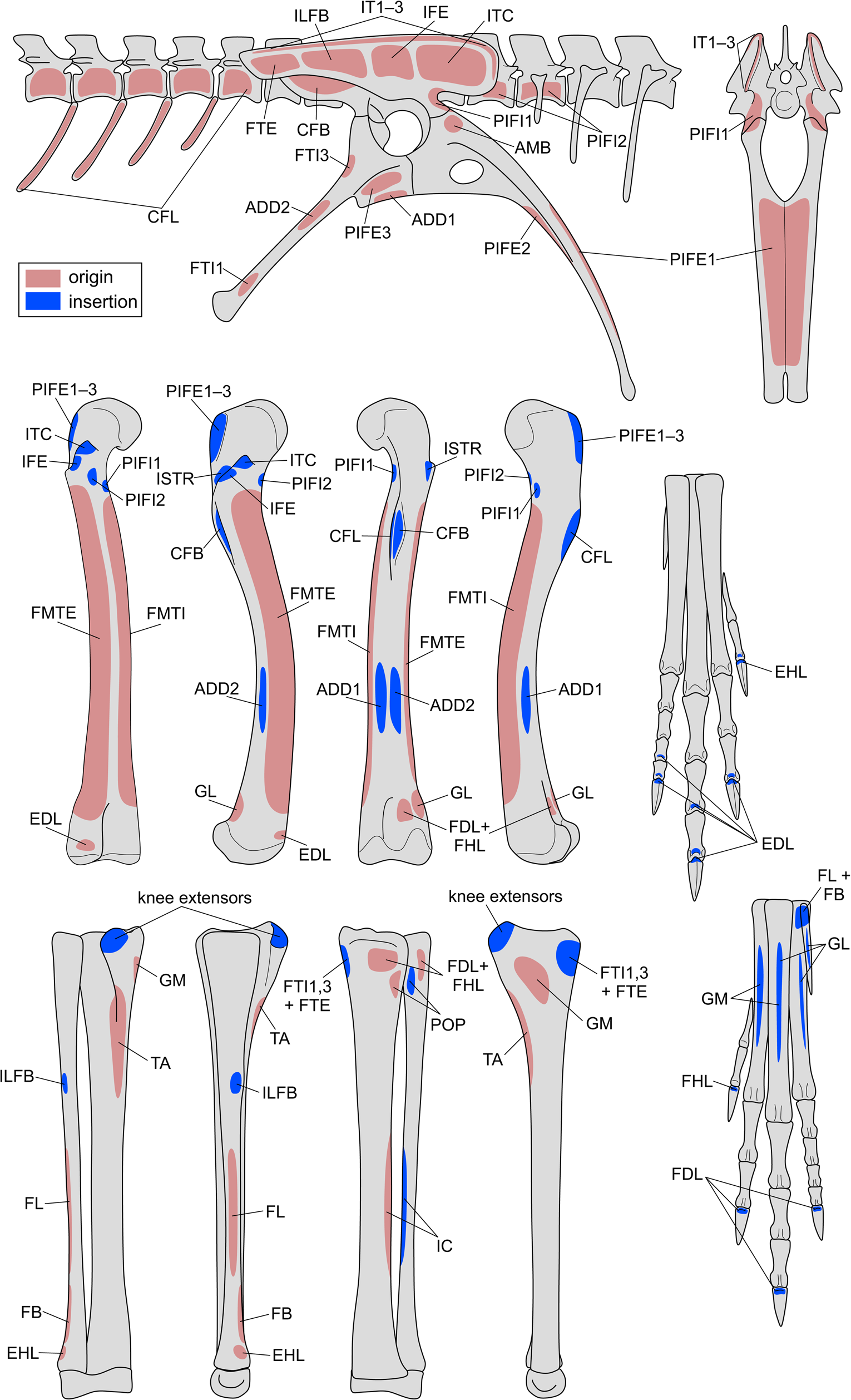
Reconstructed origins and insertions of hindlimb muscles in Coelophysis. Muscle abbreviations used in the musculoskeletal model are given in parentheses, and levels of inference (see also Witmer Reference Witmer and Thomason1995; Carrano and Hutchinson Reference Carrano and Hutchinson2002) are given in brackets. I = unambiguous with respect to the anatomy of extant taxa; II = ambiguous; III = inference unsupported by extant taxa; ′ = no osteological correlate present (weaker inference based on approximate position).

Developing Computational Musculoskeletal Models
Once a “muscle map” of origins and insertions has been derived for the anatomical system in question (Fig. 5), this reconstruction is transcribed to the articulated skeletal model to reconstruct the lines of action of muscle–tendon units (MTUs). A variety of proprietary software packages can be used to achieve this, including SIMM, AnyBody (AnyBody Technology A/S, Aalborg, Denmark), and MuJoCo (Roboti LLC, Redmond, Calif., U.S.A.), as well as the open-source OpenSim and GaitSym (Sellers Reference Sellers2016). Other geometric modeling software may be used, such as 3ds Max (Costa et al. Reference Costa, Rocha-Barbosa and Kellner2014), but whether the reconstructed MTU paths can be reliably used in downstream analyses remains to be verified. For example, there is cause for concern that the calculation of MTU moment arms may be problematic in nonbenchmarked software, especially when complex lines of action are involved (Sherman et al. Reference Sherman, Seth and Delp2013). Following Hicks et al. (Reference Hicks, Uchida, Seth, Rajagopal and Delp2015), we advocate the use of software that has been thoroughly documented and benchmarked in biomechanical applications.
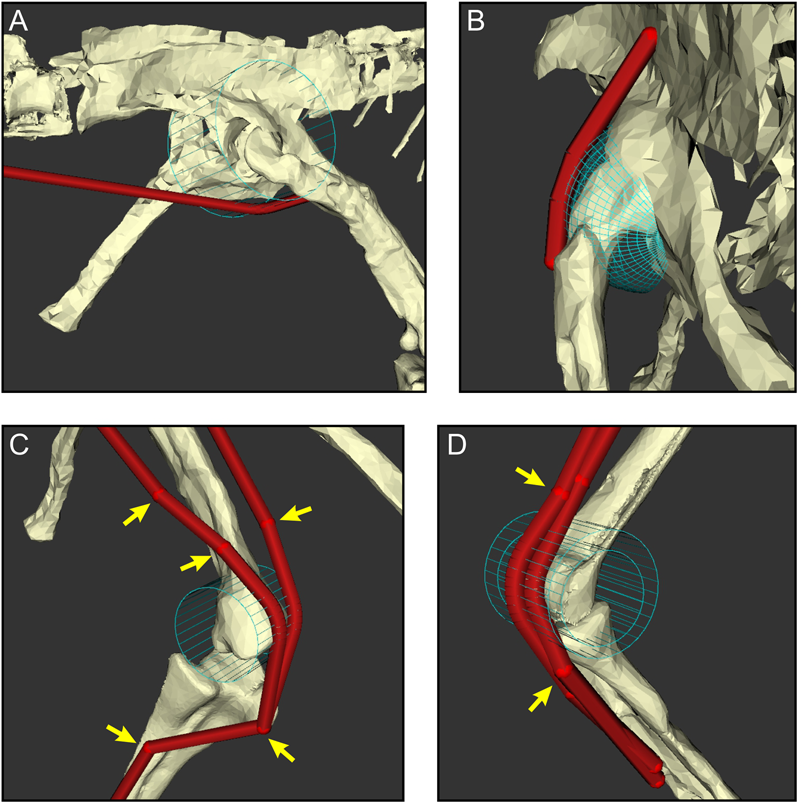
Here, MTU paths in OpenSim were created to run between the approximate centroids of origin and insertion. As in many previous studies of extinct archosaurs (Hutchinson et al. Reference Hutchinson, Anderson, Blemker and Delp2005, Reference Hutchinson, Miller, Fritsch, Hildebrandt, Endo and Frey2008; Bates and Schachner Reference Bates and Schachner2012; Bates et al. Reference Bates, Benson and Falkingham2012a,Reference Bates, Maidment, Allen and Barrettb; Brassey et al. Reference Brassey, Maidment and Barrett2017; Otero et al. Reference Otero, Allen, Pol and Hutchinson2017; Sellers et al. Reference Sellers, Pond, Brassey, Manning and Bates2017; Bishop et al. Reference Bishop, Hocknull, Clemente, Hutchinson, Farke, Barrett and Lloyd2018c; Bishop Reference Bishop2019), these paths were constrained to follow anatomically realistic lines of action across the full ROM of each joint, using a combination of “via points” and “wrapping surfaces.” Representative examples of these in the Coelophysis model are illustrated in Figure 6. Via points are points in space through which the MTU must pass, and wrapping surfaces are geometric primitives (available shapes in OpenSim are spheres, ellipsoids, cylinders, and tori) around which a given MTU is constrained to pass, following the shortest route to do so (Delp et al. Reference Delp, Loan, Hoy, Zajac, Topp and Rosen1990; Garner and Pandy Reference Garner and Pandy2000; Sherman et al. Reference Sherman, Seth and Delp2013). In OpenSim, while wrapping surfaces are fixed with respect to a given model segment, via points may be fixed or alternatively can be programmed to move as some a priori function of joint angle. This may be useful in studies involving extant species for which detailed information of muscle anatomy and behavior during limb movement can be ascertained (e.g., Hutchinson et al. Reference Hutchinson, Rankin, Rubenson, Rosenbluth, Siston and Delp2015; Rajagopal et al. Reference Rajagopal, Dembia, DeMers, Delp, Hicks and Delp2016; Cox et al. Reference Cox, Easton, Lear, Marsh, Delp and Rubenson2019), but we see this as introducing excessive assumptions into models of extinct species, and so here all via points were fixed. The disposition of via points and wrapping surfaces in the Coelophysis model was manually arranged based on our understanding of comparative anatomy in archosaurs, and only the minimal number of via points and wrapping surfaces needed to achieve this was used. Not only does this ensure that MTUs pass over joints in realistic ways, but it also prevents MTUs from passing through each other or bones, something that OpenSim cannot currently detect (but see Scholz et al. Reference Scholz, Sherman, Stavness, Delp and Kecskeméthy2015). In some prior studies (Hutchinson et al. Reference Hutchinson, Anderson, Blemker and Delp2005, Reference Hutchinson, Miller, Fritsch, Hildebrandt, Endo and Frey2008; Bates et al. Reference Bates, Benson and Falkingham2012a; Brassey et al. Reference Brassey, Maidment and Barrett2017; Bishop et al. Reference Bishop, Hocknull, Clemente, Hutchinson, Farke, Barrett and Lloyd2018c), muscles with expansive attachments have been modeled with multiple MTUs, effectively splitting up the muscle into subunits. This was followed here for two muscles whose origin on the iliac blade is inferred to have been sizable, the iliotibialis 2 (IT2) and iliotrochantericus caudalis (ITC), which were divided into anterior (a) and posterior (p) subunits. Additionally, although inferred to be present, some of the small distal muscles (e.g., popliteus, interosseous cruris) were not included in the musculoskeletal model, because they spanned the tibia and fibula; as these bones are fixed with respect to one another in the present study, the muscles involved have no functional relevance. In total, 33 MTUs were used for the hindlimb.
The judicious use of via points and wrapping surfaces can constrain muscle–tendon unit (MTU) paths to follow biologically realistic lines of action as they course from origin to insertion, shown here with examples of the right hindlimb. A, A wrapping cylinder used to guide the caudofemoralis longus around the hip. B, A wrapping sphere used to guide the iliofemoralis externus over the supra-acetabular crest and hip. C, A wrapping cylinder and via points (arrows) used to guide the iliotibialis 3 (left) and ambiens (right) over the knee. D, Via points and nested wrapping cylinders used to guide the gastrocnemius medialis (outer) and flexor hallucis longus (inner) around the ankle.
The process of creating MTU paths admittedly has considerable subjectivity, and error may creep in at multiple stages of path development. For instance, many muscles either do not have small, concentrated scars or lack direct evidence of attachment altogether, which hampers the precise locations of centroids of origin or insertion (Hutchinson et al. Reference Hutchinson, Anderson, Blemker and Delp2005; Brassey et al. Reference Brassey, Maidment and Barrett2017). Attachment centroids for these muscles must therefore be estimated, taking into account the anatomy of extant taxa and inferred relative positions of other muscles. A detailed explanation of the methodology used for the more problematic muscles in the Coelophysis model is presented in the Supplementary Material.
Sensitivity analysis of more uncertain aspects is an important component of the process here and can help ascertain how variations in model geometry, such as the placement and orientation of wrapping surfaces, may affect subsequent analyses (Hutchinson et al. Reference Hutchinson, Anderson, Blemker and Delp2005; Maidment et al. Reference Maidment, Bates, Barrett, Eberth and Evans2014a; Brassey et al. Reference Brassey, Maidment and Barrett2017). Yet even this may not be able to bring different models, developed by different research groups, to a level playing field for the purpose of comparison (Bates and Schachner Reference Bates and Schachner2012). Further discussion of the relative merits of different approaches to MTU path reconstruction, and the potential sensitivity of model results to these differences, is given by Brassey et al. (Reference Brassey, Maidment and Barrett2017), and also in the “Discussion.”
By itself, an articulated skeletal model with rigged MTU paths can be used to derive biomechanically relevant data in order to begin testing hypotheses. By far the most frequent approach in this regard has been the computation of muscle moment arms about specific joint axes; a moment arm (r) converts applied force (F) to joint moment (M) via the cross product
 $${\bf M} = {\bf r} \times {\bf F}.$$
The simplicity of this relationship means that, from a practical standpoint, it is quite straightforward to investigate questions of muscle action and leverage, how leverage may relate to posture and locomotor ability (Hutchinson et al. Reference Hutchinson, Anderson, Blemker and Delp2005; Bates et al. Reference Bates, Benson and Falkingham2012a), and how leverage differs across different morphologies (Bates and Schachner Reference Bates and Schachner2012; Maidment et al. Reference Maidment, Bates, Falkingham, VanBuren, Arbour and Barrett2014b). However, as noted previously (Hutchinson et al. Reference Hutchinson, Rankin, Rubenson, Rosenbluth, Siston and Delp2015; Brassey et al. Reference Brassey, Maidment and Barrett2017; Regnault and Pierce Reference Regnault and Pierce2018), there is much uncertainty surrounding what an individual muscle's moment arm (and how it varies with joint angle) actually means at the organismal level. At the very least, there is no demonstrated one-to-one correlation of moment arm magnitudes and the actual moment that a muscle can produce about a joint, let alone how this might relate to organismal locomotor abilities or performance. There are multiple reasons for this. First, a muscle-induced joint moment depends on both the moment arm and the applied force, the latter of which will vary nonlinearly with level of activation and the amount and rate of contraction or stretch of the muscle (Zajac Reference Zajac1989; Millard et al. Reference Millard, Uchida, Seth and Delp2013), which in turn vary with joint angle and angular velocity. The combined effect of this cascade of influences is that the joint angle at which muscle-induced moment is maximal is not necessarily the angle at which moment arm or muscle force is maximal (e.g., Lieber and Boakes Reference Lieber and Boakes1988). Moreover, muscles are frequently connected to bones via in-series tendons, and the compliance of these tendons can further modulate the force-producing capacity of the muscle (Millard et al. Reference Millard, Uchida, Seth and Delp2013; Cox et al. Reference Cox, Easton, Lear, Marsh, Delp and Rubenson2019). Muscles also rarely, if ever, act in isolation; they frequently act about a given joint with other muscles, and so it is the combined effect of multiple muscles (each of which may have differing moment arms, levels of activation, etc.) that produces the net joint moment that has greater relevance to locomotor behavior. This issue is further complicated by the effects of agonist–antagonist co-contraction (which is unknowable for fossil species) and muscle multi-articularity (Kuo Reference Kuo, Latash and Zatsiorsky2001; Valero-Cuevas Reference Valero-Cuevas2015). Measurements of moment arms in and of themselves have value for quantifying basic form–function relationships (e.g., muscle actions; Bates et al. Reference Bates, Maidment, Allen and Barrett2012b; Otero et al. Reference Otero, Allen, Pol and Hutchinson2017) and for generating hypotheses about muscle function or evolution, but there are more integrative ways that moment arms can be used in musculoskeletal modeling and simulation. We advocate a shift toward looking at the “bigger picture” of whole-limb function and performance (in the current context of locomotor biomechanics), which necessarily involves considering all muscles acting together as part of a single integrated entity. An example of how this could be done is given later on.
Reconstructing Muscle Physiology
As noted earlier, the moment-generating capacity of muscle depends in part on its force-generating capacity. Being able to estimate the maximal force different limb muscles could produce during locomotion would clearly progress biomechanical models toward increased realism. Although there are many other aspects of muscle physiology that could be explored (e.g., muscle force–velocity properties; including those informed by data from histochemistry in extant species), we focus here on maximal force production, as this is a key aspect in muscle function and is probably the most tractable to work with in extinct species. The maximal amount of force a muscle can produce during isometric contractions is related to its internal architecture by
 $$F_{\max } = \displaystyle{{m_{{\rm musc}}\cdot {\rm \sigma }\cdot \cos \,\lpar {\rm \alpha }_{\rm O}\rpar } \over {{\rm \rho }\cdot \ell _{\rm O}}}\comma \;$$
where m musc is muscle belly mass, σ is the maximum stress developed in the fibers, αo is pennation angle at optimum fiber length, ρ is muscle tissue density, and ℓ o is optimum fiber length. It should be noted that pennation angle is included in equation 2 only if muscle contraction is to be treated simply as a force along a line of action; if intrinsic force–length–velocity relationships are modeled (using a Hill-type model for instance), then pennation usually is not considered, as it is explicitly accounted for in the geometric underpinnings of these models (Zajac Reference Zajac1989; Cox et al. Reference Cox, Easton, Lear, Marsh, Delp and Rubenson2019). The parameters σ and ρ are generally taken to be constant for vertebrate skeletal muscle, around 300,000 N/m2 (Medler Reference Medler2002; Hutchinson Reference Hutchinson2004a; Bates and Falkingham Reference Bates and Falkingham2012; Sellers et al. Reference Sellers, Margetts, Coria and Manning2013; Hutchinson et al. Reference Hutchinson, Rankin, Rubenson, Rosenbluth, Siston and Delp2015) and 1060 kg/m3 (Mendez and Keys Reference Mendez and Keys1960; Hutchinson et al. Reference Hutchinson, Rankin, Rubenson, Rosenbluth, Siston and Delp2015), respectively. None of the other parameters are preserved in fossils, and so if they are to be estimated, this will need to be done via comparison to the anatomy of extant species. A previous approach to this task has been described by Sellers et al. (Reference Sellers, Margetts, Coria and Manning2013, Reference Sellers, Pond, Brassey, Manning and Bates2017). Briefly, muscle masses are estimated as a fixed proportion of body mass, taking into consideration each muscle's location in the limb and presumed gross function, and these are then converted to muscle volumes by a fixed value for density; fiber length is estimated from MTU lengths across the total range of possible limb movement (taking into account estimated ROM at each joint); then using equation 2 (ignoring pennation), F max is estimated. One caveat with this previous method that is of key relevance here is the estimation of relative muscle masses, which was based on data for a limited number (n = 3) of extant mammalian species.
We outline here an alternative procedure that may form a more useful foundation for studies of extinct archosaurs (Fig. 7). Using both published anatomical data for extant crocodylian and avian hindlimb muscles and new data derived from anatomical dissections, we have collated measurements of MTU length (L MTU), fiber length, muscle belly mass (m belly), and pennation angle for the main hindlimb muscles across a variety of species (Supplementary Table S2). For a given muscle or its homologue, a plot of normalized (size-independent) muscle mass and normalized fiber length was produced; the normalizations were computed as
 $$m{\rm \ast} = \displaystyle{{m_{{\rm muscle}}\times \;{\rm cos}\,\lpar {\rm \alpha }_{\rm O}\rpar } \over {m_{{\rm body}}}}\comma \;$$
 $$\ell {\rm \ast} = \displaystyle{{\ell _{\rm O}} \over {L_{{\rm MTU}}}}. $$
A novel method for estimating muscle fiber length and F max. A, Architectural data obtained from dissections of extant archosaurs include total muscle–tendon unit (MTU) length (L MTU), muscle belly mass (m belly), fiber length (ℓ o). and pennation angle (αo), as well as total body mass (m body). These are then used to produce normalized measures of muscle mass (m*) and fiber length (ℓ*), which are plotted against each other. B, Plot for the homologue of the femorotibialis internus (in crocodylians; femorotibiales intermedius et medialis in birds). C, Plot for the homologue of the flexor tibialis externus (in crocodylians, flexor cruris lateralis pars pelvica in birds). D, Plot for the extensor digitorum longus.
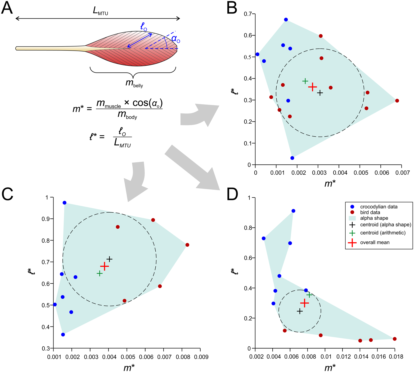
The incorporation of αo in equation 3 is for the sake of including an important architectural parameter that otherwise would be ignored when modeling muscles as forces along a line of action (as we do here). The normalization of ℓ o by L MTU in equation 4 stands in contrast to previous studies that have typically normalized by the cube root of body mass (Allen et al. Reference Allen, Elsey, Jones, Wright and Hutchinson2010; Bates and Schachner Reference Bates and Schachner2012; Dick and Clemente Reference Dick and Clemente2016); unlike these previous studies, the metric produced is truly dimensionless and also avoids the untestable assumption that fiber length scales with body mass in the same manner across all of Archosauria, which seems unlikely. Furthermore, in the context of locomotor biomechanics, fiber length would be expected to be more influenced by (and therefore correlated with) MTU or limb segment length than body mass (Hutchinson Reference Hutchinson2004a,Reference Hutchinsonb; Sellers et al. Reference Sellers, Margetts, Coria and Manning2013), especially considering the marked diversity in form and function (e.g., bipedal vs. quadrupedal postures) across Archosauria.
From the plotted values of m* and ℓ*, an “average” value of normalized mass and fiber length was derived, taken as the mean of (1) the arithmetic mean of the data and (2) the center of the largest circle able to be inscribed within an alpha shape fit to the data. The use of an alpha shape accommodates instances when the data are not evenly distributed across the plot (Fig. 7D gives one example), and this was performed using custom MATLAB code, provided in the Supplementary Material. The average values of normalized mass and fiber length may be seen as a “default guess” for a given archosaur, extinct or extant. Then, given body mass and MTU length for an extinct focal species (derived from models built in the steps outlined earlier), muscle-specific estimates of mass and fiber length, and in turn F max, are back-calculated. It should be noted that neither of the two methods covered here directly estimate muscle pennation, which in certain systems may have an important influence on system behavior (Zajac Reference Zajac1989; Bishop Reference Bishop2019) and could potentially be estimated by other means such as phylogenetic character mapping. Additionally, many animals possess muscles in which fiber pennation angle varies throughout a muscle belly, and hence a single value, as used in modeling, will not capture the (potentially important) internal heterogeneity in architecture (Dickinson et al. Reference Dickinson, Stark and Kupczik2018; Sullivan et al. Reference Sullivan, McGechie, Middleton and Holliday2019; Martin et al. Reference Martin, Travouillon, Fleming and Warburton2020). Other attendant caveats will be addressed in the “Discussion.”
Musculoskeletal Simulation and Hypothesis Testing
As with any modeling study, in vertebrate paleontology or any other aspect of science, the model that is developed and how it is used depends on the hypothesis to be tested (Anderson et al. Reference Anderson, Bright, Gill, Palmner and Rayfield2012; Hutchinson Reference Hutchinson2012; Hicks et al. Reference Hicks, Uchida, Seth, Rajagopal and Delp2015). Even within the realm of dinosaur locomotion studies, a wide diversity of models and methods have been used, and it is beyond the scope of the present work to review them all. Building upon our earlier remarks as well as prior studies (Hutchinson and Garcia Reference Hutchinson and Garcia2002; Hutchinson Reference Hutchinson2004a,Reference Hutchinsonb; Gatesy et al. Reference Gatesy, Bäker and Hutchinson2009), in this paper we emphasize understanding function and performance of the whole limb in locomotion, but uniquely by using musculoskeletal models of the complete limb. As an example, we focus on the single-stance phase of locomotion, asking the question “What is the maximal vertical ground reaction force that the hindlimb of Coelophysis was capable of withstanding?” The ground reaction force (GRF) is the force the feet experience from the ground as they push on it during the stance phase of locomotion (i.e., Newton's third law). As terrestrial vertebrates move faster, their feet tend to spend a smaller proportion of each stride cycle on the ground, which by conservation of momentum necessitates an increase in the vertical component of the GRF (Alexander et al. Reference Alexander, Maloiy, Njau and Jayes1979; Alexander and Jayes Reference Alexander and Jayes1980; Bishop et al. Reference Bishop, Graham, Lamas, Hutchinson, Rubenson, Hancock, Wilson, Hocknull, Barrett, Lloyd and Clemente2018a). Therefore, the ability to withstand higher GRFs may imply faster running ability (Weyand et al. Reference Weyand, Sternlight, Bellizzi and Wright2000). This fact has been used in several previous studies (Hutchinson and Garcia Reference Hutchinson and Garcia2002; Hutchinson Reference Hutchinson2004a,Reference Hutchinsonb; Gatesy et al. Reference Gatesy, Bäker and Hutchinson2009), which used simpler, 2D models to address maximal speed capabilities in various theropods by focusing on bulk moment balance at each joint. These previous studies used an “inverse simulation” technique, whereby a static limb posture (kinematics) and test GRF (kinetics) were inputs to the model, used to back-calculate muscular effort required to prevent limb collapse. This uses the same concepts employed in studies of dynamic behaviors of extant animals, such as human (Lin et al. Reference Lin, Dorn, Schache and Pandy2012; De Groote et al. Reference De Groote, Kinney, Rao and Fregly2016), rat (Johnson et al. Reference Johnson, Jindrich, Zhong, Roy and Edgerton2011), dog (Brown et al. Reference Brown, Bertocci, States, Levine, Levine and Howland2020), and emu walking (Goetz et al. Reference Goetz, Derrick, Pedersen, Robinson, Conzemius, Baer and Brown2008); ostrich running (Rankin et al. Reference Rankin, Rubenson and Hutchinson2016); horse galloping (Swanstrom et al. Reference Swanstrom, Zarucco, Hubbard, Stover and Hawkins2005); partridge wing flapping (Heers et al. Reference Heers, Rankin and Hutchinson2018); and sit-to-stand maneuvers in dogs (Ellis et al. Reference Ellis, Rankin and Hutchinson2018). An alternative to this is a “forward simulation” approach, using the model and a physics engine to directly generate dynamic gait cycles and produce kinematic and kinetic patterns de novo (Sellers and Manning Reference Sellers and Manning2007; Bates et al. Reference Bates, Manning, Margetts and Sellers2010; Sellers et al. Reference Sellers, Pond, Brassey, Manning and Bates2017). As this method involves explicit numerical integration of the system dynamic equations in generating a simulation, it can be extremely computationally expensive, which usually necessitates various modeling simplifications. For some behaviors or questions, the use of static versus dynamic and inverse versus forward analyses may not matter much (e.g., Anderson and Pandy Reference Anderson and Pandy2001; Lin et al. Reference Lin, Dorn, Schache and Pandy2012; Rankin et al. Reference Rankin, Rubenson and Hutchinson2016), but this deserves careful future scrutiny on a case-by-case basis.
Simulation
Using the Coelophysis model we have developed, complete with bones, joints, segment mass properties, and muscles, an inverse simulation in OpenSim was run to ascertain the maximum vertical GRF capable of being withstood. Additionally, we used the results obtained to test the hypothesis that in bipeds such as theropod dinosaurs, the ankle joint is the “weak link” that most constrains maximal running speed (Hutchinson Reference Hutchinson2004a,Reference Hutchinsonb). To investigate the effect of posture, three static, single-stance postures of the right leg were tested, spanning the continuum from upright to crouched, with the left leg in the same swing position each time (Fig. 8). The point of application of the GRF was consistently located approximately 40% of the way along digit III, near the center of the pes (Schaller et al. Reference Schaller, D'Août, Villa, Herkner and Aerts2011; Andrada et al. Reference Andrada, Rode and Blickhan2013b). In each posture, the stance limb was positioned so that the point of application of the GRF was located directly underneath the whole-body COM in the sagittal plane, and with digit III close to the body midline as would be expected for a fast-running theropod (Bishop et al. Reference Bishop, Clemente, Weems, Graham, Lamas, Hutchinson, Rubenson, Wilson, Hocknull, Barrett and Lloyd2017). A recursive technique with OpenSim's static optimization routine was used, whereby the magnitude of the GRF was set, and the optimizer solved for the combination of muscle activations am that would balance joint moments (i.e., achieve static equilibrium) while minimizing the sum of squared activations:
 $$\min \left({\sum\limits_{m = 1}^N {a_m^2 + \sum\limits_{q = 1}^Q {a_q^2 } } } \right)$$
 $${\rm subject}\;{\rm to}\quad \sum\limits_{i = 1}^n {F_i\cdot r_{i\comma k}} + M_{r\comma k} = M_k$$
 $${\rm and}\quad F_i = a_i\cdot F_{\max \comma i}\comma \;$$
for each degree of freedom k (= 6). There were N = 33 muscles and Q = 7 reserve actuators in the model, and the moment each muscle produced about a given degree of freedom was the product of its actual force Fi and its moment arm ri ,k. Additionally, muscle force was modeled as the product of activation and F max, ignoring intrinsic force–length–velocity relationships (eq. 7).
The three test postures used in the simulations, spanning from upright (A) to semi-crouched (B) to crouched (C). In each case the posture was configured so that the vertical ground reaction force (GRF; arrow) was directly underneath the whole-body center of mass (COM; checkered sphere) in the sagittal plane.

The magnitude of force was increased to the point that the routine could no longer find a solution to equation 6: the muscles were no longer able to withstand the applied load. Even though an exponent of 2 (i.e., muscle activation squared) was used here in computing the objective function, it is irrelevant in this context, as at maximal limb performance there is a unique solution, and therefore the formulation of the objective function is inconsequential; that is, the same result would be achieved using a different value for the exponent. Six “residual actuators” were applied at the COM of the body segment to actuate the joint between the body and the ground (global space), and infinitely strong reserve actuators (torque motors, Mr ,k) were appended to each degree of freedom in the left leg, obviating the need to solve for muscle activations in that limb (Hicks et al. Reference Hicks, Uchida, Seth, Rajagopal and Delp2015). As explained previously (Bishop et al. Reference Bishop, Hocknull, Clemente, Hutchinson, Barrett and Lloyd2018b,Reference Bishop, Hocknull, Clemente, Hutchinson, Farke, Barrett and Lloydc), a reserve actuator was also appended to the metatarsophalangeal joint of the right leg to accommodate likely insufficiencies in model strength at that joint. All degrees of freedom in the neck, tail, and forelimbs were locked in a standard position during simulation, equivalent to using infinitely strong reserve actuators. Once the simulation was set up, it only took a few minutes to reach a solution.
The technique used here is an advance on current state-of-the-art inverse analyses in at least three aspects. First, the model used was fully 3D. Second, individual muscles were used to balance joint moments, rather than abstracted “bulk muscle units” derived from estimates of total muscle volume and mean moment arm. Although our main goal here was to explore performance at the level of the whole limb, this approach nevertheless enables exploration of the contribution of individual muscles (see “Coelophysis Results”). The third improvement marked by the present approach is that, as vertical force was increased in the recursive routine, gravity was increased accordingly to produce net force balance (i.e., residual forces at the ground–body joint are zero). For instance, if the applied GRF is 2.5 times body weight (BW), then an acceleration of 2.5 × g (= 25.517 m/s2) is applied to all body segments. Previous studies used a constant gravitational acceleration of 1 × g, resulting in force disequilibrium in any applied GRF other than 1 BW.
Estimating muscle strength (F max) remains an outstanding issue in paleobiological enquiry (Bates and Falkingham Reference Bates and Falkingham2018), and this parameter is clearly important to the generation of high GRFs in running. Consequently, to explore the sensitivity of simulation results to how strength is estimated, we tested four variations in F max assignment for each MTU (Table 3), spanning different levels of complexity:
1. F max was constant for all MTUs, set to 2 BW (Bishop et al. Reference Bishop, Hocknull, Clemente, Hutchinson, Barrett and Lloyd2018b,Reference Bishop, Hocknull, Clemente, Hutchinson, Farke, Barrett and Lloydc).
2. F max was set according to which “functional group” a given MTU predominantly belonged to. As many MTUs crossed multiple joints and multiple degrees of freedom, there is no single way to objectively classify the functional group that a given MTU belonged to, but we followed a sensible first-pass classification. Moreover, for a given joint, the F max of flexor MTUs were set at half that of the corresponding extensor MTUs.
3. F max was set according to the proportions of body mass assigned by Sellers et al. (Reference Sellers, Pond, Brassey, Manning and Bates2017) for their model of Tyrannosaurus. In their model, muscle mass in each hindlimb comprised 22.5% of total body mass, but in our Coelophysis model the hindlimbs each comprised less than 10% of total body mass. As this <10% value ignored the mass in the sizable caudofemoralis longus (CFL; estimated at about 0.5 kg by Allen et al. Reference Allen, Bates, Li and Hutchinson2013), which resided almost wholly in the tail segment, we estimated that our Coelophysis had 11.25% of body mass as muscle mass in each hindlimb, that is, half of that in the Tyrannosaurus model. As noted earlier for the method of Sellers et al. (Reference Sellers, Pond, Brassey, Manning and Bates2017), fiber length is also required to estimate F max, which is computed as the change in length of the respective MTU across the limb's entire ROM. This was done with hip abduction and long-axis rotation set to 15° and 0°, respectively, and with the inferred long tendons of the ambiens (AMB) and fibularis longus (FL) trimmed from the MTU.
4. F max was set by following the novel data-driven method outlined earlier for estimating muscle mass and fiber length. The MTU lengths needed to estimate fiber length were measured from a “rest pose” in which hip abduction and long-axis rotation were set to 15° and 0°, respectively, and all other limb joints set approximately midway along their ROMs. The resulting estimated muscle masses (projected by pennation angle, as pennation is included in eq. 3) collectively totaled 1.18 kg, compared with a mass of the hindlimb in the model of 1.14 kg; as the mass of the CFL residing in the tail was ignored in the hindlimb mass, this discrepancy was considered plausible.
Values of muscle parameters for each muscle–tendon unit (MTU) in the four Coelophysis model variants tested. Muscle mass (m musc) is reported in grams (g), fiber length (ℓ o) is reported in meters (m), and F max is reported in multiples of body weight (BW); F max was estimated directly without recourse to architecture in variants 1 and 2. Also note that m musc for variant 4 is the muscle mass multiplied by the cosine of pennation angle. For muscle abbreviations, see Table 2. For “Muscle” column: 1 = hip flexors; 2 = hip extensors; 3 = knee extensors; 4 = hip abductors or rotators; 5 = knee flexors; 6 = ankle extensors; 7 = ankle flexors.
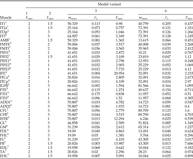
In all four F max variants, the reserve actuator appended to the metatarsophalangeal joint had a constant maximum output set equal to the product of BW and hip height in the neutral pose (64.04 Nm). The specific magnitude of this maximum output was not relevant, as long as it was sufficiently large to be recruited minimally in the optimization. Ultimately, a total of 12 combinations of posture and F max assignment were investigated.
Validation
To assess the realism of the simulation, we applied it to previously published musculoskeletal models of two extant obligate bipedal species, humans (Rajagopal et al. Reference Rajagopal, Dembia, DeMers, Delp, Hicks and Delp2016; mass = 75.3 kg) and ostriches (Rankin et al. Reference Rankin, Rubenson and Hutchinson2016; mass = 78.6 kg). Using kinematic data published with these models, a midstance running pose was derived and a vertical GRF was applied at the middle of the pes to provide the inputs for the simulation (Fig. 9A). In addition to the original muscle-specific values for F max, simulations were also run with all MTUs having F max set to a constant 2 BW, paralleling strength variant 1 of the Coelophysis model. Similar to the Coelophysis simulations, in the ostrich simulations a reserve actuator was appended to the metatarsophalangeal joint, of magnitude equal to the product of BW and hip height in the neutral pose (738 Nm). As humans are plantigrade, and therefore the ankle is the distalmost joint, no reserve actuator was used in the human model.
Results of the validation simulations for the human and ostrich models. A, Mid-stance running poses used in the simulations, with the location of the vertical ground reaction force (GRF; arrow) also shown. B, Maximum vertical GRF for the strength variants of both models; “original” refers to the model with muscle-specific values of F max as originally specified (Rajagopal et al. Reference Rajagopal, Dembia, DeMers, Delp, Hicks and Delp2016; Rankin et al. Reference Rankin, Rubenson and Hutchinson2016), and “2 BW” refers to the model where all muscle–tendon units (MTUs) had F max set at 2 BW (body weight). C, Mean level of activation across the extensor muscles of the hip, knee, and ankle joints for each model. See Supplementary Table S4 for the specific muscles used to compute each mean.

The maximum vertical GRF able to be attained for each model was between 2.5 and 3 BW (Fig. 9B); the muscle-specific model achieved higher force than the uniform 2 BW model in the human, but the result was reversed for the ostrich. Regardless, 2.5–3 BW is a modest underestimate of both species’ real capabilities. In fast running, non-athlete humans are able to generate peak vertical forces in excess of 3 BW at speeds of 6 m/s or more (Hamill et al. Reference Hamill, Bates, Knutzen and Sawhill1983; Nilsson and Thorstensson Reference Nilsson and Thorstensson1989; Keller et al. Reference Keller, Weisberger, Ray, Hasan, Shiavi and Spengler1996). While GRFs in fast running have not been measured for ostriches, using a previously published predictive model derived from empirical data for extant birds (including ostriches; Bishop et al. Reference Bishop, Graham, Lamas, Hutchinson, Rubenson, Hancock, Wilson, Hocknull, Barrett, Lloyd and Clemente2018a), the forces obtained for the ostrich model correspond to speeds of 7.1–10.8 m/s, lower than the fastest reliably recorded speed of >12 m/s (Alexander et al. Reference Alexander, Maloiy, Njau and Jayes1979; Daley et al. Reference Daley, Channon, Nolan and Hall2016). To explore muscle contributions to limb support, the mean level of activation across all extensor MTUs of the hip, knee, and ankle was calculated (Fig. 9C). In all simulations, the knee consistently had the highest level of recruitment (see also Supplementary Table S4), and therefore acted as the primary constraint on the limb's ability to withstand higher vertical GRFs, and in turn achieve faster running speeds.
Coelophysis Results
The maximum vertical GRF attained for each combination of posture and F max variant is reported in Figure 10A. The reserve actuator acting at the metatarsophalangeal joint was never recruited more than 17%, comparable to previous theropod simulation results (Bishop et al. Reference Bishop, Hocknull, Clemente, Hutchinson, Barrett and Lloyd2018b). Using the same published predictive model (Bishop et al. Reference Bishop, Graham, Lamas, Hutchinson, Rubenson, Hancock, Wilson, Hocknull, Barrett, Lloyd and Clemente2018a) and knowing the Coelophysis model's mass and limb length, maximal vertical GRF was also used to estimate the corresponding speed of locomotion (Fig. 10A). Knowing the hip height for each simulated posture, the faster speeds obtained here correspond to relative or dimensionless speeds (Alexander and Jayes Reference Alexander and Jayes1983) of 2.27–4.23. For comparison, the fastest known Triassic theropod trackway (made by an animal substantially larger than Coelophysis) displays a peak relative speed of 2.26 (Weems Reference Weems2006; Bishop et al. Reference Bishop, Clemente, Weems, Graham, Lamas, Hutchinson, Rubenson, Wilson, Hocknull, Barrett and Lloyd2017), although of course this does not necessarily indicate the maximal speed attainable by the trackmaker. Across all F max variants, more upright postures consistently allowed for higher GRFs to be sustained, consonant with principles derived from experimental studies of extant species (Biewener Reference Biewener1989, Reference Biewener1990; Gatesy and Biewener Reference Gatesy and Biewener1991). However, there was marked variation in the absolute magnitude of vertical GRF across the F max variants, ranging from 3.4 BW in the upright posture for variant 2 to less than 1 BW for the more crouched postures in variant 4. It should be noted that the two combinations for which maximal force was less than 1 BW are implausible, as this indicates that the model was not even able to support itself during standing on one leg and hence would be unable to walk. Interestingly, despite markedly different methods of F max assignment, the results from model variants 1 and 3 are very similar.
Results of the inverse simulations for Coelophysis. A, Maximum vertical ground reaction force (GRF) and corresponding speed of locomotion for each posture and F max variant. The two combinations marked with an apostrophe are implausible, as not even 1 BW (body weight) of GRF (dashed line) could be sustained; i.e., not even standing stationary on one leg was possible. B, Mean level of activation across the extensor muscles of the hip, knee, and ankle joints for each posture and F max variant. See Supplementary Table S5 for the specific muscles used to compute each mean.

Previously, Hutchinson (Reference Hutchinson2004b) examined vertical GRF resistance and running ability in Coelophysis, using a 2D posture most similar to posture 2 of the present study. This analysis was simpler in a number of respects, and the model used was distinctly more massive (20 kg) than the model used here. Hutchinson (Reference Hutchinson2004b) found that Coelophysis was easily able to withstand 2.5 BW of vertical force, whereas only one of the 12 variants in the present study was able to withstand a vertical GRF of that magnitude. The results obtained here therefore suggest lower maximal limb performance compared to previous estimates, although given the results of the validation test, these results should be interpreted as modest underestimates of true absolute performance capabilities in Coelophysis.
As for the human and ostrich simulations, the mean level of activation across all extensor MTUs of the hip, knee, and ankle was calculated for each Coelophysis simulation (Fig. 10B). Unlike the human and ostrich, however, it was the ankle that consistently had the highest level of recruitment across all postures and F max variants, and indeed most ankle extensors were maximally recruited (Supplementary Table S5). Therefore, in Coelophysis the ankle was the primary constraint on the limb's ability to withstand higher vertical GRFs in our simulations. The mixture of results obtained here casts doubt on the notion that the ankle is always the “weak link” in the limb of a biped, and invites future investigation to further tease apart how MTU anatomy and strength contribute to constraining limb performance.
A second noteworthy result here is that despite the vertical GRF passing anterior to the knee in the upright posture (Fig. 8A), all model variants were able to withstand it and arrive at a solution, meaning that the assumption of earlier studies (Hutchinson Reference Hutchinson2006; Hutchinson and Gatesy Reference Hutchinson and Gatesy2006; Gatesy et al. Reference Gatesy, Bäker and Hutchinson2009; Hutchinson and Allen Reference Hutchinson and Allen2009) that the GRF should pass posterior to the knee at midstance may not always be required (see also Andrada et al. Reference Andrada, Nyakatura, Bergmann and Blickhan2013a). This arises because the current model includes many multi-articular muscles (whereas previous studies used single-joint bulk muscles), which allows joints to influence one another as load is distributed along the limb. For instance, in helping to counteract ankle extension, the biarticular gastrocnemius lateralis also produces a flexor moment about the knee, partially counteracting the extension moment generated by the GRF and influencing the recruitment of other muscles spanning the knee, such as the femorotibiales (Supplementary Table S4). This reinforces the value of an integrative approach to modeling and simulation of musculoskeletal function.
Discussion
In this study we outlined a workflow for integrating paleontological data with biomechanical principles and modeling techniques, specifically in relation to understanding locomotion in nonavian dinosaurs. The structured process we have demonstrated with Coelophysis illustrates how each step of data collection and interpretation can feed into subsequent steps, and therefore clarifies what prerequisites are necessary for the answering of a particular research question. Although we often advocate certain aspects as what we believe to be best practice, we do not argue that the approach we have presented is “the” way to do it. Different researchers will use different methods of data collection, model development, and data analysis. This is often necessitated by historical and logistical constraints, data accessibility, software restrictions (particularly regarding proprietary software packages), and philosophical attitudes to different aspects of the workflow; many of these attitudes are rooted more in opinion than strict logic. Nevertheless, we do strongly encourage the use of an explicit, quantitative method, one that is rigorously grounded in physical principles and (where relevant) data from extant taxa. The data and computational capabilities now exist to enable stronger, more quantitative and more repeatable methodologies for testing paleobiological hypotheses.
Coelophysis and a New Modeling Workflow
In developing the Coelophysis model here, two key developments have been implemented upon prior studies, helping to improve rigor and transparency. First, an explicit geometry-based method of articulating digital bone models into a rigged skeletal marionette has been used, that takes bone (articular surface) geometries and objectively and deterministically results in a rigged skeleton. This is a technique long used in studies of extant taxa (Grood and Suntay Reference Grood and Suntay1983; Rubenson et al. Reference Rubenson, Lloyd, Besier, Heliams and Fournier2007; Li et al. Reference Li, Abram, Beaudoin, Berthiaume, Pelletier and Martel-Pelletier2008; Kambic et al. Reference Kambic, Roberts and Gatesy2014), but until now has yet to be applied to extinct taxa, and even in studies of extant taxa it is seldom automated. To help encourage the adoption of this approach, a set of MATLAB code for automatic fitting of geometric primitives has been provided in the Supplementary Material. Second, a whole-limb inverse approach to investigating locomotor function has been used in the musculoskeletal simulations. Again, the underlying method has long been used in studies of extant taxa (e.g., Swanstrom et al. Reference Swanstrom, Zarucco, Hubbard, Stover and Hawkins2005; Goetz et al. Reference Goetz, Derrick, Pedersen, Robinson, Conzemius, Baer and Brown2008; Johnson et al. Reference Johnson, Jindrich, Zhong, Roy and Edgerton2011; De Groote et al. Reference De Groote, Kinney, Rao and Fregly2016; Rankin et al. Reference Rankin, Rubenson and Hutchinson2016; Ellis et al. Reference Ellis, Rankin and Hutchinson2018; Heers et al. Reference Heers, Rankin and Hutchinson2018), and it has wide applicability to extinct taxa as well. The current inverse (and quasi-static) simulations were relatively rapid to perform, requiring only a few minutes per combination tested. If computing power is limiting, this method forms an attractive, if simplified, alternative to computationally intensive forward (and fully dynamic) simulations (Sellers and Manning Reference Sellers and Manning2007; Bates et al. Reference Bates, Manning, Margetts and Sellers2010; Sellers et al. Reference Sellers, Margetts, Coria and Manning2013, Reference Sellers, Pond, Brassey, Manning and Bates2017), or a useful step toward building a foundation for advancement of these methods.
Importantly, we also conducted similar simulations for a human and ostrich, obtaining results that were sufficiently close, as a first-pass estimate, to the known athletic performance of these species. This lends validity to the analysis and the simplifying assumptions that underpin it. However, we acknowledge that the “gold standard” test of validity—for the simulation step as well as all preceding steps—would have been to model these or other extant species as if their soft tissue anatomies were unknown, following the entire workflow outlined here using only the skeletal evidence that is available for extinct species. The simplified analyses of Hutchinson (Reference Hutchinson2004a) achieved such a result (to a degree) with various extant bipeds. Nevertheless, given that the validity of each step in the workflow outlined here has previously been examined in a variety of extant species (see relevant sections for citations of example studies), we suspect that the work-intensive procedure involved in achieving a “full” validation of the static simulations would likely not provide a manifestly stronger assessment of strengths and weaknesses than that already achieved here.
The results of the simulations undertaken here (Fig. 10) provide new perspective on locomotion in Coelophysis and nonavian theropods more generally. We infer that Coelophysis likely stood and moved with fairly extended limbs (upright posture), contrary to prior assessment that indicated the use of a substantially more flexed hip (Padian and Olsen Reference Padian, Olsen, Gillette and Lockley1989), but consistent with bone scaling and footprint data for nonavian theropods generally (Carrano Reference Carrano1998; Gatesy et al. Reference Gatesy, Middleton, Jenkins and Shubin1999; Hutchinson and Allen Reference Hutchinson and Allen2009). As also inferred in previous studies, the posture of Coelophysis and other early theropods was more upright than that of extant birds of comparable size, consistent with a gradual postural shift within Theropoda on the line to birds, in concert with various morphological transformations throughout the body (Hutchinson and Allen Reference Hutchinson and Allen2009; Allen et al. Reference Allen, Bates, Li and Hutchinson2013). Hindlimb joint morphology alone does not clarify the habitual posture of Coelophysis, because the joints have a large ROM (Fig. 3); rather, the biomechanics of musculoskeletal control dictate locomotor posture in real animals in vivo, including extinct species such as Coelophysis (principle of uniformitarianism). Our simulations therefore offer the best estimate yet of this animal's posture during fast running. That more upright postures improved locomotor performance in Coelophysis is consilient with studies of diverse extant species (Biewener Reference Biewener2005), although compared with previous modeling studies (Hutchinson Reference Hutchinson2004b; Gatesy et al. Reference Gatesy, Bäker and Hutchinson2009), absolute locomotor performance may have been lower than previously thought. The increased sophistication of a musculoskeletal model has further indicated that the ankle may well be a “weak link” in the hindlimbs of Coelophysis, but whether this is holds as a generality for all bipeds requires additional scrutiny.
As with all biomechanical studies in paleontology, the approach used with Coelophysis carries a number of important caveats. Those that have broader relevance to vertebrate paleontology as a whole will be explored in the following section. However, there are also a few caveats specific to the current study, particularly relating to the modeling and simulation aspects. Intrinsic force–length–velocity relationships of muscle were ignored in the simulations; even ignoring velocity effects as necessitated by a static analysis (as done here), the remaining effects of muscle optimal fiber length, pennation angle, and tendon compliance can interact to modulate force-generating capacity in important ways (Zajac Reference Zajac1989; Cox et al. Reference Cox, Easton, Lear, Marsh, Delp and Rubenson2019). Of greater immediate relevance, the results of sensitivity analysis of F max estimation demonstrated that inferences of locomotor performance are contingent on how muscle strength is determined. Although two variants (1 and 3) gave almost identical results, the other two gave widely diverging estimates of maximal sustainable vertical GRF. Perhaps surprisingly, variant 4, the most data-driven method (in terms of incorporating data from extant species) actually produced the least plausible results (Fig. 10A), as in two of the three postures tested the model was not even able to support itself during single-limb standing. The underlying issue here, which also affects the derivation of variant 3, is the estimation of individual muscle masses (m musc) and fiber lengths (ℓ o). Both are key determinants of F max (eq. 2) and previous sensitivity analyses have demonstrated their important effects on biomechanical inferences in extinct taxa (Hutchinson Reference Hutchinson2004b; Bates et al. Reference Bates, Manning, Margetts and Sellers2010; Bates and Falkingham Reference Bates and Falkingham2018; Bishop Reference Bishop2019). Variants 3 and 4 were derived on the basis (to one degree or another) of comparative data for extant species, but this does not account for the real possibility that extinct species such as nonavian theropods may have been structurally arranged in a markedly different fashion to any extant species: different sizes, shapes, proportions, postures, and (presumably) functions of the underlying skeleton may lead to muscle anatomy in an extinct species being adapted or “tuned” in ways that differ from those observed in any extant species (Bishop Reference Bishop2019).
We use the example of variant 4 to caution against the blind application of empirical anatomical datasets to a given extinct taxon, without first carefully considering if structural (e.g., skeletal) or functional differences necessitate transformation of empirically based values. Indeed, by analyzing all comparative architectural data together, the method used in variant 4 effectively treats any extinct archosaur as the same “everyarchosaur” (cf. Pagel Reference Pagel1991). A stronger approach would be to also take into consideration a given extinct taxon's morphological peculiarities (as variant 3 does to some extent) and phylogenetic position (cf. Fig. 7, Supplementary Table S1; note that crocodylians tend to have lower values of normalized mass), as well as biomechanical constraints or principles that are common to all terrestrial vertebrates. Thus, we argue that the best data-driven method to muscle architecture estimation is a “total evidence” one. To this end, further research on extant species (archosaur and non-archosaur) will help refine general principles relating muscular anatomy to function, such as how muscle attachment size and morphology correlate to architecture (Martin et al. Reference Martin, Travouillon, Sherratt, Fleming and Warburton2019; Fahn-Lai et al. Reference Fahn-Lai, Biewener and Pierce2020) or how long muscle fibers need to be to be able to effectively execute movement over a range of postures (Sellers et al. Reference Sellers, Margetts, Coria and Manning2013).
On a more minor note, the present simulations were static only. Although static and dynamic analyses can give comparable estimates of muscle activation patterns (Anderson and Pandy Reference Anderson and Pandy2001; Lin et al. Reference Lin, Dorn, Schache and Pandy2012), static analyses may underestimate absolute performance abilities. For example, static analyses ignore the potential for muscle force enhancement through active lengthening of fibers or stretch–shortening cycles during movement (Herzog Reference Herzog2014). More obviously, static simulations cannot be used to reconstruct gait cycles de novo for extinct species, although when used in an inverse sense could be used to test the feasibility of specific instances throughout a hypothetical gait cycle (Gatesy et al. Reference Gatesy, Bäker and Hutchinson2009).
Caveats, Assumptions, and Unknowns
There are also a number of broad caveats that will to some extent plague all biomechanical studies of extinct vertebrates. Most obviously, that only bones are usually preserved in the fossil record necessitates a variety of assumptions, simplifications, and sometimes tenuous analogies to extant taxa. Recently bemoaned in studies of joint range of motion, missing cartilage and other soft tissues (e.g., menisci) raise the question of how accurately the preserved joint shape reflects the “true,” in vivo joint shape, spacing, and articulation (Bonnan et al. Reference Bonnan, Sandrik, Nishiwaki, Wilhite, Elsey and Vittore2010, Reference Bonnan, Wilhite, Masters, Yates, Gardner and Aguiar2013; Lai et al. Reference Lai, Biewener and Pierce2018; Tsai et al. Reference Tsai, Turner, Manafzadeh and Gatesy2020; Demuth et al. Reference Demuth, Rayfield and Hutchinson2020). Articular cartilage also raises concern over the use of objective shape-fitting algorithms in the determination of anatomical and joint coordinate systems, as done here: Does the absence of cartilage lead to a markedly different skeletal marionette? Quantitative anatomical studies of extant taxa are needed to address this concern. Related to the topic of coordinate system generation, taphonomic distortion of bones will also affect the process, either through direct modification of articular surface geometries (Brassey et al. Reference Brassey, Maidment and Barrett2017) or through modifying the spatial relationships of proximal and distal ends of the same bone, such as through twisting or bending of the intervening diaphysis.
As alluded to earlier, musculoskeletal modeling in particular encounters a plethora of unknowns, even in just the generation of MTU lines of action. In addition to difficulty in precisely locating the centroid of origin or insertion for certain muscles (particularly those with broad, fleshy attachments), recreating the lines of action around joints is problematic. This is due to both subjectivity in the creation of how MTUs wrap around a joint (e.g., the use of just via points, or with wrapping surfaces, and if so, which ones, and what are their sizes and locations?), and the unknown influence that adjacent soft tissues such as fat deposits, bursae, and other muscles could have. Recently, a few studies of extant species have used various digital anatomical techniques to more objectively recreate MTU lines of action (contrast-enhanced computed tomography [Allen et al. Reference Allen, Kambic, Gatesy and Hutchinson2017]; probe digitization [Hutchinson et al. Reference Hutchinson, Rankin, Rubenson, Rosenbluth, Siston and Delp2015; Cox et al. Reference Cox, Easton, Lear, Marsh, Delp and Rubenson2019]; magnetic resonance imaging [Modenese and Kohout Reference Modenese and Kohout2020]). We are in the process of using contrast-enhanced computed tomography to develop more accurate models of birds and crocodylians, and it may be possible to one day apply the results of those studies to models of extinct archosaurs.
There is also limited current understanding of how muscle anatomy in extant species relates to their underlying skeletal anatomy, the only direct evidence available for extinct species (Bryant and Seymour Reference Bryant and Seymour1990). It was noted earlier how both m musc and ℓ o are crucial for better modeling muscle function, and therefore the more accurate determination of their values in extinct taxa represents a key challenge for future work. For instance, the study of how m musc relates to actual attachment area, type of osteological correlate, and muscle identity may reveal relationships that can be used to produce more anatomically grounded estimates in extinct taxa (Martin et al. Reference Martin, Travouillon, Sherratt, Fleming and Warburton2019; Fahn-Lai et al. Reference Fahn-Lai, Biewener and Pierce2020). Similarly, the accurate estimation of ℓ o poses another key challenge. In both variants 3 and 4 of the Coelophysis model investigated here, ℓ o was based, at least in part, from a measure of MTU length in the musculoskeletal model. The derivation of variant 3 hinges on the assumption that ℓ o should be such that fibers experience ±50% length change across joint ROM (Sellers and Manning Reference Sellers and Manning2007; Sellers et al. Reference Sellers, Margetts, Coria and Manning2013, Reference Sellers, Pond, Brassey, Manning and Bates2017), which although based on the principles of Hill-type models of muscle contraction (Zajac Reference Zajac1989), nevertheless remains untested for a range of behaviors in extant taxa. The derivation of variant 4 sets ℓ o in proportion to MTU length, which can lead to unconventional and widely disparate estimates of F max for muscles within the same homologous group that have disparate MTU lengths (Table 3). For example, F max of the CFL is 34% of that of the CFB, whereas the large tail and relatively early-diverging phylogenetic position of Coelophysis would suggest that this taxon had a very sizable CFL, which was much stronger than the CFB (Gatesy Reference Gatesy1990). Building upon our earlier suggestion, future work could therefore incorporate additional information specific to the anatomy of Coelophysis to better guide estimation of F max, such as considering the size of attachment areas for the CFL on the tail (cf. Hutchinson et al. Reference Hutchinson, Bates, Molnar, Allen and Makovicky2011; Allen et al. Reference Allen, Bates, Li and Hutchinson2013) and the CFB on the brevis fossa of the ilium.
Other aspects of muscle control that rarely receive attention in paleobiological studies include the components of physiology that extend beyond gross architecture, such as histochemical differences (slow vs. fast fibers, and associated activation–deactivation dynamics) and neuromuscular control. Moreover, modeling a whole muscle with a single MTU, typically employing some form of Hill-type model of contraction (e.g., Millard et al. Reference Millard, Uchida, Seth and Delp2013), essentially reduces the muscle down to a single fiber. This simplification of homogeneity is frequently questioned in extant animal biomechanical studies (Ahn et al. Reference Ahn, Monti and Biewener2003; Carr et al. Reference Carr, Ellerby and Marsh2011a,Reference Carr, Ellerby, Rubenson and Marshb; Winters et al. Reference Winters, Takahashi, Lieber and Ward2011; Infantolino et al. Reference Infantolino, Neuberger and Challis2012). Often the default assumption in many of these aspects is one of gross phyletic conservatism (McMahon Reference McMahon1984; Zajac Reference Zajac1989), but the experimental data underlying these models are typically based on a limited sample of muscles and species (although see Medler Reference Medler2002; Rospars and Meyer-Vernet Reference Rospars and Meyer-Vernet2016).
One final unknown concerning musculoskeletal control involves structures that passively exert forces and moments (e.g., ligaments, joint capsules, bony stops), which probably provide an important contribution to joint control during certain tasks, particularly when joints are near a limit to ROM about a given axis. Inverse musculoskeletal simulations of locomotion and other behaviors in extant species have frequently found that muscle forces alone cannot produce observed movement and force patterns, requiring the use of reserve actuators or the like to account for joint moment deficits (Hicks et al. Reference Hicks, Uchida, Seth, Rajagopal and Delp2015; Rankin et al. Reference Rankin, Rubenson and Hutchinson2016; Charles et al. Reference Charles, Cappellari and Hutchinson2018; Ellis et al. Reference Ellis, Rankin and Hutchinson2018; Heers et al. Reference Heers, Rankin and Hutchinson2018). In the Coelophysis simulations undertaken, a reserve actuator was only used at the metatarsophalangeal joint, principally to account for incomplete knowledge of musculature crossing that joint (Bishop et al. Reference Bishop, Hocknull, Clemente, Hutchinson, Barrett and Lloyd2018b); in reality, passive contributions to joint moment balance were likely possible at all joints in the limb, although not necessarily in the postures tested for here.
Moving Forward
In this study we have taken broad philosophical and methodological perspectives on how to address biomechanical questions in extinct vertebrates, building on prior views (e.g., Alexander Reference Alexander1991; Anderson et al. Reference Anderson, Bright, Gill, Palmner and Rayfield2012; Hutchinson Reference Hutchinson2012) to promote a balanced, pragmatic approach. In doing so, we have offered recommendations on “best practice” and identified specific areas for future improvement, similar to Hicks et al. (Reference Hicks, Uchida, Seth, Rajagopal and Delp2015) for human studies. There are aspects of the methods that are more subjective (e.g., mass property estimation, musculoskeletal reconstruction) and some that are more objective (e.g., estimation of joint axes, biomechanical analysis), but we suggest that even the more subjective end of the spectrum is valuable progress when studies are transparent about the methods and underlying evidence used. The more uncertain or subjective input data or methods nonetheless require more validation and sensitivity analysis (Hutchinson Reference Hutchinson2012). Even for techniques that have been previously validated against one or more extant species in the past, we argue that validation is never “done”: successive studies that use these techniques should conduct additional, critical validation that is appropriate to the specific research question or taxon involved. As noted earlier, we have not undertaken all possible aspects of validation that could be done in this study (e.g., simulating humans and ostriches with estimated rather than observed soft tissue morphology inputs). Nevertheless, that our results for Coelophysis are broadly consilient with the findings of previous studies provides a form of retrospective validation, perhaps better termed “consensus building” (Bates and Falkingham Reference Bates and Falkingham2018). This also increases confidence that the workflow has merit for analysis of other (more contentious or enigmatic) taxa in future and can form the basis for more sophisticated simulations than conducted here.
One view that is sometimes encountered in biomechanical analyses of extinct species is that of pessimism or cynicism to varying degrees: biomechanical analyses of extinct taxa are too subjective, speculative, or assumption-laden to be feasible, or even taken seriously scientifically. The opposite philosophical vantage point, one of naïve optimism, can also exist. The quantitative precision and rigor offered by biomechanical methods may give the illusion that the results obtained are somehow “better” (Alexander Reference Alexander1991), leading to advancements without necessary checking of assumptions or model sensitivity, especially if the results obtained seem plausible (Hicks et al. Reference Hicks, Uchida, Seth, Rajagopal and Delp2015). We contend that both extremes in attitude are biases that can impede progress. As simplified representations of a complex reality, all models are by definition “wrong.” However, sometimes “getting it wrong” as well as “getting it right” can cumulatively help to create net progress over time. For instance, where a model fails to replicate reality may sometimes highlight a previously underappreciated aspect of the system that deserves future study; one present example is the apparent diversity in which particular joints may act as the principal limit on force resistance in a biped (ankle in Coelophysis, knee in humans and ostriches). One additional benefit of biomechanical models in particular is that by relating different aspects of a system together in a precise and mechanistic fashion, it is easier to understand how different sources of uncertainty will affect higher-level inferences (Witmer Reference Witmer and Thomason1995; Bates and Falkingham Reference Bates and Falkingham2018). We encourage a skeptical and cautious perspective to the uncertainties involved in working with fossil data, navigating between extreme pessimism and optimism. Integrated with all available lines of evidence, including phylogenetic and geologic data, this facilitates the exploration of how muscle, bone, and joint function, as well as whole-organism performance and adaptation, contributed to ecological interactions and lineage diversification (or extinction) through deep time.
Acknowledgments
We thank the “DAWNDINOS” team of V. Allen, K. Michel, A. Wiseman, L. Kermode, R. Pintore, and O. Demuth for their input on this paper, and likewise to other past and present members of J.R.H.'s broader team, including E. Herbst, J. Rankin, and V. La Barbera. We have benefited from innumerable insights and helpful discussions over many years with many people, which have helped shape our own views on aspects presented here, as well as in this broader area of research; in alphabetical order they are M. Alexander, R. Barrett, K. Bates, C. Clemente, M. Daley, F. De Groote, S. Delp, A. Falisse, B. Full, S. Gatesy, D. Henderson, S. Hocknull, R. Kambic, T. Keaveny, R. Kram, D. Lloyd, A. Manafzadeh, C. McHenry, K. Padian, M. Phillips, C. Richards, H. Richards, J. Rubenson, and M. Turner. Comments from S. Gatesy, A. Manafzadeh, O. Demuth, and two anonymous reviewers on earlier drafts of the article are greatly appreciated. This paper is based on a presentation delivered by J.R.H. at the Ninth International Symposium on Adaptive Motion of Animals and Machines, and the organizers of that symposium are thanked for the invitation to present the work contained here, which stimulated the writing of the paper. The research was supported by an ERC Horizon 2020 Advanced Investigator Grant (695517, to J.R.H.).
All authors helped conceive the study design; A.R.C. and J.R.H. produced digital models; all authors collected anatomical data; P.J.B. developed MATLAB code and carried out simulations; all authors contributed to results interpretation and writing the article; all authors approved the final draft.


 Open access