


1. Introduction
Moonpools refer to vertical openings in drillships or offshore construction vessels, and are prone to resonance problems due to external wave excitation and wave-induced motion of the floating structures. It is crucial to predict the natural frequencies, which include the piston mode and sloshing modes, the latter being similar to the sloshing in the tanks of liquefied natural gas (LNG) ships. Several studies have been conducted to predict the natural frequencies of two- and three-dimensional moonpools without a recess (Molin Reference Molin2001; Molin et al. Reference Molin, Zhang, Huang and Remy2018; Tan et al. Reference Tan, Lu, Tang, Cheng and Chen2019). Additionally, it is important to predict and analyse the free-surface response inside moonpools, which can be studied through numerical simulations or model tests in wave tanks (Tan et al. Reference Tan, Lu, Tang, Cheng and Chen2019; Xu et al. Reference Xu, Zhang, Chu and Huang2020).
Some new moonpool designs in drillships feature ‘recesses’, which are sub-compartments used for assembling subsea equipment (Son et al. Reference Son, Choi, Kim and Hwangbo2008). Molin (Reference Molin2017) proposed a theoretical model to compute the natural frequencies of moonpools in drillships with a recess using the eigenfunction expansion method. In that model, the flow inside the moonpool is assumed to be two-dimensional, allowing for the consideration of a piston mode and longitudinal sloshing modes. Newman (Reference Newman2018) proposed a method using Legendre polynomials to evaluate the natural modes in moonpools with recesses. Specifically, a simplified model was developed to estimate the sloshing frequency based on the standing-wave approximation. Later, Zhang & Li (Reference Zhang and Li2021) extended this method to study the sloshing problem in three-dimensional rectangular moonpools with recesses on two sides.
On the other hand, nonlinear responses inside moonpools are also important, as their amplitudes can be much larger than those of the linear responses. Ravinthrakumar et al. (Reference Ravinthrakumar, Kristiansen, Molin and Ommani2020) conducted experiments in a wave basin to investigate the impact of moonpool responses on vessel motions and secondary resonances for three different moonpools without recesses. Zhao et al. (Reference Zhao, Wolgamot, Taylor and Taylor2017) studied nonlinear gap resonance through experiments in a wave basin and identified various harmonics using the phase separation method. Chu, Zhang & Zhang (Reference Chu, Zhang and Zhang2022) computed the nonlinear response inside a two-dimensional moonpool with a recess using a fully nonlinear two-dimensional boundary element method based on the mixed Euler–Lagrange scheme. Their model also included a pressure drop component to account for viscous-induced damping effects. Song et al. (Reference Song, Lu, Tang, Lou and Liu2023) investigated the nonlinear piston-mode responses in a gap formed between two ships using a fully nonlinear potential flow model. The higher-harmonic components of the free-surface elevation in the narrow gap can also be analysed using a two-dimensional numerical wave tank based on computational fluid dynamics (CFD), where viscous damping effects are inherently taken into account (Gao et al. Reference Gao, Chen, Zang, Chen, Wang and Zhu2020; Jiang, Bai & Yan Reference Jiang, Bai and Yan2021; Ding et al. Reference Ding, Walther and Shao2022a , Reference Ding, Walther and Shaob ). However, the computational cost of using CFD is considerably higher compared with potential flow-based solvers.
It is worth noting that most previous studies on nonlinear moonpool responses have focused on configurations without recesses. Introducing a recess not only changes the effective size of the moonpool but also modifies the water depth in the fluid domain above the recess, thereby influencing the free-surface response inside the moonpool. Ravinthrakumar et al. (Reference Ravinthrakumar, Kristiansen, Molin and Ommani2019) investigated a two-dimensional moonpool with a recess, examining the linear response and damping effects through extensive wave-flume experiments. However, the nonlinear free-surface behaviour within three-dimensional moonpools featuring recesses remains poorly understood, and the influence of recesses on such nonlinear responses is still an open question. Moreover, it is crucial to develop an efficient model for estimating the natural frequencies and modes of a three-dimensional moonpool with a recess, taking into account sloshing behaviour in the longitudinal, transverse and diagonal directions.
In the present study, we address the piston and sloshing modes within a relevant range of wave periods for a ship in typical sea conditions, aiming to understand how these modes affect the moonpool responses. A ship model incorporating four distinct moonpool configurations, each characterised by different recess lengths, was systematically examined through model tests conducted in the Deepwater Wave Basin at Shanghai Jiao Tong University. The findings underscore the critical role of the secondary resonance induced by super-harmonics, as well as the associated nonlinear hydrodynamic responses.
The ultimate goal is to understand moonpool responses under realistic sea conditions with the ship in free motion, and to explore the coupled dynamics between the moonpool and the drillship. However, it is essential to first examine the behaviour with the ship fixed before proceeding to scenarios where the ship is freely floating.
The rest of this paper is organised as follows. Section 2 introduces the domain decomposition method used to compute the natural frequencies of three-dimensional moonpools with recesses. The experimental set-up and conditions are described in § 3. Section 4 presents the validation of the theoretical model, analyses experimental results including regular wave tests, white-noise tests, NewWave-type focused wave group tests and provides discussions. Finally, the conclusions are summarised in § 5.
2. Domain-decomposition method
A domain-decomposition method is developed to determine the natural frequencies of the resonant modes in a recessed, three-dimensional moonpool of a ship in deep water. This method builds upon the approach introduced in Molin (Reference Molin2017), which considered moonpools with a three-dimensional flow field outside and a two-dimensional flow inside. In contrast, the model proposed in this study incorporates three-dimensional flow within the moonpool, allowing for the analysis of both transverse and longitudinal sloshing modes. A detailed explanation of this method is provided in Appendix A.
3. Experimental set-up
The experiments were carried out in the Deepwater Wave Basin at Shanghai Jiao Tong University. This wave basin measures 50 m in length, 40 m in width and has an adjustable water depth ranging from 0 to 10 m using an artificial bottom. For these experiments, the depth was set to 5 m. According to the wave dispersion relation, all test cases qualify as deep water scenarios. Flap-hinged wavemakers are installed along two adjacent sides of the basin, while wave-absorbing beaches are positioned on the opposite sides to minimise wave reflections from the basin boundaries.
As shown in figure 1, a ship with a recessed moonpool (RMP) was used in the experiments. The coordinate system is also indicated, with its origin at the moonpool centre. Four representative configurations are included in the experiments. For comparison purposes, one configuration with a moonpool without a recess (also called ‘clean’ moonpool) and three configurations with RMPs were considered and tested in the wave basin. The moonpool is 80 cm long and 40 cm wide. The height of recess, $h_r$
, is 10 cm. Three different recess lengths,
$h_r$
, is 10 cm. Three different recess lengths, $l_r$
, of 20 , 30 and 40 cm, are tested, and the corresponding RMPs are denoted as RMP2, RMP3 and RMP4, respectively. Table 1 provides a summary of all regular wave test cases and their key parameters. In the regular wave cases, most have a steepness of
$l_r$
, of 20 , 30 and 40 cm, are tested, and the corresponding RMPs are denoted as RMP2, RMP3 and RMP4, respectively. Table 1 provides a summary of all regular wave test cases and their key parameters. In the regular wave cases, most have a steepness of $\epsilon =H/ \lambda =1/80$
, with some cases at
$\epsilon =H/ \lambda =1/80$
, with some cases at $\epsilon =1/160$
to examine the effect of wave steepness. Here, the wave height
$\epsilon =1/160$
to examine the effect of wave steepness. Here, the wave height $H$
(crest-to-trough value) is twice the wave amplitude
$H$
(crest-to-trough value) is twice the wave amplitude $A$
, and
$A$
, and $\lambda$
represents the wavelength.
$\lambda$
represents the wavelength.
Diagram of a drillship featuring a RMP in an ocean wave basin subjected to head waves. ( $a$
) Top view; (
$a$
) Top view; ( $b$
) side view. The dimensions of the ship model are as follows: length (bow to stern)
$b$
) side view. The dimensions of the ship model are as follows: length (bow to stern) $L=$
4 m, width
$L=$
4 m, width $B=$
0.8 m, draught
$B=$
0.8 m, draught $d=$
0.3 m. The moonpool dimensions are
$d=$
0.3 m. The moonpool dimensions are $l=$
0.8 m in length and
$l=$
0.8 m in length and $b=$
0.4 m in width. The length and height of the recess are indicated by
$b=$
0.4 m in width. The length and height of the recess are indicated by $l_r$
and
$l_r$
and $h_r$
, respectively, with
$h_r$
, respectively, with $h_r$
being fixed at 0.1 m. In the
$h_r$
being fixed at 0.1 m. In the $x$
–
$x$
– $y$
plane (plan view), the coordinates of WG1–WG5 are (0.39 m, −0.19 m), (0.2 m, −0.19 m), (0, −0.19 m), (−0.2 m, −0.19 m) and (−0.39 m, −0.19 m), respectively. WG6–WG10 are symmetric to WG1–WG5 about the centreline (the
$y$
plane (plan view), the coordinates of WG1–WG5 are (0.39 m, −0.19 m), (0.2 m, −0.19 m), (0, −0.19 m), (−0.2 m, −0.19 m) and (−0.39 m, −0.19 m), respectively. WG6–WG10 are symmetric to WG1–WG5 about the centreline (the $x$
-axis) of the ship.
$x$
-axis) of the ship.

Main parameters of test cases in regular waves. Here, $l_r$
denotes the recess length and
$l_r$
denotes the recess length and $A$
is the regular wave amplitude.
$A$
is the regular wave amplitude.
 $^*$
This represents the cases with a small wave steepness of
$^*$
This represents the cases with a small wave steepness of $\epsilon =1/160$
, along with the more commonly considered condition of
$\epsilon =1/160$
, along with the more commonly considered condition of $\epsilon =1/80$
.
$\epsilon =1/80$
.
For RMP0, incident wave periods are selected near the piston-mode period (approximately 1.4 s) and at half the first longitudinal frequency $\omega _{10}$
to investigate super-harmonic secondary resonance, defined by
$\omega _{10}$
to investigate super-harmonic secondary resonance, defined by $n \omega =\omega _{pq}$
(
$n \omega =\omega _{pq}$
( $n\geqslant 2$
and
$n\geqslant 2$
and $p+q\geqslant 1$
), where
$p+q\geqslant 1$
), where $n$
denotes the super-harmonic order,
$n$
denotes the super-harmonic order, $\omega$
is the excitation frequency, and
$\omega$
is the excitation frequency, and $p$
and
$p$
and $q$
are the longitudinal and transverse mode numbers, respectively. Here,
$q$
are the longitudinal and transverse mode numbers, respectively. Here, $\omega _{pq}$
represents the sloshing frequency of the three-dimensional moonpool. The same strategy is repeated for RMP2–RMP4 to select test cases, using their respective piston-mode periods of 1.65, 1.85 and 2.1 s.
$\omega _{pq}$
represents the sloshing frequency of the three-dimensional moonpool. The same strategy is repeated for RMP2–RMP4 to select test cases, using their respective piston-mode periods of 1.65, 1.85 and 2.1 s.
In the test cases for RMP4, we also include off-resonance points, such as the wave period of 1.45 s, to investigate the potential response in the first sloshing mode although the actual response depends on the bandwidth of the first sloshing mode. Additionally, 1.8 and 1.9 s are considered to assess the response under near-resonance conditions. As summarised in the table, the wave steepness for three cases (2.1, 2.15 and 2.2 s) is set to 1/160, since the responses at these periods are very large and can even reach the deck at a steepness of 1/80. Therefore, additional cases with reduced wave steepness were tested. Moreover, a case with a wave period of 2.3 s and a steepness of 1/80 is included to study the effect of the off-secondary frequency.
The experimental models are 1 : 40 scaled versions of generalised yet realistic vessels. The ship was rigidly mounted on a gantry (blue) in the central area of the wave basin. The gantry provided sufficient stiffness to prevent vibrations of the ship model. The moonpool centre was located 25 m away from the wave paddles and 20 m from the sidewalls of the wave basin. A snapshot of the ship model, showing both the gantry and the ship, is presented in figure 2.
A snapshot of the ship model (yellow) with a moonpool rigidly connected to the gantry (blue).

Both regular wave tests and white-noise irregular wave tests were conducted. In the white-noise irregular wave tests, the lower and upper cut-off frequencies were $\omega _l = 1.5 $
and
$\omega _l = 1.5 $
and $\omega _u = 11 \ \text{rad}\,\text{s}^{-1}$
, respectively. The target significant wave height was
$\omega _u = 11 \ \text{rad}\,\text{s}^{-1}$
, respectively. The target significant wave height was $H_s = 40 \ \text{mm}$
. The irregular waves consisted of time series of 20 min. Satisfactory agreement was found between the target and measured wave spectra in the Wave Basin, with the significant wave height
$H_s = 40 \ \text{mm}$
. The irregular waves consisted of time series of 20 min. Satisfactory agreement was found between the target and measured wave spectra in the Wave Basin, with the significant wave height $H_s$
differing by only 1 %. In addition, NewWave focused wave group tests were performed to examine nonlinear effects due to different harmonics. Ten wave gauges (WG1 to WG10) were placed inside the moonpool to measure the free-surface elevations with five WGs on each side, with a couple of other WGs placed around the ship model (see figure 1).
$H_s$
differing by only 1 %. In addition, NewWave focused wave group tests were performed to examine nonlinear effects due to different harmonics. Ten wave gauges (WG1 to WG10) were placed inside the moonpool to measure the free-surface elevations with five WGs on each side, with a couple of other WGs placed around the ship model (see figure 1).
In a random sea with a power spectral density $S(\omega )$
, the shape of a unidirectional NewWave group is given by
$S(\omega )$
, the shape of a unidirectional NewWave group is given by
 \begin{eqnarray} \eta (x,t)=\frac {\alpha }{\sigma ^2} \sum _{n=1}^{N} S(\omega _n)\triangle \omega \mathrm{Re}(\mathrm{e}^{-\mathrm{i} k_n(x-x_0)+ \mathrm{i} \omega _n (t-t_0)+\mathrm{i} \psi }), \end{eqnarray}
where $\eta (x,t)$
is the free-surface profile of the focused wave group of NewWave type. Here,
$\eta (x,t)$
is the free-surface profile of the focused wave group of NewWave type. Here, $\alpha$
corresponds to the expected maximum free-surface elevation in a given sea state,
$\alpha$
corresponds to the expected maximum free-surface elevation in a given sea state, $N$
is the number of wave components,
$N$
is the number of wave components, $\psi$
is the phase angle and
$\psi$
is the phase angle and $k_n$
and
$k_n$
and $\omega _n$
are the wavenumber and frequency of each wave component, respectively, with the variance
$\omega _n$
are the wavenumber and frequency of each wave component, respectively, with the variance $\sigma ^2=\sum _{n=1}^{N} S(\omega _n)\triangle \omega$
.
$\sigma ^2=\sum _{n=1}^{N} S(\omega _n)\triangle \omega$
.
In the present study, the NewWave (NW) group is generated using a Gaussian spectrum (American Bureau of Shipping 2016)
 \begin{eqnarray} S(\omega )=\frac {H_s^2}{16} \frac {1}{\sqrt {2\pi \delta ^2}}\exp \left (-\frac {(\omega -\omega _p)^2}{2\delta ^2}\right ). \end{eqnarray}
The spectrum parameters are provided in table 2. The largest wave crest occurs at the focusing position and time $(x_0, t_0)$
with phase angle
$(x_0, t_0)$
with phase angle $\psi =0$
. For each NW ‘set’ in table 2, four NW groups were generated using the same paddle signal, with each component phase shifted by
$\psi =0$
. For each NW ‘set’ in table 2, four NW groups were generated using the same paddle signal, with each component phase shifted by ${0}^{\circ }$
,
${0}^{\circ }$
, ${90}^{\circ }$
,
${90}^{\circ }$
, ${180}^{\circ }$
or
${180}^{\circ }$
or ${270}^{\circ }$
. The linear component and the nonlinear harmonics of both the incident wave and the response are extracted using a linear combination of the four-phase time histories. After using the Stokes-type expansion of the surface elevation written here up to the twelfth order in the linear component amplitude
${270}^{\circ }$
. The linear component and the nonlinear harmonics of both the incident wave and the response are extracted using a linear combination of the four-phase time histories. After using the Stokes-type expansion of the surface elevation written here up to the twelfth order in the linear component amplitude $A$
, the four-phase harmonic extraction can be summarised as follows:
$A$
, the four-phase harmonic extraction can be summarised as follows:
 \begin{align} \frac {\zeta _0-\zeta _{90}^H-\zeta _{180}+\zeta _{270}^H}{4}&=\left (Aa_{1,1}+A^3a_{3,1}+A^5a_{5,1}+A^7a_{7,1}+A^9a_{9,1}+A^{11}a_{11,1}\right )\cos \theta \nonumber \\ &\quad+\left (A^5a_{5,5}+A^7a_{7,5}+A^9a_{9,5}+A^{11} a_{11,5}\right )\cos 5\theta \nonumber \\ &\quad+(A^9a_{9,9}+A^{11} a_{11,9})\cos 9\theta +O(A^{13}),\\[-11pt]\nonumber \end{align}
 \begin{align} \frac {\zeta _0-\zeta _{90}+\zeta _{180}-\zeta _{270}}{4}&=\left (A^2a_{2,2}+A^4a_{4,2}+A^6a_{6,2}+A^8a_{8,2}+A^{10}a_{10,2}+A^{12}a_{12,2}\right ) \nonumber \\ &\quad\times\cos 2\theta+\left (A^6a_{6,6}+A^8a_{8,6}+A^{10}a_{10,6}+A^{12}a_{12,6} \right )\cos 6\theta \nonumber \\ &\quad+(A^{10}a_{10,10}+A^{12}a_{12,10}) \cos 10\theta +O(A^{14}),\\[-11pt]\nonumber \end{align}
 \begin{align} \frac {\zeta _0+\zeta _{90}^H-\zeta _{180}-\zeta _{270}^H}{4}&=\left (A^3a_{3,3}+A^5a_{5,3}+A^7a_{7,3}+A^9a_{9,3}+A^{11} a_{11,3}\right )\cos 3\theta \nonumber \\ &\quad+(A^7a_{7,7}+A^9 a_{9,7}+A^{11} a_{11,7})\cos 7\theta \nonumber \\ &\quad+ A^{11} a_{11,11}\cos 11\theta +O(A^{13}),\\[-11pt]\nonumber \end{align}
 \begin{align} \frac {\zeta _0+\zeta _{90}+\zeta _{180}+\zeta _{270}}{4}&=A^2a_{2,0}+A^4a_{4,0}+A^6a_{6,0}+A^8a_{8,0}+A^{10}a_{10,0}+A^{12}a_{12,0}\nonumber \\ &\quad+\left (A^4a_{4,4}+A^6a_{6,4}+A^8a_{8,4}+A^{10}a_{10,4}+A^{12}a_{12,4}\right )\cos 4\theta \nonumber \\ &\quad+ (A^8a_{8, 8}+A^{10} a_{10, 8}+A^{12} a_{12, 8})\cos 8\theta \nonumber \\ &\quad+ A^{12} a_{12, 12}\cos 12\theta +O(A^{14}),\\[-11pt]\nonumber \end{align}
where $\zeta$
represents the time history of the free-surface response inside the moonpool, superscript
$\zeta$
represents the time history of the free-surface response inside the moonpool, superscript $H$
denotes the Hilbert transforms and the subscripts correspond to the shifted four phases of the signals. Here,
$H$
denotes the Hilbert transforms and the subscripts correspond to the shifted four phases of the signals. Here, $a_{i,j}$
are the coefficients in the expansion. By employing a twelfth-order expansion of the free-surface elevations, responses containing up to the twelfth harmonic can be determined.
$a_{i,j}$
are the coefficients in the expansion. By employing a twelfth-order expansion of the free-surface elevations, responses containing up to the twelfth harmonic can be determined.
Parameters of test cases using NW-type wave groups. Here, $T_p$
is the peak period of the spectrum adopted for the generation of the transient wave group. The relation between the peak frequency and peak period is
$T_p$
is the peak period of the spectrum adopted for the generation of the transient wave group. The relation between the peak frequency and peak period is $\omega _p=2\pi /T_p$
. Also,
$\omega _p=2\pi /T_p$
. Also, $\delta$
is the shape parameter of the spectrum related to the bandwidth and
$\delta$
is the shape parameter of the spectrum related to the bandwidth and $\alpha$
is the maximum surface elevation.
$\alpha$
is the maximum surface elevation. $k_p$
is the wavenumber corresponding to peak period.
$k_p$
is the wavenumber corresponding to peak period.

It is important to note that this method relies on the assumption that weakly nonlinear wave–wave and wave–structure interactions can be described using a Stokes-type expansion of the surface elevation. The validity of this separation method for the present problem will be addressed in a subsequent section.
4. Results and discussion
4.1. Natural periods and modal shapes
4.1.1. Natural periods and modal shapes
The natural modes and modal shapes obtained by solving the eigenvalue problem are compared with the experimental measurements under white-noise irregular waves and calculations using the diffraction code WAMIT. By analysing the response time series of the WGs inside the moonpool using the fast Fourier transform, we can obtain the response spectra. The frequencies corresponding to the peaks in the response spectra are the natural frequencies of the piston and sloshing modes. Then, by using the response amplitude at different WGs at natural frequencies, we can obtain the natural modes.
Natural frequencies of one moonpool without recess (RMP0) and three moonpools with a recess of different lengths (RMP2, RMP3, RMP4). The experimental data from white-noise irregular wave tests are compared with the predictions using the theoretical model described in Appendix A and the diffraction/radiation code WAMIT. Here, $(m, n)$
refers to the mode combined with longitudinal and transverse directions (similar definition in Molin et al. (Reference Molin, Zhang, Huang and Remy2018)).
$(m, n)$
refers to the mode combined with longitudinal and transverse directions (similar definition in Molin et al. (Reference Molin, Zhang, Huang and Remy2018)).
 $^*$
12.41122106
$^*$
12.41122106 $^\dagger$
12.41123132.
$^\dagger$
12.41123132.
The natural frequencies are summarised in table 3. In the table, the $(m, n)$
values represent the dominant geometric modes
$(m, n)$
values represent the dominant geometric modes $(\cos mx \cos ny)$
in the modal shapes of the free-surface elevation. For example, mode 1 with
$(\cos mx \cos ny)$
in the modal shapes of the free-surface elevation. For example, mode 1 with $m=n=0$
is the piston mode. Mode 2 with
$m=n=0$
is the piston mode. Mode 2 with $m=1$
and
$m=1$
and $n=0$
is the first sloshing mode in the longitudinal direction for all four moonpool configurations. Mode 3 with
$n=0$
is the first sloshing mode in the longitudinal direction for all four moonpool configurations. Mode 3 with $m=2$
and
$m=2$
and $n=0$
is the second sloshing mode in the longitudinal direction for RMP0. However, for RMP2, RMP3 and RMP4, mode 3 is the first transverse sloshing mode (
$n=0$
is the second sloshing mode in the longitudinal direction for RMP0. However, for RMP2, RMP3 and RMP4, mode 3 is the first transverse sloshing mode ( $m=0$
and
$m=0$
and $n=1$
) as its frequency is slightly lower than that of the second sloshing mode in the longitudinal direction. This can be attributed to the fact that the recess affects the sloshing mode frequencies. As shown in the table, for all four moonpools, mode 7 with
$n=1$
) as its frequency is slightly lower than that of the second sloshing mode in the longitudinal direction. This can be attributed to the fact that the recess affects the sloshing mode frequencies. As shown in the table, for all four moonpools, mode 7 with $m=3$
and
$m=3$
and $n=0$
is the third sloshing mode in the longitudinal direction.
$n=0$
is the third sloshing mode in the longitudinal direction.
As shown in the table, for the four moonpool configurations, the theoretical predictions of the natural frequencies for the first three resonant modes are in good agreement with both the white-noise irregular wave test results and the WAMIT computations. This consistency is particularly evident for the first three longitudinal sloshing modes, i.e. $m=1$
,
$m=1$
, $m=2$
and
$m=2$
and $m=3$
with
$m=3$
with $n=0$
. It should be noted that not all sloshing modes can be excited in the white-noise irregular wave tests, since each wave component has a small steepness and the signal bandwidth is limited. Consequently, only the piston mode and the first three sloshing modes can be identified from these tests.
$n=0$
. It should be noted that not all sloshing modes can be excited in the white-noise irregular wave tests, since each wave component has a small steepness and the signal bandwidth is limited. Consequently, only the piston mode and the first three sloshing modes can be identified from these tests.
The comparisons of the modal shapes for the four moonpools are illustrated in figure 3. Generally, the modal shapes obtained from the present theoretical model agree well with the experimental measurements and WAMIT results, although there is a small difference in the piston mode for RMP0. This discrepancy can be attributed to the effect of wave heading, which is not accounted for in the theoretical model proposed in this study. Note that the heading effect is relatively minor for the sloshing modes. For the piston mode in cases with recesses, a slight discrepancy is observed between the eigenvalue solution and the experimental data from the white-noise irregular wave tests; however, this difference decreases as the recess length increases. For the first sloshing mode, as shown in panels ( $a\,\textrm{i}$
) to (
$a\,\textrm{i}$
) to ( $d\,\textrm{i}$
), the predicted modal shapes agree quite well with the experimental measurements in all moonpool configurations. As illustrated in panels (
$d\,\textrm{i}$
), the predicted modal shapes agree quite well with the experimental measurements in all moonpool configurations. As illustrated in panels ( $a\,\textrm{ii}$
) to (
$a\,\textrm{ii}$
) to ( $d\,\textrm{ii}$
) in figure 3, the difference in the modal shape of the second sloshing mode becomes a little more pronounced as the recess length increases. This can be attributed to the damping effect caused by flow separation around the sharp recess corner, which influences the maximum free-surface elevation occurring near the midsection of the moonpool (i.e. at
$d\,\textrm{ii}$
) in figure 3, the difference in the modal shape of the second sloshing mode becomes a little more pronounced as the recess length increases. This can be attributed to the damping effect caused by flow separation around the sharp recess corner, which influences the maximum free-surface elevation occurring near the midsection of the moonpool (i.e. at $x=0$
) at the second sloshing mode.
$x=0$
) at the second sloshing mode.
Modal shapes of the piston, first and second sloshing modes (longitudinal direction) for four moonpools with different recess lengths. The subplots of each column correspond to the modal shapes of RMP0, RMP2, RMP3 and RMP4, respectively. Here, $\zeta _R$
denotes the maximum wave elevation above the recess. The number on the right side of each panel index denotes the resonance type, where ‘0’ refers to the piston mode and ‘i’ and ‘ii’ correspond to the first sloshing and the second sloshing modes in the longitudinal direction, respectively. The labels ‘
$\zeta _R$
denotes the maximum wave elevation above the recess. The number on the right side of each panel index denotes the resonance type, where ‘0’ refers to the piston mode and ‘i’ and ‘ii’ correspond to the first sloshing and the second sloshing modes in the longitudinal direction, respectively. The labels ‘ $a$
’, ‘
$a$
’, ‘ $b$
’, ‘
$b$
’, ‘ $c$
’ and ‘
$c$
’ and ‘ $d$
’ refer to the cases for RMP0, RMP2, RMP3 and RMP4, respectively.
$d$
’ refer to the cases for RMP0, RMP2, RMP3 and RMP4, respectively.

Moreover, as presented in table 3, it is interesting to note the presence of modes 9 and 10 for RMP0, which are not the true double mode or quadruple mode. Their natural frequencies, while differing by only $10^{-5}$
, are not identical. They both have geometric modes (4, 0) and (0, 2) that contribute with different signs. This observation aligns with the findings in Molin et al. (Reference Molin, Zhang, Huang and Remy2018), suggesting that the connection of the moonpool domain with the lower fluid domain creates a coupling between the geometric modes. However, this phenomenon is not observed for RMP2, RMP3 and RMP4, possibly due to the influence of the recess.
$10^{-5}$
, are not identical. They both have geometric modes (4, 0) and (0, 2) that contribute with different signs. This observation aligns with the findings in Molin et al. (Reference Molin, Zhang, Huang and Remy2018), suggesting that the connection of the moonpool domain with the lower fluid domain creates a coupling between the geometric modes. However, this phenomenon is not observed for RMP2, RMP3 and RMP4, possibly due to the influence of the recess.
4.2. Piston-mode resonance and secondary resonance due to super-harmonics
Through analysing the experimental data around the piston-mode frequencies, we obtained the response amplitudes of different harmonics using short-time fast Fourier transform (STFT). Figure 4 shows the typical time series of the surface elevation measured at WG1, along with the corresponding amplitude spectra. In the plots on the left, the time on the horizontal axis is non-dimensionalised by the incoming wave period $T$
. The base frequency for the four test cases, corresponding to the four panels in the figure, is nearly the same, with
$T$
. The base frequency for the four test cases, corresponding to the four panels in the figure, is nearly the same, with $T \approx 2$
s and a circular frequency
$T \approx 2$
s and a circular frequency $\omega \approx 3.14$
rad s–1 (see the parameters in table 1).
$\omega \approx 3.14$
rad s–1 (see the parameters in table 1).
Time histories and amplitude spectra of the surface elevation at WG1 near secondary resonances for the first longitudinal sloshing mode are presented for four different moonpools. Panels ( $a\,\textrm{i}$
) and (
$a\,\textrm{i}$
) and ( $a\,\textrm{ii}$
) show RMP0, wave period
$a\,\textrm{ii}$
) show RMP0, wave period $T=1.95$
s; (
$T=1.95$
s; ( $b\,\textrm{i}$
) and (
$b\,\textrm{i}$
) and ( $b\,\textrm{ii}$
) show RMP2, wave period
$b\,\textrm{ii}$
) show RMP2, wave period $T=2.1$
s; (
$T=2.1$
s; ( $c\,\textrm{i}$
) and (
$c\,\textrm{i}$
) and ( $c\,\textrm{ii}$
) show RMP3, wave period
$c\,\textrm{ii}$
) show RMP3, wave period $T=2.1$
s; (
$T=2.1$
s; ( $d\,\textrm{i}$
) and (
$d\,\textrm{i}$
) and ( $d\,\textrm{ii}$
) show RMP4, wave period
$d\,\textrm{ii}$
) show RMP4, wave period $T=2.05$
s. Here,
$T=2.05$
s. Here, $A$
is the incident wave amplitude, and wave steepness
$A$
is the incident wave amplitude, and wave steepness $\epsilon =1/80$
. The time series between the two red vertical dashed lines are used to evaluate the amplitude spectra.
$\epsilon =1/80$
. The time series between the two red vertical dashed lines are used to evaluate the amplitude spectra.

Higher harmonics are observed to amplify significantly as the recess length increases. This phenomenon can be attributed to the slight reduction in the first sloshing mode frequency, $\omega _{10}$
, as the recess length
$\omega _{10}$
, as the recess length $l$
increases to 40 cm (see table 3). As a result, the double-frequency components at
$l$
increases to 40 cm (see table 3). As a result, the double-frequency components at $2\omega$
approach the first sloshing mode frequency,
$2\omega$
approach the first sloshing mode frequency, $\omega _{10}$
, in the longitudinal direction. Furthermore, as the recess length increases, the resonance amplitude of the piston mode also rises, as will be shown later in this paper. This behaviour is similar to that observed in a two-dimensional moonpool with a recess (Tan et al. Reference Tan, Lu, Tang, Cheng and Chen2019), and leads to the generation of additional resonant second-harmonic components. Figure 5 shows the results measured at WG5, whose tendency is similar to that for WG1. The only difference is that, for RMP3 and RMP4, the higher harmonics at WG5 exceed the first harmonics. This is because the first harmonic, also known as the linear component, is weaker at WG5 compared with WG1 (placed above the recess). This behaviour is also evident in the modal shapes illustrated in figure 3. Additionally, by comparing the results shown in figures 4 and 5, it is evident that nonlinear effects are more pronounced in the region above the recess.
$\omega _{10}$
, in the longitudinal direction. Furthermore, as the recess length increases, the resonance amplitude of the piston mode also rises, as will be shown later in this paper. This behaviour is similar to that observed in a two-dimensional moonpool with a recess (Tan et al. Reference Tan, Lu, Tang, Cheng and Chen2019), and leads to the generation of additional resonant second-harmonic components. Figure 5 shows the results measured at WG5, whose tendency is similar to that for WG1. The only difference is that, for RMP3 and RMP4, the higher harmonics at WG5 exceed the first harmonics. This is because the first harmonic, also known as the linear component, is weaker at WG5 compared with WG1 (placed above the recess). This behaviour is also evident in the modal shapes illustrated in figure 3. Additionally, by comparing the results shown in figures 4 and 5, it is evident that nonlinear effects are more pronounced in the region above the recess.
Time histories and amplitude spectra of the free-surface elevation at WG5 near secondary resonances for the first longitudinal sloshing mode. Four different moonpools are considered. Panels ( $a\,\textrm{i}$
) and (
$a\,\textrm{i}$
) and ( $a\,\textrm{ii}$
) show RMP0, wave period
$a\,\textrm{ii}$
) show RMP0, wave period $T=1.95$
s; (
$T=1.95$
s; ( $b\,\textrm{i}$
) and (
$b\,\textrm{i}$
) and ( $b\,\textrm{ii}$
) show RMP2,
$b\,\textrm{ii}$
) show RMP2, $T=2.1$
s; (
$T=2.1$
s; ( $c\,\textrm{i}$
) and (
$c\,\textrm{i}$
) and ( $c\,\textrm{ii}$
) show RMP3,
$c\,\textrm{ii}$
) show RMP3, $T=2.1$
s; (
$T=2.1$
s; ( $d\,\textrm{i}$
) and (
$d\,\textrm{i}$
) and ( $d\,\textrm{ii}$
) show RMP4,
$d\,\textrm{ii}$
) show RMP4, $T=2.05$
s. Here,
$T=2.05$
s. Here, $A$
is the incident wave amplitude, wave steepness
$A$
is the incident wave amplitude, wave steepness $\epsilon =1/80$
. The time series between the two red vertical dashed lines are used to evaluate the amplitude spectra, as the incident wave has reached a steady state.
$\epsilon =1/80$
. The time series between the two red vertical dashed lines are used to evaluate the amplitude spectra, as the incident wave has reached a steady state.

Figures 6 to 9 present the results for all cases across different moonpool configurations. The primary wave steepness is $\epsilon = 1/80$
, with additional cases of
$\epsilon = 1/80$
, with additional cases of $\epsilon = 1/160$
included for RMP3 and RMP4. The higher harmonics, up to the fourth order, are extracted, with the natural frequencies of the piston and different sloshing modes indicated. In these figures,
$\epsilon = 1/160$
included for RMP3 and RMP4. The higher harmonics, up to the fourth order, are extracted, with the natural frequencies of the piston and different sloshing modes indicated. In these figures, $\zeta _n(\omega '=n\omega )$
denotes the amplitude of the nth harmonic, obtained from the STFT and defined as follows:
$\zeta _n(\omega '=n\omega )$
denotes the amplitude of the nth harmonic, obtained from the STFT and defined as follows:
 \begin{eqnarray} \zeta (\boldsymbol{x},t)=\sum _{n=1}^{N} \zeta _n (\boldsymbol{x}) \mathrm{Re}(\mathrm{e}^{\mathrm{i} n\omega t+\mathrm{i}\psi _n}), \end{eqnarray}
where $\zeta _n(\boldsymbol{x})$
denotes the amplitude of the
$\zeta _n(\boldsymbol{x})$
denotes the amplitude of the $n{\text{th}}$
harmonic component of the free-surface elevation,
$n{\text{th}}$
harmonic component of the free-surface elevation, $\boldsymbol{x}=(x, y)$
denotes the position vector,
$\boldsymbol{x}=(x, y)$
denotes the position vector, $\psi _n$
is the corresponding phase angle and
$\psi _n$
is the corresponding phase angle and $N$
is the total number of harmonics considered.
$N$
is the total number of harmonics considered.
Variation of the first four harmonic amplitudes of free-surface elevations with frequency at various locations inside RMP0. Regular head waves are considered, with a wave steepness of $\epsilon =1/80$
. Panels show (
$\epsilon =1/80$
. Panels show ( $a$
) WG1; (
$a$
) WG1; ( $b$
) WG3; (
$b$
) WG3; ( $c$
) WG5; (
$c$
) WG5; ( $d$
) WG6; (
$d$
) WG6; ( $e$
) WG8; (
$e$
) WG8; ( $f$
) WG10. Here,
$f$
) WG10. Here, $\omega _{mn}$
, marked by dashed vertical black lines, denotes the natural frequencies predicted by the proposed theoretical model for dominant
$\omega _{mn}$
, marked by dashed vertical black lines, denotes the natural frequencies predicted by the proposed theoretical model for dominant $(m,n)$
(see table 3) and
$(m,n)$
(see table 3) and $A$
is the incident regular wave amplitude.
$A$
is the incident regular wave amplitude.

Variation of the first four harmonic amplitudes of free-surface elevations with frequency at various locations inside RMP2 with a recess length of $l_r=20$
cm. Regular head waves are considered, with a wave steepness of
$l_r=20$
cm. Regular head waves are considered, with a wave steepness of $\epsilon =1/80$
. Panels show (
$\epsilon =1/80$
. Panels show ( $a$
) WG1; (
$a$
) WG1; ( $b$
) WG3; (
$b$
) WG3; ( $c$
) WG5; (
$c$
) WG5; ( $d$
) WG6; (
$d$
) WG6; ( $e$
) WG8; (
$e$
) WG8; ( $f$
) WG10.
$f$
) WG10.

Variation of the first four free-surface-elevation harmonic amplitudes with frequency at various locations inside RMP3 with a recess length of $l_r=30$
cm. Regular head waves are considered, with a primary wave steepness of
$l_r=30$
cm. Regular head waves are considered, with a primary wave steepness of $\epsilon = 1/80$
and supplementary cases of
$\epsilon = 1/80$
and supplementary cases of $\epsilon = 1/160$
(green triangles). Panels show (
$\epsilon = 1/160$
(green triangles). Panels show ( $a$
) WG1; (
$a$
) WG1; ( $b$
) WG3; (
$b$
) WG3; ( $c$
) WG5; (
$c$
) WG5; ( $d$
) WG6; (
$d$
) WG6; ( $e$
) WG8; (
$e$
) WG8; ( $f$
) WG10.
$f$
) WG10.

Variation of the first four free-surface-elevation harmonic amplitudes of with frequency at various locations inside RMP4 with a recess length of $l_r=40$
cm. Regular head waves are considered, with a primary wave steepness of
$l_r=40$
cm. Regular head waves are considered, with a primary wave steepness of $\epsilon = 1/80$
and supplementary cases of
$\epsilon = 1/80$
and supplementary cases of $\epsilon = 1/160$
(green triangles). Panels show (
$\epsilon = 1/160$
(green triangles). Panels show ( $a$
) WG1; (
$a$
) WG1; ( $b$
) WG3; (
$b$
) WG3; ( $c$
) WG5; (
$c$
) WG5; ( $d$
) WG6; (
$d$
) WG6; ( $e$
) WG8; (
$e$
) WG8; ( $f$
) WG10.
$f$
) WG10.

As can be observed in figure 6, for the clean moonpool without a recess (RMP0), the first harmonic is significantly larger than the higher harmonics. However, as the recess length increases from 20 cm in RMP2 to 40 cm in RMP4, the higher harmonics, up to the fourth order, progressively become more pronounced. As for RMP4, as shown in figure 9, the first-order wave elevation at WG1, located above the recess, is higher than that at WG5. This pattern is consistent with the modal shape predicted by the potential flow method (Molin Reference Molin2017; Chu & Zhang Reference Chu and Zhang2021; Zhang & Li Reference Zhang and Li2021). By comparing the results for the two wave steepnesses in RMP3 and RMP4, it is observed that the non-dimensional piston-mode responses for $\epsilon = 1/160$
are generally higher than those for
$\epsilon = 1/160$
are generally higher than those for $\epsilon = 1/80$
, which can be attributed to the stronger viscous damping effects in higher wave steepness cases.
$\epsilon = 1/80$
, which can be attributed to the stronger viscous damping effects in higher wave steepness cases.
In addition, it is observed that, for the second-harmonic (double-frequency) component, the resonance frequency $\omega _{10}$
predicted by the theoretical model, indicated by the vertical dashed line, is lower than the measured values (represented by red squares), particularly in the cases of RMP3 and RMP4. This behaviour suggests a ‘hard-spring’ effect, where the maximum occurs at a frequency higher than the natural frequency predicted by the linear model. This is similar to the sloshing phenomenon observed in a closed tank with a critical depth ratio of
$\omega _{10}$
predicted by the theoretical model, indicated by the vertical dashed line, is lower than the measured values (represented by red squares), particularly in the cases of RMP3 and RMP4. This behaviour suggests a ‘hard-spring’ effect, where the maximum occurs at a frequency higher than the natural frequency predicted by the linear model. This is similar to the sloshing phenomenon observed in a closed tank with a critical depth ratio of $h/l= 0.3368$
for the first sloshing mode, where
$h/l= 0.3368$
for the first sloshing mode, where $h$
and
$h$
and $l$
represent the depth and length of the tank, respectively (Faltinsen & Timokha Reference Faltinsen and Timokha2009). In the present study, the water depth above the recess is 20 cm, yielding a depth-to-length ratio of
$l$
represent the depth and length of the tank, respectively (Faltinsen & Timokha Reference Faltinsen and Timokha2009). In the present study, the water depth above the recess is 20 cm, yielding a depth-to-length ratio of $h/l=0.25$
, less than the critical depth ratio for the first sloshing mode. Therefore, it makes sense that a hard-spring behaviour is observed.
$h/l=0.25$
, less than the critical depth ratio for the first sloshing mode. Therefore, it makes sense that a hard-spring behaviour is observed.
Furthermore, it is observed that the third harmonic can exceed the second-harmonic component for RMP3 and RMP4, with the fourth harmonic becoming increasingly significant. We also observe in figure 9, for RMP4, which features the longest recess, the fourth-harmonic components peak around the natural frequencies of $\omega _{31}$
,
$\omega _{31}$
, $\omega _{02}$
and
$\omega _{02}$
and $\omega _{40}$
, approximately 12 rad s−1, with
$\omega _{40}$
, approximately 12 rad s−1, with $\omega _{02}$
and
$\omega _{02}$
and $\omega _{40}$
being nearly identical.
$\omega _{40}$
being nearly identical.
4.3. Nonlinear interactions between different harmonics
Figure 10 illustrates the free-surface elevation measured at WG1 and WG6 inside RMP4. The amplitude spectrum is obtained by analysing the shaded portion of the surface-elevation time history shown in panel $(a)$
. The selected time corresponds to a later stage compared with that in figure 5, as the higher harmonics are observed to grow more slowly than in the case with a higher wave steepness of
$(a)$
. The selected time corresponds to a later stage compared with that in figure 5, as the higher harmonics are observed to grow more slowly than in the case with a higher wave steepness of $\epsilon = 1/80$
. As can be observed, the free-surface elevation is asymmetric even though the ship is in head wave condition. In panels (
$\epsilon = 1/80$
. As can be observed, the free-surface elevation is asymmetric even though the ship is in head wave condition. In panels ( $b$
) and (
$b$
) and ( $e$
), the most notable difference between the measurements at WG1 and WG6 is in the third-harmonic component. The asymmetry is also apparent in the first- and second-harmonic components, as shown in panels (
$e$
), the most notable difference between the measurements at WG1 and WG6 is in the third-harmonic component. The asymmetry is also apparent in the first- and second-harmonic components, as shown in panels ( $c$
) and (
$c$
) and ( $d$
). Initially, the fourth harmonic shows almost identical readings at the two parallel WGs but starts to diverge after
$d$
). Initially, the fourth harmonic shows almost identical readings at the two parallel WGs but starts to diverge after $t/T \sim 25$
. It is important to note that the base frequency is
$t/T \sim 25$
. It is important to note that the base frequency is $\omega =2.99$
rad s−1, and the third-harmonic components, at frequency of
$\omega =2.99$
rad s−1, and the third-harmonic components, at frequency of $3\omega \sim \omega _{11} \sim \omega _{01}$
, induce quasi-resonant sloshing in both transverse and diagonal sloshing modes. This phenomenon may be attributed to flow instability in the transverse direction, particularly when a recess is present. In contrast, for a clean moonpool (RMP0), the wave elevation symmetry up to the second harmonic is well maintained, as shown in figure 6, with the third and fourth harmonics being insignificant. The experimental study on the clean moonpool indicated that a square moonpool could experience swirling phenomena, which would result in asymmetric flow inside (Ravinthrakumar et al. Reference Ravinthrakumar, Kristiansen, Molin and Ommani2020). Swirling can be detected by comparing the phases of the free-surface elevations at the four corners of the moonpool. However, after examining these phases of the surface elevations at WG1, WG5, WG6 and WG10, we found no evidence of swirling. The absence of swirling may be attributed to the fact that the moonpool in this study is not square.
$3\omega \sim \omega _{11} \sim \omega _{01}$
, induce quasi-resonant sloshing in both transverse and diagonal sloshing modes. This phenomenon may be attributed to flow instability in the transverse direction, particularly when a recess is present. In contrast, for a clean moonpool (RMP0), the wave elevation symmetry up to the second harmonic is well maintained, as shown in figure 6, with the third and fourth harmonics being insignificant. The experimental study on the clean moonpool indicated that a square moonpool could experience swirling phenomena, which would result in asymmetric flow inside (Ravinthrakumar et al. Reference Ravinthrakumar, Kristiansen, Molin and Ommani2020). Swirling can be detected by comparing the phases of the free-surface elevations at the four corners of the moonpool. However, after examining these phases of the surface elevations at WG1, WG5, WG6 and WG10, we found no evidence of swirling. The absence of swirling may be attributed to the fact that the moonpool in this study is not square.
Free-surface response inside RMP4 under regular head wave with wave period of $T=2.1$
s,
$T=2.1$
s, $\omega =2.99$
rad s–1, and a small wave steepness of
$\omega =2.99$
rad s–1, and a small wave steepness of $\epsilon =1/160$
. The free-surface responses at WG1 and WG6 are compared. (
$\epsilon =1/160$
. The free-surface responses at WG1 and WG6 are compared. ( $a$
) Time series of the total free-surface elevation; (
$a$
) Time series of the total free-surface elevation; ( $b$
) amplitude spectra for different harmonics; (
$b$
) amplitude spectra for different harmonics; ( $c$
) to (
$c$
) to ( $f$
) show the time-varying amplitudes of the
$f$
) show the time-varying amplitudes of the $n$
th harmonic
$n$
th harmonic $\zeta _n/A$
(
$\zeta _n/A$
( $n$
= 1, 2, 3, 4) obtained using STFT. The shaded region in panel (
$n$
= 1, 2, 3, 4) obtained using STFT. The shaded region in panel ( $a$
) highlights the portion of the time series selected for the spectral analysis presented in panel (
$a$
) highlights the portion of the time series selected for the spectral analysis presented in panel ( $b$
).
$b$
).

4.4. Effects of the incident wave steepness and recess length on nonlinear surface response
Figure 11 presents the results for the case with a larger wave steepness of $\epsilon =1/80$
, while keeping the other parameters consistent with those in figure 10. When compared with the results for
$\epsilon =1/80$
, while keeping the other parameters consistent with those in figure 10. When compared with the results for $\epsilon =1/160$
in figure 10, it is observed that the symmetry of the free-surface elevation is less well preserved at the higher wave steepness. Additionally, it is noted that the higher harmonics increase more rapidly with the greater wave steepness compared with the lower wave steepness case.
$\epsilon =1/160$
in figure 10, it is observed that the symmetry of the free-surface elevation is less well preserved at the higher wave steepness. Additionally, it is noted that the higher harmonics increase more rapidly with the greater wave steepness compared with the lower wave steepness case.
Free-surface response inside RMP4 under regular head waves with $T=2.1$
s,
$T=2.1$
s, $\omega =2.99$
rad s–1, and a wave steepness
$\omega =2.99$
rad s–1, and a wave steepness $\epsilon =1/80$
. The free-surface responses at WG1 and WG6 are compared. (
$\epsilon =1/80$
. The free-surface responses at WG1 and WG6 are compared. ( $a$
) Time series of the total signal; (
$a$
) Time series of the total signal; ( $b$
) amplitude spectra for different harmonics;
$b$
) amplitude spectra for different harmonics; $(c)$
to
$(c)$
to $(f)$
show the time-varying amplitudes of the
$(f)$
show the time-varying amplitudes of the $n\textrm {th}$
harmonic
$n\textrm {th}$
harmonic $\zeta _n/A$
(
$\zeta _n/A$
( $n$
= 1, 2, 3, 4) obtained using STFT. The shaded region in panel (
$n$
= 1, 2, 3, 4) obtained using STFT. The shaded region in panel ( $a$
) highlights the portion of the time series selected for the spectral analysis presented in panel (
$a$
) highlights the portion of the time series selected for the spectral analysis presented in panel ( $b$
), corresponding to the time interval selected in panel
$b$
), corresponding to the time interval selected in panel $(a)$
of figure 10 for comparison.
$(a)$
of figure 10 for comparison.

To examine the effect of the recess on the nonlinear free-surface response inside the moonpool, the variation of the second and third harmonics with respect to the recess length is plotted in figure 12. As can be observed, both the second and third harmonics generally increase as the recess length increases. Notably, the effect of the recess on surface-elevation measurements from WG5 and WG10 within the moonpool is considerably more pronounced compared with that at the WGs located above the recess (i.e. WG1 and WG6). Additionally, the present theoretical model based on potential flow theory predicts that the first-harmonic surface elevation above the recess is significantly higher than that inside the moonpool, a finding that aligns well with the experimental results.
Effect of the length of the recess on the second and third harmonics of the free-surface responses inside moonpool. ( $a$
) Averaged harmonics of the surface responses at WG1 and WG6,
$a$
) Averaged harmonics of the surface responses at WG1 and WG6, $\overline {\zeta _n}=(\zeta ^{\textrm {WG1}}_n+\zeta ^{\textrm {WG6}}_n)/2$
; (
$\overline {\zeta _n}=(\zeta ^{\textrm {WG1}}_n+\zeta ^{\textrm {WG6}}_n)/2$
; ( $b$
) averaged harmonics of the surface responses at WG5 and WG10,
$b$
) averaged harmonics of the surface responses at WG5 and WG10, $\overline {\zeta _n}=(\zeta ^{\textrm {WG5}}_n+\zeta ^{\textrm {WG10}}_n)/2$
. Here,
$\overline {\zeta _n}=(\zeta ^{\textrm {WG5}}_n+\zeta ^{\textrm {WG10}}_n)/2$
. Here, $l_r$
represents the recess length. Regular wave with
$l_r$
represents the recess length. Regular wave with $T=2.1$
s is considered.
$T=2.1$
s is considered.

4.5. Nonlinear moonpool responses in NewWave-type wave groups
In the experiments, NW tests were conducted for RMP4 in a water depth of 5 m to examine the nonlinear surface response inside the moonpool. The incident wave group was calibrated to achieve a specific shape in time at the centre of the moonpool to induce the desired response under the specified sea state, characterised by the spectral peak wave period $T_p$
and
$T_p$
and $\alpha$
at the laboratory scale. The paddle signal is adjusted iteratively by comparing its linear components to the target wave, which is designed to match the desired shape specified in (3.1).
$\alpha$
at the laboratory scale. The paddle signal is adjusted iteratively by comparing its linear components to the target wave, which is designed to match the desired shape specified in (3.1).
The Stokes-like expansion appears to be appropriate for this particular problem, as is shown in figure 14. In general, all cross-terms are likely to be negligible for weakly nonlinear waves, except for the second-order difference term (zeroth harmonic), which overlaps with the fourth harmonic (Zhao et al. Reference Zhao, Wolgamot, Taylor and Taylor2017). However, the zeroth and fourth harmonics can be easily separated using digital frequency filtering.
Figure 13 illustrates the free-surface elevations of the NW-type wave group (in the absence of the ship model) and the corresponding response at the centre of the moonpool (in the presence of the ship model). The focus time, when the maximum undisturbed surface elevation occurs, has been set to $t=0$
. The undisturbed incoming waves
$t=0$
. The undisturbed incoming waves $\eta$
and the corresponding free-surface elevations inside the moonpool
$\eta$
and the corresponding free-surface elevations inside the moonpool $\zeta$
have been synchronised in time. It is observed that the surface elevation inside the moonpool takes some time to build up, with the resonant response reaching a peak slightly higher than the maximum value of the incoming wave group. This response
$\zeta$
have been synchronised in time. It is observed that the surface elevation inside the moonpool takes some time to build up, with the resonant response reaching a peak slightly higher than the maximum value of the incoming wave group. This response $\zeta$
then decays more slowly compared with the incoming wave in the absence of the ship model.
$\zeta$
then decays more slowly compared with the incoming wave in the absence of the ship model.
Time histories of the free-surface elevations. ( $a$
) Without hull; (
$a$
) Without hull; ( $b$
) with the hull model in place. These time series were recorded at the same position, specifically at WG3, which is located at the centre of the moonpool. The time histories are aligned, with the focus time set at
$b$
) with the hull model in place. These time series were recorded at the same position, specifically at WG3, which is located at the centre of the moonpool. The time histories are aligned, with the focus time set at $t=0$
. Here,
$t=0$
. Here, $\eta$
represents the total incident wave elevation, and
$\eta$
represents the total incident wave elevation, and $\zeta$
denotes the free-surface elevation at WG3 within RMP4. The parameter
$\zeta$
denotes the free-surface elevation at WG3 within RMP4. The parameter $\alpha$
is 50 mm, and the phase angle is
$\alpha$
is 50 mm, and the phase angle is $\psi =0$
.
$\psi =0$
.

Comparison of the original total response signal with the sum of the harmonic components measured at WG1 inside RMP4 for sets NW2 and NW3, with a phase angle of $\psi =0$
. (
$\psi =0$
. ( $a$
) Presents the case with
$a$
) Presents the case with $\alpha =50$
mm, (
$\alpha =50$
mm, ( $b$
) presents the case with
$b$
) presents the case with $\alpha =100$
mm.
$\alpha =100$
mm.

As observed during the experiments, mild wave breaking occurs in NW set NW3, which has the highest wave steepness among the NW test cases. Wave breaking may disrupt the four-phase decomposition to some extent, and as a result, the sum of the first five harmonics may not fully recover the total signal. The accuracy of the signal decomposition is verified by summing the first five harmonics (including the zeroth harmonic) and comparing this sum with the original total surface elevations (see figure 14). In those plots, $\zeta ^{\textrm {WG}m}_n$
represents the
$\zeta ^{\textrm {WG}m}_n$
represents the $n{\mathrm{th}}$
harmonic of the response surface elevation measured at WGm. The excellent agreement between the original surface elevations and the sum of the extracted harmonics provides strong evidence that the separation method performs well, even for the highest wave steepness with
$n{\mathrm{th}}$
harmonic of the response surface elevation measured at WGm. The excellent agreement between the original surface elevations and the sum of the extracted harmonics provides strong evidence that the separation method performs well, even for the highest wave steepness with $\alpha =100$
mm (NW3).
$\alpha =100$
mm (NW3).
By applying the four-phase decomposition method (Fitzgerald et al. Reference Fitzgerald, Taylor, Eatock Taylor, Grice and Zang2014; Zhao et al. Reference Zhao, Wolgamot, Taylor and Taylor2017), we can identify the different harmonics of the free-surface elevation inside RMP4, which features the longest recess length of 40 cm. As illustrated in figure 15, the second-harmonic component ( $\eta _{2}$
, see panel (
$\eta _{2}$
, see panel ( $b$
)) is significantly smaller than the first harmonic (
$b$
)) is significantly smaller than the first harmonic ( $\eta _{1}$
, see panel (
$\eta _{1}$
, see panel ( $a$
)) surface elevation for the incoming waves without the ship model, with the higher harmonics being negligible. For the corresponding free-surface resonant response inside the moonpool, the second- and third-harmonic components are prominent, while the other higher harmonics are nearly negligible. The second-order difference-frequency harmonic
$a$
)) surface elevation for the incoming waves without the ship model, with the higher harmonics being negligible. For the corresponding free-surface resonant response inside the moonpool, the second- and third-harmonic components are prominent, while the other higher harmonics are nearly negligible. The second-order difference-frequency harmonic $\zeta _{0}$
at WG1 (shallow region) and WG5 (deep region), representing the surface set-up, is also observed. Interestingly, the first harmonic decays relatively quickly, while the second and third harmonics decay at a slower rate. This can be attributed to the fact that the first harmonic is primarily influenced by the piston mode, whereas the second and third harmonics are mainly driven by the sloshing modes. It can be inferred that the damping effect on the piston mode is more significant than that on the sloshing modes. To quantify the damping levels for different modes, numerical free-decay tests could be conducted (see Ravinthrakumar et al. Reference Ravinthrakumar, Kristiansen, Molin and Ommani2019). Additionally, it can be observed that the first-harmonic surface elevations are almost symmetric between WGs on opposite sides, such as WG1 on one side and WG6 on the other, with slight asymmetry beginning to emerge after 5 s. The asymmetry is relatively more pronounced in the second and third harmonics. The last panel in figure 15 shows the time history of the fourth-harmonic component, which reaches its peak more rapidly than the second harmonic. This observation contrasts with the findings in Zhao et al. (Reference Zhao, Wolgamot, Taylor and Taylor2017), where no significant third-harmonic (triple-frequency) response was detected. This suggests that the nonlinear interaction between the first and third harmonics, resulting from secondary resonance, partially contributes to the generation of the fourth-harmonic component.
$\zeta _{0}$
at WG1 (shallow region) and WG5 (deep region), representing the surface set-up, is also observed. Interestingly, the first harmonic decays relatively quickly, while the second and third harmonics decay at a slower rate. This can be attributed to the fact that the first harmonic is primarily influenced by the piston mode, whereas the second and third harmonics are mainly driven by the sloshing modes. It can be inferred that the damping effect on the piston mode is more significant than that on the sloshing modes. To quantify the damping levels for different modes, numerical free-decay tests could be conducted (see Ravinthrakumar et al. Reference Ravinthrakumar, Kristiansen, Molin and Ommani2019). Additionally, it can be observed that the first-harmonic surface elevations are almost symmetric between WGs on opposite sides, such as WG1 on one side and WG6 on the other, with slight asymmetry beginning to emerge after 5 s. The asymmetry is relatively more pronounced in the second and third harmonics. The last panel in figure 15 shows the time history of the fourth-harmonic component, which reaches its peak more rapidly than the second harmonic. This observation contrasts with the findings in Zhao et al. (Reference Zhao, Wolgamot, Taylor and Taylor2017), where no significant third-harmonic (triple-frequency) response was detected. This suggests that the nonlinear interaction between the first and third harmonics, resulting from secondary resonance, partially contributes to the generation of the fourth-harmonic component.
First- and higher-harmonic components of the incident wave group and moonpool response inside RMP4 for wave set NW2 ( $T_p=2.1$
s,
$T_p=2.1$
s, $\alpha =50$
mm). Measurements from the symmetric WG pairs are plotted on the same axes for easier comparison. In the legend, the superscripts denote the WG number, and the subscripts indicate the harmonic components. Here,
$\alpha =50$
mm). Measurements from the symmetric WG pairs are plotted on the same axes for easier comparison. In the legend, the superscripts denote the WG number, and the subscripts indicate the harmonic components. Here, $\eta$
refers to the incident wave and
$\eta$
refers to the incident wave and $\zeta$
denotes the moonpool response.
$\zeta$
denotes the moonpool response.

Figure 16 presents the results for the case with a larger wave steepness with $\alpha =100$
mm. As observed, the symmetry of the first harmonic is less pronounced compared with the case with
$\alpha =100$
mm. As observed, the symmetry of the first harmonic is less pronounced compared with the case with $\alpha =50$
mm, as shown in figure 15. Similarly, the second and third harmonics reach their peaks more gradually than the first harmonic. Furthermore, the asymmetry observed in the first harmonic between WG1 and WG6, as well as in the higher harmonics between WG5 and WG10, emerges earlier compared with the scenario with lower wave steepness.
$\alpha =50$
mm, as shown in figure 15. Similarly, the second and third harmonics reach their peaks more gradually than the first harmonic. Furthermore, the asymmetry observed in the first harmonic between WG1 and WG6, as well as in the higher harmonics between WG5 and WG10, emerges earlier compared with the scenario with lower wave steepness.
First- and higher-harmonic components of the incident wave group and moonpool response inside RMP4 for set NW3 ( $T_p=2.1$
s,
$T_p=2.1$
s, $\alpha =100$
mm). Measurements from the symmetric WG pairs are plotted on the same axes for comparison. In the legend, the superscripts denote the WG number, while the subscripts indicate the harmonic components. Here,
$\alpha =100$
mm). Measurements from the symmetric WG pairs are plotted on the same axes for comparison. In the legend, the superscripts denote the WG number, while the subscripts indicate the harmonic components. Here, $\eta$
represents the incident wave, and
$\eta$
represents the incident wave, and $\zeta$
represents the moonpool response.
$\zeta$
represents the moonpool response.

Figure 17 shows the third- and fourth-harmonic components of surface response measured by different WGs along the two walls inside the moonpool. As can be observed, both the third and fourth harmonics are initially symmetric, but the differences between the corresponding WGs at symmetric locations gradually increase after $t \sim 7$
s. Moreover, the difference in surface elevation between the symmetric WGs (WG5 and WG10) inside the moonpool is more noticeable than the difference observed between the gauges positioned above the recess (WG1 and WG6). To further clarify this point, we plot the difference in the surface-elevation time series between WG1 and WG6, denoted by
$t \sim 7$
s. Moreover, the difference in surface elevation between the symmetric WGs (WG5 and WG10) inside the moonpool is more noticeable than the difference observed between the gauges positioned above the recess (WG1 and WG6). To further clarify this point, we plot the difference in the surface-elevation time series between WG1 and WG6, denoted by $\zeta ^{\textrm {WG}1}_{3}-\zeta ^{\textrm {WG}6}_{3}$
, and between WG5 and WG10, denoted as
$\zeta ^{\textrm {WG}1}_{3}-\zeta ^{\textrm {WG}6}_{3}$
, and between WG5 and WG10, denoted as $\zeta ^{\textrm {WG}5}_{3}-\zeta ^{\textrm {WG}10}_{3}$
. These results are illustrated in figure 18. As seen in the bottom panel, the difference between the third-harmonic time series at WG1 and WG6 is approximately in phase with the difference between WG5 and WG10 after
$\zeta ^{\textrm {WG}5}_{3}-\zeta ^{\textrm {WG}10}_{3}$
. These results are illustrated in figure 18. As seen in the bottom panel, the difference between the third-harmonic time series at WG1 and WG6 is approximately in phase with the difference between WG5 and WG10 after $t=20$
s.
$t=20$
s.
Third- and fourth-harmonic components of the surface response $\zeta$
inside RMP4 for the NW test set NW2 (
$\zeta$
inside RMP4 for the NW test set NW2 ( $T_p=2.1$
s,
$T_p=2.1$
s, $\alpha =50$
mm). Measurements from the symmetric WG pairs are plotted on the same axes for comparison. In the legend, the superscripts denote the WG number, while the subscripts indicate the harmonic components.
$\alpha =50$
mm). Measurements from the symmetric WG pairs are plotted on the same axes for comparison. In the legend, the superscripts denote the WG number, while the subscripts indicate the harmonic components.

Third-harmonic components of the free-surface response inside RMP4 for NW set NW2 with $T_p=2.1$
s and
$T_p=2.1$
s and $\alpha =50$
mm. Time series showing the surface-elevation differences between WG1 and WG6,
$\alpha =50$
mm. Time series showing the surface-elevation differences between WG1 and WG6, $\zeta ^{\textrm {WG1}}_{3}-\zeta ^{\textrm {WG6}}_{3}$
, and between WG5 and WG10, denoted by
$\zeta ^{\textrm {WG1}}_{3}-\zeta ^{\textrm {WG6}}_{3}$
, and between WG5 and WG10, denoted by $\zeta ^{\textrm {WG5}}_{3}-\zeta ^{\textrm {WG10}}_{3}$
.
$\zeta ^{\textrm {WG5}}_{3}-\zeta ^{\textrm {WG10}}_{3}$
.

Spectral analysis is performed to determine the power spectral density of the linear resonant response (see figure 19) at different locations inside the moonpool, revealing different spectral peaks. These peak frequencies correspond to the natural frequencies of various resonant modes (see table 3). The results for three different wave steepnesses are presented for comparison. As can be observed in the figure, the maximum surface elevation occurs at the position of WG1, positioned above the recess, consistent with the results from the regular wave tests and the predictions of the theoretical model. We also observe that as the wave steepness increases, the third harmonic grows more rapidly than the second harmonic. This can be attributed to the third harmonic being triggered by secondary resonance when $3\omega \rightarrow \omega _{nm}$
, where
$3\omega \rightarrow \omega _{nm}$
, where $\omega _{nm}$
represents the natural frequency of a sloshing mode.
$\omega _{nm}$
represents the natural frequency of a sloshing mode.
Spectra of the first harmonic of the surface responses inside RMP4 measured at different locations. Gaussian spectrum is used. Here, $S(\omega )$
represents the power spectrum, and
$S(\omega )$
represents the power spectrum, and $\omega$
denotes the frequency. Panels show (
$\omega$
denotes the frequency. Panels show ( $a$
)
$a$
) $\alpha =25$
mm; (
$\alpha =25$
mm; ( $b$
)
$b$
) $\alpha =50$
mm; (
$\alpha =50$
mm; ( $c$
)
$c$
) $\alpha =100$
mm.
$\alpha =100$
mm.

By applying the separation method and frequency filtering, we obtain the different harmonics measured at the same locations, such as WG1 and WG5, as shown in figure 20. As can be seen, the first harmonics at WG1 and WG5 follow the trend predicted by the theoretical model, while the second and third harmonics are nearly identical for both WGs. This is expected, as the second and third harmonics are generated by resonant sloshing modes. The modal shapes, illustrated in figure 3, confirm that the surface responses at WG1 and WG5 are nearly identical.
Spectra of the different harmonics of the surface responses inside RMP4 at WG1 and WG5. Gaussian spectrum is used. Here, $S(\omega )$
represents the power spectrum, and
$S(\omega )$
represents the power spectrum, and $\omega$
denotes the frequency. Panels (
$\omega$
denotes the frequency. Panels ( $a$
) and (
$a$
) and ( $d$
) show
$d$
) show $\alpha =25$
mm; (
$\alpha =25$
mm; ( $b$
) and (
$b$
) and ( $e$
) show
$e$
) show $\alpha =50$
mm; (
$\alpha =50$
mm; ( $c$
) and (
$c$
) and ( $f$
) show
$f$
) show $\alpha =100$
mm.
$\alpha =100$
mm.

5. Conclusion
We developed a theoretical model to evaluate the natural frequencies of the longitudinal and transverse modes for a three-dimensional moonpool with a recess. Additionally, extensive experiments were conducted in an ocean wave basin to examine the effect of the recess on the nonlinear free-surface response inside the moonpools with four different recess configurations.
Through regular wave and white-noise irregular wave tests, we found that the proposed theoretical model accurately predicts the piston-mode frequency and the sloshing-mode frequencies in the longitudinal direction. Based on the experimental results and analyses, we observed a ‘hard-spring’ effect for the sloshing modes, reminiscent of the closed-tank sloshing problem for LNG ships at depth-to-length ratios $h/l$
less than a critical depth ratio of 0.3368 for the first sloshing mode (Molin & Remy Reference Molin and Remy2016). This hard-spring effect becomes more pronounced as the recess length increases and the moonpool opening decreases. Furthermore, we discovered that the presence of the recess can significantly increase higher harmonics, sometimes even exceeding the first-harmonic component. This underscores the importance of accounting for nonlinear effects on wave run-up during the practical design phase of ships with a RMP configuration. Additionally, it suggests that harmonics are influenced by the double- and triple-frequency components as the super-harmonic frequencies approach the sloshing mode frequencies, i.e.
$h/l$
less than a critical depth ratio of 0.3368 for the first sloshing mode (Molin & Remy Reference Molin and Remy2016). This hard-spring effect becomes more pronounced as the recess length increases and the moonpool opening decreases. Furthermore, we discovered that the presence of the recess can significantly increase higher harmonics, sometimes even exceeding the first-harmonic component. This underscores the importance of accounting for nonlinear effects on wave run-up during the practical design phase of ships with a RMP configuration. Additionally, it suggests that harmonics are influenced by the double- and triple-frequency components as the super-harmonic frequencies approach the sloshing mode frequencies, i.e. $n \omega =\omega _{pq}$
(
$n \omega =\omega _{pq}$
( $n\geqslant 2$
and
$n\geqslant 2$
and $p+q\geqslant 1$
). By conducting NW tests and utilising the four-phase separation method, we systematically resolved all harmonic interactions up to the tenth order. It was confirmed that the presence of a recess can amplify the generation of higher harmonics because of secondary resonance.
$p+q\geqslant 1$
). By conducting NW tests and utilising the four-phase separation method, we systematically resolved all harmonic interactions up to the tenth order. It was confirmed that the presence of a recess can amplify the generation of higher harmonics because of secondary resonance.
Both regular wave and NW tests indicate that an asymmetric sloshing response can be triggered for a symmetrically configured ship even under head wave conditions. We conjecture that the initial disturbance may result from vortex shedding-induced instability in the transverse direction, which triggers transverse or diagonal sloshing modes. Further numerical tests using CFD could be performed to investigate the detailed viscous flow structure. Moreover, we found that the fourth harmonic can be generated not only through the sum-frequency second-order effect of the first and third harmonics but also via the quadratic coupling of the second-harmonic components.
It is important to note that this study focuses on a scenario in which the barge is fixed. A free-floating condition can introduce additional complexities. However, this work lays the foundation for understanding the fundamental physics of a free-floating ship, which we plan to investigate in the next phase and will report separately. Furthermore, we believe that the extensive experimental benchmark results and analyses presented here will be valuable for other researchers in future studies.
Acknowledgements
X.Z. and J.Y. gratefully acknowledge the financial support from the National Natural Science Foundation of China under Grant No. 52171269.
Declaration of interests
The authors report no conflicts of interest.
Appendix A. Theoretical model based on the domain-decomposition method
The present domain-decomposition method is akin to that described in Molin (Reference Molin2017), with the distinction that the flow inside the moonpool is treated as three-dimensional. This approach considers not only longitudinal modes (from bow to stern) but also transverse sloshing modes (from port to starboard). The schematic of the problem is illustrated in figure 21. To generalise, we consider the scenario with two recesses (one on the left and another on the right). The dimension of the recess is denoted in the figure. The water depth is assumed to be infinite, and the beam and length of the drillship are considered infinite as well. It is worth noting that this assumption is effective for cases without recess (Molin Reference Molin2001).
Sketch of the boundary value problem. The domain-decomposition method is adopted to solve for the natural frequencies $\omega _{mn}$
, where
$\omega _{mn}$
, where $m, n = 0, 1, \ldots , \infty$
. The free-surface and wall boundary conditions are indicated. Moonpool length is
$m, n = 0, 1, \ldots , \infty$
. The free-surface and wall boundary conditions are indicated. Moonpool length is $l=a+r+c$
. The total moonpool height is
$l=a+r+c$
. The total moonpool height is $d=d_1+d_2$
.
$d=d_1+d_2$
.

Three subdomains are defined and denoted in the sketch (see figure 21), where the origin of the coordinate system is placed at the bottom left corner of the moonpool. It is assumed that the velocity potential $\phi$
satisfies the Laplace equation. The free-surface boundary condition is
$\phi$
satisfies the Laplace equation. The free-surface boundary condition is $g \phi _z-\omega ^2 \phi =0$
at
$g \phi _z-\omega ^2 \phi =0$
at $z=d_1+d_2$
. The matching condition at the bottom of the moonpool is expressed as (Molin Reference Molin2001)
$z=d_1+d_2$
. The matching condition at the bottom of the moonpool is expressed as (Molin Reference Molin2001)
 \begin{eqnarray} \phi (x,y,0)=\frac {1}{2\pi } \int _0^r \textrm {d}x' \int _0^b \textrm {d}y' \frac {\phi _z(x',y',0)}{\sqrt {(x-x')^2+(y-y')^2}}, \end{eqnarray}
where $b$
represents the width of the moonpool in the transverse direction, and
$b$
represents the width of the moonpool in the transverse direction, and $r$
is the length of the moonpool inlet at the keel.
$r$
is the length of the moonpool inlet at the keel.
The velocity potential in subdomain 1 is taken as
 \begin{align} \phi _1(x, y, z)&=A_{00}+B_{00}\frac {z-d_2}{d_1}+\sum _{m=0}^{\infty } \sum _{\substack {n=0 \\ (m,n)\neq (0,0)}}^{\infty } \left [A_{mn} \cosh \nu _{mn}(z-d_2) \right . \nonumber \\ & \quad\left .+ B_{mn} \sinh \nu _{mn} (z-d_2) \right ] \cos \lambda _m (x+a) \cos \mu _n y, \end{align}
with $\lambda _m=m\pi /l$
,
$\lambda _m=m\pi /l$
, $\mu _n=n\pi /b$
,
$\mu _n=n\pi /b$
, $\nu _{mn}^2=\lambda _m^2+\mu _n^2$
, where
$\nu _{mn}^2=\lambda _m^2+\mu _n^2$
, where $m$
and
$m$
and $n$
are integers.
$n$
are integers.
In subdomain 2, that is located inside the recess, the velocity potential is written as
 \begin{align} \phi _2(x, y, z)&=C_{00}+D_{00}\frac {z} {d_2}+\sum _{p=0}^{\infty } \sum _{\substack {q=0 \\ (p,q)\neq (0,0)}}^{\infty } \left [C_{pq} \cosh \gamma _{pq} z \right . \nonumber \\ & \quad\left .+ D_{pq} \sinh \gamma _{pq} z \right ] \cos \alpha _p x \cos \beta _q y, \end{align}
with $\alpha _p=p\pi /r$
,
$\alpha _p=p\pi /r$
, $\beta _q=q\pi /b$
,
$\beta _q=q\pi /b$
, $\gamma _{pq}^2=\alpha _p^2+\beta _q^2$
, where
$\gamma _{pq}^2=\alpha _p^2+\beta _q^2$
, where $p$
and
$p$
and $q$
are integers.
$q$
are integers.
The velocity potential and its derivatives should be matched on the common boundaries between subdomains 1 and 2 at $z=d_2$
. By applying the matching condition and multiplying both sides with the basis function, we obtain
$z=d_2$
. By applying the matching condition and multiplying both sides with the basis function, we obtain
 \begin{align}&\,\,\, \boldsymbol{C}+\boldsymbol{D_D}\boldsymbol{\cdot }\boldsymbol{D}=\boldsymbol{M_{A}} \boldsymbol{\cdot }\boldsymbol{A} , \end{align}
 \begin{align}& \boldsymbol{B}=\boldsymbol{M_{BC}} \boldsymbol{\cdot }\boldsymbol{C}+ \boldsymbol{M_{BD}} \boldsymbol{\cdot }\boldsymbol{D}, \end{align}
where $\boldsymbol{A}=(A_{11}, A_{12},\ldots , A_{1N_{1x}}, A_{21}, \ldots )$
,
$\boldsymbol{A}=(A_{11}, A_{12},\ldots , A_{1N_{1x}}, A_{21}, \ldots )$
, $\boldsymbol{B}=(B_{11}, B_{12},\ldots , B_{1N_{1x}}, B_{21}, \ldots )$
,
$\boldsymbol{B}=(B_{11}, B_{12},\ldots , B_{1N_{1x}}, B_{21}, \ldots )$
, $\boldsymbol{C}= (C_{11}, C_{12},\ldots , C_{1N_{2x}}, C_{21}, \ldots )$
,
$\boldsymbol{C}= (C_{11}, C_{12},\ldots , C_{1N_{2x}}, C_{21}, \ldots )$
, $\boldsymbol{D}=(D_{11}, D_{12},\ldots , D_{1N_{2x}}, D_{21}, \ldots )$
. The series have been truncated to orders
$\boldsymbol{D}=(D_{11}, D_{12},\ldots , D_{1N_{2x}}, D_{21}, \ldots )$
. The series have been truncated to orders $N_{1x}$
,
$N_{1x}$
, $N_{1y}$
for
$N_{1y}$
for $\phi _1$
, and to orders
$\phi _1$
, and to orders $N_{2x}$
,
$N_{2x}$
, $N_{2y}$
for
$N_{2y}$
for $\phi _2$
. Here,
$\phi _2$
. Here, $\boldsymbol{D_D}$
is a diagonal matrix and
$\boldsymbol{D_D}$
is a diagonal matrix and $\boldsymbol{M_{BC}}$
,
$\boldsymbol{M_{BC}}$
, $\boldsymbol{M_{BD}}$
and
$\boldsymbol{M_{BD}}$
and $\boldsymbol{M_{A}}$
are full matrices.
$\boldsymbol{M_{A}}$
are full matrices.
In addition, $\phi _2(x, y, z)$
should satisfy the boundary condition at
$\phi _2(x, y, z)$
should satisfy the boundary condition at $z=0$
. By substituting (A3) into (A1), multiplying each side with the basis function and taking advantage of the orthogonality of the basis functions, we obtain the relation between matrices
$z=0$
. By substituting (A3) into (A1), multiplying each side with the basis function and taking advantage of the orthogonality of the basis functions, we obtain the relation between matrices $\boldsymbol{C}$
and
$\boldsymbol{C}$
and $\boldsymbol{D}$
(see Molin et al. Reference Molin, Zhang, Huang and Remy2018):
$\boldsymbol{D}$
(see Molin et al. Reference Molin, Zhang, Huang and Remy2018):
 \begin{eqnarray} \boldsymbol{C}=\boldsymbol{M_{CD}} \boldsymbol{\cdot }\boldsymbol{D}, \end{eqnarray}
where $\boldsymbol{M_{CD}}$
is a full square matrix.
$\boldsymbol{M_{CD}}$
is a full square matrix.
Finally, the free-surface boundary condition $g\phi _{1z}-\omega ^2 \phi _1=0$
provides the relation for
$g\phi _{1z}-\omega ^2 \phi _1=0$
provides the relation for $\boldsymbol{A}$
and
$\boldsymbol{A}$
and $\boldsymbol{B}$
as follows:
$\boldsymbol{B}$
as follows:
 \begin{eqnarray} \boldsymbol{D_1} \boldsymbol{\cdot }\boldsymbol{A}+ \boldsymbol{D_2} \boldsymbol{\cdot }\boldsymbol{B}=\omega ^2 (\boldsymbol{A}+\boldsymbol{B} \boldsymbol{\cdot }\boldsymbol{D_4}), \end{eqnarray}
where $\boldsymbol{D_1}$
,
$\boldsymbol{D_1}$
, $\boldsymbol{D_2}$
and
$\boldsymbol{D_2}$
and $\boldsymbol{D_4}$
are diagonal matrices (see Zhang & Li Reference Zhang and Li2021).
$\boldsymbol{D_4}$
are diagonal matrices (see Zhang & Li Reference Zhang and Li2021).
Finally, by combining (A4), (A5), (A6) and (A7), an eigenvalue problem can be formulated. Solving this eigenvalue problem allows us to determine the natural frequencies and modal shapes of the piston mode, as well as the longitudinal and transverse sloshing modes.
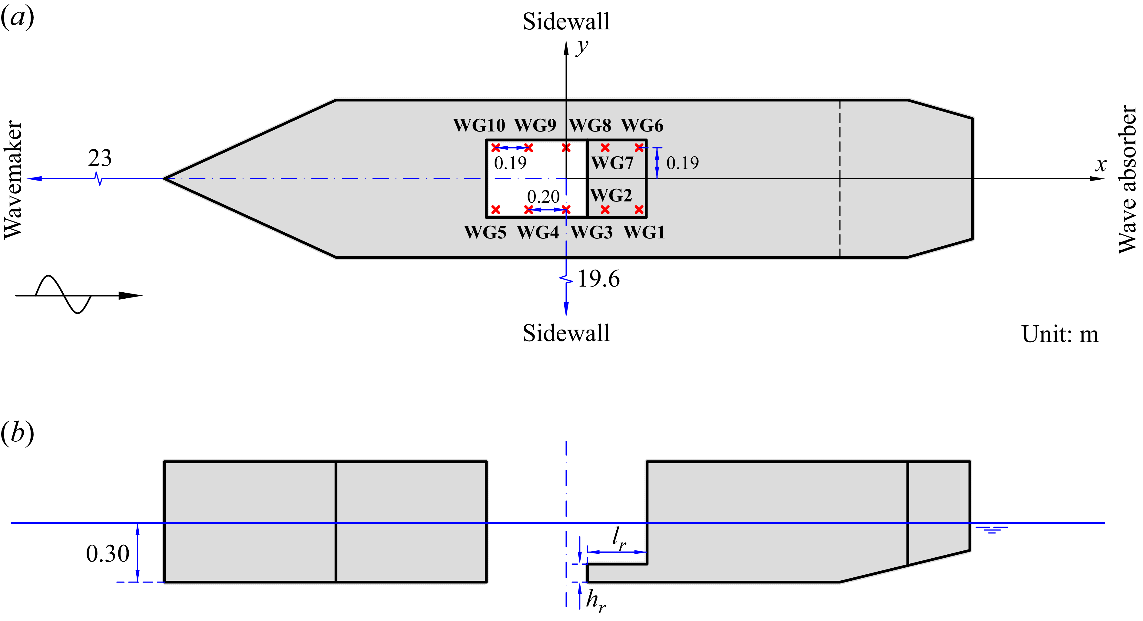


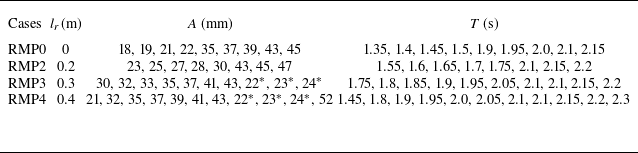


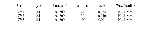


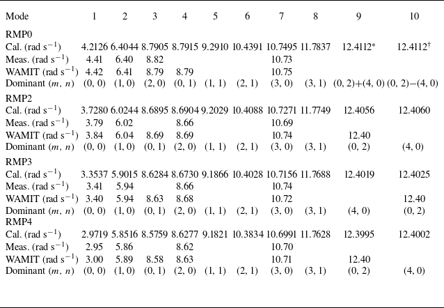


 Open access