





1. Introduction
In [Reference Okounkov15], Okounkov conjectured the log-concavity in large from statistical physics point of view, particularly, the structure constants for many interesting basis from representation theory. The recently developed Lorentzian polynomials [Reference Brändén and Huh1] help to solve many interesting cases (e.g., [Reference Huh, Matherne, Mészáros and St Dizier12]). We are interested in the log-concavity for the theta basis [Reference Gross, Hacking, Keel and Kontsevich10] of cluster algebras, which are not Lorentzian in general.
Cluster algebras are important commutative algebras with a distinguished set of generators. In [Reference Fomin and Zelevinsky5] and [Reference Fomin and Zelevinsky6], they were first introduced to investigate the total positivity of Lie groups and canonical bases of quantum groups. Nowadays, cluster algebras are closely related to different subjects in mathematics.
Later on, in [Reference Fock and Goncharov2] and [Reference Fock and Goncharov3], Fock and Goncharov generalized the cluster structure into the cluster ensemble structure for a pair of dual spaces $(\mathcal {X}^*, \mathcal {A})$
, and they conjectured that the tropical integer points of one space cluster modular group equivariantly parameterizes the canonical linear basis of the ring of regular functions on the dual space, and the highest term exponent of the regular function in cluster variables reflects the corresponding tropical point. Unfortunately, this conjecture is usually false due to the lack of global functions by [Reference Gross, Hacking and Keel9]. By the seminal work of Gross et al. [Reference Gross, Hacking, Keel and Kontsevich10], using scattering diagrams, broken lines, and theta functions, they proved the duality conjecture under certain conditions. By [Reference Mandel13], the theta functions are the atomic global Laurent polynomials of cluster variables.
$(\mathcal {X}^*, \mathcal {A})$
, and they conjectured that the tropical integer points of one space cluster modular group equivariantly parameterizes the canonical linear basis of the ring of regular functions on the dual space, and the highest term exponent of the regular function in cluster variables reflects the corresponding tropical point. Unfortunately, this conjecture is usually false due to the lack of global functions by [Reference Gross, Hacking and Keel9]. By the seminal work of Gross et al. [Reference Gross, Hacking, Keel and Kontsevich10], using scattering diagrams, broken lines, and theta functions, they proved the duality conjecture under certain conditions. By [Reference Mandel13], the theta functions are the atomic global Laurent polynomials of cluster variables.
When the cluster algebra is of finite type, the theta functions are exactly cluster monomials [Reference Gross, Hacking, Keel and Kontsevich10, Theorem 7.20]. Particularly for the cluster algebras of type $A_n$
, the theta basis is exactly the cluster monomial basis. Let us index the theta function
$A_n$
, the theta basis is exactly the cluster monomial basis. Let us index the theta function $\theta _i$
by the tropical point i. Then
$\theta _i$
by the tropical point i. Then
 $$ \begin{align}\theta_{i_1}\ldots \theta_{i_n}=\sum c_{i_1,\ldots,i_n}^j \theta_{j},\end{align} $$
where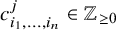 $c_{i_1,\ldots ,i_n}^j\in \mathbb {Z}_{\geq 0}$
. In [Reference Shen18], Shen proved that the support of the structure constants
$c_{i_1,\ldots ,i_n}^j\in \mathbb {Z}_{\geq 0}$
. In [Reference Shen18], Shen proved that the support of the structure constants $c_{i_1,\ldots ,i_n}^j$
is exactly a cluster convex hull of
$c_{i_1,\ldots ,i_n}^j$
is exactly a cluster convex hull of $i_1,\ldots ,i_n$
. Fix the cluster variables
$i_1,\ldots ,i_n$
. Fix the cluster variables $x_1,\ldots ,x_k$
of a seed. By Theorem 2.8, any theta function
$x_1,\ldots ,x_k$
of a seed. By Theorem 2.8, any theta function $\theta _c$
can be written as a polynomial
$\theta _c$
can be written as a polynomial $P_c$
of
$P_c$
of $x_1,\ldots ,x_k$
diving the theta function
$x_1,\ldots ,x_k$
diving the theta function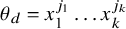 $\theta _d=x_1^{j_1}\ldots x_k^{j_k}$
, where
$\theta _d=x_1^{j_1}\ldots x_k^{j_k}$
, where $j_i\in \mathbb {Z}_{\geq 0}$
. Thus, the support of the coefficients of
$j_i\in \mathbb {Z}_{\geq 0}$
. Thus, the support of the coefficients of $\theta _c$
or
$\theta _c$
or $P_c$
is a cluster convex hull of
$P_c$
is a cluster convex hull of $c,d$
. We say that the structure constants
$c,d$
. We say that the structure constants $c_{i_1,\ldots ,i_n}^j$
are log-concave in j if for any cluster chart
$c_{i_1,\ldots ,i_n}^j$
are log-concave in j if for any cluster chart $\mathbb {R}^k$
of j, there is a log-concave function
$\mathbb {R}^k$
of j, there is a log-concave function $f(j)$
passing through all non-zero
$f(j)$
passing through all non-zero $c_{i_1,\ldots ,i_n}^j$
. To further understand these coefficients, we conjecture the following.
$c_{i_1,\ldots ,i_n}^j$
. To further understand these coefficients, we conjecture the following.
Conjecture 1.1. For certain cluster algebra including all the finite type cluster algebra, the structure constants $c_{i_1,\ldots ,i_n}^j$
of the theta basis are log-concave in j. Particularly, the coefficients of
$c_{i_1,\ldots ,i_n}^j$
of the theta basis are log-concave in j. Particularly, the coefficients of $\theta _c$
in the cluster variable of any given seed are log-concave.
$\theta _c$
in the cluster variable of any given seed are log-concave.
In this article, we focus on studying the cluster algebras of type $A_n$
. Recall that there is a geometric realization for them: triangulation. Afterward, Schiffler [Reference Schiffler16] provided an expansion formula of cluster variables by T-path (see Definition 3.2). Then, by use of the combinatorial and geometric information (intersection numbers) of T-path, we prove the main theorem as follows.
$A_n$
. Recall that there is a geometric realization for them: triangulation. Afterward, Schiffler [Reference Schiffler16] provided an expansion formula of cluster variables by T-path (see Definition 3.2). Then, by use of the combinatorial and geometric information (intersection numbers) of T-path, we prove the main theorem as follows.
Theorem 1.2 (Theorem 4.2).
All the cluster variables of cluster algebras of type $A_n$
are log-concave, that is, the coefficient-free cluster algebras of type
$A_n$
are log-concave, that is, the coefficient-free cluster algebras of type $A_n$
are log-concave.
$A_n$
are log-concave.
For the cluster algebras of type $A_2$
, we consider the corresponding cluster monomials. By use of binomial coefficients, we also prove the log-concavity of them as follows and give a conjecture for general cases (see Conjecture 5.5).
$A_2$
, we consider the corresponding cluster monomials. By use of binomial coefficients, we also prove the log-concavity of them as follows and give a conjecture for general cases (see Conjecture 5.5).
Theorem 1.3 (Theorem 5.3).
The cluster monomials of cluster algebras of type $A_2$
are log-concave.
$A_2$
are log-concave.
In the end, according to the geometric realization of d-vectors and the relations between d-vectors and f-vectors, we show the log-concavity of F-polynomials of type $A_n$
as follows.
$A_n$
as follows.
Theorem 1.4 (Theorem 6.8).
All the F-polynomials of cluster algebras of type $A_n$
are log-concave.
$A_n$
are log-concave.
It would also be very interesting to investigate Conjecture 1.1 for the general decorated surface cases.
The article is organized as follows: In Section 2, we recall the basic definitions of semifields, seeds, cluster algebras, and cluster monomials. Then, we introduce the definition of log-concavity of Laurent polynomials (Definition 2.17). In Section 3, we review the geometric realization of cluster algebras of type $A_n$
. In particular, by use of T-path, we prove Proposition 3.7. In Section 4, we prove the log-concavity of cluster variables of type
$A_n$
. In particular, by use of T-path, we prove Proposition 3.7. In Section 4, we prove the log-concavity of cluster variables of type $A_n$
based on the combinatorial and geometric information of T-path (see Theorem 4.2). In Section 5, by use of binomial coefficients, we prove that the cluster monomials of type
$A_n$
based on the combinatorial and geometric information of T-path (see Theorem 4.2). In Section 5, by use of binomial coefficients, we prove that the cluster monomials of type $A_2$
are log-concave (Theorem 5.3). In addition, we give a conjecture about type
$A_2$
are log-concave (Theorem 5.3). In addition, we give a conjecture about type $A_n(n\geq 3)$
(see Conjecture 5.5). Finally, in Section 6, we recall the definitions of F-polynomials and f-vectors. Then, by use of the relations between f-vectors and d-vectors, we prove the log-concavity of F-polynomials of type
$A_n(n\geq 3)$
(see Conjecture 5.5). Finally, in Section 6, we recall the definitions of F-polynomials and f-vectors. Then, by use of the relations between f-vectors and d-vectors, we prove the log-concavity of F-polynomials of type $A_n$
(Theorem 6.8).
$A_n$
(Theorem 6.8).
Conventions:
-
• In this article, the integer ring, the set of non-negative integers, the set of positive integers, and the rational number field are denoted by $\mathbb {Z}$
,
$\mathbb {N}$
,
$\mathbb {N}_{+}$
, and
$\mathbb {Q,}$
respectively.
$\mathbb {Z}$
,
$\mathbb {N}$
,
$\mathbb {N}_{+}$
, and
$\mathbb {Q,}$
respectively. -
• We denote by
$\text {Mat}_{n\times n}(\mathbb {Z})$
the set of all
$n\times n$
integer square matrices. An integer square matrix B is called skew-symmetrizable if there exists a positive integer diagonal matrix D such that
$DB$
is skew-symmetric and D is called the left skew-symmetrizer of B. -
• For any
$a\in \mathbb {Z}$
, we denote
$[a]_{+}=\max (a,0)$
. For any
$B=(b_{ij})_{n\times n}\in \text {Mat}_{n\times n}(\mathbb {Z})$
, we denote
$[B]_{+}=([b_{ij}]_{+})_{n\times n}$
. -
• Let
$B^{k\bullet }$
be the matrix obtained from B by replacing all entries outside of the kth row with zeros and
$B^{\bullet k}$
be the matrix obtained from B by replacing all entries outside of the kth column with zeros. We denote
$J_k$
the diagonal matrix obtained from the identity matrix by replacing the kth diagonal entry with
$-1$
.






2. Preliminaries
In this section, we recall some basic but important notions about cluster algebras as introduced by Fomin–Zelevinsky [Reference Fomin and Zelevinsky5–Reference Fomin and Zelevinsky7]. In addition, we introduce the definition of log-concavity of Laurent polynomials and their properties.
2.1. Semifields and cluster algebras
Firstly, in this section, we recall some definitions and properties of semifields and cluster algebras.
Definition 2.1 (Semifield).
A semifield is a multiplicative abelian group $(\mathbb {P},\cdot )$
which is equipped with an additive operation
$(\mathbb {P},\cdot )$
which is equipped with an additive operation $\oplus $
such that for any
$\oplus $
such that for any $a,b,c \in \mathbb {P}$
:
$a,b,c \in \mathbb {P}$
:
-
(1)
$a \oplus b=b \oplus a$
; -
(2)
$(a \oplus b)c = ac \oplus bc$
; -
(3)
$(a \oplus b) \oplus c = a \oplus (b \oplus c).$



Then, we denote it by $(\mathbb {P}, \cdot , \oplus )$
.
$(\mathbb {P}, \cdot , \oplus )$
.
Example 2.2. The following examples are two important semifields.
-
(1) Let
$\mathbb {P}_{\text {triv}}=\{1\}$
be a trivial multiplicative group equipped with addition
$\oplus $
such that
$1\oplus 1=1$
. Then,
$\mathbb {P}_{\text {triv}}$
becomes a semifield and it is called a trivial semifield. -
(2) Let
$\mathbb {P}_{\text {trop}}=\text {Trop}(u_1,\dots , u_n)$
be a multiplicative abelian group freely generated by formal variables
$u_1,\dots ,u_n$
with addition
$\oplus $
as follows: (2)
$$ \begin{align} \prod_{i=1}^n u_i^{a_i} \oplus \prod_{i=1}^{n} u_i^{b_i}=\prod_{i=1}^{n} u_j^{\min(a_i,b_i)}. \end{align} $$


Now, we fix $n\in \mathbb {N}_{+}$
. According to [Reference Fomin and Zelevinsky5], the group ring
$n\in \mathbb {N}_{+}$
. According to [Reference Fomin and Zelevinsky5], the group ring $\mathbb {Z}\mathbb {P}$
is a domain and we can construct its fractional field, which is denoted by
$\mathbb {Z}\mathbb {P}$
is a domain and we can construct its fractional field, which is denoted by $\mathbb {Q}\mathbb {P}$
. Let
$\mathbb {Q}\mathbb {P}$
. Let $\mathcal {F}$
be a rational function field with n indeterminates over
$\mathcal {F}$
be a rational function field with n indeterminates over $\mathbb {Q}\mathbb {P}$
and we call it the ambient field.
$\mathbb {Q}\mathbb {P}$
and we call it the ambient field.
Definition 2.3 (Seeds).
A labeled seed is a triple $(\mathbf {x},\mathbf {y},B)$
such that
$(\mathbf {x},\mathbf {y},B)$
such that $\mathbf {x}=(x_1,\dots ,x_n)$
is an n-tuple of algebraically independent generating elements of
$\mathbf {x}=(x_1,\dots ,x_n)$
is an n-tuple of algebraically independent generating elements of $\mathcal {F}$
,
$\mathcal {F}$
, $\mathbf {y}=(y_1,\dots ,y_{n})$
is an n-tuple of
$\mathbf {y}=(y_1,\dots ,y_{n})$
is an n-tuple of $\mathbb {P}$
and
$\mathbb {P}$
and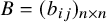 ${B=(b_{ij})_{n\times n}}$
is a skew-symmetrizable matrix. We call the n-tuple
${B=(b_{ij})_{n\times n}}$
is a skew-symmetrizable matrix. We call the n-tuple $\mathbf {x}$
cluster, the element
$\mathbf {x}$
cluster, the element $x_i$
cluster variable, the element
$x_i$
cluster variable, the element $y_i$
coefficient variable, and B the exchange matrix, respectively.
$y_i$
coefficient variable, and B the exchange matrix, respectively.
Furthermore, there is an important notion of the mutation of a seed.
Definition 2.4 (Seed mutations).
Let $(\mathbf {x},\mathbf {y},B)$
be a labeled seed and
$(\mathbf {x},\mathbf {y},B)$
be a labeled seed and $1\leq k\leq n$
, we define a new labeled seed
$1\leq k\leq n$
, we define a new labeled seed $\mu _k(\mathbf {x},\mathbf {y},B)=(\mathbf {x}^{\prime },\mathbf {y}^{\prime },B^{\prime })$
as follows:
$\mu _k(\mathbf {x},\mathbf {y},B)=(\mathbf {x}^{\prime },\mathbf {y}^{\prime },B^{\prime })$
as follows:
-
(1)
$\mathbf {x}^{\prime }=(x_{1}^{\prime },\dots ,x_{n}^{\prime })$
, where (3)
$$ \begin{align} x_{i}^{\prime}=\left\{ \begin{array}{ll} x_{k}^{-1}(\dfrac{y_{k}}{1 \oplus y_{k}}\prod\limits_{j=1}^{n}x_{j}^{[b_{jk}]_{+}}+\dfrac{1}{1 \oplus y_{k}}\prod\limits_{j=1}^{n}x_{j}^{[-b_{jk}]_{+}}), & i=k, \\ x_{i}, & i \neq k. \end{array} \right. \end{align} $$
-
(2)
$\mathbf {y}^{\prime }=(y_1^{\prime },\dots ,y_{n}^{\prime })$
, where (4)
$$ \begin{align} y_{i}^{\prime}=\left\{ \begin{array}{ll} y_{k}^{-1}, & i=k, \\ y_{i}y_{k}^{[b_{ki}]_{+}}(1\oplus y_{k})^{-b_{ki}}, & i \neq k. \end{array} \right. \end{align} $$
-
(3)
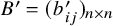
$B^{\prime }=(b_{ij}^{\prime })_{n\times n}$
is given by (5)
$$ \begin{align} b_{ij}^{\prime}=\left\{ \begin{array}{ll} -b_{ij}, & i=k \;\;\text{ or }\;\; j=k, \\ b_{ij}+[b_{ik}]_{+}b_{kj}+b_{ik}[-b_{kj}]_{+}, & i\neq k \;\; \text{ and }\; j\neq k. \end{array} \right. \end{align} $$





In fact, $(\mathbf {x}^{\prime },\mathbf {y}^{\prime },B^{\prime })$
is still a seed and
$(\mathbf {x}^{\prime },\mathbf {y}^{\prime },B^{\prime })$
is still a seed and $\mu _k$
is an involution, that is,
$\mu _k$
is an involution, that is, $\mu _k(\mathbf {x}^{\prime },\mathbf {y}^{\prime },B^{\prime })=(\mathbf {x},\mathbf {y},B)$
(see [Reference Nakanishi14]). Then,
$\mu _k(\mathbf {x}^{\prime },\mathbf {y}^{\prime },B^{\prime })=(\mathbf {x},\mathbf {y},B)$
(see [Reference Nakanishi14]). Then, $(\mathbf {x}^{\prime },\mathbf {y}^{\prime },B^{\prime })$
is called the k-direction mutation of
$(\mathbf {x}^{\prime },\mathbf {y}^{\prime },B^{\prime })$
is called the k-direction mutation of $(\mathbf {x},\mathbf {y},B)$
.
$(\mathbf {x},\mathbf {y},B)$
.
Remark 2.5. The coefficients were defined in [Reference Fomin and Zelevinsky5, Definition 5.3] and [Reference Fomin and Zelevinsky6, Section 1.2] as a $2n$
-tuple
$2n$
-tuple $\mathbf {p}=(p_1^{\pm 1},\dots ,p_n^{\pm 1})$
of
$\mathbf {p}=(p_1^{\pm 1},\dots ,p_n^{\pm 1})$
of $\mathbb {P}$
, such that
$\mathbb {P}$
, such that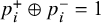 $p_i^{+}\oplus p_i^{-}=1$
for any
$p_i^{+}\oplus p_i^{-}=1$
for any $i\in \{1,\dots ,n\}$
. According to [Reference Fomin and Zelevinsky5, Formulas (5.2) and (5.3)], the two setups are equivalent by setting
$i\in \{1,\dots ,n\}$
. According to [Reference Fomin and Zelevinsky5, Formulas (5.2) and (5.3)], the two setups are equivalent by setting
 $$ \begin{align} y_i=\dfrac{p_i^{+}}{p_i^{-}}, \end{align} $$
and $p_i^{\pm 1}$
can be recovered by
$p_i^{\pm 1}$
can be recovered by
 $$ \begin{align} p_i^{+}=\dfrac{y_i}{y_i\oplus 1},\ p_i^{-}=\dfrac{1}{y_i\oplus 1}. \end{align} $$
Definition 2.6 (Cluster patterns).
A cluster pattern $\boldsymbol{\Sigma }=\{(\mathbf {x}_t,\mathbf {y}_t,B_t)|\ t\in \mathbb {T}_n\}$
is a collection of labeled seeds which are indexed by the vertices of n-regular tree
$\boldsymbol{\Sigma }=\{(\mathbf {x}_t,\mathbf {y}_t,B_t)|\ t\in \mathbb {T}_n\}$
is a collection of labeled seeds which are indexed by the vertices of n-regular tree $\mathbb {T}_{n}$
, such that
$\mathbb {T}_{n}$
, such that $(\mathbf {x}_{t^{\prime }},\mathbf {y}_{t^{\prime }},B_{t^{\prime }})=\mu _k(\mathbf {x}_t,\mathbf {y}_t,B_t)$
for any
$(\mathbf {x}_{t^{\prime }},\mathbf {y}_{t^{\prime }},B_{t^{\prime }})=\mu _k(\mathbf {x}_t,\mathbf {y}_t,B_t)$
for any $t \stackrel {k}{\longleftrightarrow } t^{\prime }$
in
$t \stackrel {k}{\longleftrightarrow } t^{\prime }$
in $\mathbb {T}_n$
. In the following, we use the notations that
$\mathbb {T}_n$
. In the following, we use the notations that
 $$ \begin{align*}\mathbf{x}_{t}=(x_{1;t},\dots,x_{n;t}),\ \mathbf{y}_{t}=(y_{1;t},\dots,y_{n;t}),\ B_{t}=(b_{ij;t})_{n\times n}.\end{align*} $$
For an arbitrary fixed vertex $t_0\in \mathbb {T}_n$
, we call the seed
$t_0\in \mathbb {T}_n$
, we call the seed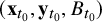 $(\mathbf {x}_{t_0},\mathbf {y}_{t_0},B_{t_0})$
initial seed and denote the initial cluster by
$(\mathbf {x}_{t_0},\mathbf {y}_{t_0},B_{t_0})$
initial seed and denote the initial cluster by $\mathbf {x}_{t_0}=\mathbf {x}=(x_{1},\dots ,x_{n})$
, the initial coefficients by
$\mathbf {x}_{t_0}=\mathbf {x}=(x_{1},\dots ,x_{n})$
, the initial coefficients by $\mathbf {y}_{t_0}=\mathbf {y}=(y_{1},\dots ,y_{n}),$
and the initial exchange matrix by
$\mathbf {y}_{t_0}=\mathbf {y}=(y_{1},\dots ,y_{n}),$
and the initial exchange matrix by $B_{t_0}=B=(b_{ij})_{n\times n}$
.
$B_{t_0}=B=(b_{ij})_{n\times n}$
.
Now, we are ready to define the crucial notions of cluster algebras.
Definition 2.7 (Cluster algebras).
For a cluster pattern $\boldsymbol{\Sigma }$
, the cluster algebra
$\boldsymbol{\Sigma }$
, the cluster algebra $\mathcal {A}=\mathcal {A}(\boldsymbol{\Sigma })$
is the
$\mathcal {A}=\mathcal {A}(\boldsymbol{\Sigma })$
is the $\mathbb {Z}\mathbb {P}$
-subalgebra of
$\mathbb {Z}\mathbb {P}$
-subalgebra of $\mathcal {F}$
generated by all the cluster variables
$\mathcal {F}$
generated by all the cluster variables $\{x_{i;t}\mid i=1,\dots ,n;t\in \mathbb {T}_{n}\}$
. Here, n is called the rank of
$\{x_{i;t}\mid i=1,\dots ,n;t\in \mathbb {T}_{n}\}$
. Here, n is called the rank of $\mathcal {A}$
or
$\mathcal {A}$
or $\boldsymbol{\Sigma }$
.
$\boldsymbol{\Sigma }$
.
Furthermore, if $\mathbb {P}=\mathbb {P}_{\text {trop}}=\text {Trop}(x_{n+1},\dots , x_m)$
, then
$\mathbb {P}=\mathbb {P}_{\text {trop}}=\text {Trop}(x_{n+1},\dots , x_m)$
, then $\mathcal {A}$
is called of geometric type. If
$\mathcal {A}$
is called of geometric type. If $\mathbb {P}=\mathbb {P}_{\text {triv}}$
, then
$\mathbb {P}=\mathbb {P}_{\text {triv}}$
, then $\mathcal {A}$
is said to be coefficient-free or with trivial coefficients. In this case, the seed
$\mathcal {A}$
is said to be coefficient-free or with trivial coefficients. In this case, the seed $(\mathbf {x},\mathbf {y},B)$
can be reduced to
$(\mathbf {x},\mathbf {y},B)$
can be reduced to $(\mathbf {x},B)$
. Furthermore,
$(\mathbf {x},B)$
. Furthermore, $\mathbb {Z}\mathbb {P}$
and
$\mathbb {Z}\mathbb {P}$
and $\mathbb {Q}\mathbb {P}$
can be reduced to
$\mathbb {Q}\mathbb {P}$
can be reduced to $\mathbb {Z}$
and
$\mathbb {Z}$
and $\mathbb {Q}$
, respectively, that is, the cluster algebra
$\mathbb {Q}$
, respectively, that is, the cluster algebra $\mathcal {A}$
is a
$\mathcal {A}$
is a $\mathbb {Z}$
-subalgebra of
$\mathbb {Z}$
-subalgebra of $\mathcal {F}$
generated by all the cluster variables.
$\mathcal {F}$
generated by all the cluster variables.
Theorem 2.8 ([Reference Fomin and Zelevinsky5, Theorem 3.1], [Reference Gross, Hacking, Keel and Kontsevich10, Theorem 4.10]).
In a cluster algebra $\mathcal {A}$
, any cluster variable is a Laurent polynomial in terms of the initial cluster with coefficients in
$\mathcal {A}$
, any cluster variable is a Laurent polynomial in terms of the initial cluster with coefficients in $\mathbb {N}\mathbb {P}$
.
$\mathbb {N}\mathbb {P}$
.
More precisely, we have the Laurent expression of $x_{i;t}$
in terms of the initial cluster
$x_{i;t}$
in terms of the initial cluster $\mathbf {x}=(x_1,\dots ,x_n)$
as follows:
$\mathbf {x}=(x_1,\dots ,x_n)$
as follows:
 $$ \begin{align} x_{i;t}=\dfrac{N_{i;t}(x_1,\dots, x_n)}{x_1^{d_{1i;t}}\dots x_n^{d_{ni;t}}},\ d_{ji;t}\in \mathbb{Z}, \end{align} $$
where $N_{i;t}(x_1,\dots , x_n)$
is a polynomial with coefficients in
$N_{i;t}(x_1,\dots , x_n)$
is a polynomial with coefficients in $\mathbb {N}\mathbb {P}$
which is not divisible by any
$\mathbb {N}\mathbb {P}$
which is not divisible by any $x_j$
. The integer vector
$x_j$
. The integer vector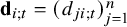 $\mathbf {d}_{i;t}=(d_{ji;t})_{j=1}^n$
is called the denominator vector (d-vector) of
$\mathbf {d}_{i;t}=(d_{ji;t})_{j=1}^n$
is called the denominator vector (d-vector) of $x_{i;t}$
. In fact, the recurrence relations for
$x_{i;t}$
. In fact, the recurrence relations for $\mathbf {d}$
-vectors are given as follows (cf. [Reference Fomin and Zelevinsky7, Section 4.3]). The initial conditions are
$\mathbf {d}$
-vectors are given as follows (cf. [Reference Fomin and Zelevinsky7, Section 4.3]). The initial conditions are $\mathbf {d}_{l;t_0}=-\mathbf {e}_{l}$
and the recursion formula is
$\mathbf {d}_{l;t_0}=-\mathbf {e}_{l}$
and the recursion formula is
 $$ \begin{align} \mathbf{d}_{l;t^{\prime}}=\left\{ \begin{array}{ll} \mathbf{d}_{l;t}, & l\neq k, \\ -\mathbf{d}_{k;t}+\text{max}\ (\sum\limits_{i=1}^n[b_{ik;t}]_{+}\mathbf{d}_{i;t},\sum\limits_{i=1}^n[-b_{ik;t}]_{+}\mathbf{d}_{i;t}), & l=k, \end{array} \right. \end{align} $$
for $t \stackrel {k}{\longleftrightarrow } t^{\prime }$
in
$t \stackrel {k}{\longleftrightarrow } t^{\prime }$
in $\mathbb {T}_n$
.
$\mathbb {T}_n$
.
Definition 2.9 (Finite type).
A cluster algebra $\mathcal {A}$
is called of finite type if it contains finitely many distinct seeds. Otherwise, it is called of infinite type.
$\mathcal {A}$
is called of finite type if it contains finitely many distinct seeds. Otherwise, it is called of infinite type.
Let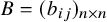 $B=(b_{ij})_{n\times n}$
be a skew-symmetrizable integer matrix whose Cartan counterpart is a symmetrizable generalized Cartan matrix
$B=(b_{ij})_{n\times n}$
be a skew-symmetrizable integer matrix whose Cartan counterpart is a symmetrizable generalized Cartan matrix $A=A(B)=(a_{ij})_{n\times n}$
, where
$A=A(B)=(a_{ij})_{n\times n}$
, where
 $$ \begin{align} a_{ij}=\left\{ \begin{array}{ll} 2, & i=j, \\ -|b_{ij}|, & i \neq j. \end{array} \right. \end{align} $$
Theorem 2.10 [Reference Fomin and Zelevinsky6, Theorem 1.8].
A cluster algebra is of finite type if and only if it contains an exchange matrix B whose Cartan counterpart $A(B)$
is a Cartan matrix of finite type.
$A(B)$
is a Cartan matrix of finite type.
In particular, when the cluster algebra $\mathcal {A}$
is of rank
$\mathcal {A}$
is of rank $2$
, whose initial exchange matrix is given by
$2$
, whose initial exchange matrix is given by
 $$ \begin{align} \begin{pmatrix} 0 & b \\ -c & 0 \end{pmatrix}, \end{align} $$
where $b,c \in \mathbb {N}$
. Then, it is of finite type if and only if
$b,c \in \mathbb {N}$
. Then, it is of finite type if and only if $0\leq bc\leq 3$
. If
$0\leq bc\leq 3$
. If $bc=4$
, the cluster algebra
$bc=4$
, the cluster algebra $\mathcal {A}$
is called of affine type. If
$\mathcal {A}$
is called of affine type. If $bc\geq 5$
, it is called of non-affine type.
$bc\geq 5$
, it is called of non-affine type.
Definition 2.11 (Dynkin type).
Let $X_n\ (\text {e.g.,}\,A_n, B_n, \dots )$
be a Dynkin diagram with n vertices. A cluster algebra
$X_n\ (\text {e.g.,}\,A_n, B_n, \dots )$
be a Dynkin diagram with n vertices. A cluster algebra $\mathcal {A}$
is called of type
$\mathcal {A}$
is called of type $X_n$
if one of its exchange matrices B has Cartan counterpart of type
$X_n$
if one of its exchange matrices B has Cartan counterpart of type $X_n$
.
$X_n$
.
Remark 2.12. The cluster algebra $\mathcal {A}$
is of type
$\mathcal {A}$
is of type $A_n, D_n, E_6, E_7$
, or
$A_n, D_n, E_6, E_7$
, or $E_8$
if and only if one of its exchange matrices B corresponds to a quiver which is an orientation of a Dynkin diagram of the type above.
$E_8$
if and only if one of its exchange matrices B corresponds to a quiver which is an orientation of a Dynkin diagram of the type above.
There is another crucial notion of cluster monomials.
Definition 2.13 (Cluster monomials).
A cluster monomial is a product of non-negative powers of cluster variables which all belong to a same cluster. More precisely, for any $t\in \mathbb {T}_n$
, the set of cluster monomials is
$t\in \mathbb {T}_n$
, the set of cluster monomials is $\{x_{1;t}^{m_1}\dots x_{n;t}^{m_n}\mid m_1,\dots ,m_n\in \mathbb {Z}_{\geq 0}\}$
.
$\{x_{1;t}^{m_1}\dots x_{n;t}^{m_n}\mid m_1,\dots ,m_n\in \mathbb {Z}_{\geq 0}\}$
.
The notion of cluster monomials plays an important role in cluster theory. In [Reference Gross, Hacking, Keel and Kontsevich10, Theorem 7.20], it was proved that for a cluster algebra, all distinct cluster monomials are linearly independent over $\mathbb {Z}$
. In addition, the cluster monomials are contained in the theta functions. When the cluster algebra is of finite type, theta functions are strictly cluster monomials. Here, for brevity, we do not recall the definition of theta functions.
$\mathbb {Z}$
. In addition, the cluster monomials are contained in the theta functions. When the cluster algebra is of finite type, theta functions are strictly cluster monomials. Here, for brevity, we do not recall the definition of theta functions.
Example 2.14 (Coefficient-free
$A_2$
type.)

Let $(\mathbf {x},B)$
be the initial seed, where
$(\mathbf {x},B)$
be the initial seed, where
 $$ \begin{align} \mathbf{x}=(x_1,x_2),\ B=\begin{pmatrix}0 & 1\\ -1 & 0\end{pmatrix}. \end{align} $$
Note that the (labeled) clusters are 10-periodic and they are as follows:
 $$ \begin{align*}\begin{array}{c} \left(x_1,x_2\right),\ \left(\dfrac{x_2+1}{x_1},x_2\right),\ \left(\dfrac{x_2+1}{x_1},\dfrac{x_1+x_2+1}{x_1x_2}\right),\ \left(\dfrac{x_1+1}{x_2},\dfrac{x_1+x_2+1}{x_1x_2}\right),\ \left(\dfrac{x_1+1}{x_2},x_1\right),\\\\[-6pt] \left(x_2,x_1\right),\ \left(x_2,\dfrac{x_2+1}{x_1}\right),\ \left(\dfrac{x_1+x_2+1}{x_1x_2},\dfrac{x_2+1}{x_1}\right),\ \left(\dfrac{x_1+x_2+1}{x_1x_2},\dfrac{x_1+1}{x_2}\right),\ \left(x_1,\dfrac{x_1+1}{x_2}\right). \end{array}\end{align*} $$
Hence, there are five classes of cluster monomials:
 $$ \begin{align*}\begin{array}{l} x_1^{m_1}x_2^{m_2}, \left(\dfrac{x_2+1}{x_1}\right)^{m_1}x_2^{m_2}, \left(\dfrac{x_2+1}{x_1}\right)^{m_1}\left(\dfrac{x_1+x_2+1}{x_1x_2}\right)^{m_2}, \left(\dfrac{x_1+1}{x_2}\right)^{m_1}\left(\dfrac{x_1+x_2+1}{x_1x_2}\right)^{m_2}, \left(\dfrac{x_1+1}{x_2}\right)^{m_1}\left(x_1\right)^{m_2}, \end{array}\end{align*} $$
where $m_1,m_2 \in \mathbb {Z}_{\geq 0}$
.
$m_1,m_2 \in \mathbb {Z}_{\geq 0}$
.
Remark 2.15. Note that the cluster monomials of type $A_2$
are independent of the choices of the initial exchange matrix. That is, if the initial exchange matrix is
$A_2$
are independent of the choices of the initial exchange matrix. That is, if the initial exchange matrix is $-B$
, then the cluster monomials are the same as above. However, the cases of type
$-B$
, then the cluster monomials are the same as above. However, the cases of type $A_n\ (n\geq 3)$
are quite different.
$A_n\ (n\geq 3)$
are quite different.
2.2. Log-concavity of Laurent polynomials
In this section, we introduce the notion of Laurent polynomials and its relation with concave functions.
Definition 2.16 (Concave functions).
Let $\Omega \subseteq \mathbb {R}^{m}$
be a convex set. A function
$\Omega \subseteq \mathbb {R}^{m}$
be a convex set. A function $f(x_1,\dots ,x_m): \Omega \rightarrow \mathbb {R}$
is said to be concave if for any
$f(x_1,\dots ,x_m): \Omega \rightarrow \mathbb {R}$
is said to be concave if for any $\mathbf {x}, \mathbf {y} \in \Omega $
and
$\mathbf {x}, \mathbf {y} \in \Omega $
and $\lambda \in [0,1]$
, then
$\lambda \in [0,1]$
, then
 $$ \begin{align}f((1-\lambda)\mathbf{x}+\lambda\mathbf{y})\geq (1-\lambda)f(\mathbf{x})+\lambda f(\mathbf{y}).\end{align} $$
Definition 2.17 (Log-concavity of Laurent polynomials).
A nonzero Laurent polynomial with non-negative real coefficients and m variables
 $$ \begin{align}f(x_1,\dots,x_m)=\sum\limits_{i_1=l_1}^{n_1}\dots\sum\limits_{i_m=l_m}^{n_m}a_{i_1,\dots,i_m}x_1^{i_1}\dots x_m^{i_m} \end{align} $$
is called log-concave if for any $1\leq j\leq m$
and
$1\leq j\leq m$
and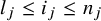 $l_j\leq i_j\leq n_j$
,
$l_j\leq i_j\leq n_j$
,
 $$ \begin{align}a^2_{i_1,\dots,i_j,\dots,i_m}\geq a_{i_1,\dots,i_{j}-1,\dots,i_m}a_{i_1,\dots,i_{j}+1,\dots,i_m},\end{align} $$
where setting $a_{i_1,\dots ,l_j-1,\dots ,i_m}=a_{i_1,\dots ,n_{j}+1,\dots ,i_m}=0$
.
$a_{i_1,\dots ,l_j-1,\dots ,i_m}=a_{i_1,\dots ,n_{j}+1,\dots ,i_m}=0$
.
Example 2.18. There are several examples and counter-examples as follows:
-
(1) The polynomial with one variable
$f(x)=(x+1)^n$
is log-concave since the binomial coefficients
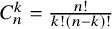
$C_n^k=\frac {n!}{k!(n-k)!}$
satisfy that (16)
$$ \begin{align} \frac{(C_n^k)^2}{C_n^{k-1}C_n^{k+1}}=\frac{(n-k+1)(k+1)}{(n-k)k}> 1. \end{align} $$
Note that
$x+1$
is log-concave, but
$x^2+1$
is not log-concave. -
(2) The Laurent polynomial with three variables
(17)is log-concave by direct calculation. In fact, it is a cluster variable of type
$$ \begin{align}f(x_1,x_2,x_3)=\dfrac{1+2x_2+x_2^2+x_1x_3}{x_1x_2x_3}\end{align} $$
$A_3$
(see Example 3.5).



Remark 2.19. Note that any two Laurent polynomials which are the same up to a Laurent monomial factor keep the same property of log-concavity. In particular, when the cluster algebra is coefficient-free, by formula (8), $x_{i;t}$
is log-concave if and only if
$x_{i;t}$
is log-concave if and only if $N_{i;t}(x_1,\dots ,x_n)$
is log-concave.
$N_{i;t}(x_1,\dots ,x_n)$
is log-concave.
For the nonzero Laurent polynomial (14), let $I=\{(i_1,\dots ,i_m)\in \mathbb {Z}^m|\ a_{i_1,\dots ,i_m}>0 \}$
and then it is a non-empty set. If the three consecutive terms with respect to (15) all belong to I, we take the logarithm and have
$I=\{(i_1,\dots ,i_m)\in \mathbb {Z}^m|\ a_{i_1,\dots ,i_m}>0 \}$
and then it is a non-empty set. If the three consecutive terms with respect to (15) all belong to I, we take the logarithm and have
 $$ \begin{align} \ln(a_{i_1,\dots,i_j,\dots,i_m})\geq \dfrac{1}{2}\ln(a_{i_1,\dots,i_{j}-1,\dots,i_m})+\dfrac{1}{2}\ln(a_{i_1,\dots,i_{j}+1,\dots,i_m}).\end{align} $$
Hence, it is direct that Definition 2.17 can be defined equivalently by a concave function passing through some integer points as follows.
Lemma 2.20. The nonzero Laurent polynomial with non-negative real coefficients (14) is log-concave if and only if there exists a function $g(x_1,\dots ,x_n):\Omega \rightarrow \mathbb {R}_{> 0}$
, where
$g(x_1,\dots ,x_n):\Omega \rightarrow \mathbb {R}_{> 0}$
, where $\Omega $
is a convex set containing I such that:
$\Omega $
is a convex set containing I such that:
-
(1) If
$a_{i_1,\dots ,i_j-1,\dots ,i_m}a_{i_1,\dots ,i_j+1,\dots ,i_m}>0$
, then
$a_{i_1,\dots ,i_j,\dots ,i_m}>0$
. -
(2)
$g(i_1,\dots ,i_m)=a_{i_1,\dots ,i_m}$
, where
$(i_1,\dots ,i_m)\in I$
. -
(3)
$G(\mathbf {x})=\ln (g(x_1,\dots ,x_m))$
is concave over
$\Omega $
.






3. Geometric realization of cluster algebras of type
$A_n$

In this section, we recall some basic notions of geometric realization of cluster algebras of type $A_n$
based on [Reference Fomin and Zelevinsky6]. We also recall a crucial expansion formula of cluster variables of type
$A_n$
based on [Reference Fomin and Zelevinsky6]. We also recall a crucial expansion formula of cluster variables of type $A_n$
by use of T-path, which is given by Schiffler [Reference Schiffler16] and Schiffler and Thomas [Reference Schiffler and Thomas17].
$A_n$
by use of T-path, which is given by Schiffler [Reference Schiffler16] and Schiffler and Thomas [Reference Schiffler and Thomas17].
3.1. Triangulation of
$(n+3)$
-gons

In the following, let $\mathcal {P}_{n+3}$
be a convex polygon with
$\mathcal {P}_{n+3}$
be a convex polygon with $n+3$
vertices. A boundary is a line segment connecting two adjacent vertices of
$n+3$
vertices. A boundary is a line segment connecting two adjacent vertices of $\mathcal {P}_{n+3}$
. A diagonal is a line segment connecting two non-adjacent vertices of
$\mathcal {P}_{n+3}$
. A diagonal is a line segment connecting two non-adjacent vertices of $\mathcal {P}_{n+3}$
. Two diagonals are called crossing if they intersect in the interior of
$\mathcal {P}_{n+3}$
. Two diagonals are called crossing if they intersect in the interior of $\mathcal {P}_{n+3}$
. A triangulation T of
$\mathcal {P}_{n+3}$
. A triangulation T of $\mathcal {P}_{n+3}$
is a maximal set of non-crossing diagonals together with all the boundary edges. Hence, there are n diagonals and
$\mathcal {P}_{n+3}$
is a maximal set of non-crossing diagonals together with all the boundary edges. Hence, there are n diagonals and $n+3$
boundary edges in a triangulation T. The boundary edges of
$n+3$
boundary edges in a triangulation T. The boundary edges of $\mathcal {P}_{n+3}$
are denoted by
$\mathcal {P}_{n+3}$
are denoted by $T_{n+1},\ldots ,T_{2n+3}$
.
$T_{n+1},\ldots ,T_{2n+3}$
.
According to [Reference Fomin and Zelevinsky6], in a cluster algebra of type $A_n$
, the clusters are in bijection with triangulations of
$A_n$
, the clusters are in bijection with triangulations of $\mathcal {P}_{n+3}$
. For a triangulation
$\mathcal {P}_{n+3}$
. For a triangulation $T=\{T_1,\ldots ,T_n,T_{n+1},\ldots ,T_{2n+3}\}$
, let
$T=\{T_1,\ldots ,T_n,T_{n+1},\ldots ,T_{2n+3}\}$
, let $\mathbf {x}=\mathbf {x}_{T}=\{x_1,\ldots ,x_n\}$
be the corresponding initial cluster, where we denote
$\mathbf {x}=\mathbf {x}_{T}=\{x_1,\ldots ,x_n\}$
be the corresponding initial cluster, where we denote $x_i=x_{T_i} $
. Moreover, take the semifield
$x_i=x_{T_i} $
. Moreover, take the semifield ${\mathbb {P}=\text {Trop}(x_{n+1},\dots ,x_{2n+3})}$
. Then, for any
${\mathbb {P}=\text {Trop}(x_{n+1},\dots ,x_{2n+3})}$
. Then, for any $1\leq k\leq n$
, the k-direction mutation exchange relation is given by
$1\leq k\leq n$
, the k-direction mutation exchange relation is given by
 $$ \begin{align} x_kx_{k^{\prime}}=x_ax_c+x_bx_d, \end{align} $$
where $T_a,T_c$
are two opposite edges of the quadrilateral and
$T_a,T_c$
are two opposite edges of the quadrilateral and $T_b,T_d$
are the other two opposite edges. The mutation can also be described as a flip of diagonals in the quadrilateral and the relation is usually called ptolemy relation (see Figure 1). We also associate an
$T_b,T_d$
are the other two opposite edges. The mutation can also be described as a flip of diagonals in the quadrilateral and the relation is usually called ptolemy relation (see Figure 1). We also associate an $n\times n$
matrix
$n\times n$
matrix $B=B(T)=(b_{ij}(T))_{n\times n}$
with the triangulation T as follows:
$B=B(T)=(b_{ij}(T))_{n\times n}$
with the triangulation T as follows:
 $$ \begin{align} b_{ij}(T)=\left\{ \begin{array}{ll} 1, & \text{If } T_i \text{and } T_j \text{ belong to a same triangle,}\\ &\text{and the rotation from } T_i \text{ to } T_j \text{ is counter-clockwise}; \\ -1, & \text{If } T_i \text{ and } T_j \text{ belong to a same triangle,}\\ &\text{and the rotation from } T_i \text{ to } T_j \text{ is clockwise};\\ 0, & \text{If } T_i \text{ and } T_j \text{ do not belong to a same triangle.} \end{array} \right. \end{align} $$
A flip in a quadrilateral.

We can also define the element $b_{ij}$
for
$b_{ij}$
for $n+1\leq i\leq 2n+3$
and
$n+1\leq i\leq 2n+3$
and $1\leq j\leq n$
as above. Then, the corresponding coefficient
$1\leq j\leq n$
as above. Then, the corresponding coefficient $2n$
-tuple
$2n$
-tuple $\mathbf {p}=(p_1^+,p_1^-,\dots ,p_n^+,p_n^-)$
is given by
$\mathbf {p}=(p_1^+,p_1^-,\dots ,p_n^+,p_n^-)$
is given by
 $$ \begin{align}p_i^+=\prod_{j\,\geq\, n+1 \,: \, b_{ji}=1 } x_j \qquad \text{and} \qquad p_i^-=\prod_{j\,\geq\, n+1 \,: \, b_{ji}=-1} x_j.\end{align} $$
Example 3.1. The zigzag triangulation of $6$
-gon in Figure 2 corresponds to the initial seed
$6$
-gon in Figure 2 corresponds to the initial seed $(\mathbf {x},\mathbf {p},B)$
of type
$(\mathbf {x},\mathbf {p},B)$
of type $A_3$
, where
$A_3$
, where
 $$ \begin{align} \mathbf{x}=(x_1,x_2,x_3),\ B=\begin{pmatrix}0 & -1 & 0 \\ 1 & 0 & 1 \\ 0 & -1 & 0\end{pmatrix}, \end{align} $$
and $\mathbf {p}=(p_1^+,p_1^-,p_2^+,p_2^-,p_3^+,p_3^-)$
is as follows:
$\mathbf {p}=(p_1^+,p_1^-,p_2^+,p_2^-,p_3^+,p_3^-)$
is as follows:
 $$ \begin{align} (p_1^+,p_1^-)=(x_4,x_5x_9),\ (p_2^+,p_2^-)=(x_6x_9,1),\ (p_3^+,p_3^-)=(x_7,x_6x_8). \end{align} $$
Note that $p_i^+ \oplus p_i^-=1$
for any
$p_i^+ \oplus p_i^-=1$
for any $i\in \{1,2,3\}$
. Then by Remark 2.5, the initial coefficient variables are
$i\in \{1,2,3\}$
. Then by Remark 2.5, the initial coefficient variables are
 $$ \begin{align}\mathbf{y}=(y_1,y_2,y_3)=(x_4x_5^{-1}x_9^{-1},x_6x_9,x_7x_6^{-1}x_8^{-1}).\end{align} $$
A triangulation of $6$
-gon (type
$6$
-gon (type $A_3$
).
$A_3$
).

3.2. T-paths
Let $T=\{T_1,\ldots ,T_n,T_{n+1},\ldots ,T_{2n+3}\}$
be an arbitrary triangulation of the convex
$T=\{T_1,\ldots ,T_n,T_{n+1},\ldots ,T_{2n+3}\}$
be an arbitrary triangulation of the convex $(n+3)$
-polygon
$(n+3)$
-polygon $\mathcal {P}_{n+3}$
, where
$\mathcal {P}_{n+3}$
, where $T_1,\ldots ,T_n$
are diagonals and
$T_1,\ldots ,T_n$
are diagonals and $T_{n+1},\ldots ,T_{2n+3}$
are boundaries. Let a and b be two non-adjacent vertices on the boundary and
$T_{n+1},\ldots ,T_{2n+3}$
are boundaries. Let a and b be two non-adjacent vertices on the boundary and $X_{a,b}$
be the diagonal between them.
$X_{a,b}$
be the diagonal between them.
Definition 3.2 (T-paths).
A T-path $\mathcal {P}$
from a to b is a sequence
$\mathcal {P}$
from a to b is a sequence
 $$\begin{align*}\mathcal{P} = (v_0,v_1,\ldots,v_{\ell(\mathcal{P})}\mid i_1,i_2,\ldots,i_{\ell(\mathcal{P})})\end{align*}$$
such that:
-
(T1)
$a=v_0,v_1,\dots ,v_{\ell (\mathcal {P})}=b$
are vertices of
$\mathcal {P}$
. -
(T2)
$T_{i_k}$
connects the vertices
$v_{{k-1}}$
and
$v_{k}$
for each
$k=1,2,\dots ,\ell (\mathcal {P})$
, where
$T_{i_k}\in T$
. -
(T3) If
$j\ne k$
, then
$i_j\ne i_k$
. -
(T4)
$\ell (\mathcal {P})$
is odd. -
(T5) If k is even, then
$T_{i_{k}}$
crosses
$X_{a,b}$
. -
(T6) If
$j<k$
and both
$T_{i_j}$
and
$T_{i_{k}}$
cross
$X_{a,b}$
then the crossing point of
$T_{i_j}$
and
$X_{a,b}$
is closer to the vertex
$ a $
than the crossing point of
$T_{i_{k}}$
and
$X_{a,b}$
.Figure 3Two possible cases of two symmetric T-paths.





Let $\mathcal {P}_T(a,b)$
be the set of all T-paths from a to b. In the following, in any T-path
$\mathcal {P}_T(a,b)$
be the set of all T-paths from a to b. In the following, in any T-path $\mathcal {P}$
from a to b, we classify the edges
$\mathcal {P}$
from a to b, we classify the edges $T_{i_k}$
as follows:
$T_{i_k}$
as follows:
-
• o: The diagonals which are passed through at odd steps.
-
• e: The diagonals which are passed through at even steps.
-
•
$\widetilde {o}$
: The boundaries which are passed through at odd steps.

For example, we can see these notations in Figure 3. For any T-path $\mathcal {P}$
from a to b, we associate a Laurent monomial
$\mathcal {P}$
from a to b, we associate a Laurent monomial $x(\mathcal {P})$
in the cluster algebra
$x(\mathcal {P})$
in the cluster algebra $\mathcal {A}$
of type
$\mathcal {A}$
of type $A_n$
as follows:
$A_n$
as follows:
 $$ \begin{align} x(\mathcal{P})= {\prod_{k \text{ odd }} x_{i_{k}}} \ {\prod_{k \text{ even }}x_{i_{k}}^{-1}}. \end{align} $$
Moreover, each cluster variable can be expressed by the sum of all such Laurent monomials $x(\mathcal {P})$
.
$x(\mathcal {P})$
.
Theorem 3.3 [Reference Schiffler16, Theorem 1.2].
Let a and b be two non-adjacent vertices of $\mathcal {P}_{n+3}$
,
$\mathcal {P}_{n+3}$
, $X_{a,b}$
be the diagonal between them, and
$X_{a,b}$
be the diagonal between them, and $x_{a,b}$
be the corresponding cluster variable. Then
$x_{a,b}$
be the corresponding cluster variable. Then
 $$ \begin{align} x_{a,b}=\sum_{\mathcal{P}\in\mathcal{P}_T(a,b)} x(\mathcal{P}). \end{align} $$
Remark 3.4. Formula (26) also holds for the coefficient-free cluster algebras of type $A_n$
when setting
$A_n$
when setting $x_i=1$
, where
$x_i=1$
, where $i=n+1, \dots ,2n+3$
.
$i=n+1, \dots ,2n+3$
.
Example 3.5. All the T-paths from a to b in Figure 2 are as follows (see Table 1). Hence, the coefficient-free cluster variable corresponding to the diagonal $ab$
in a cluster algebra of type
$ab$
in a cluster algebra of type $A_3$
is
$A_3$
is
 $$ \begin{align} x_{a,b}=\dfrac{x_2^2+2x_2+1+x_1x_3}{x_1x_2x_3}. \end{align} $$
It is clear that $x_{a,b}$
is log-concave with respect to each
$x_{a,b}$
is log-concave with respect to each $x_i$
.
$x_i$
.
T-paths from a to b in a cluster algebra of type $A_3$
$A_3$

Lemma 3.6 [Reference Schiffler16, Corollary 1.7].
Let $\mathcal {A}$
be a cluster algebra of type
$\mathcal {A}$
be a cluster algebra of type $A_n$
with coefficients
$A_n$
with coefficients ${\mathbb {P}=\text {Trop}(x_{n+1},\dots ,x_{2n+3})}$
and
${\mathbb {P}=\text {Trop}(x_{n+1},\dots ,x_{2n+3})}$
and $\mathbf {x}=\{x_1,\ldots ,x_n\}$
be the initial cluster. Let
$\mathbf {x}=\{x_1,\ldots ,x_n\}$
be the initial cluster. Let
 $$ \begin{align}x_{i;t}=\dfrac{N_{i;t}(x_1,\dots, x_n)}{x_1^{d_{1i;t}}\dots x_n^{d_{ni;t}}}=\frac{f_{i;t}(x_1,\ldots,x_n,x_{n+1},\ldots,x_{2n+3})}{x_1^{d_{1i;t}}\dots x_n^{d_{ni;t}}}\end{align} $$
be the Laurent expression of $x_{i;t}$
, where
$x_{i;t}$
, where $f_{i;t}$
is a polynomial which is not divisible by any of the
$f_{i;t}$
is a polynomial which is not divisible by any of the $x_1,\ldots ,x_n$
. Then, the coefficients of
$x_1,\ldots ,x_n$
. Then, the coefficients of $f_{i;t}$
are either
$f_{i;t}$
are either $0$
or
$0$
or $1$
.
$1$
.
Proposition 3.7. Let $\mathcal {A}$
be a coefficient-free cluster algebra of type
$\mathcal {A}$
be a coefficient-free cluster algebra of type $A_n$
. Then, the coefficients of
$A_n$
. Then, the coefficients of $N_{i;t}(x_1,\dots , x_n)$
are
$N_{i;t}(x_1,\dots , x_n)$
are $0$
,
$0$
, $1,$
or
$1,$
or $2$
.
$2$
.
Proof. By Lemma 3.6, it is direct that the coefficients of $N_{i;t}$
can be
$N_{i;t}$
can be $0$
and
$0$
and $1$
. Particularly for the coefficient-free cluster algebras of type
$1$
. Particularly for the coefficient-free cluster algebras of type $A_n$
, by Remark 3.4 and the geometric realization, the boundaries in a T-path provide
$A_n$
, by Remark 3.4 and the geometric realization, the boundaries in a T-path provide $1$
in (25). Hence, by rules
$1$
in (25). Hence, by rules $(\text {T3})-(\text {T6})$
and formula (25), there are only two possible cases that two symmetric T-paths
$(\text {T3})-(\text {T6})$
and formula (25), there are only two possible cases that two symmetric T-paths $\mathcal {P}_1$
and
$\mathcal {P}_1$
and $\mathcal {P}_2$
passing by the same vertices generate the same element
$\mathcal {P}_2$
passing by the same vertices generate the same element $x(\mathcal {P}_1)=x(\mathcal {P}_2)$
(see Figure 3). Then, the corresponding coefficient of
$x(\mathcal {P}_1)=x(\mathcal {P}_2)$
(see Figure 3). Then, the corresponding coefficient of $x(\mathcal {P}_1)$
in
$x(\mathcal {P}_1)$
in $N_{i;t}$
is
$N_{i;t}$
is $2$
. However, note that the symmetric T-paths may not exist. Therefore, by the cluster expansion formula (26), we obtain that the coefficients of
$2$
. However, note that the symmetric T-paths may not exist. Therefore, by the cluster expansion formula (26), we obtain that the coefficients of $N_{i;t}$
are
$N_{i;t}$
are $0,1,$
or
$0,1,$
or $2$
.
$2$
.
Remark 3.8. Note that Proposition 3.7 implies that if a T-path $\mathcal {P}$
from a to b passes through two diagonals (not boundaries) consecutively, then
$\mathcal {P}$
from a to b passes through two diagonals (not boundaries) consecutively, then $\mathcal {P}$
is the unique T-path from a to b providing the monomial
$\mathcal {P}$
is the unique T-path from a to b providing the monomial $x(\mathcal {P})$
.
$x(\mathcal {P})$
.
4. Log-concavity of cluster algebras of type
$A_n$

In this section, we define the log-concavity of coefficient-free cluster algebras. Then, we prove the log-concavity of cluster variables of type $A_n$
with
$A_n$
with $n\geq 2$
.
$n\geq 2$
.
Definition 4.1 (Log-concavity of cluster algebras).
For a coefficient-free cluster algebra $\mathcal {A}$
, the cluster variable
$\mathcal {A}$
, the cluster variable $x_{i;t}$
is called log-concave if it is log-concave as a Laurent polynomial by (8). If all the cluster variables are log-concave, then the cluster algebra
$x_{i;t}$
is called log-concave if it is log-concave as a Laurent polynomial by (8). If all the cluster variables are log-concave, then the cluster algebra $\mathcal {A}$
is called log-concave.
$\mathcal {A}$
is called log-concave.
Now, we give the main theorem to exhibit a novel phenomenon: log-concavity of the cluster variables of type $A_n$
. Beforehand, the sketch of the proof is as follows:
$A_n$
. Beforehand, the sketch of the proof is as follows:
-
(1) Fix the exponents of every cluster variables of type
$A_n$
based on Laurent phenomenon. -
(2) Use the T-paths and the intersection information in a given triangulation to characterize the cluster variables.
-
(3) Determine the coefficients of the three successive cluster variables with respect to log-concavity.

Theorem 4.2. All the cluster variables of cluster algebras of type $A_n$
are log-concave, that is, the coefficient-free cluster algebras of type
$A_n$
are log-concave, that is, the coefficient-free cluster algebras of type $A_n$
are log-concave.
$A_n$
are log-concave.
Proof. In the following, we take three steps to prove this theorem. Let $\mathbf {x}=(x_1,\dots ,x_n)$
be the initial cluster and T be the corresponding triangulation.
$\mathbf {x}=(x_1,\dots ,x_n)$
be the initial cluster and T be the corresponding triangulation.
Step 1: Note that by the cluster expansion formulas (25) and (26) of type $A_n$
, the degree of each
$A_n$
, the degree of each $x_j$
in each Laurent monomial term of (8) is
$x_j$
in each Laurent monomial term of (8) is $-1,0,$
or
$-1,0,$
or $1$
. Hence, to prove that each cluster variable is log-concave, it is sufficient to prove that for any
$1$
. Hence, to prove that each cluster variable is log-concave, it is sufficient to prove that for any $1\leq j\leq m$
, the following inequality holds:
$1\leq j\leq m$
, the following inequality holds:
 $$ \begin{align} a^2_{i_1,\dots,0,\dots,i_m}\geq a_{i_1,\dots,-1,\dots,i_m}a_{i_1,\dots,1,\dots,i_m}, \end{align} $$
where $-1,0$
, and
$-1,0$
, and $1$
are at the jth position. Moreover, we only need to focus on the case that
$1$
are at the jth position. Moreover, we only need to focus on the case that $a_{i_1,\dots ,-1,\dots ,i_m}a_{i_1,\dots ,1,\dots ,i_m}\neq 0$
, which means that there exist (at least one) T-paths
$a_{i_1,\dots ,-1,\dots ,i_m}a_{i_1,\dots ,1,\dots ,i_m}\neq 0$
, which means that there exist (at least one) T-paths $\mathcal {P}_1$
and
$\mathcal {P}_1$
and $\mathcal {P}_2$
simultaneously such that
$\mathcal {P}_2$
simultaneously such that
 $$ \begin{align} x(\mathcal{P}_1)=x_1^{i_1}\dots x_j^{-1}\dots x_m^{i_m}, \ x(\mathcal{P}_2)=x_1^{i_1}\dots x_j\dots x_m^{i_m}. \end{align} $$
In the following figures, we use the red broken line with vertices $R_i$
to represent the T-path
$R_i$
to represent the T-path $\mathcal {P}_1$
passing through the diagonal
$\mathcal {P}_1$
passing through the diagonal $T_j$
at even step (corresponding to
$T_j$
at even step (corresponding to $x_j^{-1}$
in (30)) and the blue broken line with vertices
$x_j^{-1}$
in (30)) and the blue broken line with vertices $B_i$
to represent the T-path
$B_i$
to represent the T-path $\mathcal {P}_2$
passing through the diagonal
$\mathcal {P}_2$
passing through the diagonal $T_j$
at odd step (corresponding to
$T_j$
at odd step (corresponding to $x_j$
in (30)).
$x_j$
in (30)).
Step 2: There are two possible orientations that T-paths $\mathcal {P}_1$
and
$\mathcal {P}_1$
and $\mathcal {P}_2$
pass through the diagonal
$\mathcal {P}_2$
pass through the diagonal $T_j$
. Now, we claim that
$T_j$
. Now, we claim that $\mathcal {P}_1$
and
$\mathcal {P}_1$
and $\mathcal {P}_2$
pass through
$\mathcal {P}_2$
pass through $T_j$
in the opposite orientation. Otherwise, we assume that their orientations are same such that
$T_j$
in the opposite orientation. Otherwise, we assume that their orientations are same such that
 $$ \begin{align}R_{-1}R_0=B_{-1}B_0=T_j,\end{align} $$
where the vertices satisfy $R_0=B_0$
and
$R_0=B_0$
and $R_{-1}=B_{-1}$
. By
$R_{-1}=B_{-1}$
. By $(\text {T5})$
, there is a diagonal
$(\text {T5})$
, there is a diagonal $B_{-2}B_{-1}$
in the given triangulation T which is crossed by
$B_{-2}B_{-1}$
in the given triangulation T which is crossed by $ab$
and passed through by
$ab$
and passed through by $\mathcal {P}_2$
in the even step (see Figure 4). Then, there are several choices as follows for the positions of the vertex
$\mathcal {P}_2$
in the even step (see Figure 4). Then, there are several choices as follows for the positions of the vertex $R_{-2}$
in the T-path
$R_{-2}$
in the T-path $\mathcal {P}_1$
. Now, we use the notation
$\mathcal {P}_1$
. Now, we use the notation $x_{R_{i-1}R_i}$
or
$x_{R_{i-1}R_i}$
or $x_{B_{i-1}B_i}$
to represent the initial cluster variable corresponding to the edge
$x_{B_{i-1}B_i}$
to represent the initial cluster variable corresponding to the edge $R_{i-1}R_i$
or
$R_{i-1}R_i$
or $B_{i-1}B_i$
:
$B_{i-1}B_i$
:
-
(1) If
$R_{-2}=B_{-2}$
(see Figure 5), then there are at least two different items in (30) as follows: (32)
$$ \begin{align} x(\mathcal{P}_1)=\dots x_{R_{-2}R_{-1}}x_j^{-1}\dots,\ x(\mathcal{P}_2)=\dots x^{-1}_{B_{-2}B_{-1}}x_j\dots, \end{align} $$
Figure 4Same orientation through
$T_j$
.Figure 5Same orientation through
$T_j$
: case that
$R_{-2}=B_{-2}$
.where
$x_{R_{-2}R_{-1}}=x_{B_{-2}B_{-1}}$
. Since we focus on the case that there is only one different item about
$x_j$
in (30), we exclude this case. -
(2) If
$R_{-2}\neq B_{-2}$
and the edge
$R_{-2}R_{-1}$
is not a boundary, then there are two possible cases (see Figure 6). In the first case, by
$(\text {T3})$
–
$(\text {T6})$
, the term
$x^{-1}_{B_{-2}B_{-1}}$
in
$x(\mathcal {P}_2)$
does not appear in
$x(\mathcal {P}_1)$
. Similarly, in the second case, the term
$x_{R_{-2}R_{-1}}$
in
$x(\mathcal {P}_1)$
does not appear in
$x(\mathcal {P}_2)$
. Then, we exclude this case for the same reason as above.Figure 6Two cases that
$R_{-2}R_{-1}$
are diagonals with
$R_{-2}\neq B_{-2}$
. -
(3) If
$R_{-2}\neq B_{-2}$
and the edge
$R_{-2}R_{-1}$
is a boundary (see Figure 7). By
$(\text {T3})$
–
$(\text {T6})$
, the term
$x^{-1}_{B_{-2}B_{-1}}$
in
$x(\mathcal {P}_2)$
does not appear in
$x(\mathcal {P}_1)$
. Hence, we exclude this case as well.Figure 7Same orientation through
$T_j$
: case that
$R_{-2}R_{-1}$
is a boundary.





Consequently, the T-paths $\mathcal {P}_1$
and
$\mathcal {P}_1$
and $\mathcal {P}_2$
satisfying (30) must pass through the diagonal
$\mathcal {P}_2$
satisfying (30) must pass through the diagonal $T_j$
in the opposite orientation.
$T_j$
in the opposite orientation.
Step 3: Finally, we focus on proving that if $a_{i_1,\dots ,-1,\dots ,i_m}a_{i_1,\dots ,1,\dots ,i_m}\neq 0$
, then
$a_{i_1,\dots ,-1,\dots ,i_m}a_{i_1,\dots ,1,\dots ,i_m}\neq 0$
, then $a_{i_1,\dots ,0,\dots ,i_m}=2$
. Note that the edge
$a_{i_1,\dots ,0,\dots ,i_m}=2$
. Note that the edge $R_{-2}R_{-1}$
does not cross the edge
$R_{-2}R_{-1}$
does not cross the edge $B_{-2}B_{-1}$
. Therefore, there are several possible choices for the positions of the vertex
$B_{-2}B_{-1}$
. Therefore, there are several possible choices for the positions of the vertex $R_{-2}$
:
$R_{-2}$
:
-
(1) If
$R_{-2}\neq B_{-2}$
and it lies between the vertices
$B_{-2}$
and
$R_{-1}$
(see Figure 8). Note that
$\mathcal {P}_{1}$
passes through
$R_{-3}R_{-2}$
in the even step. Hence, by
$(\text {T5})$
and the non-crossing of diagonals in a triangulation, we get (33)
$$ \begin{align}R_{-3}=R_{0}=B_{-1}.\end{align} $$
Figure 8Opposite orientation through
$T_j$
: case that
$R_{-2}\neq B_{-2}$
.However, no matter whether
$R_{-2}R_{-1}$
is a diagonal or a boundary, the rules
$(\text {T3})$
–
$(\text {T6})$
guarantee that the term
$x^{-1}_{R_{-3}R_{-2}}$
in
$x(\mathcal {P}_1)$
does not appear in
$x(\mathcal {P}_2)$
. Hence, we exclude this case. -
(2) If
$R_{-2}= B_{-2}$
, then
$R_{-2}R_{-1}$
must be a boundary. Otherwise, by
$(\text {T3})$
–
$(\text {T6})$
, the term
$x_{R_{-2}R_{-1}}$
in
$x(\mathcal {P}_1)$
does not appear in
$x(\mathcal {P}_2)$
, see the left part of Figure 9 and we exclude it. Furthermore, we claim that
$R_{-3}=R_{0}=B_{-1}$
. Otherwise, by
$(\text {T3})$
–
$(\text {T6})$
, we get
$R_{-3}R_{-2}$
crosses
$ab$
and
$R_{-3}$
lies on the left-hand side of
$R_0$
, see the right part of Figure 9. Then, the term
$x^{-1}_{B_{-2}B_{-1}}$
in
$x(\mathcal {P}_2)$
does not appear in
$x(\mathcal {P}_1)$
and we exclude it. To ensure the terms except
$x_j$
in
$x(\mathcal {P}_1)$
and
$x(\mathcal {P}_2)$
are the same, by
$(\text {T3})$
–
$(\text {T6})$
, both
$B_{-3}B_{-2}$
and
$R_{-3}R_{-3}$
need to be boundaries. In addition, we have (34)
$$ \begin{align}R_{-5}=B_{-3}, \ B_{-4}=R_{-4},\end{align} $$
Figure 9Opposite orientation through
$T_j$
: local cases that
$R_{-2}= B_{-2}$
.which provide the same term
$x^{-1}_{R_{-5}R_{-4}}=x^{-1}_{B_{-4}B_{-3}}$
in
$x(\mathcal {P}_1)$
and
$x(\mathcal {P}_2)$
. By analogy, more possible quadrangles consisted of two diagonals and two boundaries, such as
$B_{-4}B_{-3}B_{-2}B_{-1}$
, are generated and the two T-paths will end up with the same endpoint a. Without loss of generality, on the other side of
$T_j$
, there is a similar phenomenon and the two T-paths will end up with the same endpoint b (see Figure 10). Then, all the terms except
$x_j$
in
$x(\mathcal {P}_1)$
and
$x(\mathcal {P}_2)$
are the same. Furthermore, by Proposition 3.7 and Remark 3.8, we obtain that there is only one such T-path
$\mathcal {P}_1$
and
$\mathcal {P}_2$
if existing, which implies that (35)
$$ \begin{align}a_{i_1,\dots,-1,\dots,i_m}=a_{i_1,\dots,1,\dots,i_m}=1.\end{align} $$
Figure 10Opposite orientation through
$T_j$
: overall case that
$R_{-2}=B_{-2}$
.Now, we claim that
$a_{i_1,\dots ,0,\dots ,i_m}=2$
. Note that, in Figure 10, the T-path
$\mathcal {P}_1$
is indexed successively by vertices (36)and T-path
$$ \begin{align}(a=R_s,\dots,R_{-4},R_{-3},R_{-2},R_{-1},R_{0},R_{1},R_{2},R_{3},\dots,R_t=b), \end{align} $$
$\mathcal {P}_2$
is indexed successively by vertices (37)such that
$$ \begin{align}(a=B_u,\dots,B_{-3},B_{-2},B_{-1},B_{0},B_{1},B_{2},\dots,B_v=b), \end{align} $$
(38)
$$ \begin{align} \left\{ \begin{array}{ll} R_{-3}=R_0=B_{-1},\\ R_{-1}=R_2=B_{0},\\ R_{2k+1}=B_{2k+1},\ k\geq 0, \\ R_{2k+2}=B_{2k},\ \ \ \ k\geq 1,\\ R_{2k}=B_{2k},\ \ \ \ \ \ \ k\leq -1,\\ R_{2k-3}=B_{2k-1},\ k\leq -1. \end{array} \right. \end{align} $$
Hence, there are two T-paths
$\mathcal {P}_3$
and
$\mathcal {P}_4$
which provide a same Laurent monomial (39)where
$$ \begin{align}x_1^{i_1}\dots x_{j-1}^{i_{j-1}}x_{j+1}^{i_{j+1}}\dots x_m^{i_m},\end{align} $$
$\mathcal {P}_3$
is indexed successively by vertices (40)and
$$ \begin{align}(a=B_u,\dots,B_{-3},B_{-2},B_{-1},R_{1},R_{2},R_{3}\dots R_t=b ),\end{align} $$
$\mathcal {P}_4$
is indexed successively by vertices (41)
$$ \begin{align}(a=R_s,\dots,R_{-4},R_{-3},R_{-2},R_{-1},B_{1},B_{2},\dots,B_v=b).\end{align} $$
Therefore, we conclude that if
$a_{i_1,\dots ,-1,\dots ,i_m}a_{i_1,\dots ,1,\dots ,i_m}\neq 0$
, then
$a_{i_1,\dots ,0,\dots ,i_m}=2$
.










In conclusion, it is direct that $2^2\geq 1\times 1$
and the inequality (29) holds, which implies that all the cluster variables of type
$2^2\geq 1\times 1$
and the inequality (29) holds, which implies that all the cluster variables of type $A_n$
are log-concave.
$A_n$
are log-concave.
Remark 4.3. In Figure 10, the T-paths $\mathcal {P}_1$
and
$\mathcal {P}_1$
and $\mathcal {P}_2$
together with their corresponding Laurent monomials
$\mathcal {P}_2$
together with their corresponding Laurent monomials $x(\mathcal {P}_1)$
and
$x(\mathcal {P}_1)$
and $x(\mathcal {P}_2)$
are independent of the choices of the diagonals in each quadrangle such as
$x(\mathcal {P}_2)$
are independent of the choices of the diagonals in each quadrangle such as $B_{-4}B_{-3}B_{-2}B_{-1}$
. Particularly, we use the black dotted lines to represent them. In addition, we can refer to Example 3.5 as an example of Theorem 4.2.
$B_{-4}B_{-3}B_{-2}B_{-1}$
. Particularly, we use the black dotted lines to represent them. In addition, we can refer to Example 3.5 as an example of Theorem 4.2.
5. Log-concavity of cluster monomials of type
$A_2$

In this section, we aim to prove the log-concavity of all the cluster monomials of type $A_2$
. Afterward, we give a conjecture with respect to the general cases of type
$A_2$
. Afterward, we give a conjecture with respect to the general cases of type $A_n$
with
$A_n$
with $n\geq 3$
.
$n\geq 3$
.
Firstly, based on the Laurent phenomenon of cluster variables, we give a novel definition about cluster monomials.
Definition 5.1 (Log-concavity of cluster monomials).
For a coefficient-free cluster algebra $\mathcal {A}$
, a cluster monomial is called log-concave if it is log-concave as a Laurent polynomial with respect to the initial cluster
$\mathcal {A}$
, a cluster monomial is called log-concave if it is log-concave as a Laurent polynomial with respect to the initial cluster $\mathbf {x}$
.
$\mathbf {x}$
.
Then, we give a preliminary lemma as follows.
Lemma 5.2. For $0\leq k\leq n-1$
, the inequality related with binomial coefficients holds:
$0\leq k\leq n-1$
, the inequality related with binomial coefficients holds:
 $$ \begin{align}(C_n^k)^2\geq C_{n-1}^kC_{n+1}^k.\end{align} $$
Proof. We only need to note that
 $$ \begin{align} \frac{(C_n^k)^2}{C_{n-1}^{k}C_{n+1}^{k}}=\frac{(n-k+1)n}{(n-k)(n+1)}=\frac{n^2-kn+n}{n^2-kn+n-k}\geq 1. \end{align} $$
Hence, the inequality holds.
Now, we are ready to prove another main theorem.
Theorem 5.3. The cluster monomials of cluster algebras of type $A_2$
are log-concave.
$A_2$
are log-concave.
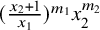
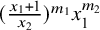
Proof. According to Example 2.14, there are five classes of cluster monomials and we prove that they are log-concave one by one:
-
(1) It is direct that the cluster monomials
$x_1^{m_1}x_2^{m_2}$
are log-concave. -
(2) Since
$(x_2+1)^{m_1}$
is log-concave, by Remark 2.19, we get that
$(\frac {x_2+1}{x_1})^{m_1}x_2^{m_2}$
is log-concave. -
(3) In order to prove that
$(\frac {x_2+1}{x_1})^{m_1}(\frac {x_1+x_2+1}{x_1x_2})^{m_2}$
is log-concave, we only need to prove that
$T_{m_1,m_2}=(x_2+1)^{m_1}(x_1+x_2+1)^{m_2}$
is log-concave. Note that
$$ \begin{align*} T_{m_1,m_2} =\ &{}(x_2+1)^{m_1}\sum\limits_{i=0}^{m_2}C_{m_2}^ix_1^{m_2-i}\left(x_2+1\right)^i\notag \\ =&{}\sum\limits_{i=0}^{m_2}C_{m_2}^ix_1^{m_2-i}(x_2+1)^{m_1+i}\notag \\ =&{} \sum\limits_{i=0}^{m_2}C_{m_2}^ix_1^{m_2-i}\left(\sum\limits_{j=0}^{m_1+i}C_{m_1+i}^jx_2^j\right) \notag \\ =&{}\sum\limits_{i=0}^{m_2}\sum\limits_{j=0}^{m_1+i}C_{m_2}^iC_{m_1+i}^jx_1^{m_2-i}x_2^j\notag. \end{align*} $$
Let
$k=m_2-i$
and
$l=j$
. Then we have (44)
$$ \begin{align} \sum\limits_{i=0}^{m_2}\sum\limits_{j=0}^{m_1+i}C_{m_2}^iC_{m_1+i}^jx_1^{m_2-i}x_2^j=\sum\limits_{k=0}^{m_2}\sum\limits_{l=0}^{m_1+m_2-k}C_{m_2}^{k}C_{m_1+m_2-k}^lx_1^{k}x_2^{l}. \end{align} $$
Note that for each monomial
$x_1^kx_2^l$
in (44), the corresponding coefficient consists of a single term and we denote it by (45)
$$ \begin{align}a_{k,l}=C_{m_2}^{k}C_{m_1+m_2-k}^l.\end{align} $$
According to Example 2.18 and Lemma 5.2, we conclude that
$$ \begin{align*} a_{k,l}^2&=(C_{m_2}^{k}C_{m_1+m_2-k}^l)^2 \notag \\ &\geq C_{m_2}^{k-1}C_{m_2}^{k+1}C_{m_1+m_2-(k-1)}^lC_{m_1+m_2-(k+1)}^l\notag \\ &= a_{k-1,l}a_{k+1,l.}\notag \end{align*} $$
Similarly, we have
$a_{k,l}^2\geq a_{k,l-1}a_{k,l+1}$
. -
(4) By symmetry, it is similar to the proof of (3).
-
(5) Since
$(x_1+1)^{m_2}$
is log-concave, by Remark 2.19, we get that
$(\frac {x_1+1}{x_2})^{m_1}x_1^{m_2}$
is log-concave.







Therefore, all the cluster monomials of type $A_2$
are log-concave.
$A_2$
are log-concave.
Remark 5.4. By use of the properties of binomial coefficients, we have proved the log-concavity of cluster monomials (theta functions) of type $A_2$
. However, it is quite difficult to deal with the cases of type
$A_2$
. However, it is quite difficult to deal with the cases of type $A_n$
with
$A_n$
with $n\geq 3$
, but we believe it is correct. Hence, we give a conjecture to finish this section.
$n\geq 3$
, but we believe it is correct. Hence, we give a conjecture to finish this section.
Conjecture 5.5. The cluster monomials of type $A_n(n\geq 3)$
are log-concave.
$A_n(n\geq 3)$
are log-concave.
6. Log-concavity of F-polynomials of type
$A_n$

In this section, we recall the notions of C-matrices, G-matrices, and F-polynomials based on [Reference Fomin and Zelevinsky8]. Furthermore, according to [Reference Gyoda11], we give the definitions of f-vectors and F-matrices. We aim to prove the log-concavity of F-polynomials of type $A_n$
with
$A_n$
with $n\geq 2$
.
$n\geq 2$
.
6.1. F-polynomials and f-vectors
Before giving the definition of F-polynomials, we recall two crucial notions of C-matrices and G-matrices as follows.
Definition 6.1 [Reference Fomin and Zelevinsky8, Equation (5.9), Proposition 6.6].
Let $B_0$
be the initial exchange matrix at
$B_0$
be the initial exchange matrix at $t_0$
. Then, the collections of integer square matrices
$t_0$
. Then, the collections of integer square matrices $\big \{C_t^{B_0;t_0}\big \}_{t\in \mathbb {T}_n}$
and
$\big \{C_t^{B_0;t_0}\big \}_{t\in \mathbb {T}_n}$
and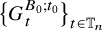 $\big \{G_t^{B_0;t_0}\big \}_{t\in \mathbb {T}_n}$
are recursively defined as follows:
$\big \{G_t^{B_0;t_0}\big \}_{t\in \mathbb {T}_n}$
are recursively defined as follows:
-
(1) (C-matrices) The initial condition is
(46)and for any edge
$$ \begin{align} C^{B_0; t_0}_{t_0}=I_n, \end{align} $$
$t \stackrel {k}{\longleftrightarrow } t^{\prime }$
in
$\mathbb {T}_n$
, the recursion formula is (47)
$$ \begin{align} C^{B_0; t_0}_{t'}=C^{B_0; t_0}_t\big(J_k+[ B_t]^{k \bullet}_+\big)+\big[- C^{B_0; t_0}_t\big]^{\bullet k}_+ B_t. \end{align} $$
-
(2) (G-matrices) The initial condition is
(48)and for any edge
$$ \begin{align} G^{B_0; t_0}_{t_0}=I_n, \end{align} $$
$t \stackrel {k}{\longleftrightarrow } t^{\prime }$
in
$\mathbb {T}_n$
, the recursion formula is (49)
$$ \begin{align} G^{B_0; t_0}_{t'}=G^{B_0; t_0}_t\big(J_k+[ B_t]^{\bullet k}_+\big)-B_0\big[ C^{B_0; t_0}_t\big]^{\bullet k}_+. \end{align} $$


Remark 6.2. By [Reference Fomin and Zelevinsky8, Equation (6.14)], there is a duality between C-matrices and G-matrices:
 $$ \begin{align} B_0C^{B_0; t_0}_t=G^{B_0; t_0}_tB_t. \end{align} $$
Definition 6.3 (Principal coefficients).
A cluster algebra $\mathcal {A}$
is said to have principal coefficients at vertex
$\mathcal {A}$
is said to have principal coefficients at vertex $t_0$
if
$t_0$
if $\mathbb {P}=\text {Trop}(y_1,\dots ,y_n)$
and
$\mathbb {P}=\text {Trop}(y_1,\dots ,y_n)$
and $\mathbf {y}_{t_0}=(y_1,\dots ,y_n)$
.
$\mathbf {y}_{t_0}=(y_1,\dots ,y_n)$
.
When a cluster algebra $\mathcal {A}$
has principal coefficients, we can define the F-polynomial
$\mathcal {A}$
has principal coefficients, we can define the F-polynomial $F^{B_0;t_0}_{i;t}(\mathbf {y})$
as follows:
$F^{B_0;t_0}_{i;t}(\mathbf {y})$
as follows:
 $$ \begin{align} F^{B_0;t_0}_{i;t}(\mathbf{y})=x_{i;t}(x_1,\dots, x_n)|_{x_1=\cdots=x_n=1}=N_{i;t}(1,\dots, 1). \end{align} $$
Denote the maximal degree of $y_j$
in
$y_j$
in $F_{i;t}^{B_0;t_0}(\mathbf {y})$
by
$F_{i;t}^{B_0;t_0}(\mathbf {y})$
by $f_{ji;t}$
. Then, we can define the f-vector
$f_{ji;t}$
. Then, we can define the f-vector $\mathbf {f}_{i;t}^{B_0;t_0}$
and F-matrices
$\mathbf {f}_{i;t}^{B_0;t_0}$
and F-matrices $F_t^{B_0;t_0}$
as follows:
$F_t^{B_0;t_0}$
as follows:
 $$ \begin{align} \mathbf{f}_{i;t}^{B_0;t_0}=\mathbf{f}_{i;t}=\begin{pmatrix}f_{1i;t}\\ \vdots \\ f_{ni;t} \end{pmatrix},\ F_t^{B_0;t_0}=F_t=(\mathbf{f}_{1;t},\dots,\mathbf{f}_{n;t}). \end{align} $$
Definition 6.4 [Reference Fomin and Zelevinsky8, Corollary 6.3].
Let $\mathcal {A}$
be a coefficient-free cluster algebra with the initial exchange matrix
$\mathcal {A}$
be a coefficient-free cluster algebra with the initial exchange matrix $B_0$
. Then, for any
$B_0$
. Then, for any $t \in \mathbb {T}_n$
and
$t \in \mathbb {T}_n$
and $i \in \{1, \dots , n\}$
, we have
$i \in \{1, \dots , n\}$
, we have
 $$ \begin{align} x_{i;t} = \big( \prod_{j=1}^n x_j^{g_{ji;t}} \big)F_{i;t}^{B_0;t_0}(\hat y_1, \dots, \hat y_n), \end{align} $$
where $\hat y_k = \mathop {\prod }\limits _{j=1}^n x_j^{b_{jk}}$
and
$\hat y_k = \mathop {\prod }\limits _{j=1}^n x_j^{b_{jk}}$
and $g_{ji;t}$
is the
$g_{ji;t}$
is the $(j,i)$
-element of
$(j,i)$
-element of $G_t^{B_0;t_0}$
. Formula (53) is usually called the coefficient-free separation formula of
$G_t^{B_0;t_0}$
. Formula (53) is usually called the coefficient-free separation formula of $x_{i;t}$
.
$x_{i;t}$
.
Remark 6.5. By Theorem 4.2 and the separation formula (53), we can directly deduce that the Laurent polynomial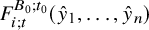 $F_{i;t}^{B_0;t_0}(\hat y_1, \dots , \hat y_n)$
is log-concave with respect to
$F_{i;t}^{B_0;t_0}(\hat y_1, \dots , \hat y_n)$
is log-concave with respect to $x_i$
. However, it cannot directly imply that each F-polynomial
$x_i$
. However, it cannot directly imply that each F-polynomial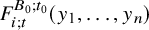 $F_{i;t}^{B_0;t_0}( y_1, \dots , y_n)$
is log-concave with respect to
$F_{i;t}^{B_0;t_0}( y_1, \dots , y_n)$
is log-concave with respect to $y_i$
. In the next section, we aim to prove this fact.
$y_i$
. In the next section, we aim to prove this fact.
Firstly, there is an important relation between f-vectors and d-vectors of cluster algebras of finite type (such as type $A_n$
) as follows.
$A_n$
) as follows.
Theorem 6.6 [Reference Gyoda11, Theorem 1.8].
In a cluster algebra $\mathcal {A}$
of finite type, for any
$\mathcal {A}$
of finite type, for any $i\in \{1,\dots ,n\}$
and
$i\in \{1,\dots ,n\}$
and $t\in \mathbb {T}_n$
, we have
$t\in \mathbb {T}_n$
, we have
 $$ \begin{align} \mathbf{f}_{i;t}=[\mathbf{d}_{i;t}]_+. \end{align} $$
6.2. Geometric realization of d-vectors of type
$A_n$

In this section, we use the geometric realization of d-vectors of type $A_n$
and prove the log-concavity of F-polynomials of type
$A_n$
and prove the log-concavity of F-polynomials of type $A_n$
. Following the geometric realization of cluster algebras of type
$A_n$
. Following the geometric realization of cluster algebras of type $A_n$
in Section 3.1, we let T be the initial triangulation of
$A_n$
in Section 3.1, we let T be the initial triangulation of $(n+3)$
-gon, which corresponds to the initial cluster
$(n+3)$
-gon, which corresponds to the initial cluster $\mathbf {x}=\mathbf {x}_{T}$
.
$\mathbf {x}=\mathbf {x}_{T}$
.
Proposition 6.7 [Reference Fomin, Shapiro and Thurston4, Theorem 8.6].
Let $\mathcal {A}$
be a cluster algebra of type
$\mathcal {A}$
be a cluster algebra of type $A_n$
and
$A_n$
and $x_{\gamma }$
be the cluster variable corresponding to the diagonal
$x_{\gamma }$
be the cluster variable corresponding to the diagonal $\gamma $
, where
$\gamma $
, where $\gamma \notin T$
. Then its corresponding d-vector is
$\gamma \notin T$
. Then its corresponding d-vector is
 $$ \begin{align} \mathbf{d}_\gamma= \begin{pmatrix}d_{1}\\ \vdots \\ d_{n} \end{pmatrix}, \end{align} $$
where $d_{j}$
is the number of intersections between
$d_{j}$
is the number of intersections between $\gamma $
and
$\gamma $
and $T_j$
.
$T_j$
.
Based on the preparations above, we are ready to prove the theorem as follows.
Theorem 6.8. All the F-polynomials of cluster algebras of type $A_n$
are log-concave.
$A_n$
are log-concave.
Proof. There are two possible cases of F-polynomials to be discussed:
-
(1) If the cluster variable
$x_{i;t}$
belongs to the initial cluster
$\mathbf {x}$
, then
$F_{i;t}(y_1,\dots ,y_n)=1$
and it is log-concave immediately. -
(2) If the cluster variable
$x_{i;t}$
does not belong to the initial cluster
$\mathbf {x}$
, then by the geometric realization and Proposition 6.7, we have (56)for any
$$ \begin{align}0\leq d_{ji;t}\leq 1\end{align} $$
$j\in \{1,\dots ,n\}$
. Hence, according to Theorem 6.6, we have (57)for any
$$ \begin{align}0\leq f_{ji;t}\leq 1\end{align} $$
$j\in \{1,\dots ,n\}$
. As a consequence, by the definition of f-vectors, we conclude that
$F_{i;t}(y_1,\dots ,y_n)$
is log-concave.


Example 6.9. The C-matrices, D-matrices (consisting of d-vectors), G-matrices, and F-polynomials of type $A_2$
are as follows (see Table 2). It is direct that the F-polynomials of type
$A_2$
are as follows (see Table 2). It is direct that the F-polynomials of type $A_2$
are log-concave.
$A_2$
are log-concave.
Cluster information of type $A_2$
with principal coefficients
$A_2$
with principal coefficients

Acknowledgements
The authors want to thank the reviewers for their valuable comments and insightful suggestions.
Funding statement
Z.C. is supported by the National Natural Science Foundation of China (Grant No. 124B2003) and China Scholarship Council (Grant No. 202406340022) and Z.S. is supported by the National Natural Science Foundation of China (Grant No. 12471068).


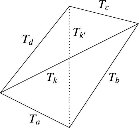
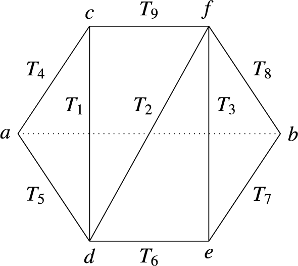


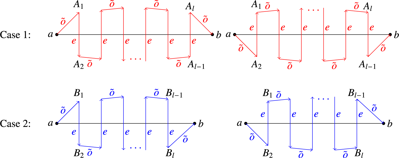
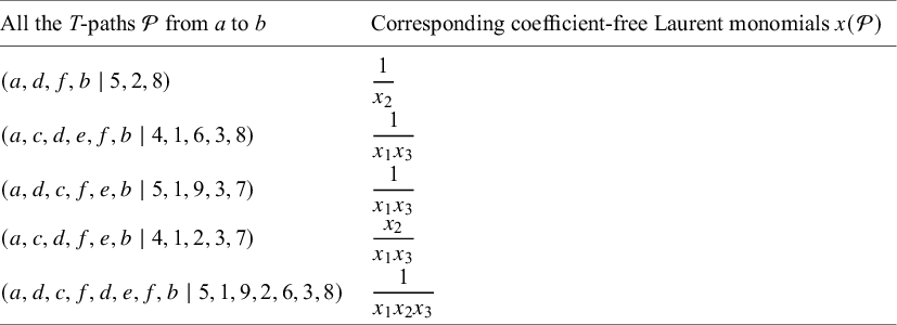

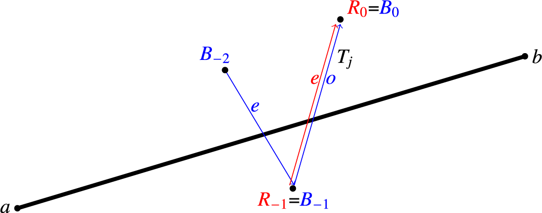

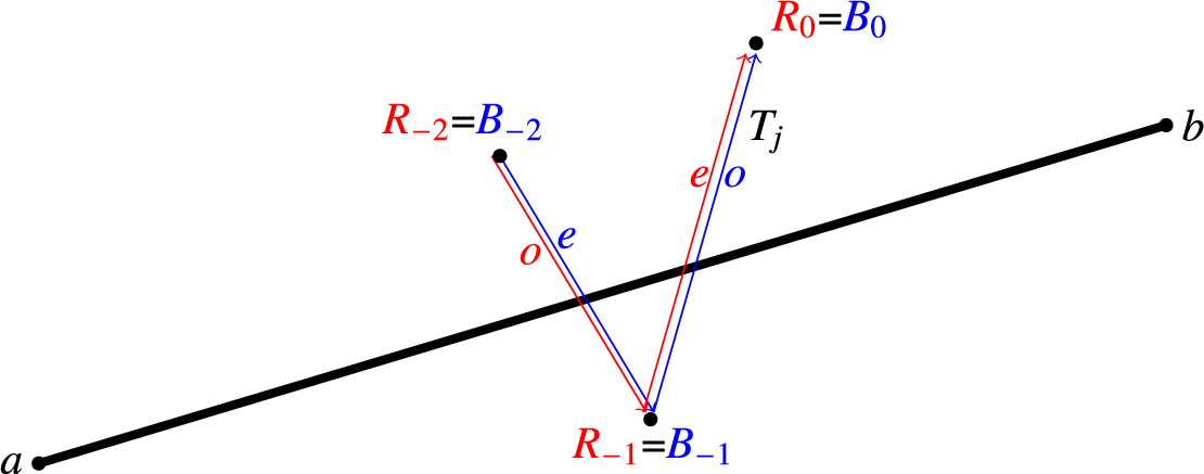


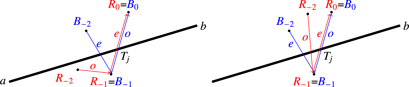


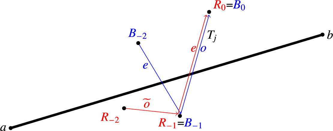


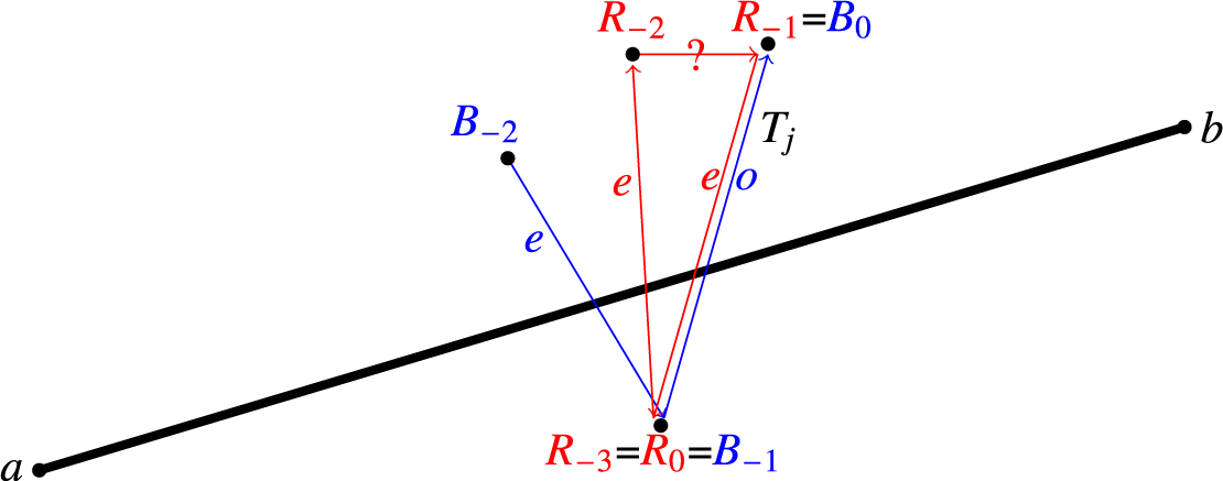


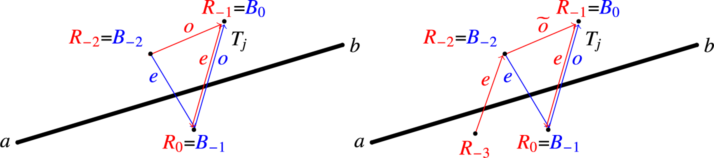


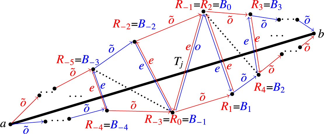


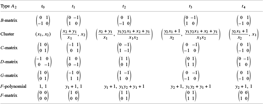


 Open access

