

1 Introduction
Sixty years have passed since the realization of the laser by T. H. Maiman in 1960. The laser is considered to be one of the best inventions of the 20th century and continues to develop in the 21st century. Inventions, combined with social demands and scientific progress, can lead to unexpected new research developments. Human imagination is a wonderful, amazing thing. In 1962, when a 0.01 J short-pulse laser became possible at last, a scientist was convinced that laser fusion could be approached if its output was increased by a factor of 100,000 to 1 kJ, so he visited Maiman and asked him about the possibility, to which Maiman replied with confidence that it would be possible in the near future. This story is very encouraging, when you are thinking about something unexpected.
In 1964, around the time of the beginning of research with short-pulse, high-intensity lasers and the birth of the term ‘laser plasma’, Dawson published a paper discussing the properties and potential applications of laser plasmas[Reference Dawson1]. In the paper, it is described that the high-intensity laser is a simulator of astrophysics and could be used as a tool to study physics related to collisionless shock waves in supernova explosions and solar flares in the laboratory. However, this paper did not provide an immediate impetus for a simulated laser experiment for astrophysics research. At that time, we had no idea about what kind of plasma the laser plasma itself was, and our hands were full simply generating, measuring, and analyzing the plasma produced by an intense laser. In addition, various nonlinear phenomena such as anomalous absorption and parametric instability have been observed in plasmas irradiated by lasers. We have not, however, yet reached the stage of application to fusion energy or astrophysics research, and remain at the level of trying to understand the plasma itself. The application to fusion energy had to wait for the first oil crisis in 1973.
1.1 Laser implosion is still fundamental science
Here, the first author would like to describe his personal history of the proposal of laboratory astrophysics during the time he was heavily involved in hydrodynamic instability in laser implosion for fusion energy research in Institute of Laser Engineering (ILE), Osaka University.
It was 1972 when Prof. C. Yamanaka established the current ILE at Osaka University. He selected laser fusion energy research as the main subject of the new institute. Thanks also to the enthusiasm of the nation because of the energy crisis, the 30-kJ, 12-beam laser facility Gekko-XII was constructed in 1983 to demonstrate the scientific feasibility of laser-driven implosion and fusion neutron production. After a lot of implosion experiments, it became clear that the hydrodynamic instability and turbulent mixing were critical to prevent the spherical implosion of the fusion fuel. The summarizing paper on the fusion performance and the relation to the hydrodynamic instability and mixing was published in 1988[Reference Takabe, Yamanaka, Mima, Yamanaka, Azechi, Miyanaga, Nakatsuka, Jitsuno, Norimatsu, Takagi, Nishimura, Nakai, Yabe, Sasaki, Yoshida, Nishihara, Kato, Izawa, Yamanaka and Nakai2].
Accidentally, it was at the time that the series of workshops focusing on fundamental aspects of turbulent mixing in matter acceleration in both compressible and incompressible fluids started in 1988[3]. The International Workshops on the Physics of Compressible Turbulent Mixing has been bi-annually organized internationally. This workshop was initiated to aid in understanding the hydrodynamic mixing demonstrated experimentally[Reference Read4] and computationally[Reference Youngs5] in 1984. The hydrodynamic instabilities and resulting turbulent mixing in laser implosion dynamics are still full of open questions as fundamental physics and we need more time for research to control the laser-driven implosion hydrodynamics.
During the first author’s undergraduate course, the first oil shock happened, which motivated him to become a researcher of laser fusion energy. As a graduate student, he started theoretical research of the Rayleigh–Taylor instability at the ablation front, but could not solve it theoretically. Fortunately, he had a chance to challenge this problem with computational methods in the USA. After publishing two papers on the numerical solution and scaling formula[Reference Takabe6, Reference Takabe, Mima, Montierth and Morse7], he was deeply concerned about the hydrodynamic instability and turbulent mixing of compressible fluids in laser-driven implosion.
One day, he was invited by a famous astrophysicist to give a seminar talk on laser fusion research. It was very impressive that the professor appreciated our research into challenging the hydrodynamic instability of implosion; however, he mentioned that ‘there are many challenging topics in astrophysics even with the assumption of one-dimensional geometry, so we have no time to get into such multidimensional problems in this universe’. Of course, the first author was disappointed to hear that, but a young faculty member Dr. Nomoto in his group showed a strong interest in his study of hydrodynamic instability. Dr. Nomoto is a specialist of the ignition scenario of supernovae and studied the case of Type-Ia supernova explosions, which are thermonuclear explosion of a white dwarf (WD) in a binary system, when the mass of the WD becomes Chandrasekar mass (1.4 solar masses). He mentioned to the first author that the ignition is not always at the center of the WD and even the surface starts to ignite the thermonuclear burning wave. The multidimensional hydrodynamics in the gravitational force (inertial force in laser fusion) is essential to studying the physics of supernova ignition.
It is surprising that this communication was done just before the SN1987A explosion was observed. This was the first supernova explosion to be seen with the naked eye in the last 400 years, since the Tycho supernova in 1572. This was a Type II supernova where the explosion is driven by gravitational collapse in the massive star with a mass of more than 8–10 solar masses. After a half year from the observation, the first author received a phone call from Dr. Nomoto saying that ‘Takabe-san, the experiment by God has been done to let us know that supernova explosion is not spherically symmetric and the X-ray observation suggests the turbulent mixing is driven in the explosion phenomenon’.
1.2 The same physics controls the small implosion and huge explosion
This supernova named SN1987A, the explosion of which was observed in the southern hemisphere (distance is 160,000 light years) on 23 February 1987, taught us that the study of fluid instability is not only a subject for laser fusion, but also key to supernova explosion physics[Reference Hachisu, Matsuda, Nomoto and Shigeyama8]. Supernova explosions are the most spectacular phenomenon in the universe, where elements heavier than helium are nucleo-synthesized before and during the explosion and eventually scattered into space by the supernova explosion. Billions of years later, ejected material of this type became the source of the formation of the Earth and the birth of life and humans. This is a magnificent thought. The story of the deep involvement of fluid instabilities in the determination of the scale of supernova explosions has given us confidence that laser fusion researchers are studying not only the world of implosion plasmas in 1 mm space, but also explosions of tens of thousands of kilometers of space in the universe. This fact has reminded us of the importance of having eyes wide open to the physics.
It is very clear that the urgent issue to be solved in two different fields in laser implosion and supernova explosion are the same by just showing the two data: experimental neutron yield in laser implosion and observational X-ray intensity time evolution from SN1987A explosion. In Figure 1, the experimental deuterium–tritium (DT) fusion neutron yield per input laser energy of 10 kJ is plotted as a function of the spherical glass shell thickness with DT fusion fuel gas inside. The experimental data are plotted with the solid circles, while corresponding one-dimensional implosion simulation data are plotted with  $\boxplus$ marks[Reference Takabe, Yamanaka, Mima, Yamanaka, Azechi, Miyanaga, Nakatsuka, Jitsuno, Norimatsu, Takagi, Nishimura, Nakai, Yabe, Sasaki, Yoshida, Nishihara, Kato, Izawa, Yamanaka and Nakai2]. It is seen that even at the best agreement to the experimental yield, the experimental yield is half of the one-dimensional yield. The discrepancy increases as the aspect ratio decreases, namely through the use of a thicker glass shell. This discrepancy is found to be because of the Rayleigh–Taylor instability at the final implosion phase. Including a turbulent mixing model in the one-dimensional implosion code, we could reproduce the experimental yield numerically as shown with the three following marks. This is our understanding of the fatal problem for laser fusion at the stage of the mid-1980s.
The experimental neutron yield of deuterium–tritium (DT) fuel implosion per 10 kJ laser energy is indicated with solid circles. The neutron yields obtained with one-dimensional implosion simulations are shown with  $\boxplus$ marks, where the values are the corresponding neutron yield for all solid circle experimental data. The other three data sources are obtained by including the $k-\unicode{x3b5}$ type turbulent mixing model in the one-dimensional implosion code in the final stagnation phase. This indicates how the turbulent mixing is serious in the final stagnation phase through which the kinetic energy of imploding fluid is converted into the thermal energy of DT plasma[Reference Takabe, Yamanaka, Mima, Yamanaka, Azechi, Miyanaga, Nakatsuka, Jitsuno, Norimatsu, Takagi, Nishimura, Nakai, Yabe, Sasaki, Yoshida, Nishihara, Kato, Izawa, Yamanaka and Nakai2].

In Figure 2, the observation data of X-ray emission from SN1987A are plotted with solid circles with error bars as a function of days. The data are taken by Japanese X-ray satellite GINGA[Reference Inoue, Hayashida, Itoh, Kondo, Mitsuda, Takeshima, Yoshida, Tanaka and Publ9]. The hard X-ray of 16–28 keV stems from the nuclear decay of  ${}^{56}$Ni predicted to be generated near the center of SN1987A. As the optical thickness of the outer layer is thick and decreases as the matter expands, it is predicted to take about 1 year to be observed in the one-dimensional explosion simulation as plotted with the dashed line. However, GINGA satellite began to observe the X-ray about 100 days after the explosion. Scientists considered that the explosion is hydrodynamically unstable and the mixing of inside and outside materials conveys the central
  ${}^{56}$Ni outer region relatively optically thin. Therefore, the effect of Rayleigh–Taylor instability is modeled in one-dimensional code to see the X-ray signal and it was found that the uniform mixing plus clumpy spike–bubble model can explain the data indicated as the solid line, not by uniform mixing.
The time evolution of hard X-ray emission flux as a function of the day after the supernova SN1987A explosion. The observation data are plotted with solid circles with error bars. The time history predicted by one-dimensional supernova simulation is shown with a dashed line. It is clear that the signals came earlier by 150 days than the prediction. Such a long-time appearance of the X-ray was modeled with artificial uniform mixing and mixing with a clumpy structure: long-wavelength deformation. It is concluded that the clumpy mixing could explain the explosion hydrodynamics. This is the serious start for supernova physics to include three-dimensional effect as a standard model. It is noted that the hard X-rays at 18–26 keV are generated after the Comptonization of the gamma-rays generated by nuclear decay of created Ni in the central region of the supernova[Reference Inoue, Hayashida, Itoh, Kondo, Mitsuda, Takeshima, Yoshida, Tanaka and Publ9].

Research collaboration started in the year of the SN1987A explosion because of such clear similarity in different time–space scales and the difference between implosion and explosion. The collaboration was mainly among theory and computation. During such collaboration, the first author found that computer simulation scientists were not convinced about the appropriateness of their basic equations and numerical modeling. The astrophysics is difficult to study experimentally and there are no ways to compare simulations with any kind of model experimental data. So-called verification and validation of sophisticated codes are impossible in astrophysics and there is no confidence in the simulation results.
Having discovered this fact, we discussed a possibility to perform a variety of model experiments with intense lasers. It was initiated by the discussion to use a laser facility to provide the data for the verification and validation of the astrophysical codes. However, this initial small idea has grown to the proposal of a new research field of astrophysics, namely laboratory astrophysics. It should be noted that the progress from a premature idea of code validation to the new method of astrophysics study is thanks to the many complaints from the laser-plasma scientists. What they complained about was that they did not want to be slaves of astrophysics, working just to provide the data for verification. They argued that if we do something, it should be a new creative action in the laser plasma community. That is, we have to aim at finding physics in astrophysical phenomena. This was the start of real laboratory astrophysics research.
In line with the above, the first author has listened to lectures on supernova physics and held discussions directly with many astrophysicists. He found that many related physics are the same as those in laser plasma, and the only difference is the scale of the space–time. Then, remembering a variety of self-similar solutions especially in compressible hydrodynamic phenomena, it is the starting point to make a physics simple to try to find the key nondimensional parameters to use high-intensity lasers to study astrophysics.
1.3 Laboratory astrophysics aims at the prediction of new physics
The first author (H. T.) usually started his talks with the picture shown in Figure 3. Of course, it is initiated as the testbed experiment for the validation of simulation codes applied to astrophysics. However, even in the process of comparing model experimental data with astrophysical simulation, we can find new physics not modeled in the astrophysical simulation codes. This is also a new finding of laser plasma. The third step shown in Figure 3 is ‘challenge’. A huge diversity of fundamental plasma physics can be found in the universe, so we should not restrict our attention to plasmas in the laboratory. For academic development in plasma physics, we need to always prepare young people with advanced and challenging physics tasks. There is no way to avoid the challenge of finding physics in the universe, which is full of plasma physics. Finally, when laboratory astrophysics reaches maturity, we hope we can predict new physics that are beyond what has previously been imagined.
The four steps of laboratory astrophysics are described. The physics in both the laser plasma and astrophysical plasma is connected in general with help of computer simulation.

In 1998 in such emerging phase, the first author was given a chance to present his personal thoughts on why I wish to move to academic, fundamental research like laboratory astrophysics from a purpose-oriented fusion energy research at a big conference in Prague. The talk was given in front of about 1000 researchers mainly working in magnetic and laser fusion energy. The presentation is reproduced in the Appendix posted at the end of this paper consisting of one example of a history of change from purpose-oriented to fundamental research.
There are two points of view linking laser-generated plasma and astrophysics, that is, sameness and similarity. One is that the physics are identical, and the other is that the physical phenomena or dynamics are similar in nondimensional time and space. Examples are as follows.
(1) Sameness of physics:
(a) equation of state; (b) opacity; (c) nuclear reaction.
(2) Physical similarity:
(a) dynamical phenomena of compressible fluids; (b) nonequilibrium atomic processes; (c) radiant energy transport
Class (1) is easy to understand. For example, a laser fusion implosion experiment has achieved a plasma state comparable to the temperature and density of the Sun’s interior. The thermodynamic properties of such plasma are determined by temperature and density. The thermodynamic properties of astronomical objects can be studied in detail by generating small pieces with a high-intensity laser and studying them in the laboratory. This is also the case of radiation properties such as emission and absorption spectra of X-rays.
Class (2) is an attempt to elucidate various physics of fluid phenomena, atomic processes and so on by transforming time and space scales to the power of 10–20 (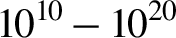 ${10}^{10}-{10}^{20}$) on the basis of the similarity law. It is widely possible to reduce the phenomena to the time scale of the density ratio (
 ${\sim}{10}^{20}$) from that in astrophysics to the phenomena in nanoseconds in the laboratory. Therefore, as an example, the author considered the hydrodynamic similarity between laser implosion and supernova explosions to clarify the physics of hydrodynamic instability of the SN1987A explosion[Reference Takabe10]. The origin of fluid instability and convective motion during explosions, which had been a major issue in studying SN1987A, was discussed with the knowledge of laser implosion. At the same time, such activity is beneficial for both research fields and a laser fusion guy started a collaboration for researching the supernova physics[Reference Nomoto, Iwamoto, Shigeyama and Takabe11]. We have also published a proposal of this concept with the title of article ‘Laboratory astrophysics with intense lasers’ in monthly journal of The Physical Society of Japan, one figure of which was used as the cover of the journal as shown in Figure 4[Reference Takabe and Nomoto12]. In the last 30 years, multidimensional simulation of core-collapse supernova explosion has been studied intensively and recent three-dimensional simulation gives explosion scenario with hydrodynamic instability. A snapshot of three-dimensional hydro-simulation is shown in Figure 5[Reference Burrows, Radice and Vartanyan13].
The cover of the journal ‘BUTSURI’ in Japanese, indicating the image of laboratory astrophysics. The top-left figure is a two-dimensional hydrodynamic simulation of the SN1087A explosion with the initial condition of the most plausible progenitor. Hydrodynamic instability and mixing are suggested. The top-right and bottom are the density and temperature profiles from two-dimensional hydrodynamic simulation near the time of maximum compression of the final stage of the implosion experiment with a Gekko XII laser system.

Three-dimensional simulation of supernova explosion. The green surface is the surface of a shock wave propagating outward[Reference Burrows, Radice and Vartanyan13].

1.4 Start of model experiments and many future topics
When SN1987A inspired the idea of laboratory astrophysics, B. Remington initiated experimental activity at Lawrence Livermore National Laboratory (LLNL). Therefore, we first reviewed possible laboratory astrophysics experiments[Reference Remington14, Reference Remington, Drake, Takabe and Arnett15]. At the same time, the first author summarized the conceivable, expected laboratory astrophysics experiments in a review paper from the angles of sameness, similarity, and resemblance[Reference Takabe16]. Twenty years ago, the first author explained the following themes. They were mainly theoretical proposals.
(1) Hydrodynamics and shocks:
equation of state; strong shock–matter interactions.
(2) Hydrodynamic instabilities:
laser implosion and SN1987A; instabilities in three phases in Type II supernova explosion; hydrodynamic instability in Type Ia supernovae; ultraviolet (UV) radiation-driven Rayleigh–Taylor instability causing pillars of Eagle Nebula.
(3) Atomic physics and X-ray transport:
opacity and opacity experiment; hydrodynamics of supernova remnants; nonlocal thermodynamic equilibrium atomic processes in supernova remnants; Vishiniac instability; stellar jets; photoionized plasmas.
(4) Laser-produced relativistic plasmas:
relativistic electron production; a variety of physics triggered by relativistism; positron creation by ultra-intense lasers; model experiments with relativistic electron–positron plasmas.
Most of such topics have been studied experimentally as laboratory astrophysics research and its community has become widespread in the last 20 years. In the following, we would like to revisit the above three papers and briefly review the progress by citing references, especially experimental research, over the past 20 years. At the same time, we would like to explain the topics that were not conceived of at that time but have been actively studied by the community in the last 20 years. It is also important to point out that many review papers have been published in the last two decades by focusing on a variety of physics accomplished experimentally and predicted theoretically, reflecting the growth of the research community.
It is surprising to look at the rapid progress of this research in the last two decades. To commemorate the 60th anniversary of the birth of the laser, we have tried to briefly review the 10 subjects where outstanding progress of experimental results has been reported in the last two decades. It should be noted that some of them have been awarded prizes by the American Physical Society (APS) to recognize a particular recent outstanding achievement in plasma physics research.
1.5 APS Dawson awards to laboratory astrophysics related topics
John Dawson Award for Excellence in Plasma Physics Research[17]
(A) Hideaki Takabe, Hye-Sook Park, Dmitri Ryutov, Steven Ross, Frederico Fiuza, Youichi Sakawa, Anatoly Spitkovsky, Christoph Niemann, William Fox, R. Paul Drake, Gianluca Gregori (2020)
‘For generating Weibel-mediated collisionless shocks in the laboratory, impacting a broad range of energetic astrophysical scenarios, plasma physics, and experiments using high energy and high power lasers conducted at basic plasma science facilities’.
(B) Alexander Schekochihin, Donald Lamb, Dustin Froula, Gianluca Gregori, Petros Tzeferacos (2019)
‘For innovative experiments that demonstrate turbulent dynamo in the laboratory, establishing laboratory experiments as a component in the study of turbulent magnetized plasmas, and opening a new path to laboratory investigations of other astrophysical processes’.
(C) Andrew James MacKinnon, Chikang Li, Fredrick H. Seguin, Marco Borghesi, Oswald Willi, Richard D. Petrasso (2017)
‘For pioneering use of proton radiography to reveal new aspects of flows, instabilities, and fields in high-energy-density plasmas’.
(D) James Bailey (2016)
‘For extraordinarily thorough laboratory opacity measurements of plasmas at realistic stellar interior conditions that directly resolve outstanding questions about solar structure, identify new theoretical challenges, and propel a new generation of precision high energy density experiments of direct astrophysical relevance’.
(E) Bob Nagler, Hyun-Kyung Chung, Justin Wark, Orlando Ciricosta, Philip Heimann, Richard W. Lee, Roger Falcone, Sam M. Vinko (2015)
‘For creative and novel use of the hard X-ray free electron laser to isochorically create high density plasmas and accurately measure the ionization potential depression, and for new theory that addresses discrepancies with long standing models and provides stimulus for continued developments’.
The readers may be aware that the above awardees (A)–(E) have played key roles in the advancement of laboratory astrophysics as an attractive subject with maturity and diversity. For example, the recipients in (C) have developed the technology of proton radiography with precision resolution. Without this measurement technology the Weibel instability and magnetic turbulence in the work of recipients in (A) cannot be measured to discuss the physics of collisionless shocks. The recipients in (E) gave the answer to a long-standing question in astrophysics. This has clarified experimentally that the commonly used theory of ionization potential depression in high-density plasma in astrophysics, the Stewart–Pyatt model, is different from the experimental data with the ionization and recombination dynamics of aluminum solid heated by X-FEL.
1.6 Ten topics to be reviewed
In Section 2, the first author briefly reviewed the 10 topics focusing on recent experimental accomplishment and theoretical status. In the 10 topics, we have focused on laboratory astrophysics subjects regarding collisionless plasmas produced by lasers, mainly on magnetic field generation and turbulence. We have also reviewed the physics of high-energy-density plasmas regarding the topics of equation of state (EOS), atomic physics, and hydrodynamic phenomena using high-pressure generated by intense lasers. It should be noted that a special issue of recent activity on laboratory astrophysics was also published in this journal as the ‘HPLSE special issue on laboratory astrophysics’[Reference Suzuki-Vidal, Lebedev, Ciardi, Pickworth, Rodriguez, Gil, Espinosa, Hartigan, Swadling, Skidmore, Hall, Bennett, Bland, Burdiak, de Grouchy, Music, Suttle, Hansen and Frank18].
The subjects of the 10 topics are as follows:
(1) magnetic reconnection experiments;
(2) magnetic turbulence experiments;
(3) collisionless shock mediated by Weibel instability and magnetic turbulence;
(4) modeling cosmic-ray generation stemming from stochastic acceleration by nonlinearity of direct interaction between relativistic laser and charged particles;
(5) electron–positron plasma generation by ultra-intense lasers;
(6) EOS experiment of high-energy-density plasmas compressed by shocks from lasers;
(7) opacity measurement of hot dense plasmas produced by lasers;
(8) photoionized plasma experiment modeling blackhole binary systems;
(9) blast waves generated by astrophysical explosions;
(10) hydrodynamic instability and the physics of turbulent mixing.
In Section 3, the second author (Y. K.) wrote a review of the present status of modeling cosmic-ray acceleration, which is a challenging subject even as laboratory astrophysics. Nonthermal energetic particles or cosmic rays are ubiquitous in the universe. The diffusive shock acceleration (DSA) and the first-order Fermi acceleration are considered as standard theories for the acceleration of galactic cosmic rays; however, the origins of extragalactic cosmic rays are not well understood. A possible mechanism considered to be operative in extreme astrophysical conditions is wakefield acceleration of cosmic rays. In Section 3, we review the wakefield acceleration in astrophysical context and discuss possible verifications in laboratories.
Section 4 is devoted to a brief summary and outlook on laboratory cosmology.
2 Brief review of the 10 topics in recent research on laboratory astrophysics
The 10 topics briefly reviewed here can be roughly divided into 2 categories: collisionless plasma; and collisional plasma or plasma hydrodynamics. The former is rather new topics and magnetic fields play an important role in many cases. The collisionless plasma physics is more complicated because of coupling between charged particles and electric and magnetic fields. However, this diversity is essential in astrophysics and the challenge of collisionless plasma in astrophysics is becoming more attractive as academic research into fundamental plasma physics. In the present paper, focusing on the recent accomplishment with a variety of lasers, mostly experimental results are reviewed. It is also noted that the success of such experiments is thanks to the rapid progress of diagnostic methods. Higher resolution of time and space has made it possible to study, for example, turbulent spectra of magnetic fields and time evolution of fine spectra from ionizing and recombining plasmas. This is also true for the velocity interferometer system for the reflector (VISAR) in the EOS experiment in high-energy-density physics (HEDP).
It should be noted that the authors have no space to describe the historical progress of each topic and focus instead on the most recent accomplishments. Therefore, we do not refer to the papers in which the original idea or fist experiment of each topic has been reported. The readers are recommended to review the references to investigate the history of each topic if they are interested. We hope the readers can obtain their own personalized history by reading many papers in the references.
2.1 Magnetic reconnection experiments
The self-generated magnetic field in laser plasma has been studied from 1970s and strong magnetic fields of the order of megagauss (100 T) have been reported[Reference Stamper19]. In the last decade, this magnetic field has been used to study the physics of magnetic reconnection by many groups. Particle acceleration induced by magnetic reconnection is important for producing the nonthermal particles associated with explosive phenomena such as solar flares, pulsar wind nebulae, and jets from active galactic nuclei (AGN). Laboratory experiments have played an important role in the study of the detailed microphysics of magnetic reconnection and the dominant particle acceleration mechanisms[Reference Yamada, Yoo, Jara-Almonte, Ji, Kulsrud and Myers20]. In particular, the well-designed experiment on electromagnetic fluctuations during fast reconnection was reported[Reference Ji, Terry, Yamada, Kulsrud, Kuritsyn and Ren21] and clearly showed that the turbulent level of the field fluctuation is inversely proportional to the reconnection time. This evidence from magnetically confined plasma in the laboratory is critical to explaining many observation data from solar flares, the scale of which is huge whereas the reconnection time is many orders of magnitude shorter than the reconnection time resulting from the classical collisional process. So-called anomalous resistivity is one of the key issues in magnetic reconnection physics.
In the last decade, magnetic reconnection has been studied with intense lasers by use of its dynamical effect, namely, reconnection driven by plasma flows is easily reproduced. Most of the cases are focused on the magnetic reconnection in high-beta plasmas, which is very hard to set up in magnetized plasma in the laboratory. As the magnetic reconnection is the physical process that charged particles gain kinetic energy through the decrease of total magnetic energy in the reconnecting system, the acceleration process is not as effective in high-beta plasma in general. It is, therefore, important to clearly identify what unique and original physics we can investigate in laser-driven magnetic reconnection compared with the magnetically confined plasma reconnection experiments.
In studying magnetic field production and evolution in plasmas, it is usual to start with the Faraday induction law:
 \begin{align}\nabla \times \overrightarrow{E}=-\frac{\partial \overrightarrow{B}}{\partial t}.\end{align}
 Equation (1) indicates that the appearance of the electric field by charged particle motion induces the magnetic field. Therefore, it is necessary to consider the equation of motion of electrons and ions. As electron mobility is much larger than ion mobility, force balance of the electron fluid is approximately satisfied. Taking account of the ion fluid motion with velocity  $v$, it is easy to obtain the following equation from Equation (1):
 \begin{align}\frac{\partial \overrightarrow{B}}{\partial t}&=\nabla \times \left(\overrightarrow{v}\times \overrightarrow{B}\right)-\nabla \times \left(\frac{\nabla \times \overrightarrow{B}}{\mu_0{\sigma}_{\mathrm{e}\mathrm{i}}}\right)\notag\\&\quad{}-\nabla \times \left(\frac{\overrightarrow{j}\times \overrightarrow{B}}{en}\right)-\frac{\nabla n\times \nabla {P}_{\mathrm{e}}}{en^2}.\end{align}
Note that this is directly related to the vortex equation shown later in Equation (9) in Section 2.10. The last term in Equation (2) is the source term of the magnetic field and is called the Biermann battery effect. The electron vortex motion generates negative current in the form of a ring in the vortex. This current generates the magnetic field.
Once the magnetic field is generated, it can be amplified by the dynamo effect given as the first term on the right-hand side in Equation (2). The velocity in Equation (2) is the flow velocity of plasma fluid, namely ion fluid. When the ion motion is perpendicular to the magnetic field, the fluid motion stretches the magnetic field against the tension, consequently converting fluid kinetic energy to the magnetic field. This is the well-known source of the strong magnetic field of the Sun. Note that the vortex formation in neutral hydrodynamics means the generation of magnetic field in plasmas. Therefore, Rayleigh–Taylor and Richtmyer–Meshkov instabilities always accompany magnetic field in high-temperature plasmas.
A magnetic reconnection experiment was proposed and performed by use of the B-field generated via the Biermann battery effect[Reference Nilson, Willingale, Kaluza, Kamperidis, Minardi, Wei, Fernandes, Notley, Bandyopadhyay, Sherlock, Kingham, Tatarakis, Najmudin, Rozmus, Evans, Haines, Dangor and Krushelnick22]. Two laser beams are focused in close on a planar solid target to generate magnetic field as in Figure 6[Reference Nilson, Willingale, Kaluza, Kamperidis, Minardi, Wei, Fernandes, Notley, Bandyopadhyay, Sherlock, Kingham, Tatarakis, Najmudin, Rozmus, Evans, Haines, Dangor and Krushelnick22]. Simultaneous optical probing and proton grid imaging reveal two high-velocity, collimated outflowing jets in the target normal direction and 0.7–1.3 MG magnetic fields at the focal spot edges. Many experiments were conducted following Ref. [Reference Nilson, Willingale, Kaluza, Kamperidis, Minardi, Wei, Fernandes, Notley, Bandyopadhyay, Sherlock, Kingham, Tatarakis, Najmudin, Rozmus, Evans, Haines, Dangor and Krushelnick22]. Such laser reconnection experiments have recently been reviewed, for example, in Ref. [Reference Zhong, Yuan, Han, Sun and Ping23]. Proton backlight diagnostics now provide the special distribution of magnetic fields. The time evolutions of proton image and magnetic field are shown in Figure 7[Reference Palmer, Campbell, Ma, Antonelli, Bott, Gregori, Halliday, Katzir, Kordell, Krushelnick, Lebedev, Montgomery, Notley, Carroll, Ridgers, Schekochihin, Streeter, Thomas, Tubman, Woolsey and Willingale24].
Two lasers are irradiated to generate two magnetic fields to drive magnetic reconnection[Reference Nilson, Willingale, Kaluza, Kamperidis, Minardi, Wei, Fernandes, Notley, Bandyopadhyay, Sherlock, Kingham, Tatarakis, Najmudin, Rozmus, Evans, Haines, Dangor and Krushelnick22].

Proton backlight images and reconstructed magnetic field structures[Reference Palmer, Campbell, Ma, Antonelli, Bott, Gregori, Halliday, Katzir, Kordell, Krushelnick, Lebedev, Montgomery, Notley, Carroll, Ridgers, Schekochihin, Streeter, Thomas, Tubman, Woolsey and Willingale24].

The two magnetic fields expand because of plasma expansion and collide with each other to start magnetic reconnection at the central line. Thus, this is pressure-driven magnetic reconnection and the colliding velocity is of the order of sound velocity. The reconnection induces electric field in the target normal direction to accelerate particles. Integration of Equation (1) over an area of the target normal plane gives roughly the induced electric field  $E$. The magnetic reconnection reduces the total magnetic flux to generate the electric field. This electric field accelerates electrons and ions and they are called nonthermal particles. By a simple dimensional analysis we can give a simple relation of the non-thermal particle energy
  ${E}_{\mathrm{nt}}$:
 \begin{align}{E}_{\mathrm{nt}}= qEL=3\times \frac{L}{1\;\mathrm{mm}}\frac{B}{1\;\mathrm{T}}\frac{V_{\mathrm{R}}}{c}\kern1em \left[\mathrm{MeV}\right],\end{align}
where  $E$ is the induced electric field,
  $L$ is the acceleration distance and
  ${V}_{\mathrm{R}}$ is the reconnection velocity. It looks easy to accelerate electrons to relativistic energy, because we have
  $B>100$ T and
  $L\sim 1$ mm, but the problem is the reconnection velocity
  ${V}_{\mathrm{R}}\left(\ll c\right)$ in most experiments. The relativistic magnetic reconnection with
  ${V}_{\mathrm{R}}/c\sim 1$ and
 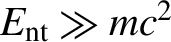 ${E}_{\mathrm{nt}}\gg {mc}^2$ is most cases in astrophysics. Note that regardless of any acceleration mechanics, Equation (3) for
 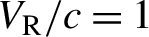 ${V}_{\mathrm{R}}/c=1$ is a measure of astrophysical objects of cosmic-ray acceleration and it is called a Hillas diagram[Reference Hillas25].
Through fully kinetic particle-in-cell (PIC) simulations, the acceleration mechanisms in experiments with colliding magnetized laser-produced plasmas were studied in two-dimensional geometry by focusing the physics of particle acceleration[Reference Fox, Park, Deng, Fiksel, Spitkovsky and Bhattacharjee26]. The simulations observe three phases of particle acceleration, Fermi acceleration in the initially converging magnetized plumes, and X-line acceleration during reconnection and further energization in contracting plasmoids. The Fermi acceleration is first order and electrons go back-and-forth in the reconnection region by magnetic field. PIC simulation in three-dimensional geometry has been performed to demonstrate particle acceleration in laser reconnection experiments[Reference Totorica, Abel and Fiuza27]. The same kind of acceleration physics has been found as in the previous case. The many particle trajectories and their energies are plotted in Figure 8. Most of the particles coming from the bottom are accelerated in the narrow reconnection region and ejected to the top with high energy (red color).
Result of a PIC simulation of laser-driven magnetic reconnection phenomenon. The trajectories of electrons accelerated in the reconnection zone are plotted with color, where the red shows higher energy of accelerated electrons[Reference Totorica, Abel and Fiuza27].

Relativistic-electron-driven magnetic reconnection was demonstrated with the OMEGA-EP laser[Reference Raymond, Dong, McKelvey, Zulick, Alexander, Bhattacharjee, Campbell, Chen, Chvykov, Del Rio, Fitzsimmons, Fox, Hou, Maksimchuk, Mileham, Nees, Nilson, Stoeckl, Thomas, Wei, Yanovsky, Krushelnick and Willingale28]. Relativistic electron acceleration is observed by increasing the reconnection velocity  ${V}_{\mathrm{R}}/c\sim 1$ in Equation (3) by use of ultra-intense lasers (
 ${>}{10}^{18}$ W/cm
 ${}^2$). An increase of nonthermal electrons near 10 MeV is reported. In recent experiment with Gekko and a micro-coil, on the other hand, relativistic reconnection was demonstrated by increasing
  $B$ in Equation (3) with the coil[Reference Law, Abe, Morace, Arikawa, Sakata, Lee, Matsuo, Morita, Ochiai, Liu, Yogo, Okamoto, Golovin, Ehret, Ozaki, Nakai, Sentoku, Santos, D’Humières, Korneev and Fujioka29]. Although a laser intensity of
  ${10}^{14}$–
 ${10}^{16}$ W/cm
 ${}^2$ was used, the well-designed coil generates a magnetic field of 3000 T. It is reported that power-law energy spectra are observed for both protons and electrons in the near-relativistic region.
The electron dynamics has been considered to be crucial to the triggering mechanism of magnetic reconnections. Recent space missions have revealed this with in situ observations. However, it is highly challenging to observe global imaging of magnetic reconnections in space plasmas. In contrast, in astrophysical plasmas it is difficult to obtain the electron-scale microscopic data although global imaging with a telescope is common. Laboratory astrophysics allows us to simultaneously obtain local and global information of magnetic reconnections. We have investigated magnetic reconnections driven by electron dynamics in laser-produced plasmas. We apply a weak external magnetic field, where the electrons are magnetized but the ions are not, that is, only electrons are directly coupled with the magnetic field[Reference Kuramitsu, Moritaka, Sakawa, Morita, Sano, Koenig, Gregory, Woolsey, Tomita, Takabe, Liu, Chen, Matsukiyo and Hoshino30]. The plasmoid and cusp propagating at the electron Alfvén velocity are measured with global imaging, which strongly indicate the magnetic reconnection driven by electron dynamics[Reference Kuramitsu, Moritaka, Sakawa, Morita, Sano, Koenig, Gregory, Woolsey, Tomita, Takabe, Liu, Chen, Matsukiyo and Hoshino30].
Recently, the first local observations of magnetic reconnection driven by electron dynamics have been reported in addition to global observations in laser-produced plasmas[Reference Sakai31]. Collective Thomson scattering measurement provides the local velocities of electrons and ions. It shows the pure electron outflow is not accompanied by ion motion. At the same time, the magnetic induction probe showed the local magnetic field inversion corresponding to the plasmoid propagation. The wavelet analysis of the local magnetic field shows the whistler waves associated with electron-scale dynamics. These results demonstrate the unique capability of laboratory astrophysics: the simultaneous observations of global structures, local plasma parameters, magnetic field, and waves in a plasma in a controlled manner. The laboratory astrophysics can be complementary to ongoing space and astrophysical observations even for such magnetic reconnection physics.
2.2 Magnetic turbulence experiments
Magnetic field is ubiquitous in the universe and plays an important role in studying astrophysics. The Biermann battery effect is employed to explain the generation of magnetic field in the early universe[Reference Ryu, Schleicher, Treumann, Tsagas and Widrow32]. It is obvious that the density fluctuation in the early universe accompanied magnetic field fluctuation. The energy density of magnetic fields in the universe is typically comparable to the energy density of the fluid motions of the plasma, making magnetic fields essential players in the dynamics of the stars, galaxies and interstellar plasmas. The standard theoretical model for the origin of these strong magnetic fields is through the amplification of tiny seed fields via turbulent dynamo to the level consistent with current observations. Laser experiments have been performed on seeding by the Biermann battery effect, almost stationary magnetic turbulence at a stagnating point and the dynamo effect by the Oxford group[Reference Meinecke, Tzeferacos, Bell, Bingham, Clarke, Churazov, Crowston, Doyle, Drake, Heathcote, Koenig, Kuramitsu, Kuranz, Lee, MacDonald, Murphy, Notley, Park, Pelka, Ravasio, Reville, Sakawa, Wan, Woolsey, Yurchak, Miniati, Schekochihin, Lamb and Gregori33, Reference Tzeferacos, Rigby, Bott, Bell, Bingham, Casner, Cattaneo, Churazov, Emig, Fiuza, Forest, Foster, Graziani, Katz, Koenig, Li, Meinecke, Petrasso, Park, Remington, Ross, Ryu, Ryutov, White, Reville, Miniati, Schekochihin, Lamb, Froula and Gregori34].
Direct measurement of magnetic field evolution accompanying the growth of Rayleigh–Taylor instability at laser ablation front has been reported in Ref. [Reference Gao, Nilson, Igumenschev, Fiksel, Yan, Davies, Martinez, Smalyuk, Haines, Blackman, Froula, Betti and Meyerhofer35]. In Figure 9, a proton backlight image is shown around the end of 2.4 ns main laser irradiation. Many bubble-like structures near the centers are the same as the ablation front bubble of the nonlinear Rayleigh–Taylor instability as mentioned previously. Such magnetic field may affect electron energy transport. In Ref. [Reference Gao, Nilson, Igumenschev, Fiksel, Yan, Davies, Martinez, Smalyuk, Haines, Blackman, Froula, Betti and Meyerhofer35], it is concluded that the mean size of the bubble  $D$ increases as
 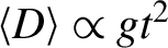 $\left\langle D\right\rangle \propto {gt}^2$, which is well-known bubble size evolution in the turbulent mixing as is discussed in Section 2.10.
Proton backlight image of the magnetic field generated by Rayleigh–Taylor instability of a foil accelerated by laser ablation[Reference Gao, Nilson, Igumenschev, Fiksel, Yan, Davies, Martinez, Smalyuk, Haines, Blackman, Froula, Betti and Meyerhofer35].

An experimental study of magnetic turbulence was performed with the configuration and time evolution of plasmas as shown in Figure 10[Reference Meinecke, Tzeferacos, Bell, Bingham, Clarke, Churazov, Crowston, Doyle, Drake, Heathcote, Koenig, Kuramitsu, Kuranz, Lee, MacDonald, Murphy, Notley, Park, Pelka, Ravasio, Reville, Sakawa, Wan, Woolsey, Yurchak, Miniati, Schekochihin, Lamb and Gregori33]. Plasma jets are designed to collide at the center to allow almost stationary magnetic turbulence evolving at the center, where a probe measures the magnetic field. Note that the laser and target condition are the same in both, right and left, but the Schlieren image looks different because of technology. The jet head-on collision generates a small-scale magnetic field by the Biermann battery and the magnetic field is expected to alter the scale via nonlinear coupling to settle down to a stationary state over time. The power spectrum of the magnetic field energy, 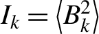 ${I}_k=\left\langle {B}_k^2\right\rangle$, is plotted to show that
  ${I}_k\propto {k}^{-1.9}$. It is also pointed out the the case of one jet results in
  ${I}_k\propto {k}^{-11/3}$.
Magnetic turbulence experiment driven by the Biermann battery effect in two colliding jets. Black is by Schlieren image[Reference Meinecke, Tzeferacos, Bell, Bingham, Clarke, Churazov, Crowston, Doyle, Drake, Heathcote, Koenig, Kuramitsu, Kuranz, Lee, MacDonald, Murphy, Notley, Park, Pelka, Ravasio, Reville, Sakawa, Wan, Woolsey, Yurchak, Miniati, Schekochihin, Lamb and Gregori33].

The dynamo effect has also been studied with a complicated target using the OMEGA laser[Reference Tzeferacos, Rigby, Bott, Bell, Bingham, Casner, Cattaneo, Churazov, Emig, Fiuza, Forest, Foster, Graziani, Katz, Koenig, Li, Meinecke, Petrasso, Park, Remington, Ross, Ryu, Ryutov, White, Reville, Miniati, Schekochihin, Lamb, Froula and Gregori34]. The advanced precision computation has been done with the magnetohydrodynamics (MHD) code FLASH[Reference Tzeferacos, Rigby, Bott, Bell, Bingham, Casner, Cattaneo, Churazov, Emig, Flocke, Fiuza, Forest, Foster, Graziani, Katz, Koenig, Li, Meinecke, Petrasso, Park, Remington, Ross, Ryu, Ryutov, Weide, White, Reville, Miniati, Schekochihin, Froula, Gregori and Lamb36]. It is demonstrated using laser-produced colliding plasma flows that turbulence is indeed capable of rapidly amplifying seed fields to near equipartition with the turbulent fluid motions. To generate magnetic field and turbulent hydrodynamic motion, each plasma jet from both sides is modified to be turbulent by passing through a grid before the collision of both plasma flows. The X-ray emission in the colliding region is found to have a power spectrum of Kolmogorov type  ${k}^{-5/3}$, whereas the power of magnetic turbulence is steeper than
  $1\sim 5/3$. It is concluded that the energy equipartition was established as
  ${B}_{\mathrm{max}}\le 430$ kG, which leads to
 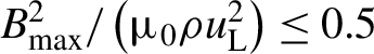 ${B}_{\mathrm{max}}^2/\left({\mu}_0\rho {u}_{\mathrm{L}}^2\right)\le 0.5$, where
  $\rho {u}_{\mathrm{L}}^2$ is kinetic energy of the fluid turbulence.
Plasma flows with different velocities in a collisionless system induce Weibel instability and the magnetic field grows exponentially from the thermal noise. As explained in the following section, the magnetic field becomes turbulent through magnetic reconnection and a nonlinear mechanism. Using ultra-intense laser with 30 fs pulse, Weibel instability is induced on the target plasma to be measured with another laser beam[Reference Tzeferacos, Rigby, Bott, Bell, Bingham, Casner, Cattaneo, Churazov, Emig, Flocke, Fiuza, Forest, Foster, Graziani, Katz, Koenig, Li, Meinecke, Petrasso, Park, Remington, Ross, Ryu, Ryutov, Weide, White, Reville, Miniati, Schekochihin, Froula, Gregori and Lamb36]. In this experiment, magnetic field is seeded by the Weibel instability of electron motion and the magnetic field become in turbulent state after the pulse. In Figure 11, the time evolution of observed power spectra of magnetic energy 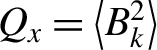 ${Q}_x=\left\langle {B}_k^2\right\rangle$ is plotted a sufficient time after the laser pulse. It is clear that
 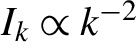 ${I}_k\propto {k}^{-2}$ is seen for a long time. This power law is almost the same as in Ref. [Reference Meinecke, Tzeferacos, Bell, Bingham, Clarke, Churazov, Crowston, Doyle, Drake, Heathcote, Koenig, Kuramitsu, Kuranz, Lee, MacDonald, Murphy, Notley, Park, Pelka, Ravasio, Reville, Sakawa, Wan, Woolsey, Yurchak, Miniati, Schekochihin, Lamb and Gregori33]. Regardless of Biermann battery or Weibel instability, there should be a physics leading to the power spectrum with
  ${k}^{-2}$. Note that both mechanisms interplay in short-pulse laser plasma[Reference Mondal, Narayanan, Ding, Lad, Hao, Ahmad, Wang, Sheng, Sengupta, Kaw, Das and Kumar37].
It should be noted that the Biermann battery is the source of magnetic field in MHD, where the fluid is assumed to be a single fluid, whereas Weibel instability is possible in systems with at least two fluids for cold plasmas. However, the two different experiments concluded with the same turbulent spectrum with  ${k}^{-2}$ power law. There should be the same physics supporting the magnetic turbulence with such spectrum. It is well known that the Navier–Stokes equation allows the Kolmogorov spectrum with power law
  ${k}^{-5/3}$. It should be noted that the energy flow is cascade in three dimensions, whereas it is inverse cascade for two dimensions. In the case of a magnetic field, magnetic reconnection is important as a nonlinear process to induce always inverse-cascade energy flow in two and three dimensions. It is challenging to identify the power law and physics behind for magnetic turbulence, because it may also affect the transport and particle acceleration in the universe.
Power spectrum of the magnetic field spatial profiles measured at different pump-probe delays. The inset shows the power spectra derived from two-dimensional PIC simulations[Reference Mondal, Narayanan, Ding, Lad, Hao, Ahmad, Wang, Sheng, Sengupta, Kaw, Das and Kumar37].

It is also important to study an MHD-type magnetic instability generated by the return current in front of a collisionless shock emitting highly relativistic cosmic rays. This is called Bell instability and is expected to maintain the magnetic turbulence necessary for DSA in the universe[Reference Bell38].
It is noted that an extensive review of magnetic turbulence is given in Ref. [Reference Gregori, Reville and Miniati39].
2.3 Collisionless shock experiments
Most shock waves in astrophysics are not hydrodynamic shock, but collisionless shock waves. The shock waves are obtained mathematically as a jump solution of the stationary hydrodynamic equation. Physical structure of the shock jump region is determined by a dissipation mechanism. The hydrodynamic shock structure is given by collisional viscosity, whereas the collisionless shock is due to plasma flow reflection by a self-generated magnetic field. Magnetic turbulence due to magnetic instability works as effective dissipation to charged particles to form such a collisionless shock structure. The collisionless shocks in the universe are roughly divided into nonrelativistic and relativistic. High-Mach-number collisionless experiments are very important relating to acceleration of cosmic rays around the shock front. This acceleration mechanism is called DSA and mainly applicable to the nonrelativistic shock case[Reference Schure, Bell, Drury and Bykov40].
A typical example of nonrelativistic collisionless shock is blast waves by supernova remnants (SNRs)[Reference Cassam-Chenaï, Hughes, Reynoso, Badenes and Moffett41]. Their expansion velocities are around  ${10}^3{-}{10}^4$ km/s (about 1% of the light speed). Only intense lasers can produce such high-velocity flow in ablation plasma in laboratory. It was proposed to use counter-streaming ablation plasmas to generate high-Mach-number collisionless shock waves to model collisionless shocks observed as expanding shocks of SNRs[Reference Takabe, Kato, Sakawa, Kuramitsu, Morita, Kadono, Shigemori, Otani, Nagatomo, Norimatsu, Dono, Endo, Miyanishi, Kimura, Shiroshita, Ozaki, Kodama, Fujioka, Nishimura, Salzman, Loupias, Gregory, Koenig, Waugh, Woolsey, Kato, Li, Dong, Wang, Zhang, Zhao, Wang, Wei, Shi, Zhao, Zhang, Wen, Zhang, Hu, Liu, Ding, Zhang, Tang, Zhang, Zheng, Sheng and Zhang42, Reference Kato and Takabe43]. A shock wave of an SNR propagates spherically and its local view is as shown in Figure 12(a), where the shock front propagates from the left to right. Behind the shock front, the plasma is compressed and has flow velocity lower than the shock front. The flow velocities are seen as in Figure 12(b) in the frame moving with the shock front. In the proposal of the counter-streaming plasma experiment, the laser ablation plasmas are designed to produce two shock waves propagating to both sides as shown in Figure 12(c), where the red arrows are ablation flow and green arrows are shock velocities. In Figure 12(d), a shock experiment is schematically shown, where purple indicates multilaser beams. Targets placed on both sides produce plasma flows shown in white to generate dense shocked plasma in the counter-streaming region. The increase of temperature and density is measured at the central red point with Thomson scattering diagnostics.
Schematics for modeling astrophysical shock and counter streaming plasmas. The black layer is the shock front. The green arrow shows the velocity of shock front and the red is the flow in the compressed region by the shock wave. In the frame moving with the shock front, the flow velocities of the front and behind are shown as red arrows. The counter-streaming plasmas can model such shock wave formation in both sides of the plasmas. Laser ablation plasma is used to model the counter streaming plasma situation.

In Ref. [Reference Takabe, Kato, Sakawa, Kuramitsu, Morita, Kadono, Shigemori, Otani, Nagatomo, Norimatsu, Dono, Endo, Miyanishi, Kimura, Shiroshita, Ozaki, Kodama, Fujioka, Nishimura, Salzman, Loupias, Gregory, Koenig, Waugh, Woolsey, Kato, Li, Dong, Wang, Zhang, Zhao, Wang, Wei, Shi, Zhao, Zhang, Wen, Zhang, Hu, Liu, Ding, Zhang, Tang, Zhang, Zheng, Sheng and Zhang42], it was concluded that only National Ignition Facility (NIF) at LLNL can generate the collisionless shock mediated by Weibel instability, because it takes a relatively long time for the magnetic field to grow from the thermal noise to the turbulent stage and in addition the structure of shock wave is so gentle that relatively large-scale counter-streaming plasmas should be produced to identify the shock wave formation. A typical snapshot of a PIC simulation is shown in Figure 13 at a time after the collisionless shock wave is produced. In Figure 13[Reference Kato and Takabe43], the number density of ions, current density, and magnetic field strength are plotted in the x–y plane, where the simulation starts with uniform flow to the right and the right boundary is assumed to be a perfect reflection wall. The simulation is to model the plasma dynamics of the left half of Figure 12(c). Note that such collisionless shock sustained by magnetic turbulence induced by Weibel instability has its structure of filaments in the shock front region. The thickness of shock wave is about 200–300 in the x-direction as shown in Figure 13.
A snapshot of density, current density and magnetic field strength from a two-dimensional PIC simulation at the time when the shock wave region with filamentary structure is formed around the center of the figures. The density profile averaged in the y-direction clearly shows the density change with the thickness of about 100–200 in the x-direction[Reference Takabe, Kato, Sakawa, Kuramitsu, Morita, Kadono, Shigemori, Otani, Nagatomo, Norimatsu, Dono, Endo, Miyanishi, Kimura, Shiroshita, Ozaki, Kodama, Fujioka, Nishimura, Salzman, Loupias, Gregory, Koenig, Waugh, Woolsey, Kato, Li, Dong, Wang, Zhang, Zhao, Wang, Wei, Shi, Zhao, Zhang, Wen, Zhang, Hu, Liu, Ding, Zhang, Tang, Zhang, Zheng, Sheng and Zhang42, Reference Kato and Takabe43].

The Weibel instability starts to grow and evolve from the left to right in the snapshot in Figure 13. As the linear growth rate is larger for shorter wavelength in the y-direction, the thin filaments grow first and the filament coalescence in the later nonlinear phase can be seen toward the right direction. This nonlinear evolution can be explained theoretically and is reported in Ref. [Reference Takabe44]. Its essential physics is due to the nonlinear effect by magnetic pressure force and magnetic reconnection. In Figure 14, a schematic of the current filament coalescence is shown before reconnection (left) and after reconnection (right). This is a cut view of the three-dimensional Weibel instability in the plane yz perpendicular to the plasma flows in the x-direction. The force working among the circular filaments are shown with red (attractive force) and black (repulsive flow) due to Lorentz  $\overrightarrow{v}\times \overrightarrow{B}$ force. As the attractive force works among the filaments with the same directional current, the Lorentz force works to reconnect the filaments to make thicker filaments.
Schematics of the cut view of the nonlinear stage of Weibel instability. The collisionless plasma flows perpendicularly to the figure surface. In the nonlinear phase of Weibel instability, current filaments are produced as in (a). Then, Lorentz force between the current and induced magnetic field works as shown in (a). If the purple circle is the current channel from the top to bottom direction of the figure, the force shown with red is attractive force, whereas the force with a channel with the opposite directional current in green is repulsive. As a result, the filaments become larger by reconnection in a later time as shown in (b).

This filament coalescence has been demonstrated experimentally as shown in Figure 15[Reference Park, Huntington, Fiuza, Drake, Froula, Gregori, Koenig, Kugland, Kuranz, Lamb, Levy, Li, Meinecke, Morita, Petrasso, Pollock, Remington, Rinderknecht, Rosenberg, Ross, Ryutov, Sakawa, Spitkovsky, Takabe, Turnbull, Tzeferacos, Weber and Zylstra45]. It is clear that the mean value of the filament size  $<\lambda >$ increases linearly in time. This is the so-called inverse cascade in the wavenumber
  $k$ space in the power spectrum. It is very different from the conventional fluid turbulence showing cascade to reach the Kolmogorov spectrum. A simple model equation is found to explain such computational and experimental results[Reference Takabe44]. By modeling the growth of each mode with the amplitude given by the reconnection process, the linear growth of the filament size can be reproduced. It is also found that when the thickness of typical filaments becomes almost equal to the Larmor radius of an ion, the shock wave is formed.
Time evolution of measured and computational size of filaments in the nonlinear phase of Weibel instability in the counter-streaming plasma. It is found that the average size of filaments increases in proportion to time with an effective speed of the value shown.

The formation of collisionless shock wave and production of nonthermal electrons by the DSA process have been demonstrated experimentally with the use of the NIF[Reference Fiuza, Swadling, Grassi, Rinderknecht, Higginson, Ryutov, Bruulsema, Drake, Funk, Glenzer, Gregori, Li, Pollock, Remington, Ross, Rozmus, Sakawa, Spitkovsky, Wilks and Park46]. Figure 16(a) shows electron energy spectra measured in the experiment. The data in blue is the result in the case where the laser is irradiated only on one side. On the other hand, two red lines are taken in the experiments where the laser is irradiated on both targets to generate the counter-streaming plasma flow. Figure 16(b) is the electron energy spectrum obtained in the corresponding PIC simulation. A power-law evolution of spectra typical to nonthermal particle acceleration such as cosmic rays is obtained to explain the NIF experimental result. The maximum energy is about 1 MeV, whereas it is known that SNR collisionless shocks accelerate up to 10 ${}^{15}$ eV. This difference of nine orders is due to the difference of time scales of acceleration and the strength of magnetic field. It should be noted that it is not so difficult to extrapolate the model experiment to the cosmic rays. It should be noted that such acceleration is applicable to nonrelativistic shock case, whereas it is not clear whether the same physics works for relativistic collisionless shocks. We need some new acceleration physics mechanisms for cosmic rays with energy more than 10
 ${}^{15}$ eV. The laser model experiment for highly relativistic particle acceleration in such regime is discussed in Section 2.4, but it is not acceleration by collisionless shock waves.
Demonstration of the nonthermal high-energy electrons produced experimentally in the counter-streaming ablation plasma flow as shown with two red lines in (a), whereas far fewer high-energy electrons are measured in the case of single flow. This is indirect proof of the formation of collisionless shock and particle acceleration, which is obtained in two-dimensional PIC simulation as shown in (b)[Reference Fiuza, Swadling, Grassi, Rinderknecht, Higginson, Ryutov, Bruulsema, Drake, Funk, Glenzer, Gregori, Li, Pollock, Remington, Ross, Rozmus, Sakawa, Spitkovsky, Wilks and Park46].

The formation of nonrelativistic collisionless shocks in the laboratory with ultra-high-intensity lasers has been demonstrated by an international team ACSEL after about one decade from the initial proposal. The microphysics behind shock formation and dissipation and the detailed shock structure have been analyzed, illustrating that the Weibel instability plays a crucial role in the generation of strong subequipartition magnetic fields that isotropize the incoming flow and lead to the formation of a collisionless shock, similar to what occurs in astrophysical scenarios. The possibility of generating such collisionless shocks in the laboratory opens the way to the direct study of the physics associated with astrophysical shocks.
After the success of Weibel-mediated shock research, a magnetized collisionless shock experiment is now ongoing[Reference Schaeffer, Fox, Haberberger, Fiksel, Bhattacharjee, Barnak, Hu, Germaschewski and Follett47]. It is expected that the shock formation time is shorter than the Weibel case so that even with the OMEGA laser we can expect shock formation.
A design to generate relativistic collisionless shock with ultra-intense lasers is also proposed and it was computationally studied in Ref. [Reference Fiuza, Fonseca, Tonge, Mori and Silva48]. The relativistic collisionless shocks are speculated to be source of ultra-high-energy cosmic rays (UHECRs) with energy more than  ${10}^{15}$ eV.
In astrophysics, relativistic collisionless shocks are usually generated in electron–positron plasmas. Positron production by ultra-intense lasers has been studied intensively, for example, in Ref. [Reference Chen, Fiuza, Link, Hazi, Hill, Hoarty, James, Kerr, Meyerhofer, Myatt, Park, Sentoku and Williams49]. Such pair plasma collisionless shock formation requires the group of pair plasma larger than the Debye length. With use of structured pillar-type targets and enhancement of positron production from  ${10}^{10}$ to
  ${10}^{12}$ per shot[Reference Jiang, Link, Canning, Fooks, Kempler, Kerr, Kim, Krieger, Lewis, Wallace, Williams, Yalamanchili and Chen50], it is now almost possible to carry out relativistic collisionless shock with use of counter-propagating electron–positron beams produced from the rear of the two targets as in the PIC result shown in Figure 17[Reference Chen, Fiuza, Link, Hazi, Hill, Hoarty, James, Kerr, Meyerhofer, Myatt, Park, Sentoku and Williams49].
PIC simulations of the counter-streaming of relativistic pair plasmas for laser-driven laboratory parameters. Magnetic field structure and transversely averaged density profile (inset). The formation of a shock with near-future laser systems: (a) 7 kJ; (b) 22 kJ[Reference Chen, Fiuza, Link, Hazi, Hill, Hoarty, James, Kerr, Meyerhofer, Myatt, Park, Sentoku and Williams49].

In Ref. [Reference Lemoine, Gremillet, Pelletier and Vanthieghem51], a comprehensive theoretical model of relativistic collisionless pair shocks mediated by the current filamentation instability was presented. The noninertial frame is used in which this instability is of a mostly magnetic nature, and describes at a microscopic level the deceleration and heating of the incoming background plasma through its collisionless interaction with the electromagnetic turbulence. This model compares well to large-scale 2D3V (two-dimensional in space and three-dimensional in velocity space) PIC simulations, and provides an important touchstone for the phenomenology of such plasma systems.
2.4 Stochastic particle acceleration and cosmic rays
Let us introduce the observation data of cosmic rays accumulated in more than 10 observatories. It is updated regularly and the last update in 2020 is shown in Figure 18[Reference Evoli, Blasi, Amato and Aloisio52]. All data are from each observatory identified by color and name. Most of the cosmic-ray particles coming from the space are protons. The highest proton energy is about 1 J ( $\sim$10
 ${}^{19}$ eV). It is thought that cosmic-ray particles of around 1 GeV stem from the Sun, up to 10
 ${}^{15}$ eV (1 PeV: so-called ‘knee’) is mainly due to SNRs in our galaxy, and higher-energy cosimic rays are from the outside of our galaxy. The physical reason why the petaelectronvolt is critical for the source to be galactic or not is that a proton with energy of more than 1 PeV cannot be confined inside of our galaxy by the diffusive property stemming from the background magnetic turbulence. The figure also indicates how many particles are observed per unit square and unit time.
The observation data of energy spectra of cosmic rays updated on December 2020. All results obtained in 19 observatories worldwide are plotted with different colors. Most of the cosmic rays are protons and it is clear that all data has the same power law below the knee and the ankle. The power law shows some nonthermal acceleration physics in the universe. The collision energy of the largest accelerator LHC is also indicated as a reference[Reference Evoli, Blasi, Amato and Aloisio52].

The standard theory for explaining the generation of cosmic rays in the universe is the well-known DSA[Reference Blandford and Eichler53]. In this model, a charge particle is confined by a magnetic field before and after the collisionless shock wave surface and reciprocates many times, and the energy gradually increases. This is the acceleration mechanism seen in the PIC simulation and speculated to be demonstrated experimentally with NIF as shown in Figure 16. Therefore, energy increase via one bounce  $\Delta E$ is assumed much smaller than its energy
  $E$,
$E$,  $\Delta E/E\ll 1$. This is the reason why it is called ‘diffusive’. This model is very successful in explaining the power-law spectrum over approximately 20 orders of magnitude observed worldwide.
However, DSA has difficulty in applying it to the case of relativistic shock waves. An accelerating particle has to pass many times through a shock front that propagates at almost the speed of light. Chen et al. proposed wakefield acceleration in the relativistic regime, where a stochastic wakefield generated by an Alfvén wave, for example, in AGN jets in Figure 19, can accelerate particles via the ponderomotive force of the wake[Reference Chen, Tajima and Takahashi54]. Note that Lorentz factor of AGN jets is thought to be about 10–20. In Ref. [Reference Chen, Tajima and Takahashi54], the wake acceleration is modeled also by a diffusion-type Fokker–Planck (FP) equation:
 \begin{align}\frac{\partial f\left(p,t\right)}{\partial t}=\frac{\partial^2}{\partial {\left[p\right]}^2}{\int}_{-\infty}^{+\infty}\mathrm{d}\left(\Delta p\right)\frac{\Delta {p}^2}{2}\Psi \left(p,\Delta p\right)f\left(p,t\right)\end{align}
Image of AGN jets from the central massive blackhole [from Wikipedia].

By assuming the transition probability density  $\Psi$ is constant and a stationary solution, the power law
  $f(p)\propto {p}^{-2}$ is concluded.
A model experiment of stochastic wake field acceleration has been carried out with relativistic lasers with field strength  ${a}_0>1$ (see Section 2.3). The details of the experiment, analysis and results are given in Section 3 in this review paper and a power-law spectrum with
  ${p}^{-2}$ is obtained for electrons in the range of
  $10{-}100$ MeV. It is challenging to study the origin of cosmic rays with relativistic lasers and the ponderomotive force of the induced wake field. Intuitively, it seems that the energy conversion efficiency is small. Recently, the first author proposed a new physics to explain the cosmic-ray acceleration directly by the electromagnetic wave field in a random system[Reference Takabe55].
Regardless of whether it is an Alfvén wave or laser wave, an electron oscillation becomes nonlinear even in a plane wave, because the  $\overrightarrow{v}\times \overrightarrow{B}$ term becomes important. Then, the electron motion becomes chaotic when an external force or abrupt change of wave phase is loaded into the oscillation system as perturbation[Reference Takabe55]. If
  $\Delta p$ by the perturbation is small,
  $\Delta p/p\ll 1$, the electron distribution function is approximately governed by the FP-type equation. However, the increase of laser intensity and relativistic nonlinearity becomes strong, and then it is necessary to consider a model for the case
  $\Delta p/p\approx O(1)$. As the FP equation is based on Taylor expansion, it is called local diffusion in momentum space. On the other hand, we have to consider the case for nonlocal jump diffusion.
This nonlocal jump is known as Levy’s jump[Reference Takabe55]. This concept is widely used for anomalous transport and nonlocal transport due to turbulence in real space. The change of distribution function by such nonlocal transport in momentum space is modeled with the fractional FP equation (FFPE) in the form
 \begin{align}\frac{\partial f\left(p,t\right)}{\partial t}={D}_{\alpha}\frac{\partial^{\alpha }}{\partial {\left|p\right|}^{\alpha }}f\left(p,t\right),\end{align}
where  $\alpha$ is the fractal index and
  $0<\alpha <2$. The definition of the operator is given in Ref. [Reference Takabe55]. The FP equation is the case
  $\alpha =2$ and
  $\Psi \left(\Delta p\right)$ is a Gaussian case. As the Gaussian decays exponentially for large
  $\Delta p,$ it is used for the probability of local diffusion. It is known that with decrease of
  $\alpha$, the probability
  $\Psi \left(\Delta p\right)$ spreads wider with a power-law tail. For the case of
  $\alpha =1$,
  $\Psi \left(\Delta p\right)\propto {\left(\Delta p\right)}^{-2}$ and Lorentzian solution of Equation (5) is obtained[55]:
 \begin{align}f\left(p,t\right)=\frac{1}{\pi Dt}\frac{1}{1+\left(\frac{p}{Dt}\right)}\propto {p}^{-2}.\end{align}
The distribution function after an acceleration time is shown in Figure 20 to compare with that in Section 2.3. We have assumed that the electrons are accelerated not by the wake but by the laser field itself. As the diffusion in energy space is not only nonlocal but also local, the distributions in Figure 20 are shown for 100 % nonlocal to 1% nonlocal[Reference Takabe55]. It is surprising to find that a few percent of probability of nonlocal process agrees with the experimental energy spectrum in Section 2.3.
Electron distribution functions obtained from the linear combination of nonlocal and local diffusion models[Reference Takabe55]. In the heating model, the blue line case is obtained with 100% nonlocal heating, whereas the orange line is for 10% nonlocal and green is for 1% nonlocal heating.

Power-law spectra of electron energy have also been observed in the LFEX experiment in Osaka[Reference Kojima, Hata, Iwata, Arikawa, Morace, Sakata, Lee, Matsuo, Law, Morita, Ochiai, Yogo, Nagatomo, Ozaki, Johzaki, Sunahara, Sakagami, Zhang, Tosaki, Abe, Kawanaka, Tokita, Nakai, Nishimura, Shiraga, Azechi, Sentoku and Fujioka56]. In Figure 21, the experimental data of the electron energy distribution is shown with red circles in log–log space. Comparing the flat and power-law spectrum shown in blue in Figure 20, it can be said that the red points in Figure 21 may be explained by taking account of such nonlocal stochastic process owing to the distorted relativistic laser field in ablating plasmas, where the strength parameter is  ${a}_0=2.4$ and the relativistic nonlinearity has already been shown to be important[Reference Takabe55]. It is a very interesting proposal to study the maximum electron energy and the power-law number of the nonthermal electrons as a function of laser strength parameter
  ${a}_0$, laser pulse duration, and so on. It would be beneficial to study a new physical mechanism of the acceleration of cosmic rays in the universe, especially for UHECRs with particle energy more than
  ${10}^{15}$ eV (1 PeV). It is clear that the spectrum can be reproduced with 50% local (Gaussian) and 50% nonlocal (Lorentzian) acceleration. In this experiment, the strength parameter is
  ${a}_0=2.4$ and relativistic nonlinearity already became important.
Electron distribution function obtained in the LFEX experiment at Osaka (courtesy of S. Kojima)[Reference Kojima, Hata, Iwata, Arikawa, Morace, Sakata, Lee, Matsuo, Law, Morita, Ochiai, Yogo, Nagatomo, Ozaki, Johzaki, Sunahara, Sakagami, Zhang, Tosaki, Abe, Kawanaka, Tokita, Nakai, Nishimura, Shiraga, Azechi, Sentoku and Fujioka56].

This new mechanism could be seen in astrophysics. A relativistic electromagnetic field is generated around pulsars. It is shown in PIC code that electromagnetic waves are generated in front of a relativistic collisionless shock. Although both are noncoherent waves like a laser, it is reported that their strength is relativistic such as  ${a}_0>3$[Reference Iwamoto, Amano, Hoshino, Matsumoto, Niemiec, Ligorini, Kobzar and Pohl57]. In addition, the electromagnetic waves have random phase because of filamentation instability, suggesting that electrons are accelerated randomly with large phase jump nonlocally in energy space[Reference Takabe55].
2.5 Electron–positron plasma by ultra-intense lasers
Electron-positron pair plasmas are found in various extreme astrophysical objects, such as pulsars, bipolar outflows, AGN, and gamma-ray bursts (GRBs). Producing a pair plasma with similar conditions in the laboratory is extremely challenging but could significantly deepen the understanding of these exotic objects. With the advances in high-intensity laser technology, several methods for pair production have been either demonstrated or proposed, with different mechanisms dominating the physics in different regimes of laser intensity.
It was first reported in Ref. [Reference Cowan, Perry, Key, Ditmire, Hatchett, Henry, Moody, Moran, Pennington, Phillips, Sangster, Sefcik, Singh, Snavely, Stoyer, Wilks, Young, Takahashi, Dong, Fountain, Parnell, Johnson, Hunt and Kühl58] that the petawatt laser at LLNL achieved laser intensity of over  ${10}^{20}$ W/cm
 ${}^2$ and generated electron–positron pairs from gold foils. It has opened a new regime of laser–matter interactions in which the quiver motion of plasma electrons is fully relativistic with energies extending well above the threshold for nuclear processes. Few megaelectronvolt electrons are produced in ultra-intense laser–solid interactions. The generation of hard bremsstrahlung, photonuclear reactions and preliminary evidence for electron–positron pair production are shown.
A theoretical study has been reported to explain the physical process for the positron production in the experiment with the use of the relativistic FP equation to the electrons produced by the petawatt laser as well as the positrons generated[Reference Nakashima and Takabe59]. There are a few processes that create electron–positron pairs. Two processes, the trident process and the Bethe–Heitler (BH) process, are dominant. It is found that the total positron yield increases logarithmically with the increase of the laser intensity, and the resultant energy distribution of the created positron is found to have a peak near the energy of  $1{-}2$ MeV. Later it was demonstrated that the group of electron–positron pairs is generated as a form of beam due to the acceleration by the ambipolar field, which is generated by the hot electrons escaping from the rear of the solid target.
Although it has been theoretically studied since the 1970s, the use of lasers as a valuable new positron source was not demonstrated experimentally until the petawatt-class short pulse lasers were developed. In 2008 and 2009, in a series of experiments performed at the LLNL, a large number of positrons were observed after shooting a millimeter-thick solid gold target[Reference Chen, Wilks, Bonlie, Chen, Cone, Elberson, Gregori, Meyerhofer, Myatt, Price, Schneider, Shepherd, Stafford, Tommasini, Van Maren and Beiersdorfer60]. Up to  $2\times {10}^{10}$ positrons/shot ejected at the back of approximately millimeter-thick gold targets were detected.
The experimental results obtained on three different laser facilities were reported in Ref. [Reference Chen, Fiuza, Link, Hazi, Hill, Hoarty, James, Kerr, Meyerhofer, Myatt, Park, Sentoku and Williams49]. Directed laser-driven relativistic electron–positron jets with up to 30 times larger yields than obtained previously and a quadratic  $\left(\sim {E}_L^2\right)$ dependence of the positron yield on the laser energy were reported. This is shown in Figure 22, where all experimental data are enhanced compared with poderomotive scaling, owing to the higher hot electron temperature predicted by Pukov. This favorable scaling stems from a combination of higher-energy electrons due to increased laser intensity and the recirculation of megaelectronvolt electrons in the millimeter-thick target. Based on this scaling, first principles simulations predict the possibility of using such electron–positron jets, produced at upcoming high-energy laser facilities, to probe the physics of relativistic collisionless shocks in the laboratory.
Experimental data (blue with error bars) of positron numbers. Others are computational results or models[Reference Chen, Fiuza, Link, Hazi, Hill, Hoarty, James, Kerr, Meyerhofer, Myatt, Park, Sentoku and Williams49].

The electron temperature largely determines the positron yield from the BH mechanism, so a key to higher positron production is the production of hotter electrons. In addition to increasing the laser intensity, substantial enhancement in electron energies can be obtained by manipulating the laser–plasma interaction using a structured front surface target[Reference Takabe61]. Substantial increase of hot electron temperature is demonstrated with a Si array target as shown in Figure 23. An enhanced number of positrons have been demonstrated experimentally[Reference Jiang, Ji, Audesirk, George, Snyder, Krygier, Poole, Willis, Daskalova, Chowdhury, Lewis, Schumacher, Pukhov, Freeman and Akli62]. Experiments using this type of setup have produced up to  ${10}^{12}$ pairs/shot, which is the highest yield reported to date by the use of lasers[Reference Jiang, Link, Canning, Fooks, Kempler, Kerr, Kim, Krieger, Lewis, Wallace, Williams, Yalamanchili and Chen50].
Structured targets result in a dramatic increase in the number and temperature of hot electrons[Reference Jiang, Ji, Audesirk, George, Snyder, Krygier, Poole, Willis, Daskalova, Chowdhury, Lewis, Schumacher, Pukhov, Freeman and Akli62].

2.6 EOS experiments
EOS of highly compressed matter is an important ingredient to study high-pressure physics, laser fusion, planetary interior[Reference Guillot, Gautier and Schubert63, Reference Queloz64], etc. High-intensity laser is now a strong tool to study such EOS of a variety of materials by coupling with new diagnostic methods developed in the last 20 years. Let us briefly describe the important progress of the EOS experiment with intense lasers. The insulator–metal phase transition at high density is a long-standing question pointed out by Wigner–Huntington in 1935[Reference Wigner and Huntington65]. The high-pressure community has tried to realize a metallic state by compressing solid/liquid hydrogen using a diamond anvil cell (DAC). It is reported that the Wigner–Huntington insulator–metal transition was experimentally observed with DAC[Reference Dias and Silvera66, Reference Silvera and Dias67]. Laser shock experiment has also challenged this ground-breaking physics by decreasing the temperature of the compressed state with tailoring of laser pulse shape.
In the last few decades, a new diagnostics VISAR and a streaked optical pyrometer (SOP) to measure the shock and piston velocities have been developed with use of the Doppler shift of the irradiated laser for diagnostic purposes[Reference Celliers, Collins, Da Silva, Gold and Cauble68, Reference Celliers, Collins, Bradley, Moon, Munro, Cauble, Gold, Da Silva, Weber, Wallace, Hammel and Hsing69]. By use of this diagnostic technique, the shock and piston velocities are measured precisely. Then, it is possible to obtain the shock jump relation experimentally with the jump relation:
 \begin{align}{\rho}_1&={\rho}_0\frac{U_{\mathrm{s}}}{U_{\mathrm{s}}-{U}_{\mathrm{p}}},\notag\\{}{P}_1&={P}_0+{\rho}_0{U}_{\mathrm{s}}{U}_{\mathrm{p}},\notag\\{}{\epsilon}_1&={\epsilon}_0+\frac{1}{2}\left({P}_1-{P}_0\right)\left(\frac{1}{\rho_0}-\frac{1}{\rho_1}\right).\end{align}
 With measured values of  ${U}_{\mathrm{s}}$ and
  ${U}_{\mathrm{p}}$ for a single shock, the thermodynamic state described by suffix ‘1’ after the shock passage is given by Equation (7) for the values at initial state ‘0’. This curve of density versus pressure is called the Hugoniot curve.
In addition, several new facilities of X-ray free-electron laser (XFEL) have opened as user facility and the coherent, bright X-ray source is now available for clear imaging of such laser-driven shock experiments. Combination of lasers and XFEL is the new trend to make it possible to measure the properties of laser-compressed matter under extreme conditions[Reference Schropp, Hoppe, Meier, Patommel, Seiboth, Ping, Hicks, Beckwith, Collins, Higginbotham, Wark, Lee, Nagler, Galtier, Arnold, Zastrau, Hastings and Schroer70].
Modern shock experiments are done not only with lasers but also gas guns and Z-pinch facilities[Reference Sinars, Sweeney, Alexander, Ampleford, Ao, Apruzese, Aragon, Armstrong, Austin, Awe, Baczewski, Bailey, Baker, Ball, Barclay, Beatty, Beckwith, Bell, Benage, Bennett, Blaha, Bliss, Boerner, Bourdon, Branch, Brown, Campbell, Campbell, Chacon, Chandler, Chandler, Christenson, Christison, Christner, Clay, Cochrane, Colombo, Cook, Coverdale, Cuneo, Custer, Dasgupta, Davis, Desjarlais, Dolan, Douglass, Dunham, Duwal, Edens, Edwards, Evstatiev, Farfan, Fein, Field, Fisher, Flanagan, Flicker, Furnish, Galloway, Gard, Gardiner, Geissel, Giuliani, Glinsky, Gomez, Gomez, Grim, Hahn, Haill, Hamlin, Hammer, Hansen, Hanshaw, Harding, Harvey-Thompson, Headley, Herrmann, Hess, Highstrete, Hurricane, Hutsel, Jennings, Johns, Johnson, Johnston, Jones, Jones, Jones, Kalita, Kamm, Kellogg, Kiefer, Kimmel, Knapp, Knudson, Kreft, Laity, Lake, Lamppa, Langston, Lash, LeChien, Leckbee, Leeper, Leifeste, Lemke, Lewis, Lewis, Loisel, Looker, Lopez, Lucero, MacLaren, Magyar, Mangan, Martin, Mattsson, Matzen, Maurer, Mazarakis, McBride, McLean, McCoy, McKee, McKenney, Miles, Mills, Mitchell, Moore, Myers, Nagayama, Natoni, Owen, Patel, Peterson, Pointon, Porter, Porwitzky, Radovich, Raman, Rambo, Reinhart, Robertson, Rochau, Root, Rose, Rovang, Ruiz, Ruiz, Sandoval, Savage, Sceiford, Schaeuble, Schmit, Schollmeier, Schwarz, Seagle, Sefkow, Seidel, Shipley, Shores, Shulenburger, Simpson, Slutz, Smith, Speas, Specht, Speir, Spencer, Springer, Steiner, Stoltzfus, Stygar, Thornhill, Torres, Townsend, Tyler, Vesey, Wakeland, Webb, Weinbrecht, Weis, Welch, Wise, Wu, Yager-Elorriaga, Yu and Yu71]. An artistic image of the laser shock experiment is shown in Figure 24. To achieve one-dimensional planar shock, many laser beams are irradiated to obtain the wide surface to drive a shock wave. For diagnostic purposes, a complicated sandwiched target is used. In Figure 24, the target is designed to measure the shock Hugoniot curve. The experimental data have inspired the proposal of several theoretical models. Many modern computations have been published to explain such experimental data, for example, the density functional method, quantum Monte Carlo analysis, and molecular dynamics[Reference McMahon, Morales, Pierleoni and Ceperley72].
Artistic picture of EOS experiment with irradiation of many laser beams (courtesy of LLNL).

The experimental result of the insulator–metal transition of fluid molecular hydrogen was initially reported in experiments with a gas gun[Reference Weir, Mitchell and Nellis73]. The experiment was designed so that a shock wave reverberated held between Al ${}_2$O
 ${}_3$ anvils to compress liquid H
 ${}_2$ or D
 ${}_2$ to pressures of
  $0.93{-}1.8$ Mbar. It was found that the resistivity decreases almost 4 orders of magnitude from 0.9 to 1.4 Mbar and then plateaus to 1.8 Mbar.
This pressure of 1.4 Mbar for insulator–metal transition is very low compared with the static experimental result of 5 Mbar demonstrated with DAC. Shock compression is also used to clarify the critical pressure to change the insulator to metal in fluid deuterium at relatively low temperature. The experimental data are plotted in Figure 25 to find the phase transition boundary curve[Reference Celliers, Millot, Brygoo, McWilliams, Fratanduono, Rygg, Goncharov, Loubeyre, Eggert, Peterson, Meezan, Le Pape, Collins, Jeanloz and Hemley74]. The black solid line inferred by experimental data is the plasma phase transition and the matter becomes conductive because of the increase of thermal free electrons[Reference Celliers, Millot, Brygoo, McWilliams, Fratanduono, Rygg, Goncharov, Loubeyre, Eggert, Peterson, Meezan, Le Pape, Collins, Jeanloz and Hemley74]. The boundary with the black open circles means the points where the band gap becomes about 2 eV, almost a semiconductor.
Phase diagram of hydrogen around the solid state. The marks are experimental data to explore the metallic hydrogen[Reference Celliers, Millot, Brygoo, McWilliams, Fratanduono, Rygg, Goncharov, Loubeyre, Eggert, Peterson, Meezan, Le Pape, Collins, Jeanloz and Hemley74].

It was already mentioned that to obtain the dense matter EOS in a wide range, we have to obtain experimental data by changing the initial condition of density and/or pressure. Using the shock wave transmitting from the quartz reference plate, the Hugoniot curves of the different initial density and pressure have been obtained. The experimental data are plotted in Figure 26[Reference Brygoo, Millot, Loubeyre, Lazicki, Hamel, Qi, Celliers, Coppari, Eggert, Fratanduono, Hicks, Rygg, Smith, Swift, Collins and Jeanloz75] for hydrogen and deuterium for four different initial pressures (density), 1 kbar (0.029 mol/cm ${}^3$), 3 kbar (0.044 mol/cm
 ${}^3$), 7 kbar (0.061 mol/cm
 ${}^3$), and 15 kbar (0.079 mol/cm
 ${}^3$). The corresponding solid lines are theoretical from density functional theory with molecular dynamics methods. It is seen that small change of the initial condition of pressure and density alters the Hugoniot curve substantially.
Shock Hugoniot curves from different initial densities[Reference Brygoo, Millot, Loubeyre, Lazicki, Hamel, Qi, Celliers, Coppari, Eggert, Fratanduono, Hicks, Rygg, Smith, Swift, Collins and Jeanloz75].

2.7 Opacity experiments
The stellar interior is characterized by high density and high temperature and it is well known that the radiation transport is important to transfer the nuclear fusion energy toward the surface. Not only the transport but also the structure of stars strongly depends on the atomic state of the plasma, namely, so-called plasma opacity. Historically, the opacity has been calculated theoretically, especially using computers. Intense laser and Z-pinch facilities have been used for spectroscopic opacity experiments[Reference Sinars, Sweeney, Alexander, Ampleford, Ao, Apruzese, Aragon, Armstrong, Austin, Awe, Baczewski, Bailey, Baker, Ball, Barclay, Beatty, Beckwith, Bell, Benage, Bennett, Blaha, Bliss, Boerner, Bourdon, Branch, Brown, Campbell, Campbell, Chacon, Chandler, Chandler, Christenson, Christison, Christner, Clay, Cochrane, Colombo, Cook, Coverdale, Cuneo, Custer, Dasgupta, Davis, Desjarlais, Dolan, Douglass, Dunham, Duwal, Edens, Edwards, Evstatiev, Farfan, Fein, Field, Fisher, Flanagan, Flicker, Furnish, Galloway, Gard, Gardiner, Geissel, Giuliani, Glinsky, Gomez, Gomez, Grim, Hahn, Haill, Hamlin, Hammer, Hansen, Hanshaw, Harding, Harvey-Thompson, Headley, Herrmann, Hess, Highstrete, Hurricane, Hutsel, Jennings, Johns, Johnson, Johnston, Jones, Jones, Jones, Kalita, Kamm, Kellogg, Kiefer, Kimmel, Knapp, Knudson, Kreft, Laity, Lake, Lamppa, Langston, Lash, LeChien, Leckbee, Leeper, Leifeste, Lemke, Lewis, Lewis, Loisel, Looker, Lopez, Lucero, MacLaren, Magyar, Mangan, Martin, Mattsson, Matzen, Maurer, Mazarakis, McBride, McLean, McCoy, McKee, McKenney, Miles, Mills, Mitchell, Moore, Myers, Nagayama, Natoni, Owen, Patel, Peterson, Pointon, Porter, Porwitzky, Radovich, Raman, Rambo, Reinhart, Robertson, Rochau, Root, Rose, Rovang, Ruiz, Ruiz, Sandoval, Savage, Sceiford, Schaeuble, Schmit, Schollmeier, Schwarz, Seagle, Sefkow, Seidel, Shipley, Shores, Shulenburger, Simpson, Slutz, Smith, Speas, Specht, Speir, Spencer, Springer, Steiner, Stoltzfus, Stygar, Thornhill, Torres, Townsend, Tyler, Vesey, Wakeland, Webb, Weinbrecht, Weis, Welch, Wise, Wu, Yager-Elorriaga, Yu and Yu71, Reference Dodd, DeVolder, Martin, Krasheninnikova, Tregillis, Perry, Heeter, Opachich, Moore, Kline, Johns, Liedahl, Cardenas, Olson, Wilde and Urbatsch76]. Inside of stars, heavy elements such as iron are only found in small fractions, while contributing significantly to the opacity. Iron opacity has been studied experimentally and theoretically, but there remains a big discrepancy as mentioned in the following.
Iron contributes significantly to solar opacity: the relatively large number of bound electrons makes iron more susceptible to model uncertainty. It is found that opacity models were accurate at  $150{-}160$ eV temperatures and
  $7\times {10}^{21}$ electrons/cm3, but the model predictions were lower than the opacity data when the temperatures and densities were increased to solar interior values as shown in Figure 27[Reference Sinars, Sweeney, Alexander, Ampleford, Ao, Apruzese, Aragon, Armstrong, Austin, Awe, Baczewski, Bailey, Baker, Ball, Barclay, Beatty, Beckwith, Bell, Benage, Bennett, Blaha, Bliss, Boerner, Bourdon, Branch, Brown, Campbell, Campbell, Chacon, Chandler, Chandler, Christenson, Christison, Christner, Clay, Cochrane, Colombo, Cook, Coverdale, Cuneo, Custer, Dasgupta, Davis, Desjarlais, Dolan, Douglass, Dunham, Duwal, Edens, Edwards, Evstatiev, Farfan, Fein, Field, Fisher, Flanagan, Flicker, Furnish, Galloway, Gard, Gardiner, Geissel, Giuliani, Glinsky, Gomez, Gomez, Grim, Hahn, Haill, Hamlin, Hammer, Hansen, Hanshaw, Harding, Harvey-Thompson, Headley, Herrmann, Hess, Highstrete, Hurricane, Hutsel, Jennings, Johns, Johnson, Johnston, Jones, Jones, Jones, Kalita, Kamm, Kellogg, Kiefer, Kimmel, Knapp, Knudson, Kreft, Laity, Lake, Lamppa, Langston, Lash, LeChien, Leckbee, Leeper, Leifeste, Lemke, Lewis, Lewis, Loisel, Looker, Lopez, Lucero, MacLaren, Magyar, Mangan, Martin, Mattsson, Matzen, Maurer, Mazarakis, McBride, McLean, McCoy, McKee, McKenney, Miles, Mills, Mitchell, Moore, Myers, Nagayama, Natoni, Owen, Patel, Peterson, Pointon, Porter, Porwitzky, Radovich, Raman, Rambo, Reinhart, Robertson, Rochau, Root, Rose, Rovang, Ruiz, Ruiz, Sandoval, Savage, Sceiford, Schaeuble, Schmit, Schollmeier, Schwarz, Seagle, Sefkow, Seidel, Shipley, Shores, Shulenburger, Simpson, Slutz, Smith, Speas, Specht, Speir, Spencer, Springer, Steiner, Stoltzfus, Stygar, Thornhill, Torres, Townsend, Tyler, Vesey, Wakeland, Webb, Weinbrecht, Weis, Welch, Wise, Wu, Yager-Elorriaga, Yu and Yu71].
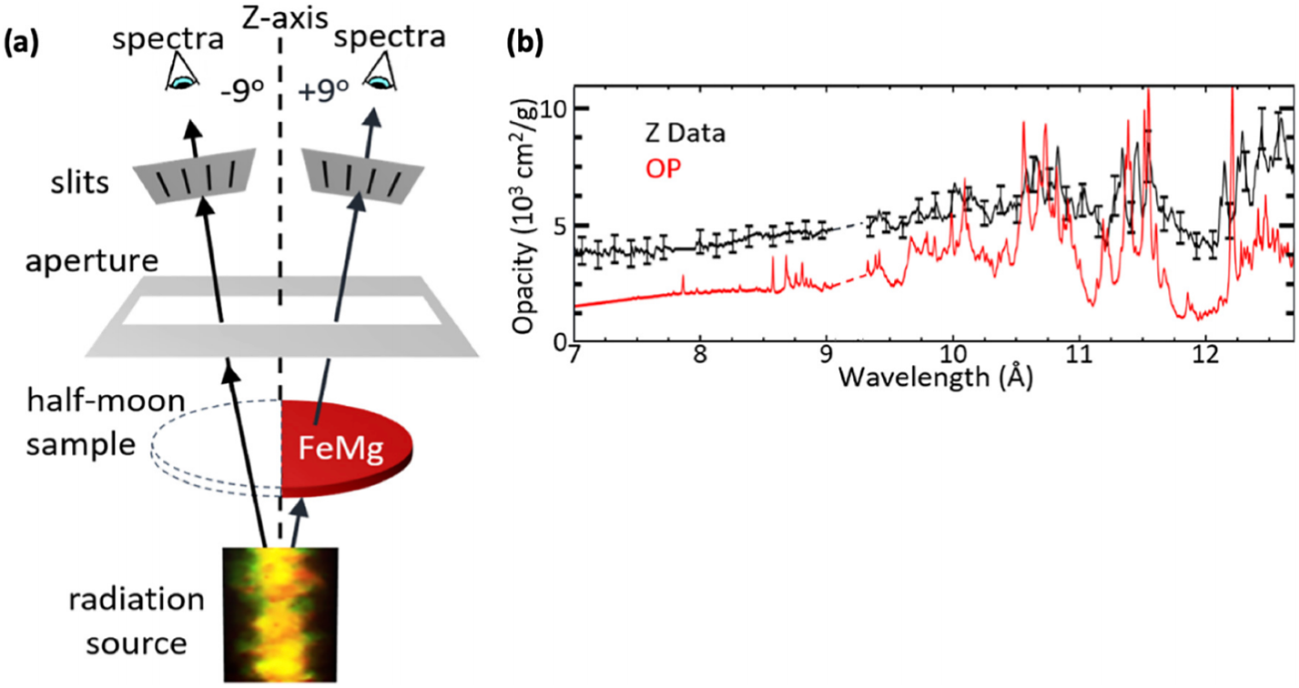
The higher-than-predicted iron opacity data account for about half the increase needed to resolve the Standard Solar Model discrepancy. However, the question remains: why are the model predictions lower than our measurements? This question is critical because, if the data are correct, our understanding of photon absorption in high-density matter must be revised. This would have far-reaching consequences for astrophysics and terrestrial science. For example, a widely used method to estimate stellar ages depends on opacity, and opacity revisions will therefore lead to substantial changes in age estimates. Furthermore, if solar composition, opacity, and helioseismology inferences are found to be consistent, the soundness of the Standard Solar Model will be reinforced, but the composition and opacity used to model other Sun-like stars must be revised. On the other hand, if observations and solar model inputs cannot be reconciled, possible modifications to the Standard Solar Model itself would be necessary. A new theory, for example, has been proposed to explain the enhanced opacity by taking account of two-photon absorption effect[Reference More, Hansen and Nagayama77].
Of course, the opacity is one of the most important elements to model stellar evolution. The consensus model for a classical nova invokes a binary star system, with accretion from a main-sequence star or evolved giant onto a WD due to Roche lobe overflow. As hydrogen-rich material is transferred to the WD through an accretion disk, the temperature at the base of the accreted envelope rises until it reaches 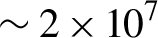 $\sim 2\times {10}^7$ K, at which point the accreted fuel undergoes fusion via the CNO cycle. A convective zone is born and grows until an optically thick wind is launched, giving rise to the observed classical nova. The launching of the optically thick wind is primarily due to the presence of the iron opacity bump. Accurate opacity of iron is essential to compare observation light cure to a theoretical model[Reference Rosenthal, Shen, Hallinan, Singh, Chomiuk, Margutti and Metzger78].
2.8 Photoionized plasma experiments
It is very challenging to study photoionized plasma, because it is hard to produce black-body radiation with radiation temperature more than 100 eV in laboratory to ionize very abundant atoms such as Si and Fe. However, such bright radiation sources in X-ray regime have been observed in the universe. The compact objects mean blackholes, neutron stars, and WDs, and a binary system is made of such a compact star and a normal star. The compact binary objects emit strong X-rays with which the property of the objects can be studied with use of the X-ray observation. To analyze the observed X-ray spectrum, modeling of photoionized plasma is essential and sophisticated codes have been developed. Such simulation codes should be verified and validated via comparison with appropriate experiments in the laboratory.
As high-Z ions emit X-ray line emissions, they are good targets to be observed to study the physics of very energetic radiation source. Cygnus X-1 and Cygnus X-3 are a well-known X-ray binary system[Reference Seward and Charles79]. They are located around 7.4 kpc (20,000 lightyears) away; however, they emit very luminous X-rays. A schematic of such a binary system is shown in Figure 28. The companion star is a massive normal star with very high-mass stellar wind to donate the matter to the compact object. As a compact object such as a blackhole absorbs the mass via strong gravitation, the matter of the accretion disc continuously falls into the blackhole. During the process of losing the angular momentum, the excess energy heats the matter and the matter near the compact object becomes extremely high-temperature plasma emitting almost Planckian radiation. The radiation temperature becomes almost 1 keV and the radiation photoionizes the accreting plasma.
A compact binary system. Strong X-ray from the accretion disc photoionizes the surface of a huge normal star[80].

How the plasma is strongly affected by photoionization in the atomic process is measured with the photoionization parameter  $\xi$ defined by
 \begin{align}\xi =\frac{L}{n_{\mathrm{e}}{R}^2}\left[\mathrm{erg}\cdot\mathrm{cm}^{-1}\cdot\mathrm{s}^{-1}\right],\end{align}
where  $L$ is the total luminosity of the compact object and
  $R$ is the radius of the most X-ray emitting plasma region of the accretion disc. The
  ${n}_{\mathrm{e}}$ is the electron density to measure the photorecombination. Equation (8) is a rough estimation of the ratio of the photoionization rate to the photorecombination rate. Note that the photoionization plasma is realized when the condition
  $\xi \gg 1$ is satisfied in the units of Equation (8).
A detailed analysis of the spectra from Cygnus X-3 has been performed[Reference Kallman, McCollough, Koljonen, Liedahl, Miller, Paerels, Pooley, Sako, Schulz, Trushkin and Corrales81]. The bright emission of He-like silicon K $\alpha$ line suggests the ionization parameter
 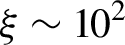 $\xi \sim {10}^2$ for the Cygnus 3 binary system. It is also concluded that the density must be higher than 10
 ${}^{12}$ cm
 ${}^{-3}$ in the region responsible for most of the emission. The electron temperature obtained from the energy balance relation is also calculated. It is about 20 eV at
  $\xi \sim {10}^2$. AGNs[Reference Kallman, McCollough, Koljonen, Liedahl, Miller, Paerels, Pooley, Sako, Schulz, Trushkin and Corrales81] extremely far from our galaxy are a strong X-ray source in the deep sky, and about 70% of X-rays observed far from our galaxy are inferred from many AGNs.
The photoionized plasmas are a model experiment of X-ray binary systems, whereas there are several differences owing to limit of laboratory plasma. One is the time dependence of atomic state of partially ionized atoms, the second is the expanding flow of plasma, and the third is optical depth especially of line radiation transport. Of course, the radiation source such as more than 1 keV radiation temperature is not yet possible in the laboratory. However, photoionized plasma itself is an interesting subject from the view point of the atomic process, opacity, line profile modeling, radiation transfer and so on.
Photoionized plasma has been studied to look for better coupling with the absorbing plasma in hohlraum targets, where laser energy is converted into radiation energy to be absorbed by fusion pellets in the hohlraum. In the NIF ignition campaign, almost Planckian radiation with radiation temperature 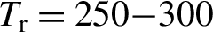 ${T}_{\mathrm{r}}=250{-}300$ eV has been used for implosions under the absorption of laser energy of 0.8–1.1 MJ[Reference Lindl, Landen, Edwards and Moses82]. The radiation continues for about 5 ns and it is expected that the photoionized plasma is almost in steady state. On the other hand, the Z-pinch machine is demonstrated to be an intense X-ray source and proposed to also be applicable to studying the physics of photoionized plasma in the universe[Reference Matzen83].
Preliminary design and experiments of photoionized plasma were reported for the cases with Z-pinch[Reference Bailey, Cohen, Chandler, Cuneo, Foord, Heeter, Jobe, Lake, Liedahl, MacFarlane, Nash, Nielson, Smelser and Stygar84] and laser-induced gold cavity[Reference Takabe16, Reference Morita, Nishimura, Ochi, Fujita, Fukao, Suzuki, Kawamura, Daido and Takabe85] radiations. The radiation temperature is in the rage of 80–200 eV. The absorption and emission spectra of such photoionized plasmas have been studied. In addition, scalability to very low-density plasmas in the universe was also discussed. Application of such photoionized experiments to astrophysics has been discussed internationally[Reference Mancini, Bailey, Hawley, Kallman, Witthoeft, Rose and Takabe86] and The Z Astrophysical Plasma Properties (ZAPP) collaboration has been initiated for applying the Z-pinch for a variety of astrophysical model experiments[Reference Rochau, Bailey, Falcon, Loisel, Nagayama, Mancini, Hall, Winget, Montgomery and Liedahl87].
Precise experimental results were first reported for Z-pinch photoionization plasma, where the Z-pinch radiation spectrum was observed and the radiation temperature was measured to be 165 eV[Reference Foord, Heeter, van Hoof, Thoe, Bailey, Cuneo, Chung, Liedahl, Fournier, Chandler, Jonauskas, Kisielius, Mix, Ramsbottom, Springer, Keenan, Rose and Goldstein88]. Charge distribution of photoionized iron plasma observed in the experiment is compared with three different atomic process codes including photoionization. Two of them are standard codes to analyze the photoionization plasma emission spectrum compared with X-ray satellite data, whereas the third is FLYCHK. It is clarified that charge distribution is insensitive to the iron plasma temperature for more than 150 eV under these experimental conditions. It is speculated that compared with AGN X-ray flux, the X-ray flux for contributing silicon photoionization is almost the same as that obtained by Z-pinch X-ray with  ${T}_{\mathrm{r}}=165$ eV[Reference Loisel, Bailey, Liedahl, Fontes, Kallman, Nagayama, Hansen, Rochau, Mancini and Lee89].
In order to relate such laboratory experiments to the binary system observations, higher radiation has been generated by use of radiation from an imploded spherical target. By use of the Gekko-XII laser system, 12 beams irradiate a target to generate almost 0.5 keV radiation temperature. Total energy of 4 kJ with pulse duration of 1.2 ns at green light (0.53  $\mu \mathrm{m}$) are impinged on a plastic target with the diameter 505
  $\mu \mathrm{m}$ and thickness 6.4
  $\mu \mathrm{m}$[Reference Fujioka, Takabe, Yamamoto, Salzmann, Wang, Nishimura, Li, Dong, Wang, Zhang, Rhee, Lee, Han, Tanabe, Fujiwara, Nakabayashi, Zhao, Zhang and Mima90]. Although the pulse duration of the radiation is 160 ps, it is enough to generate He-like silicon with the density
  ${n}_{\mathrm{e}}={10}^{20}$ cm
 ${}^{-3}$ located near the imploded core. Observation data from Cygnus X-3 and Vela X-1 are compared with the experimental data for the line emissions from He-like silicon[Reference Wang, Salzmann, Zhao, Takabe, Fujioka, Yamamoto, Nishimura and Zhang91]. The line inferred as the forbidden transitions only expected in low-density astrophysical plasma is also observed. However, time-dependent simulation for the experiment cannot reproduce this hump in spectrum. On the other hand, this hump is generated in computations in Ref. [Reference Wu, Duan, Li and Yan92], although the strength of three humps is not reproduced. This remains an open question.
The inter-combination line (1s ${}^2$
  ${}^1$S-1s2p
  ${}^3$P and 1s
 ${}^2$
  ${}^1$S-1s2p
  ${}^3$P) is strengthened by satellite lines from the Li-like species which has similar energies. Namely, 1s
 ${}^2$3p-1s2p3p transition has energy around 1.855 keV. These are known as satellite lines of Li-like ions.
Mancini et al. [Reference Mancini, Lockard, Mayes, Hall, Loisel, Bailey, Rochau, Abdallah, Golovkin and Liedahl93] have carried out sophisticated computer simulation with Boltzmann code for free electrons. The Boltzmann code is coupled with radiation hydrodynamic code. It is shown that photoexcitation is very important to control radiation cooling rate and the evaluated electron temperature is found to be lower than predicted by CLOUDY and XSTAR codes. In addition, the high-energy tail component generated by photoionization affects the population of the excited state enhancing the radiation cooling rate.
2.9 Blast waves of astrophysical explosions
Once a supernova explosion happens, the outward-going shock wave starts to propagate in the surrounding plasma while also heating the plasma. The heated plasma emits radiation of a wide range of photon energy. In Figure 29, the time evolution of radio emission of the expanding shell formed by supernova SN1993J is shown between May 1993 (top left) and February 2000 (bottom right)[Reference Bartel94]. During the explosive death of a large star, the outer layers are propelled outwards as the collapsing core rebounds. This supernova was discovered on 28 March 1993. It is around 11 million lightyears distant, in the constellation Ursa Major. Its relative closeness allows observation by radio interferometry with arrays such as the Very Large Array (VLA) and the Very Long Baseline Array (VLBA). The expansion has decelerated from 16,000 to 10,000 km/s.
Time evolution of radio emission after the explosion of SN1993J[Reference Bartel94].

A long-time evolution of the hydrodynamics after an explosion of a supernova is modeled by a Sedov–Taylor blast wave as a self-similar solution. However, it is the case of a simplified solution of the hydrodynamic equation with a central singular explosion source. It is known that the radiation cooling induces the shock front instability, known as Vishiniac instability. It is said that the turbulent image of Tyco SNR is due to such instability. A model experiment of the instability was performed with laser blast wave a long time ago[Reference Grun, Laming, Manka, Donnelly, Covington, Fischer, Velikovich and Khokhlov95]. A more precise experiment has been performed to compare with the theoretical growth rate of the instability[Reference Edens, Ditmire, Hansen, Edwards, Adams, Rambo, Ruggles, Smith, Porter and Kyrala96], and also on the stability of the bow shock[Reference Suzuki-Vidal, Lebedev, Ciardi, Pickworth, Rodriguez, Gil, Espinosa, Hartigan, Swadling, Skidmore, Hall, Bennett, Bland, Burdiak, de Grouchy, Music, Suttle, Hansen and Frank18].
Optical imaging of blast waves and accompanying shocks has been developed to investigate the blast wave dynamics[Reference Tubman, Scott, Doyle, Meinecke, Ahmed, Alraddadi, Bolis, Cross, Crowston, Doria, Lamb, Reville, Robinson, Tzeferacos, Borghesi, Gregori and Woolsey97]. Thanks to XFEL facilities, it is now also possible to obtain the image of shock waves propagating into solid materials[Reference Schropp, Hoppe, Meier, Patommel, Seiboth, Ping, Hicks, Beckwith, Collins, Higginbotham, Wark, Lee, Nagler, Galtier, Arnold, Zastrau, Hastings and Schroer70]. The advancement of imaging technology is very important to study, for example, the collision of two blast waves[Reference Albertazzi, Mabey, Michel, Rigon, Marquès, Pikuz, Ryazantsev, Falize, Van Box Som, Meinecke, Ozaki, Ciardi, Gregori and Koenig98] and the effect of an external magnetic field on the dynamics of blast waves[Reference Takahashi99]. A radiative blast wave is also studied and compared with simulation[Reference Koenig, Michel, Yurchak, Michaut, Albertazzi, Laffite, Falize, Van Box Som, Sakawa, Sano, Hara, Morita, Kuramitsu, Barroso, Pelka, Gregori, Kodama, Ozaki, Lamb and Tzeferacos100].
Collision of shocks and clumpy matter such as a molecular cloud in space triggers star formation via active gravitation interaction after the collision. As we see, for example, in Ref. [Reference Kuranz, Park, Huntington, Miles, Remington, Plewa, Trantham, Robey, Shvarts, Shimony, Raman, MacLaren, Wan, Doss, Kline, Flippo, Malamud, Handy, Prisbrey, Krauland, Klein, Harding, Wallace, Grosskopf, Marion, Kalantar, Giraldez and Drake101], shock and clump interactions generate vortex motion to form a complicated density distribution after the shock impact. A good example of the vortex formation is hydrodynamic instability. An X-ray backlight method has been developed to obtain a clear image of dense plasma hydrodynamics. The growth of the instability due to the vortices generated by the passage of a shock wave is shown in Figure 30. Such a micro shock tube and X-ray backlight technique is a very powerful method to study the physics of shock–matter interaction in the laboratory.
A micro shock tube with X-ray backlight diagnostics in a multibeam laser facility. Richtmyer–Meshkov instability growth is measured on the right by X-ray exposure[Reference Kuranz, Park, Huntington, Miles, Remington, Plewa, Trantham, Robey, Shvarts, Shimony, Raman, MacLaren, Wan, Doss, Kline, Flippo, Malamud, Handy, Prisbrey, Krauland, Klein, Harding, Wallace, Grosskopf, Marion, Kalantar, Giraldez and Drake101].

It should be noted that controlled high explosion is used to study the hydrodynamic instability driven by blast wave passage[Reference Musci, Petter, Pathikonda, Ochs and Ranjan102]. The size of gases is around 20 cm, much larger than the laser micro shock tube of about 1 mm. The instability is initiated by passing a Taylor–Sedov blast wave originating from a controlled detonation through a perturbed and stably stratified interface between two gases. The large ensembles of time-resolved Mie scattering imaging have been measured. The analysis has been performed on the instability evolution between different gas pairs to demonstrate the wide range of development and turbulent behavior that may occur between different supernova layers.
Plasma jet formation and its application to astrophysical jets have been studied since the early days. The laboratory experiments of a well-collimated radiative jet with high Mach number has been successfully created to mimic the evolution of Herbig–Haro (HH) objects[Reference Yuan, Li, Tao, Wei, Zhong, Zhu, Li, Zhao, Li, Han, Zhang, Liang, Wang, Hu, Zheng, Jiang, Du, Ding, Zhou, Zhu, Zhu, Zhao and Zhang103]. It was found that the radiation cooling effect within the jet and the outer rare surrounding plasmas from the X-ray ( $>$keV) photoionized target contribute to the jet collimation. The local nonuniform density structures along the collimated radiative jet axis are caused by the pressure competition between the inner jet and the outer plasmas.
On the other hand, such jets were placed in a custom-designed solenoid capable of generating field strengths up to 5 T[Reference Manuel, Kuranz, Rasmus, Klein, MacDonald, Trantham, Fein, Belancourt, Young, Keiter, Drake, Pollock, Park, Hazi, Williams and Chen104]. Proton radiographs of the well-characterized B-field, without a plasma jet, suggested an external source of trapped electrons that affects proton trajectories. The background magnetic field was aligned with the jet propagation direction, as is the case in many astrophysical systems. Optical interferometry showed that magnetization of the plasma results in disruption of the collimated flow and instead produces a hollow cavity. This result is a topic of ongoing investigation.
2.10 Hydrodynamic instability and turbulent mixing
As mentioned in the introduction, hydrodynamic instability was the first bridge between astrophysical plasma and laser-produced plasma. When the material mixing in the supernova SN1987A explosion was found by X-ray satellite, the hydrodynamic instability of fusion capsule implosion had been studied intensively as the most critical physics preventing the spherically symmetric implosion dynamics. The hydrodynamic instability and resultant turbulent mixing have been studied for a three-dimensional core-collapse system with computing in astrophysics[Reference Burrows, Radice and Vartanyan13] and theoretically, computationally, and experimentally mainly in laser plasma as reviewed in Ref. [Reference Zhou, Clark, Clark, Glendinning, Skinner, Huntington, Hurricane, Dimits and Remington105].
Shock waves generate vortices in nonuniform fluids and plasmas. The vortex generation in plasmas directly relates to hydrodynamic instabilities. It is easily understood by the equation for vortex  $\overrightarrow{\omega}$
  $\left(=\nabla \times \overrightarrow{v}\right)$:
 \begin{align}\frac{\partial \overrightarrow{\omega}}{\partial t}=\nabla \times \left(\overrightarrow{u}\times \overrightarrow{\omega}\right)+\frac{\nabla \rho \times \nabla P}{\rho^2}+\frac{4}{3}v{\nabla}^2\overrightarrow{\omega}.\end{align}
In Equation (9), the second term on the right-hand side, the vector product of the gradients of density and pressure, is the source term to generate vortices. This term is called the baroclinic effect and is well known as the source to generate vortices in the Earth’s atmosphere, which finally become a typhoon or hurricane. In laser fusion and related areas, it is known as the source term of hydrodynamic instability such as Rayleigh–Taylor and Richtmyer–Meshkov instabilities and it is easy to see the physics intuitively[Reference Jameson and Takabe106].
It is informative to note the following similarity between Equations (2) and (9). The vortex is the rotation of the velocity and directly related to the vortex motion of electron fluids in the case of plasma,  $\omega \iff B$. This is seen as the same form of the first terms in the right-hand side of Equations (9) and (2), namely the convection term. The third term in Equation (9) and the second term in Equation (2) are diffusion terms. Then, the second term in Equation (9) and the last term in Equation (2) are the source terms. This means that when hydrodynamic instabilities are induced in plasma fluids, the magnetic field is also generated in general.
A supernova’s explosion is driven by a blast wave. It also induces Rayleigh–Taylor and Richtmyer–Meshkov instabilities. These instabilities cause strong mixing of matter in a progenitor star. Such mixing is inferred to be the reason for early observation of heavy mass elements synthesized in the star before its explosion[Reference Abarzhi, Bhowmick, Naveh, Pandian, Swisher, Stellingwerf and Arnett107].
Time evolution of a core-collapse supernova is shown in Figure 31[Reference Janka, Alsabti and Murdin108]. Owing to the core collapse at  $t=0$, a proto-neutron star is formed at the center and huge number of neutrinos are emitted with total energy of about 10
 ${}^{53}$ erg. In the case of one-dimensional simulation, the absorbed neutrino energy is not enough to explode the star and the shock wave disappears because of endothermic nuclear reaction. In multidimensional simulations, it is found that the neutrino efficiently heats due to the mixing effect, and the matter can obtain enough energy to maintain the outgoing shock wave, and the system explodes as shown in Figure 32.
Time evolution of the neutrino-driven explosion of a 15M star as obtained in a multidimensional hydrodynamic simulation, visualized by a mass-shell plot. The star collapses at t = 0 to generate a shock wave. The shock is powered by neutrino heating[Reference Janka, Alsabti and Murdin108].

A three-dimensional explosion simulation at about 0.5 s after the core ignited. The bluish, almost transparent surface is the shock front with an average radius of 1900 km (MPA)[Reference Janka, Alsabti and Murdin108].

Soon after the collapse, the shock wave accelerates the matter and low-density region appears behind. This density profile is unstable against the gravity and the Rayleigh–Taylor instability becomes important. Owing to the deformation behind the shock, the neutrinos can keep being absorbed by relatively low-temperature materials. Therefore, the mixing helps to enhance the absorption of neutrinos after  $t=200$ ms in Figure 31. Thus, the mixing is the key issue for supernovae to be able to explode.
It is noted that a more precise mixing model is required even in three-dimensional simulation. Turbulent mixing has not been modeled in supernova simulation so far, although it is important to advance the supernova explosion model. In fact, in the radiation-driven fusion experiment with NIF, it is reported that the mixing of fuel and capsule materials is important and degrades the neutron yields drastically[Reference Ma, Patel, Izumi, Springer, Key, Atherton, Barrios, Benedetti, Bionta, Bond, Bradley, Caggiano, Callahan, Casey, Celliers, Cerjan, Church, Clark, Dewald, Dittrich, Dixit, Döppner, Dylla-Spears, Edgell, Epstein, Field, Fittinghoff, Frenje, Johnson, Glenn, Glenzer, Grim, Guler, Haan, Hammel, Hatarik, Herrmann, Hicks, Hinkel, Hopkins, Hsing, Hurricane, Jones, Kauffman, Khan, Kilkenny, Kline, Kozioziemski, Kritcher, Kyrala, Landen, Lindl, Le Pape, MacGowan, Mackinnon, MacPhee, Meezan, Merrill, Moody, Moses, Nagel, Nikroo, Pak, Parham, Park, Ralph, Regan, Remington, Robey, Rosen, Rygg, Ross, Salmonson, Sater, Sayre, Schneider, Shaughnessy, Sio, Spears, Smalyuk, Suter, Tommasini, Town, Volegov, Wan, Weber, Widmann, Wilde, Yeamans and Edwards109, Reference Zylstra, Casey, Kritcher, Pickworth, Bachmann, Baker, Biener, Braun, Clark, Geppert-Kleinrath, Hohenberger, Kong, Le Pape, Nikroo, Rice, Rubery, Stadermann, Strozzi, Thomas, Volegov, Weber, Wild, Wilde, Callahan and Hurricane110]. As shown in Figure 33, a clear correlation can be seen between the decrease of neutron yields and radiation emission stemming from the mixed and heated atoms from the capsule material. It is reasonable to conclude that the mixing of atomic scale in the compressed and heated DT fuel plasma prevents the final increase of the fuel temperature by the pressure work. This is the most critical issue of the inertial confinement fusion concept.
DT neutron yield versus measured X-ray enhancement ratio for the layered low-foot (blue) and high-foot (green) laser implosions with NIF[Reference Ma, Patel, Izumi, Springer, Key, Atherton, Barrios, Benedetti, Bionta, Bond, Bradley, Caggiano, Callahan, Casey, Celliers, Cerjan, Church, Clark, Dewald, Dittrich, Dixit, Döppner, Dylla-Spears, Edgell, Epstein, Field, Fittinghoff, Frenje, Johnson, Glenn, Glenzer, Grim, Guler, Haan, Hammel, Hatarik, Herrmann, Hicks, Hinkel, Hopkins, Hsing, Hurricane, Jones, Kauffman, Khan, Kilkenny, Kline, Kozioziemski, Kritcher, Kyrala, Landen, Lindl, Le Pape, MacGowan, Mackinnon, MacPhee, Meezan, Merrill, Moody, Moses, Nagel, Nikroo, Pak, Parham, Park, Ralph, Regan, Remington, Robey, Rosen, Rygg, Ross, Salmonson, Sater, Sayre, Schneider, Shaughnessy, Sio, Spears, Smalyuk, Suter, Tommasini, Town, Volegov, Wan, Weber, Widmann, Wilde, Yeamans and Edwards109].

3 Cosmic-ray acceleration by wakefields
3.1 Introduction
The origins of comic rays have been a long-standing unsolved problem since the discovery of cosmic rays in the last century. More than half a century ago, Enrico Fermi proposed his unique idea for the acceleration of cosmic rays by moving magnetic clouds (Fermi acceleration)[Reference Fermi111]. His original idea could not explain the observed cosmic-ray spectra with nonthermal, power-law components up to very high energies; however, this was overcome with the applications of the Fermi acceleration to a collisionless shock. In the presence of a collisionless shock, energetic particles or cosmic rays are efficiently accelerated by the first-order Fermi acceleration or the so-called DSA[Reference Bell112, Reference Blandford and Ostriker113], where the energy spectra of the accelerated particles naturally show power-law dependence. The most eminent feature of the DSA is the universality; in the presence of strong shock waves, and this is often the case in the universe, the spectral index is  $-2$ independent of the plasma and shock parameters. Taking into account the transport effects from the acceleration sites to the Earth, it is widely believed that the DSA explains the observed cosmic-ray spectra. It is widely believed that the galactic cosmic rays are accelerated by the DSA associated with nonrelativistic collisionless shocks in SNRs. Therefore, a collisionless shock also has central importance in cosmic-ray research.
Although the DSA is considered to be a standard acceleration mechanism of cosmic rays within our galaxy, the origin of extragalactic cosmic rays has been an open unsolved problem. It is known that the cosmic-ray spectrum changes its slope at  ${E}_{\mathrm{cr}}\sim 15.5$, the so-called knee energy, and it is widely accepted that the galactic cosmic rays are accelerated by the DSA at SNRs[Reference Swordy114]. It is still open how and where the cosmic rays beyond the knee energies are accelerated; however, at least the UHECRs are considered to be from oustside our galaxy because their gyro radii are much larger than the size of galaxy. A possible candidate of the cosmic-ray acceleration is the wakefield acceleration in extreme astrophysical conditions[Reference Iwamoto, Amano, Hoshino, Matsumoto, Niemiec, Ligorini, Kobzar and Pohl57, Reference Takahashi, Hillman, Tajima, Tajima, Mima and Baldis115–Reference Mizuta, Ebisuzaki, Tajima and Nagataki126]. Wakefield acceleration was first proposed in laboratory plasmas[Reference Tajima and Dawson127], and its developments and applications can be found in a recent review[Reference Tajima, Yan and Ebisuzaki128]. In the laser wakefield acceleration, the strong ponderomotive force of an intense laser pulse expels electrons in a plasma, resulting in the formation of space charge or an electrostatic wakefield. This is analogous to the wake created by a ship on the water, where the ship expels water on the pass. The perturbations on the electron density can propagate as a fundamental electron plasma wave or Langmuir wave. The phase velocity of the wakefield is equal to the group velocity of the laser pulse, which is again analogous to that the phase of the first wake on the water propagates with the ship. Therefore, the wakefields in laser-produced plasmas propagate at a velocity close to the speed of light; once the electrons are injected into the wakefield, they can be quickly accelerated to relativistic energies.
The wakefield acceleration was first applied to cosmic-ray acceleration in Ref. [Reference Chen, Tajima and Takahashi116], where Alfvén wave or Alfvén shock is considered. Purely stochastic assumption results in the power-law energy distribution function with an index of –2[Reference Chen, Tajima and Takahashi116], which is equivalent to the DSA. The wakefield acceleration is longitudinal to the particle motion, that is, synchrotron or cyclotron emission is irrelevant[Reference Chen, Tajima and Takahashi116], which is inevitable in the DSA. Dieckmann et al. discussed the wakefield induced by relativistic plasma flow in the relativistic shock upstream with one-dimensional PIC simulations[Reference Dieckmann, Shukla and Eliasson118]. The wakefield excitation by whistler waves has been discussed analytically as well as numerically with one-dimensional PIC simulation[Reference Chang, Chen, Lin, Noble and Sydora121, Reference Chen, Chang, Lin, Noble and Sydora122]. The wakefield excited by Alfvén wave in the relativistic jet from an accreting supermassive blackhole has been discussed analytically[Reference Ebisuzaki and Tajima123], and the excitation of Alfvén waves has been confirmed with three-dimensional general relativistic magnetohydrodynamic simulations[Reference Mizuta, Ebisuzaki, Tajima and Nagataki126]. Lyubarsky[Reference Lyubarsky117] and Hoshino[Reference Hoshino119] considered the intense electromagnetic or light waves as precursor waves in relativistic magnetized shocks, which can induce a wakefield using one-dimensional PIC simulations. Iwamoto et al. extended the one-dimensional model to two dimensions to address the multidimensionality of the precursor wave propagations[Reference Iwamoto, Amano, Hoshino, Matsumoto, Niemiec, Ligorini, Kobzar and Pohl57, Reference Iwamoto, Amano, Hoshino and Matsumoto124, Reference Iwamoto, Amano, Hoshino and Matsumoto125]. By focusing on the wakefield acceleration upstream, we have shown the universality of the power-law acceleration by a turbulent wakefield with two-dimensional PIC simulations[Reference Kuramitsu, Sakawa, Kato, Takabe and Hoshino120, Reference Kuramitsu, Sakawa, Hoshino, Chen and Takabe129–Reference Liu, Isayama, Chen and Kuramitsu131]. Most of the acceleration models mentioned previously can account for the origin of UHECRs with energies of approximately  ${10}^{20}$ eV or more. However, it is hard to confirm the acceleration scenarios with astrophysical observations. An alternative approach to verify the acceleration models is laboratory experiment with intense lasers. In this section, we consider the precursor electromagnetic waves in the astrophysical collisionless shock discussed in Ref. [Reference Hoshino119] and possible verification of the model in the laboratories[Reference Kuramitsu, Sakawa, Kato, Takabe and Hoshino120, Reference Kuramitsu, Nakanii, Kondo, Sakawa, Mori, Miura, Tsuji, Kimura, Fukumochi, Kashihara, Tanimoto, Nakamura, Ishikura, Takeda, Tampo, Kodama, Kitagawa, Mima, Tanaka, Hoshino and Takabe132, Reference Kuramitsu, Nakanii, Kondo, Sakawa, Mori, Miura, Tsuji, Kimura, Fukumochi, Kashihara, Tanimoto, Nakamura, Ishikura, Takeda, Tampo, Kodama, Kitagawa, Mima, Tanaka, Hoshino and Takabe133].
3.2 Wakefield generation and acceleration in relativistic collisionless shocks
In this section, we briefly review Hoshino’s model where PIC simulations show the efficient particle acceleration by the wakefield acceleration in the presence of a perpendicular relativistic collisionless shock[Reference Hoshino119]. Figure 34 shows the results from the one-dimensional PIC simulation, where the shock front is located at  $X\sim -400$, indicating the sharp transition of ion and electron velocity components. In the relativistic perpendicular collisionless shock, the incoming plasma electrons interacting with the shocked magnetic field radiate large amplitude electromagnetic (light) waves (
 ${B}_z$) via the synchrotron maser instability[Reference Hoshino, Arons, Gallant and Langdon134], which can propagate toward the upstream of the shock (
 $X<-400$). The ponderomotive force of the light waves excites the wakefield (
 ${E}_x$), and the wakefield accelerates the upstream electrons and also ions. Note that the DSA requires the particles to be repeatedly scattered back and forth of the shock front; however, the wakefield acceleration operates upstream.
The spatial transitions of physical quantities are plotted: from top to bottom, the  $x$- and
  $y$-components of ion velocity, the
  $x$- and
  $y$-components of electron velocity, the
  $x$-component of electric field corresponding to the wakefield, and the
  $z$-component of magnetic field corresponding to the light precursor waves[Reference Hoshino119].

The spatial and temporal scales of a relativistic collisionless shock are vast compared with the plasma scale lengths. There are two important parameters governing the wakefield acceleration in the astrophysical conditions: the normalized wave amplitude  ${a}_0$ and the frequency ratio between the plasma and the light
  ${\omega}_{\mathrm{p}}/{\omega}_{\mathrm{L}}$. From the simulation
  ${\omega}_{\mathrm{p}}/{\omega}_{\mathrm{L}}{\sim}1/3$–1/2 and
  ${a}_0\sim {\gamma}_1$, where
  ${\gamma}_1$ is the Lorentz factor of upstream flow energy. The Lorentz factors of AGN jets and GRBs are
  ${\gamma}_1\sim 10$ and approximately 100–1000, respectively, and, therefore, there must be intense light waves in the upstream of such extreme relativistic phenomena in the universe. One may argue that in the one-dimensional system all the wave modes propagate in the same direction; in reality, in multidimensions the precursor light waves may propagate in arbitrary direction. This leads to the lower wave amplitude and inefficient wakefield excitation.
To address the multidimensionality of the precursor light propagations, Iwamoto et al. have performed two-dimensional PIC simulations of relativistic shocks in electron–positron pair plasmas and electron–ion plasmas[Reference Iwamoto, Amano, Hoshino, Matsumoto, Niemiec, Ligorini, Kobzar and Pohl57, Reference Iwamoto, Amano, Hoshino and Matsumoto124, Reference Iwamoto, Amano, Hoshino and Matsumoto125]. Figure 35 shows the relativistic perpendicular shock in a pair plasma in the presence of relatively strong magnetic field[Reference Iwamoto, Amano, Hoshino and Matsumoto124], where the downstream is located on the left-hand side of the simulation box in contrast to Figure 34. Note that in a pair plasma, there is no Langmuir wave because the electron and positron have the same mass; there is no wakefield acceleration in the pair plasma. Nevertheless, what they focus on here is the large amplitude precursor wave excitation even in the two-dimensional PIC simulations. Owing to the strong ponderomotive force of the precursor waves, there are strong density fluctuations seen in the upstream of the shock (see the top panel of Figure 35). These filamentary structures are considered to be excited via the filamentation instability, and to act as a wave guide. This can be one of the reasons why the precursor waves can be such large amplitude even in two dimensions. When the background magnetic field is relatively weak, the Weibel instability is operative. They also investigated the competition between the synchrotron maser instability and the Weibel instability and showed that the precursor waves coexisted in the presence of the Weibel instability[Reference Iwamoto, Amano, Hoshino and Matsumoto124] (not shown here). They also showed that the Weibel instability could enhance the precursor waves[Reference Iwamoto, Amano, Hoshino and Matsumoto125] (not shown here).
Large-amplitude precursor waves can be excited in the relativistic collisionless shock even in multidimensions. Iwamoto et al. have further extended their study in electron–ion plasmas, where the wakefield can be excited and, thus, the wakefield acceleration takes place. Figure 36 shows a similar plot to Figure 35 but in an electron–ion plasma with much larger computer resources[Reference Iwamoto, Amano, Hoshino, Matsumoto, Niemiec, Ligorini, Kobzar and Pohl57]. In Figure 36, the precursor waves in  ${B}_z$ are clearly seen as expected from the simulation results in Refs. [Reference Iwamoto, Amano, Hoshino and Matsumoto124,Reference Iwamoto, Amano, Hoshino and Matsumoto125]. As also expected, in an electron–ion plasma the wakefield
  ${E}_x$ is excited and the electron and ion heating can be seen in the upstream in Figure 36.
Relativistic perpendicular collisionless shock in a pair plasma: from top to bottom, electron density ( ${N}_{\mathrm{e}}$), the electron density averaged over
  $y$ direction (
 $\langle{N}_{\mathrm{e}}\rangle$), the
  $z$ component of magnetic field corresponding to the precursor waves (
 ${B}_z$), the line profile of
  ${B}_z,$ the
  $x$ component of electric field averaged over
  $y$ direction corresponding to the wakefield
  $\left(\langle{E}_x\rangle\right)$, and the
  $x$ and
  $y$ components of electron velocity. The shock front is located at
  $x\sim 280$[Reference Iwamoto, Amano, Hoshino and Matsumoto124].

Relativistic perpendicular collisionless shock in an electron–ion plasma: from top to bottom, the  $z$ component of the magnetic field corresponding to the precursor waves (
 ${B}_z$), the line profile of
  ${B}_z$, the
  $x$ component of the electric field corresponding to the wakefield (
 ${E}_x$), the averaged
  ${E}_x$ over
  $y$ direction (
 $\langle{E}_x\rangle$), and the
  $x$ components of electron and ion velocities. The shock front is located at
  $x\sim 1100$[Reference Iwamoto, Amano, Hoshino, Matsumoto, Niemiec, Ligorini, Kobzar and Pohl57].

Figure 37 shows the precursor wave energies against the electron magnetization parameter from the one-dimensional (blue) and two-dimensional PIC simulations (red) in pair plasmas (solids lines; rescaled shown as dashed lines) and in electron–ion plasmas (open circles). The electron magnetization parameter is the ratio between the magnetic field energy and the electron kinetic energy, defined as  ${\sigma}_{\mathrm{e}}\equiv {B}_1^2/\left(4{\pi \gamma}_1{N}_1{m}_{\mathrm{e}}{c}^2\right)={\omega}_{\mathrm{ce}}^2/{\omega}_{\mathrm{pe}}^2$, where
  ${B}_1$,
  ${\gamma}_1$ and
  ${N}_1$ are the magnetic field strength, bulk Lorentz factor and the electron number density upstream, respectively,
  ${m}_{\mathrm{e}}$ is the electron mass,
  $c$ is the speed of light, and
  ${\omega}_{\mathrm{ce}}$ and
  ${\omega}_{\mathrm{pe}}$ are the proper electron cyclotron and plasma frequencies, respectively. The
  ${\sigma}_{\mathrm{e}}$ parameter is a major governing parameter of relativistic shock dynamics. Although the precursor wave energies in two-dimensional PIC simulations are about one to two orders of magnitude lower than those in one dimension in a wide range of
  ${\sigma}_{\mathrm{e}}$, it is considered that the precursor waves are still intense in high-energy astrophysical phenomena because
  ${a}_0\propto {\gamma}_1$. Let us recall that there are a number of relativistic shocks, for instance, in ANG jets, gamma-ray bursts, and pulsar winds with
  ${\gamma}_1\sim \mathrm{10,100}-1000,$ and
  ${10}^{6}{-}10^{7}$, respectively.
The precursor wave energies are plotted in terms of the magnetization parameter from various simulation runs[Reference Iwamoto, Amano, Hoshino, Matsumoto, Niemiec, Ligorini, Kobzar and Pohl57].

Figure 38 shows the energy spectra of electrons evaluated at the upstream rest frame to compare with our upstream model in numerical computations and in laboratory experiments[Reference Kuramitsu, Sakawa, Kato, Takabe and Hoshino120, Reference Kuramitsu, Sakawa, Hoshino, Chen and Takabe129–Reference Kuramitsu, Nakanii, Kondo, Sakawa, Mori, Miura, Tsuji, Kimura, Fukumochi, Kashihara, Tanimoto, Nakamura, Ishikura, Takeda, Tampo, Kodama, Kitagawa, Mima, Tanaka, Hoshino and Takabe133, Reference Liu, Kuramitsu, Isayama and Chen135]. It is clearly shown that the nonthermal electron and ion acceleration (except for ions with  ${\sigma}_{\mathrm{e}}=0.1$) and the spectra are well represented with a power law with an index of –2, consistent with our numerical and experimental results also shown in the following.
Energy spectra of electrons in the upstream rest frame shown in both logarithmic scales[Reference Iwamoto, Amano, Hoshino, Matsumoto, Niemiec, Ligorini, Kobzar and Pohl57].

3.3 Wakefield acceleration in upstream and the model experiment
In this section, we briefly review our numerical simulations[Reference Kuramitsu, Sakawa, Kato, Takabe and Hoshino120] and laboratory simulations[Reference Kuramitsu, Nakanii, Kondo, Sakawa, Mori, Miura, Tsuji, Kimura, Fukumochi, Kashihara, Tanimoto, Nakamura, Ishikura, Takeda, Tampo, Kodama, Kitagawa, Mima, Tanaka, Hoshino and Takabe132, Reference Kuramitsu, Nakanii, Kondo, Sakawa, Mori, Miura, Tsuji, Kimura, Fukumochi, Kashihara, Tanimoto, Nakamura, Ishikura, Takeda, Tampo, Kodama, Kitagawa, Mima, Tanaka, Hoshino and Takabe133] of the cosmic-ray acceleration by wakefield. In the relativistic perpendicular collisionless shocks, the precursor light waves excited via the synchrotron maser instability propagate toward the upstream as shown in the previous section. The precursor waves have much larger spatial scales than the electron scales because the astrophysical shocks are much larger than the electron scales. We focused on the wakefield excitation and the electron acceleration in the upstream because it is still difficult to experimentally simulate the relativistic shocks. By performing two-dimensional PIC simulations, a model experiment of cosmic-ray acceleration by the wakefield induced by an intense laser pulse was proposed, where the laser pulse is substituted for the large-amplitude precursor light waves in the astrophysical shocks[Reference Kuramitsu, Sakawa, Kato, Takabe and Hoshino120]. Here the background magnetic field does not take into account that the background magnetic field is essential for the precursor excitations, however, it causes minor effects in the wakefield acceleration. We have numerically investigated the effects of magnetic fields and shown that the power-law spectrum with an index of –2 is universally produced even in the presence of the background magnetic fields[Reference Liu, Isayama, Chen and Kuramitsu131] (not shown here).
Figure 39 shows the time evolutions of the wakefield acceleration, where an intense light (laser) pulse with larger spatial scale than the electron plasma wavelength propagates in an underdense plasma. At the early time in left panels, relatively coherent wakefield is excited in Figure 39(g) as the intense ponderomotive force of the laser pulse in Figure 39(a) expels the electrons as in Figure 39(d). One can see the longitudinal modulation in the laser electric field in Figure 39(a) due to the back reaction of wakefield excitation. In the center panels in later time, the longitudinal modulation is more eminent, and the traverse modulation can be seen in the leading edge of the pulse and behind. This is also seen in the density fluctuations (Figure 39(e)) and equivalently in the wakefield (Figure 39(h)). Further as time passes in the right panels, the light is more filamented and modulated in Figure 39(c), resulting in more incoherent density structure (Figure 39(f)) or turbulent wakefield (Figure 39(i)). The acceleration can take place in each wake: multiple injections and accelerations are evident in Figures 39(j)–39(l). The acceleration is nonthermal from the earlier time (Figure 39(m)) and clearly shows the power-law acceleration with an index of –2 in Figures 39(n) and 39(o). It is known that a laser pulse with larger spatial and temporal scales than the electron plasma wave scale is self-organized to have a comparable scale to the plasma wavelength via the self-modulation and the filamentation. As the modulated and filamented part of the light wave can excite the wakefield, a large-scale laser pulse can be regarded as part of the light precursor waves in the astrophysical shocks.
Wakefield acceleration due to an intense laser pulse with large spatial scale in a plasma: (a)–(c) the laser electric field, (d)–(f) the electron number density, and (g)–(i) the wakefield are shown in two-dimensional space; (j)–(l) the electron momenta in the direction parallel to the laser propagation ( $x$)
$x$)  ${p}_x$ are shown in terms of
  $x$; (m)–(o) the energy distribution functions of electrons are plotted in both logarithmic scales. The time passes from left to right panels[Reference Kuramitsu, Sakawa, Kato, Takabe and Hoshino120].

As mentioned in the introduction, a power law with an index of –2 is significant in astrophysics, because the index of cosmic-ray spectra is considered to be –2 and the DSA explains this well independently of plasma and shock parameters as long as the shock is strong. The universality of the wakefield acceleration has been investigated analytically and numerically in various conditions[Reference Kuramitsu, Sakawa, Kato, Takabe and Hoshino120, Reference Kuramitsu, Sakawa, Hoshino, Chen and Takabe129–Reference Liu, Isayama, Chen and Kuramitsu131, Reference Liu, Kuramitsu, Isayama and Chen135]. Figure 40 shows the energy distribution functions of electrons by changing the two governing parameters in astrophysical conditions as well as the pulse shape, which is also a governing parameter in the laboratory wakefield acceleration[Reference Kuramitsu, Sakawa, Kato, Takabe and Hoshino120]. The self-modulation and filamentation can make the wakefield turbulent, and in such a field the electrons are nonthermally accelerated, resulting in a power-law energy spectra with an index of approximately  $-2$ independent of the laser and the plasma conditions as long as the laser intensity is relativistic[Reference Kuramitsu, Sakawa, Kato, Takabe and Hoshino120, Reference Kuramitsu, Sakawa, Hoshino, Chen and Takabe129], which are the cases of the light waves excited in the astrophysical shock environments. The power-law spectrum with an index of –2 owing to the turbulent wakefield is also universal. Furthermore, as discussed in the introduction there is no energy loss by synchrotron emissions because the wakefield acceleration is longitudinal[Reference Chen, Tajima and Takahashi116]. Importantly, this model can be proved by laboratory experiments; only the current and the future laser facilities can provide such strong light sources. Laboratory astrophysics provides an alternative, experimental approach to study high-energy phenomena in the universe.
Electron energy distribution functions show power-law spectra with an index of –2 independent of (a) the normalized vector potential, (b) frequency ratio between plasma and laser frequency, and (c) the pulse shape[Reference Kuramitsu, Sakawa, Hoshino, Chen and Takabe129].

Ever since the discovery of cosmic rays, a number of scientists in space physics, astrophysics and plasma physics have intensively and extensively investigated the origins of the cosmic rays for a century. However, on the mechanism of the extragalactic cosmic-ray acceleration, only analytic and numerical investigations have been carried out and there is no way to prove them by observations. Our approach is entirely different from the conventional space and astrophysical plasma physics; scaled laboratory experiments with an intense laser pulse are performed to prove the acceleration model. There are two important governing parameters in the wakefield acceleration, the normalized wave amplitude and the ratio between plasma and light frequency, and the numerical simulations predict the universality of the wakefield acceleration as shown previously.
Figure 41(a) shows the schematic image of the experiment; the preformed plasma is created with the implosion of cylinder by Gekko XII laser, where the intense light pulse or Gekko PW laser propagates through the plasma, and the energy distribution functions of electrons are measured with an electron spectrometer. Figure 41(b) shows the energy distribution functions with three different  ${\omega}_{\mathrm{p}}/{\omega}_{\mathrm{L}}$ by changing the Gekko XII pulse energy. The measured distribution functions clearly show the thermal components and nonthermal tails represented with a power law with an index of –2 independent of
  ${\omega}_{\mathrm{p}}/{\omega}_{\mathrm{L}}$, although there were only three shots[Reference Kuramitsu, Nakanii, Kondo, Sakawa, Mori, Miura, Tsuji, Kimura, Fukumochi, Kashihara, Tanimoto, Nakamura, Ishikura, Takeda, Tampo, Kodama, Kitagawa, Mima, Tanaka, Hoshino and Takabe132, Reference Kuramitsu, Nakanii, Kondo, Sakawa, Mori, Miura, Tsuji, Kimura, Fukumochi, Kashihara, Tanimoto, Nakamura, Ishikura, Takeda, Tampo, Kodama, Kitagawa, Mima, Tanaka, Hoshino and Takabe133].
(a) Schematic of the experimental setup. (b) Energy distribution functions obtained from the experiment[Reference Kuramitsu, Nakanii, Kondo, Sakawa, Mori, Miura, Tsuji, Kimura, Fukumochi, Kashihara, Tanimoto, Nakamura, Ishikura, Takeda, Tampo, Kodama, Kitagawa, Mima, Tanaka, Hoshino and Takabe132].

3.4 Summary and discussion
The wakefield acceleration in the astrophysical extreme conditions has significant properties as (i) nonthermal acceleration of particles, (ii) power-law spectra with an index of –2, (iii) the universality, and (iv) efficient longitudinal acceleration with the cyclotron and synchrotron emission free. Properties (i)–(iii) are equivalent to the DSA or the standard theory for cosmic-ray acceleration. Property (iv) is superior to the DSA; the electric field of the wakefield is much larger than the motional electric field 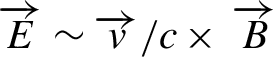 $\overrightarrow{E}\sim \overrightarrow{v}/c\times~\overrightarrow{B}$, and longitudinal. Most importantly, this can be verified with laboratory experiments. So far, we have verified the universality on one of the governing parameters
  ${\omega}_{\mathrm{p}}/{\omega}_{\mathrm{L}}$ though there were only three shots. In the future, by using high-repetition ultra-intense lasers we will address the universality of power-law acceleration on the normalized wave amplitude
  ${a}_0$.
To fully understand the acceleration process of energetic particles or cosmic rays, it is necessary to verify the relation between the observed distribution functions of particles and the waves in the plasma. So far, this has only been possible by in situ observations in space plasmas. For the extragalactic cosmic rays, it is impossible to directly measure the local wakefield, and we had to rely on numerical simulations. The missing link is the wave observations. A coherent wakefield has been observed directly[Reference Matlis, Reed, Bulanov, Chvykov, Kalintchenko, Matsuoka, Rousseau, Yanovsky, Maksimchuk, Kalmykov, Shvets and Downer136]. It is very challenging to observe a turbulent or an incoherent wakefield. We observe the density structures of electrons, such as the filaments in the transverse directions shown in Figures 35 and 39.
Furthermore, as shown in Figure 38, there must be ion acceleration by the wakefield. We will verify this with the current and future ultra-intense lasers. This will complete the verification of the acceleration model by laboratory experiments, that is, we can conclude that the intense precursor waves in the upstream of relativistic collisionless shocks will universally produce power-law spectra with an index of  $-2$. However, this still relies on the numerical results of the precursor excitation via the synchrotron maser instability. We are planning to experimentally verify this with intense lasers. Once we complete this, we can conclude that in the presence of relativistic collisionless shocks, which is reality, there will be universal power-law acceleration of cosmic rays by the wakefield. This will be our long-term goal in this study.
4 Conclusion
This review started with a brief history of the birth of the research field of laboratory astrophysics with intense lasers. It was the dawn of laboratory astrophysics when the supernova SN1987A was observed 33 years ago and the Japanese satellite GINGA clarified that the supernova explodes, while the matter inside is mixed to come to the outer layer by hydrodynamic instability. At the same time, the most critical issue of laser fusion was the physics of turbulent mixing in implosion dynamics owing to the same hydrodynamic instabilities: Rayleigh–Taylor and Richtmyer–Meshkov instabilities.
The similarity of the physics prepared a bridge between astrophysics and laser plasma, although the space–time scale is hugely different. After the proposal of laboratory astrophysics where intense lasers are used in laboratory to model a variety of phenomena to be studied as astrophysics, international collaborations are initiated among theory, computation, laser experiment and astrophysics. Up to the year 2000, many topics had been proposed in several review papers.
In the following two decades, it is awesome to have seen that the physics topics have spread wider, especially to more plasma-oriented topics. They are, for example, collisionless shocks, magnetic field generation, stochastic acceleration of cosmic rays, photoionized plasma, and EOS in giant planets. It is typical that the subjects are basic physics of nonlinear and kinetic plasma physics, and turbulence of the magnetic field and hydrodynamics. In the last two decades, a typical development is the progress of diagnostics with which we could perform challenging experiments. Thanks to such progress, most activities have shifted from theory and computation to real laser experiments.
In the present paper, topics of challenging experiments have been briefly reviewed to introduce much progress to laboratory astrophysics in the last two decades. Two topics out of the 10 have been reviewed in detail in the sections following the brief review. One of the topics is collisionless shock formation via magnetic turbulence mediated by the nonlinearity of Weibel instability in counter-streaming laser-ablation plasmas. The review was given by focusing on the experimental data. Note that this international project was awarded the J. Dawson prize as distinguished research in plasma physics by the APS in 2020.
The other topic is model experiments of cosmic-ray acceleration by turbulent wakefield driven by ultra-short laser pulses. More than a century has passed since the discovery of cosmic rays, whereas there is no direct evidence of the physics of acceleration of particles. In particular, the physics of ultra-relativistic cosmic rays thought to come from outside of our galaxy is still an open question, and any alternative ideas and model experiments are welcome to clarify the physics of relativistic particle acceleration. Note that nonthermal particle acceleration is common phenomena for plasmas in laboratory, space and solar physics, up to cosmology. In addition, the topics also provide laboratory astrophysics research with a new challenge to chaos and stochasticity in modern physics.
Finally, we would like to point out one new challenge for laboratory astrophysics: it is better to say ‘laboratory cosmology’. It has been studied theoretically in the last two decades mainly by Chen et al. [Reference Chen and Tajima137, Reference Chen and Mourou138]. Cosmology has been developed in the frame of general relativity, Einstein equation, with micro physics of elementary particle physics, quantum field theory (QFT) in curved space–time. The QFT has been verified experimentally with the use of accelerators, whereas they are the case only in flat space–time. Cosmology, such as inflation theory, is heavily based on the QFT in the curved space–time[Reference Vilenkin139, Reference Vilenkin140], although there has been no experimental evidence. It is impossible to verify this with accelerators.
Extreme lasers are the only tool to have a possibility to carry out a model experiment to verify QFT in curved space–time[Reference Chen and Mourou138]. We hope an analog of Hawking radiation in blackholes would be a good start to explore this new field[Reference Hawking141, Reference Hawking142]. We hope experimental papers will be published on laser cosmology in the coming two decades.
Appendix: Fusion research and laboratory astrophysics
In the 1990s, laboratory astrophysics became the most attractive subject for me. I found that our knowledge on laser implosion was still immature and we needed further deep study on the physics, especially the hydrodynamic instability and turbulent mixing[Reference Takabe, Yamanaka, Mima, Yamanaka, Azechi, Miyanaga, Nakatsuka, Jitsuno, Norimatsu, Takagi, Nishimura, Nakai, Yabe, Sasaki, Yoshida, Nishihara, Kato, Izawa, Yamanaka and Nakai2]. I was convinced of this conclusion after intensive research to analyze a lot of experimental data obtained by Gekko-XII fusion implosion experiments[Reference Takabe143]. Laboratory astrophysics is an attractive new field for the fusion community and others, because one can approach the core physics of laser fusion by solving many unknown physics in astrophysics. Laser fusion would take a long time, and laboratory astrophysics attracts young peoples to commit to the deepening of the related physics and technologies.
Unexpectedly, I had the opportunity to express such a personal idea in public. The International Congress on Plasma Physics (ICPP ’98) was held in Prague with a gathering of about 1000 scientists. I was asked to give a plenary lecture in this congress. I gave a talk about the status of laser fusion and laboratory astrophysics[Reference Takabe, Nagatomo, Sunahara, Ohnishi, Mahdy, Yoda, Naruo, Azechi, Nishimura and Mima144]. Professor Marshall Rosenbluth (Figure 42) was my next speaker. I was just about to leave the stage when he came up and stood in front of me. He said, ‘Are you going to stay until Friday, the last day of the conference?’ It was Tuesday, and I replied ‘Yes’. Then he said, ‘Well, I organize a panel discussion of “how fusion research should be” on Friday and I ask you to present your comment.’ Later the chairman of ICPP asked me again and he persuaded me that even my personal comment is welcome. Finally, I decided to give my personal opinion for 10 minutes. I gave my talk with the hand-written picture shown in Figure 43.
Professor Marshall Rosenbluth[145].

Until then, I had only presented my research results on laser fusion at international conferences. However, I decided to use this opportunity to express my honest feelings in front of everyone. I made the following declaration in front of fusion researchers around the world while displaying Figure 43.
My research strategy to aim at fusion energy in 1998. This is shown at the stage chaired by Rosenbluth.

‘I will not go down the road to fusion energy only. It seems like a desert road. I want to take a detour to plant and water seeds in flower gardens, and enjoy the sight of beautiful flowers blooming. This may seem like a side trip to you, but to me, it is the shortest way to achieve fusion energy over the long time. That is the path I would like to take from now on.’
After my 10-minute comment, the room was abuzz and many complaints came in, as expected. Some Western researchers said, for example, ‘Who do you think you’re getting paid by to do your research?’ But I rebuffed them by saying, ‘This is my personal opinion and I am not speaking on behalf of my institute.’
I made this declaration with confidence. I already prepared to go my new way and made the declaration in front of the world. On a plane back to home, a professor from UCLA happened to get on the plane beside me and asked me to shake his hand. He said, ‘Your story was excellent.’ I happened to be given the opportunity, and I cannot lie, so I was honest about my feelings, and that is why I spoke up.
After the ICPP’98, the United States decided to withdraw from the ITER program. The paradigm of fusion energy development has shifted dramatically. In other words, the paradigm shifted from a focus on the early realization of fusion energy after the oil crisis to a focus on nuclear fusion as the energy source that would support sustainable development for humanity in the future. For long-term sustainable development, humanity needs energy to prevent global warming. With the end of the Cold War, the perspective of nuclear proliferation had become a very important factor.
The City of Prague and the Vltava river.

Twenty years after Prague (Figure 44), I am convinced that my declaration was correct. As already explained in this paper, laboratory astrophysics has expanded its community around the world and numerous theoretical and experimental studies have been conducted. I believe that laboratory astrophysics has grown to be a research field where young people who wish also to pursue laser fusion can find challenging subjects as a training ground for academic research. Let us take a look in the following at a review of how specifically it has evolved over the past 20 years from what was proposed twenty years ago.
Acknowledgments
We would like to thank T. Minami for his comments. Y. Kuramitsu would like to thank M. Iwamoto for useful discussions. This work was supported by the JSPS KAKENHI under Grant Nos. 19K21865, 19H00668, and 20KK0064.


 Open access