


INTRODUCTION
The Arctic Ocean is very sensitive to changing environmental conditions. Its surface layer is a key component of the Arctic climate system, which serves as the dynamic and thermodynamic link between the atmosphere and the underlying waters (Carmack, Reference Carmack, Lewis, Jones, Lemke, Prowse and Wadhams2000). Thermohaline characteristics of the surface layer are markedly influenced by atmospheric and sea-ice processes, and wind and buoyancy forcing on this important layer ultimately impact the entire upper ocean (Cronin and Sprintall, Reference Cronin, Sprintall, Steele, Thorpe and Turekian2009). The rejection of salt during sea-ice formation strongly impacts upper ocean salinity, so that the stability and development of the ice cover are closely associated with the thermohaline properties of the upper ocean, such as the depth of the mixed layer and halocline. In this context, the Arctic Ocean surface layer is a critical indicator of climate change (Toole and others, Reference Toole2010).
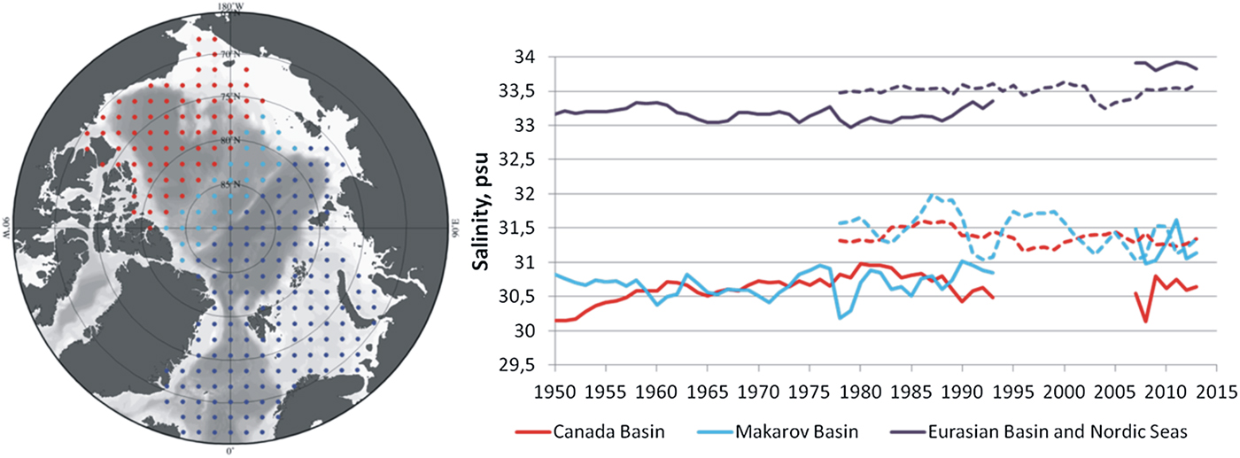
Here, salinity is chosen as the main characteristic of thermohaline structure variations of the Arctic Ocean surface layer because, at high latitudes, it mainly determines the density structure (Weyl, Reference Weyl and Mitchell1968; Morison and Smith, Reference Morison and Smith1981; Walin, Reference Walin1985). The thermohaline structure of the Arctic Ocean surface layer has undergone significant changes in recent years (Macdonald and others, Reference Macdonald, Harner and Fyfe2005). Of particular interest is the great salinification of the surface layer of the Eurasian and Makarov Basins in the early 1990s – a phenomenon unprecedented in the record back to 1950 (Fig. 1). One hypothesis for this is that the increase of Arctic atmospheric cyclone activity in the 1990s led to a large change in the salinity in the Eurasian Basin through changes in river inflow, and increased brine formation due to changes in Arctic sea-ice formation (Dickson, Reference Dickson1999; Polyakov and others, Reference Polyakov2008). The other reason for salinification is the influence of Atlantic waters (AW), which by 2007 became warmer by ~0.24°C than they were in the 1990s. Observations show that increases in Arctic Ocean salinity have accompanied this warming as it was associated with significant shoaling of the upper AW boundary and weakening of the upper ocean stratification in the Eurasian Basin as well. That led to facilitated exchange between AW and the upper layer (Polyakov and others, Reference Polyakov2010). However, recent observations also show that the upper ocean of the Eurasian Basin was appreciably fresher in 2010 than it was in 2007 and 2008 (Timmermans and others, Reference Timmermans2011).
Temporal changes in salinity averaged over the depth range 5–50 m. Dashed curves show salinities from PIOMAS data. Grids with spatial resolution 200 × 200 km were obtained as the result of interpolation and reconstruction (see section ‘Field reconstruction and interpolation’) of bottled and CTD data.
In addition, there have been observations of surface-layer freshening in the Canada Basin. Jackson and others (Reference Jackson, Williams and Carmack2012) emphasized that processes related to warming and freshening the surface layer in this region had transformed the water mass structure of the upper 100 m. With these changes, energy absorbed during summer can enter the deepening winter mixed layer and melt sea ice (Timmermans, Reference Timmermans2015).
The problem of variability of Arctic Ocean salinity is challenging from a theoretical perspective. For example, Lique and others (Reference Lique, Treguier, Scheinert and Penduff2009) performed an analysis of the variability of Arctic fresh water content informed by a global ocean/sea-ice model. The authors uncovered important spatial contrasts in the influence of velocity and salinity fluctuations on ocean fresh water transport variability. They conclude that variations of salinity (controlling part of the Fram fresh water export) arise from the sea-ice formation and melting north of Greenland. Jahn and others (Reference Jahn2012) compared simulations from ten global ocean–sea-ice models of Arctic fresh water, and concluded that improved simulations of salinity variability are required to advance understanding of liquid fresh water export.
Improving the representation of the salinity distribution is crucial. However, inclusion, representation and parametrization of a number of processes is required (Steele and others, Reference Steele2001; Komuro, Reference Komuro2014). For example, in many global ocean–sea-ice models, salt rejection in the first level of the ocean model during ice formation leads to an unrealistic salt distribution in the mixed layer and below (Nguyen and others, Reference Nguyen, Menemenlis and Kwok2009).
The transfer of fresh water and sea ice from the Arctic Ocean to the North Atlantic are significant components of global ocean circulation (Haak and others, Reference Haak, Jungclaus, Mikolajewicz and Latif2003; Gelderloos and others, Reference Gelderloos, Straneo and Katsman2012). Thus, the investigation of the variability of the surface layer (the upper 50 m) can make a significant contribution to understanding ocean-climate feedback. In particular, abrupt changes in surface-layer salinity may lead to critical transitions in the patterns of global ocean circulation, such as convection shut downs and climate disruptions (Hall and Stouffer, Reference Hall and Stouffer2001; Gelderloos and others, Reference Gelderloos, Straneo and Katsman2012). A robust conceptual statistical model may help to describe the features of anomalies in salinification of the Arctic Ocean, which are key players in the formation of surface-layer salinity patterns. In this case, investigation of the structure of patterns and quality of anomalies leads to a better understanding of possible critical transitions in the patterns of global ocean circulation. Variations of Arctic Ocean surface-layer salinity have complex spatial and temporal structures, which are affected by many external factors. Our aim is to distinguish the most significant factors that led to recent changes in surface-layer salinity patterns.
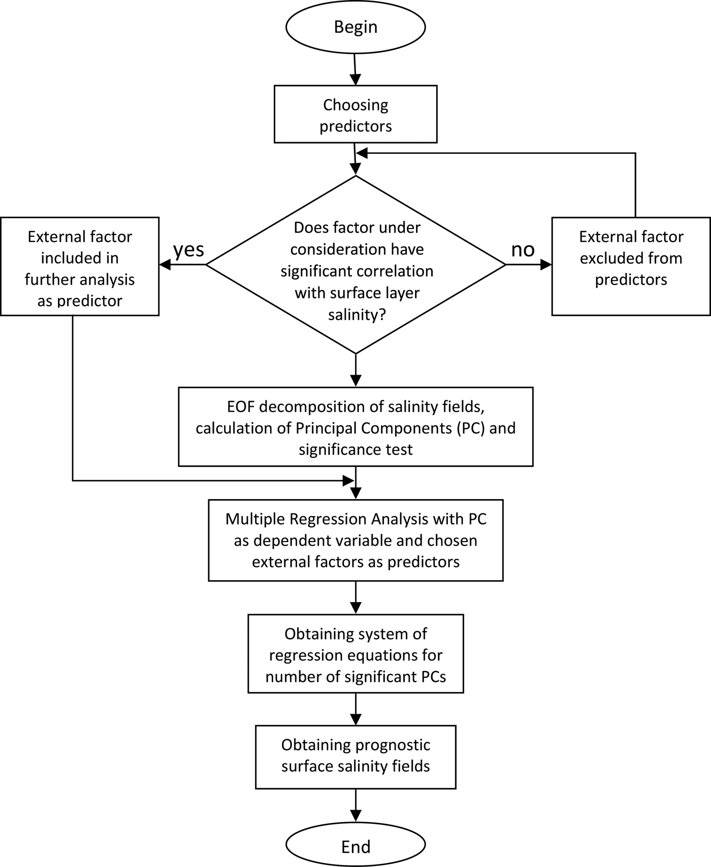
Here, we present a statistical model for Arctic Ocean salinity fields based on multiple linear regression analysis, which builds on ideas presented in prior studies (e.g., Timokhov and others, Reference Timokhov, Chernyavskaya, Nikiforov, Polyakov and Karpy2012). This statistical model of variability of Arctic Ocean winter salinity in the 5–50 m layer is used as a method of reconstruction of observed winter salinity fields presented in Pokrovsky and Timokhov (Reference Pokrovsky and Timokhov2002). The model is based on an empirical orthogonal function (EOF) decomposition of the salinity data (e.g., Hannachi and others, Reference Hannachi, Jolliffe and Stephenson2007), and a multiple correlation analysis of the time series associated with the first three leading modes, or principal components (PCs); see Appendix Box 1 for a schematic diagram of the model. The contribution of atmospheric factors and hydrological processes in the spatial distribution of surface-layer salinity was interpreted by determining the structure of the multiple correlation equations. The variability patterns and relationships identified through the statistical analysis and modeling inform a conceptual model for principal drivers of Arctic salinity.
METHODS
Data set
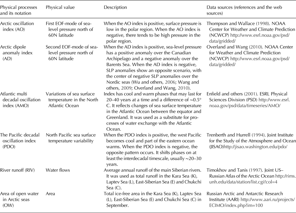
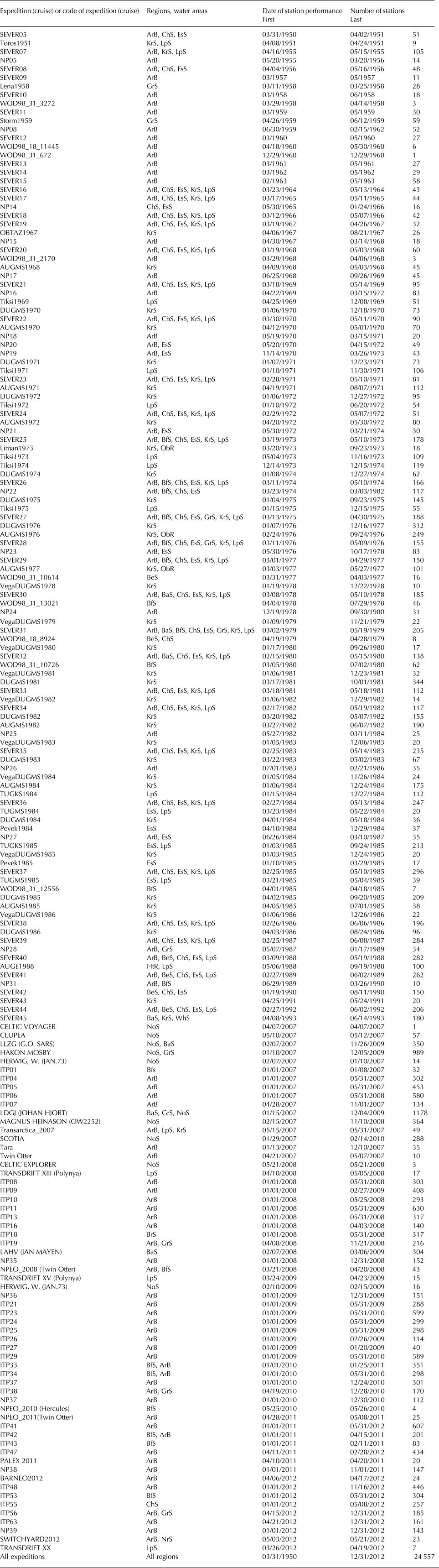
This study is based on a collection of more than 9800 instantaneous temperature and salinity profiles, with data available at the standard levels (5, 10, 25, 50, 75, 100, 150, 200, 250, 300, 400, 500, 750, 1000 and so on every 500 m), collected between 1950 and 1993. The data were obtained from the Russian Arctic and Antarctic Research Institute (AARI) database, which was also used in the creation of the Joint US–Russian Atlas of the Arctic Ocean for winter (Timokhov and Tanis, Reference Timokhov and Tanis1997). The AARI database was first introduced by Lebedev and others (Reference Lebedev, Karpy, Pokrovsky, Sokolov and Timokhov2008). This is complemented by the data made available over the period 2007–2012 from the expeditions of the International Polar Year (IPY) and afterward, which consist of Conductivity Temperature Depth (CTD) and eXpendable Conductivity Temperature Depth (XCTD) data, as well as data from the Ice-Tethered Profiler (ITP)-buoys (more than 14 600 stations in total). The average vertical resolution of all these profiles was 1 m. In areas where observations were missing, temperature and salinity data were reconstructed in a regular grid for the period 1950–1989 as detailed in the next subsection. The time period of 1994–2006 was not included in the analysis as there are too few data to construct reliable gridding fields. Thus, the working database is represented by grids with 200 km horizontal spacing, covering the deep part of the Arctic Ocean (with depths of more than 50 m). According to Treshnikov (Reference Treshnikov1959), Rudels and others (Reference Rudels, Anderson and Jones1996, Reference Rudels, Jones, Schauer and Eriksson2004) and Korhonen and others (Reference Korhonen, Rudels, Marnela, Wisotzki and Zhao2013), the average thickness of the Arctic Ocean mixed layer for the winter season is ~50 m. A description of the data sources for other physical parameters, used as predictors for the statistical model, can be found in Table 1.
Predictors used for the approximation of PCs
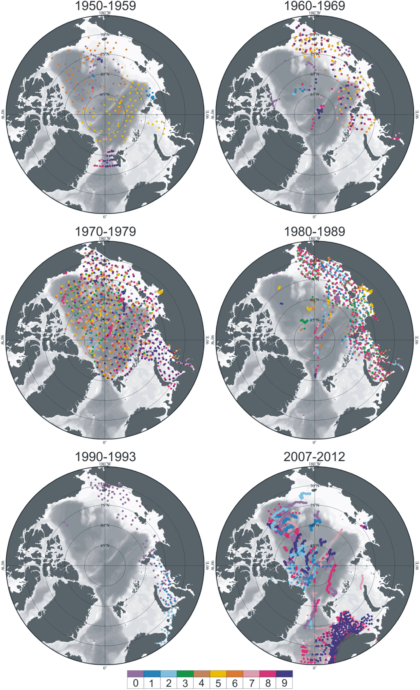
The database used in this study belongs to the Oceanography Department of the Arctic and Antarctic Research Institute and it is not freely available. To mitigate the related issues, we provide additional data description. Table A1 in the Appendix contains a list of the expeditions and number of stations that were used for reconstruction and gridding of salinity fields. Figure A1 shows the overall observation density and the year associated with each observation. The data exhibit a spatiotemporal non-uniformity that is undesirable but expected given the logistical challenges associated with recovering long-term observations of Arctic salinity. While this dataset has gaps and is proprietary, we believe it provides one of the most spatiotemporally detailed observational resources for studying multidecadal variations in basin-wide Arctic salinity. This manuscript is motivated by the potential to advance understanding through identification, dissemination and modeling of the principal modes of variability in these long-term salinity observations.
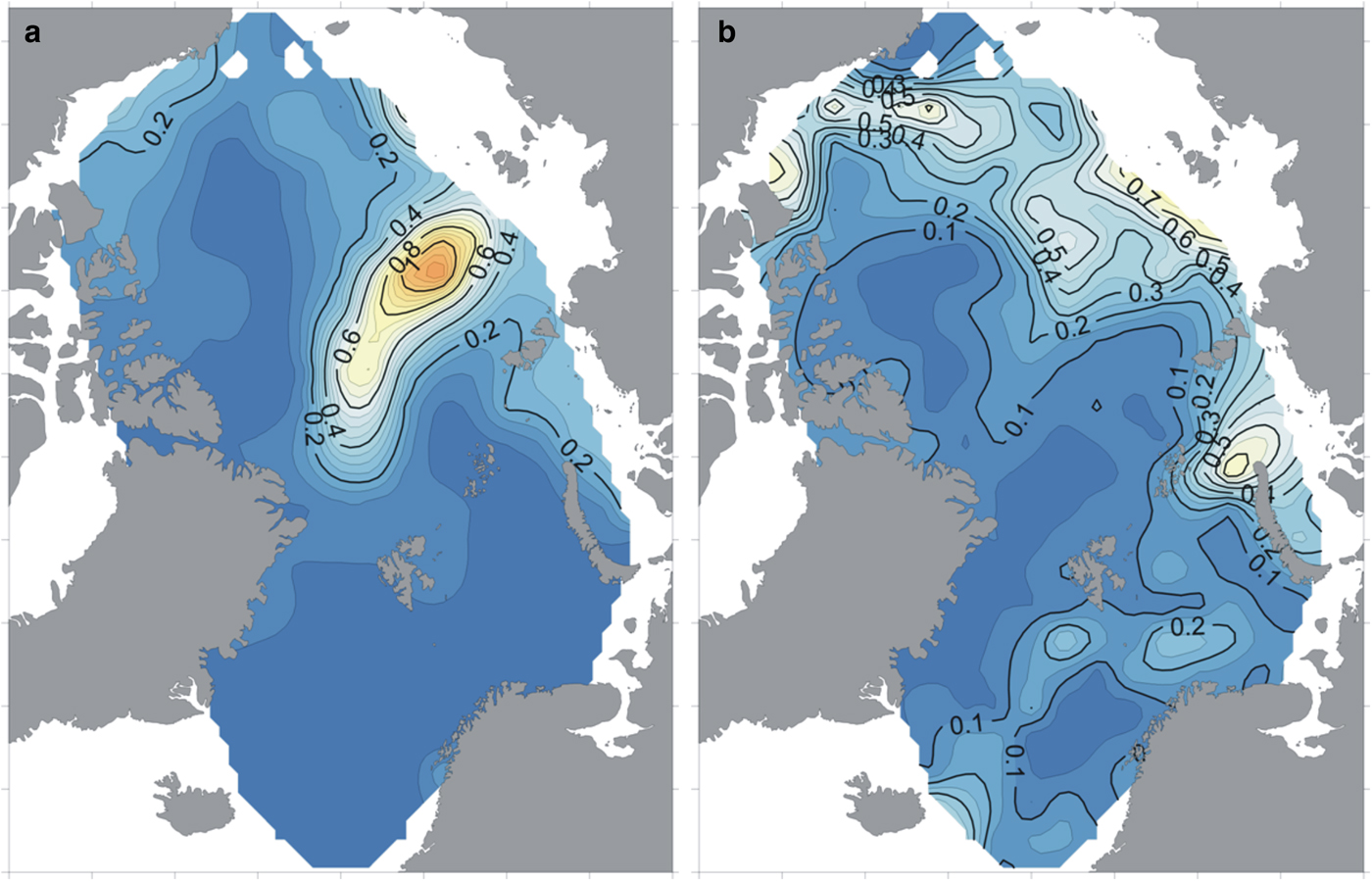
Gridded fields of surface winter salinity were compared with fields from the Pan-Arctic Ice-Ocean Modeling and Assimilation System (PIOMAS; Zhang and Rothrock, Reference Zhang and Rothrock2003; Lindsay and Zhang, Reference Lindsay and Zhang2006) for their overlapping period 1978–1993 (dashed curves, Fig. 1). PIOMAS is a coupled ice-ocean model which uses data assimilation methods for ice concentration and ice velocity. Forced by atmospheric observations, its output is available for 1978 to near present and is widely used as a reference for Arctic variables with limited long-term observations including salinity and sea-ice thickness. Maps of long-term means for both datasets are similar (Figs 2a and A2a), with a correlation coefficient of 0.88. Nevertheless, PIOMAS data generally provide higher salinity values for the Amerasian Basin (Canada Basin together with Makarov Basin) for the overlapping period (Fig. 1). The associated variance maps are also significantly correlated with each other (correlation coefficient R = 0.36; statistical significance level p = 0.05) but exhibit some salient differences (Fig. A3). In particular, a high variance zone along the Lomonosov Ridge is prominent in the AARI dataset, but is absent in PIOMAS data. PIOMAS instead features several centers of high variance along the shelf.
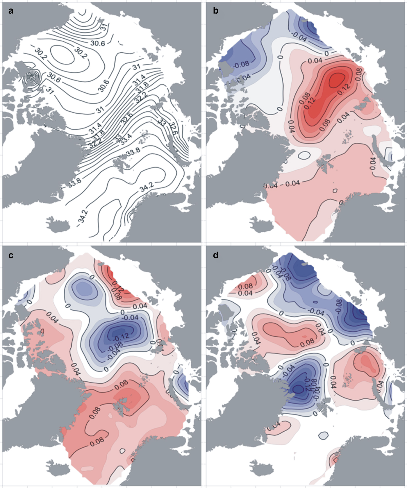
The average salinity field (a) and first three modes of the average salinity field decomposition for the layer 5–50 m: (b), (c), (d) – first, second and third modes, respectively, for the periods 1950–1993 and 2007–2012.
To test for artifacts from the data gaps and the interpolation procedure (reviewed in the next subsection), we make several comparisons across methods and to independent datasets in the subsections to follow. For example, we also performed the EOF analysis with and without the additional 2007–2012 period, and report only modest change to the resulting modes of variability (section ‘Decomposition of surface-layer salinity fields by EOF’). In section ‘Decomposition of surface-layer salinity fields by EOF’, we also compare EOFs from the AARI data to those from PIOMAS.
Field reconstruction and interpolation
To provide temporal and spatial continuity, we have unified existing datasets using reconstruction and gridding. The technique of computing gridded fields for the period from 1950 to 1993 was described by Lebedev and others (Reference Lebedev, Karpy, Pokrovsky, Sokolov and Timokhov2008), and is summarized here.
These techniques are based on the method of ocean field reconstruction, proposed by Pokrovsky and Timokhov (Reference Pokrovsky and Timokhov2002). This method, which was used to obtain gridded salinity fields, is given by
 $$\eqalign{z_i = & z_i^{\left( r \right)} + e_i,\; \; {\langle} z_iz_j{\rangle} = \sigma _{x_ix_j},\; \; {\langle}z_ie_i{\rangle} = 0, \cr {\langle}e_i{\rangle} = & 0,\; \; {\langle}e_ie_j{\rangle} = \delta _{ij}\sigma _{\rm e}^2 = \sigma _{{\rm e}_{ij}}^2.} $$
Here z(t, x) is the measured value of an oceanographic variable (e.g., temperature or salinity), and is a random function of time t and spatial coordinates x; i and j are the nodes of the irregular data grid; the notation <…> denotes the ensemble average of a value. We can write the observed value of z(t, x) as the sum of a true value z (r)(t, x) of the oceanographic variable and an observational error e(t, x). In addition, we introduce  $\sigma _{x_ix_j}$ as a std dev. of spatial coordinates and $\sigma _{{\rm e}_{ij}}^2 $ as a std dev. of errors. We also propose that z i(r) has spatial correlations to the oceanographic parameters; that a systematic error is not identified; a std dev. of error (σ e2) does exist; and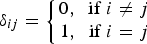 $\delta _{ij} = \left\{ {\matrix{ {0,\; \; {\rm if}\; i \ne j} \cr {1,\; \; {\rm if}\; i = j} \cr}} \right.$ is the Kronecker δ.
Biorthogonal decomposition of the oceanographic variable can help to identify the connections between spatial and temporal distributions within the data:
 $$z\left( {t_j,\; x_i} \right) = \mathop \sum \limits_k c_k^j f_k\left( {x_i} \right) + e(t_j,x_i),$$
where f k(x i) is the spatial EOF, and c kj is the calculated coefficient or so-called k th PC.
As the next step, we approximate the EOF through linear combinations (with coefficients b kl) of convenient analytical functions P l(x i) (e.g., polynomials, splines, etc.):
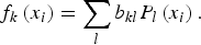 $$f_k\left( {x_i} \right) = \mathop \sum \limits_l b_{kl}P_l\left( {x_i} \right).$$
Thus, the modified biorthogonal decomposition can be written as
 $$z\left( {t_j,\; x_i} \right) = \mathop \sum \limits_k d_l^j P_l\left( {x_i} \right) + e(t_j,\; x_i),$$
where  $d_{l}^{j} = \mathop \sum {b}_{kl}\;c_k^j $.
The main goal of this spectral analysis method is to estimate the coefficients of spectral decomposition  $\{ c_k^j \} $ and {b kl}, in order to identify dominant modes of behavior. In this case, we rewrite formula (2) in the following matrix form:
 $$Z = F \, \cdot \, C + e,$$
where · denotes matrix multiplication.
The matrix F is formed by the values of the EOF, the matrix Z is composed of the totality of the measurement data at the points of the observation net x i, and the matrix e is filled out by observational error values.
The system of linear equations (5) with respect to the unknown coefficients  $c_k^j$ can be solved on the basis of the a priori statistical information (1) with the use of the standard estimation of the least squares method. A formula for the estimation of the matrix of the unknown coefficients C was obtained in (Pokrovsky and Timokhov, Reference Pokrovsky and Timokhov2002), and is written
 $$\hat C = (F^{\rm T} \, \cdot \, K_{\rm e}^{ - 1} \, \cdot \, F + K_{\rm c}^{ - 1} )^{ - 1}F^{\rm T} \, \cdot \, K_{\rm e}^{ - 1} \, \cdot \, Z^{\prime},$$
where X −1 and XT denote the inverse and transpose of a matrix X, respectively. The covariance matrix of errors of the expansion coefficients K c is a diagonal matrix composed of eigenvalues of the covariance matrix K z. Here, the matrices K z and K e are covariance matrices of the std dev. of spatial coordinates and the std dev. of errors, respectively.
In order to obtain an estimate of the unknown variables at the nodes of the regular grid  $\tilde x_i$, it is necessary to interpolate the EOF into the corresponding nodes of the grid and obtain a new matrix $\tilde F$ of the EOF, a new matrix $\tilde C$ of decomposition coefficients, and new matrix $\tilde e$ of observational errors. Using the matrix $\tilde F$ obtained in this way and the estimates of the coefficients $\hat C$ from formula (6), from the matrix relationship
 $$\tilde Z = \tilde F \, \cdot \, \tilde C + \tilde e,$$
we obtain an estimate of the unknown parameters at the nodes of a regular grid. Simultaneously with the salinity fields in the nodes of a regular grid, we can also calculate the covariance matrices of the errors of estimations obtained from the following equations:
 $$K_{\hat{\rm C}} = \left( {I + \left( {K_{\rm c} \, \cdot \, \left( {{\tilde F}^{\rm T} \, \cdot \, \tilde K_{\rm e}^{ - 1} \, \cdot \, \tilde F} \right)} \right)} \right)^{ - 1} \, \cdot \, K_{\rm c},$$
 $$K_{\hat{\rm Z}} = \tilde F \, \cdot \, K_{\rm z} \, \cdot \, \tilde F^{\rm T},$$
where I is the identity matrix and  $\tilde K_{\rm e}^{ - 1} $ is the covariance matrix of the observation error expanded over the regular grid x i.
This approach is a combination of singular value decomposition and statistical regularization. These coefficients (modes) can be linked to the real physical processes that influence salinity as presented in section ‘Statistical approach’. Preparation of the average salinity field data for 2007–2012 consisted of several stages as detailed in the Appendix. First, we checked the data for random errors. Then, we used linear interpolation and assimilated the real plane with the field data through the virtual plane of data. Next, we constructed an interpolation via a grid of nodes (separately for each plane). The gaps in the data for uncovered sites were filled with climatic values from the Joint US–Russian Atlas of the Arctic Ocean (Timokhov and Tanis, Reference Timokhov and Tanis1997). Using an older climatology to fill in recent (2007–2012) salinity fields is appropriate here as the areas where the most significant changes are observed, i.e., Canadian and Eurasian Basins, have sufficient data coverage to lessen concerns about potential inaccuracies (Fig. A1).
Statistical approach
Here we describe the approaches to data analysis which were used for physical interpretation of our statistical model. Polyakov and others (Reference Polyakov2010), Rabe and others (Reference Rabe2011) and Morison and others (Reference Morison2012) have emphasized that the thermohaline structure of the surface layer has undergone significant change over the last decade. However, there is still room for discussion on what physical processes led to these changes or what the future trends may be.
The analysis of the variability of the surface layer (including salinity fields) of the Arctic Ocean may be based on a decomposition using EOFs. This approach is useful in our case because decomposition by EOF analysis gives modes (spatial patterns) and PC time series, which allow us to divide the variability into spatial and temporal components. Each mode describes a certain fraction of the total variance of the initial data, and the EOFs are conventionally ordered so that the first EOF explains the most variance and subsequent EOFs explain progressively less variance (Hannachi and others, Reference Hannachi, Jolliffe and Stephenson2007). The first three modes describe more than half the variance of the analyzed fields as further detailed below, which allows significant compressing of the information contained in the original data (Hannachi and others, Reference Hannachi, Jolliffe and Stephenson2007; Borzelli and Ligi, Reference Borzelli and Ligi1998). The EOF decomposition was carried out for the average salinity fields for the layer 5–50 m, yielding PCs for the periods of 1950–1993 and 2007–2012.
Multiple linear regression was used to model the PC time series to identify predictors that determined variability of the salinity fields. The regression equations can give projections of future changes because the predictors lead the salinity field by various temporal lags. The statistical model is characterized by a system of linear regression equations constructed for the first three PCs. The candidate predictors were as follows: atmospheric circulation indices (Arctic oscillation (AO) and Arctic dipole (AD) indices; see Table 1) calculated for winter (October–March to cover the period of active ice formation) and summer (July–September to cover the period of active ice melting), river runoff, the area of the ice-free surface in Arctic seas in September and water exchange with the Pacific and Atlantic Oceans. For the latter two water exchanges, we used the Pacific decadal oscillation (PDO) and Atlantic multidecadal oscillation (AMO) indices as respective proxies because of their influence on the temperature and salinity of water, which is entering through the Bering Strait and the Faeroe-Shetland Strait to the Arctic Ocean (Zhang and others, Reference Zhang, Woodgate and Moritz2010; Dima and Lohmann, Reference Dima and Lohmann2007). Atmospheric indices were averaged by different time periods within indicated winter and summer seasons. The optimal periods of averaging for a particular index were chosen on the basis of maximal correlations with PCs.
RESULTS
Decomposition of surface-layer salinity fields by EOF
As a result of EOF decomposition of the salinity fields for the 5–50 m layer, we obtained two sets of modes and PCs – one for the period of 1950–1993 (series 1) and one for the same period adding the years 2007–2012 (series 2). North's rule of thumb states the following: if the sampling error in an eigenvalue is comparable to the distance to a neighboring eigenvalue, then the sampling error of the EOF will be comparable to the size of the neighboring EOF (North and others, Reference North, Bell, Cahalan and Moeng1982). Based on this rule, the first three modes were accepted for further analysis as physically significant. The first three modes obtained by the decomposition of series 1 describe more than 55% of the total dispersion of the initial fields. The first three modes of series 2 describe more than 61% of the total dispersion. Nevertheless, the first modes for both decompositions have very similar shapes. The only differences are a more distinct dipole structure between the Canada Basin and Eurasian Basin, and positive EOF loading (instead of negative in the first mode of series 2) over much of the Nordic seas that appears in the first mode of series 2. As the Nordic seas region is the pathway of AW in the Arctic Basin (Karcher and others, Reference Karcher, Kauker, Gerdes, Hunke and Zhang2007), we assume that the change of sign of EOF values is associated with increased temperature and salinity of AW inflow and subsequent salinification of the Eurasian Basin (Polyakov and others, Reference Polyakov2010; Beszczynska-Möller and others, Reference Beszczynska-Möller, Fahrbach, Schauer and Hansen2012). Thus, the modes obtained by decomposition in series 1 cannot take into account the essential features of the distribution of surface-layer salinity fields associated with the salinification of the Eurasian Basin. Therefore, for further analysis we used the PCs and modes obtained upon decomposition in series 2 (Fig. 2).
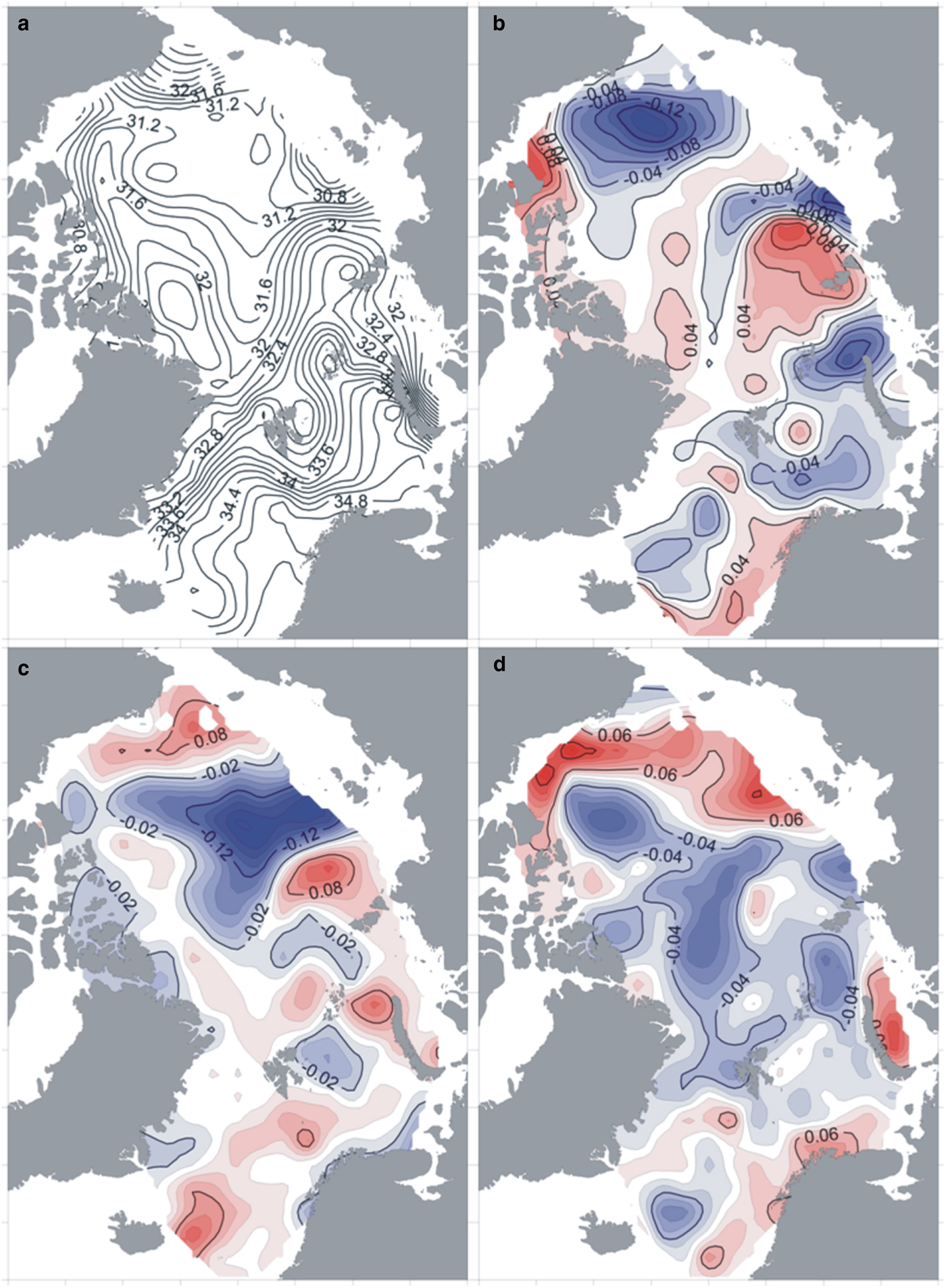
As a point of comparison for these EOFs, Appendix Fig. A2 presents a similar EOF analysis using model output from the PIOMAS. The spatial pattern of PIOMAS mean salinity (Fig. A2a) reasonably resembles the pattern shown for our data in Figure 2a. EOFs of PIOMAS salinity after detrending (Figs A2b–d) repeat the main features of corresponding results in Figure 2b–d, despite incomplete overlap over the analysis periods. In particular, for both datasets, the leading EOF for salinity features a prominent dipole between the Canada Basin and Eurasian Basin (Figs 2b and A2b). However, the leading EOF of PIOMAS salinity has a more patchy structure. In particular, there are negative centers of action situated along the Siberian shelf break, along with freshened areas (Fig. A2a) that are not as clearly pronounced in the AARI salinity data (Fig. 2a). The second EOF of salinity features a negative center of action elongated along the Lomonosov Ridge surrounded by positive loading strongest along Siberian shelf (Figs 2c and A2c). Less agreement is seen for the third EOF (Figs 2d and A2d), which is perhaps unsurprising in moving toward modes accounting for less variance.
The linear regression equation for the PCs
We present here a statistical model of interannual variability of Arctic Ocean surface-layer salinity. This research builds on already established approaches used by Pokrovsky and Timokhov (Reference Pokrovsky and Timokhov2002), specifically their reconstruction of salinity fields applying modified EOF methods.
We suggest some additions to improve on the ideas presented in previous research by Timokhov and others (Reference Timokhov, Chernyavskaya, Nikiforov, Polyakov and Karpy2012). For example, the analysis presented is based on a dataset updated for the period 2007–2012, which is important for understanding the physical processes during the dramatic recent changes in Arctic sea ice. The area under consideration was extended and includes the Nordic seas and part of the Siberian shelf with depths of more than 50 m. This expanded domain allowed consideration of the areas strongly influenced by river runoff and ice processes, and makes visible their effects on the structure of the EOFs. Also, in contrast to our previously published research (Timokhov and others, Reference Timokhov, Chernyavskaya, Nikiforov, Polyakov and Karpy2012), we do not use the previous values of the PCs (history) as predictors for linear regression, which simplifies the physical interpretation of the equations obtained.
A set of external factors having the most correlation with salinity values (the predictors as described in section ‘Statistical approach’) have been defined based on the results of correlation analysis. As a result of linear regression analysis, we obtained empirical equations for the first three PCs (see Table A2 in Appendix). The structure of these equations can be explained through the sets of factors that simulate the effects of both atmospheric and hydrological processes.
Thus, the predictors used can be divided into two groups. The first group includes atmospheric circulation indices and reflects the influence of atmospheric processes. The second group corresponds to hydrological processes: river runoff into Arctic seas, inflows through the Bering Strait and the Faeroe-Shetland Strait, which were characterized by the PDO and AMO indices, and the areas of open water in the Arctic seas in September. Predictors were included in the equations with different time shifts (lags). The value of the time shift was 1–10 years and was chosen to maximize correlations of predictors with the PCs as noted above.
The contribution of each group to the explained variance in PC1 through PC3 can be calculated based on the magnitude and sign of the regression coefficients of corresponding predictors included in that particular group. In this case, hydrological processes have a dominant contribution to the explained variance of all PCs (from 86 to 61%). Atmospheric factors (i.e., AO and AD) contribute from 14 to 39%.
DISCUSSION AND SUMMARY
The first mode of the surface-layer salinity decomposition (EOF1) displays an out-of-phase relationship between salinity anomalies in the Canada and Eurasian Basins (which includes the Nansen and Amundsen Basins) and Makarov Basin (Fig. 2b).
In the late 1980s, as a consequence of surface air temperature rising, the atmospheric circulation regime in the Arctic began to change (Steele and Boyd, Reference Steele and Boyd1998; Proshutinsky and others, Reference Proshutinsky2009; Morison and others, Reference Morison2012). Degradation of the Arctic anticyclone, shifting of the pressure pattern in the Beaufort Sea counterclockwise from the 1979–1992 pattern (Morison and others, Reference Morison, Aagaard and Steele2000) and strengthening of the dipole pressure pattern (Overland and others, Reference Overland and Wang2010) were observed. According to Wang and others (Reference Wang2009), large values of the AD indices (higher than 0.6 std dev.) could be a primary reason for the historical record lows of sea-ice extent in the summers of 1995, 1999, 2002, 2005 and 2007. In addition, in the late 1980s, the inflow of warm and highly saline AW into the Arctic Basin increased (Morison and others, Reference Morison, Aagaard and Steele2000; Polyakov and others, Reference Polyakov2010). Observed shoaling of the AW upper boundary, together with a decrease of static stability in the halocline layer, led to an increase in upper layer temperature and salinity in the Eurasian Basin (Polyakov and others, Reference Polyakov2010). At the beginning of this century, the heat flux through the Bering Strait to the Chukchi Sea increased (Woodgate and others, Reference Woodgate, Weingartner and Lindsay2010). Comparatively warm and fresh (salinity range 31< S < 32) summer Pacific waters, due to their low density, were able to inject heat close to the ocean surface (Stigebrandt, Reference Stigebrandt1984) and enhance ice melting in the Canada Basin (Shimada and others, Reference Shimada2006) which led to decreasing surface-layer salinity in this region.
These observations allow us to suggest that salinity differences between the Canada Basin and Eurasian Basin, which became more pronounced in recent years (Fig. 1), are the consequence of these processes. Our suggestion is supported by the regression equation for PC1 (Table A2) from which we see that PC1 is a function of AMO, PDO, open water area in the East Siberian and Chukchi seas (that can be considered as an indirect indicator of fresh water inflow from these seas to the Arctic) and summer AO index. The time lags must be related with the time that it takes for Atlantic and Pacific waters to reach the Arctic Basins and become involved in associated circulation.
According to Karcher and others (Reference Karcher and Oberhuber2002), travel time for the propagation of anomalies in AW is 5–10 years from the Nordic Seas to the Eurasian Basin. This is reflected by AMO time lags. Bourgain and Gascard (Reference Bourgain and Gascard2012) revealed that the warm signal from the Bering Strait propagated in the interior of the Canada Basin over 4–5 years. A proxy of this process is the PDO. The travel times for the Siberian river water from the river mouths to the shelf edge are estimated to be 2–5 years (Schlosser and others, Reference Schlosser, Bauch, Fairbanks and Bönisch1994; Karcher and others, Reference Karcher and Oberhuber2002). These time periods are in good agreement with time lags of the statistical model predictors, which may vary from 3 to 10 years (Table A2).
EOF2 exhibits opposite polarity of salinity anomalies in the central Arctic Ocean and near-slope areas (Fig. 2c). Spectral analysis of the associated PC2 revealed a 9-year cycle (periodogram is not shown here), which we associate with shifts between cyclonic and anticyclonic circulation regimes (Proshutinsky and Johnson, Reference Proshutinsky and Johnson1997; Rigor and others, Reference Rigor, Wallace and Colony2002). The regression equation for PC2 demonstrates its dependence on the summer AO and AD indices. Thus, during an anticyclonic regime of atmospheric circulation, fresh surface waters tend to flow to the center of the Arctic basin and negative salinity anomalies form there. At the same time, along the slopes there is upwelling of AW and positive salinity anomalies occur (Proshutinsky and Johnson, Reference Proshutinsky and Johnson1997). During a cyclonic circulation regime, reversed momentum forcing should likewise produce positive salinity anomalies in the central Arctic and negative salinity anomalies along the slopes.
The contribution of each predictor in the variability of a particular PC was evaluated as:
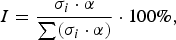 $$I = \displaystyle{{\sigma _{i} \cdot \alpha} \over {\mathop \sum \nolimits (\sigma _i \cdot \alpha )}} \cdot 100\%, $$
where σ i is the std dev. of the predictor and α is the regression coefficient of the predictor. According to this formula, contributions of the predictors for PC2 (Table A2) were calculated. PDO and river runoff from the Laptev, East Siberian and Chukchi Seas make the largest contribution to the variability of PC2 (33.8 and 26.9%, respectively) with slightly weaker effects from AO and AD (20.5 and 18.9%).
EOF3 is represented by a field with multicore structure (Fig. 2d). The positive centers of action spread from the Beaufort Sea over the North Pole to the Kara Sea and are surrounded by negative centers of action. This kind of distribution is associated with an AD (Wu and others, Reference Wu, Wang and Walsh2006). The winter AD index accounts for ~22% of the variability of PC3. The most distinct negative cores are located along the shelf of the Laptev and Chukchi Seas and also near Greenland. In our statistical model, associated variations are accounted for by river runoff from the Laptev, East Siberian and Chukchi Seas, the PDO index, and the AMO index, which account for 20, 25.8 and 32.4% of the variability of PC3, respectively (Table A2).
All predictors included in the regression equations (with particular time lags and averaging periods) are statistically independent, i.e., they are not significantly correlated with each other, except for AMO (−10) and PDO (−3). These indices have a slight positive correlation (R = 0.33), but this is not a concern because they have different regions of influence and are associated with different proxies.
Time series of PC1−3 show a mixture of interannual and quasidecadal oscillations (Fig. 3). Based on the configurations of the EOFs (Fig. 2), the regression equations (Table A2) and results of the spectral analysis of the PCs, we may assume that large-scale surface-layer salinity anomalies (with periods longer than 20 years) are the result of water exchange effects. The shorter period (8–9 years) variations appear to be determined by atmospheric circulation processes. Also, interannual variations occur due to interannual variability of both atmospheric and hydrological processes.
The actual (black line) principal components and calculated principal components (red dashed line) with the help of the equations of linear regression. Correlation coefficients between the calculated time series of PCs and actual PCs are: r(PC1) = 0.88; r(PC2) = 0.73; r(PC3) = 0.55.
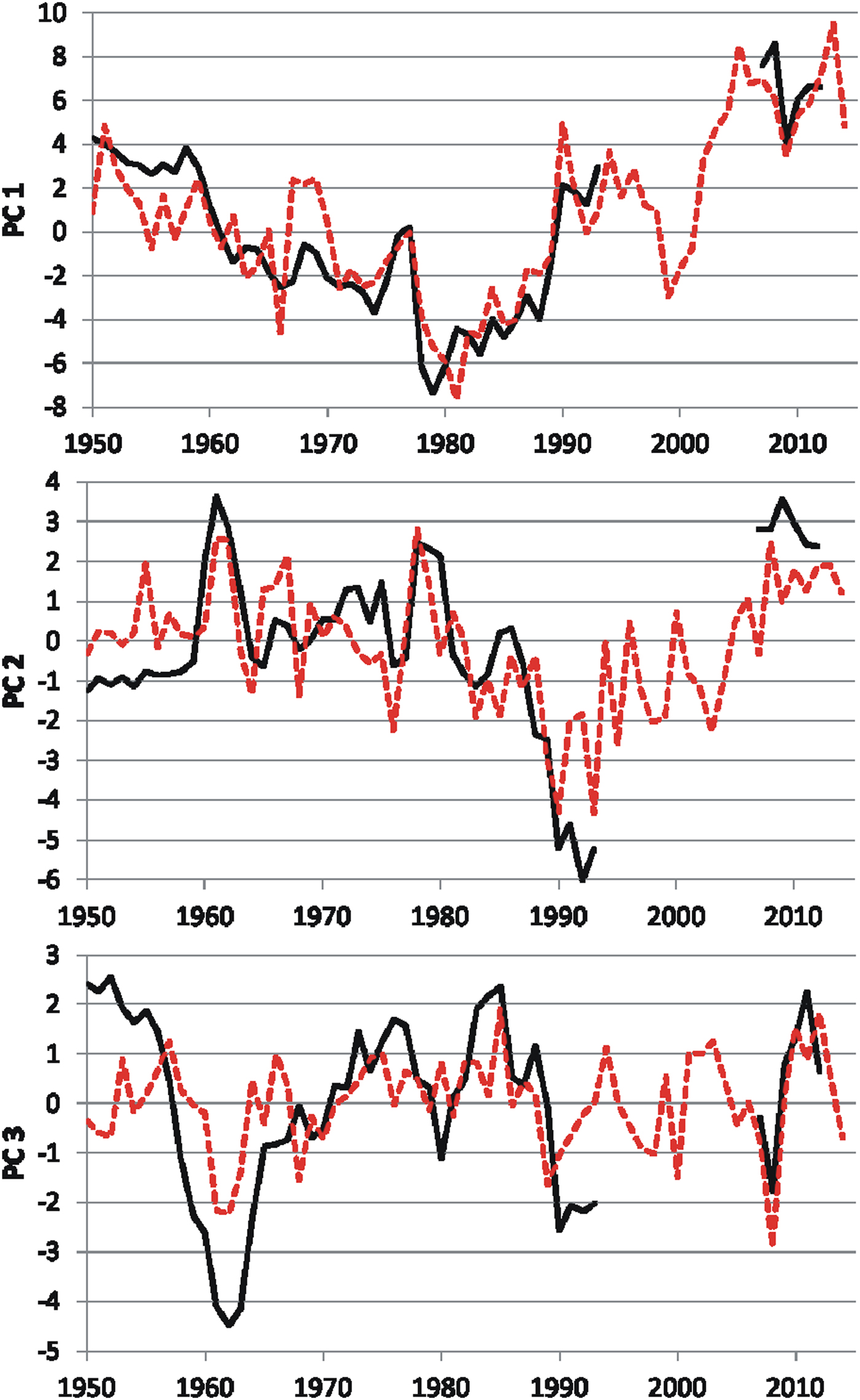
The derived equations in the Appendix (Table A2) describe the first three PCs for the period 1950–2012. Calculated with these equations, the modeled PCs agree well with the values of the PCs directly derived from the decomposition of salinity fields via EOF analysis (Fig. 3).
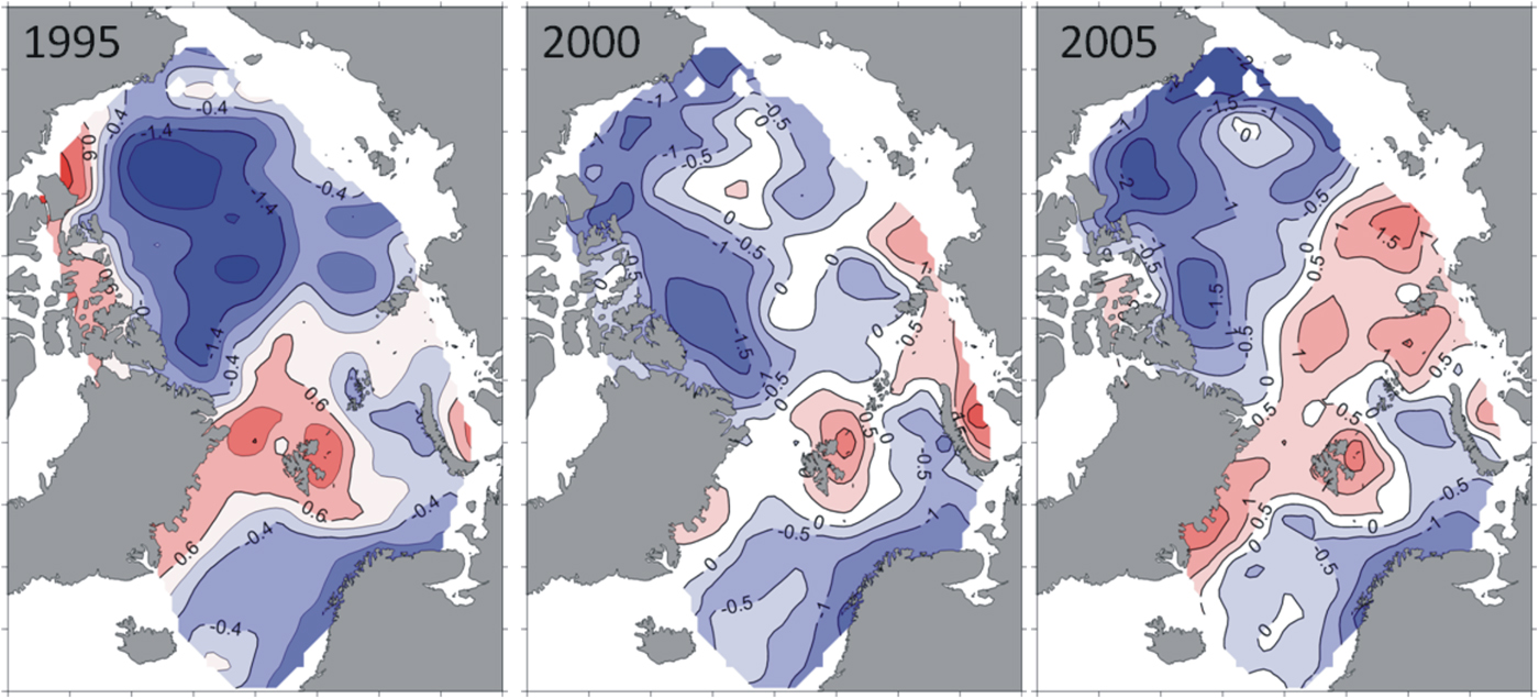
Theoretically, the salinity fields for 1994–2006 can be reconstructed using this statistical model. We noted above that this period had gaps in observational data. The salinity fields of 1995, 2000 and 2005 were chosen for reconstruction to demonstrate the capabilities of the statistical model. The results were compared with PIOMAS model data. Although reconstructed fields have high significant correlations with the PIOMAS fields (correlation coefficients are 0.84, 0.88 and 0.81), in the Amerasian Basin they show lower salinity values than the PIOMAS data. Differences in this region may reach 2 psu. In the Eurasian Basin, specially over the Lomonosov Ridge, the reconstructed salinity values are higher than the PIOMAS data with differences of up to 1.5 psu (for 2005) (Fig. 4).
Maps of differences of salinity fields reconstructed with the statistical model and those from PIOMAS data.
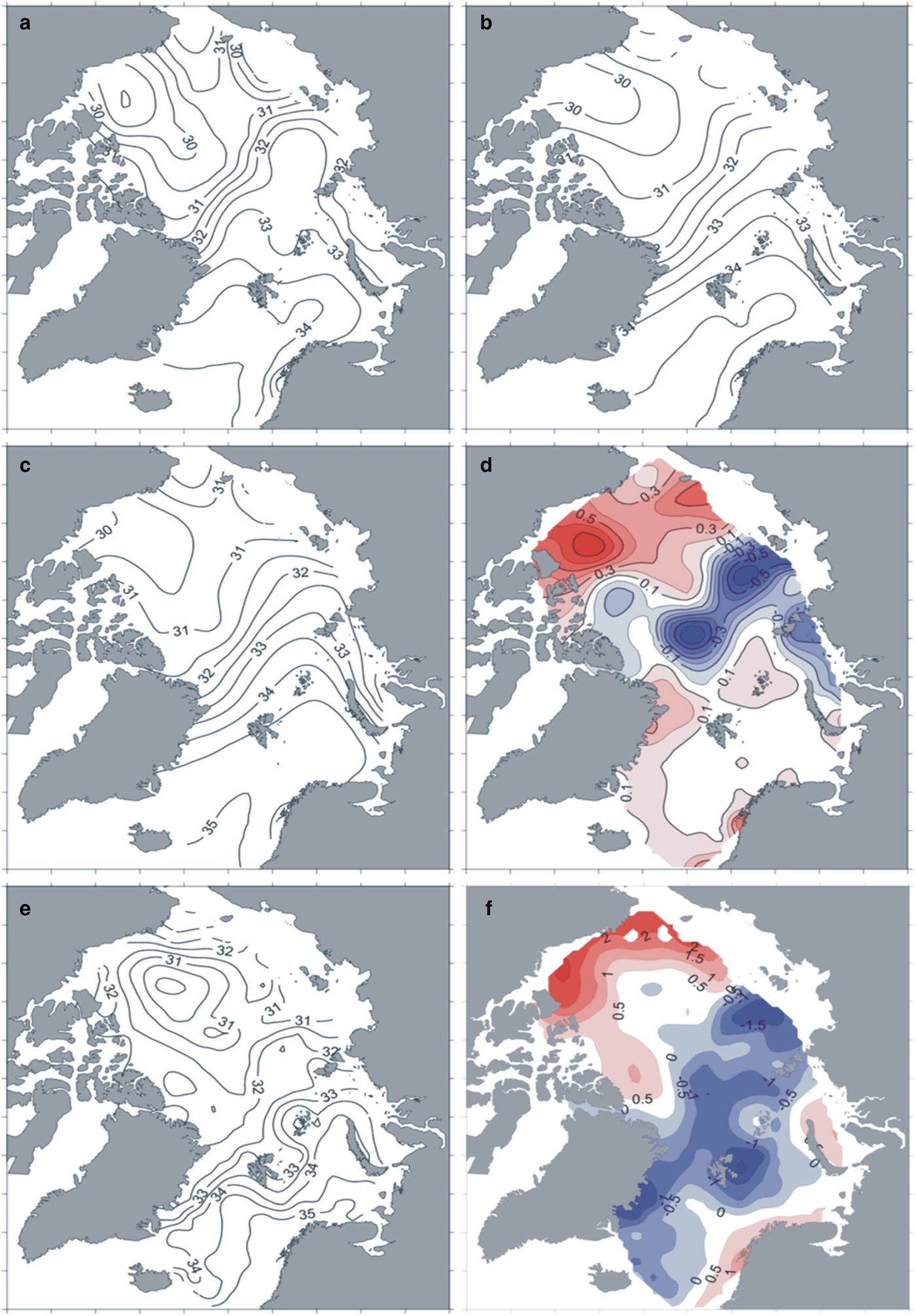
We also applied our statistical model to the reconstruction of salinity fields for 2013–2014, extending beyond the data record in order to develop a retrospective forecast (sometimes referred to as a hindcast). As a result, we obtained salinity fields that correspond to the trends observed in recent years. This preserved the freshening in the Canada Basin as well as salinification of the surface layer over the Lomonosov Ridge (compared with average surface-layer salinity for 1961–1990) (Fig. 5). According to our modeled values for 2013–2014, freshened water from the Beaufort Gyre should have moved westward along the Canadian Continental Slope in 2013. There are also negative salinity anomalies observed in the Arctic seas along the Siberian shelf. These processes were able to freshen the Eurasian Basin slightly so that in 2014 positive salinity anomalies over the Lomonosov Ridge were lower than in 2013. To demonstrate the quality of the forecast, we compared the salinity field for 2013 with the corresponding gridded field of observational data and PIOMAS data (Fig. 5). As we were not able to find enough data in winter 2014 to produce a reliable gridded field, comparison for this year was not conducted. In both cases, the reconstructed values are lower in the Canadian Basin and higher in the Eurasian Basin. However, our results are closer to the observational data than to the PIOMAS data, as differences in the first case are not larger than 0.7 psu (Fig. 5d), and in the second case, they are as large as 2.5 psu (Fig. 5f). In any case, PIOMAS data always show higher salinity values in the Amerasian Basin and lower values in the Eurasian Basin than prognostic or reconstructed fields. Some discrepancies from PIOMAS are expected for at least two reasons. First, PIOMAS salinity fields are simulated values not directly guided by salinity data assimilation. Second, the statistical model we use here is based on a subset of the EOFs and thus does not represent all the observed salinity variance as further discussed below.
Reconstructed salinity fields for the layer 5–50 m in 2013 (a) and 2014 (b); actual salinity field for the layer 5–50 m in 2013 (c) (from AARI data), difference between actual salinity field and reconstructed one for 2013 (d); PIOMAS salinity field for 2013 (e) and difference between PIOMAS salinity field and reconstructed one for 2013 (f).
This method of salinity reconstruction may suffer from inaccuracies due to the higher frequency variability of the calculated PCs. The model may not reliably generate PCs for short-term time series and does not reflect properly the effect of short-term processes such as seasonal variations of ice melting/formation or river runoff, although the trend in variability of all three PCs is reproduced correctly. Therefore, the model can be used for tracking long-term processes of the structural transformation of salinity fields.
Validation of the model was carried out by calculating an error of reconstruction for the surface-layer salinity fields. The difference between the actual and reconstructed salinity fields (ε) was determined as a percentage by the following formula:
 $$\varepsilon = \left( {\sigma \left( {S_{\rm f} - S_{\rm c}} \right)/\sigma \left( {S_{\rm f}} \right)} \right) \cdot 100\%, $$
where σ is the std dev., S f is the actual salinity and S c is the calculated salinity.
Twelve surface-layer salinity fields from the time series under consideration (fields for the years 1950, 1955, 1960, 1965, 1970, 1975, 1980, 1985, 1990, 2007, 2009 and 2011) were reconstructed, using modeled values of the PCs. The years were chosen at approximately equal intervals in order to reflect the different stages of the salinity field evolution through all decades. The average error of reconstruction for the chosen fields was 18.4%. As the first three EOF modes describe 61% of the variability of the initial fields, the error obtained is less than the variance not covered by the first three EOFs. Thus, we have a system of regression equations (statistical model) that may skillfully reproduce long-term salinity anomalies. The rest of the surface-layer salinity variance captured by higher order EOFs (~39%) is likely explained by short-term and probably local processes such as ice formation and cascading in polynya regions (Ivanov and Watanabe, Reference Ivanov and Watanabe2013), deep convection or mixing with the AW upper boundary (Ivanov and others, Reference Ivanov, Alexseev, Repina, Koldunov and Smirnov2012).
Thus, we have identified various patterns in Arctic Ocean surface-layer salinity fields using a reliable statistical model. In addition, we have found anomalies in the salinity fields which have occurred in the past, and conclude that more than 60% of surface-layer salinity variability is related to long-term processes ranging from water exchange with neighboring oceans (with periods longer than 20 years) to interannual variations of atmospheric circulation, ice pack characteristics (such as ice extent and volume export) and river runoff. The other nearly 40% is due to short-term and local processes, such as changes in polynya activity or local mixing processes. Our findings again raise questions about non-linearities in global ocean circulation, particularly in the Arctic Ocean, which is strongly connected with Earth's climate system. In the future, information obtained about these anomalies may be helpful in determining whether Arctic Ocean salinity, and related oceanographic phenomena, have reached a critical threshold.
ACKNOWLEDGEMENTS
We thank the following data providers. The detailed algorithm of the salinity data gridding procedure is available at the AARI website: http://www.aari.ru/resources/a0013_17/kara/Atlas_Kara_Sea_Winter/text/tehnik_report.htm#p2. Indices of atmospheric circulation are available at NOAA's Database. The area of ice-free surface in the Arctic Ocean was calculated from data cited at https://www.aari.ru/projects/ECIMO/index.php?im=100. River runoff data were obtained from the Joint US–Russian Atlas of the Arctic Ocean and Arctic RIMS Data Server. We thank M. Janout for providing AD indices north of 600N. We are grateful for the financial support from the Otto Schmidt Laboratory for Polar and Marine Research (Grant OSL-13-05), from the Ministry of Education and Science of the Russian Federation (project 14.616.21.0076), and from the Russian Foundation for Basic Research (grants 14-01-31053_mol_a; 16-34-00733_mol_a; 16-31-60070_mol_a_dk). Finally, we gratefully acknowledge the support from the Division of Mathematical Sciences and the Division of Polar Programs at the US National Science Foundation (NSF) through grants ARC-0934721, DMS-0940249 and DMS-1413454. We are also grateful for the support from the Office of Naval Research (ONR) through grant N00014-13-10291. We thank the NSF Math Climate Research Network (MCRN) as well for their support of this work. We thank N. Lebedev and V. Karpy for help with data processing. In preparing this text, we have benefited from discussions with Jessica R. Houf. Funding for Open Access provided by the University of Dayton Open Access Fund.
APPENDIX
DATA AND OBSERVATION DENSITY
Observation density. Color bar indicates the last number of the year in each decade. The total number of observations in the 1950s – 428, 1960s – 751, 1970s – 3837, 1980s – 4374, 1990s – 556, 2000s – 14691.
Datasets used for reconstruction and gridding of surface-layer salinity fields
THE EMPIRICAL EQUATIONS FOR THE FIRST THREE PRINCIPAL COMPONENTS
The equations are derived from the formula for multiple linear regression
 $$y_i = \mathop \sum a_{ij}x_{ij} + b_i,$$
where the y i are the principal components (PCs) PCi; the x ij are the variables independent of the y i (the different environmental factors), the a ij are the regression coefficients and the b i are the intercepts. To determine which predictors to include in each regression model, we used the ‘forward stepwise’ method. Each predictor leads the salinity empirical orthogonal function (EOF) by some number of years, and these temporal lags were determined to maximize the variance accounted for by each predictor.
The values of the correlation coefficients (R), coefficients of determination (R 2) and F-criteria (Hill and Lewicki, Reference Hill and Lewicki2007) are presented in Table A2. The values of all F-criteria exceed the threshold indicating that the models are statistically significant. The correlation coefficients for all PCs were statistically significant and varied from 0.55 (R 3) to 0.88 (R 1).
Same as Figure 2, but for salinity averaged annually over the upper 50 m of PIOMAS data for 1978–2012.
Variance maps of surface-layer salinity for the 1978–2012 period: (a) AARI database, (b) PIOMAS data.
Schematic diagram of the conceptual statistical model.
The empirical statistical model developed for each of the first three PCs. The lower case indicates the months of an averaging period or the first letters of the sea name (see Table 1)



 Open access

