


1. Introduction
The Weibull distribution holds significant importance in survival analysis, reliability theory, and modeling data of nonnegative random variables (r.v.’s) in several fields such as atmospheric science, engineering, insurance, medical sciences, hydrology, and forestry, among others [Reference Barlow and Proschan10, Reference Fan, Wang and Ju18, Reference Murthy, Xie and Jiang35, Reference Samanta, Gupta and Kundu41]. However, the inherent monotonic shape of the hazard rate function restricts the applications of the Weibull distribution. To address this limitation, various modifications and generalizations of the Weibull distribution have been proposed in the literature, aiming to accommodate non-monotonic hazard rate functions [Reference Almalki and Nadarajah3, Reference Pham and Lai38]. These modifications and generalizations can be broadly categorized into two groups: (1) methods that introduce additional parameters to existing distributions to create classes of more flexible distributions and (2) methods that combine two or more distributions, with at least one being a Weibull distribution. In the context of the generalization of the Weibull distribution, recent advancements have emerged, such as the  $q$-Weibull distribution introduced by Picoli $et al$. [Reference Picoli, Mendes and Malacarne39], which builds upon the foundational work by Tsallis [Reference Tsallis47] within the framework of non-extensive statistical mechanics.
The probability density function (p.d.f.) of the  $q$-Weibull distribution is given by
 \begin{equation}
f(t) = \lambda \beta(2-q)t^{\beta-1}\left[1-(1-q)\lambda t^\beta\right]^\frac{1}{1-q}, \,\, t\in \begin{cases}
\left[0,[\lambda(1-q)]^{-\frac{1}{\beta}}\right], & 0 \lt q \lt 1\\
\left[0,\infty\right), & 1 \lt q \lt 2
\end{cases}
\end{equation}
\begin{equation}
f(t) = \lambda \beta(2-q)t^{\beta-1}\left[1-(1-q)\lambda t^\beta\right]^\frac{1}{1-q}, \,\, t\in \begin{cases}
\left[0,[\lambda(1-q)]^{-\frac{1}{\beta}}\right], & 0 \lt q \lt 1\\
\left[0,\infty\right), & 1 \lt q \lt 2
\end{cases}
\end{equation}where  $\beta \gt 0$ and $\lambda \gt 0$, and the cumulative distribution function (c.d.f.) is given by
 \begin{equation*}F(t)= 1-\left[1-\lambda(1-q)t^\beta\right]^{\frac{2-q}{1-q}}, t\geq 0.\end{equation*}
 In contrast to the Weibull distribution, which is limited to describing monotonic hazard rate functions, the  $q$-Weibull distribution offers the flexibility to model various behaviors of the hazard rate function, including unimodal, bathtub-shaped, monotonic (both increasing and decreasing), and constant [Reference Assis, Borges and Vieira de Melo4, Reference Xu, Droguett and Lins52]. Thus, the $q$-Weibull distribution bridges the gap between monotonic and non-monotonic hazard rate functions by employing a single set of parameters, providing a versatile and elegant approach for fitting failure data [Reference Assis, Lima and Prestes6, Reference Costa, Freire and Malacarne15, Reference Jia23, Reference Jia, Nadarajah and Guo24, Reference Sartori, Assis and Silva43, Reference Xu, Droguett and Lins52]. In the context of modeling the failure phenomenon of the Brazilian Hydropower Equipment, Assis $et al$. [Reference Assis, Lima and Prestes6] show that the $q$-Weibull model must be preferred over the Weibull model as the $q$-Weibull is capable of producing more flexible and closer to reality results. Again, in the context of modeling the first time to failure of 500 MW generators, Xu $et al$. [Reference Xu, Droguett and Lins52] show that the $q$-Weibull distribution is a good alternative to the other bathtub-shaped hazard rate models, namely the modified Weibull extension and the exponetiated Nadaraja-Haghighi distribution (ENH). Apart from its exceptional performance in fitting failure time data, the $q$-Weibull distribution boasts a robust theoretical foundation, derived within the framework of Tsallis non-extensive entropy [Reference Tsallis48]. Additionally, the $q$-Weibull distribution finds application in describing complex systems with long-range interactions and long-term memory [Reference Assis, Borges and Vieira de Melo4, Reference Ferreira and Silva20, Reference Xu, Droguett and Lins52]. The $q$-Weibull distribution has also been employed in various models, such as the autoregressive conditional duration model [Reference Vuorenmaa50, Reference Vuorenmaa51], stress-strength model [Reference Jose and Naik26], and max-min processes [Reference Jose, Naik and RistiĆ25], positioning itself as an alternative to existing life distributions for modeling reliability data.
Apart from the extensive applications of the  $q$-Weibull distribution in fields such as chemical science [Reference Costa, Freire and Malacarne15], engineering [Reference Assis, Borges and Vieira de Melo5, Reference Sartori, Assis and Silva43], reliability [Reference Jia, Nadarajah and Guo24, Reference Jose and Naik26, Reference Xu, Herrmann and Droguett53], biology [Reference Souza Vilela Podestá, Venzel Rosembach and Aparecida dos Santos45], hydrology [Reference Assis, Lima and Prestes6], medical science [Reference Fan, Hu and Ling17], etc., a substantial amount of literature exists on the $q$-Weibull distribution and its properties. For instance, Assis $et al$. [Reference Assis, Borges and Vieira de Melo4] delineated the parameter ranges corresponding to each type of hazard rate function, while Jose and Naik [Reference Jose and Naik26] explored several reliability properties and stress-strength analyses. Moreover, several authors have proposed methods for estimating the parameters of the $q$-Weibull distribution. Assis $et al$. [Reference Assis, Borges and Vieira de Melo4] obtained parameter estimates by maximizing the coefficient of determination $R^2$ of the fitted c.d.f. Xu $et al$. [Reference Xu, Droguett and Lins52] derived maximum likelihood estimators using a hybrid approach combining the Nelder–Mead simplex method with the artificial bee colony algorithm. Jia $et al$. [Reference Jia, Nadarajah and Guo24] developed both maximum likelihood estimate (MLE)- and least-squares estimate (LSE)-based estimators and constructed corresponding confidence intervals, while Jia [Reference Jia23] further examined point and interval estimation under these methods. More recently, Oliveira $et al$. [Reference Oliveira, Vasconcelos and Gomes-Silva37] employed a log-cumulant technique based on the Mellin transform. While numerous researchers have extensively investigated various properties of the $q$-Weibull distribution, the stochastic comparisons of their extreme order statistics have yet to be explored. This serves as the primary motivation for driving the current study.
Extreme order statistics hold significant importance across diverse statistical disciplines like reliability theory, survival analysis, auction theory, finance, actuarial science, etc., see [Reference Balakrishnan and Zhao9, Reference Varghese, Mahmood and Sarkar49] and the references therein. Apart from their foundational role in statistical and probability theory, extreme order statistics find a wide range of applications in practical fields such as modeling extreme events like floods, droughts, and heat waves, in environmental science [Reference Sura46], in insurance to evaluate risk and set premiums [Reference Mazzoccoli and Naldi34], in sports to rank the athletes in a particular competition [Reference Martonosi, Gonzalez and Oshiro33], and in quality control to analyze and evaluate the quality of products in manufacturing processes [Reference Balakrishnan, Triantafyllou and Koutras7]. Consider a scenario where  $U_1, U_2, \ldots, U_n$ denotes $n$ r.v.’s representing the lifetimes of components within a system comprising $n$ components and $U_{1:n}, U_{2:n}, \ldots, U_{n:n}$ are the corresponding order statistics. The extreme order statistics $U_{1:n}$ and $U_{n:n}$ represent the lifetime of two important configurations, such as series and parallel systems, which are particular members of $m$-out-of- $n$ system that operates successfully if at least $m$ out of the $n$ components are operational. In particular $r$th order statistic $U_{r:n}$ represents the lifetime of a $(n-r+1)$-out-of- $n$ system. Keeping in mind the significance of the extreme order statistics, stochastic comparisons between extreme order statistics is an important topic of research and have been studied rather extensively, especially for parametric univariate distributions, based on different stochastic orderings [Reference Abdlahi, Parham and Chinipardaz1, Reference Al-jabbar, Kelkinnama and Mahmoodi2, Reference Chowdhury and Kundu14, Reference Das, Kayal and Choudhuri16, Reference Fang and Balakrishnan19, Reference Ghosh, Majumder and Mitra22, Reference Kundu and Chowdhury27, Reference Majumder, Ghosh and Mitra31, Reference Samanta, Das and Balakrishnan42]. Generally, these comparisons assume that the units in the sample will surely fail. However, in reality, the units may encounter random shocks that do not necessarily ensure their failure. In the context of insurance claim amount, Barmalzan and Najafabadi [Reference Barmalzan and Najafabadi11], Barmalzan $et al$. [Reference Barmalzan, Najafabadi and Balakrishnan12], Balakrishnan $et al$. [Reference Balakrishnan, Zhang and Zhao8], and Kundu $et al$. [Reference Kundu, Chowdhury and Balakrishnan28] discuss the comparisons of the extreme order statistics. Again, in many real-life scenarios, the components have structural dependence among themselves. This structural dependence leads to a set of statistically dependent variables. Stochastic comparison of extremes in the presence of dependency is also an important research topic in the literature and has been explored by several authors. Li and Fang [Reference Li and Fang30] investigated the stochastic ordering of sample extremes and adjacent order statistics arising from dependent r.v.’s characterized by Archimedean copulas. Rezapour and Alamatsaz [Reference Rezapour and Alamatsaz40] established sufficient conditions for comparing the lifetimes of two $(n-k+1)$-out-of- $n$ systems with dependent components under the usual stochastic order. Zhang $et al$. [Reference Zhang, Yan and Zhang54] derived comparison results for the largest claim amounts from two heterogeneous and dependent insurance portfolios in terms of the usual stochastic and hazard rate orders. In addition, Zhang $et al$. [Reference Zhang, Cai and Zhao55] provided stochastic comparison results for parallel and series systems composed of dependent and independent heterogeneous resilience-scaled components.
The main focus of this work is to investigate comparisons between extreme order statistics coming from heterogeneous  $q$-Weibull samples in terms of various notions of stochastic ordering, such as usual stochastic order, hazard rate order, reversed hazard rate order, and likelihood ratio order. Further results considering dependency among the samples and exposure to random shocks are also explored here. The organization of the rest of the paper is as follows. Section 2 describes some preliminary results pertinent to our work. In Sections 3 and 4, we explore various stochastic comparison results among the extremes when the heterogeneous $q$-Weibull samples are structurally independent and dependent. Further comparison results of the extremes are also derived in the presence of random shocks in Section 5.
2. Preliminaries
In this section, we will present some important definitions and concepts of stochastic orders, majorizations, and copulas together with some results that will be pertinent to our future discussion.
Let  $U$ and $V$ be two absolute continuous nonnegative r.v.’s with c.d.f.s $F_U(t)$ and $F_V(t)$, p.d.f.s $f_U(t)$ and $f_V(t)$, survival functions $\bar{F}_U(t)(=1-F_U(t))$ and $\bar{F}_V(t)(=1-F_V(t))$, hazard rates $h_U(t)(=f_U(t)/\bar{F}_U(t))$ and $h_V(t) (=f_V(t)/\bar{G}_V(t))$, and reversed hazard rate functions $r_U(t)(=f_U(t)/{F_U(t)})$ and $r_V(t) (=f_V(t)/{F_V(t)})$, respectively.
Definition 2.1. A r.v.  $U$ is smaller than $V$ in:
(i) the usual stochastic order, denoted by $U\leq_{st} V$, if
$\bar{F}_U(t)\leq \bar{F}_V(t)$ for all
$t$;
$U\leq_{st} V$, if
$\bar{F}_U(t)\leq \bar{F}_V(t)$ for all
$t$;(ii) the hazard rate order, denoted by
$U \leq_{hr} V$, if
$\bar{F}_V(t)/\bar{F}_U(t)$ is increasing for all
$ t$, which can equivalently be written as
$h_U(t)\geq h_V(t)$ for all
$t$;(iii) the reversed hazard rate order, denoted by
$U \leq_{rh} V$, if
$F_V(t)/F_U(t)$ is increasing in
$t$, which can equivalently be written as
$r_U(t)\leq r_V(t)$ for all
$t$; and(iv) the likelihood ratio order, denoted by
$U\leq_{lr} V$, if
$f_V(t)/ f_U(t)$ is increasing in
$t$.


For an extensive and comprehensive discussion on stochastic orders, one may consult the excellent texts by Shaked and Shanthikumar [Reference Shaked and Shanthikumar44] and Belzunce  $et al$. [Reference Belzunce, Mulero and Riquelme13]. The following relationships hold among the above stochastic orders:
 \begin{equation*}\begin{matrix}
U\leq_{lr} V & \Longrightarrow & U \leq_{hr} V\\
\Downarrow & & \Downarrow\\
U \leq_{rh} V & \Longrightarrow &U \leq_{st} V.
\end{matrix}\end{equation*}
\begin{equation*}\begin{matrix}
U\leq_{lr} V & \Longrightarrow & U \leq_{hr} V\\
\Downarrow & & \Downarrow\\
U \leq_{rh} V & \Longrightarrow &U \leq_{st} V.
\end{matrix}\end{equation*} One of the key concepts in stochastic inequalities is majorization. This is a pre-ordering on vectors where all the components are in nondecreasing (nonincreasing) order. Majorization serves as a useful tool for constructing different types of inequalities and bounds. Let  $J^n$ be a subset of the $n$-dimensional Euclidean space $\mathbb{R}^n$, where $J\subseteq \mathbb{R}$. Let $(u_{(1)}, u_{(2)}, \ldots, u_{(n)})$ denote the components of the vector $\boldsymbol{u}= (u_{1}, u_{2}, \ldots, u_{n})\in J^n$ arranged in increasing order. The following definitions can be found in [Reference Marshall, Olkin and Arnold32].
Definition 2.2. The vector  $\boldsymbol{u}$ is said to be majorized by the vector $\boldsymbol{v}$, denoted by $\boldsymbol{u}\stackrel{m}\preceq\boldsymbol{v}$, if $\sum_{i=1}^j u_{(i)}\geq \sum_{i=1}^j v_{(i)}$ for $j= 1, \ldots, n-1$ and $\sum_{i=1}^n u_{(i)}= \sum_{i=1}^n v_{(i)}.$ In addition, the vector $\boldsymbol{u}$ is said to be weakly submajorized (weakly supermajorized) by the vector $\boldsymbol{v}$, denoted by $\boldsymbol{u}\preceq_{w} \boldsymbol{v}$ ( $\boldsymbol{u}\preceq^{w} \boldsymbol{v}$), if $\sum_{i=j}^n u_{(i)} \leq \sum_{i=j}^n v_{(i)}$ for $j= 1, \ldots, n$ ( $\sum_{i=1}^j u_{(i)}\geq \sum_{i=1}^j v_{(i)}$ for $j= 1, \ldots, n$).
Clearly,  $
\boldsymbol{u}\stackrel{m}\preceq\boldsymbol{v}\Longrightarrow \boldsymbol{u}\preceq_{w}\boldsymbol{v}$ and
$
\boldsymbol{u}\stackrel{m}\preceq\boldsymbol{v}\Longrightarrow \boldsymbol{u}\preceq_{w}\boldsymbol{v}$ and  $
\boldsymbol{u}\stackrel{m}\preceq\boldsymbol{v}\Longrightarrow \boldsymbol{u}\preceq^{w}\boldsymbol{v},$ but the converse is not always true.
$
\boldsymbol{u}\stackrel{m}\preceq\boldsymbol{v}\Longrightarrow \boldsymbol{u}\preceq^{w}\boldsymbol{v},$ but the converse is not always true.
Definition 2.3. A function  $\psi:J^n\rightarrow \mathbb{R}$ is said to be Schur-convex (Schur-concave) on $J^n$ if $\boldsymbol{u}\stackrel{m}\preceq\boldsymbol{v}$ implies $\psi(\boldsymbol{u})\leq(\geq)$ $\psi (\boldsymbol{v})$ for all $\boldsymbol{u}, \boldsymbol{v} \in J^n.$
Next, we state some well-known results that will be utilized to establish our main results. Throughout the paper, we will use the notation  $\mathbb{D}_+ = \left\lbrace (u_1, u_2,\ldots, u_n): u_1\geq u_2\geq \cdots\geq u_n \gt 0\right\rbrace$ and $\mathbb{E}_+ = \left\lbrace (u_1, u_2,\ldots, u_n): 0 \lt u_1\leq u_2\leq \cdots\leq u_n\right\rbrace$.
Lemma 2.4. A real-valued function  $\psi$ on $J^n$ has the property $\psi(\boldsymbol{u}) \leq(\geq) \psi(\boldsymbol{v}) \,\,{\rm whenever}\,\,\boldsymbol{u}\preceq_{w}\boldsymbol{v}$ if and only if $\psi$ is increasing (decreasing) and Schur-convex (Schur-concave) on $J^n$. Similarly, $\psi$ has the property $\psi(\boldsymbol{u}) \leq(\geq) \psi(\boldsymbol{v}) \,\,{\rm whenever}\,\,\boldsymbol{u}\preceq^{w}\boldsymbol{v}$ if and only if $\psi$ is decreasing (increasing) and Schur-convex (Schur-concave) on $J^n$.
Lemma 2.5 (Schur–Ostrowski criterion)
A continuously differentiable function  $\psi:J^n\rightarrow \mathcal{R}$ is Schur-convex (Schur-concave) if and only if it is symmetric and
 \begin{equation*}(w_i-w_j)\left(\dfrac{\partial\psi(\boldsymbol{w})}{\partial w_i}-\dfrac{\partial\psi(\boldsymbol{w})}{\partial w_j}\right)\geq(\leq) 0\end{equation*}
for all  $i\neq j$ and $\boldsymbol{w}\in J^n$.
Now, we will briefly discuss the concept of a copula. A copula is a widely used tool for modeling and characterizing the structural dependence among r.v.’s. The mathematical description of the copula can be described as follows:
A copula associated with a multivariate d.f.  $G$ is a function $C:[0,1]^n \to [0,1]$ satisfying $G(\boldsymbol{u})=C(G_1(u_1),G_2(u_2),\ldots,G_n(u_n))$, where $G_i$’s, $1\leq i \leq n$ are the univariate marginal d.f.’s of $U_i$’s. Similarly, a survival copula associated with a multivariate survival function $\bar{G}$ is a function $\bar{C}:[0,1]^n \to [0,1]$ satisfying $\bar{G}(\boldsymbol{u})=\bar{C}(\bar{G}_1(u_1),\bar{G}_2(u_2),\ldots,\bar{G}_n(u_n))$ where $\bar{G}_i$’s, $1\leq i \leq n$ are the univariate marginal survival functions of $U_i$’s. In our future discussion, we will use a particular copula known as the Archimedean copula.
Definition 2.6. A copula  $ C $ is said to be Archimedean if there exists a generator function $ \psi : [0, \infty] \to [0,1] $ such that
 \begin{equation*}
C(\mathbf{u}) = \psi\left( \psi^{-1}(u_1) + \psi^{-1}(u_2) + \cdots + \psi^{-1}(u_d) \right).
\end{equation*}
\begin{equation*}
C(\mathbf{u}) = \psi\left( \psi^{-1}(u_1) + \psi^{-1}(u_2) + \cdots + \psi^{-1}(u_d) \right).
\end{equation*} The function  $ \psi $ must satisfy the following necessary and sufficient conditions:
(i)
$ \psi(0) = 1 $ and
$ \psi(\infty) = 0 $;(ii)
$ \psi $ is
$ d $-monotone, that is,
$\frac{(-1)^k d^k \psi(s)}{ds^k} \geq 0 \quad \text{for } k \in \{0, 1, \dots, d-2\},$ and the
$(d-2)$-th derivative
$\frac{(-1)^{d-2} d^{d-2} \psi(s)}{ds^{d-2}}$ is decreasing and convex.


For a more detailed discussion on copulas, the reader is referred to the excellent text by [Reference Nelsen36].
Lemma 2.7 (Li and Fang [Reference Li and Fang30])
For two n-dimensional Archimedean copulas  $C_{\psi_1}(\boldsymbol{w})$ and $C_{\psi_2}(\boldsymbol{w})$, with $\phi_2= \psi_2^{-1}= {sup}\{x\in \mathcal{R}:\psi_2(x) \gt u\}$ as the right continuous inverse, if $\phi_2 \circ \psi_1$ is super- additive, then $C_{\psi_1}(\boldsymbol{w})\leq C_{\psi_2}(\boldsymbol{w})$ for all $\boldsymbol{w}\in [0, 1]^n$. (Recall that a function $f$ is said to be super-additive if $f(u + v) \geq f(u) + f(v)$ for all $u$ and $v$ in the domain of $f$.)
$f$.)
3. Heterogeneous independent case
In this section, we investigate stochastic comparison results between the extremes with respect to the usual stochastic order, hazard rate order, reverse hazard rate order, and likelihood ratio order when the components are independent.
Let  $\{U_i\}_{i=1}^n$ and $\{V_i\}_{i=1}^n$ be two sets of $n$ independent r.v.’s, where $U_i$ follows $q$-Weibull distribution with parameters $(q_i,\lambda_i, \beta_i)$ and $V_i$ follows $q$-Weibull distribution with parameters $(q_i^{\star},\lambda^{\star}_i, \beta_i^{\star})$. Denote $U_{1:n}= \min{(U_1, U_2, \ldots, U_n)}$ and $V_{1:n}= \min{(V_1,V_2, \ldots, V_n)}$. Define $\bar{F}_{U_{1:n}}(t)$ and $\bar{F}_{V_{1:n}}(t)$ are the survival functions of the smallest order statistics $U_{1:n}$ and $V_{1:n}$, respectively, then
 \begin{equation}
\bar{F}_{U_{1:n}}(t) = \prod_{l=1}^{n}\bar{F}_{U_l}(t)= \prod_{l=1}^{n}\left[1-\lambda_l(1-q_l)t^{\beta_l}\right]^{\frac{2-q_l}{1-q_l}}
\end{equation}
\begin{equation}
\bar{F}_{U_{1:n}}(t) = \prod_{l=1}^{n}\bar{F}_{U_l}(t)= \prod_{l=1}^{n}\left[1-\lambda_l(1-q_l)t^{\beta_l}\right]^{\frac{2-q_l}{1-q_l}}
\end{equation}and
 \begin{equation}
\bar{F}_{V_{1:n}}(t) =\prod_{l=1}^{n}\bar{F}_{V_l}(t)= \prod_{l=1}^{n}\left[1-\lambda_l^{\star}(1-q_l^{\star})t^{\beta_l^{\star}}\right]^{\frac{2-q_l^{\star}}{1-q_l^{\star}}}.
\end{equation}
\begin{equation}
\bar{F}_{V_{1:n}}(t) =\prod_{l=1}^{n}\bar{F}_{V_l}(t)= \prod_{l=1}^{n}\left[1-\lambda_l^{\star}(1-q_l^{\star})t^{\beta_l^{\star}}\right]^{\frac{2-q_l^{\star}}{1-q_l^{\star}}}.
\end{equation} Similarly, if we denote  $h_{U_{1:n}}(t)$ and $h_{V_{1:n}}(t)$ are the failure rate functions of $U_{1:n}$ and $V_{1:n}$, respectively, then
 \begin{align}
{h}_{U_{1:n}}(t)& = \sum_{l=1}^{n}h_{U_l}(t)\nonumber\\
&= \sum_{l=1}^{n} \frac{\lambda_l \beta_{l}(2-q_l)t^{\beta_l-1}}{1-(1-q_l)\lambda_lt^{\beta_l}},\,\, t\in \begin{cases}
\left[0,\min_{l}\left\lbrace[\lambda_l(1-q_l)]^{\frac{-1}{\beta_l}}\right\rbrace\right], & 0 \lt q_l \lt 1\\
\left[0,\infty\right), & 1 \lt q_{l} \lt 2,
\end{cases}\nonumber\\
\end{align}
\begin{align}
{h}_{U_{1:n}}(t)& = \sum_{l=1}^{n}h_{U_l}(t)\nonumber\\
&= \sum_{l=1}^{n} \frac{\lambda_l \beta_{l}(2-q_l)t^{\beta_l-1}}{1-(1-q_l)\lambda_lt^{\beta_l}},\,\, t\in \begin{cases}
\left[0,\min_{l}\left\lbrace[\lambda_l(1-q_l)]^{\frac{-1}{\beta_l}}\right\rbrace\right], & 0 \lt q_l \lt 1\\
\left[0,\infty\right), & 1 \lt q_{l} \lt 2,
\end{cases}\nonumber\\
\end{align}and
 \begin{align} h_{V_{1:n}}(t) &= \sum_{l=1}^{n} h_{V_l}(t) \nonumber\\
& = \sum_{l=1}^{n} \frac{\lambda_l^{\star}\beta_{l}^{\star}(2-q^{\star}_l)t^{\beta^{\star}_l-1}} {1-(1-q^{\star}_l)\lambda^{\star}_l t^{\beta_l^{\star}}}, \quad t \in
\begin{cases} \left[0,\min_{l}\left\{[\lambda_l^{\star}(1-q^{\star}_l)]^{\frac{-1}{\beta^{\star}_l}}\right\}\right], & 0 \gt q^{\star}_l \gt 1, \\
\left[0,\infty\right), & 1 \gt q^{\star}_l \lt 2. \end{cases}
\end{align}
\begin{align} h_{V_{1:n}}(t) &= \sum_{l=1}^{n} h_{V_l}(t) \nonumber\\
& = \sum_{l=1}^{n} \frac{\lambda_l^{\star}\beta_{l}^{\star}(2-q^{\star}_l)t^{\beta^{\star}_l-1}} {1-(1-q^{\star}_l)\lambda^{\star}_l t^{\beta_l^{\star}}}, \quad t \in
\begin{cases} \left[0,\min_{l}\left\{[\lambda_l^{\star}(1-q^{\star}_l)]^{\frac{-1}{\beta^{\star}_l}}\right\}\right], & 0 \gt q^{\star}_l \gt 1, \\
\left[0,\infty\right), & 1 \gt q^{\star}_l \lt 2. \end{cases}
\end{align} Note that, for  $0 \lt q_l, q^{\star}_l \lt 1$, $U_{1:n}$ and $V_{1:n}$ are defined over different domains. So, any comparison of these r.v.’s should be over a common domain. In our results, we denote the common domain of $U_{1:n}$ and $V_{1:n}$ as $(0,D)$ where $D= \min\left\lbrace\min_l\left\lbrace[\lambda_l(1-q_l)]^{-\frac{1}{\beta_l}} \right\rbrace, \min_{l}\left\lbrace[\lambda^{\star}_l(1-q^{\star}_l)]^{-\frac{1}{\beta^{\star}_l}} \right\rbrace\right\rbrace$.
The following theorems compare the smallest order statistics with respect to the usual stochastic order, hazard rate order, and likelihood ratio order.
Theorem 3.1. Let  $U_1, U_2, \ldots, U_n$ be a set of independent r.v.’s such that $U_i\sim$ $q-W(q,\lambda_i, \beta)$, $i= 1,2,\ldots, n$, and $V_1, V_2, \ldots, V_n$ be another set of independent r.v.’s such that $V_i\sim$ $q-W(q,\lambda^{\star}_i, \beta)$, $i= 1,2,\ldots, n$. Then the following results hold:
(1) If
$0 \lt q \lt 1$ and
$(\lambda_1, \lambda_2, \ldots, \lambda_n)\preceq_{w}(\lambda^{\star}_1, \lambda^{\star}_2, \ldots, \lambda^{\star}_n)$, then
$V_{1:n}\leq_{hr}U_{1:n}$.(2) If
$1 \lt q \lt 2$ and
$(\lambda_1, \lambda_2, \ldots, \lambda_n)\preceq^{w}(\lambda^{\star}_1, \lambda^{\star}_2, \ldots, \lambda^{\star}_n)$, then
$V_{1:n}\geq_{hr}U_{1:n}.$


(1) To establish the result, it suffices to show that
$h_{U_{1:n}}(t)$
$\leq$
$h_{V_{1:n}}(t)$ for all
$t\in (0,D)$, where
$h_{U_{1:n}}(t)$ and
$h_{V_{1:n}}(t)$ are defined in (4) and (5), respectively. We first note that
$h_{U_{1:n}}(t) =\sum_{l=1}^n \dfrac{\beta\lambda_l(2-q)t^{\beta-1}}{1-(1-q)\lambda_l t^{\beta}}:=\sum_{l=1}^n\tau(\lambda_l)$. By Proposition C.1 of [Reference Marshall, Olkin and Arnold32], in order to establish the Schur-convexity of
$h_{U_{1:n}}(t)$, it is enough to verify that
$\tau(\lambda_l)$ is a convex function of
$\lambda_l$. Observe that for
$t\in (0,D)$,
(6)and\begin{equation}
\dfrac{d\tau(\lambda_l)}{d\lambda_l}= \dfrac{\beta(2-q)t^{\beta-1}}{[1-(1-q)\lambda_l t^\beta]^2},
\end{equation}(7)both are nonnegative for all\begin{equation}
\dfrac{d^2\tau(\lambda)}{d\lambda_l^2}= \dfrac{2\beta(2-q)(1-q)t^{2\beta-1}}{[1-(1-q)\lambda_l t^\beta]^3},
\end{equation}
$\lambda_l$. Therefore, by application of Lemma 2.4, together with Definition 2.1, the theorem follows.(2) From (6) and (7), observe that for
$1 \lt q \lt 2$,
$\dfrac{d\tau(\lambda_l)}{d\lambda_l} \gt 0$ and
$\dfrac{d^2\tau(\lambda)}{d\lambda_l^2} \lt 0$ for all
$t\in (0,\infty)$. Thus,
$\tau(\lambda_l)$ is increasing and concave in
$\lambda_l$. Consequently, by an argument analogous to that used in Part 1, the desired result follows from an application of Lemma 2.4.


In the following, we consider a numerical example to demonstrate the result stated in the above theorem.
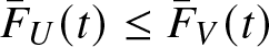
Example 3.2. Let  $U_i\sim q-W(q, \lambda_i, \beta)$ and $V_i\sim q-W(q, \lambda_i^\star, \beta), i=1,2$. First, consider he case $0 \lt q \lt 1$ with $q=0.5, \beta=0.5, \lambda_1=0.5, \lambda_2=1.5, \lambda_1^\star= 0.3$, and $\lambda_2^\star = 1.8$. Here $(\lambda_1,\lambda_2)\preceq_w (\lambda_1^\star,\lambda_2^\star)$. Figure 1(a) represents the plot of $\bar{F}_{U_{1:2}}(t)/\bar{F}_{V_{1:2}}(t)$ in $(0,D)=(0,1.23)$. The plot clearly indicates that $\bar{F}_{U_{1:2}}(t)/\bar{F}_{V_{1:2}}(t)$ is increasing in $t$, which in turn implies $h_{U_{1:2}}\leq h_{V_{1:2}}$ and hence $U_{1:2}\geq_{hr} V_{1:2}$. Similarly, for the case of $q \gt 1$, consider $q=1.5, \beta=0.5, \lambda_1=0.6, \lambda_2=1.5, \lambda_1^\star= 0.3$, and $\lambda_2^\star = 1.7$, where $(\lambda_1,\lambda_2)\preceq^w (\lambda_1^\star,\lambda_2^\star)$. Then from Figure 1(b), it is clear that $\bar{F}_{U_{1:2}}(t)/\bar{F}_{V_{1:2}}(t)$ is decreasing in $t$, which leads to $U_{1:2}\leq_{hr} V_{1:2}$.
Plots of  ${\overline F}_{U_{1:2}}(t)/{\overline F}_{V_{1:2}}(t)$: (a) $q=0.5, \beta=0.5, \lambda_1=0.5, \lambda_2=1.5, \lambda_1^\star= 0.3, \lambda_2^\star = 1.8$ and (b) $q=1.5, \beta=0.5, \lambda_1=0.6, \lambda_2=1.5, \lambda_1^\star= 0.3, \lambda_2^\star = 1.7$.

Figure 1 Long description
The image A showing a line graph. The x-axis label is t, ranging from 0.0 to 1.2 with labeled ticks at 0.0, 0.2, 0.4, 0.6, 0.8, 1.0 and 1.2. The y-axis label is F bar subscript U subscript 1 colon 2 of t over F bar subscript V subscript 1 colon 2 of t, ranging from 0 to 50 with labeled ticks at 0, 10, 20, 30, 40 and 50. A single curve starts near y equals 0 at t equals 0.0, increases slowly up to about t equals 0.8, then rises more quickly. The curve passes near y equals 10 at about t equals 1.0, then increases steeply between about t equals 1.0 and t equals 1.2, reaching near y equals 50 close to t equals 1.2. The image B showing a line graph. The x-axis label is t, ranging from 0 to 10000 with labeled ticks at 0, 2000, 4000, 6000, 8000 and 10000. The y-axis label is F bar subscript U subscript 1 colon 2 of t over F bar subscript V subscript 1 colon 2 of t, with labeled ticks at 0.59, 0.60, 0.61, 0.62 and 0.63. A single curve starts near y equals 0.635 at t equals 0, decreases to about y equals 0.605 near t equals 2000, then continues decreasing more gradually. The curve is near y equals 0.595 around t equals 4000, near y equals 0.590 around t equals 6000, near y equals 0.587 around t equals 8000 and near y equals 0.585 at t equals 10000.
Theorem 3.1 demonstrated that under the stated conditions, the smallest order statistics are comparable in hazard rate order. A natural question arises: Does this conclusion hold when substituting the hazard rate order by the likelihood ratio order? The following counterexample furnishes the answer.
Example 3.3. Let  $U_i\sim q-W(q, \lambda_i, \beta)$ and $V_i\sim q-W(q, \lambda_i^\star, \beta), i=1,2$. Choose $q=0.5, \beta=0.5, \lambda_1=0.5, \lambda_2=1.5, \lambda_1^\star= 0.3$, and $\lambda_2^\star = 1.7$. Then, Figure 2(a) represents the plot of $f_{V_{1:2}}(t)/f_{U_{1:2}}(t)$ in a subset of $(0,D)= (0, 1.38)$, from which it is clear that $f_{V_{1:2}}(t)/f_{U_{1:2}}(t)$ is not an increasing function in $t$. Thus, for $0 \lt q \lt 1$, $U_{1:n}$ and $V_{1:n}$ are not comparable in likelihood ratio order when
  $(\lambda_1, \lambda_2) \stackrel{m}\preceq
(\lambda^\star_1, \lambda^\star_2)$. A similar conclusion can also be drawn when
$(\lambda_1, \lambda_2) \stackrel{m}\preceq
(\lambda^\star_1, \lambda^\star_2)$. A similar conclusion can also be drawn when  $q$ is larger than $1$. Set, $q=1.5, \beta=2, \lambda_1=0.5, \lambda_2=1.5, \lambda_1^\star= 0.3$, and $\lambda_2^\star = 1.7$. Then, from Figure 2(b) it is clear that $f_{V_{1:2}}(t)/f_{U_{1:2}}(t)$ is also not an increasing function, which enables us to say that $U_{1:n}$ and $V_{1:n}$ are not comparable in likelihood ratio order.
Plots of  $f_{V_{1:2}}(t)/f_{U_{1:2}}(t)$: (a) $q=0.5, \beta=0.5, \lambda_1=0.5, \lambda_2=1.5, \lambda_1^\star= 0.3, \lambda_2^\star = 1.7$ and (b) $q=1.5, \beta=2, \lambda_1=0.5, \lambda_2=1.5, \lambda_1^\star= 0.3, \lambda_2^\star = 1.7$.

Figure 2 Long description
The graphs show the ratio f subscript V subscript 1 colon 2 (t) over f subscript U subscript 1 colon 2 (t) plotted against time t. No units are shown for t or the ratio. Graph A: The x-axis is labeled t, ranging from 0.0 to 0.4. The y-axis is labeled f subscript V subscript 1 colon 2 (t) over f subscript U subscript 1 colon 2 (t), ranging from 0.99 to 1.02. The curve starts near 1.00, peaks above 1.02 between t equals 0.1 and t equals 0.2, then declines below 0.99 by t equals 0.4. Graph B: The x-axis is labeled t, ranging from 0.0 to 2.0. The y-axis is labeled f subscript V subscript 1 colon 2 (t) over f subscript U subscript 1 colon 2 (t), ranging from 0.96 to 1.04. The curve starts near 1.00, dips slightly above 0.96 around t equals 1.0, then rises above 1.04 by t equals 2.0. Graph A and B represent different parameter settings: A with q equals 0.5, beta equals 0.5, lambda subscript 1 equals 0.5, lambda subscript 2 equals 1.5, lambda subscript 1 star equals 0.3, lambda subscript 2 star equals 1.7; B with q equals 1.5, beta equals 2, lambda subscript 1 equals 0.5, lambda subscript 2 equals 1.5, lambda subscript 1 star equals 0.3, lambda subscript 2 star equals 1.7. The graphs illustrate how the ratio changes under these conditions, with A showing an early peak and decline, while B shows a dip and subsequent rise.
Theorem 3.4. Let  $U_1, U_2, \ldots, U_n$ be a set of independent r.v.’s such that $U_i\sim$ q-W $(q_i,\lambda, \beta)$, $i= 1,2,\ldots, n$, and $V_1, V_2, \ldots, V_n$ be another set of independent r.v.’s such that $V_i\sim$ q-W $(q^{\star}_i,\lambda, \beta)$, $i= 1,2,\ldots, n$. Then the following results hold:
(1) If
$0 \lt \max_l\{q_l,q^{\star}_l\} \lt 1$ and
$(q_1, q_2, \ldots, q_n)\preceq^{w}(q^{\star}_1, q^{\star}_2, \ldots, q^{\star}_n)$, then
$V_{1:n}\leq_{hr}U_{1:n}$.(2) If
$1 \lt \min_l\{q_l,q^{\star}_l\} \lt 2$ and
$(q_1, q_2, \ldots, q_n)\preceq^{w}(q^{\star}_1, q^{\star}_2, \ldots, q^{\star}_n)$, then
$V_{1:n}\leq_{hr}U_{1:n}.$


Proof. The results can be established following arguments similar to those used in Theorem 3.1.
We now present a numerical example to illustrate the result established in Theorem 3.4.
Example 3.5. Let  $U_i\sim q-W(q_i, \lambda, \beta)$ and $V_i\sim q-W(q^\star_i, \lambda_i, \beta), i=1,2$. For the case $q \lt 1$, consider $q_1=0.3, q_2=0.5, q_1^\star=0.1, q_2^\star=0.6,\beta=2$, and $ \lambda=0.5$, where $(q_1,q_2)\preceq^w (q_1^\star,q_2^\star)$. Figure 3(a) displays the plot of $\bar{F}_{U_{1:2}}(t)/\bar{F}_{V_{1:2}}(t)$ over the interval $(0,D)=(0,1.49)$. The figure clearly shows that $\bar{F}_{U_{1:2}}(t)/\bar{F}_{V_{1:2}}(t)$ is increasing function in $t$, which implies that $U_{1:2}\geq_{hr} V_{1:2}$. Similarly, for the case of $q \gt 1$, let $q_1=1.3, q_2=1.5, q_1^\star=1.1, q_2^\star=1.6,\beta=2$, and $\lambda=0.5$, with $(q_1,q_2)\preceq^w (q_1^\star,q_2^\star)$. As illustrated in Figure 3(b), $\bar{F}_{U_{1:2}}(t)/\bar{F}_{V_{1:2}}(t)$ is again increasing, confirming that, $U_{1:2}\geq_{hr} V_{1:2}$.
Plots of  $\bar{F}_{U_{1:2}}(t)/\bar{F}_{V_{1:2}}(t)$: (a) $q_1=0.3, q_2= 0.5, q_1^\star=0.1, q_2^\star= 0.6, \beta=2, \lambda = 0.5$ and (b) $q_1=1.3, q_2= 1.5, q_1^\star=1.1, q_2^\star= 1.6, \beta=2, \lambda = 0.5$.

Figure 3 Long description
The image A showing a line graph. Vertical axis label: F bar subscript U subscript 1 colon 2 left parenthesis t right parenthesis over F bar subscript V subscript 1 colon 2 left parenthesis t right parenthesis. Vertical axis range: 0 to 50. Horizontal axis label: t. Horizontal axis range: 0.0 to 1.5. Plotted line: starts near 0 at t equals 0.0, stays near 0 up to about t equals 1.2, rises to about 1 at about t equals 1.3, rises to about 5 at about t equals 1.4 and rises steeply to about 50 near t equals 1.5. Text below the graph: left parenthesis a right parenthesis q subscript 1 equals 0.3, q subscript 2 equals 0.5, q subscript 1 star equals 0.1, q subscript 2 star equals 0.6, beta equals 2, lambda equals 0.5. The image B showing a line graph. Vertical axis label: F bar subscript U subscript 1 colon 2 left parenthesis t right parenthesis over F bar subscript V subscript 1 colon 2 left parenthesis t right parenthesis. Vertical axis range: 0 to 2.5 times 10 superscript 42. Horizontal axis label: t. Horizontal axis range: 0 to 10000. Plotted line: starts near 0 at t equals 0, stays near 0 up to about t equals 6000, rises to about 5.0 times 10 superscript 41 at about t equals 8000, rises to about 1.0 times 10 superscript 42 at about t equals 8500, rises to about 1.5 times 10 superscript 42 at about t equals 9000, rises to about 2.0 times 10 superscript 42 at about t equals 9500 and reaches about 2.5 times 10 superscript 42 near t equals 10000. Text below the graph: left parenthesis b right parenthesis q subscript 1 equals 1.3, q subscript 2 equals 1.5, q subscript 1 star equals 1.1, q subscript 2 star equals 1.6, beta equals 2, lambda equals 0.5.
The above theorem establishes the comparison result with respect to the hazard rate order. A natural question is whether this conclusion also holds when the hazard rate order is replaced by the likelihood ratio order. The following counterexample provides an answer.
Example 3.6. Let  $U_i\sim q-W(q_i, \lambda, \beta)$ and $V_i\sim q-W(q_i^\star, \lambda, \beta), i=1,2$. Choose $q_1=0.2, q_2= 0.7, q_1^\star=0.1, q_2^\star= 0.8, \beta=2$, and $ \lambda = 0.5$. Then,
  $(q_1, q_2) \stackrel{m}\preceq
(q^\star_1, q^\star_2)$. Figure 4(a) represents the plot of
$(q_1, q_2) \stackrel{m}\preceq
(q^\star_1, q^\star_2)$. Figure 4(a) represents the plot of  $f_{V_{1:2}}(t)/f_{U_{1:2}}(t)$ in a subset of $(0,D)= (0, 1.49)$, from which it is clear that $f_{V_{1:2}}(t)/f_{U_{1:2}}(t)$ is not an increasing function in $t$. Thus, for $0 \lt \max_l\{q_l,q^{\star}_l\} \lt 1$, $U_{1:n}$ and $V_{1:n}$ are not comparable in likelihood ratio order. By setting, $q_1=1.2, q_2= 1.7, q_1^\star=1.1, q_2^\star= 1.8, \beta=2$, and $ \lambda = 0.5$ similar, conclusion can also be drawn from Figure 4(b), when $1 \lt \min_l\{q_l,q^{\star}_l\} \lt 2$.
Plots of  $f_{V_{1:2}}(t)/f_{U_{1:2}}(t)$: (a) $q_1=0.2, q_2= 0.7, q_1^\star=0.1, q_2^\star= 0.8, \beta=2, \lambda = 0.5$ and (b) $q_1=1.2, q_2= 1.7, q_1^\star=1.1, q_2^\star= 1.8, \beta=2, \lambda = 0.5$.

Figure 4 Long description
The image contains two line graphs. The first graph shows the ratio of functions f subscript V subscript 1 colon 2 (t) over f subscript U subscript 1 colon 2 (t) on the vertical axis, ranging from 1.000 to 1.015, against time t on the horizontal axis, ranging from 0 to 1.5. Parameters are q subscript 1 equals 0.2, q subscript 2 equals 0.7, q subscript 1 superscript star equals 0.1, q subscript 2 superscript star equals 0.8, beta equals 2, lambda equals 0.5. The graph shows an increasing trend peaking around t equals 1. The second graph has the same vertical axis and time t on the horizontal axis, ranging from 0 to 1.5. Parameters are q subscript 1 equals 1.2, q subscript 2 equals 1.7, q subscript 1 superscript star equals 1.1, q subscript 2 superscript star equals 1.8, beta equals 2, lambda equals 0.5. This graph also shows an increasing trend with a peak around t equals 1. Both graphs illustrate how changes in parameters affect the function ratio over time.
Next, we consider the case when heterogeneity occurs in terms of the parameter  $\beta$.
Theorem 3.7. Let  $U_1, U_2, \ldots, U_n$ be a set of independent r.v.’s such that $U_i\sim$ q-W $(q,\lambda, \beta_i)$, $i= 1,2,\ldots, n$, and $V_1, V_2, \ldots, V_n$ be another set of independent r.v.’s such that $V_i\sim$ q-W $(q,\lambda, \beta^{\star}_i)$, $i= 1,2,\ldots, n$. Then the following results hold:
(1) If
$0 \lt q \lt 1$ and
$(\beta_1, \beta_2, \ldots, \beta_n) \stackrel{m}\preceq (\beta^{\star}_1, \beta^{\star}_2, \ldots, \beta^{\star}_n)$, then
$V_{1:n}\leq_{st}U_{1:n}$.(2) If
$1 \lt q \lt 2$ and
$(\beta_1, \beta_2, \ldots, \beta_n) \stackrel{m}\preceq (\beta^{\star}_1, \beta^{\star}_2, \ldots, \beta^{\star}_n)$, then
$V_{1:n}\leq_{st}U_{1:n}.$


(1) To establish the theorem, it suffices to show that
$\bar{F}_{U_{1:n}}(t)\leq \bar{F}_{V_{1:n}}(t)$ for all
$t\in (0, D)$, where
$\bar{F}_{U_{1:n}}(t)$ and
$\bar{F}_{V_{1:n}}(t)$ denote the survival functions of
$U_{1:n}$ and
$V_{1:n}$, as defined in (2) and (3), respectively. Note that
where
\begin{equation*}\bar{F}_{U_{1:n}}(t)=\prod_{l=1}^n\bar{F}_{U_l}(t):=\prod_{l=1}^{n}\eta(\beta_l),\end{equation*}
$\eta(x)=\left[1-\lambda(1-q)t^{x}\right]^{\frac{2-q}{1-q}}$. By Proposition E.1 of [Reference Marshall, Olkin and Arnold32], it is sufficient to show that
$\ln{(\eta(x))}$ is concave in
$x$. Observe that for all
$t\in D$,
as for all
\begin{equation*}\dfrac{d^2}{dx^2}\ln(\eta(x)) = \dfrac{-(2-q)\lambda t^x (\ln(t))^2}{[1-(1-q)\lambda t^x]^2}\leq 0,\end{equation*}
$\beta_l$,
$0 \lt t \lt D\Rightarrow 0 \lt t \lt \min_{l}\left\lbrace \lambda(1-q)]^{-\frac{1}{\beta_l}}\right\rbrace$. Therefore,
$\bar{F}_{1:n}(t)$ is Schur-concave in
$(\beta_1,\beta_2, \ldots,\beta_n)$. Hence, the result follows.(2) By a similar argument, the proof of this part follows from the observation that for all
$t$,
$\frac{d^2}{dx^2}\ln(\eta(x))\leq 0.$


A numerical example is provided below to illustrate Theorem 3.7.
Example 3.8. Let  $U_i\sim q-W(q, \lambda, \beta_i)$ and $V_i\sim q-W(q, \lambda_i, \beta^\star_i), i=1,2$. For the case $q \lt 1$, consider $q=0.5,\beta_1=0.5,\beta_2=1.5, \beta_1^\star=0.3, \beta_2^\star=1.7$, and $\lambda=1$, where $(\beta_1,\beta_2) \stackrel{m}\preceq (\beta_1^\star,\beta_2^\star)$. Figure 5(a) shows the plot of $\bar{F}_{U_{1:2}}(t)-\bar{F}_{V_{1:2}}(t)$ in the interval $(0,D)=(0,1.5)$. It is evident from the figure that $\bar{F}_{U_{1:2}}(t)-\bar{F}_{V_{1:2}}(t)\geq 0$ for all $t$, which implies that $U_{1:2}\geq_{st} V_{1:2}$. Similarly, for the case of $q \gt 1$, take $q=1.5,\beta_1=0.5,\beta_2=1.5, \beta_1^\star=0.3, \beta_2^\star=1.7$, and $ \lambda=0.5$, with $(\beta_1,\beta_2) \stackrel{m}\preceq (\beta_1^\star,\beta_2^\star)$. As illustrated in Figure 6(b), $\bar{F}_{U_{1:2}}-\bar{F}_{V_{1:2}}\geq 0$, confirming that $U_{1:2}\geq_{st} V_{1:2}$.
Plots of  $\bar{F}_{U_{1:2}}(t)-\bar{F}_{V_{1:2}}(t)$: (a) $q=0.5,\beta_1=0.5,\beta_2=1.5, \beta_1^\star=0.3, \beta_2^\star=1.7, \lambda = 1$ and (b) $q=1.5,\beta_1=0.5,\beta_2=1.5, \beta_1^\star=0.3, \beta_2^\star=1.7, \lambda = 0.5$.

Figure 5 Long description
Two separate line plots are shown side by side, labeled as panel a and panel b. Both plots display the difference F bar subscript U subscript 1 colon 2 of t minus F bar subscript V subscript 1 colon 2 of t on the y-axis, where F bar denotes a survival function and U subscript 1 colon 2 and V subscript 1 colon 2 denote minimum order statistics from two groups of components. The x-axis in both panels is labeled t, with no units indicated. Panel a uses the parameter values q equals 0.5, beta subscript 1 equals 0.5, beta subscript 2 equals 1.5, beta subscript 1 star equals 0.3, beta subscript 2 star equals 1.7 and lambda equals 1. The x-axis ranges from 0.0 to 1.5 and the y-axis ranges from 0.00 to 0.20. The curve starts near 0.00 at t equals 0.0, rises steeply to a peak of approximately 0.20 near t equals 0.05, then decreases continuously. At t equals 0.2 the value is near 0.11, at t equals 0.4 near 0.04, at t equals 0.6 near 0.01, at t equals 0.8 near 0.00 and the curve remains at approximately 0.00 from t equals 1.0 through t equals 1.5. Panel b uses the parameter values q equals 1.5, beta subscript 1 equals 0.5, beta subscript 2 equals 1.5, beta subscript 1 star equals 0.3, beta subscript 2 star equals 1.7 and lambda equals 0.5. The x-axis ranges from 0 to 1000 and the y-axis ranges from 0.00000 to 0.00030. The curve begins at its highest value near 0.00029 close to t equals 0 and decreases monotonically without a visible interior peak. At t equals 200 the value is near 0.00010, at t equals 400 near 0.00003, at t equals 600 near 0.00001 and from t equals 800 onward the curve remains at approximately 0.00000. The two panels differ in the value of q and lambda and in the x-axis scale and y-axis magnitude, with panel a operating over a short time range with values up to 0.20 and panel b operating over a much longer time range with values up to 0.00030.
The following counterexample illustrates that the condition in Theorem 3.7 is not sufficient for the hazard rate ordering between  $U_{1:n}$ and $V_{1:n}$.
Example 3.9. Let  $U_i\sim q-W(q, \lambda, \beta_i)$ and $V_i\sim q-W(q, \lambda, \beta_i^\star), i=1,2$. Consider $q=0.3, \beta_1=0.5, \beta_2 = 0.5, \beta_1^\star = 0.3, \beta_2^\star = 0.7$, and $ \lambda = 0.5$. From Figure 6(a), it is clear that $\bar{F}_{V_{1:2}}(t)/\bar{F}_{U_{1:2}}(t)$ is not monotone in a subset of $(0, D) = (0, 4.48)$. Then for $0 \lt q \lt 1$, $(\beta_1, \beta_2) \stackrel{m}\preceq (\beta^{\star}_1, \beta^{\star}_2)$ does not imply $V_{1:n}\leq_{hr}U_{1:n}.$ Similarly, taking, $q=1.3, \beta_1=0.5, \beta_2 = 0.5, \beta_1^\star = 0.3, \beta_2^\star = 0.7$, and $ \lambda = 0.5$ we can conclude from Figure 6(b) that $U_{1:n}$ and $V_{1:n}$ are not comparable in hazard rate order when $1 \lt q \lt 2$ and $(\beta_1, \beta_2) \stackrel{m}\preceq (\beta^{\star}_1, \beta^{\star}_2)$.
Plots of  $\bar{F}_{V_{1:2}}(t)/\bar{F}_{U_{1:2}}(t)$: (a) $q=0.3, \beta_1=0.5, \beta_2 = 0.5, \beta_1^\star = 0.3, \beta_2^\star = 0.7, \lambda = 0.5$ and (b) $q=1.3, \beta_1=0.5, \beta_2 = 0.5, \beta_1^\star = 0.3, \beta_2^\star = 0.7, \lambda = 0.5$.

Figure 6 Long description
The image A showing a line graph. Horizontal axis label: t. Horizontal axis range: 0.0 to 1.5. Vertical axis label: F bar subscript V subscript 1 colon 2 of t over F bar subscript U subscript 1 colon 2 of t. Vertical axis range: 0.93 to 1.00. Plotted coordinate pairs: (0.1, 0.93), (0.2, 0.95), (0.4, 0.97), (0.6, 0.99), (1.0, 1.00), (1.5, 0.98). Lowest listed point: (0.1, 0.93). Highest listed point: (1.0, 1.00). Curve shape from listed points: increases from t equals 0.1 to t equals 1.0, then decreases from t equals 1.0 to t equals 1.5. The image B showing a line graph. Horizontal axis label: t. Horizontal axis range: 0.0 to 1.5. Vertical axis label: F bar subscript V subscript 1 colon 2 of t over F bar subscript U subscript 1 colon 2 of t. Vertical axis range: 0.93 to 1.00. Plotted coordinate pairs: (0.1, 0.97), (0.3, 1.00), (0.6, 0.99), (1.0, 0.97), (1.5, 0.93). Lowest listed point: (1.5, 0.93). Highest listed point: (0.3, 1.00). Curve shape from listed points: increases from t equals 0.1 to t equals 0.3, then decreases from t equals 0.3 to t equals 1.5. Comparison using listed points: the highest listed value is 1.00 in both images, occurring at t equals 1.0 in image A and at t equals 0.3 in image B. From t equals 1.0 to t equals 1.5, image A changes from 1.00 to 0.98 and image B changes from 0.97 to 0.93.
Next, we carry out stochastic comparisons between the largest order statistics arising from two sets of heterogeneous  $q$-Weibull samples $U_i$’s and $V_i$’s with parameters $(q_i,\lambda_i, \beta_i)$ and $(q_i^{\star},\lambda^{\star}_i, \beta_i^{\star})$, $i= 1,2,\ldots, n$, respectively. Suppose ${F}_{U_{n:n}}(t)$ and ${F}_{V_{n:n}}(t)$ are the d.f.’s of the largest order statistics $U_{n:n}$ and $V_{n:n}$, respectively, then
 \begin{equation*}{F}_{U_{n:n}}(t) = \prod_{l=1}^{n}{F}_{U_l}(t)= \prod_{l=1}^{n}\left[1-\left[1-\lambda_l(1-q_l)t^{\beta_l}\right]^{\frac{2-q_l}{1-q_l}}\right],\end{equation*}
and
 \begin{equation*}{F}_{V_{n:n}}(t) =\prod_{l=1}^{n}{F}_{V_l}(t)= \prod_{l=1}^{n}\left[1-\left[1-\lambda_l^{\star}(1-q_l^{\star})t^{\beta_l^{\star}}\right]^{\frac{2-q_l^{\star}}{1-q_l^{\star}}}\right].\end{equation*}
 It is important to note that, for  $0 \lt q_l, q^*_l \lt 1$, $X_{n:n}$ and $Y_{n:n}$ are defined over different domains. So, for any comparison of these r.v.’s, we should take the common domain of $U_{n:n}$ and $V_{n:n}$ as $(0, D)$ where
  $D= \min\left\lbrace\min_l\left\lbrace[\lambda_l(1-q_l)]^{-\frac{1}{\beta_l}} \right\rbrace,
\min_{l}\left\lbrace[\lambda^{*}_l(1-q^{*}_l)]^{-\frac{1}{\beta^{*}_l}} \right\rbrace\right\rbrace$.
$D= \min\left\lbrace\min_l\left\lbrace[\lambda_l(1-q_l)]^{-\frac{1}{\beta_l}} \right\rbrace,
\min_{l}\left\lbrace[\lambda^{*}_l(1-q^{*}_l)]^{-\frac{1}{\beta^{*}_l}} \right\rbrace\right\rbrace$.
Theorem 3.10. Let  $U_1, U_2, \ldots, U_n$ be a set of independent r.v.’s such that $U_i\sim$ q-W $(q,\lambda_i, \beta)$, $i= 1,2,\ldots, n$, and $V_1, V_2, \ldots, V_n$ be another set of independent r.v.’s such that $V_i\sim$ q-W $(q,\lambda^{*}_i, \beta)$, $i= 1,2,\ldots, n$. Then the following results hold:
(1) If
$0 \lt q \lt 1$ and
$(\lambda_1, \lambda_2, \ldots, \lambda_n)\preceq^{w}(\lambda^{*}_1, \lambda^{*}_2, \ldots, \lambda^{*}_n)$, then
$U_{n:n}\leq_{st}V_{n:n}$.(2) If
$1 \lt q \lt 2$ and
$(\lambda_1, \lambda_2, \ldots, \lambda_n){\preceq^{w}}(\lambda^{*}_1, \lambda^{*}_2, \ldots, \lambda^{*}_n)$, then
$U_{n:n}\leq_{st}V_{n:n}$.


Proof. The d.f. of the largest order statistics  $U_{n:n}$ can be written as
 \begin{equation*}{F}_{U_{n:n}}(t) = \prod_{l=1}^{n}\left[1-\left[1-\lambda_l(1-q_l)t^\beta\right]^{\frac{2-q}{1-q}}\right] = \prod_{l=1}^{n} \xi_t(\lambda_l).\end{equation*}
Now we have
 \begin{equation*}\dfrac{d}{d\lambda}ln[\xi_t(\lambda)]= (2-q)t^{\beta}\dfrac{\left[1-\lambda(1-q)t^\beta\right]^{\frac{1}{1-q}}}{1-\left[1-\lambda(1-q)t^\beta\right]^{\frac{2-q}{1-q}}}\end{equation*}
and
 \begin{align*}
&\dfrac{d^2}{d\lambda^2}ln[\xi_t(\lambda)]\stackrel{sign}=-(2-q)\left(1-\lambda(1-q)t^\beta\right)^{\frac{1}{1-q}}\\
&\quad\times
\left[ \left(1-\lambda(1-q)t^\beta\right)^{-1}\lbrace1-\left(1-\lambda(1-q)t^\beta\right)^{\frac{2-q}{1-q}}\rbrace+(2-q)\left(1-\lambda(1-q)t^\beta\right)^{\frac{1}{1-q}}\right].
\end{align*}
\begin{align*}
&\dfrac{d^2}{d\lambda^2}ln[\xi_t(\lambda)]\stackrel{sign}=-(2-q)\left(1-\lambda(1-q)t^\beta\right)^{\frac{1}{1-q}}\\
&\quad\times
\left[ \left(1-\lambda(1-q)t^\beta\right)^{-1}\lbrace1-\left(1-\lambda(1-q)t^\beta\right)^{\frac{2-q}{1-q}}\rbrace+(2-q)\left(1-\lambda(1-q)t^\beta\right)^{\frac{1}{1-q}}\right].
\end{align*}(1) To prove the result using Lemma 2.4, we need the Schur-concavity of
${F}_{n:n}(t)$ in
$\lambda$. By Proposition E.1. of [Reference Marshall, Olkin and Arnold32], this can be shown by the concavity property of
$ ln[\xi_t(\lambda_l)]$ in
$\lambda$. Now, for
$0 \lt q \lt 1$, we have
$0\leq t\leq D$, which implies
$\dfrac{d}{d\lambda}ln[\xi_t(\lambda)]\geq 0$ and
$\dfrac{d^2}{d\lambda^2}ln[\xi_t(\lambda)]\leq 0$. Hence, the result follows.(2) For
$1 \lt q \lt 2$, we similarly obtain
$\dfrac{d}{d\lambda}ln[\xi_t(\lambda)]\geq 0$ and
$\dfrac{d^2}{d\lambda^2}ln[\xi_t(\lambda)]\leq 0,$ which again implies the Schur-concavity of
${F}_{U_{n:n}}(t)$ by Proposition E.1. of [Reference Marshall, Olkin and Arnold32]. The conclusion then follows from Lemma 2.4.


Below, we consider a numerical example to demonstrate the result stated in Theorem 3.10.
Example 3.11. Let  $U_i\sim q-W(q, \lambda_i, \beta)$ and $V_i\sim q-W(q, \lambda_i^\star, \beta), i=1,2$. For the case $q \lt 1$, consider $q=0.5, \beta=0.5, \lambda_1=0.5, \lambda_2=1.5, \lambda_1^\star= 0.3$, and $\lambda_2^\star = 1.6$, where $(\lambda_1,\lambda_2)\preceq^w (\lambda_1^\star,\lambda_2^\star)$. Figure 7(a) presents the plot of ${F}_{U_{2:2}}(t)-{F}_{V_{2:2}}(t)$ in the interval $(0,D)=(0,1.56)$. The plot clearly indicates that ${F}_{U_{2:2}}(t)-{F}_{V_{2:2}}(t)\geq 0$ in $t$, which implies $U_{2:2}\leq_{st} V_{2:2}$. Similarly, for the case of $q \gt 1$, choose $q=1.5, \beta=0.5, \lambda_1=0.5, \lambda_2=1.5, \lambda_1^\star= 0.3$, and $\lambda_2^\star = 1.6$, with $(\lambda_1,\lambda_2)\preceq^w (\lambda_1^\star,\lambda_2^\star)$. As shown in Figure 7(b), we again find that ${F}_{U_{2:2}}(t)-{F}_{V_{2:2}}(t)\geq 0$, confirming that, $U_{2:2}\leq_{st} V_{2:2}$.
Plots of  ${F}_{U_{2:2}}(t)-{F}_{V_{2:2}}(t)$: (a) $q=0.5, \beta=0.5, \lambda_1=0.5, \lambda_2=1.5, \lambda_1^\star= 0.3,\lambda_2^\star = 1.6$ and (b) $q=1.5, \beta=0.5, \lambda_1=0.5, \lambda_2=1.5, \lambda_1^\star= 0.3,\lambda_2^\star = 1.6$.

Figure 7 Long description
The image consists of two panels, A and B, each showing a line graph. Panel A: The vertical axis represents F subscript U subscript m colon n of t minus F subscript V subscript m colon n of t, ranging from 0.00 to 0.20. The horizontal axis represents t, ranging from 0.0 to 1.5. The graph features a single orange solid line that rises quickly and plateaus near 0.21 by t equals 1.5. The parameters are q equals 0.5, beta equals 0.5, lambda subscript 1 equals 0.5, lambda subscript 2 equals 1.5, lambda subscript 1 star equals 0.3 and lambda subscript 2 star equals 1.6. Panel B: The vertical axis represents F subscript U subscript m colon n of t minus F subscript V subscript m colon n of t, ranging from 0.00 to 0.06. The horizontal axis represents t, ranging from 0 to 10000. The graph features a single orange solid line that starts near 0.07 and decays toward 0.02 by t equals 10000. The parameters are q equals 1.5, beta equals 0.5, lambda subscript 1 equals 0.5, lambda subscript 2 equals 1.5, lambda subscript 1 star equals 0.3 and lambda subscript 2 star equals 1.6. The graphs illustrate the behavior of the function under different parameter settings, with Panel A showing a rapid increase and leveling off, while Panel B shows a gradual decay.
4. Heterogeneous dependent samples
In this section, we compare the extreme order statistics coming from the r.v.’s  $U_1, U_2, \ldots, U_n$ and $V_1, V_2, \ldots, V_n$ having distribution functions $F_{U_i} (\cdot)$ and $F_{V_i}(\cdot)$, respectively. We consider that these random variables are dependent, and the dependence structure is modeled by an Archimedean copula.
Let us consider two sets of heterogeneous  $q$-Weibull samples, $U_i$’s and $V_i$’s, with parameters $(q_i,\lambda_i, \beta_i)$ and $(q_i^{\star},\lambda^{\star}_i, \beta_i^{\star})$, $i= 1,2,\ldots, n$, respectively. The dependence structures of these samples are modeled by Archimedean copulas with generators $\psi_1 (\phi_1= \psi_1^{-1})$ and $\psi_2 (\phi_2= \psi_2^{-1})$. As discussed earlier, for comparison results in case of $0 \lt q_i,q_i^\star \lt 1$, we should take the common domain of $U_{n:n}$ and $V_{n:n}$ as $(0, D)$, where
  $D= \min\left\lbrace\min_i\left\lbrace[\lambda_i(1-q_i)]^{-\frac{1}{\beta_i}} \right\rbrace,
\min_{i}\left\lbrace[\lambda^{\star}_i(1-q^{\star}_i)]^{-\frac{1}{\beta^{\star}_i}} \right\rbrace\right\rbrace$.
$D= \min\left\lbrace\min_i\left\lbrace[\lambda_i(1-q_i)]^{-\frac{1}{\beta_i}} \right\rbrace,
\min_{i}\left\lbrace[\lambda^{\star}_i(1-q^{\star}_i)]^{-\frac{1}{\beta^{\star}_i}} \right\rbrace\right\rbrace$.
Theorem 4.1. Let  $U_i \sim q-W(q,\lambda_i, \beta)$, $i=1, ...,n$, be a set of dependent r.v.’s sharing an Archimedean copula with generator $\psi_1$. Similarly, let $V_i \sim q-W(q,\lambda^\star_i, \beta)$, $i=1, ...,n$, be a set of dependent r.v.’s sharing an Archimedean copula with generator $\psi_2$.
(1) Suppose that
$\phi_2 \circ \psi_1$ is super-additive and
$\psi_1$ or
$\psi_2$ is log-convex. Then, for
$0 \lt q \lt 1$ and
$\boldsymbol{{\lambda}}\in \mathbb{D}_+(\mathbb{E}_+)$,
\begin{equation*}(\lambda^{\star}_1, \lambda^{\star}_2, \ldots, \lambda^{\star}_n)\preceq^{w}(\lambda_1, \lambda_2, \ldots, \lambda_n)\,\, \textit{implies}\,\, U_{n:n}\geq_{st}V_{n:n}.\end{equation*}(2) Suppose that
$\phi_2 \circ \psi_1$ is super-additive and
$\psi_1$ or
$\psi_2$ is log-convex. Then, for
$1 \lt q \lt 2$ and
$\boldsymbol{{\lambda}}\in \mathbb{D}_+(\mathbb{E}_+)$,
\begin{equation*}(\lambda^{\star}_1, \lambda^{\star}_2, \ldots, \lambda^{\star}_n)\preceq^{w} (\lambda_1, \lambda_2, \ldots, \lambda_n)\,\,\textit{implies}\,\, U_{n:n}\geq_{st}V_{n:n}.\end{equation*}


Proof. The d.f.s of  $X_{n:n}$ and $Y_{n:n}$ can be written as follows
 \begin{equation*}F_{U_{n:n}}(t) = \psi_1\left[\sum_{i=1}^{n} \phi_1\left[1-(1-\lambda_i(1-q)t^{\beta})^{\frac{2-q}{1-q}}\right]\right],\end{equation*}
and
 \begin{equation*}F_{V_{n:n}}(t) = \psi_2\left[\sum_{i=1}^{n} \phi_2\left[1-(1-\lambda^*_i(1-q)t^{\beta})^{\frac{2-q}{1-q}}\right]\right].\end{equation*}
 Since  $\phi_2 \circ \psi_1$ is assumed to be super-additive, it follows from Lemma 2.7 that
 \begin{equation}
\psi_1\left[\sum_{i=1}^{n} \phi_1\left[1-(1-\lambda_i(1-q)t^{\beta})^{\frac{2-q}{1-q}}\right]\right]\leq\psi_2\left[\sum_{i=1}^{n} \phi_2\left[1-(1-\lambda_i(1-q)t^{\beta})^{\frac{2-q}{1-q}}\right]\right].
\end{equation}
\begin{equation}
\psi_1\left[\sum_{i=1}^{n} \phi_1\left[1-(1-\lambda_i(1-q)t^{\beta})^{\frac{2-q}{1-q}}\right]\right]\leq\psi_2\left[\sum_{i=1}^{n} \phi_2\left[1-(1-\lambda_i(1-q)t^{\beta})^{\frac{2-q}{1-q}}\right]\right].
\end{equation} Define  $\Omega(\boldsymbol{\lambda})= \psi_2\left[\sum_{i=1}^{n} \phi_2\left[1-(1-\lambda_i(1-q)t^{\beta})^{\frac{2-q}{1-q}}\right]\right]$. Differentiating $\Omega(\boldsymbol{\lambda})$ with respect to $\lambda_k$, we obtain
 \begin{align}
\frac{\partial\Omega(\boldsymbol{\lambda})}{\partial\lambda_k} & = \psi_2^{'}\left[\sum_{i=1}^{n} \phi_2\left[1-(1-\lambda_i(1-q)t^{\beta})^{\frac{2-q}{1-q}}\right]\right]\phi_2^{'}\left[1-(1-\lambda_k(1-q)t^{\beta})^{\frac{2-q}{1-q}}\right]\nonumber\\
&\quad \times(2-q)(1-\lambda_k(1-q)t^{\beta})^{\frac{1}{1-q}}t^{\beta}\nonumber\\
& = \frac{(2-q)t^{\beta}(1-\lambda_k(1-q)t^{\beta})^{\frac{1}{1-q}}}{1-(1-\lambda_k(1-q)t^{\beta})^{\frac{2-q}{1-q}}}\psi_2^{'}\left[\sum_{i=1}^{n} \phi_2\left[1-(1-\lambda_i(1-q)t^{\beta})^{\frac{2-q}{1-q}}\right]\right]\nonumber\\
&\quad \times\frac{\psi_2\left[\phi_2\left[1-(1-\lambda_k(1-q)t^{\beta})^{\frac{2-q}{1-q}}\right]\right]}{\psi_2^{'}\left[ \phi_2\left[1-(1-\lambda_k(1-q)t^{\beta})^{\frac{2-q}{1-q}}\right]\right]}\nonumber\\
\end{align}
\begin{align}
\frac{\partial\Omega(\boldsymbol{\lambda})}{\partial\lambda_k} & = \psi_2^{'}\left[\sum_{i=1}^{n} \phi_2\left[1-(1-\lambda_i(1-q)t^{\beta})^{\frac{2-q}{1-q}}\right]\right]\phi_2^{'}\left[1-(1-\lambda_k(1-q)t^{\beta})^{\frac{2-q}{1-q}}\right]\nonumber\\
&\quad \times(2-q)(1-\lambda_k(1-q)t^{\beta})^{\frac{1}{1-q}}t^{\beta}\nonumber\\
& = \frac{(2-q)t^{\beta}(1-\lambda_k(1-q)t^{\beta})^{\frac{1}{1-q}}}{1-(1-\lambda_k(1-q)t^{\beta})^{\frac{2-q}{1-q}}}\psi_2^{'}\left[\sum_{i=1}^{n} \phi_2\left[1-(1-\lambda_i(1-q)t^{\beta})^{\frac{2-q}{1-q}}\right]\right]\nonumber\\
&\quad \times\frac{\psi_2\left[\phi_2\left[1-(1-\lambda_k(1-q)t^{\beta})^{\frac{2-q}{1-q}}\right]\right]}{\psi_2^{'}\left[ \phi_2\left[1-(1-\lambda_k(1-q)t^{\beta})^{\frac{2-q}{1-q}}\right]\right]}\nonumber\\
\end{align}(1) For
$0 \lt q \lt 1$, we have
$\frac{\partial\Omega(\boldsymbol{\lambda})}{\partial\lambda_k} \geq 0$ when
$t \in [0,D)$, that is,
$\Omega(\boldsymbol{\lambda})$ is increasing in
$\boldsymbol{\lambda}$. Suppose
$\boldsymbol{\lambda} \in \mathbb{D}_+(\mathbb{E}_+)$, that is, for
$i\leq j$,
$\lambda_i \geq (\leq)\lambda_j$ implies
$(1-\lambda_i(1-q)t^{\beta})^{\frac{1}{1-q}}\leq (\geq) (1- \lambda_j (1-q) t^{\beta})^{\frac{1}{1-q}}$, and
$(1-\lambda_i(1-q)t^{\beta})^{\frac{2-q}{1-q}} \leq (\geq)(1-\lambda_j(1-q)t^{\beta})^{\frac{2-q}{1-q}}$. This further implies
(10)since\begin{equation}
\phi_2\left[1-(1-\lambda_i(1-q)t^{\beta})^{\frac{2-q}{1-q}}\right]\leq(\geq)\phi_2\left[1-(1-\lambda_j(1-q)t^{\beta})^{\frac{2-q}{1-q}}\right],
\end{equation}
$\phi_2$ is
$d$-monotone. Now, from our assumption that
$\psi_2$ is log-convex, we can say that
$\frac{\psi_2(t)}{\psi_2^{'}(t)}$ is decreasing in
$t$. Therefore,
(11)\begin{equation}
\frac{\psi_2\left[\phi_2\left[1-(1-\lambda_i(1-q)t^{\beta})^{\frac{2-q}{1-q}}\right]\right]}{\psi_2^{'}\left[ \phi_2\left[1-(1-\lambda_i(1-q)t^{\beta})^{\frac{2-q}{1-q}}\right]\right]}\geq(\leq)\frac{\psi_2\left[\phi_2\left[1-(1-\lambda_j(1-q)t^{\beta})^{\frac{2-q}{1-q}}\right]\right]}{\psi_2^{'}\left[ \phi_2\left[1-(1-\lambda_j(1-q)t^{\beta})^{\frac{2-q}{1-q}}\right]\right]}.
\end{equation}Furthermore, since
$\psi_2$ is
$d$-monotone, it follows that
(12)\begin{align}
& \frac{(2-q)t^{\beta}(1-\lambda_i(1-q)t^{\beta})^{\frac{1}{1-q}}}{1-(1-\lambda_i(1-q)t^{\beta})^{\frac{2-q}{1-q}}}\psi_2^{'}\left[\sum_{i=1}^{n} \phi_2\left[1-(1-\lambda_i(1-q)t^{\beta})^{\frac{2-q}{1-q}}\right]\right]\geq(\leq)\nonumber\\
& \frac{(2-q)t^{\beta}(1-\lambda_j(1-q)t^{\beta})^{\frac{1}{1-q}}}{1-(1-\lambda_j(1-q)t^{\beta})^{\frac{2-q}{1-q}}}\psi_2^{'}\left[\sum_{i=1}^{n} \phi_2\left[1-(1-\lambda_i(1-q)t^{\beta})^{\frac{2-q}{1-q}}\right]\right]\nonumber\\
\end{align}Multiplying (11) and (12), and using (9), we obtain
\begin{equation*}\frac{\partial\Omega(\boldsymbol{\lambda})}{\partial\lambda_i}\leq(\geq)\frac{\partial(\Omega\boldsymbol{\lambda})}{\partial\lambda_j}.\end{equation*}Finally, by Lemma 2 (Lemma 3) of [Reference Kundu, Chowdhury and Balakrishnan28], it follows that
$\Omega(\boldsymbol{\lambda})$ is Schur-concave in
$\boldsymbol{\lambda}$. Combining this with the fact that
$\Omega(\boldsymbol{\lambda})$ is increasing and Schur-concave in
$\boldsymbol{\lambda}$, we obtain the desired result from (8) and Lemma 2.4.(2) For
$1 \lt q \lt 2$, we have
$\frac{\partial\Omega(\boldsymbol{\lambda})}{\partial\lambda_k} \geq 0$ for all
$t \geq 0$, that is,
$\Omega(\boldsymbol{\lambda})$ is increasing in
$\boldsymbol{\lambda}$. Suppose
$\boldsymbol{\lambda} \in$
$\mathbb{D}_+(\mathbb{E}_+)$, that is, for
$i\leq j$,
$\lambda_i \geq (\leq)\lambda_j$ implies
$(1-\lambda_i(1-q)t^{\beta})^{\frac{1}{1-q}} \leq (\geq)(1-\lambda_j(1-q)t^{\beta})^{\frac{1}{1-q}}$, and
$(1-\lambda_i(1-q)t^{\beta})^{\frac{2-q}{1-q}}\leq(\geq)(1-\lambda_j(1-q)t^{\beta})^{\frac{2-q}{1-q}}$. This further implies
since
\begin{equation*}\phi_2\left[1-(1-\lambda_i(1-q)t^{\beta})^{\frac{2-q}{1-q}}\right]\leq(\geq)\phi_2\left[1-(1-\lambda_j(1-q)t^{\beta})^{\frac{2-q}{1-q}}\right]\end{equation*}
$\phi_2$ is d-monotone.
From the assumption that
$\psi_2$ is log-convex, we know that
$\frac{\psi_2(t)}{\psi_2^{'}(t)}$ is decreasing in
$t$. Hence,
(13)\begin{equation}
\frac{\psi_2\left[\phi_2\left[1-(1-\lambda_i(1-q)t^{\beta})^{\frac{2-q}{1-q}}\right]\right]}{\psi_2^{'}\left[ \phi_2\left[1-(1-\lambda_i(1-q)t^{\beta})^{\frac{2-q}{1-q}}\right]\right]}\geq(\leq)\frac{\psi_2\left[\phi_2\left[1-(1-\lambda_j(1-q)t^{\beta})^{\frac{2-q}{1-q}}\right]\right]}{\psi_2^{'}\left[ \phi_2\left[1-(1-\lambda_j(1-q)t^{\beta})^{\frac{2-q}{1-q}}\right]\right]}.
\end{equation}Moreover, since
$\psi_2$ is
$d$-monotone, we obtain
(14)\begin{align} & \frac{(2-q)t^{\beta}(1-\lambda_i(1-q)t^{\beta})^{\frac{1}{1-q}}} {1-(1-\lambda_i(1-q)t^{\beta})^{\frac{2-q}{1-q}}} \psi_2^{'}\!\left[\sum_{i=1}^{n} \phi_2\!\left(1-(1-\lambda_i(1-q)t^{\beta})^{\frac{2-q}{1-q}}\right)\right] \geq(\leq)\nonumber\\ & \frac{(2-q)t^{\beta}(1-\lambda_j(1-q)t^{\beta})^{\frac{1}{1-q}}} {1-(1-\lambda_j(1-q)t^{\beta})^{\frac{2-q}{1-q}}} \psi_2^{'}\!\left[\sum_{i=1}^{n} \phi_2\!\left(1-(1-\lambda_i(1-q)t^{\beta})^{\frac{2-q}{1-q}}\right)\right]\nonumber\\ \end{align}Multiplying (13) and (14), and using (9), we conclude that
\begin{equation*}\dfrac{\partial \Omega(\boldsymbol{\lambda})}{\partial \lambda_i} \leq(\geq) \dfrac{\partial\Omega(\boldsymbol{\lambda})}{\partial \lambda_j}.\end{equation*}By Lemma 2 (Lemma 3) of [Reference Kundu, Chowdhury and Balakrishnan28], it follows that
$\Omega(\boldsymbol{\lambda})$ is Schur-concave in
$\boldsymbol{\lambda}$. Finally, since
$\Omega(\boldsymbol{\lambda})$ is both increasing and Schur-concave in
$\boldsymbol{\lambda}$, the desired result follows from (8) and Lemma 2.4.


Remark 1. The assumption that either  $\psi_1$ or $\psi_2$ is log-convex can be replaced by any of the following: (i) the underlying copula $C$ is $TP2$; (ii) the underlying copula $C$ is left-tail decreasing. For Archimedean copulas, these three conditions are equivalent (see Proposition 4.2 of [Reference Fuchs and Tschimpke21]).
The next example illustrates the validity of the preceding theorem.
Example 4.2. Let  $U_i \sim q-W(q,\lambda_i, \beta)$ and $V_i \sim q-W(q,\lambda^*_i, \beta)$ for $i=1, 2$ be two sets of components being mutually dependent with the Clayton copula (member of the Archimedean copula family). Here, we have considered the generators of the Clayton copula as $\psi_1(u)= \frac{1}{1-u}$ and $\psi_2(u)= \frac{1}{\sqrt{2u+1}}$. Then $\phi_1(u)=\frac{1-u}{u}$ and $\phi_2(u)=\frac{1-u^2}{2u^2}$. It is easy to verify that $\psi_1$ and $\psi_2$ are log-convex and $\phi_2 \circ\psi_1$ is super-additive. Set $\lambda_1= 0.3, \lambda_2 = 1.7, \lambda_1^\star = 0.5, \lambda_2^\star = 1.6, \beta=0.5$ and $q= 0.5$, then Figure 8(a) demonstrates that $F_{U_{n:n}}-F_{V_{n:n}}\leq 0$ on $(0, D)=(0, 1.384)$ when $0 \lt q \lt 1$. Figure 8(a) demonstrates that the result for $1 \lt q \lt 2$ also holds. In this case, we have considered $\lambda_1= 0.3, \lambda_2 = 1.7, \lambda_1^\star = 0.5, \lambda_2^\star = 1.6, \beta=0.5$ and $q= 1.5$.
Plots of  $F_{U_{2:2}}(t)-F_{V_{2:2}}(t)$: (a) $q=0.5, \beta=0.5, \lambda_1 = 0.3, \lambda_2 = 1.7, \lambda_1^\star = 0.5, \lambda_2^\star = 1.6$ and (b) $q=1.5, \beta=0.5, \lambda_1 = 0.3, \lambda_2 = 1.7, \lambda_1^\star = 0.5, \lambda_2^\star = 1.6$.

Figure 8 Long description
The image A showing a line graph of F subscript U subscript 2 colon 2 of t minus F subscript V subscript 2 colon 2 of t versus t. No units are shown for t or for F subscript U subscript 2 colon 2 of t minus F subscript V subscript 2 colon 2 of t. The x-axis is labeled t, ranging from 0.0 to 1.4, with labeled ticks at 0.2, 0.4, 0.6, 0.8, 1.0, 1.2 and 1.4. The y-axis is labeled F subscript U subscript 2 colon 2 of t minus F subscript V subscript 2 colon 2 of t, ranging from minus 0.20 to minus 0.08, with labeled ticks at minus 0.08, minus 0.10, minus 0.12, minus 0.14, minus 0.16, minus 0.18 and minus 0.20. One curve is plotted and it decreases across the full t range. The curve starts near t equals 0.1 at about minus 0.085, passes about minus 0.11 at t equals 0.2, about minus 0.14 at t equals 0.4, about minus 0.165 at t equals 0.6, about minus 0.18 at t equals 0.8, about minus 0.19 at t equals 1.0, about minus 0.20 at t equals 1.2 and ends near t equals 1.4 at about minus 0.205. The image B showing a line graph of F subscript U subscript 2 colon 2 of t minus F subscript V subscript 2 colon 2 of t versus t. No units are shown for t or for F subscript U subscript 2 colon 2 of t minus F subscript V subscript 2 colon 2 of t. The x-axis is labeled t, ranging from 0 to 100, with labeled ticks at 0, 20, 40, 60, 80 and 100. The y-axis is labeled F subscript U subscript 2 colon 2 of t minus F subscript V subscript 2 colon 2 of t, ranging from minus 0.125 to minus 0.095, with labeled ticks at minus 0.095, minus 0.100, minus 0.105, minus 0.110, minus 0.115, minus 0.120 and minus 0.125. One curve is plotted. The curve starts near t equals 0 at about minus 0.096, drops to about minus 0.120 by around t equals 10, reaches a lowest point near t equals 20 at about minus 0.124, then rises to about minus 0.122 at t equals 40, about minus 0.118 at t equals 60, about minus 0.114 at t equals 80 and ends near t equals 100 at about minus 0.110.
Theorem 4.3. Let  $U_i \sim q-W(q,\lambda_i, \beta)$, for $i=1, ...,n$, be a set of dependent r.v.’s sharing an Archimedean copula with generator $\psi_1$. Similarly, let $V_i \sim q-W(q,\lambda^*_i, \beta)$, for $i=1, ...,n$, be a set of dependent r.v.’s sharing an Archimedean copula with generator $\psi_2$.
(1) Suppose
$\phi_2 \circ \psi_1$ is super-additive and
$\psi_1$ or
$\psi_2$ is log-convex. Then, for
$0 \lt q \lt 1$ and
$\boldsymbol{\lambda}\in \mathbb{D}_+(\mathbb{E}_+)$,
\begin{equation*}(\lambda^{*}_1, \lambda^{*}_2, \ldots, \lambda^{*}_n)\preceq_{w}(\lambda_1, \lambda_2, \ldots, \lambda_n) \,\,\textit{implies}\,\, U_{1:n}\leq_{st}V_{1:n}.\end{equation*}(2) Suppose
$\phi_2 \circ \psi_1$ is super-additive and
$\psi_1$ or
$\psi_2$ is log-concave. Then, for
$1 \lt q \lt 2$ and
$\boldsymbol{\lambda}\in \mathbb{D}_+(\mathbb{E}_+)$
\begin{equation*}(\lambda_1, \lambda_2, \ldots, \lambda_n)\preceq^{w}(\lambda^{*}_1, \lambda^{*}_2, \ldots, \lambda^{*}_n)\,\, \textit{implies}\,\, U_{1:n}\leq_{st}V_{1:n}.\end{equation*}


Proof. The survival functions of the smallest order statistics  $U_{1:n}$ and $V_{1:n}$ are given by
 \begin{equation*}\bar{F}_{U_{1:n}}(t)=\psi_1\left[\sum_{i=1}^n\phi_1\left\lbrace\left(1-(1-q)\lambda_i t^{\beta}\right)^{\frac{2-q}{1-q}}\right\rbrace\right],\end{equation*}
and
 \begin{equation*}\bar{F}_{V_{1:n}}(t)=\psi_2\left[\sum_{i=1}^n\phi_2\left\lbrace\left(1-(1-q)\lambda^{*}_i t^{\beta}\right)^{\frac{2-q}{1-q}}\right\rbrace\right].\end{equation*}
 From the assumption  $\phi_2 \circ \psi_1$ is super-additive, it follows from Lemma 2.7 that,
 \begin{equation}
\psi_1\left[\sum_{i=1}^n\phi_1\left\lbrace\left(1-(1-q)\lambda_i t^{\beta}\right)^{\frac{2-q}{1-q}}\right\rbrace\right]\leq \psi_2\left[\sum_{i=1}^n\phi_2\left\lbrace\left(1-(1-q)\lambda_i t^{\beta}\right)^{\frac{2-q}{1-q}}\right\rbrace\right].
\end{equation}
\begin{equation}
\psi_1\left[\sum_{i=1}^n\phi_1\left\lbrace\left(1-(1-q)\lambda_i t^{\beta}\right)^{\frac{2-q}{1-q}}\right\rbrace\right]\leq \psi_2\left[\sum_{i=1}^n\phi_2\left\lbrace\left(1-(1-q)\lambda_i t^{\beta}\right)^{\frac{2-q}{1-q}}\right\rbrace\right].
\end{equation}Define
 \begin{equation*}\Psi(\boldsymbol{\lambda}) = \psi_2\left[\sum_{i=1}^n\phi_2\left\lbrace\left(1-(1-q)\lambda_i t^{\beta}\right)^{\frac{2-q}{1-q}}\right\rbrace\right].\end{equation*}
 Differentiating with respect to  $\lambda_i$, we obtain
 \begin{align}\dfrac{\partial\Psi(\boldsymbol{\lambda})}{\partial\lambda_i}&=-\psi^{'}_{2}\left[\sum_{i=1}^n\phi_2\left\lbrace\left(1-(1-q)\lambda_i t^{\beta}\right)^{\frac{2-q}{1-q}}\right\rbrace\right] \nonumber\\
&\quad \times\dfrac{\psi_{2}\left[\phi_2\left\lbrace\left(1-(1-q)\lambda_i t^{\beta}\right)^{\frac{2-q}{1-q}}\right\rbrace\right]}{\psi^{'}_{2}\left[\phi_2\left\lbrace\left(1-(1-q)\lambda_i t^{\beta}\right)^{\frac{2-q}{1-q}}\right\rbrace\right]}\dfrac{(2-q)t^\beta}{1-(1-q)\lambda_it^{\beta}}.\end{align}
\begin{align}\dfrac{\partial\Psi(\boldsymbol{\lambda})}{\partial\lambda_i}&=-\psi^{'}_{2}\left[\sum_{i=1}^n\phi_2\left\lbrace\left(1-(1-q)\lambda_i t^{\beta}\right)^{\frac{2-q}{1-q}}\right\rbrace\right] \nonumber\\
&\quad \times\dfrac{\psi_{2}\left[\phi_2\left\lbrace\left(1-(1-q)\lambda_i t^{\beta}\right)^{\frac{2-q}{1-q}}\right\rbrace\right]}{\psi^{'}_{2}\left[\phi_2\left\lbrace\left(1-(1-q)\lambda_i t^{\beta}\right)^{\frac{2-q}{1-q}}\right\rbrace\right]}\dfrac{(2-q)t^\beta}{1-(1-q)\lambda_it^{\beta}}.\end{align}(1) For
$0 \lt q \lt 1$, observe that
$\dfrac{\partial \Psi(\boldsymbol{\lambda})}{\partial \lambda_i} \lt 0$, implying that
$\Psi(\boldsymbol{\lambda})$ is decreasing in each
$\lambda_i$. Since
$\boldsymbol{\lambda} \in \mathbb{D}+(\mathbb{E}+)$, we have
$\lambda_i \geq (\leq), \lambda_j$ for
$i \leq j$. Therefore, for
$i \leq j$,
(17)\begin{equation}
\dfrac{(2-q)t^\beta}{1-(1-q)\lambda_it^{\beta}}\geq \dfrac{(2-q)t^\beta}{1-(1-q)\lambda_jt^{\beta}}.
\end{equation}Moreover,
$\phi_2\left[\left(1-(1-q)\lambda_i t^{\beta}\right)^{\frac{2-q}{1-q}}\right]\geq(\leq) \phi_2\left[\left(1-(1-q)\lambda_j t^{\beta}\right)^{\frac{2-q}{1-q}}\right]$. Now, under the assumption that
$\psi(\cdot)$ is log-convex, it follows that for
$i\leq j$
(18)\begin{equation}
\dfrac{\psi_{2}\left[\phi_2\left\lbrace\left(1-(1-q)\lambda_i t^{\beta}\right)^{\frac{2-q}{1-q}}\right\rbrace\right]}{\psi^{'}_{2}\left[\phi_2\left\lbrace\left(1-(1-q)\lambda_i t^{\beta}\right)^{\frac{2-q}{1-q}}\right\rbrace\right]}\leq(\geq) \dfrac{\psi_{2}\left[\phi_2\left\lbrace\left(1-(1-q)\lambda_j t^{\beta}\right)^{\frac{2-q}{1-q}}\right\rbrace\right]}{\psi^{'}_{2}\left[\phi_2\left\lbrace\left(1-(1-q)\lambda_j t^{\beta}\right)^{\frac{2-q}{1-q}}\right\rbrace\right]}
.\end{equation}Therefore, using (17) and (18), in (16) we obtain
\begin{equation*}\dfrac{\partial\Psi({\boldsymbol{\lambda}})}{\partial \lambda_i}\leq(\geq)\dfrac{\partial\Psi({\boldsymbol{\lambda}})}{\partial \lambda_j}.\end{equation*}Hence, by Lemma 2 (Lemma 3) of [Reference Kundu, Chowdhury and Balakrishnan28],
$\Psi(\boldsymbol{\lambda})$ is Schur-concave in
$\boldsymbol{\lambda}$. Finally, the desired result follows from Lemma 2.4 together with (15).(2) For
$1 \lt q \lt 2$, we have
$\frac{\partial\Psi(\boldsymbol{\lambda})}{\partial\lambda_i}$ is negative, which implies that
$\Psi(\boldsymbol{\lambda})$ is a decreasing in each
$\lambda_i$. Note that when
$1 \lt q \lt 2$,
for
\begin{equation*}\left[\left(1-(1-q)\lambda_i t^{\beta}\right)^{\frac{2-q}{1-q}}\right]\leq(\geq) \left[\left(1-(1-q)\lambda_j t^{\beta}\right)^{\frac{2-q}{1-q}}\right]\end{equation*}
$i\leq j$ as
$\boldsymbol{\lambda}\in \mathbb{D}_+(\mathbb{E}_+)$. Consequently, for
$i\leq j$,
(19)\begin{equation}
\dfrac{(2-q)t^\beta}{1-(1-q)\lambda_it^{\beta}}\leq \dfrac{(2-q)t^\beta}{1-(1-q)\lambda_jt^{\beta}}.
\end{equation}Moreover, for
$i\leq j$,
\begin{equation*}\phi_2\left[\left(1-(1-q)\lambda_i t^{\beta}\right)^{\frac{2-q}{1-q}}\right]\geq(\leq) \phi_2\left[\left(1-(1-q)\lambda_j t^{\beta}\right)^{\frac{2-q}{1-q}}\right].\end{equation*}Now, under the assumption that
$\psi(\cdot)$ is log-concave, it follows that for
$i\leq j$,
(20)\begin{equation}
\dfrac{\psi_{2}\left[\phi_2\left\lbrace\left(1-(1-q)\lambda_i t^{\beta}\right)^{\frac{2-q}{1-q}}\right\rbrace\right]}{\psi^{'}_{2}\left[\phi_2\left\lbrace\left(1-(1-q)\lambda_i t^{\beta}\right)^{\frac{2-q}{1-q}}\right\rbrace\right]}\geq(\leq) \dfrac{\psi_{2}\left[\phi_2\left\lbrace\left(1-(1-q)\lambda_j t^{\beta}\right)^{\frac{2-q}{1-q}}\right\rbrace\right]}{\psi^{'}_{2}\left[\phi_2\left\lbrace\left(1-(1-q)\lambda_j t^{\beta}\right)^{\frac{2-q}{1-q}}\right\rbrace\right]}
.\end{equation}Therefore, using (19) and (20), in (16) we obtain
\begin{equation*}\frac{\partial\Psi({\boldsymbol{\lambda}})}{\partial \lambda_i}\geq(\leq)\frac{\partial\Psi({\boldsymbol{\lambda}})}{\partial \lambda_j}.\end{equation*}Hence, by Lemma 2 (Lemma 3) of [Reference Kundu, Chowdhury and Balakrishnan28],
$\Psi(\boldsymbol{\lambda})$ is Schur-convex in
$\boldsymbol{\lambda}$. Finally, the result follows from (15).


Remark 2. The assumption that either  $\psi_1$ or $\psi_2$ is log-concave can be replaced by the assumption that the underlying copula $C$ is $RR2$; For Archimedean copulas, these two conditions are equivalent (see Theorem 5.1 of [Reference Li and Li29]).
Now, we present an example to demonstrate that if the smallest order statistics satisfy the conditions of Theorem 4.3, then the survival function of one will be smaller than the other.
Example 4.4. Let  $U_i \sim q-W(q,\lambda_i, \beta)$ and $V_i \sim q-W(q,\lambda^*_i, \beta)$ for $i=1, 2$ be two sets of components being mutually dependent. For the case of $0 \lt q \lt 1$, we have used Clayton copula with generators $\psi_1(u)= \frac{1}{1-u}$ and $\psi_2(u)= \frac{1}{\sqrt{2u+1}}$ to model the dependence. With the choice of these generators, it is easy to check that the conditions of Theorem 4.3 hold. Figure 9(a) demonstrates that $\bar{F}_{U_{1:n}}-\bar{F}_{V_{1:n}}\leq 0$ on $(0, D)=(0, 1.384)$ where $\lambda_1= 0.5, \lambda_2 = 1.7, \lambda_1^\star = 0.6, \lambda_2^\star = 1.5, \beta=0.5$, and $q= 0.5$.
For the case of  $1 \lt q \lt 2$, to model the dependence, we employ the Gumbel-Hougaard copula (member of Archimedean copula family) with generators $\psi_1(u)=e^{1-(1+u)^8}$ and $\psi_2(u)=e^{1-(1+u)^3}$. Then $\phi_1(u)=(1-\ln{u})^{\frac{1}{8}}-1$ and $\phi_2(u)=(1-\ln{u})^{\frac{1}{3}}-1$. Observe that both $\psi_1(u)$ and $\psi_2(u)$ are log-concave and $\phi_2\circ\psi_1$ is super-additive. With the parameter choices $\lambda_1= 0.5, \lambda_2 = 0.8, \lambda_1^\star = 0.3, \lambda_2^\star = 0.9, \beta=0.5$, and $q= 1.5$, Figure 9(b) demonstrates that the result also holds for $1 \lt q \lt 2$.
Plots of  ${\overline F}_{U_{1:2}}(t)-{\overline F}_{V_{1:2}}(t)$: (a) $q=0.5, \beta=0.5, \lambda_1 = 0.5, \lambda_2 = 1.7, \lambda_1^\star = 0.6, \lambda_2^\star = 1.5$] and (b) $q=1.5, \beta=0.5, \lambda_1 = 0.5, \lambda_2 = 0.8, \lambda_1^\star = 0.3, \lambda_2^\star = 0.9$.

Figure 9 Long description
The image A showing a line graph with the horizontal axis labeled t and the vertical axis labeled F bar subscript U subscript 1 colon 2 of t minus F bar subscript V subscript 1 colon 2 of t. The horizontal axis ranges from 0.0 to 1.4 with labeled ticks at 0.0, 0.2, 0.4, 0.6, 0.8, 1.0, 1.2 and 1.4. The vertical axis ranges from 0.00 to minus 0.06 with labeled ticks at 0.00, minus 0.01, minus 0.02, minus 0.03, minus 0.04, minus 0.05 and minus 0.06. A single curve starts near 0.00 at t equals 0.0, drops to a minimum slightly below minus 0.06 around t between 0.1 and 0.2, then rises steadily, reaching about minus 0.01 near t equals 1.0 and approaching 0.00 near t equals 1.4. The image B showing a line graph with the horizontal axis labeled t and the vertical axis labeled F bar subscript U subscript 1 colon 2 of t minus F bar subscript V subscript 1 colon 2 of t. The horizontal axis ranges from 0 to 100 with labeled ticks at 0, 20, 40, 60, 80 and 100. The vertical axis ranges from 0.00 to minus 0.06 with labeled ticks at 0.00, minus 0.01, minus 0.02, minus 0.03, minus 0.04, minus 0.05 and minus 0.06. A single curve starts near 0.00 at t equals 0, drops to a minimum slightly below minus 0.06 around t near 10, then rises gradually, passing near minus 0.04 around t near 40, near minus 0.03 around t near 60 and reaching about minus 0.02 at t equals 100.
5. Independent variables random shock
In the previous section, we examined the stochastic comparisons of extreme order statistics. In this section, we extend the analysis to the stochastic comparison of two samples, where the order statistics are subject to random shocks that may or may not lead to failure. Such models find applications in various areas, including reliability theory, actuarial science, and maintenance theory. As an illustrative example, consider two groups of insurance policyholders, where the lifetimes of the insured individuals in each group follow  $q$-Weibull distributions. Our objective is to compare the extreme order statistics of these two groups when each policyholder is exposed to random shocks that have the potential to cause failure.
Let  $U_i \sim q-W(q_i,\lambda_i,\beta_i)$ and $V_i \sim q-W(q_i^\star,\lambda_i^\star,\beta_i^\star)$, for $i= 1,2,\dots,n,$ be two sets of independent r.v.’s and $I_i, I_i^\star$ be another two sets of independent Bernoulli r.v.’s, independent of $U_i$’s and $V_i$’s respectively, with $E(I_i)=p_i$ and $E(I_i^\star)= p_i^\star$. These parameters are referred to as shock parameters. Under random shocks, define $U^\star_i = U_i I_i$ and $V^\star_i = V_i I_i^\star$. Then, the survival functions of $U^\star_i$ and $V^\star_i$ are given by
 \begin{equation*}\bar{F}_{U^\star_i}(t)=P(U_i I_i \geq t)=P(U_i I_i \geq t|I_i=1)P(I_i=1)=p_i(1-\lambda_i(1-q_i)t^{\beta_i})^{\frac{2-q_i}{1-q_i}},\end{equation*}
and
 \begin{equation*}\bar{F}_{V^\star_i}(t)=P(V_i I_i^\star \geq t) =P(V_i I_i^\star \geq t|I_i^\star=1)P(I_i^\star=1)=p_i^\star(1-\lambda_i^\star(1-q_i^\star)t^{\beta_i^\star})^{\frac{2-q_i^\star}{1-q_i^\star}}.\end{equation*}
 We now investigate stochastic comparisons between the largest order statistics in the presence of random shocks. The c.d.f.s of the largest order statistics  $U^\star_{n:n}$ and $V^\star_{n:n}$ are given by
 \begin{equation*}F_{U^\star_{n:n}}(t)=\prod_{i=1}^n\left [1-p_i(1-\lambda_i(1-q_i)t^{\beta_i} )^{\frac{2-q_i}{1-q_i}} \right],\end{equation*}
and
 \begin{equation*}F_{V^\star_{n:n}}(t)=\prod_{i=1}^n\left [1-p_i^\star(1-\lambda_i^\star(1-q_i^\star)t^{\beta_i^\star} )^{\frac{2-q_i^\star}{1-q_i^\star}} \right ],\end{equation*}
with  $F_{U^\star_{n:n}}(0)=\prod_{i=1}^n(1-p_i)$ and $F_{V^\star_{n:n}}(0)=\prod_{i=1}^n(1-p_i^\star)$.
Theorem 5.1. Let  $U_i\sim q-W(q,\lambda_i,\beta)$ and $V_i\sim q-W(q,\lambda_i,\beta)$, $i=1,\dots,n$. Suppose $I_i(I_i^\star)$ be a set of independent Bernoulli r.v.’s, independent of $U_i$( $V_i$) with $E(I_i)=p_i (E(I_i^\star)=p_i^\star)$. Let $\wp :[0,1]\rightarrow \mathcal{R}_+ $ be a convex, differentiable, and strictly increasing function. Assume $\boldsymbol{\lambda}\in \mathbb{D}_+(\mathbb{E}_+)$, $\wp(\boldsymbol{p})\in \mathbb{E}_+(\mathbb{D}_+)$, where $\wp(\boldsymbol{p})\equiv (\wp(p_1), \wp(p_2), \dots, \wp(p_n))$. Then the following results hold:
(1) For
$0 \lt q \lt 1$, if
$\wp(\boldsymbol{p})\preceq_w \wp(\boldsymbol{p}^\star) $, then
$U^\star_{n:n} \leq_{st} V^\star_{n:n}.$(2) For
$1 \lt q \lt 2$, if
$\wp(\boldsymbol{p})\preceq_w \wp(\boldsymbol{p}^\star) $, then
$ U^\star_{n:n} \leq_{st} V^\star_{n:n}.$


Proof. For fixed  $q, \beta$ and $t\geq 0$, define
 \begin{equation*}F_{U^\star_{n:n}}(t)=\prod_{k=1}^n \left[ 1-\wp^{-1}(u_k)(1-\lambda_k(1-q)t^{\beta})^{\frac{2-q}{1-q}}\right]= \boldsymbol{\Psi(\boldsymbol{u})},\end{equation*}
where  $\wp(p_i)=u_i$. Differentiating $\boldsymbol{\Psi(\boldsymbol{u})}$ with respect to $u_i$, we obtain
 \begin{align*}
\frac{\partial \boldsymbol{\Psi(\boldsymbol{u})}}{\partial u_i}&=\prod_{k=1,k\neq i}^n \left[1-\wp^{-1}(u_k)(1-\lambda_k(1-q)t^{\beta})^{\frac{2-q}{1-q}}\right]\\
&\quad \times\left[-\frac{d \wp^{-1}(u_i)}{d u_i} (1-\lambda_i(1-q)t^{\beta})^{\frac{2-q}{1-q}}\right]\leq 0
\end{align*}
\begin{align*}
\frac{\partial \boldsymbol{\Psi(\boldsymbol{u})}}{\partial u_i}&=\prod_{k=1,k\neq i}^n \left[1-\wp^{-1}(u_k)(1-\lambda_k(1-q)t^{\beta})^{\frac{2-q}{1-q}}\right]\\
&\quad \times\left[-\frac{d \wp^{-1}(u_i)}{d u_i} (1-\lambda_i(1-q)t^{\beta})^{\frac{2-q}{1-q}}\right]\leq 0
\end{align*}which shows that  $\boldsymbol{\Psi(\boldsymbol{u})}$ is decreasing in each $u_i$. Therefore, for $t \in [0,D)$ when $0 \lt q \lt 1$, and for $t \geq 0$ when $1 \lt q \lt 2$, we have
 \begin{align*}
&\frac{\partial \boldsymbol{\Psi(\boldsymbol{u})}}{\partial u_i}-\frac{\partial\boldsymbol{\Psi(\boldsymbol{u})}}{\partial u_j}\stackrel{sign}=\\
&\left[1-\wp^{-1}(u_i)(1-\lambda_i(1-q)t^{\beta})^{\frac{2-q}{1-q}}\right]\frac{d \wp^{-1}(u_j)}{du_j}(1-\lambda_j(1-q)t^{\beta})^{\frac{2-q}{1-q}}\\
&- \left[1-\wp^{-1}(u_j)(1-\lambda_j(1-q)t^{\beta})^{\frac{2-q}{1-q}}\right]\frac{d \wp^{-1}(u_i)}{d u_i}(1-\lambda_i(1-q)t^{\beta})^{\frac{2-q}{1-q}}.
\end{align*}
\begin{align*}
&\frac{\partial \boldsymbol{\Psi(\boldsymbol{u})}}{\partial u_i}-\frac{\partial\boldsymbol{\Psi(\boldsymbol{u})}}{\partial u_j}\stackrel{sign}=\\
&\left[1-\wp^{-1}(u_i)(1-\lambda_i(1-q)t^{\beta})^{\frac{2-q}{1-q}}\right]\frac{d \wp^{-1}(u_j)}{du_j}(1-\lambda_j(1-q)t^{\beta})^{\frac{2-q}{1-q}}\\
&- \left[1-\wp^{-1}(u_j)(1-\lambda_j(1-q)t^{\beta})^{\frac{2-q}{1-q}}\right]\frac{d \wp^{-1}(u_i)}{d u_i}(1-\lambda_i(1-q)t^{\beta})^{\frac{2-q}{1-q}}.
\end{align*} Now, for all  $i\leq j,$ we have $\lambda_i \geq(\leq) \lambda_j, u_i\leq (\geq) u_j$ and note that $\wp^{-1}(u)$ is increasing in $u$. Then, for $0 \lt q \lt 1$,
 \begin{equation*}(1-\lambda_i(1-q)t^{\beta})^{\frac{2-q}{1-q}}\leq (\geq) (1-\lambda_j(1-q)t^{\beta})^{\frac{2-q}{1-q}},\end{equation*}
and for  $1 \lt q \lt 2$,
 \begin{equation*}(1-\lambda_i(1-q)t^{\beta})^{\frac{2-q}{1-q}}\leq (\geq) (1-\lambda_j(1-q)t^{\beta})^{\frac{2-q}{1-q}}.\end{equation*}
From the above inequalities, it follows that
 \begin{equation*}\left(1-\wp^{-1}(u_i)(1-\lambda_i(1-q)t^{\beta})^{\frac{2-q}{1-q}}\right)\geq (\leq)\left(1-\wp^{-1}(u_j)(1-\lambda_j(1-q)t^{\beta})^{\frac{2-q}{1-q}}\right).\end{equation*}
 Using the concavity of  $\wp(u)$ in $u$ along with the above inequalities, we obtain
 \begin{align*}
&\frac{\partial \boldsymbol{\Psi(u)}}{\partial u_i}-\frac{\partial \boldsymbol{\Psi(u)}}{\partial u_j}\stackrel{sign}=\\
&\left[1-\wp^{-1}(u_i)(1-\lambda_i(1-q)t^{\beta})^{\frac{2-q}{1-q}}\right]\frac{d \wp^{-1}(u_j)}{du_j}(1-\lambda_j(1-q)t^{\beta})^{\frac{2-q}{1-q}}\\
&-\left[1-\wp^{-1}(u_j)(1-\lambda_j(1-q)t^{\beta})^{\frac{2-q}{1-q}}\right]\frac{d \wp^{-1}(u_i)}{d u_i}(1-\lambda_i(1-q)t^{\beta})^{\frac{2-q}{1-q}}\geq (\leq)0.
\end{align*}
\begin{align*}
&\frac{\partial \boldsymbol{\Psi(u)}}{\partial u_i}-\frac{\partial \boldsymbol{\Psi(u)}}{\partial u_j}\stackrel{sign}=\\
&\left[1-\wp^{-1}(u_i)(1-\lambda_i(1-q)t^{\beta})^{\frac{2-q}{1-q}}\right]\frac{d \wp^{-1}(u_j)}{du_j}(1-\lambda_j(1-q)t^{\beta})^{\frac{2-q}{1-q}}\\
&-\left[1-\wp^{-1}(u_j)(1-\lambda_j(1-q)t^{\beta})^{\frac{2-q}{1-q}}\right]\frac{d \wp^{-1}(u_i)}{d u_i}(1-\lambda_i(1-q)t^{\beta})^{\frac{2-q}{1-q}}\geq (\leq)0.
\end{align*} Hence,  $\partial \boldsymbol{\Psi(u)}/\partial u_k$ is decreasing in $k=1,2,\dots,n$. Since $u_k \in \mathbb{E_+}$, it follows that $\boldsymbol{\Psi(u)}$ is $Schur-concave$ in $\boldsymbol{u}$ by Lemma 3 (Lemma 2) of [Reference Kundu, Chowdhury and Balakrishnan28]. The desired result then follows from Lemma 2.4.
Theorem 5.2. Let  $U_i\sim q-W(q,\lambda_i,\beta)$ and $V_i\sim q-W(q,\lambda_i^\star,\beta)$, $i=1,\dots,n$. Suppose $I_i(I_i^\star)$ be a set of independent Bernoulli r.v.’s, independent of $U_i$( $V_i$) with $E(I_i)=p_i$ ( $E(I^\star_i)=p^\star_i$), $i=1,2,\dots,n$. Let $\wp:[0,1]\to \mathcal{R}_+$ be a differentiable and strictly increasing function. Assume $\boldsymbol \lambda,\boldsymbol \lambda^\star \in \mathbb{D}_+(\mathbb{E}_+)$ and $\wp(\boldsymbol p)\in \mathbb{E}_+(\mathbb{D}_+)$. Then the following results hold:
(1) For
$0 \lt q \lt 1$, if
$\boldsymbol \lambda \preceq^w \boldsymbol \lambda^\star$, then
$ U^\star_{n:n}\leq_{st} V^\star_{n:n}$.(2) For
$1 \lt q \lt 2$, if
$\boldsymbol \lambda \preceq^w \boldsymbol \lambda^\star$, then
$ U^\star_{n:n}\leq_{st} V^\star_{n:n}$.


Proof. For fixed  $ q, \beta$ and $t\geq 0$, define
 \begin{equation*}F_{U^\star_{n:n}}=\prod_{k=1}^n \left[ 1-\wp^{-1}(u_k)(1-\lambda_k(1-q)t^{\beta})^{\frac{2-q}{1-q}}\right]= {{\boldsymbol{\varPsi}}(\boldsymbol\lambda)},\end{equation*}
where  $\wp(p_i)=u_i$. Differentiating ${\boldsymbol{\varPsi}}(\boldsymbol\lambda)$ with respect to $\lambda_i$, we obtain
 \begin{align*}
\frac{\partial {\boldsymbol{\varPsi}}(\boldsymbol\lambda)}{\partial \lambda_i}&=\prod_{k=1,k\neq i}^n \left[1-\wp^{-1}(u_k)(1-\lambda_k(1-q)t^{\beta})^{\frac{2-q}{1-q}}\right]\\
&\quad \times\left[\wp^{-1}(u_i)(1-\lambda_i(1-q)t^{\beta})^{\frac{1}{1-q}}(2-q)t^{\beta}\right]\geq 0.
\end{align*}
\begin{align*}
\frac{\partial {\boldsymbol{\varPsi}}(\boldsymbol\lambda)}{\partial \lambda_i}&=\prod_{k=1,k\neq i}^n \left[1-\wp^{-1}(u_k)(1-\lambda_k(1-q)t^{\beta})^{\frac{2-q}{1-q}}\right]\\
&\quad \times\left[\wp^{-1}(u_i)(1-\lambda_i(1-q)t^{\beta})^{\frac{1}{1-q}}(2-q)t^{\beta}\right]\geq 0.
\end{align*} Therefore, for  $t\,\, \in \,\, [0,D) $ when $0 \lt q \lt 1$, and for $t\geq 0$ when $1 \lt q \lt 2$, we have
 \begin{align*}
&\frac{\partial {\boldsymbol{\varPsi}}(\boldsymbol\lambda)}{\partial \lambda_i}-\frac{\partial {\boldsymbol{\varPsi}}(\boldsymbol\lambda)}{\partial \lambda_j}\stackrel{sign}=\\
& \left[1-\wp^{-1}(u_j)(1-\lambda_j(1-q)t^{\beta})^{\frac{2-q}{1-q}}\right]\wp^{-1}(u_i)(1-\lambda_i(1-q)t^{\beta})^{\frac{1}{1-q}}(2-q)t^{\beta}\\
& -\left[1-
\wp^{-1}(u_i)(1-\lambda_i(1-q)t^{\beta})^{\frac{2-q}{1-q}}\right]\wp^{-1}(u_j)(1-\lambda_j(1-q)t^{\beta})^{\frac{1}{1-q}}(2-q)t^{\beta}
.\end{align*}
\begin{align*}
&\frac{\partial {\boldsymbol{\varPsi}}(\boldsymbol\lambda)}{\partial \lambda_i}-\frac{\partial {\boldsymbol{\varPsi}}(\boldsymbol\lambda)}{\partial \lambda_j}\stackrel{sign}=\\
& \left[1-\wp^{-1}(u_j)(1-\lambda_j(1-q)t^{\beta})^{\frac{2-q}{1-q}}\right]\wp^{-1}(u_i)(1-\lambda_i(1-q)t^{\beta})^{\frac{1}{1-q}}(2-q)t^{\beta}\\
& -\left[1-
\wp^{-1}(u_i)(1-\lambda_i(1-q)t^{\beta})^{\frac{2-q}{1-q}}\right]\wp^{-1}(u_j)(1-\lambda_j(1-q)t^{\beta})^{\frac{1}{1-q}}(2-q)t^{\beta}
.\end{align*} Now, for all  $i\leq j,$ we have $ \lambda_i \geq(\leq) \lambda_j, u_i\leq (\geq) u_j $, and note that $\wp(u)$ is increasing in $u$. Then, for both $0 \lt q \lt 1$ and $1 \lt q \lt 2$,
 \begin{equation*}(1-\lambda_i(1-q)t^{\beta})^{\frac{2-q}{1-q}}\leq (\geq) (1-\lambda_j(1-q)t^{\beta})^{\frac{2-q}{1-q}},\end{equation*}
 \begin{equation*}(1-\lambda_i(1-q)t^{\beta})^{\frac{1}{1-q}}\leq (\geq) (1-\lambda_j(1-q)t^{\beta})^{\frac{1}{1-q}},\end{equation*}
 and  $\wp^{-1}(u_i)\leq \wp^{-1}(u_j)$. From the above relations, it follows that
 \begin{equation*}(1-\wp^{-1}(u_i)(1-\lambda_i(1-q)t^{\beta})^{\frac{2-q}{1-q}})\geq (\leq)(1-\wp^{-1}(u_j)(1-\lambda_j(1-q)t^{\beta})^{\frac{2-q}{1-q}}).\end{equation*}
Then,
 \begin{align*}
&\frac{\partial {\boldsymbol{\varPsi}}(\boldsymbol\lambda)}{\partial \lambda_i}-\frac{\partial {\boldsymbol{\varPsi}}(\boldsymbol\lambda)}{\partial \lambda_j}\stackrel{sign}=\\
& \left[1-\wp^{-1}(u_j)(1-\lambda_j(1-q)t^{\beta})^{\frac{2-q}{1-q}}\right]\wp^{-1}(u_i)(1-\lambda_i(1-q)t^{\beta})^{\frac{1}{1-q}}(2-q)t^{\beta}\\
&-\left[1-\wp^{-1}(u_i)(1-\lambda_i(1-q)t^{\beta})^{\frac{2-q}{1-q}}\right]\wp^{-1}(u_j)(1-\lambda_j(1-q)t^{\beta})^{\frac{1}{1-q}}(2-q)t^{\beta}\leq (\geq) 0.
\end{align*}
\begin{align*}
&\frac{\partial {\boldsymbol{\varPsi}}(\boldsymbol\lambda)}{\partial \lambda_i}-\frac{\partial {\boldsymbol{\varPsi}}(\boldsymbol\lambda)}{\partial \lambda_j}\stackrel{sign}=\\
& \left[1-\wp^{-1}(u_j)(1-\lambda_j(1-q)t^{\beta})^{\frac{2-q}{1-q}}\right]\wp^{-1}(u_i)(1-\lambda_i(1-q)t^{\beta})^{\frac{1}{1-q}}(2-q)t^{\beta}\\
&-\left[1-\wp^{-1}(u_i)(1-\lambda_i(1-q)t^{\beta})^{\frac{2-q}{1-q}}\right]\wp^{-1}(u_j)(1-\lambda_j(1-q)t^{\beta})^{\frac{1}{1-q}}(2-q)t^{\beta}\leq (\geq) 0.
\end{align*} Thus,  $\partial {\boldsymbol{\varPsi}}(\boldsymbol\lambda)/\partial \lambda_k$ is increasing in $k=1,2,\dots,n$. Since $\lambda_k \in \mathbb{D}_+$, it follows that ${\boldsymbol{\varPsi}}(\boldsymbol\lambda)$ is $Schur-concave$ in $\boldsymbol\lambda$, by Lemma 2 (Lemma 3) of [Reference Kundu, Chowdhury and Balakrishnan28]. The desired results then follow from Lemma 2.4.
Theorem 5.3. Let  $U_i\sim q-W(q,\lambda_i,\beta)$ and $V_i\sim q-W(q,\lambda_i^\star,\beta)$, $i=1,\dots,n$. Suppose $I_i(I_i^\star)$ be a set of independent Bernoulli r.v.’s, independent of $U_i$’s( $V_i$’s) with $E(I_i)=p_i(E(I_i^\star)=p_i^\star),i=1,2,\dots,n$. If
  $\prod_{i=1}^n p_i\leq
\prod_{i=1}^n p_i^\star$, then:
$\prod_{i=1}^n p_i\leq
\prod_{i=1}^n p_i^\star$, then:
(1) For
$0 \lt q \lt 1$, if
$(\lambda_1, \lambda_2, \ldots, \lambda_n)\succeq_{w}(\lambda^{\star}_1, \lambda^{\star}_2, \ldots, \lambda^{\star}_n)$, then
$U^\star_{1:n}\leq_{hr}V^\star_{1:n},$(2) For
$1 \lt q \lt 2$, if
$(\lambda_1, \lambda_2, \ldots, \lambda_n)\preceq^{w}(\lambda^{\star}_1, \lambda^{\star}_2, \ldots, \lambda^{\star}_n)$, then
$U^\star_{1:n}\leq_{hr}V^\star_{1:n}.$


Proof. To establish the result, it suffices to show that  $\bar{F}_{V^\star_{1:n}}(t)/\bar{F}_{U^\star_{1:n}}(t)$ is increasing in $t\,\in\,[0,D)$ when $0 \lt q \lt 1$, and in $t\geq0$ when $1 \lt q \lt 2$. We begin by expressing the ratio as follows:
 \begin{align*}
\dfrac{\bar{F}_{V^\star_{1:n}}(t)}{\bar{F}_{U^\star_{1:n}}(t)}&=\dfrac{\prod_{i=1}^n p_i^\star(1-\lambda_i^\star(1-q)t^{\beta})^{\frac{2-q}{1-q}}}{\prod_{i=1}^n p_i(1-\lambda_i(1-q)t^{\beta})^{\frac{2-q}{1-q}}}\\
&=\dfrac{\prod_{i=1}^n p_i^\star \prod_{k=1}^n(1-\lambda_k^\star(1-q)t^{\beta})^{\frac{2-q}{1-q}}}{\prod_{i=1}^n p_i \prod_{k=1}^n(1-\lambda_k(1-q)t^{\beta})^{\frac{2-q}{1-q}}}=\dfrac{\prod_{i=1}^n p_i^\star\bar{F}_{V_{1:n}}(t)}{\prod_{i=1}^n p_i\bar{F}_{U_{1:n}}(t)}.
\end{align*}
\begin{align*}
\dfrac{\bar{F}_{V^\star_{1:n}}(t)}{\bar{F}_{U^\star_{1:n}}(t)}&=\dfrac{\prod_{i=1}^n p_i^\star(1-\lambda_i^\star(1-q)t^{\beta})^{\frac{2-q}{1-q}}}{\prod_{i=1}^n p_i(1-\lambda_i(1-q)t^{\beta})^{\frac{2-q}{1-q}}}\\
&=\dfrac{\prod_{i=1}^n p_i^\star \prod_{k=1}^n(1-\lambda_k^\star(1-q)t^{\beta})^{\frac{2-q}{1-q}}}{\prod_{i=1}^n p_i \prod_{k=1}^n(1-\lambda_k(1-q)t^{\beta})^{\frac{2-q}{1-q}}}=\dfrac{\prod_{i=1}^n p_i^\star\bar{F}_{V_{1:n}}(t)}{\prod_{i=1}^n p_i\bar{F}_{U_{1:n}}(t)}.
\end{align*} According to Theorem 3.1, if  $0 \lt q \lt 1$ and $(\lambda_1, \lambda_2, \ldots, \lambda_n)\succeq_{w}(\lambda^{\star}_1, \lambda^{\star}_2, \ldots, \lambda^{\star}_n)$, then $U_{1:n}\leq_{hr}V_{1:n}$. That is, the ratio $\bar{F}_{V_{1:n}}(t)/\bar{F}_{U_{1:n}}(t)$ is increasing, which implies that $\bar{F}_{V^\star_{1:n}}(t)/\bar{F}_{U^\star_{1:n}}(t)$ is increasing in $t\,\in\,(0,D)$.
Furthermore, using the fact that  $\lim_{t\to0^-}\bar{F}_{V^\star_{1:n}}(t)/\bar{F}_{U^\star_{1:n}}(t)=1$, and noting that $1\leq \dfrac{\prod_{i=1}^np_i^\star}{\prod_{i=1}^np_i},$ we obtain
 \begin{equation*}\lim_{x\to 0^-}
\dfrac{\bar{F}_{V^\star_{1:n}}(t)}{\bar{F}_{U^\star_{1:n}}(t)}\leq\dfrac{\prod_{i=1}^np_i^\star\bar{F}_{V_{1:n}}(0)}{\prod_{i=1}^np_i\bar{F}_{U_{1:n}}(0)}=\dfrac{\bar{F}_{V^\star_{1:n}}(0)}{\bar{F}_{U^\star_{1:n}}(0)}\end{equation*}
\begin{equation*}\lim_{x\to 0^-}
\dfrac{\bar{F}_{V^\star_{1:n}}(t)}{\bar{F}_{U^\star_{1:n}}(t)}\leq\dfrac{\prod_{i=1}^np_i^\star\bar{F}_{V_{1:n}}(0)}{\prod_{i=1}^np_i\bar{F}_{U_{1:n}}(0)}=\dfrac{\bar{F}_{V^\star_{1:n}}(0)}{\bar{F}_{U^\star_{1:n}}(0)}\end{equation*}showing that  $\bar{F}_{V^\star_{1:n}}(t)/\bar{F}_{U^\star_{1:n}}(t)$ is increasing at $t=0$. Hence, the desired result follows for $0 \lt q \lt 1$.
A similar argument applies to the case  $1 \lt q \lt 2$.
Theorem 5.4. Let  $U_i\sim q-W(q_i,\lambda,\beta)$ and $V_i\sim q-W(q_i^\star,\lambda,\beta)$, for $i=1,2,\dots,n$. Suppose $I_i(I_i^\star)$ be a set of independent Bernoulli r.v.’s, independent of $U_i$’s( $V_i$’s) with $E(I_i)=p_i(E(I_i^\star)=p_i^\star),i=1,2,\dots,n$. If $\prod_{i=1}^n p_i\leq \prod_{i=1}^n p_i^\star$, then:
(1) For
$0 \lt \max_l\{q_l,q^{\star}_l\} \lt 1$, if
$(q_1, q_2, \ldots, q_n)\succeq^{w}(q^{\star}_1, q^{\star}_2, \ldots, q^{\star}_n)$ then
$U^\star_{1:n}\leq_{hr}V^\star_{1:n}.$(2) For
$1 \lt \min_l\{q_l,q^{\star}_l\} \lt 2$, if
$(q_1, q_2, \ldots, q_n)\succeq^{w}(q^{\star}_1, q^{\star}_2, \ldots, q^{\star}_n)$, then
$U^\star_{1:n}\leq_{hr}V^\star_{1:n}.$


Proof. The results can be proved using an approach similar to that of the previous theorem, along with the results from Theorem 3.4.
Theorem 5.5. Let  $U_i \sim q-W(q,\lambda,\beta_i)$ and $V_i \sim q-W(q,\lambda,\beta_i^\star)$, $i=1, \ldots, n$. Further, suppose $I_i(I_i^\star)$ be a set of Bernoulli r.v.’s, independent of $U_i$’s( $V_i$’s) with $E(I_i)=p_i(E(I_i^\star)=p_i^\star), i=1,2,\dots,n$. If $\prod_{i=1}^n p_i\geq \prod_{i=1}^n p_i^\star$, then:
(1) For
$0 \lt q \lt 1$, if
$(\beta_1, \beta_2, \ldots, \beta_n) \stackrel{m}\preceq (\beta^{\star}_1, \beta^{\star}_2, \ldots, \beta^{\star}_n)$, then
$V^{\star}_{1:n}\leq_{st}U^{\star}_{1:n}.$(2) For
$1 \lt q \lt 2$, if
$(\beta_1, \beta_2, \ldots, \beta_n) \stackrel{m}\preceq (\beta^{\star}_1, \beta^{\star}_2, \ldots, \beta^{\star}_n)$, then
$V^{\star}_{1:n}\leq_{st}U^{\star}_{1:n}.$


Proof. The survival function of  $U^\star_{1:n}$ can be expressed as
 \begin{equation*}\bar{F}_{U^\star_{1:n}}(t)=\prod_{i=1}^n p_i(1-\lambda(1-q)t^{\beta_i})^{\frac{2-q}{1-q}}=\prod_{i=1}^n p_i\prod_{k=1}^n(1-\lambda(1-q)t^{\beta_k})^{\frac{2-q}{1-q}}=\prod_{i=1}^n p_i \bar{F}_{U_{1:n}}(t).\end{equation*}
 Similarly, the survival function of  $V^\star_{1:n}$ is given by
 \begin{equation*}\bar{F}_{V^\star_{1:n}}(t)=\prod_{i=1}^n p_i^\star \bar{F}_{V_{1:n}}(t).\end{equation*}
 From Theorem 3.7, we know that  $\bar{F}_{V_{1:n}}(t) \leq \bar{F}_{U_{1:n}}(t)$, whenever $(\beta_1, \beta_2, \ldots, \beta_n)\stackrel{m}\preceq(\beta^{\star}_1, \beta^{\star}_2, \ldots, \beta^{\star}_n)$. Moreover, since $\prod_{i=1}^n p_i\geq \prod_{i=1}^n p_i^\star$, it follows that $\bar{F}_{U^\star_{1:n}}(t)\geq \bar{F}_{V^\star_{1:n}}(t)$. Hence, the desired result follows.
6. Conclusion
The  $q$-Weibull distribution provides a flexible framework for modeling a wide range of hazard rate behaviors, including unimodal, bathtub-shaped, monotonic (increasing or decreasing), and constant patterns. In this paper, we study the stochastic comparison of extreme order statistics derived from heterogeneous $q$-Weibull distributions under both independent and dependent settings. For the dependent case, the dependence structure is modeled using Archimedean copulas. Furthermore, we examine the comparison of extreme order statistics when the r.v.’s are exposed to random shocks. Several examples and counterexamples are presented to illustrate the theoretical results.
An extension of the comparison results to general  $r$th-order statistics with particular emphasis on the second-order statistic constitutes an important avenue for future work, and we are currently investigating this problem. Moreover, extending the results obtained under dependence to the frameworks of hazard rate order and reversed hazard rate order remains a challenging task and represents a promising direction for further research.
Acknowledgments
The authors would like to thank the Associate Editor and two reviewers for their constructive suggestions, which have led to improvements in the presentation of this article.


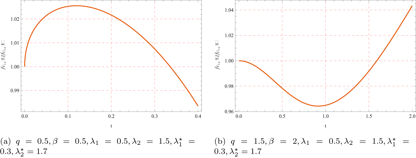


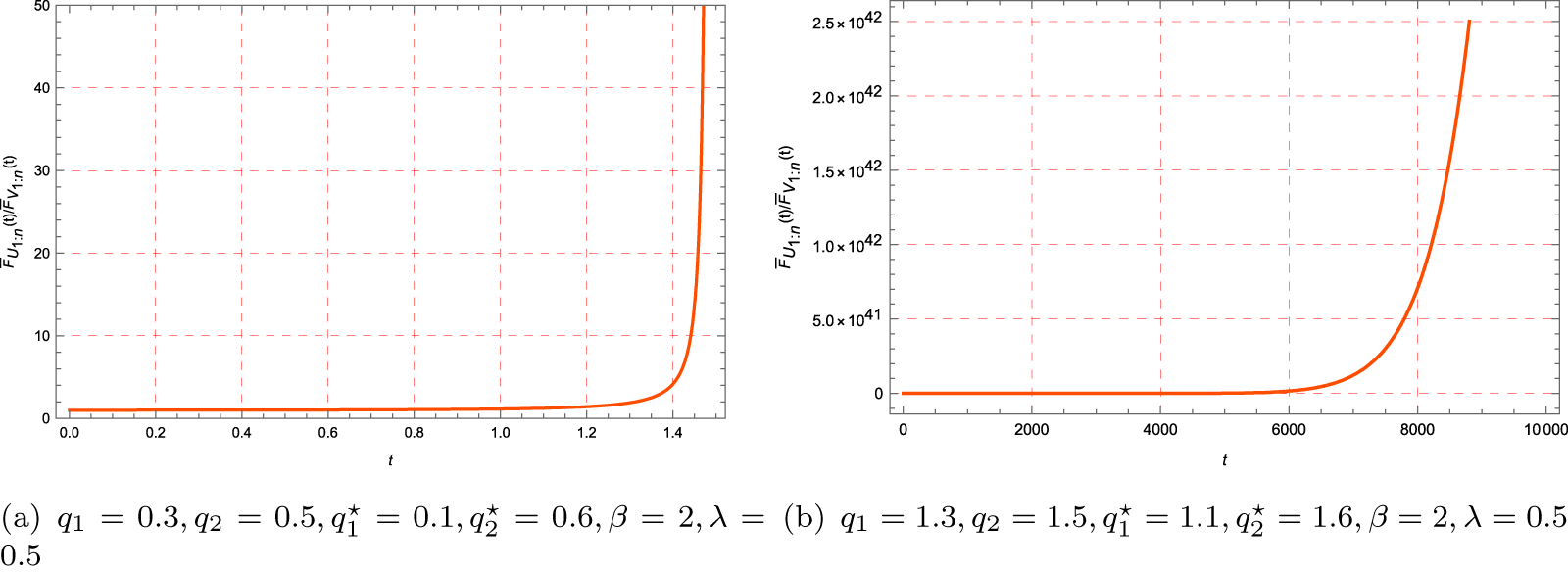


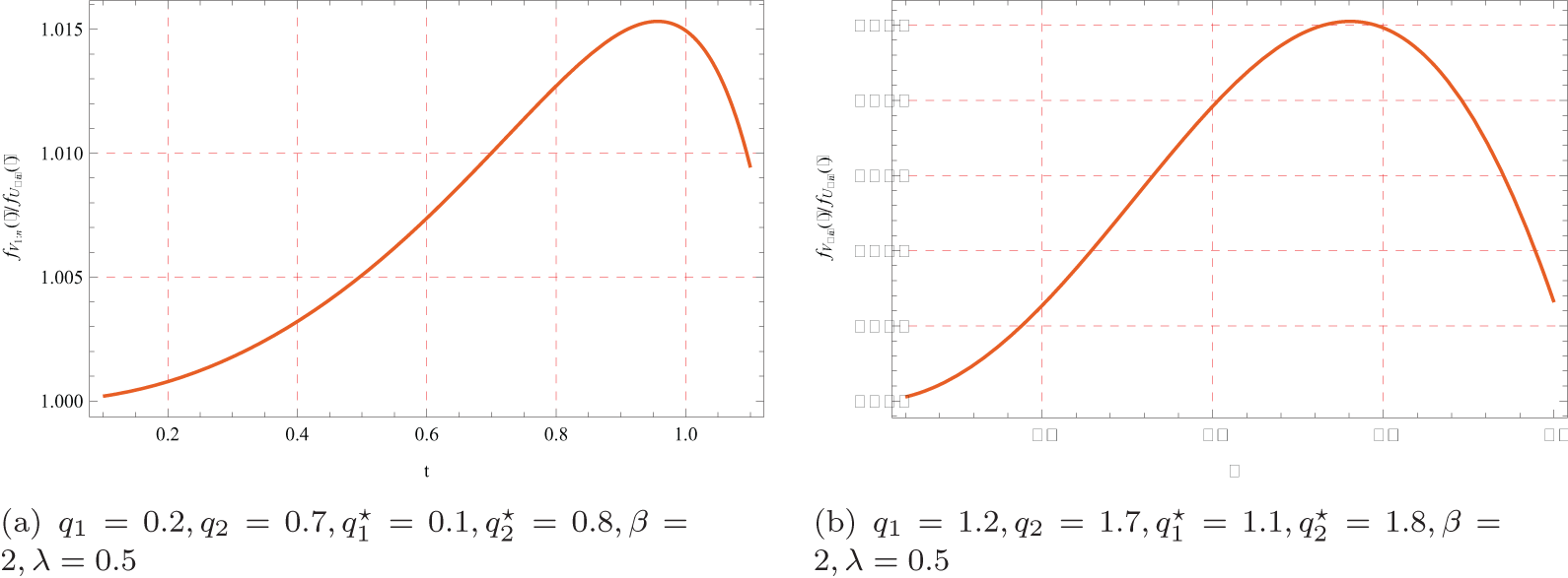


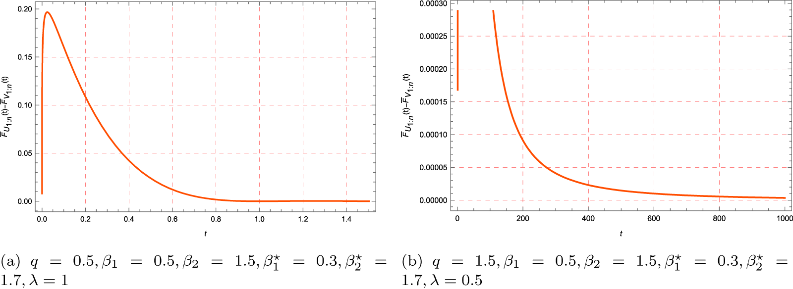


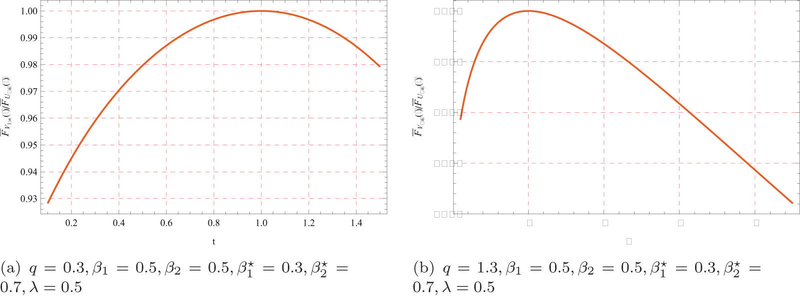


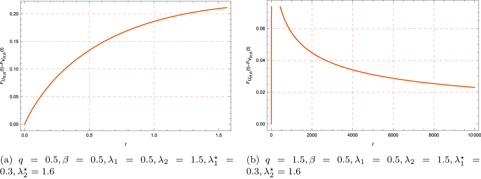


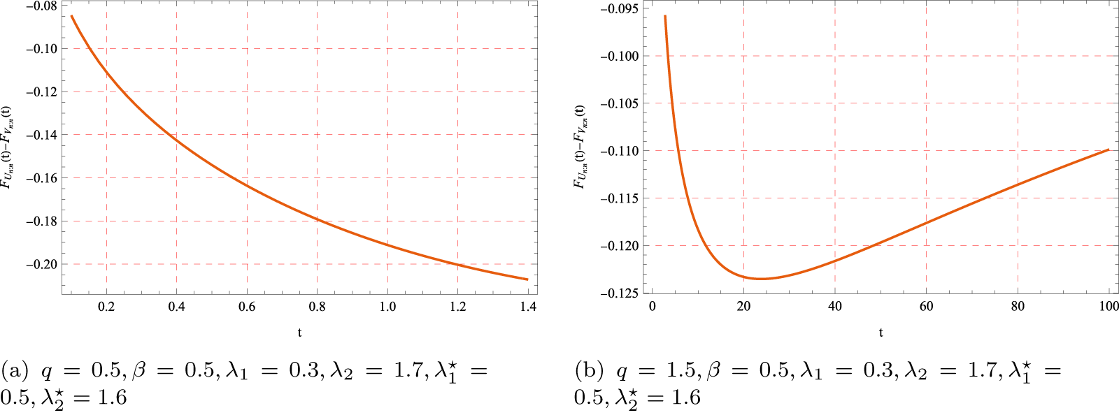


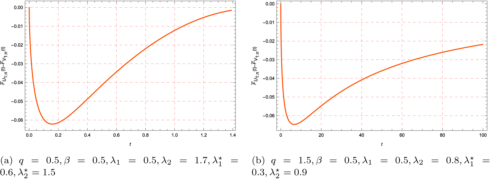


 Open access