


1. Introduction
Inductively coupled plasma (ICP) sources have been a subject of interest in industry and academia for a long time (Hopwood Reference Hopwood1992; Guo et al. Reference Guo, Li, Chang, Han and Lin2022) especially in the field of material and biochemical analysis (Doble et al. Reference Doble, de Vega, Bishop, Hare and Clases2021; Huff Reference Huff2021). An ICP is characterized by high electron density at low pressure, relative simplicity of the device and no need for an additional applied magnetic field. As a low-temperature and high-density plasma source, ICP is beginning to be used in the etching of integrated circuits because of its high etch selectivity for fine etching of large substrates without the tedious steps of wet etching and because the process can be controlled (Smith et al. Reference Smith, Venzor, Newton, Liguori, Gleason, Bornfreund, Johnson, Benson, Stoltz, Varesi, Dinan and Radford2005; Zhang et al. Reference Zhang, Tang, Hu, Yuan, Guan, Li, Cui, Ding, Shi, Xu and Zhuang2021a). Inductively coupled plasma is also widely used for crystal etching (Song et al. Reference Song, Zhang, Liang, Zhao, Min, Shi, Lai and Wang2020), thin-film deposition (Zhang et al. Reference Zhang, Luo, Yu, Li, Wang, Yu, Wang, Hao, Sun, Han, Xiong and Li2021b) and material surface modification (Frye et al. Reference Frye, Donald, Reinhardt, Nikolic, Voss and Harrison2021). Accurate and proficient use of the ICP process requires a clear understanding of the various ICP control factors, such as the gas pressure and absorbed power of the ICP. These control factors can sensitively affect various important physical parameters such as the electron density and electron temperature of the ICP, thus profoundly affecting the accuracy of processes.
At present, there are many methods to measure the electron density and temperature of plasma (Hutchinson Reference Hutchinson2005). The commonly used methods that can measure these two fundamental parameters simultaneously are Langmuir probe (Tichy et al. Reference Tichy, Hubicka, Sicha, Cada, Olejnicek, Churpita, Jastrabik, Virostko, Adamek, Kudrna, Leshkov, Chichina and Kment2009), emission spectroscopy (Akatsuka Reference Akatsuka2019) and Thomson scattering (TS) (Wang et al. Reference Wang, Shi, Li, Feng and Ding2019). Among them, the Langmuir probe method is the most commonly used. This is a method of inferring local plasma parameters by immersing a Langmuir probe in the plasma and measuring the current at various applied voltages (Godyak & Alexandrovich Reference Godyak and Alexandrovich2015). This method has a high spatial resolution. However, it is an interventional measurement because the probe will inevitably interfere with the local measured plasma during the measurement (Bowden et al. Reference Bowden, Kogano, Suetome, Hori, Uchino and Muraoka1999). Optical emission spectroscopy is a non-invasive passive measurement method that does not interfere with the plasma. The plasma parameters are calculated by analysing the intensity and distribution of plasma characteristic spectral lines related to electron density and electron excitation temperature (Akatsuka Reference Akatsuka2019). The experimental set-up is simple, but the spatial resolution is limited due to the chord averaging in the line of sight when solving the plasma parameters. And the calculation of electron temperature is also limited by the premise that the electron excitation temperature is equal to the electron temperature only under the condition of local thermodynamic equilibrium (Kunze Reference Kunze2009). Thomson scattering is a non-invasive active measurement method, which can accurately diagnose a plasma without disturbing the plasma itself. This method can measure plasma parameters in a given region with extremely high spatial–temporal resolution (Carbone et al. Reference Carbone, Sadeghi, Vos, Hubner, van Veldhuizen, van Dijk, Nijdam and Kroesen2015; Tomita et al. Reference Tomita, Sato, Nishikawa, Uchino, Yanagida, Tomuro, Wada, Kunishima, Kodama, Mizoguchi and Sunahara2015) and is not limited by thermodynamic equilibrium (Carbone & Nijdam Reference Carbone and Nijdam2015; Shashurin & Keidar Reference Shashurin and Keidar2015). It is currently recognized as one of the most accurate methods for measuring plasma parameters (Dzierzega, Mendys & Pokrzywka Reference Dzierzega, Mendys and Pokrzywka2014).
In this paper, firstly, the electron density distribution of the plasma generated in an ICP reactor is measured by laser TS experiment, and then the plasma in an ICP reactor of the same size is simulated by building a COMSOL finite element method (FEM) simulation model. The local pressure at the electron density maximum has been calibrated at the same absorbed power. On this basis, the distribution and maximum value of electron density are compared with experimental and simulation data. A comparison of the experimental and simulation results for the electron temperature at the electron density maximum is also presented. This allows a comprehensive comparison between experimental and simulation results of both electron density and electron temperature parameters. Therefore, the validity of ICP FEM simulation is verified comprehensively and effectively for the first time by the state-of-the-art laser TS experiments. This comprehensive verification proves the feasibility of establishing an ICP simulation model using the FEM. This kind of FEM model can be further used to carry out ICP-related process research and improve the process accuracy.
2. The TS experiment
A schematic diagram of the experimental set-up for TS is shown in figure 1. In the red dashed box is the ICP generation system to be studied. A laser beam with a wavelength of 532 nm, a repetition frequency of 30 Hz, a maximum laser pulse energy of 300 mJ and a pulse width of 10 ns is emitted by a Nd:YAG laser. After passing through mirrors 1 to 3, the laser beam enters the ICP cavity through a Brewster quartz window. When passing through the plasma generated by the ICP system, the laser light scattered by electrons, ions and atoms in the plasma is collected by an optical fibre bundle and transmitted to a triple grating spectrometer and intensified CCD (ICCD) camera for imaging or forming a spectrum to complete TS signal detection. Controller DG645 is a time controller that synchronizes the laser pulse with the shutter of the ICCD camera and optimizes the detected signal by changing the exposure time of the ICCD camera. The laser beam passing through the plasma eventually enters the laser stack and terminates its transmission.
Schematic diagram of the TS experiment. In the upper-right corner is a schematic diagram of the optical fibre bundle end face.

To avoid the influence of stray light on the TS signal, Brewster windows are used in the incident and exit windows. To avoid Rayleigh scattering from the air and reflections from other surfaces, the collection end of the optical fibre is placed in a dark chamber. The collection direction of the optical fibre is at an angle of 90° from the laser transmission direction. The detection optical fibre bundle consists of 19 optical fibres arranged linearly along the axis of the ICP. A schematic diagram of the optical fibre bundle end face is shown in the upper-right corner of figure 1. Through a plano-convex lens, the laser–plasma interaction region is demagnified by half and the image is converged on the end of the detection optical fibre bundle. When collecting data, the optical path composed of the plano-convex lens and the optical fibre bundle does not move. The ICP system is driven by two stepper motors to perform axial translation in the x direction and radial translation in the y direction. The TS signals of the measured point are collected simultaneously by nine adjacent fibre channels in the gap of the inductor coil helical antenna, and the final experimental data are obtained by averaging them through data processing software. Each fibre is 200 μm in diameter, giving an axial spatial resolution of 0.4 mm. Affected by the curvature and thickness of the quartz tube, the radial spatial resolution is 2 mm.
When the laser beam is injected into the plasma, the free electrons in the plasma oscillate in the laser electric field. These electrons accelerated by the laser electric field emit electromagnetic radiation, which can be interpreted as scattering of incident laser radiation. The total scattering spectrum of plasma to incident laser consists of three components: TS component generated by free electron scattering; Rayleigh scattering components produced by bound electrons in atoms and ions; and stray light component reflected by the chamber walls and windows. The stray light can be suppressed by a range of methods such as using Brewster windows and special baffles. Compared with the electron cloud around atoms and ions, the free electron velocity is higher, which leads to the Doppler broadening of TS spectral components much wider than that of Rayleigh scattering.
For low-temperature plasmas such as ICP, the total intensity of TS light is proportional to the electron density ne. The total intensity of Rayleigh scattering light is proportional to the density of neutral particles n 0. Therefore, after calibrating the TS results with Rayleigh scattering, ne can be determined from the measured spectra by accurately calibrating the absolute sensitivity of the detection system. When the plasma generator chamber is filled with gas at a given pressure and there is no plasma, the calibration of the intensity of TS light can be completed by measuring the intensity Ig of Rayleigh scattering light.
The Rayleigh scattering light intensity is expressed as (Muraoka, Uchino & Bowden Reference Muraoka, Uchino and Bowden1998)
After the gas is excited in the plasma reactor cavity to generate the plasma, the intensity Ip of the scattering light of the plasma is measured by the same experimental system as
where ${\sigma _{\textrm{Th}}}$ and ${\sigma _R}$
 are the differential cross-sections for TS and Rayleigh scattering (for the calibration gas), respectively. Parameters Δλp and Δλg are the spectral widths of the plasma and gas scattering spectra, respectively, and f sys is a function of the laser energy and the efficiency of the detection system.
Since the same laser and detection system are used for both measurements, f sys is the same in each case, so the electron density is

For a low-temperature plasma such as ICP, the TS spectrum is directly related to the free electron velocity distribution function. When the electron velocity distribution function is a Maxwell function, the TS spectrum is a Gaussian distribution. The electron temperature can be characterized by its half-width, Δλ 1/e (nm), as

Here, λ 0 is the laser wavelength, θ is the scattering angle and k, c and me are the Boltzmann constant, the speed of light and the electron mass respectively.
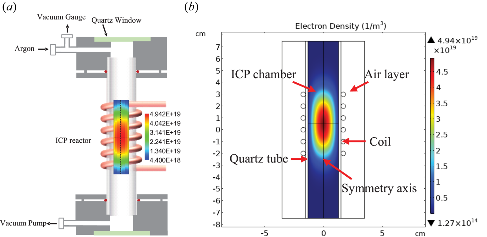
Figure 2(a) shows a schematic diagram of the ICP generator used in the experiment, which is mainly composed of a 15 cm long quartz tube, a six-turn inductor coil, inlet and outlet, etc. The inductor coil is made of hollow copper tube, which is filled with circulating water to take away the heat generated by the plasma in time. The vacuum pump draws out the gas in the chamber from the outlet. During the experiment, the argon to be ionized is slowly released into the chamber from the inlet. A vacuum gauge is placed on the side of the inlet to monitor the pressure in the chamber. When the required pressure is reached, Rayleigh scattering and TS are measured, and the data of electron density and electron temperature are obtained through data processing.
(a) Schematic diagram of ICP generator experimental set-up with experimental results of electron density distribution and (b) FEM simulation results of electron density distribution inside ICP model (gas pressure: 65 Pa; absorbed power: 350 W).
3. The FEM simulation
In this study, COMSOL software is used to model and analyse the ICP. There are seven types of chemical reactions in the chemical process of ICP argon ionization, as shown in table 1.
List of plasma chemical reactions.

According to the types of reactions listed in table 1, reaction 1 is an elastic collision between an electron and an argon atom without energy exchange. However, reactions 2, 4 and 5 need to consume different amounts of electromagnetic energy when they occur. Reaction 2 is an excitation reaction, in which an electron collides with an argon atom and consumes 11.5 eV of energy to excite the argon atom into the metastable state. Reaction 3 is a super-elastic collision, in which an electron collides with a metastable-state argon atom and regains 11.5 eV of energy released by a metastable-state argon atom (Demidov, DeJoseph & Kudryavtsev Reference Demidov, DeJoseph and Kudryavtsev2005; Shen et al. Reference Shen, Wang, Wang, Liu, Liu, Vourlidas, Miao, Ye, Liu and Zhou2012; Liu, Guo & Pu Reference Liu, Guo and Pu2015). At the same time, the metastable-state argon atom returns to a ground-state argon atom after losing energy. Reaction 4 means that an electron consumes 15.8 eV of energy to ionize a ground-state argon atom to release a new electron, and the argon atom becomes an argon ion, which is a typical ionization reaction. Reaction 5 means that an electron only needs 4.24 eV of energy to ionize a metastable argon atom from which a new electron is released, while this metastable argon atom becomes an argon ion. The last column of table 1 shows the maximum reaction rates of the various reactions at 350 W absorbed power and 75 Pa gas pressure. It is evident that the maximum reaction rate of reaction 5 is greater than that of reaction 4 in ionization reactions. Therefore, reaction 5 plays an important role in maintaining the low-pressure argon discharge process (Lymberopoulos & Economou Reference Lymberopoulos and Economou1995; COMSOL 2020). Reactions 6 and 7 respectively indicate that the metastable argon atom is suppressed by another metastable argon atom and ground-state argon atom, returning to a ground-state argon atom and argon ion.
In addition to the bulk reactions, the process also involves two surface reactions (table 2). When metastable argon atoms and argon ions come into contact with the wall, there will be a certain probability (adhesion coefficient) of conversion to ground-state argon atoms.
List of surface reactions.

In conclusion, the FEM generation model of ICP has been established by COMSOL. The inductive coil couples the electromagnetic energy into the argon gas in the tube to cause seven kinds of chemical reactions and two kinds of surface reactions, thus ionizing the argon gas to obtain the plasma. The plasma in the tube is mainly composed of neutral argon atoms, electrons and ions. The electron density ne, electron energy density nɛ and electron temperature Te can be obtained by solving two fluid equations of electron density and electron energy density by FEM. These two fluid equations describe the electron density and the electron energy density as a function of configuration space and time t. The Re is either a source or a sink of electrons which can be described by (COMSOL 2020)
The energy loss or gain due to inelastic collisions, Rε, can be described by

The electron diffusivity ${\boldsymbol{D}_e}$ , energy mobility ${\mu _\varepsilon }$
 and energy diffusivity ${\boldsymbol{D}_\varepsilon }$
 are computed from the electron mobility μe and electron temperature Te using ${\boldsymbol{D}_e} = {\mu _e}{T_e}$
 , ${\mu _\varepsilon } = {\textstyle{5 \over 3}}{\mu _e}$
 and ${\boldsymbol{D}_\varepsilon } = {\mu _\varepsilon }{T_e}$
 . Parameter ${\Gamma _e}$
 is the electron flux and ${\boldsymbol{E}_{\textrm{in}}}$
 is the induced electric field.
According to the specifications of the ICP reactor used during the experiment, the dimensions of the ICP model in COMSOL have been designed. The length of the ICP tube is 15 cm. The inner diameter is 2.6 cm. The wall thickness is 0.2 cm. The inductor coil has six turns, the wire diameter of the coil is 0.4 cm and the turn spacing is 1 cm. During simulation, the temperature parameter is specified as 300 K, the electron transport characteristics are limited to the specified mobility and the electron mobility for isotropic reduction is set to 4 × 1024 (V m s)−1. The thickness of the air layer outside the tube is set to 2 cm. The established FEM simulation model is shown in figure 2(b). An extra-fine mesh is used to fill the triangular mesh with 658 632 elements, and the minimum element is set to 11.2 μm. Boundary layers are created near the tube walls, and each boundary layer is divided into eight sublayers to ensure a smooth transition from the tube wall mesh to the tube inner mesh. Since the plasma ignition time is usually about 1 μs, the maximum ionization state is reached at about 30 μs. To ensure that the plasma reaches a steady state, the transient settings are calculated from 10−6 to 0.1 s.
4. Results and discussion
4.1. Electron density
The spatial distribution of the electron density (Sun et al. Reference Sun, Liu, Zheng, Shi, Li, Zhao, Zhang, Cai, Zhu, Sun, Chao, Yin and Ding2022) can be obtained by ICP FEM simulation. Taking the case of 350 W absorbed power and 65 Pa gas pressure as an example, since the plasma reactor is axisymmetric, the calculated electron density in half of the tube can be mirrored to obtain the simulation results as in figure 2(b). Next, we compare these with the experimental results of electron density distribution in figure 2(a).
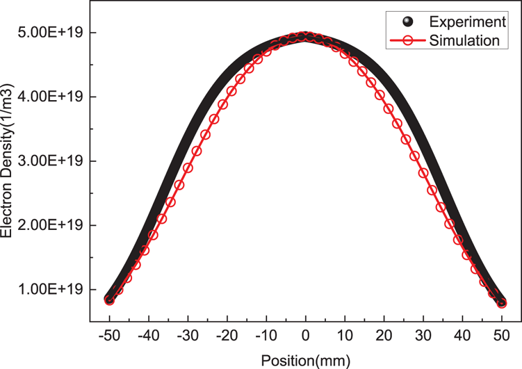
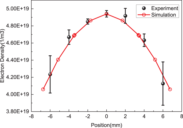
The spatial distributions of electron densities obtained by laser TS experiment and calculated by FEM are cut along the axial and radial directions of the ICP tube at the centre of the tube. The data in both these directions can be compared as shown in figures 3 and 4. The experimental value in the data along the axial direction is slightly larger than the simulated value. The reason is that only a quarter of the ICP tube is measured near the gas outlet in the TS experiment, and the symmetric curve is obtained by mirror processing. In the experiment, the slow flow of gas causes the electrons to drift to the exit zone, which leads to an increase of local electron density. However, the gas in the ICP tube is stationary in the simulation. When the ICP is translated axially driven by a stepper motor, the TS signals of the measured point are collected simultaneously by nine adjacent fibre channels in the gap of the inductor coil helical antenna, and the final experimental data are obtained by averaging them through data processing software. Because the TS signals are blocked by the inductor coil helical antenna, the data cannot be collected continuously. The final axial data are obtained by fitting multiple local continuous data in the gap of the inductor coil helical antenna. The experimental error bars obtained by averaging the axial adjacent points are difficult to display visually in figure 3. Affected by the curvature and thickness of the quartz tube, the spatial resolution of radial points is low. The experimental error bars obtained by averaging radial adjacent points are shown in figure 4.
Comparison of experimental and simulated data of the axial electron density distribution at the centre of the ICP.
Comparison of experimental and simulated data of the radial electron density distribution at the centre of the ICP.
4.2. Electron temperature
The spatial distribution of the plasma density obtained from TS experiment shows that the maximum electron density is in the centre of the ICP tube. Since the low-temperature plasma generated in the ICP reactor has a small spatial distribution gradient of electron temperature, only the central region of the ICP tube has been measured in the experiment. However, the spatial distribution of electron temperature in the tube can be clearly obtained from the FEM simulation results.
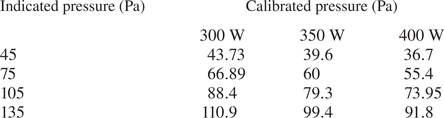
Before comparing the electron temperatures measured by TS experiment with the FEM simulation result at the centre of the ICP tube, the consistency of the plasma absorbed power and the local gas pressure at the centre of the tube should be ensured first. For this purpose, we have conducted the local gas pressure calibration following the method of Sun et al. (Reference Sun, Liu, Zheng, Shi, Li, Zhao, Zhang, Cai, Zhu, Sun, Chao, Yin and Ding2022). In practice, simulations have been carried out for multiple gas pressures under three absorption powers of 300, 350 and 400 W. Local pressure calibrations have been carried out for the four indicated pressures of 45, 75, 105 and 135 Pa under these three different absorbed powers. The calibrated pressures are shown in table 3.
Local pressure calibration table at 300, 350 and 400 W absorbed powers.
Based on the gas pressure calibration, the FEM simulation calculation has been carried out for different gas pressures under 300, 350 and 400 W absorbed powers. Three simulated curves of electron temperature with gas pressure at different absorption power have been obtained and compared with the experimental curves of electron temperature with gas pressure measured by TS, as shown in figure 5. It can be seen from figure 5 that the simulation results of the electron temperature are in reasonable agreement with the experimental results, so the reliability of the FEM ICP model is once again confirmed by the data comparison of the electron temperature. The difference in data comparison may be caused by the inaccuracy of finding the position of the centre of the tube with the maximum electron density measured by the optical fibre bundle in the TS experiment, and it may be caused by the inaccuracy of the gas pressure calibration.
Comparison of experimental and simulation results of the electron temperature curve with gas pressure for (a) 300 W, (b) 350 W and (c) 400 W absorbed power.

5. Conclusions
The spatial distribution and maximum value of electron density in an ICP generator are measured by laser TS experiment, which are in good agreement with the results of FEM simulation (Sun et al. Reference Sun, Liu, Zheng, Shi, Li, Zhao, Zhang, Cai, Zhu, Sun, Chao, Yin and Ding2022). The local pressure at the maximum electron density is calibrated by comparing the experimental and simulated electron densities. On this basis, the electron temperatures measured by TS experiment at the electron density maxima are compared with the FEM simulation results. And the reasonable agreement between them can more fully verify the reliability of the FEM ICP simulation model.
Acknowledgements
Editor Troy Carter thanks the referees for their advice in evaluating this article.
Declaration of interests
The authors report no conflict of interest.


 Open access