


1. Introduction and preliminaries
In this note, we consider the Lipschitz-type domains in the form
 \begin{equation}
\Omega=\{(x,y)\in \mathbb{R}_{+}^{n+1}: y \gt \phi(x) \},
\end{equation}
\begin{equation}
\Omega=\{(x,y)\in \mathbb{R}_{+}^{n+1}: y \gt \phi(x) \},
\end{equation}where  $\phi:{\mathbb R}^n\to \mathbb{R}$ is an $L$-Lipschitz function. On such domains, we would like to study functions satisfying the oscillation condition (*) or the differential inequality (#), to be defined next, and relations between these conditions. Firstly, let us consider a function $u\in C^2(\Omega)$ that satisfies the following oscillation condition on any ball $B_r\subset \Omega$ such that $2B_r\subset \Omega$:
 \begin{equation}
{\rm{osc}}_{B_r}(u)\leq C\,\left(r^{1-n}\,\int_{(1+\eta)B_r}(|\nabla u|^2+|u\Delta u|)\,\mathrm {d} \mathscr{L}^{n+1}\right)^{\frac12}
\end{equation}
\begin{equation}
{\rm{osc}}_{B_r}(u)\leq C\,\left(r^{1-n}\,\int_{(1+\eta)B_r}(|\nabla u|^2+|u\Delta u|)\,\mathrm {d} \mathscr{L}^{n+1}\right)^{\frac12}
\end{equation}for some  $\eta\in [0,1)$ and $C \gt 0$. Such a class has been considered in [Reference González, Koskela, Llorente and Nicolau7], when studying relations between the nontangential maximal function and convenient versions of the area function of general (nonharmonic) functions. A priori, it might not be clear how wide is this family of functions. However, in Section 3.2, we discuss several examples of conditions and functions satisfying (*), in particular, we show in Proposition 3.3 that condition (*) holds if
 \begin{equation*}
u\in C^2\, \hbox{and } |\nabla u|^\alpha\, \hbox{is}\ C\hbox{-quasi-nearly subharmonic, for some } 0 \lt \alpha\leq 2 \ \hbox{and} \ C \gt 0.
\end{equation*}
\begin{equation*}
u\in C^2\, \hbox{and } |\nabla u|^\alpha\, \hbox{is}\ C\hbox{-quasi-nearly subharmonic, for some } 0 \lt \alpha\leq 2 \ \hbox{and} \ C \gt 0.
\end{equation*} The latter condition means that  $|\nabla u|^\alpha$ satisfies the sub-mean value property for all balls in $\Omega$ with some positive constant $C \gt 0$, see (27). In particular, it holds when $|\nabla u|^\alpha$ is subharmonic. This observation allows us to show that solutions of several important semilinear PDEs in the form
 \begin{equation*}
\Delta u= f(u,\nabla u),\quad u\in C^2
\end{equation*}
\begin{equation*}
\Delta u= f(u,\nabla u),\quad u\in C^2
\end{equation*}satisfy condition  $\Delta |\nabla u|^2\geq 0$, see Proposition 3.5.
We consider next the following differential inequality:
 \begin{equation}
|u\Delta u|\le\theta |\nabla u|^2 \ \text{in} \ \Omega
\end{equation}
\begin{equation}
|u\Delta u|\le\theta |\nabla u|^2 \ \text{in} \ \Omega
\end{equation}for some  $\theta \gt 0$. However, further restriction on $\theta$ is necessary in order to control the area function by the non-tangential maximal function of $u$. Namely, we need to assume that $0 \lt \theta \lt 1$. From now on, we will say that a function $u$ satisfies condition (#) if $0 \lt \theta \lt 1$.
The class of functions (#) clearly encloses harmonic ones, but it is wider, see Propositions 3.1 and 3.2. In Section 3.2, we discuss the relations between conditions (#) and (*) and identify the Bloch-type condition, see (29), which for functions satisfying (#) implies (*), see Proposition 3.7 and also Remark 3.6, showing that (#) need not imply (*), in general. Moreover, for the conditions (#) and (*) to hold together, it suffices to assume that
 \begin{align*}
& u\in C^2\, \hbox{satisfies}~(\#)\ \hbox{and } |\nabla u|^\alpha\, \hbox{is}\ C\hbox{-quasi-nearly subharmonic, for some } 0 \lt \alpha\leq 2 \nonumber\\ &\hbox{and } C \gt 0,
\end{align*}
\begin{align*}
& u\in C^2\, \hbox{satisfies}~(\#)\ \hbox{and } |\nabla u|^\alpha\, \hbox{is}\ C\hbox{-quasi-nearly subharmonic, for some } 0 \lt \alpha\leq 2 \nonumber\\ &\hbox{and } C \gt 0,
\end{align*}see the discussion following the statement of Proposition 3.7.
Estimate (*) together with (#) imply that
 \begin{equation}
({\rm{osc}}_{B_r}(u))^2\lesssim_{n,\theta}r^{1-n} \int_{(1+\eta)B_r}|\nabla u|^2\,\mathrm {d} \mathscr{L}^{n+1},
\end{equation}
\begin{equation}
({\rm{osc}}_{B_r}(u))^2\lesssim_{n,\theta}r^{1-n} \int_{(1+\eta)B_r}|\nabla u|^2\,\mathrm {d} \mathscr{L}^{n+1},
\end{equation}which can be understood as the Morrey-type estimate for  $u$.
$u$.
Our main goal is to show the  $\varepsilon$-approximation property for functions satisfying (#) and (*) on domains $\Omega$. The importance of this property comes from an observation that a natural candidate for a Carleson measure of a harmonic function, namely $|\nabla u(x)| \mathrm {d} x$, may fail to be a Carleson measure (see e.g., [Reference Garnett6, Section 6, Ch. VIII]). In order to bypass this problem, the notion of $\varepsilon$-approximability has been introduced [Reference Varopoulos22, Reference Varopoulos23] and has turned out to be important in the studies of the BMO extension problems and Corona theorems [Reference Garnett6, Reference Hofmann and Tapiola13], the characterization of the uniform rectifiability [Reference Hofmann, Le and Morris10–Reference Hofmann, Martell, Mayboroda, Toro and Zhao12] and in the Quantitative Fatou theorems ([Reference Bortz and Hofmann1, Reference Garnett6], see also [Reference Gryszówka8]).
Definition 1.1 ( $\varepsilon$-approximability)

Let  $\varepsilon \gt 0$ and $\Omega\subset \mathbb{R}^{n+1}_{+}$ satisfy (1). We say that a function $u:\Omega\rightarrow\mathbb{R}$ is $\varepsilon$-approximable, if there exists a function $\varphi\in BV_{loc}(\Omega)$ such that
(1)
$\|u-\varphi\|_{\infty} \lt \varepsilon$,(2)
$|\nabla\varphi|\mathrm {d} y$ defines a Carleson measure on
$\Omega$, that is, for every
$x\in\partial\Omega$
(3)\begin{equation}
\sup_{r\in(0,\operatorname{diam} \Omega)}\frac{1}{r^n}\int_{\Omega\cap B(x,r)}|\nabla u(y)|\mathrm {d} \mathscr{L}^{n+1} \leq C_{\varepsilon}.
\end{equation}


The latter condition can be equivalently formulated in terms of the surface measure, since domain  $\Omega$ is given by the Lipschitz graph, and thus the surface measure is $n$-Ahlfors regular on the boundary, implying that $\sigma(B(x,r)\cap \partial \Omega)\approx r^n$. Let us also add that regularity of the $\varepsilon$-approximation $\varphi$ can be improved, see Remark 2.5 at the end of Section 2 below.
Our main goal is to prove the following result.
Theorem 1.1. Let  $\Omega\subset \mathbb{R}^{n+1}_{+}$ be the Lipschitz-graph domain as in (1) and let further $u:\Omega\rightarrow\mathbb{R}$ be bounded and satisfy conditions (#) and (*). Then for every $\varepsilon \gt 0$ function $u$ is $\varepsilon$-approximable in $\Omega$.
The result generalizes the  $\varepsilon$-approximability result for harmonic functions, since the harmonic functions trivially satisfy the condition (#) but also the condition (*), as simple consequence of the subharmonicity of the gradient norm of harmonic functions. Moreover, Theorem 1.1 holds for a wider class of functions, see Section 3 for more details.
In order to give a slightly wider perspective on our results, let us mention that, so far the  $\varepsilon$-approximability has been proven for solutions of elliptic PDEs in the divergence form: ${\rm div}(A\nabla u)=0$, where $|\nabla A|$ satisfies the Carleson measure condition and the growth estimate, see (2.5) and (2.6) in [Reference Bortz and Hofmann1]. Furthermore, it is worth mentioning that in [Reference Hofmann, Martell and Mayboroda11, Remark 5.29] the authors provide some sufficient conditions for the $\varepsilon$-approximability of a function $u$ (not necessarily satisfying any PDE): the boundedness of $u$, the local control of oscillation of $u$ and that it satisfies the Carleson measure estimate in the following form:
 \begin{equation*}
\sup_{x\in\partial\Omega, 0 \lt r \lt \operatorname{diam}(\Omega)}\frac{1}{r^n}\int_{B(x,r)}|\nabla u(y)|^2 \operatorname{dist}(y,\partial \Omega)\mathrm {d} y\le C\|u\|^2_{L^{\infty}(\Omega)}.
\end{equation*}
\begin{equation*}
\sup_{x\in\partial\Omega, 0 \lt r \lt \operatorname{diam}(\Omega)}\frac{1}{r^n}\int_{B(x,r)}|\nabla u(y)|^2 \operatorname{dist}(y,\partial \Omega)\mathrm {d} y\le C\|u\|^2_{L^{\infty}(\Omega)}.
\end{equation*}Notice that, following the spirit of [Reference Hofmann, Martell and Mayboroda11], our condition (*) provides the control of oscillation, whereas our version of the Carleson measure estimate follows from Proposition 2.4 and that is the place where condition (#) is utilized.
We would like to emphasize that for nonnegative subharmonic functions, the condition (#) can be omitted, provided that  $|\nabla u|^\alpha$ is a quasi-nearly subharmonic function for some $\alpha$, as attested by the following observation whose proof we discuss in Section 3.2 and Appendix II.
Theorem 1.2. Let  $u\in C^2$ be nonnegative and subharmonic in an open set $\Omega\subset \mathbb{R}^{n+1}$, that is, $\Delta u\geq 0$. Furthermore, let $|\nabla u|^\alpha$ be a quasi-nearly subharmonic function in $\Omega$ for some $0 \lt \alpha\leq 2$. Then $u$ satisfies (*) and is $\varepsilon$-approximable in domains $\Omega$ as in (1).
The key consequence of Theorems 1.1 and 1.2 is the following Quantitative Fatou Theorem (see Definition 1.3 of the counting function).
Corollary 1.3 (Quantitative Fatou Theorem)
Let  $\Omega\subset \mathbb{R}^{n+1}_{+}$ be the Lipschitz-graph domain as in (1) and let further $u:\Omega\rightarrow\mathbb{R}$ be a bounded $C^2$-function with $\|u\|_{\infty}\le 1$ and satisfy either (i) conditions (#) and (*), or (ii) be a nonnegative subharmonic function for which $|\nabla u|^\alpha$ is a $C$-quasi-nearly subharmonic for some $0 \lt \alpha\leq 2$ and $C \gt 0$. Then for every point $\omega\in\partial\Omega$
 \begin{align*}
\sup_{\substack{0 \lt r \lt r_0}}\frac{1}{r^{n}}\int_{\partial\Omega\cap B(\omega,r)}N(r,\varepsilon,\beta)(z)d\sigma(z)\le C(\varepsilon,\alpha,\beta,n,\Omega),
\end{align*}
\begin{align*}
\sup_{\substack{0 \lt r \lt r_0}}\frac{1}{r^{n}}\int_{\partial\Omega\cap B(\omega,r)}N(r,\varepsilon,\beta)(z)d\sigma(z)\le C(\varepsilon,\alpha,\beta,n,\Omega),
\end{align*}where  $\varepsilon,\alpha,\beta$ are constants in the definition of the counting function $N$. In particular, constant $C$ is independent of $u$.
$u$.
The proof is a verbatim repetition of the proof of Lemma 2.9 in [Reference Kenig, Koch, Pipher and Toro14] and, therefore, we omit it.
Let us remark that the notion of the counting function is known in the literature, see for instance [Reference Bortz and Hofmann1, Reference Garnett6, Reference Kenig, Koch, Pipher and Toro14]. It provides a way to estimate how much a function oscillates while approaching the boundary. The aforementioned works study the counting function in the context of the Quantitative Fatou Property, which generalizes the classical Fatou theorem stating that a non-tangential limit exists at a.e. point of the boundary. In the language of counting function, it reads that the counting function  $N$ is finite a.e.
Preliminaries and notation
Let us recall some necessary definitions and notation used throughout our work.
From now on, unless specified otherwise, by  $\Omega$ we always denote a Lipschitz-type domain as in (1).
Definition 1.2. For  $\alpha \gt 0$, a cone with a vertex at point $(x, \phi(x))\in \partial \Omega$ and aperture $\alpha$ is defined as follows
 \begin{equation*}
\Gamma_{\alpha}(x):=\{(z,y)\in\mathbb{R}^{n+1}_{+}:|z-x| \lt \alpha(y-\phi(x))\}.
\end{equation*}
\begin{equation*}
\Gamma_{\alpha}(x):=\{(z,y)\in\mathbb{R}^{n+1}_{+}:|z-x| \lt \alpha(y-\phi(x))\}.
\end{equation*} Notice that for every  $x\in {\mathbb R}^n$, a cone $\Gamma_{\alpha}(x)$ is congruent to a cone $\{(x,y)\in\mathbb{R}^{n+1}_{+}:|x| \lt \alpha y\}$. However, such cones need not be contained in the domain $\Omega$. Therefore, we introduce the truncated cone:
 \begin{equation*}
\Gamma_{\alpha,s,t}(x):=\Gamma_{\alpha}(x)\cap\{(z,y):\phi(z)+s \lt y \lt \phi(z)+t\},
\end{equation*}
\begin{equation*}
\Gamma_{\alpha,s,t}(x):=\Gamma_{\alpha}(x)\cap\{(z,y):\phi(z)+s \lt y \lt \phi(z)+t\},
\end{equation*}where  $0\le s\le t\le\infty$. In that notation $\Gamma_{\alpha}(x)=\Gamma_{\alpha,0,\infty}(x)$. Since function $\phi$ is $L$-Lipschitz, it holds that $\Gamma_{\alpha,0,t}(x)\subset\Omega$ only for $\alpha \lt \frac{1}{L}$ (and hence, from now on, we only consider $\alpha \lt \frac{1}{L}$).
Definition 1.3 (Counting function)
Let  $\Gamma_{\alpha,0,r}(x)$ be a truncated cone with the vertex at a point $(x, \phi(x)) \in \partial \Omega$. Let $u$ be a continuous function defined on $\Omega$. Fix $\varepsilon \gt 0$, $0 \lt \beta \lt 1$ and $0 \lt r \lt 1$. We say that a sequence of points $x_n\in\Gamma_{\alpha, 0, r}(x)$ is $(r,\varepsilon,\beta,x)$-admissible for $u$ if
 \begin{align*}
|u(x_n)-u(x_{n-1})|\ge\varepsilon\quad\hbox{and}\quad |x_n-x| \lt \beta |x_{n-1}-x|.
\end{align*}
\begin{align*}
|u(x_n)-u(x_{n-1})|\ge\varepsilon\quad\hbox{and}\quad |x_n-x| \lt \beta |x_{n-1}-x|.
\end{align*}Set
 \begin{equation*}
N(r, \varepsilon, \beta)(x):=\sup\{k: \hbox{there exists an } (r, \varepsilon, \beta, x)\hbox{-admissible sequence of length }k\}.
\end{equation*}
\begin{equation*}
N(r, \varepsilon, \beta)(x):=\sup\{k: \hbox{there exists an } (r, \varepsilon, \beta, x)\hbox{-admissible sequence of length }k\}.
\end{equation*} We will call  $N$ a counting function.
Definition 1.4 (Area function)
Let  $f:\Omega\rightarrow[0,\infty]$ be a measurable function. The area function associated with the density $f$ is defined by
 \begin{equation*}
(A_{\alpha}f)(x)=\left(\int_{\Gamma_{\alpha}(x)}f(z,y)(y-\phi(x))^{1-n}\mathrm {d} z\mathrm {d} y\right)^{\frac{1}{2}},\quad x\in {\mathbb R}^n.
\end{equation*}
\begin{equation*}
(A_{\alpha}f)(x)=\left(\int_{\Gamma_{\alpha}(x)}f(z,y)(y-\phi(x))^{1-n}\mathrm {d} z\mathrm {d} y\right)^{\frac{1}{2}},\quad x\in {\mathbb R}^n.
\end{equation*} Similarly, we define the truncated version of the area function  $A_{\alpha,s,t}f$ with respect to cones $\Gamma_{\alpha,s,t}$.
In what follows, we are mostly interested in the case  $f=|\nabla u|^2$ for a function $u\in C^2(\Omega)$. Then we write
 \begin{equation*}
(A_{\alpha,s,t}u)(x):=(A_{\alpha,s,t}|\nabla u|^2)(x)=\left(\int_{\Gamma_{\alpha,s,t}(x)}|\nabla u(z,y)|^2(y-\phi(x))^{1-n}\mathrm {d} z\mathrm {d} y\right)^{\frac{1}{2}}.
\end{equation*}
\begin{equation*}
(A_{\alpha,s,t}u)(x):=(A_{\alpha,s,t}|\nabla u|^2)(x)=\left(\int_{\Gamma_{\alpha,s,t}(x)}|\nabla u(z,y)|^2(y-\phi(x))^{1-n}\mathrm {d} z\mathrm {d} y\right)^{\frac{1}{2}}.
\end{equation*}Definition 1.5 (Nontangential maximal function)
Let  $f:\Omega\rightarrow[0,\infty]$ be a continuous function. The nontangential maximal function of $f$ is defined as follows
 \begin{equation*}
(N_{\alpha}f)(x)=\sup_{\Gamma_{\alpha}(x)}|f(y)|,\quad x\in{\mathbb R}^n.
\end{equation*}
\begin{equation*}
(N_{\alpha}f)(x)=\sup_{\Gamma_{\alpha}(x)}|f(y)|,\quad x\in{\mathbb R}^n.
\end{equation*} As above, the truncated nontangential maximal function of  $f$, denoted by $N_{\alpha,s,t}f$ is defined analogously with respect to cones $\Gamma_{\alpha,s,t}$.
Definition 1.6 (Carleson measure)
Let  $\Omega$ be an open set in $\mathbb{R}^{n+1}$. We say that a (positive) Borel measure $\mu$ on $\Omega$ is a Carleson measure on $\Omega$, if there exists a constant $C \gt 0$ such that
 \begin{equation*}
\mu(\Omega \cap B(x,r))\leq C r^{n},\quad \text{for
all }x \in \partial\Omega \ \text{and }r \gt 0.
\end{equation*}
\begin{equation*}
\mu(\Omega \cap B(x,r))\leq C r^{n},\quad \text{for
all }x \in \partial\Omega \ \text{and }r \gt 0.
\end{equation*} The Carleson measure constant of  $\mu$ is defined as the infimum of constants $C$ above.
Definition 1.7 (Local BV functions)
Let  $\Omega$ be an open set in $\mathbb{R}^{n+1}$. We say that an $L^1_{loc}$-function $f$ has locally bounded variation in $\Omega$, and denote it by $f\in BV_{loc}(\Omega)$, if for any open set $\Omega'\Subset \Omega$ the total variation of $f$ over $\Omega'$ is finite:
 \begin{equation*}
\sup_{\tiny{\Psi\in C_{0}^{1}(\Omega', \mathbb{R}^{n+1}),\,\|\Psi\|_{L^{\infty}}\leq 1}}\int_{\Omega'} f(x)\,{\rm div } \Psi (x)\,\mathrm {d} x \lt \infty.
\end{equation*}
\begin{equation*}
\sup_{\tiny{\Psi\in C_{0}^{1}(\Omega', \mathbb{R}^{n+1}),\,\|\Psi\|_{L^{\infty}}\leq 1}}\int_{\Omega'} f(x)\,{\rm div } \Psi (x)\,\mathrm {d} x \lt \infty.
\end{equation*} Recall that the latter expression defines a (Radon) measure on  $\Omega$, see [Reference Evans and Gariepy3, Section 5.1].
2. Proof of Theorem 1.1
Let us briefly describe our approach to the proof of the main result. Firstly, we recall and formulate some auxiliary notions regarding curved cubes, the associated red and blue sets and the stopping condition allowing us to choose the appropriate families of cubes. Then we a construct function  $\varphi_1$, the first approximation of $\varphi$, see (7) and show in Proposition 2.1 that $\varphi_1$ defines the Carleson measure. The proof of Proposition 2.1 relies on two auxiliary observations, namely Lemmas 2.2 and 2.3. The first one gives a lower bound estimate for the area function and is applied in the proof of Lemma 2.3 to control the sum of volumes of cubes obtained by the stopping procedure. Then, we construct the function $\varphi$, see (20) and show that it $\varepsilon$-approximates the function $u$ in the $L^\infty$-norm. In order to show condition (2) in Definition 1.1, we study the decomposition of the gradient of $\varphi$, see (21), and show that each of its terms leads to the Carleson condition, see estimates (Car1) and (Car2). An important auxiliary result, perhaps of independent interest, is presented in Proposition 2.4 and proved in Appendix I. It gives the $L^2$ bounds for the area function on cubes. The above approach has been inspired by the discussion in [Reference Garnett6, Section 6, Ch. VIII]) and also by [Reference Hofmann, Martell and Mayboroda11].
Let us first set up the stage for the geometric constructions we use to prove our result.
Curved cubes and associated centres. We denote by  $Q_0$ the unit cube in ${\mathbb R}^n$ and by $\{Q_{j_1,\ldots, j_n}^m\}$ the family of dyadic cubes in the dyadic decomposition of $Q_0$:
 \begin{align*}
& Q_{j_1,\ldots, j_n}^m=\{(x_1,\ldots,x_n) \in\mathbb{R}^n: j_i 2^{-m}\le x_i\le (j_i+1)2^{-m}\},\quad \hbox{for } m\in\mathbb{N} \ \hbox{and }\nonumber\\
& j_1,\dots,j_n\in \{0,\ldots, 2^m-1\}.
\end{align*}
\begin{align*}
& Q_{j_1,\ldots, j_n}^m=\{(x_1,\ldots,x_n) \in\mathbb{R}^n: j_i 2^{-m}\le x_i\le (j_i+1)2^{-m}\},\quad \hbox{for } m\in\mathbb{N} \ \hbox{and }\nonumber\\
& j_1,\dots,j_n\in \{0,\ldots, 2^m-1\}.
\end{align*} In the case parameters  $m$ and $j_1,\ldots,j_n$ are fixed or their exact values are not important for the discussion, we will write $Q$ to denote a cube in the $m$-th generation for some $m$. For the sake of notation, in what follows we will usually denote the side length of $Q$ by $l(Q)$ rather than $2^{-m}$.
Let further
 \begin{equation*}
\hat{Q}_0=\{(x,y)\in\mathbb{R}^{n+1}:x\in Q_0, \phi(x)\le y\le 1+\phi(x)\}
\end{equation*}
\begin{equation*}
\hat{Q}_0=\{(x,y)\in\mathbb{R}^{n+1}:x\in Q_0, \phi(x)\le y\le 1+\phi(x)\}
\end{equation*}be an associated curved unit cube in  $\mathbb{R}^{n+1}$, where $\phi :Q_0\rightarrow\mathbb{R}$ is a Lipschitz function. Similarly, for a given cube $Q$, we define the curved cube
 \begin{equation*}
\hat{Q}=\{(x,y)\in\mathbb{R}^{n+1}:x\in Q, \phi(x)\le y\le \phi(x)+l(Q)\}.
\end{equation*}
\begin{equation*}
\hat{Q}=\{(x,y)\in\mathbb{R}^{n+1}:x\in Q, \phi(x)\le y\le \phi(x)+l(Q)\}.
\end{equation*} In what follows, we will often omit the word curved when discussing sets  $\hat{Q}$ and instead simply write cube.
Let  $x_{\hat{Q}}$ denotes a centre of a (curved) cube $\hat{Q}$, that is, $x_{\hat{Q}}:=(x_{Q},\phi(x_Q)+2^{-m-1})$, where $x_Q$ is a centre of $Q$. Note that since by (1) it holds that $\phi$ is $L$-Lipschitz, we have the following inclusions:
 \begin{equation}
B\bigg(x_{\hat{Q}}, \frac{1}{2\sqrt{L^2+1}} l(Q)\bigg) \subset \hat{Q}\subset B\big(x_{\hat{Q}}, C(L)l(Q)\big),\quad C(L):= \frac12\sqrt{L^2+2L+2}.
\end{equation}
\begin{equation}
B\bigg(x_{\hat{Q}}, \frac{1}{2\sqrt{L^2+1}} l(Q)\bigg) \subset \hat{Q}\subset B\big(x_{\hat{Q}}, C(L)l(Q)\big),\quad C(L):= \frac12\sqrt{L^2+2L+2}.
\end{equation} Moreover, we define the associated centre of  $\hat{Q}$ as follows:
 \begin{equation}
x^{l}_{\hat{Q}}=x_{\hat{Q}}+\overline{e_{n+1}}l(Q)=(x_Q,\phi(x_Q)+2^{-m-1}+l(Q))=\left(x_Q,\phi(x_Q)+\frac{3}{2}2^{-m}\right).
\end{equation}
\begin{equation}
x^{l}_{\hat{Q}}=x_{\hat{Q}}+\overline{e_{n+1}}l(Q)=(x_Q,\phi(x_Q)+2^{-m-1}+l(Q))=\left(x_Q,\phi(x_Q)+\frac{3}{2}2^{-m}\right).
\end{equation} The name of this point is justified by the fact that  $x^{l}_{\hat{Q}}$ does not lie inside $\hat{Q}$, and is the centre of the curved cube lying directly above cube $\hat{Q}$ and obtained by shifting up $\hat{Q}$ in $l(Q)$, see Figure 1.
The centre  $x_{\hat{Q}}$ of a cube $\hat{Q}$ and its associated centre $x_{\hat{Q}}^{l}$.

Stopping time conditions. Let us now define a stopping procedure.
Set
 \begin{align*}
G_0&:=\{\hat{Q_0}\} \ \hbox{and denote by } \\
G_1&:=\hbox{a family of maximal curved cubes}\ \hat{Q}\subset\hat{Q_0}\ \hbox{such that }
|u(x_{\hat{Q_0}})-u(x^{l}_{\hat{Q}})| \gt \varepsilon.
\end{align*}
\begin{align*}
G_0&:=\{\hat{Q_0}\} \ \hbox{and denote by } \\
G_1&:=\hbox{a family of maximal curved cubes}\ \hat{Q}\subset\hat{Q_0}\ \hbox{such that }
|u(x_{\hat{Q_0}})-u(x^{l}_{\hat{Q}})| \gt \varepsilon.
\end{align*}Next, define
 \begin{equation*}
G_2=\bigcup_{\hat{Q}\in G_1}G_1(\hat{Q}),
\end{equation*}
\begin{equation*}
G_2=\bigcup_{\hat{Q}\in G_1}G_1(\hat{Q}),
\end{equation*}where  $G_1(\hat{Q})$ is defined the same way as $G_1$ with $\hat{Q_0}$ replaced with $\hat{Q}$. Then define inductively families of sets $G_k$, for $k=2,\ldots$. Denote by $G=\bigcup_{k=0}G_k$. Let us introduce a domain which roughly can be understood as follows: given any curved cube $\hat{Q}\in G$ consider its subset constructed by removing those maximal curved cubes $\hat{Q}_i$, where the jump of the values of $u$ at associated centres is big: $|u(x_{\hat{Q}})-u(x^{l}_{\hat{Q}_i})| \gt \varepsilon$, that is, we define
 \begin{equation*}
R(\hat{Q}):=\hat{Q}\setminus\bigcup_{\hat{Q}_i\in G_1(\hat{Q})}\hat{Q}_i,\quad \hbox{for any }\hat{Q}\in G.
\end{equation*}
\begin{equation*}
R(\hat{Q}):=\hat{Q}\setminus\bigcup_{\hat{Q}_i\in G_1(\hat{Q})}\hat{Q}_i,\quad \hbox{for any }\hat{Q}\in G.
\end{equation*} Thus, set  $R(\hat{Q})$ consists of all curved subcubes in $\hat{Q}$ with small oscillations of $u$, see Figure 3. We remark that this construction is similar to the one in Garnett’s book, see the proof of Theorem 6.1 in [Reference Garnett6, Section 6 in Ch. VIII].
Notice that given two different sets  $\widehat{Q}, \widehat{W}\in G$, the corresponding domains $R(\widehat{Q})$ and $R(\widehat{W})$ can only intersect piecewise along boundaries, but their interiors are pairwise disjoint. Finally, we define blue and red sets, which are essential in our construction. Denote by $T(\hat{Q})$ the set $\hat{Q}$ translated vertically by $\frac{1}{2}l(Q)$:
 \begin{equation}
T(\hat{Q})=\{(x,y)\in\mathbb{R}^{n+1}:x\in Q,\phi(x)+\frac{1}{2}l(Q)\le y\le \phi(x)+\frac{3}{2}l(Q)\}.
\end{equation}
\begin{equation}
T(\hat{Q})=\{(x,y)\in\mathbb{R}^{n+1}:x\in Q,\phi(x)+\frac{1}{2}l(Q)\le y\le \phi(x)+\frac{3}{2}l(Q)\}.
\end{equation} The key feature of sets  $T(\hat{Q})$, to which we appeal several times below, is that they are separated from the graph of the Lipschitz function $\phi$, that is, from the boundary of $\Omega$. Moreover, an important feature of sets $T(\hat{Q})$ is that the associated centre of $\hat{Q}$ is the centre of an upper side of $T(\hat{Q})$, see Figure 2.
The set  $T(\hat{Q})$ (brown set) with respect to the set $\hat{Q}$ (set bounded by black line).

An example of how a set  $R(\hat{Q})$ may look like. Cubes $\hat{Q}_1, \hat{Q}_2, \hat{Q}_3$ are removed from cube $\hat{Q}$ to obtain $R(\hat{Q})$. In general, there may be infinitely many sets that are removed from $\hat{Q}$.

Sets  $T(\hat{Q})$ are not disjoint. However, for a given set $\hat{Q}$, a set $T(\hat{Q})$ intersects only finitely many other sets of the form $T(\hat{Q}_j)$. Moreover, the cardinality of a family of sets $\# \{j: T(\hat{Q})\cap T(\hat{Q}_j)\neq\emptyset\}$ is uniformly bounded for all choices of $\hat{Q}$. When dealing with set $\hat{Q}_0$, we set $T(\hat{Q}_0):=\{(x,y)\in\mathbb{R}^{n+1}:x\in Q_0,\phi(x)+\frac{1}{2}l(Q_0)\le y\le \phi(x)+l(Q_0)\}$, that is, its upper half.
Fix  $\varepsilon \gt 0$ and let $k \gt 0$. We say that $T(\hat{Q})$ is blue, if
 \begin{equation*}
{\rm{osc}}_{T(\hat{Q})}u\le k\varepsilon.
\end{equation*}
\begin{equation*}
{\rm{osc}}_{T(\hat{Q})}u\le k\varepsilon.
\end{equation*} Otherwise, we say that  $T(\hat{Q})$ is red.
Proof of Theorem 1.1
Firstly, we define an auxiliary function  $\varphi_1: \bigcup_{\hat{Q}_k\in G} R(\hat{Q}_k)\to \mathbb{R}$, which later on will be used to define the $\varepsilon$-approximation of $u$, cf. (20)
 \begin{equation}
\varphi_1(z):=\sum_{j=1}^{\infty}\sum_{\hat{Q}_k\in G_j} u(x_{\hat{Q}_k})\chi_{R(\hat{Q}_k)}(z).
\end{equation}
\begin{equation}
\varphi_1(z):=\sum_{j=1}^{\infty}\sum_{\hat{Q}_k\in G_j} u(x_{\hat{Q}_k})\chi_{R(\hat{Q}_k)}(z).
\end{equation} Notice that,  $\varphi_1$ is in fact defined for all $z\in \hat{Q}_0$ and, moreover, for any $\hat{Q} \in G$, it holds that
 \begin{equation}
\int_{\hat{Q}}|\nabla\varphi_1| \,\mathrm {d} \mathscr{L}^{n+1}\le\sum_{\hat{Q}_j\in G} |\hat{Q}\cap\partial R(\hat{Q}_j)|,
\end{equation}
\begin{equation}
\int_{\hat{Q}}|\nabla\varphi_1| \,\mathrm {d} \mathscr{L}^{n+1}\le\sum_{\hat{Q}_j\in G} |\hat{Q}\cap\partial R(\hat{Q}_j)|,
\end{equation}where  $|\cdot|$ denotes the $n$-Hausdorff measure. Here, the expression $|\nabla\varphi_1|$ is understood only in the distributional sense and the component functions of $\nabla\varphi_1$ are the signed measures supported on the appropriate faces in $\partial R(\hat{Q}_j)$, see the discussion for the upper-half space in $\mathbb{R}^2$ on p. 345 in [Reference Garnett6, Section 6, Ch. VIII]. Therefore, $|\chi_{R(\hat{Q}_k)}|$ in (7) are the $n$-Hausdorff measures of $\hat{Q}\cap\partial R(\hat{Q}_j)$ and the above estimate is justified.
Our first step is to prove the following observation, which applied to (8), shows that  $|\nabla\varphi_1| \,\mathrm {d} \mathscr{L}^{n+1}$ is a Carleson measure.
Proposition 2.1. For any  $\hat{Q}$ it holds that $\sum_{\hat{Q}_j\in G}|\hat{Q}\cap\partial R(\hat{Q}_j)|\le C\varepsilon^{-2}l(Q)^n$.
Proof. We may assume, without loss of generality, that  $\hat{Q}\in G$. For otherwise, we consider a family $M(\hat{Q})$ of cubes such that $\hat{Q}_1\in M(\hat{Q})$ if $\hat{Q}_1\subset\hat{Q}$, $\hat{Q}_1\in G$ and $\hat{Q}_1$ is maximal. Then it suffices to prove the assertion for each of the cubes in $M(\hat{Q})$. Hence, from now on, we assume that $\hat{Q}\in G$. In order to show the assertion of Proposition 2.1, we consider two cases depending on whether $\hat{Q}_j$ is contained in $\hat{Q}$ or not and then prove two auxiliary observations in Lemmas 2.2 and 2.3.
Case 1:  $\hat{Q}_j$ is such that $\hat{Q}\cap\partial R(\hat{Q}_j)\neq\emptyset$ and $\hat{Q}_j\not\subset\hat{Q}$.
(1.1) Let
$l(Q_j)\le l(Q)$. Then, it holds that
${\rm int }\hat{Q}\cap {\rm int }\hat{Q}_j=\emptyset$, but the boundaries of curved cubes
$\hat{Q}$ and
$\hat{Q}_j$ still intersect.It holds that
$\hat{Q}\cap\partial R(\hat{Q}_j)$ is a subset of the vertical faces of
$\hat{Q}$ (throughout the paper, by vertical faces we mean those different from the bottom and the top deck of a cube/curved cube). It is the case, since: (1)
$\hat{Q}_j$ has to touch
$\hat{Q}$, as otherwise
$\hat{Q}\cap\partial R(\hat{Q}_j)=\emptyset$ and such a curved cube does not contribute to the sum
$\sum_{\hat{Q}_j\in G}|\hat{Q}\cap\partial R(\hat{Q}_j)|$; (2) since
$l(Q_j)\le l(Q)$, only vertical sides can touch.For different curved cubes
$\hat{Q}_j$ satisfying
$l(Q_j)\le l(Q)$, the corresponding sets
$\hat{Q}\cap\partial R(\hat{Q}_j)$ can intersect along a set of positive
$(n-1)$-Hausdorff measure only, due to the definition of
$G$ and
$R(\hat{Q}_j)$. Indeed, let
$\hat{Q}_l\not=\hat{Q}_k$ be such cubes. Then we have three cases:(a) Cubes
$\hat{Q}_l$ and
$\hat{Q}_k$ have no common face and
${\rm int }\hat{Q}_l \cap {\rm int }\hat{Q}_k=\emptyset$ in which case the corresponding sets
$\hat{Q}\cap\partial R(\hat{Q}_k)$ and
$\hat{Q}\cap\partial R(\hat{Q}_l)$ can intersect along a set of positive
$(n-1)$-Hausdorff measure only. See Figure 4.Figure 4.This figure illustrates (a) and (c) in Case 1.1 in Proposition 2.1. Since (b) may only be observed if the dimension is greater than two, it is not shown as a figure. Red line is a set
$\partial\hat{Q}\cap\partial\hat{Q}_j$. A set
$\partial R(\hat{Q}_j)\cap\hat{Q}$ is a subset of a red set, whereas a set
$\partial R(\hat{Q}_k)\cap\hat{Q}$ is contained in a yellow line above a red one. Therefore, these sets may only intersect along a set of dimension
$n-1$.(b) Cubes
$\hat{Q}_l$ and
$\hat{Q}_k$ have a common face and
${\rm int }\hat{Q}_l \cap {\rm int }\hat{Q}_k=\emptyset$. Then sets
$\hat{Q}\cap\partial R(\hat{Q}_k)$ and
$\hat{Q}\cap\partial R(\hat{Q}_l)$ are subsets of a common face of
$\hat{Q}$, which can only intersect along an
$(n-1)$ dimensional set
$\partial\hat{Q}\cap\partial\hat{Q}_k\cap\partial\hat{Q}_l$.(c) Interiors of cubes
$\hat{Q}_j$ and
$\hat{Q}_k$ intersect, but this means that one of the cubes contains another, for instance, let
$\hat{Q}_j\subset \hat{Q}_k$. However, then
$\hat{Q}_j\cap R(\hat{Q}_k)=\emptyset$ and so the conclusion is as in case (a) above.Therefore, all such
$\hat{Q}_j$ amount to at most
$C(n)l(Q)^n$ in
$\sum_{\hat{Q}_j\in G}|\hat{Q}\cap\partial R(\hat{Q}_j)|$, as they cover at most all vertical faces of
$\hat{Q}$.(1.2) Let
$l(Q_j) \gt l(Q)$.Then, there are at most
$C(n)$ of such cubes
$\hat{Q}_j$. In order to see that this holds, let us consider two cases. If
$\hat{Q}\not\subset\hat{Q}_j$, then there cannot be more of such
$\hat{Q}_j$ than faces of
$\hat{Q}$. This is a consequence of the following observations: (1)
$\hat{Q}\cap\partial R(\hat{Q}_j)\neq\emptyset$ by assumptions, and so
$\hat{Q}$ and
$\hat{Q}_j$ have to touch; (2) since
$\hat{Q}_j\in G$ and
$l(Q_j) \gt l(Q)$, then for each face
$F$ of
$\hat{Q}$ there is at most one curved cube in
$G$ such that it touches
$F$ with the face of side length bigger than
$l(Q)$ and, moreover,
$\hat{Q}\cap\partial R(\hat{Q}_j)\neq\emptyset$ (see also Figure 5).Figure 5.This figure shows Case 1.2 in Proposition 2.1. The purple cube refers to the case
$\hat{Q}\not\subset\hat{Q}_j$ and the green one refers to the case
$\hat{Q}\subset\hat{Q}_j$.Let now
$\hat{Q}\subset\hat{Q}_j$, then there exists exactly one cube in family
$G$ such that
$\hat{Q}\cap\partial R(\hat{Q}_j)\neq\emptyset$. To prove it, note that for any bigger cube
$\hat{Q}_k\in G$ with
$\hat{Q}\subset\hat{Q}_j\subset\hat{Q}_k$ it holds that
$\hat{Q}\cap\partial R(\hat{Q}_k)=\emptyset$, as for such
$\hat{Q}_k$, the cube
$\hat{Q}_j$ is not contained in
$R(\hat{Q}_k)$, as it had to be removed in the construction of
$R(\hat{Q}_k)$. Therefore, there is only one cube such that
$\hat{Q}\subset\hat{Q}_j$ and
$\hat{Q}\cap\partial R(\hat{Q}_j)\neq\emptyset$.Thus, similarly to Case 1.1, such cubes contribute at most
$C(n)l(Q)^n$ to the sum
$\sum_{\hat{Q}_j\in G}|\hat{Q}\cap\partial R(\hat{Q}_j)|$.


In summary, the discussion in Cases 1.1 and 1.2 gives that
 \begin{equation}
\sum_{\hat{Q}_j\in G, \hat{Q}_j\not \subset\hat{Q}}|\hat{Q}\cap\partial R(\hat{Q}_j)|\le C(n)l(Q)^n.
\end{equation}
\begin{equation}
\sum_{\hat{Q}_j\in G, \hat{Q}_j\not \subset\hat{Q}}|\hat{Q}\cap\partial R(\hat{Q}_j)|\le C(n)l(Q)^n.
\end{equation} Case 2:  $\hat{Q}_j$ is such that $\hat{Q}\cap\partial R(\hat{Q}_j)\neq\emptyset$ and $\hat{Q}_j\subset\hat{Q}$.
Then, trivially we have that
 \begin{equation}
\sum_{\hat{Q}_j\in G, \hat{Q}_j\subset\hat{Q}}|\hat{Q}\cap\partial R(\hat{Q}_j)|\le C(n)\sum_{\hat{Q}_j\in G,\hat{Q}_j\subset\hat{Q}}l(Q_j)^n.
\end{equation}
\begin{equation}
\sum_{\hat{Q}_j\in G, \hat{Q}_j\subset\hat{Q}}|\hat{Q}\cap\partial R(\hat{Q}_j)|\le C(n)\sum_{\hat{Q}_j\in G,\hat{Q}_j\subset\hat{Q}}l(Q_j)^n.
\end{equation}To continue the proof of Proposition 2.1, let us prove the following observation.
Lemma 2.2. Let  $\hat{Q}\in G$. It holds that
 \begin{equation*}
\sum_{\hat{Q}_j\in G_1(\hat{Q})}l(Q_j)^n\le C\varepsilon^{-2}\int_{\widetilde{R(\hat{Q})}}|\nabla u(x,y)|^2(y-\phi(x))\,\mathrm {d} x \mathrm {d} y,
\end{equation*}
\begin{equation*}
\sum_{\hat{Q}_j\in G_1(\hat{Q})}l(Q_j)^n\le C\varepsilon^{-2}\int_{\widetilde{R(\hat{Q})}}|\nabla u(x,y)|^2(y-\phi(x))\,\mathrm {d} x \mathrm {d} y,
\end{equation*}where  $C=C(n, L, \theta, \eta)$ and the set $\widetilde{R(\hat{Q})}$ is defined as follows:
 \begin{equation}
\widetilde{R(\hat{Q})}:=\bigcup_{\hat{Q}_j\in G_1(\hat{Q})}\widetilde{\hat{Q_j}}\quad\hbox{where }\quad
\widetilde{\hat{Q_j}}:=
\begin{cases}
T(\hat{Q}_j),\quad \hbox{if } T(\hat{Q}_j) \hbox{is red }\\
\bigcup_{X\in U\hat{Q}_j}\Gamma_{\alpha,0,\frac{1}{2}l(Q_j)}(X),\quad \hbox{if }T(\hat{Q}_j) \hbox{is blue}.
\end{cases}
\end{equation}
\begin{equation}
\widetilde{R(\hat{Q})}:=\bigcup_{\hat{Q}_j\in G_1(\hat{Q})}\widetilde{\hat{Q_j}}\quad\hbox{where }\quad
\widetilde{\hat{Q_j}}:=
\begin{cases}
T(\hat{Q}_j),\quad \hbox{if } T(\hat{Q}_j) \hbox{is red }\\
\bigcup_{X\in U\hat{Q}_j}\Gamma_{\alpha,0,\frac{1}{2}l(Q_j)}(X),\quad \hbox{if }T(\hat{Q}_j) \hbox{is blue}.
\end{cases}
\end{equation} By  $U\hat{Q}_j$, we denote the upper deck of $\hat{Q}_j$. (We refer to the discussion in the proof below, see (17), where the set $\widetilde{R(\hat{Q})}$ is constructed and its meaning explained).
Proof. Let  $\hat{Q}_j\in G_1(\hat{Q})$.
Case 1: The translated curved cube  $T(\hat{Q}_j)$ is red (cf. (6) for the definition of $T(\hat{Q}_j)$). Then, it follows by (2) and (4) that
 \begin{equation}
k^2\varepsilon^2\leq ({\rm{osc}}_{T(\hat{Q}_j)} u)^2\lesssim_{n, L, \theta, \eta} l(Q_j)^{1-n}\int_{T(\hat{Q}_j)}|\nabla u|^2,
\end{equation}
\begin{equation}
k^2\varepsilon^2\leq ({\rm{osc}}_{T(\hat{Q}_j)} u)^2\lesssim_{n, L, \theta, \eta} l(Q_j)^{1-n}\int_{T(\hat{Q}_j)}|\nabla u|^2,
\end{equation}for some  $k \gt 0$ whose exact value will be determined later in this proof. Hence, since $T(\hat{Q}_j)\cap \partial \Omega=\emptyset$ we have that $y-\phi(x)\approx_{n, L} l(Q_j)$ for all $(x,y)\in T(\hat{Q}_j)$. Thus, we get
 \begin{equation}
k^2l(Q_j)^n\lesssim_{n, L, \theta, \eta}\varepsilon^{-2}\int_{T(\hat{Q}_j)}|\nabla u(x,y)|^2(y-\phi(x))\,\mathrm {d} x \mathrm {d} y.
\end{equation}
\begin{equation}
k^2l(Q_j)^n\lesssim_{n, L, \theta, \eta}\varepsilon^{-2}\int_{T(\hat{Q}_j)}|\nabla u(x,y)|^2(y-\phi(x))\,\mathrm {d} x \mathrm {d} y.
\end{equation} Case 2: Set  $T(\hat{Q}_j)$ is blue.
Since  $\hat{Q}_j\in G_1(\hat{Q})$, we know that $|u(x^{l}_{\hat{Q}_j})-u(x_{\hat{Q}})| \gt \varepsilon$. Next, let us define the point
 \begin{equation*}
x^{\frac12 l}_{\hat{Q}_j}:= x^{\hat{Q}_j}+\frac12l(Q_j)\overline{e_{n+1}},
\end{equation*}
\begin{equation*}
x^{\frac12 l}_{\hat{Q}_j}:= x^{\hat{Q}_j}+\frac12l(Q_j)\overline{e_{n+1}},
\end{equation*}which has the same  $x$ coordinate as the centre of the curved cube $x_{\hat{Q}_j}$ but its $y$ coordinate equals $\phi(x)+l(Q_j)$. Thus, one can think that such a point is a vertical projection of the centre of the cube $\hat{Q}_j$ on the upper deck of $\hat{Q}_j$, denoted by $U\hat{Q}_j$. However, notice that $x^{\frac12 l}_{\hat{Q}_j}$ does not lie in the boundary $\partial \Omega$ while we would like to consider a cone with the vertex at that point. Therefore, we let $\Omega_j=\Omega+\overline{e_{n+1}}l(Q_j)$ be a subdomain of $\Omega$ obtained by shifting $\Omega$ vertically up by $l(Q_j)$. Now $x^{\frac12 l}_{\hat{Q}_j} \in\partial\Omega_j$.
Therefore, we have
 \begin{equation}
N_{\alpha,0,\frac{1}{2}l(Q_j)}(u-u(x_{\hat{Q}}))(x^{\frac12 l}_{\hat{Q}_j}) \gt \varepsilon,
\end{equation}
\begin{equation}
N_{\alpha,0,\frac{1}{2}l(Q_j)}(u-u(x_{\hat{Q}}))(x^{\frac12 l}_{\hat{Q}_j}) \gt \varepsilon,
\end{equation}where the (truncated) non-tangential maximal function  $N$ is considered with respect to the domain $\Omega_j$.
We now show that estimate (14) holds not only at  $x^{\frac12 l}_{\hat{Q}_j}$, the centre of the upper deck of $\hat{Q}_j$, but in fact at its all points $X$, that is,
 \begin{equation*}
N_{\alpha,0,\frac{1}{2}l(Q_j)}(u-u(x_{\hat{Q}}))(X) \gt rsim\varepsilon.
\end{equation*}
\begin{equation*}
N_{\alpha,0,\frac{1}{2}l(Q_j)}(u-u(x_{\hat{Q}}))(X) \gt rsim\varepsilon.
\end{equation*} Let us consider vertical shifts of points  $X\in U\hat{Q}_j$ so that they belong to $T(\hat{Q}_j)\setminus \hat{Q}_j$, for example, $X+\tfrac14\overline{e_{n+1}}l(Q_j)$ and notice that they satisfy
 \begin{equation*}
X+\tfrac14\overline{e_{n+1}}l(Q_j) \in\Gamma_{\alpha}(X) \quad\hbox{and }\quad X+\tfrac14\overline{e_{n+1}}l(Q_j) \in T(\hat{Q}_j).
\end{equation*}
\begin{equation*}
X+\tfrac14\overline{e_{n+1}}l(Q_j) \in\Gamma_{\alpha}(X) \quad\hbox{and }\quad X+\tfrac14\overline{e_{n+1}}l(Q_j) \in T(\hat{Q}_j).
\end{equation*} As a consequence we get, by the triangle inequality and since  $T(\hat{Q}_j)$ is blue, that
 \begin{align*}
\varepsilon& \lt |u(x^{l}_{\hat{Q}})-u(x_{\hat{Q}})|\le |u(x^{l}_{\hat{Q}})-u(X+\tfrac14\overline{e_{n+1}}l(Q_j))|+|u(X+\tfrac14\overline{e_{n+1}}l(Q_j))\\
& -u(x_{\hat{Q}})|\le k\varepsilon+|u(X+\tfrac14\overline{e_{n+1}}l(Q_j))-u(x_{\hat{Q}})|
\end{align*}
\begin{align*}
\varepsilon& \lt |u(x^{l}_{\hat{Q}})-u(x_{\hat{Q}})|\le |u(x^{l}_{\hat{Q}})-u(X+\tfrac14\overline{e_{n+1}}l(Q_j))|+|u(X+\tfrac14\overline{e_{n+1}}l(Q_j))\\
& -u(x_{\hat{Q}})|\le k\varepsilon+|u(X+\tfrac14\overline{e_{n+1}}l(Q_j))-u(x_{\hat{Q}})|
\end{align*}and hence
 \begin{equation}
|u(X+\tfrac14\overline{e_{n+1}}l(Q_j))-u(x_{\hat{Q}})| \gt (1-k)\varepsilon.
\end{equation}
\begin{equation}
|u(X+\tfrac14\overline{e_{n+1}}l(Q_j))-u(x_{\hat{Q}})| \gt (1-k)\varepsilon.
\end{equation} Therefore, for every  $X\in U\hat{Q}_j$, we obtain the following estimate
 \begin{equation*}
(1-k)\varepsilon \leq N_{\alpha,0,\frac{1}{2}l(Q_j)}(u-u(x_{\hat{Q}}))(X).
\end{equation*}
\begin{equation*}
(1-k)\varepsilon \leq N_{\alpha,0,\frac{1}{2}l(Q_j)}(u-u(x_{\hat{Q}}))(X).
\end{equation*} Hence, for any  $X\in U\hat{Q}_j$
 \begin{align}(1-k)^2\varepsilon^2 l(Q_j)^n&\lesssim_{n, L} (N_{\alpha,0,\frac{1}{2}l(Q_j)}(u-u(x_{\hat{Q}})))^2(X) \int_{U\hat{Q}_j} \mathrm {d} \mathscr{H}^n \nonumber\\
&\le \int_{U\hat{Q}_j} (N_{\alpha,0,\frac{1}{2}l(Q_j)}(u-u(x_{\hat{Q}})))^2(X)\, \mathrm {d} \mathscr{H}^n\nonumber\\
&\lesssim \int_{U\hat{Q}_j} \int_{\Gamma_{\alpha,0, 1/2 l(Q_j)}(X)} |\nabla u|^2(y-\phi(x)-l(Q_j))^{1-n}\,\mathrm {d} x\mathrm {d} y\,({N\lesssim A})\nonumber\\
&\lesssim \int_{\bigcup \limits_{X\in U\hat{Q}_j}\Gamma_{\alpha,0, 1/2l(Q_j)}(X)}|\nabla u|^2(y-\phi(x)-l(Q_j))\,\mathrm {d} x\mathrm {d} y\nonumber\\
& \qquad\qquad\qquad\qquad\qquad\qquad\qquad\qquad\qquad\qquad (\text{Fubini's Theorem})\nonumber\\
&\le \int_{\bigcup \limits_{X\in U\hat{Q}_j}\Gamma_{\alpha,0, 1/2l(Q_j)}(X)}|\nabla u|^2(y-\phi(x))\,\mathrm {d} x\mathrm {d} y,\end{align}
\begin{align}(1-k)^2\varepsilon^2 l(Q_j)^n&\lesssim_{n, L} (N_{\alpha,0,\frac{1}{2}l(Q_j)}(u-u(x_{\hat{Q}})))^2(X) \int_{U\hat{Q}_j} \mathrm {d} \mathscr{H}^n \nonumber\\
&\le \int_{U\hat{Q}_j} (N_{\alpha,0,\frac{1}{2}l(Q_j)}(u-u(x_{\hat{Q}})))^2(X)\, \mathrm {d} \mathscr{H}^n\nonumber\\
&\lesssim \int_{U\hat{Q}_j} \int_{\Gamma_{\alpha,0, 1/2 l(Q_j)}(X)} |\nabla u|^2(y-\phi(x)-l(Q_j))^{1-n}\,\mathrm {d} x\mathrm {d} y\,({N\lesssim A})\nonumber\\
&\lesssim \int_{\bigcup \limits_{X\in U\hat{Q}_j}\Gamma_{\alpha,0, 1/2l(Q_j)}(X)}|\nabla u|^2(y-\phi(x)-l(Q_j))\,\mathrm {d} x\mathrm {d} y\nonumber\\
& \qquad\qquad\qquad\qquad\qquad\qquad\qquad\qquad\qquad\qquad (\text{Fubini's Theorem})\nonumber\\
&\le \int_{\bigcup \limits_{X\in U\hat{Q}_j}\Gamma_{\alpha,0, 1/2l(Q_j)}(X)}|\nabla u|^2(y-\phi(x))\,\mathrm {d} x\mathrm {d} y,\end{align}where the third ( $N\lesssim A$) inequality follows by the fact that $U\hat{Q}_j\subset \partial \Omega_j$ and by applying the local version of Theorem 1.1 (b) for $p=2$ in [Reference González, Koskela, Llorente and Nicolau7] allowing us to consider the truncated versions of the $N_{\alpha}$ and the $A_{\alpha}$ functions, see the comment following the statement of Theorem 1.2 in [Reference González, Koskela, Llorente and Nicolau7]. Note that in [Reference González, Koskela, Llorente and Nicolau7, Theorem 1.1(b)] its assertion is stated for a variant of the area function, called $S_\alpha$, which is comparable to $A_\alpha$ under the assumption (#).
The set  $\bigcup_{X\in U\hat{Q}_j}\Gamma_{\alpha,0,\frac{1}{2}l(Q_j)}(X)$ consists of the upper-half of $T(\hat{Q}_j)$ and additional parts belonging to neighbouring curved cubes.
However, those parts may only be contained in cubes in the same generation (in the dyadic decomposition) as  $T(\hat{Q}_j)$ and intersect only finitely many of such cubes whose number is estimated by a constant $C(n,\alpha)$. To be more specific, notice that the distance of a point in $\Gamma_{\alpha,0,\frac12l(Q_j)}(X)$ to the axis of the cone can be at most $\frac12\alpha l(Q_j)$. Hence, as we are only interested in cubes in the same generation as $T(\hat{Q}_j)$, in each direction, such a cone can only intersect at most $\lceil\tfrac{\alpha}{2}\rceil$ other cubes. Moreover, as faces of $\hat{Q}_j$ are $n$-dimensional, a cone can overlap with up to $\omega_n(\lceil\frac{\alpha}{2}\rceil)^n$ other cubes, where $\omega_n$ stands for the measure of $n$-dimensional unit ball. Therefore, upon adding up in (16) over all cubes $\hat{Q}_j\in G_1(\hat{Q})$, we increase the constant on the right-hand side only by a factor of $C(n,\alpha)+1$. Thus, the discussion of Case 2 is also completed.
In order to estimate the sum in the assertion of the lemma, we now combine Cases 1 and 2. For this, we also need to analyse how a red set  $T(\hat{Q}_j)$ may intersect other red sets. Notice that the case of cubes in the same generation as a red $T(\hat{Q}_j)$ is already taken care of above. However, it may happen that $T(\hat{Q}_j)$ intersects with sets that belong to one generation below the one of $T(\hat{Q}_j)$, that is, to $(m-1)$-th generation for $T(\hat{Q}_j)$ belonging to the $m$-th generation, for some $m$. Nevertheless, since the number of such cubes is finite, $T(\hat{Q}_j)$ can only intersect $C(n)$ of such cubes.
Finally, we combine estimates (13) and (16) to arrive at the assertion of Lemma 2.2:
 \begin{equation*}
\sum_{\hat{Q}_j\in G_1(\hat{Q})}l(Q_j)^n\le C\varepsilon^{-2}\int_{\widetilde{R(\hat{Q})}}|\nabla u(y)|^2(y-\phi(x)),
\end{equation*}
\begin{equation*}
\sum_{\hat{Q}_j\in G_1(\hat{Q})}l(Q_j)^n\le C\varepsilon^{-2}\int_{\widetilde{R(\hat{Q})}}|\nabla u(y)|^2(y-\phi(x)),
\end{equation*}where  $\widetilde{R(\hat{Q})}:=\bigcup_{\hat{Q}_j\in G_1(\hat{Q})}\widetilde{\hat{Q_j}}$ with
 \begin{equation}
\widetilde{\hat{Q_j}}=
\begin{cases}
T(\hat{Q}_j),\quad \hbox{if } T(\hat{Q}_j) \hbox{is red }\\
\bigcup_{X\in U\hat{Q}_j}\Gamma_{\alpha,0,\frac{1}{2}l(Q_j)}(X),\quad \hbox{if }T(\hat{Q}_j) \ \hbox{is blue}.
\end{cases}
\end{equation}
\begin{equation}
\widetilde{\hat{Q_j}}=
\begin{cases}
T(\hat{Q}_j),\quad \hbox{if } T(\hat{Q}_j) \hbox{is red }\\
\bigcup_{X\in U\hat{Q}_j}\Gamma_{\alpha,0,\frac{1}{2}l(Q_j)}(X),\quad \hbox{if }T(\hat{Q}_j) \ \hbox{is blue}.
\end{cases}
\end{equation} See Figures 6 and 7 illustrating the construction of the set  $\widetilde{R(\hat{Q})}$.
This figure shows how sets  $\widetilde{\hat{Q}_k}$ and $\widetilde{\hat{Q}_j}$ look like for $T(\hat{Q}_k)$ red and $T(\hat{Q}_j)$ blue, respectively. Notice that for a blue $T(\hat{Q_j})$ we drew a bit more of a graph of $\phi$ as a blue set is a union of truncated cones and the way in which the cone is truncated depends on $\phi$.

This figure shows how a domain  $\widetilde{R(\hat{Q})}$ is constructed. It is a union of red and blue sets of the form $\widetilde{\hat{Q}_k}$.

Notice that by (13) and (16), the assertion of the lemma holds with  $C$ depending on $\max\{k^{-2}, (1-k)^{-2}\}$ and, thus taking into account also (15), any $0 \lt k \lt 1$ is suitable.
Lemma 2.2 implies the following observation.
Lemma 2.3. Let  $\hat{Q}\in G$. Then, $\sum_{\hat{Q}_j\in G,\hat{Q}_j\subset\hat{Q}}l(Q_j)^n\le C\varepsilon^{-2}l(Q)^n$.
Before we prove the lemma, let us recall the following notion of shadow of a point and show the claim needed to complete the proof of Lemma 2.3.
Let  $\omega\in\mathbb{R}^n$ and $z\in\Omega$. The shadow of $z$, denoted by ${\rm Sh}(z):={\rm Sh}_{\alpha,s,t}(z)$, is a subset of $\partial\Omega$, defined in the following way:
 \begin{equation*}
(\omega,\phi(\omega))\in {\rm Sh}_{\alpha,s,t}(z)\Leftrightarrow z\in\Gamma_{\alpha,s,t}(\omega).
\end{equation*}
\begin{equation*}
(\omega,\phi(\omega))\in {\rm Sh}_{\alpha,s,t}(z)\Leftrightarrow z\in\Gamma_{\alpha,s,t}(\omega).
\end{equation*}Claim
Let  $z=(x,y)\in C(n,\alpha)\hat{Q}$. Then
 \begin{equation*}
B\Big(\big(x,\phi(x)\big),\frac{\alpha}{1+L\alpha}\big(y-\phi(x)\big)\Big)\cap\partial\Omega\subset {\rm Sh}_{\alpha,0,C(n,\alpha)l(Q)}(z).
\end{equation*}
\begin{equation*}
B\Big(\big(x,\phi(x)\big),\frac{\alpha}{1+L\alpha}\big(y-\phi(x)\big)\Big)\cap\partial\Omega\subset {\rm Sh}_{\alpha,0,C(n,\alpha)l(Q)}(z).
\end{equation*}Proof. Firstly, we may assume that  $z=(0,t)$ and $\phi(0)=0$. Without loss of generality, we can further restrict ourselves to the case when $n=1$. Firstly, we find $\eta\in\mathbb{R}^n$ such that $(\eta,\phi(\eta))\in {\rm Sh}_{\alpha,0,C(n,\alpha)l(Q)}(z)$. Suppose that $\eta \gt 0$. Then, one of the sides of the cone $\Gamma_{\alpha,o,C(n,\alpha)l(Q)}(\eta)$ is given by the equation $y=-\frac{1}{\alpha}x+\frac{1}{\alpha}\eta+\phi(\eta)$.
By the definition of a shadow, point  $(\eta,\phi(\eta))\in {\rm Sh}_{\alpha,0,C(n,\alpha)l(Q)}(z)$ if $z\in\Gamma_{\alpha,o,C(n,\alpha)l(Q)}(\eta)$, which happens if $t \gt \frac{1}{\alpha}\eta+\phi(\eta)$. Therefore, we have $\frac{1}{\alpha}\eta+\phi(\eta) \lt t \lt C(n,\alpha)l(Q)$, and so $\eta \lt -\alpha\phi(\eta)+\alpha C(n,\alpha)l(Q)$. Since $\phi$ is Lipschitz and $\phi(0)=0$, we get $-L\alpha\eta \lt -\alpha\phi(\eta) \lt L\alpha\eta$. Hence, we obtain
 \begin{align*}
\eta \lt -L\alpha\eta+\alpha C(n,\alpha)l(Q),{and \ so }\,\eta \lt \frac{\alpha}{1+L\alpha}C(n,\alpha)l(Q).
\end{align*}
\begin{align*}
\eta \lt -L\alpha\eta+\alpha C(n,\alpha)l(Q),{and \ so }\,\eta \lt \frac{\alpha}{1+L\alpha}C(n,\alpha)l(Q).
\end{align*}
Therefore, for the points  $(\eta,\phi(\eta))$ with $|\eta| \lt \frac{\alpha}{1+L\alpha}C(n,\alpha)l(Q)$ it holds that $(\eta,\phi(\eta))\in {\rm Sh}_{\alpha,0,C(n,\alpha)l(Q)}(z)$.
Moreover, by the definition of a cone, we have  $t \lt C(n,\alpha)l(Q)$. It follows that for $\eta \lt \frac{\alpha}{1+L\alpha}t$, it holds that $\eta\in {\rm S}_{\alpha,0,C(n,\alpha)l(Q)}(z)$. Therefore, $B\big((0,0),\frac{\alpha}{1+L\alpha}t\big)\cap\partial\Omega\subset {\rm Sh}_{\alpha,0,C(n,\alpha)l(Q)}(z)$. Finally, we let $z=(x,y)$ and obtain
 \begin{equation*}
B\big((x,\phi(x)),\frac{\alpha}{1+L\alpha}(y-\phi(x))\big)\cap\partial\Omega\subset {\rm Sh}_{\alpha,0,C(n,\alpha)l(Q)}(z),
\end{equation*}
\begin{equation*}
B\big((x,\phi(x)),\frac{\alpha}{1+L\alpha}(y-\phi(x))\big)\cap\partial\Omega\subset {\rm Sh}_{\alpha,0,C(n,\alpha)l(Q)}(z),
\end{equation*}which concludes the proof of the claim.
Proof of Lemma 2.3
It holds that
 \begin{align*}
\sum_{\hat{Q}_j\in G,\hat{Q}_j\subset\hat{Q}}l(Q_j)^n&=\sum_{k\ge 0}\sum_{\hat{Q}_j\in G_k(\hat{Q})}l(Q_j)^n\\
&=l(Q)^n+\sum_{k\ge 1}\sum_{\hat{Q}_j\in G_k(\hat{Q})}l(Q_j)^n\\
&=l(Q)^n+\sum_{k\ge 1}\,\,\sum_{\hat{Q}^{'}\in G_{k-1}(\hat{Q})}\,\,\sum_{\hat{Q}_j\in G_1(\hat{Q}^{'})}l(Q_j)^n\\
&\lesssim_{n, L, \theta, \eta} l(Q)^n+\varepsilon^{-2}\sum_{k\ge 1}\\
&\sum_{\hat{Q}^{'}\in G_{k-1}(\hat{Q})}\int_{\widetilde{R(\hat{Q}^{'})}}|\nabla u(x,y)|^2(y-\phi(x))\,\mathrm {d} x \mathrm {d} y \,\,\,\,\,(\text{Lemma~2.2})\\
&\lesssim_{n, L, \theta, \eta} l(Q)^n+\varepsilon^{-2}\int_{C(n,\alpha)\hat{Q}}|\nabla u(x,y)|^2(y-\phi(x))\,\mathrm {d} x \mathrm {d} y,\end{align*}
\begin{align*}
\sum_{\hat{Q}_j\in G,\hat{Q}_j\subset\hat{Q}}l(Q_j)^n&=\sum_{k\ge 0}\sum_{\hat{Q}_j\in G_k(\hat{Q})}l(Q_j)^n\\
&=l(Q)^n+\sum_{k\ge 1}\sum_{\hat{Q}_j\in G_k(\hat{Q})}l(Q_j)^n\\
&=l(Q)^n+\sum_{k\ge 1}\,\,\sum_{\hat{Q}^{'}\in G_{k-1}(\hat{Q})}\,\,\sum_{\hat{Q}_j\in G_1(\hat{Q}^{'})}l(Q_j)^n\\
&\lesssim_{n, L, \theta, \eta} l(Q)^n+\varepsilon^{-2}\sum_{k\ge 1}\\
&\sum_{\hat{Q}^{'}\in G_{k-1}(\hat{Q})}\int_{\widetilde{R(\hat{Q}^{'})}}|\nabla u(x,y)|^2(y-\phi(x))\,\mathrm {d} x \mathrm {d} y \,\,\,\,\,(\text{Lemma~2.2})\\
&\lesssim_{n, L, \theta, \eta} l(Q)^n+\varepsilon^{-2}\int_{C(n,\alpha)\hat{Q}}|\nabla u(x,y)|^2(y-\phi(x))\,\mathrm {d} x \mathrm {d} y,\end{align*}where the second inequality follows, by the discussion similar to the one at the end of the proof of Lemma 2.2, from the fact that any cube may be counted at most finitely many times with the uniform constant depending on  $n$ and $\alpha$. However, since sets $\widetilde{R(\hat{Q}^{'})}$ may also contain unions of cones, we may need to consider a cube bigger than $\hat{Q}$ so that $\bigcup \widetilde{R(\hat{Q}^{'})}\subset C(n,\alpha)\hat{Q}$. The proof of Lemma 2.3 will be completed once we show that
 \begin{equation}
\int_{C(n,\alpha)\hat{Q}}|\nabla u(x,y)|^2(y-\phi(x))\,\mathrm {d} x \mathrm {d} y \lesssim_{n, L, \theta, \eta} l(Q)^n.
\end{equation}
\begin{equation}
\int_{C(n,\alpha)\hat{Q}}|\nabla u(x,y)|^2(y-\phi(x))\,\mathrm {d} x \mathrm {d} y \lesssim_{n, L, \theta, \eta} l(Q)^n.
\end{equation} In order to prove this estimate, notice that for  $z=(x,y)\in C(n,\alpha)\hat{Q}$ it holds that $y-\phi(x) \lesssim_{n,L} d(z, \partial \Omega)$. Then the above claim together with the Fubini theorem allow us to obtain the following estimate
 \begin{align}
&\int_{C(n,\alpha)\hat{Q}}|\nabla u(x,y)|^2(y-\phi(x))\,\mathrm {d} x \mathrm {d} y \nonumber \\
&\approx \int_{C(n,\alpha)\hat{Q}}|\nabla u(x,y)|^2 (y-\phi(x))^{1-n} (y-\phi(x))^{n}\,\mathrm {d} x \mathrm {d} y \nonumber\\
&\approx_{n,L, \alpha}\int_{C(n,\alpha)\hat{Q}}|\nabla u(x,y)|^2 (y-\phi(x))^{1-n} \nonumber \\
&\qquad \times \left(\int_{\partial \Omega} \chi_{B((x,\phi(x)), \frac{\alpha}{1+L\alpha}(y-\phi(x))) \cap \partial \Omega}\mathrm {d} \sigma \right)\,\mathrm {d} x \mathrm {d} y \nonumber \\
&\approx_{n,L, \alpha}\int_{C(n,\alpha)\hat{Q}}|\nabla u(x,y)|^2 (y-\phi(x))^{1-n} \left(\int_{\partial \Omega} \chi_{{\rm Sh}_{\alpha, 0, C(n,\alpha)l(Q)}}\mathrm {d} \sigma \right) \,\mathrm {d} x \mathrm {d} y \nonumber \\
&\approx_{n,L, \alpha}\int_{\partial \Omega} \left(\int_{C(n,\alpha)\hat{Q}}|\nabla u(x,y)|^2 (y-\phi(x))^{1-n} \chi_{\Gamma_{\alpha, 0, C(n,\alpha)l(Q)}} \,\mathrm {d} x \mathrm {d} y\right)\, \mathrm {d} \sigma \nonumber \\
&\qquad\qquad\qquad\qquad\qquad\qquad\qquad\qquad\qquad\qquad\qquad\qquad\qquad\,\,\,(\text{Fubini's theorem})\nonumber \\
&\approx_{n,L, \alpha}\int_{Q} \left(A_{\alpha, 0, C(n,\alpha)l(Q)} u\right)^2(x)\,\mathrm {d} x
\lesssim (C(n,\alpha)l(Q))^n.
\end{align}
\begin{align}
&\int_{C(n,\alpha)\hat{Q}}|\nabla u(x,y)|^2(y-\phi(x))\,\mathrm {d} x \mathrm {d} y \nonumber \\
&\approx \int_{C(n,\alpha)\hat{Q}}|\nabla u(x,y)|^2 (y-\phi(x))^{1-n} (y-\phi(x))^{n}\,\mathrm {d} x \mathrm {d} y \nonumber\\
&\approx_{n,L, \alpha}\int_{C(n,\alpha)\hat{Q}}|\nabla u(x,y)|^2 (y-\phi(x))^{1-n} \nonumber \\
&\qquad \times \left(\int_{\partial \Omega} \chi_{B((x,\phi(x)), \frac{\alpha}{1+L\alpha}(y-\phi(x))) \cap \partial \Omega}\mathrm {d} \sigma \right)\,\mathrm {d} x \mathrm {d} y \nonumber \\
&\approx_{n,L, \alpha}\int_{C(n,\alpha)\hat{Q}}|\nabla u(x,y)|^2 (y-\phi(x))^{1-n} \left(\int_{\partial \Omega} \chi_{{\rm Sh}_{\alpha, 0, C(n,\alpha)l(Q)}}\mathrm {d} \sigma \right) \,\mathrm {d} x \mathrm {d} y \nonumber \\
&\approx_{n,L, \alpha}\int_{\partial \Omega} \left(\int_{C(n,\alpha)\hat{Q}}|\nabla u(x,y)|^2 (y-\phi(x))^{1-n} \chi_{\Gamma_{\alpha, 0, C(n,\alpha)l(Q)}} \,\mathrm {d} x \mathrm {d} y\right)\, \mathrm {d} \sigma \nonumber \\
&\qquad\qquad\qquad\qquad\qquad\qquad\qquad\qquad\qquad\qquad\qquad\qquad\qquad\,\,\,(\text{Fubini's theorem})\nonumber \\
&\approx_{n,L, \alpha}\int_{Q} \left(A_{\alpha, 0, C(n,\alpha)l(Q)} u\right)^2(x)\,\mathrm {d} x
\lesssim (C(n,\alpha)l(Q))^n.
\end{align}The last inequality follows from the following observation, whose proof we present in the appendix.
Proposition 2.4. Let  $\Omega\subset \mathbb{R}^{n+1}_{+}$ be the Lipschitz-graph domain as in (1) and let further $u:\Omega\rightarrow\mathbb{R}$ be bounded and satisfy condition (#). Then for any dyadic cube $Q\subset {\mathbb R}^n$ it holds that
 \begin{equation*}
\int_{Q} \left(A_{\alpha, 0, l(Q)} u\right)^2(x)\,\mathrm {d} x \lt c (l(Q))^n,
\end{equation*}
\begin{equation*}
\int_{Q} \left(A_{\alpha, 0, l(Q)} u\right)^2(x)\,\mathrm {d} x \lt c (l(Q))^n,
\end{equation*}where the constant  $c$ depends only on $\alpha$, $\theta$ as in (#), $n$ and the Lipschitz constant $L$ of $\phi$.
Therefore, the inequality (18) is proven and, hence, the proof of Lemma 2.3 is completed.
Upon combining the discussion in (9) and (10) together with Lemma 2.3, we complete the proof of Proposition 2.1.
Continuation of the proof of Theorem 1.1:
Recall that, as already mentioned in the discussion following (7) and (8), Proposition 2.1 shows that  $|\nabla\varphi_1| \mathrm {d} \mathscr{L}^{n+1}$ is a Carleson measure in $\Omega$. Let us now define the following function $\varphi:\Omega\to\mathbb{R}$:
 \begin{equation}
\varphi(z)=
\begin{cases}
u(z) &{if}\ z\ \hbox{belongs to any red } T(\hat{Q})\\
\varphi_1(z) & \hbox{otherwise}
\end{cases}
\end{equation}
\begin{equation}
\varphi(z)=
\begin{cases}
u(z) &{if}\ z\ \hbox{belongs to any red } T(\hat{Q})\\
\varphi_1(z) & \hbox{otherwise}
\end{cases}
\end{equation} Our goal is to prove that  $\varphi$ is an $\varepsilon$-approximation of $u$ as in Definition 1.1. Denote by
 \begin{align*}
& {\small RED} \ \text{the union of all red sets} \ T(\hat{Q}) \ \text{and by} \ {\small BLUE} \ \text{the union of all blue sets} \\
&\quad T(\hat{Q}), \text{for} \ \hat{Q}\subset \hat{Q_0}.
\end{align*}
\begin{align*}
& {\small RED} \ \text{the union of all red sets} \ T(\hat{Q}) \ \text{and by} \ {\small BLUE} \ \text{the union of all blue sets} \\
&\quad T(\hat{Q}), \text{for} \ \hat{Q}\subset \hat{Q_0}.
\end{align*} If  $z\in{\small RED}$, then $u(z)-\varphi(z)=0$, whereas if $z\in{\small BLUE}$, then $z\in R(\hat{Q})$ for some $\hat{Q}\in G$. Suppose that $z\in T(\hat{Q}_1)$. Since, by the definition (6), the set $T(\hat{Q}_1)$ is a vertical translation of cube $\hat{Q}_1$, its upper half may be a subset of one $R$-set (i.e., $R(\hat{Q})$ for some $\hat{Q}\in G$), while its lower half may lie in another $R$-set. Moreover, it can also happen that $T(\hat{Q}_1)$ is entirely contained in one $R$-set. This discussion leads to the following two cases.
If  $T(\hat{Q}_1)\subset R(\hat{Q})$, then
 \begin{align*}
|u(z)-\varphi(z)|&=|u(z)-\varphi_1(z)| \\
&=|u(z)-u(x_{\hat{Q}_1})\chi_{R(\hat{Q})}(z)| \le |u(z)-u(x^{l}_{\hat{Q}_1})|+ \\
&\quad |u(x^{l}_{\hat{Q}_1})-u(x_{\hat{Q}})|\le k\varepsilon + \varepsilon,
\end{align*}
\begin{align*}
|u(z)-\varphi(z)|&=|u(z)-\varphi_1(z)| \\
&=|u(z)-u(x_{\hat{Q}_1})\chi_{R(\hat{Q})}(z)| \le |u(z)-u(x^{l}_{\hat{Q}_1})|+ \\
&\quad |u(x^{l}_{\hat{Q}_1})-u(x_{\hat{Q}})|\le k\varepsilon + \varepsilon,
\end{align*}where the first  $k\varepsilon$ comes from the fact that $T(\hat{Q}_1)$ is blue and the second $\varepsilon$ is obtained because $\hat{Q}_1$ is not entirely removed from $R(\hat{Q})$.
If  $T(\hat{Q}_1)\not\subset R(\hat{Q})$, then suppose first that $z$ belongs to the lower half of $T(\hat{Q}_1)$, that is, $z\in T(\hat{Q}_1)\cap \hat{Q}_1$. Then $z\in R(\hat{Q}_1)$ and since $T(\hat{Q}_1)$ is blue, we have that $|u(z)-\varphi(z)|\le k\varepsilon$.
If  $z$ belongs to the upper half of $T(\hat{Q}_1)$, that is, $z\in T(\hat{Q}_1)\setminus \hat{Q}_1$, then $z$ lies in $T(P\hat{Q}_1)$, where $P\hat{Q}_1$ denotes the parent of $\hat{Q}_1$, meaning the smallest cube $\hat{Q}$ containing $\hat{Q}_1$. Moreover, $z\in T(P\hat{Q}_1)\cap P\hat{Q}_1$. If $T(P\hat{Q}_1)$ is blue, then $|u(z)-\varphi(z)|\le k\varepsilon$ in a similar manner as before. Otherwise, if $T(P\hat{Q}_1)$ is red, then this case has already been taken care of above (see also Figure 8).
This figure shows the situation when  $z$ belongs to the upper half of $T(\hat{Q}_1)$. A green cube is a cube $\hat{Q}_1$, the cube bounded by a brown line is a parent of $\hat{Q}_1$, that is, $P\hat{Q}_1$.

This discussion shows that  $\|u-\varphi\|_{\infty}\le (k+1)\varepsilon$.
Notice that
 \begin{equation}
\nabla\varphi = (\nabla\varphi_1)\chi_{\hat{Q}_0\setminus{\small RED}}+(\nabla u)\chi_{\small RED}+J,
\end{equation}
\begin{equation}
\nabla\varphi = (\nabla\varphi_1)\chi_{\hat{Q}_0\setminus{\small RED}}+(\nabla u)\chi_{\small RED}+J,
\end{equation}where  $J$ denotes jumps along boundaries of Red. We already proved that $|\nabla\varphi_1|\mathrm {d} \mathscr{L}^{n+1}$ is a Carleson measure. Therefore, by the definition of $\varphi$ in (20), it remains to prove that on the set Red, the measure $|\nabla \varphi|\mathrm {d} \mathscr{L}^{n+1}=|\nabla u|\mathrm {d} \mathscr{L}^{n+1}$ is a Carleson measure and that also $J$ gives a Carleson measure. Since $\|u\|_{\infty}\le 1$ and $\|u-\varphi\|_{\infty}\lesssim_k\varepsilon$ it follows that $|J|\lesssim (1+\varepsilon)\sum_{T(\hat{Q}_j) {red}}l(Q_j)^n$. From those, it will follow that $|\nabla\varphi|$ defines a Carleson measure.
Our goal amounts to proving the two inequalities (Car1) and (Car2). The first one allows us to handle the  $\nabla u$ term in (21), while (Car2) takes care of the $J$ part.
 \begin{equation}
\quad \sum_{T(\hat{Q}_j) {red},\, \hat{Q}_j\subset \hat{Q} } \int_{T(\hat{Q}_j)}|\nabla u|\lesssim_{n, L, \eta} \frac{1}{\varepsilon} l(Q)^n,
\end{equation}
\begin{equation}
\quad \sum_{T(\hat{Q}_j) {red},\, \hat{Q}_j\subset \hat{Q} } \int_{T(\hat{Q}_j)}|\nabla u|\lesssim_{n, L, \eta} \frac{1}{\varepsilon} l(Q)^n,
\end{equation} \begin{equation}\quad \sum_{T(\hat{Q}_j) {red},\, \hat{Q}_j\subset \hat{Q} } l(Q_j)^n\lesssim_{n, L, \eta} \frac{1}{\varepsilon^2} l(Q)^n.
\end{equation}
\begin{equation}\quad \sum_{T(\hat{Q}_j) {red},\, \hat{Q}_j\subset \hat{Q} } l(Q_j)^n\lesssim_{n, L, \eta} \frac{1}{\varepsilon^2} l(Q)^n.
\end{equation} Let us begin with proving (Car2). Let us choose a finite cover by hyperbolic balls centred at points of any given cube  $T(\hat{Q}_j)$. Since we are interested now in red cubes, we have by (2) that for any such ball $B_r$ of radius $r$ from the covering of $T(\hat{Q}_j)$ it holds
 \begin{equation}
\varepsilon^2\le ({\rm{osc}}_{B_r} u)^2\lesssim r^{1-n}\int_{(1+\eta)B_r} |\nabla u|^2,\quad\hbox{for some fixed }\eta\in [0,1).
\end{equation}
\begin{equation}
\varepsilon^2\le ({\rm{osc}}_{B_r} u)^2\lesssim r^{1-n}\int_{(1+\eta)B_r} |\nabla u|^2,\quad\hbox{for some fixed }\eta\in [0,1).
\end{equation} Notice that for any point  $z\in T(\hat{Q}_j)$ it holds that the distance $\delta_j (z)$ of $z$ to the bottom face of $\hat{Q}_j$, satisfies $\frac12 l(Q_j)\leq \delta_j (z) \leq l(Q_j)$. Moreover, for any hyperbolic ball $B_r$ containing $z$ it holds that $r\leq \delta_j (z) \leq Cr$, for some fixed numerical constant $C \gt 0$. Thus, we have that
 \begin{equation*}
r\approx \delta_j (z) \approx l(Q_j).
\end{equation*}
\begin{equation*}
r\approx \delta_j (z) \approx l(Q_j).
\end{equation*} Let us fix one ball  $B_r$ from the covering of $T(\hat{Q}_j)$, centred at the point $x_{\hat{Q}_j}+\overline{e_{n+1}}\frac12l(Q_j)$ a centre of $T(\hat{Q}_j)$ and such that $(1+\eta)B_r\Subset T(\hat{Q}_j)$. Such a ball can be obtained by similar reasoning as in (4) and $r:=\frac{l(Q_j)}{(1+\eta)(C(L)+1)^4}$ would suffice.
Therefore, upon multiplying inequality (22) by  $l(Q_j)^n$, we get
 \begin{equation}
l(Q_j)^n\le \frac{1}{\varepsilon^2}\int_{T(\hat{Q}_j)}|\nabla u|^2 \delta_j(z),
\end{equation}
\begin{equation}
l(Q_j)^n\le \frac{1}{\varepsilon^2}\int_{T(\hat{Q}_j)}|\nabla u|^2 \delta_j(z),
\end{equation}as the above constructed ball  $B_r$ satisfies $(1+\eta)B_r\subset T(\hat{Q}_j)$. From this and the Hölder inequality together with (4), we infer the following estimate
 \begin{align*}
\left(\int_{T(\hat{Q}_j)}|\nabla u|\right)^2 & \lesssim_{n,L} \left(\int_{T(\hat{Q}_j)}|\nabla u|^2\right)l(Q_j)^{n+1}\approx \nonumber\\
&\left(\int_{T(\hat{Q}_j)}|\nabla u|^2 \delta_j\right)l(Q_j)^n
\lesssim \frac{1}{\varepsilon^2}\left(\int_{T(\hat{Q}_j)}|\nabla u|^2 \delta_j\right)^2,
\end{align*}
\begin{align*}
\left(\int_{T(\hat{Q}_j)}|\nabla u|\right)^2 & \lesssim_{n,L} \left(\int_{T(\hat{Q}_j)}|\nabla u|^2\right)l(Q_j)^{n+1}\approx \nonumber\\
&\left(\int_{T(\hat{Q}_j)}|\nabla u|^2 \delta_j\right)l(Q_j)^n
\lesssim \frac{1}{\varepsilon^2}\left(\int_{T(\hat{Q}_j)}|\nabla u|^2 \delta_j\right)^2,
\end{align*}which gives
 \begin{equation*}
\int_{T(\hat{Q}_j)}|\nabla u|\lesssim_{n, L} \frac{1}{\varepsilon}\int_{T(\hat{Q}_j)}|\nabla u|^2 \delta_j.
\end{equation*}
\begin{equation*}
\int_{T(\hat{Q}_j)}|\nabla u|\lesssim_{n, L} \frac{1}{\varepsilon}\int_{T(\hat{Q}_j)}|\nabla u|^2 \delta_j.
\end{equation*}We now proceed with the first inequality (Car1), as it turns out that proving it will also complete the proof of (Car2).
 \begin{align}
\sum_{T(\hat{Q}_j) {red},\,\hat{Q}_j\subset \hat{Q} } \int_{T(\hat{Q}_j)}|\nabla u(z)| &\lesssim \sum_{T(\hat{Q}_j) {red},\,\hat{Q}_j\subset \hat{Q} }\frac{1}{\varepsilon}\int_{T(\hat{Q}_j)}|\nabla u(z)|^2 \delta_j(z) \nonumber\\
&\lesssim_{n,L} \frac{1}{\varepsilon}\int_{\hat{Q}}|\nabla u(z)|^2 \delta(z),
\end{align}
\begin{align}
\sum_{T(\hat{Q}_j) {red},\,\hat{Q}_j\subset \hat{Q} } \int_{T(\hat{Q}_j)}|\nabla u(z)| &\lesssim \sum_{T(\hat{Q}_j) {red},\,\hat{Q}_j\subset \hat{Q} }\frac{1}{\varepsilon}\int_{T(\hat{Q}_j)}|\nabla u(z)|^2 \delta_j(z) \nonumber\\
&\lesssim_{n,L} \frac{1}{\varepsilon}\int_{\hat{Q}}|\nabla u(z)|^2 \delta(z),
\end{align}where in the last inequality, by  $\delta(z)$ we denote the distance of point $z$ to the bottom face of $\hat{Q}$. Moreover, the last inequality holds true, due to the observation that although sets $T(\hat{Q}_j)$ may, in general intersect, for different $\hat{Q}_j$, each point in $\hat{Q}$ belongs to at most two sets $T(\hat{Q}_j)$. Thus, the integral on the right-hand side of the last estimate in (24) may increase at most twice. Finally, similarly to the discussion of estimate (18) in the proof of Lemma 2.3, we observe that for any point $\omega\in \hat{Q}\cap \partial \Omega$, that is, in the bottom face of cube $\hat{Q}$, it holds that
 \begin{align*}
z= & (x,y)\in \Gamma_{\alpha, 0, l(Q)}(\omega)\,\Leftrightarrow \nonumber\\
& (\omega,\phi(\omega)) \in {\rm Sh}_{\alpha,0,l(Q)}(z)\supset B\Big((x,\phi(x)),\frac{\alpha}{1+L\alpha}(y-\phi(x))\Big) \cap \partial \Omega.
\end{align*}
\begin{align*}
z= & (x,y)\in \Gamma_{\alpha, 0, l(Q)}(\omega)\,\Leftrightarrow \nonumber\\
& (\omega,\phi(\omega)) \in {\rm Sh}_{\alpha,0,l(Q)}(z)\supset B\Big((x,\phi(x)),\frac{\alpha}{1+L\alpha}(y-\phi(x))\Big) \cap \partial \Omega.
\end{align*} Moreover, notice that for  $z=(x,y)\in \hat{Q}$ it holds that $\delta(z) \leq l(Q) \approx_{n,L} y-\phi(x)$. These observations, together with the analogous computations as in (19) and Proposition 2.4, imply that
 \begin{align}\frac{1}{\varepsilon}\int_{\hat{Q}}|\nabla u(z)|^2 \delta(z)\,\mathrm {d} z &\approx_{n,L}
\frac{1}{\varepsilon}\int_{\hat{Q}}|\nabla u(x,y)|^2 (y-\phi(x))^{1-n} (y-\phi(x))^{n}\,\mathrm {d} x \mathrm {d} y \nonumber \\
&\approx_{n,L, \alpha} \frac{1}{\varepsilon} \int_{Q} \left(A_{\alpha, 0, l(Q)} u\right)^2(x)\,\mathrm {d} x
\lesssim \frac{1}{\varepsilon}(l(Q))^n.\end{align}
\begin{align}\frac{1}{\varepsilon}\int_{\hat{Q}}|\nabla u(z)|^2 \delta(z)\,\mathrm {d} z &\approx_{n,L}
\frac{1}{\varepsilon}\int_{\hat{Q}}|\nabla u(x,y)|^2 (y-\phi(x))^{1-n} (y-\phi(x))^{n}\,\mathrm {d} x \mathrm {d} y \nonumber \\
&\approx_{n,L, \alpha} \frac{1}{\varepsilon} \int_{Q} \left(A_{\alpha, 0, l(Q)} u\right)^2(x)\,\mathrm {d} x
\lesssim \frac{1}{\varepsilon}(l(Q))^n.\end{align}This completes the argument for inequality (Car1) and the proof of (Car2) follows as well, upon combining (23) with (24) and (25).
Hence,  $|\nabla\varphi|\mathrm {d} x\mathrm {d} y$ is a Carleson measure and, therefore, the proof of the $\varepsilon$-approximability of $u$ in $\hat{Q}_0$ is completed.
Notice that in the proof, it is not important that we consider a unit cube. Hence, our reasoning gives  $\varepsilon$-approximation for any cube $\hat{Q}$ regardless of its side length. To obtain an $\varepsilon$-approximation in set $\Omega$, we follow the approach in the end of the proof of Theorem 1.3 in [Reference Hofmann, Martell and Mayboroda11, Section 5]. Let us choose a point $x_0$ in $\mathbb{R}^n$. Let $Q_k$ be a family of cubes in $\mathbb{R}^n$ such that $x_0$ is a centre of each of those cubes and $l(Q_k)=2^k$. Denote by $\varphi_k$ an $\varepsilon$-approximation on set $\hat{Q}_k$. Define
 \begin{equation*}
\varphi:=\sum_{k=0}^{\infty} \varphi_k\chi_{\hat{Q}_{k+1}\setminus \hat{Q}_k}.
\end{equation*}
\begin{equation*}
\varphi:=\sum_{k=0}^{\infty} \varphi_k\chi_{\hat{Q}_{k+1}\setminus \hat{Q}_k}.
\end{equation*} One can verify that  $\varphi$ is an $\varepsilon$-approximation in $\Omega$ and we leave the details to the reader. Thus, the proof of $\varepsilon$-approximability of $u$ in $\Omega$ is completed.
Remark 2.5. As observed in several works (e.g., [Reference Garnett6, Reference Hofmann, Martell and Mayboroda11, Reference Hofmann and Tapiola13]), the regularity of the  $\varepsilon$-approximation $\varphi$ obtained in the proof above can be improved to $C^\infty$. Indeed, this follows by Lemmas 3.2 (i) 3.6 and 3.8 in [Reference Hofmann and Tapiola13] and by the standard mollification procedure, see for example, [Reference Evans and Gariepy3, Section 4.2].
3. Functions satisfying conditions (#) and (*)
In this section, we first discuss some sufficient conditions for  $C^2$ functions to satisfy (#), see Propositions 3.1 and 3.2. In particular, it turns out that one can generate functions satisfying (#) from the harmonic or superharmonic ones. Then, we discuss the quasi-nearly subharmonicity condition that provides a variety of examples of functions satisfying the condition (*), see Section 3.2 and, in particular, Proposition 3.3. Furthermore, Corollary 3.4 together with the Bochner identity enable us to show that several solutions to the semi-linear PDEs satisfy (*), see Proposition 3.5. As a consequence of our investigations, we identify the Bloch-type condition (29), which together with (#) imply the oscillation condition (*), see Proposition 3.7.
Finally, the main result of this section is Theorem 1.2. There, we discuss conditions, which together with the condition (*) give us the  $\varepsilon$-approximation without appealing to the condition (#). The proof of Theorem 1.2 turns out to rely on the $L^2$-estimate for the square function $S$ (see Proposition 3.8), similar to the one for the area function $A$, whose proof we discuss in Appendix II.
3.1. Functions satisfying condition (#)
Let us discuss some non-harmonic examples of  $C^2$-functions satisfying the condition
 \begin{equation*}
|u\Delta u|\leq \theta |\nabla u|^2,\quad 0 \lt \theta \lt 1
\end{equation*}
\begin{equation*}
|u\Delta u|\leq \theta |\nabla u|^2,\quad 0 \lt \theta \lt 1
\end{equation*}in the Euclidean domains  $\Omega\subset \mathbb{R}^{n+1}_{+}$. Our presentation is independent of the boundary regularity of domains and so, in particular, applies to the setting of Lipschitz-graph domains as considered in our work.
If  $u$ is a $C^2$ solution to the equation
 \begin{equation}
|u\Delta u|=c|\nabla u|^2
\end{equation}
\begin{equation}
|u\Delta u|=c|\nabla u|^2
\end{equation}for any  $c$ such that $0 \lt c\leq \theta$, then it satisfies condition (#) as well. Let us consider two cases: (1) $u\geq 0$ and (2) $u\leq 0$.
In the first case, by applying the substitution  $v=u^{1-c}-1$ we transform the equation (26) to the harmonic one. Indeed, we directly find that since $\nabla v = (1-c) u^{-c} \nabla u$, then
 \begin{equation*}
\Delta v=(1-c) {\rm div}(u^{-c} \nabla u)=(1-c)u^{-c-1}(u \Delta u-c|\nabla u|^2)=0.
\end{equation*}
\begin{equation*}
\Delta v=(1-c) {\rm div}(u^{-c} \nabla u)=(1-c)u^{-c-1}(u \Delta u-c|\nabla u|^2)=0.
\end{equation*} If  $u$ is nonnegative and bounded (as required in Theorems 1.1 and 1.2), then we obtain that $-1\leq v \lt \infty$ in $\Omega$. Moreover, since in our paper we are mainly interested in unbounded domains, cf. (1), let us mention that the existence of bounded harmonic functions in unbounded domains follows from various variants of the Phragmén–Lindelöf theorem provided the appropriate rate of growth of a function at infinity, see for example, Sections 9 and 12 in [Reference Protter and Weinberger19, Chapter 2]. In consequence, we obtain the following family of functions solving (26) and so also (#):
 \begin{equation*}
u=(v+1)^{\frac{1}{1-c}},\quad 0 \lt c \leq \theta.
\end{equation*}
\begin{equation*}
u=(v+1)^{\frac{1}{1-c}},\quad 0 \lt c \leq \theta.
\end{equation*} Furthermore, as  $u\geq 0$ by assumptions and solves (26), it follows that $u$ is subharmonic.
For the second case, we obtain the analogous conclusion as in Case 1, since by applying the substitution  $w=(-u)^{1-c}-1$, we again transform Equation (26) to the harmonic one.
Notice that in the similar way, we may generate solutions to the inequality (#) from the superharmonic functions. Indeed, if we assume that  $u \Delta u \geq 0$, then by the same computations as for the Case 1 above, $u$ satisfies $u\Delta u \leq \theta |\nabla u|^2$ if and only if the function $v:=u^{1-\theta}-1$ is superharmonic, that is, $\Delta v\leq 0$. (In this case $u$ trivially satisfies $u\Delta u\geq 0\geq -\theta |\nabla u|^2$ and so (#) holds.)
We summarize the discussion above in the following observation.
Proposition 3.1. Let  $\Omega\subset \mathbb{R}^{n+1}$ be an unbounded domain. If $v$ is a bounded harmonic function in $\Omega$ and $v\geq -1$ in $\Omega$, then the function $u:=(v+1)^{\frac{1}{1-c}}$ is nonnegative and satisfies condition (#) for any $0 \lt c \leq \theta$. Moreover, $u$ is subharmonic. Similarly, the function $u=-(v+1)^{\frac{1}{1-c}}$ is nonpositive superharmonic and satisfies condition (#).
If  $v$ is a bounded superharmonic function in $\Omega$ and $v\geq -1$ in $\Omega$, then the function $u:=(v+1)^{\frac{1}{1-\theta}}$ is nonnegative subharmonic and satisfies condition (#).
As a complementary observation, we provide some further differential conditions implying (#).
Proposition 3.2. Let  $\Omega\subset \mathbb{R}^{n+1}$ be an open set and $u$ be a $C^2$-function. If $u\Delta u\geq 0$ in $\Omega$, then each of the following conditions implies (#) for $0 \lt \theta \leq 1$:
 \begin{align*}
& \Delta \ln u\leq 0, \quad \Delta u^{-1}\geq 0, \\
& \Delta u^{\alpha}\leq 0\quad \hbox{for some } 0 \lt \alpha \lt 1. \quad \hbox{(Then}~(\#)\ \hbox{holds with}\ \theta:=1-\alpha.\hbox{)}
\end{align*}
\begin{align*}
& \Delta \ln u\leq 0, \quad \Delta u^{-1}\geq 0, \\
& \Delta u^{\alpha}\leq 0\quad \hbox{for some } 0 \lt \alpha \lt 1. \quad \hbox{(Then}~(\#)\ \hbox{holds with}\ \theta:=1-\alpha.\hbox{)}
\end{align*}Proof. The proof of the first assertion is based on the same type of computations and therefore, we will show only the argument for the first of the two conditions. We have that, at points in  $\Omega$ where $u\not=0$, it holds that
 \begin{equation*}
0\geq \Delta \ln u={\rm div}\left(\frac{1}{u}\nabla u\right)=\frac{u\Delta u-|\nabla u|^2}{u^2},
\end{equation*}
\begin{equation*}
0\geq \Delta \ln u={\rm div}\left(\frac{1}{u}\nabla u\right)=\frac{u\Delta u-|\nabla u|^2}{u^2},
\end{equation*}and so  $|u\Delta u|\le |\nabla u|^2$ holds in $\Omega$ (as, if $u=0$ at some point in $\Omega$, then this inequality holds trivially). By analogy, the following direct calculations give us condition (#) in the last assertion as well:
 \begin{equation*}
0\geq \Delta u^{\alpha}={\rm div}\left(\frac{\alpha}{u^{1-\alpha}}\nabla u\right)=\frac{\alpha}{u^{2-\alpha}}(u\Delta u-(1-\alpha)|\nabla u|^2).
\end{equation*}
\begin{equation*}
0\geq \Delta u^{\alpha}={\rm div}\left(\frac{\alpha}{u^{1-\alpha}}\nabla u\right)=\frac{\alpha}{u^{2-\alpha}}(u\Delta u-(1-\alpha)|\nabla u|^2).
\end{equation*}3.2. Functions satisfying condition (*)
The purpose of this section is to address sufficient conditions implying the condition (*) and discuss relations between conditions (*) and (#). As mentioned in Introduction a key role plays the following property.
We say that a nonnegative locally bounded measurable function  $f:\Omega\to\mathbb{R}$ defined on an open set $\Omega \subset \mathbb{R}^{n+1}$ is $C$-quasi-nearly subharmonic (qns, for short) for a constant $C \gt 0$ if the following inequality holds:
 \begin{equation}
f(x)\leq \frac{C}{r^{n+1}} \int_{B(x,r)} f(y)\,\mathrm {d} y,
\end{equation}
\begin{equation}
f(x)\leq \frac{C}{r^{n+1}} \int_{B(x,r)} f(y)\,\mathrm {d} y,
\end{equation}for any ball  $B(x,r)\subset \Omega$ and constant $C=C(n) \gt 0$.
In particular,  $C^2$-subharmonic functions are $1/\omega_{n+1}$-quasi-nearly subharmonic, where $\omega_{n+1}$ stands for the volume of the unit ball in $\mathbb{R}^{n+1}$. A class of such functions has been investigated in the literature, for example, in [Reference Koskela and Manojlović16–Reference Pavlović and Riihentaus18]. Apart from the subharmonic functions, the quasi-nearly subharmonicity holds for a large class of nonnegative subsolutions of the second-order elliptic PDEs, the so-called $A$-harmonic equations: ${\rm div}A(\nabla u)=0$, see (3.42) and the discussion in [Reference Heinonen, Kilpeläinen and Martio9, Chapter 3]. In the setting of PDEs, the qns property is more known as the supremum estimate, see also [Reference Koskela, Manfredi and Villamor15] for how such estimates can be employed in the studies of the boundary behaviour of quasiregular mappings.
The power of the qns property lies in the fact that it holds for several classes of functions, for example (see Section 4 in [Reference Pavlović and Riihentaus18]):
• harmonic functions,
• convex functions,
• solutions of the harmonic eigenvalue problem
$\Delta u=\lambda u$ for some
$\lambda$,• regularly oscillating functions, that is, functions
$f$ such that for any ball
$B(x_0,r)$ with
$\overline{B(x_0,r)}\subset \Omega$, it holds that
for some constants
\begin{equation*}
|\nabla f(x_0)|\leq \frac{C}{r^k} \sup_{x\in B(x_0,r)} |f(x)-f(x_0)|,
\end{equation*}
$C \gt 0$ and
$k\in \mathbb{N}$. Moreover, then it also holds that
$|\nabla u|$ is qns, see [Reference Pavlović and Riihentaus18, Theorem D]. The class of regularly oscillating functions contains the following one, see [Reference Pavlović and Riihentaus18, Theorem E]:•
$C^2$-regular functions
$f$ satisfying the condition:
(28)\begin{equation}
|\Delta f(x)|\leq \frac{C}{\operatorname{dist}^k(x,\partial \Omega)}|\nabla f(x)|,\quad x\in \Omega,\,k\in \mathbb{N}.
\end{equation}For such functions Theorem E in [Reference Pavlović and Riihentaus18] asserts that also
$|\nabla u|$ is qns.


From our point of view, the following observation is of special importance, as it turns out that the quasi-nearly subharmonicity of powers of the gradient norm implies the oscillation condition (*).
Proposition 3.3. Let  $\Omega\subset \mathbb{R}^{n+1}$ be an open set and $u\in C^2(\Omega)$ be such that $|\nabla u|^{\alpha}$ is $C$-qns for any $0 \lt \alpha \leq 2$ and some constant $C \gt 0$. Then, condition (*) holds.
Proof. Since  $|\nabla u|^{\alpha}$ is $C$-qns, it satisfies the submean value property (27) on Euclidean balls $B\subset \Omega$ with radius $r \gt 0$ for some constant $C \gt 0$. In particular, we may restrict the discussion to the case of balls $B\subset (1+\eta)B\subset \Omega$, where $\eta$ is as in (*). Hence, for any $x,y\in B$ and some point $z\in B$, lying on a line segment joining $x$ and $y$, we have
 \begin{align*}
|u(x)-u(y)|^{\alpha}&\leq |\nabla u(z)|^{\alpha}|x-y|^{\alpha} \\
&\leq \left(\frac{C}{r^{n+1}}\int_{(1+\eta)B}|\nabla u|^{\alpha}\right) r^{\alpha} \\
& \leq \frac{C}{r^{n+1-\alpha}} \left(\int_{(1+\eta)B}|\nabla u|^2\right)^{\frac{\alpha}{2}} |(1+\eta)B|^{\frac{2-\alpha}{2}}\\
& \qquad\qquad\qquad\qquad\qquad\qquad\qquad\qquad\qquad \text{(by the H}\unicode{x00F6}\text{lder inequality)} \\
&= C(n, \eta) \left(\frac{1}{r^{n-1}}\int_{(1+\eta)B}|\nabla u|^2\right)^{\frac{\alpha}{2}}\\
&\leq C(n, \eta) \left[ \left(\frac{1}{r^{n-1}}\int_{(1+\eta)B}|\nabla u|^2+|u\Delta u|\right)^{\frac12}\right]^{\alpha}.
\end{align*}
\begin{align*}
|u(x)-u(y)|^{\alpha}&\leq |\nabla u(z)|^{\alpha}|x-y|^{\alpha} \\
&\leq \left(\frac{C}{r^{n+1}}\int_{(1+\eta)B}|\nabla u|^{\alpha}\right) r^{\alpha} \\
& \leq \frac{C}{r^{n+1-\alpha}} \left(\int_{(1+\eta)B}|\nabla u|^2\right)^{\frac{\alpha}{2}} |(1+\eta)B|^{\frac{2-\alpha}{2}}\\
& \qquad\qquad\qquad\qquad\qquad\qquad\qquad\qquad\qquad \text{(by the H}\unicode{x00F6}\text{lder inequality)} \\
&= C(n, \eta) \left(\frac{1}{r^{n-1}}\int_{(1+\eta)B}|\nabla u|^2\right)^{\frac{\alpha}{2}}\\
&\leq C(n, \eta) \left[ \left(\frac{1}{r^{n-1}}\int_{(1+\eta)B}|\nabla u|^2+|u\Delta u|\right)^{\frac12}\right]^{\alpha}.
\end{align*} Therefore, we proved that (*) holds with  $\phi(t)=Ct$, in the notation of [Reference González, Koskela, Llorente and Nicolau7, p. 194], with C depending on $n, \eta$, and the diameter of domain $\Omega$.
The following observation is an immediate consequence of Proposition 3.3 and the fact that  $C^2$ subharmonic functions are quasi-nearly subharmonic.
Corollary 3.4. Let  $\Omega\subset \mathbb{R}^{n+1}$ be an open set and $u\in C^2(\Omega)$ be such that $|\nabla u|^\alpha$ is subharmonic, that is, $\Delta|\nabla u|^{\alpha} \geq 0$ for any $0 \lt \alpha \leq 2$. Then, condition (*) holds.
Since in several cases the above subharmonicity condition can be verified by the direct computations, one can show that the corollary holds for several classes of important PDEs. Firstly, recall that by the Bochner identity for  $C^3$-functions it holds that
 \begin{equation*}
\Delta \frac{|\nabla u|^2}{2}=\|{\rm Hess}(u)\|^2+\langle \nabla \Delta u, \nabla u\rangle,
\end{equation*}
\begin{equation*}
\Delta \frac{|\nabla u|^2}{2}=\|{\rm Hess}(u)\|^2+\langle \nabla \Delta u, \nabla u\rangle,
\end{equation*}where  $\|{\rm Hess}(u)\|$ stands for the Euclidean norm of the Hessian matrix of $u$. Therefore, if $\langle \nabla \Delta u, \nabla u\rangle \geq 0$ then $\Delta |\nabla u|^2\geq 0$.
Proposition 3.5. Let  $u\in C^2$ be a solution in a domain $\Omega\subset \mathbb{R}^{n+1}$ to one of the following equations:
(1)
$\Delta u=c$, for
$c\geq 0$,(2)
$\Delta u= \phi(u)$, for
$\phi:u(\Omega)\to \mathbb{R}^{+}$ and
$\phi'\geq 0$,(3)
$\Delta u= \phi(|\nabla u|^2)$, for
$\phi:\mathbb{R}^2 \to \mathbb{R}^{+}$ and either
$\phi'\geq 0$ and
$u$ is convex or
$\phi'\leq 0$ and
$u$ is concave.


Then  $u$ satisfies that $\Delta |\nabla u|^2\geq 0$ and so, by Corollary 3.4 the oscillation condition (*) holds for the function $u$.
$u$.
Proof. We present the proof only for Equation (3), as the remaining two are handled by the same approach. It holds that
 \begin{equation*}
\langle \nabla \Delta u, \nabla u\rangle =\langle \nabla \phi(|\nabla u|^2), \nabla u\rangle=4\phi'(|\nabla u|^2)\, \nabla u\, {\rm Hess}(u)\, (\nabla u)^T\geq 0,
\end{equation*}
\begin{equation*}
\langle \nabla \Delta u, \nabla u\rangle =\langle \nabla \phi(|\nabla u|^2), \nabla u\rangle=4\phi'(|\nabla u|^2)\, \nabla u\, {\rm Hess}(u)\, (\nabla u)^T\geq 0,
\end{equation*}provided that either  $\phi'\geq 0$ and the Hessian matrix ${\rm Hess}(u)$ is positive-semi definite (i.e., $u$ is convex), or $\phi'\leq 0$ and the Hessian matrix ${\rm Hess}(u)$ is negative-semi definite (i.e., $u$ is concave). Thus, we may directly apply Corollary 3.4.
Since we are mainly interested in the case of unbounded domains, let us briefly mention that the existence of solutions to the PDEs (1)–(3) in Proposition 3.5 has been studied in the literature, for example, in [Reference Burgos-Pérez, García-Melián and Quaas2, Reference Farina4, Reference Felmer, Quaas and Sirakov5].
Relations between conditions (*) and (#). Let us first observe that, in general, (#) does not imply (*), as attested by the following observation, and so an additional condition is needed.
Remark 3.6. Let  $n\geq 2$ and define the function $u(x) = |x|^\varepsilon$ for any $x\in {\mathbb R}^n$ and some fixed $\varepsilon \gt 0$. Note that for any $n\geq 2$, $u \in W^{1,2}_{loc} ({\mathbb R}^n)$ and $u$ is locally uniformly continuous in ${\mathbb R}^n$. We directly check that if $n=2$, then $u$ satisfies (#) for $x\not=0$ with any $\theta\geq 1$. Moreover,
 \begin{equation*}
|\nabla u(x)| = \varepsilon |x|^{\varepsilon-1},
\end{equation*}
\begin{equation*}
|\nabla u(x)| = \varepsilon |x|^{\varepsilon-1},
\end{equation*}so that
 \begin{equation*}
r \left({\int{\kern-10pt}-}_{B(0,r)} |\nabla u|^2 \right)^{\frac12}\approx_{n} \varepsilon^{\gamma}r^{\varepsilon},
\end{equation*}
\begin{equation*}
r \left({\int{\kern-10pt}-}_{B(0,r)} |\nabla u|^2 \right)^{\frac12}\approx_{n} \varepsilon^{\gamma}r^{\varepsilon},
\end{equation*}where  $\gamma= 1$ if $n\geq 3$ and $\gamma= \frac12$ if $n=2$. On the other hand,
 \begin{equation*}
{\rm osc}\,\big(u,\frac{1}{10} B(0,r)\big) \approx r^\varepsilon.
\end{equation*}
\begin{equation*}
{\rm osc}\,\big(u,\frac{1}{10} B(0,r)\big) \approx r^\varepsilon.
\end{equation*} Therefore, the constant  $C \gt 0$ in condition (*) cannot be chosen uniformly for all $r \gt 0$ and (*) fails for function $u$. Furthermore, straightforward computations give that $\Delta u^2=2\varepsilon(n+2\varepsilon-2)|x|^{2(\varepsilon-1)} \gt 0$ and, hence, $u^2$ is subharmonic. In consequence, $u$ gives the counterexample in the Sobolev space in any dimension $n\geq 2$ to both Proposition 5.2 and Lemma 5.3 of [Reference González, Koskela, Llorente and Nicolau7]. Moreover, the discussed function also gives a formal counterexample to Proposition 5.1 from [Reference González, Koskela, Llorente and Nicolau7] in the case $n = 2$.
Suppose now that a  $C^2$-regular function $u$ satisfies the condition (#) and that, additionally, the Bloch-type condition holds for $u$:
$u$:
 \begin{equation}
|\nabla u(x)|\leq C \frac{|u(x)|}{\operatorname{dist}^k(x,\partial \Omega)}\quad x\in \Omega,\,C \gt 0, k\in \mathbb{N}.
\end{equation}
\begin{equation}
|\nabla u(x)|\leq C \frac{|u(x)|}{\operatorname{dist}^k(x,\partial \Omega)}\quad x\in \Omega,\,C \gt 0, k\in \mathbb{N}.
\end{equation}Similar condition appears, for example, in the studies of eigenfunctions of the Laplace-Beltrami operator, see Theorem 1 and Lemma 6 in [Reference Stević20].
Then, condition (29) implies the following inequality (at points where  $u\not=0$)
 \begin{equation*}
|\Delta u|\leq \theta |\nabla u| \frac{|\nabla u|}{|u|} \leq C\theta \frac{|\nabla u|}{\operatorname{dist}^k(x,\partial \Omega)},
\end{equation*}
\begin{equation*}
|\Delta u|\leq \theta |\nabla u| \frac{|\nabla u|}{|u|} \leq C\theta \frac{|\nabla u|}{\operatorname{dist}^k(x,\partial \Omega)},
\end{equation*}which is the condition (28) with the constant  $C\theta$. (Note that if $u(x_0)=0$ at some point $x_0$, then by (29) it holds that $\nabla u(x_0)=0$, and so, by (#), also $\Delta u(x_0)=0$, implying that (28) holds as well at $x_0$.) Thus, by the discussion following (28), we have that $|\nabla u|$ is a quasi-nearly subharmonic function. Therefore, by combining the above discussion with Proposition 3.3, we have proven the following result.
Proposition 3.7. Let  $u\in C^2(\Omega)$ satisfies the condition (#) and the Bloch-type condition (29). Then $u$ satisfies the oscillation condition (*).
Let us further observe that, since in the proof of Theorem 1.1 we assume both conditions (#) and (*) to hold, it is worthy noticing that a sufficient condition for this to happen is, by Proposition 3.3, that  $u\in C^2$ satisfies (#) and that $|\nabla u|^{\alpha}$ is $C$-qns for some $\alpha\in(0,2]$.
We are now in a position to present the main result of this section (see also Introduction for the statement).
Theorem 1.2 Let  $u\in C^2$ be nonnegative and subharmonic in an open set $\Omega\subset \mathbb{R}^{n+1}$, that is, $\Delta u\geq 0$. Furthermore, let $|\nabla u|^\alpha$ be a quasi-nearly subharmonic function in $\Omega$ for some $0 \lt \alpha\leq 2$. Then $u$ satisfies (*) and is $\varepsilon$-approximable in domains $\Omega$ as in (1).
Before proving Theorem 1.2, let us comment that although Proposition 3.3 and Corollary 3.4 provide convenient sufficient conditions for a  $C^2$-function $u$ to satisfy the condition (*), it is the additional subharmonicity assumption on $u$ together with its positivity assumption that allow us to infer the $\varepsilon$-approximability. However, nonnegative functions in Proposition 3.5 are subharmonic as a consequence of the positivity assumptions on $c$ and functions $\phi$ and, thus, $\varepsilon$-approximable according to Theorem 1.2.
Proof of Theorem 1.2
The first assertion follows immediately from Proposition 3.3. The second assertion is a consequence of Theorem 1.1 and the following reasoning. Recall that in the proof of Theorem 1.1, we employ the following results from [Reference González, Koskela, Llorente and Nicolau7]:
(1) Theorem 1.1(b), see the discussion following (16) in the proof of Case 2 in Lemma 2.2,
(2) Lemmas 4.5 and 4.6, see the proof of Proposition 2.4.
The assumption of Theorem 1.1(b)[Reference González, Koskela, Llorente and Nicolau7] is satisfied by the condition (*), since in our setting the function  $\phi(t)=Ct$, see the end of the proof of Proposition 3.3. Moreover, proofs of Lemmas 4.5 and 4.6 in [Reference González, Koskela, Llorente and Nicolau7] hold as well for functions satisfying the assumptions of Theorem 1.2. Indeed, in the proof of Lemma 4.5 on p. 216 in [Reference González, Koskela, Llorente and Nicolau7] upon using the Green formula, we trivially estimate (in the notation of [Reference González, Koskela, Llorente and Nicolau7])
 \begin{equation*}
2(1-\theta)\int_{2B}\phi |\nabla u|^2\leq 2\int_{2B}\phi(|\nabla u|^2+u\Delta u),
\end{equation*}
\begin{equation*}
2(1-\theta)\int_{2B}\phi |\nabla u|^2\leq 2\int_{2B}\phi(|\nabla u|^2+u\Delta u),
\end{equation*}since the test function  $\phi\geq 0$ and $u\Delta u\geq 0$ (by the assumptions of Theorem 1.2). Then, we notice that $\Delta u^2=2(|\nabla u|^2+u\Delta u)$ and so we get that
 \begin{equation*}
2\int_{2B}\phi(|\nabla u|^2+u\Delta u)=\int_{2B}\phi \Delta u^2=\int_{2B} u^2 \Delta \phi,
\end{equation*}
\begin{equation*}
2\int_{2B}\phi(|\nabla u|^2+u\Delta u)=\int_{2B}\phi \Delta u^2=\int_{2B} u^2 \Delta \phi,
\end{equation*}where the last equality follows by the first formula in the proof of Lemma 4.5. Therefore, the assertion of Lemma 4.5 follows as in [Reference González, Koskela, Llorente and Nicolau7].
A similar argument applies to the proof of Lemma 4.6, as again, we assume that  $u\Delta u\geq 0$, and so it holds that $\Delta u^2=2(|\nabla u|^2+u\Delta u) \geq 2|\nabla u|^2$. Hence, the proof of Corollary 4.6 in [Reference González, Koskela, Llorente and Nicolau7] follows without appealing to condition (#), and then [Reference González, Koskela, Llorente and Nicolau7, Lemma 4.4] used to complete the proof of Corollary 4.6 does not involve condition (#). The same applies now to the proof of Theorem 4.7 in [Reference González, Koskela, Llorente and Nicolau7], as the results used in its proof, that is, Lemmas 4.2–4.4 are not relying on condition (#) and the same applies to Lemma 4.5 and Corollary 4.6 under the assumption $u\Delta u\geq 0$, as just discussed above.
There remains to discuss the inequality ( $N\lesssim A$) employed in the proof of Lemma 2.2, see the computations following the estimate (15). By [Reference González, Koskela, Llorente and Nicolau7, Theorem 1.1(b)] we have the estimate $N \lesssim S$, while the condition (#) assumed in Theorem 1.1 trivially gives us also the estimate $S\lesssim A$. Hence, the estimate ( $N\lesssim A$) follows. However, this estimate is not available under the assumptions of Theorem 1.2 and, thus in order to be able to appeal to the $N \lesssim S$-estimate, we need to introduce the necessary modifications to the auxiliary lemmas employed in the proof of our Theorem 1.1 and to its proof as well. Since the vast parts of these proofs remain the same, we will avoid repeating them and discuss only the modifications.
• The assertion of the modified Lemma 2.2 should be modified by adding the term
$u\Delta u$ as follows:Let
$\hat{Q}\in G$. It holds that
\begin{equation*}
\sum_{\hat{Q}_j\in G_1(\hat{Q})}l(Q_j)^n\le C\varepsilon^{-2}\int_{\widetilde{R(\hat{Q})}}\left(|\nabla u(x,y)|^2+u\Delta u\right)(y-\phi(x))\,\mathrm {d} x \mathrm {d} y,
\end{equation*}where
$C=C(n, L, \theta, \eta)$ and the set
$\widetilde{R(\hat{Q})}$ is defined as in Lemma 2.2.• In the proof of Lemma 2.2, the condition (12) is now the consequence of (*) and (4), instead of (2) and (4).
• The estimates leading to (16) now involve expression
$|\nabla u(x,y)|^2+u\Delta u$ instead of
$|\nabla u(x,y)|^2$.


• All the appearances of the expression
$|\nabla u(x,y)|^2$ in the proof of Lemma 2.3 should be substituted by the expression
$|\nabla u(x,y)|^2+u\Delta u$, and so in particular,• the final estimate in (19) should read as follows:
where
\begin{align*}
&\int_{C(n,\alpha)\hat{Q}}\left(|\nabla u(x,y)|^2+u\Delta u\right)(y-\phi(x))\,\mathrm {d} x \mathrm {d} y \nonumber \\
&\approx_{n,L, \alpha}\int_{\partial \Omega} \bigg(\int_{C(n,\alpha)\hat{Q}}\left(|\nabla u(x,y)|^2+u\Delta u\right) (y-\phi(x))^{1-n} \nonumber\\
&\quad\quad\quad\quad\quad\quad\times\,\chi_{\Gamma_{\alpha, 0, C(n,\alpha)l(Q)}} \,\mathrm {d} x \mathrm {d} y\bigg)\, \mathrm {d} \sigma \quad\quad\qquad\quad\quad (\text{Fubini's theorem})\nonumber \\
&\approx_{n,L, \alpha}\int_{Q} \left(S_{\alpha, 0, C(n,\alpha)l(Q)} u\right)^2(x)\,\mathrm {d} x
\lesssim (C(n,\alpha)l(Q))^n, \nonumber
\end{align*}
$S_{\alpha,s,t}u$ stands for the (truncated) square function of
$u$ defined by applying Definition 1.4 of the truncated area function (cf. Section 1 in [Reference González, Koskela, Llorente and Nicolau7]):
\begin{align*}
& (S_{\alpha,s,t}u)(x):=A_{\alpha, s, t}\left(\frac12\Delta u^2\right)(x)= \nonumber \\
&\left(\int_{\Gamma_{\alpha,s,t}(x)}\left(|\nabla u(z,y)|^2+u(z,y)\Delta u(z,y)\right)(y-\phi(x))^{1-n}\mathrm {d} z\mathrm {d} y\right)^{\frac{1}{2}}.
\end{align*}• The modified Proposition 2.4 now involves the
$S$-function instead of the
$A$-function:


Proposition 3.8. Let  $\Omega\subset \mathbb{R}^{n+1}_{+}$ be the Lipschitz-graph domain as in (1) and let further $u:\Omega\rightarrow\mathbb{R}$ be a bounded $C^2$-regular and satisfy that $u\Delta u\geq 0$. Then for any dyadic cube $Q\subset {\mathbb R}^n$ it holds that
 \begin{equation*}
\int_{Q} \left(S_{\alpha, 0, l(Q)} u\right)^2(x)\,\mathrm {d} x \lt c (l(Q))^n,
\end{equation*}
\begin{equation*}
\int_{Q} \left(S_{\alpha, 0, l(Q)} u\right)^2(x)\,\mathrm {d} x \lt c (l(Q))^n,
\end{equation*}where the constant  $c$ depends only on $n$,
$n$,  $\alpha$, and the Lipschitz constant $L$ of $\phi$.
We discuss the proof of Proposition 3.8 in Appendix II after the corresponding proof of Proposition 2.4, as the reasonings in both proofs follow the same lines.
Finally, the corresponding modifications should be introduced in the proof of Theorem 1.1:
• The expression
$|\nabla u(x,y)|^2$ in the formulas (22) and (23) should be substituted by the expression
$|\nabla u(x,y)|^2+u\Delta u$.• Similarly, we modify the two estimates following (23):
and so
\begin{align*}
\left(\int_{T(\hat{Q}_j)}|\nabla u|\right)^2 &\lesssim_{n,L} \left(\int_{T(\hat{Q}_j)}|\nabla u|^2\right)l(Q_j)^{n+1} \\
&\lesssim_{n,L} \left(\int_{T(\hat{Q}_j)}|\nabla u|^2+u\Delta u\right)l(Q_j)^{n+1} \\
&\approx\left(\int_{T(\hat{Q}_j)}\left(|\nabla u|^2+u\Delta u\right)\delta_j\right)l(Q_j)^n \\
&\quad\lesssim \frac{1}{\varepsilon^2}\left(\int_{T(\hat{Q}_j)}\left(|\nabla u|^2+u\Delta u\right) \delta_j\right)^2,
\end{align*}
\begin{equation*}
\int_{T(\hat{Q}_j)}|\nabla u|\lesssim_{n, L} \frac{1}{\varepsilon}\int_{T(\hat{Q}_j)}\left(|\nabla u|^2+u\Delta u\right) \delta_j.
\end{equation*}• As a consequence, the analogous modifications apply to formulas (24) and (25), which now read as follows:
and
\begin{align*}
\sum_{T(\hat{Q}_j) {red},\,\hat{Q}_j\subset \hat{Q} } \int_{T(\hat{Q}_j)}|\nabla u(z)|
&\lesssim_{n,L} \frac{1}{\varepsilon}\int_{\hat{Q}}\left(|\nabla u(z)|^2+u\Delta u\right) \delta(z),
\end{align*}the latter estimate being a consequence of Proposition 3.8.
\begin{align*}
& \frac{1}{\varepsilon}\int_{\hat{Q}}\left(|\nabla u(z)|^2+u\Delta u\right) \delta(z)\,\mathrm {d} z \nonumber \\
&\approx_{n,L}
\frac{1}{\varepsilon}\int_{\hat{Q}}\left(|\nabla u(x,y)|^2+u\Delta u\right) (y-\phi(x))^{1-n} (y-\phi(x))^{n}\,\mathrm {d} x \mathrm {d} y \nonumber \\
&\approx_{n,L, \alpha} \frac{1}{\varepsilon} \int_{Q} \left(S_{\alpha, 0, l(Q)} u\right)^2(x)\,\mathrm {d} x
\lesssim \frac{1}{\varepsilon}(l(Q))^n,
\end{align*}


Acknowledgements
We would like to express our enormous gratitude to the anonymous referee for the careful reading of our manuscript and valuable comments and suggestions, which led us to the improvement of our results and presentation. Moreover, we thank the referee for giving permission to include in the work the (counter) example in Remark 3.6.
Funding
T.A. and M.G were supported by the National Science Center, Poland (NCN), UMO-2020/39/O/ST1/00058. M.J.G. was supported in part by the Spanish Ministerio de Ciencia e Innovación (grant no. PID2021-123151NB-I00), and by the grant ‘Operator Theory: an interdisciplinary approach’, reference ProyExcel_00780, a project financed in the 2021 call for Grants for Excellence Projects, under a competitive bidding regime, aimed at entities qualified as Agents of the Andalusian Knowledge System, in the scope of the Andalusian Research, Development and Innovation Plan (PAIDI 2020). Counseling of University, Research and Innovation of the Junta de Andalucía.
Appendix A
Appendix I: the proof of Proposition 2.4
The reasoning relies on the presentation in [Reference González, Koskela, Llorente and Nicolau7, Section 4] and on a variant of the observation stated on p. 261 in [Reference Garnett6, Exc. 4], see also [Reference Strömberg21]. Firstly, we state the following claim and show how it implies the assertion of Proposition 2.4. Then, we prove the claim.
Claim
Let  $f:{\mathbb R}^n \to \mathbb{R}$ be a measurable function and let $c\in(0,\frac{1}{2^n})$ and $\lambda \gt 0$. If for any cube $Q\subset {\mathbb R}^n$ there exists a constant $a_{Q}$ such that
 \begin{equation*}
\left|\left\{x\in Q: |f(x)-a_{Q}| \gt \lambda \right\}\right| \lt c|Q|,
\end{equation*}
\begin{equation*}
\left|\left\{x\in Q: |f(x)-a_{Q}| \gt \lambda \right\}\right| \lt c|Q|,
\end{equation*}then it holds that
 \begin{equation*}
\left|\left\{x\in Q: |f(x)-a_{Q}| \gt t \right\}\right| \lt e^{-c_2t}|Q|,
\end{equation*}
\begin{equation*}
\left|\left\{x\in Q: |f(x)-a_{Q}| \gt t \right\}\right| \lt e^{-c_2t}|Q|,
\end{equation*}where  $t=3m\lambda$ for $m \gt 0$, while $c_2=(3\lambda)^{-1} n\ln (4/3)$.
Suppose that the claim is proven. Then Lemma 4.2 (i) in [Reference González, Koskela, Llorente and Nicolau7] asserts that  $A_{\alpha, 0, l}(f) \lt A_{\alpha', 0, l'} (f_{B_\varepsilon})$, for some $\alpha' \gt \alpha$, $l' \gt l$, all $0 \lt \varepsilon \lt \varepsilon_0(\alpha, L)$ and a nonnegative measurable function $f$. Here, $f_{B_\varepsilon}$ stands for the mean value integral of $f$ over a hyperbolic ball $B_\varepsilon$. Namely:
 \begin{equation*}
f_{B_\varepsilon}:= f_{B_\varepsilon(z,y)}=\int{\kern-12pt}-_{B((z,y), \varepsilon(y-\phi(z)))} f,\quad (z,y)\in \Omega.
\end{equation*}
\begin{equation*}
f_{B_\varepsilon}:= f_{B_\varepsilon(z,y)}=\int{\kern-12pt}-_{B((z,y), \varepsilon(y-\phi(z)))} f,\quad (z,y)\in \Omega.
\end{equation*}Thus, Proposition 2.4 will be proven provided that we show that
 \begin{equation*}
\int_{Q} \left(A_{\alpha', 0, l'} |\nabla u|^2_{B_\varepsilon}\right)^2(x)\,\mathrm {d} x \lt c |Q| = c (l(Q))^n.
\end{equation*}
\begin{equation*}
\int_{Q} \left(A_{\alpha', 0, l'} |\nabla u|^2_{B_\varepsilon}\right)^2(x)\,\mathrm {d} x \lt c |Q| = c (l(Q))^n.
\end{equation*}We find that
 \begin{align*}
&\int_{Q} \left(A_{\alpha', 0, l'} |\nabla u|^2_{B_\varepsilon}\right)^2(x)\,\mathrm {d} x \\
&\,\,=\int_{Q} \left(A_{\alpha', 0, \infty} |\nabla u|^2_{B_\varepsilon}\right)^2(x)-\left(A_{\alpha', l', \infty} |\nabla u|^2_{B_\varepsilon}\right)^2(x)\,\mathrm {d} x \\
&\,\,\leq \int_{Q} \left(A_{\alpha', 0, \infty} |\nabla u|^2_{B_\varepsilon}\right)^2(x)-\left(A_{\alpha', l', \infty} |\nabla u|^2_{B_\varepsilon}\right)^2(x_Q)\,\mathrm {d} x \nonumber\\
& \qquad+ \int_{Q} \left|\left(A_{\alpha', l', \infty} |\nabla u|^2_{B_\varepsilon}\right)^2(x_Q)-\left(A_{\alpha', l', \infty} |\nabla u|^2_{B_\varepsilon}\right)^2(x)\right|\,\mathrm {d} x.
\end{align*}
\begin{align*}
&\int_{Q} \left(A_{\alpha', 0, l'} |\nabla u|^2_{B_\varepsilon}\right)^2(x)\,\mathrm {d} x \\
&\,\,=\int_{Q} \left(A_{\alpha', 0, \infty} |\nabla u|^2_{B_\varepsilon}\right)^2(x)-\left(A_{\alpha', l', \infty} |\nabla u|^2_{B_\varepsilon}\right)^2(x)\,\mathrm {d} x \\
&\,\,\leq \int_{Q} \left(A_{\alpha', 0, \infty} |\nabla u|^2_{B_\varepsilon}\right)^2(x)-\left(A_{\alpha', l', \infty} |\nabla u|^2_{B_\varepsilon}\right)^2(x_Q)\,\mathrm {d} x \nonumber\\
& \qquad+ \int_{Q} \left|\left(A_{\alpha', l', \infty} |\nabla u|^2_{B_\varepsilon}\right)^2(x_Q)-\left(A_{\alpha', l', \infty} |\nabla u|^2_{B_\varepsilon}\right)^2(x)\right|\,\mathrm {d} x.
\end{align*} The second integral on the right-hand side is bounded above by  $c(\alpha,n, L)|Q|$ in a consequence of applying Lemma 4.3 in [Reference González, Koskela, Llorente and Nicolau7], provided that we know that
 \begin{equation*}
\int{\kern-12pt}-_{B_\varepsilon(z,y)} |\nabla u|^2 \leq \frac{c}{(y-\phi(z))^2},\quad \hbox{for } (z,y)\in \Omega.
\end{equation*}
\begin{equation*}
\int{\kern-12pt}-_{B_\varepsilon(z,y)} |\nabla u|^2 \leq \frac{c}{(y-\phi(z))^2},\quad \hbox{for } (z,y)\in \Omega.
\end{equation*} This condition immediately follows from the Caccioppoli inequality, see Lemma 4.5 in [Reference González, Koskela, Llorente and Nicolau7], with the constant  $c=c(n,\theta)\varepsilon^{-2}\|u\|^2_{L^\infty}$. The first integral above we estimate by the Cavalieri formula as follows:
 \begin{align*}
\int_{Q} \left(A_{\alpha', 0, \infty} |\nabla u|^2_{B_\varepsilon}\right)^2(x) & -\left(A_{\alpha', l', \infty} |\nabla u|^2_{B_\varepsilon}\right)^2(x_Q)\,\mathrm {d} x \nonumber\\
& = \int_{0}^{\infty} \big|\big\{x \in Q: \big|\left(A_{\alpha', 0, \infty} |\nabla u|^2_{B_\varepsilon}\right)^2(x)-a_Q\big| \gt t \big\}\big|\,\mathrm {d} t,
\end{align*}
\begin{align*}
\int_{Q} \left(A_{\alpha', 0, \infty} |\nabla u|^2_{B_\varepsilon}\right)^2(x) & -\left(A_{\alpha', l', \infty} |\nabla u|^2_{B_\varepsilon}\right)^2(x_Q)\,\mathrm {d} x \nonumber\\
& = \int_{0}^{\infty} \big|\big\{x \in Q: \big|\left(A_{\alpha', 0, \infty} |\nabla u|^2_{B_\varepsilon}\right)^2(x)-a_Q\big| \gt t \big\}\big|\,\mathrm {d} t,
\end{align*}where  $a_Q:=\left(A_{\alpha', l', \infty} |\nabla u|^2_{B_\varepsilon}\right)^2(x_Q)$. By the reasoning analogous to the proof of Theorem 4.7 in [Reference González, Koskela, Llorente and Nicolau7] and by Corollary 4.8 in [Reference González, Koskela, Llorente and Nicolau7], we know that there exists $t_0$ such that for all $t \gt t_0$ it holds that
 \begin{equation*}
\left|\left\{x\in Q: \big|\left(A_{\alpha', 0, \infty} |\nabla u|^2_{B_\varepsilon}\right)^2(x)-a_Q\big| \gt t_0 \right\}\right|\leq \frac14|Q|,
\end{equation*}
\begin{equation*}
\left|\left\{x\in Q: \big|\left(A_{\alpha', 0, \infty} |\nabla u|^2_{B_\varepsilon}\right)^2(x)-a_Q\big| \gt t_0 \right\}\right|\leq \frac14|Q|,
\end{equation*}as by following the notation of [Reference González, Koskela, Llorente and Nicolau7], see p. 217, we may choose  $t_0$ such that $\frac{C|Q|}{(t_0-C_1)^b}=\frac14$. By the claim applied to $f:=\left(A_{\alpha', 0, \infty} |\nabla u|^2_{B_\varepsilon}\right)^2$, the latter estimate implies a corresponding one with $e^{-ct}|Q|$, which in turn gives us the assertion of Proposition 2.4.
It remains to show the above Claim. Without the loss of generality let  $c=\frac{1}{4^n}$ for the constant $c$ as in the assumptions of the claim.
Firstly, let  $Q_j\subset Q$ denote any cube in the dyadic decomposition of cube $Q$ and let $\mathcal{G}_1:=\bigcup Q_j$ be the family of all maximal cubes $Q_j$, satisfying the following stopping time condition:
 \begin{equation*}
|\{x\in Q_j: |f(x)-a_Q| \gt \lambda\}| \geq \frac{1}{3^n} |Q|.
\end{equation*}
\begin{equation*}
|\{x\in Q_j: |f(x)-a_Q| \gt \lambda\}| \geq \frac{1}{3^n} |Q|.
\end{equation*} Moreover, set  $G_1:=\bigcup_{\mathcal{G}_1} Q_j$. The family of cubes $G_1$ has the following properties:
(i)
$Q\not \in \mathcal{G}_1$, as
$c=\frac{1}{4^n}$.(ii) If
$Q_j\in \mathcal{G}_1$ and
$\hat{Q_j}$ denotes a parent of
$Q_j$, that is,
$\hat{Q_j}$ is the minimal cube containing
$Q_j$, then as
$\hat{Q_j} \not \in \mathcal{G}_1$, we have that
\begin{align*}
\frac{1}{3^n} |Q_j| \leq |\{x\in Q_j:& |f(x)-a_Q| \gt \lambda\}| \nonumber\\
& \leq |\{x\in \hat{Q_j}: |f(x)-a_Q| \gt \lambda\}| \lt \frac{1}{3^n} |\hat{Q_j}|=\frac{2^n}{3^n} |Q_j|.
\end{align*}(iii) If
$x\not \in G_1$, then
$|f(x)-a_Q|\leq \lambda$ a.e. in
$Q$. Indeed, if
$x\in Q_k$ for a cube not satisfying the stopping condition, then for a set
$E:=\{x\in Q: |f(x)-a_Q| \gt \lambda \}$, we have that
\begin{equation*}
\int{\kern-12pt}-_{Q_k} 1_{E}=\frac{|E\cap Q_k|}{|Q_k|} \lt \frac{1}{3^n},\hbox{and hence } 1_{E}(x)=0 \ \hbox{and }x\not \in E.
\end{equation*}The Lebesgue Differentiation Theorem applied to
$1_{E}$, a characteristic function of set
$E$, gives the property (iii) to hold at a.e. point of
$Q$.(iv)
$\sum_{Q_j \in \mathcal{G}_1}|Q_j|\leq \frac{3^n}{4^n} |Q|$. Indeed, since by the stopping condition
$|Q_j|\leq 3^n |\{x\in Q_j: |f(x)-a_Q| \gt \lambda\}|$, we get
\begin{align*}
\sum_{Q_j \in \mathcal{G}_1}|Q_j| \leq & \sum_{Q_j \in \mathcal{G}_1} 3^n|\{x\in Q_j: |f(x)-a_Q| \gt \lambda\}| \nonumber\\
& \leq 3^n|\{x\in Q: |f(x)-a_Q| \gt \lambda\}| \lt \frac{3^n}{4^n} |Q|.
\end{align*}


Next, we construct a family of cubes  $\mathcal{G}_2$, consisting of maximal subcubes of cubes in $\mathcal{G}_1$, satisfying the following stopping time condition:
 \begin{align*}
|\{x\in Q_k: |f(x)-a_{Q_j}| \gt \lambda\}| \geq \frac{1}{3^n} |Q_j|,\hbox{for some } Q_j \in \mathcal{G}_1.
\end{align*}
\begin{align*}
|\{x\in Q_k: |f(x)-a_{Q_j}| \gt \lambda\}| \geq \frac{1}{3^n} |Q_j|,\hbox{for some } Q_j \in \mathcal{G}_1.
\end{align*} Similarly, define  $G_2=\bigcup_{\mathcal{G}_2}Q_k$. By property (iv) we get that
 \begin{equation}
\sum_{Q_k \in \mathcal{G}_2}|Q_k| \leq \sum_{Q_j \in \mathcal{G}_1}\Big(\sum_{Q_k \subset Q_j, Q_k\in \mathcal{G}_2}|Q_k|\Big)\leq \sum_{Q_j \in \mathcal{G}_1}\frac{3^n}{4^n} |Q_j|\leq \bigg(\frac34\bigg)^{2n}|Q|.
\end{equation}
\begin{equation}
\sum_{Q_k \in \mathcal{G}_2}|Q_k| \leq \sum_{Q_j \in \mathcal{G}_1}\Big(\sum_{Q_k \subset Q_j, Q_k\in \mathcal{G}_2}|Q_k|\Big)\leq \sum_{Q_j \in \mathcal{G}_1}\frac{3^n}{4^n} |Q_j|\leq \bigg(\frac34\bigg)^{2n}|Q|.
\end{equation} Furthermore, for a.e. point  $x\not\in G_2$ it holds that
 \begin{equation}
|f(x)-a_Q|\leq 3\lambda.
\end{equation}
\begin{equation}
|f(x)-a_Q|\leq 3\lambda.
\end{equation} In order to show (A.2), note that if  $x\not\in G_2$, then we consider two cases: either (1) $x\not\in G_1$, or (2) $x\in Q_j$ for some $Q_j\in G_1$. In the first case, we have $|f(x)-a_{Q}|\leq \lambda$ by property (ii). In the second case, an argument similar to the one giving property (iii) shows that $|f(x)-a_{Q_j}| \lt \lambda$ for a.e $x\not \in G_2$.
Next, we show that  $|a_Q-a_{Q_j}| \lt 2\lambda$. Define sets
 \begin{equation*}
E_1:=\{y\in Q_j: |f(y)-a_{Q}| \gt \lambda \},\quad E_2:=\{y\in Q_j: |f(y)-a_{Q_j}| \gt \lambda \}.
\end{equation*}
\begin{equation*}
E_1:=\{y\in Q_j: |f(y)-a_{Q}| \gt \lambda \},\quad E_2:=\{y\in Q_j: |f(y)-a_{Q_j}| \gt \lambda \}.
\end{equation*} Then, by property (ii) it holds that  $|E_1| \lt \frac{2^n}{3^n} |Q_j|$ and, moreover, by the hypotheses of the claim (recall that we fixed $c=\frac{1}{4^n}$) we have $|E_2| \lt \frac{1}{4^n} |Q_j|$. Furthermore, $(Q_j\setminus E_1)\cap (Q_j\setminus E_2) \not=\emptyset$, as otherwise
 \begin{equation*}
|Q_j|\geq |Q_j\setminus E_1|+|Q_j\setminus E_2| \gt \Big(1-\frac{2^n}{3^n}\Big)|Q_j|+\Big(1-\frac{1}{4^n}\Big)|Q_j| \gt |Q_j|.
\end{equation*}
\begin{equation*}
|Q_j|\geq |Q_j\setminus E_1|+|Q_j\setminus E_2| \gt \Big(1-\frac{2^n}{3^n}\Big)|Q_j|+\Big(1-\frac{1}{4^n}\Big)|Q_j| \gt |Q_j|.
\end{equation*} Therefore, there exists  $y\in Q_j$ such that $|f(y)-a_Q|\leq \lambda$ and $|f(y)-a_{Q_j}|\leq \lambda$. This immediately results in the desired estimate
 \begin{equation*}
|a_Q-a_{Q_j}|\leq |f(y)-a_Q|+|f(y)-a_{Q_j}|\leq 2\lambda.
\end{equation*}
\begin{equation*}
|a_Q-a_{Q_j}|\leq |f(y)-a_Q|+|f(y)-a_{Q_j}|\leq 2\lambda.
\end{equation*}Hence, (A.2) follows, as
 \begin{equation*}
|f(x)-a_Q|\leq |f(x)-a_{Q_j}|+|a_Q-a_{Q_j}|\leq 3\lambda.
\end{equation*}
\begin{equation*}
|f(x)-a_Q|\leq |f(x)-a_{Q_j}|+|a_Q-a_{Q_j}|\leq 3\lambda.
\end{equation*} We iterate the above stopping time procedure and after  $m$ steps obtain the family of cubes $\mathcal{G}_m$, and a corresponding set $G_m$, with the following properties, cf. property (iv) and (A.1), (A.2):
 \begin{equation*}
(1) \sum_{Q_l\in \mathcal{G}_m} |Q_l| \leq \Big(\frac34\Big)^{mn} |Q|,\quad (2)\,\,\, |f(x)-a_Q| \lt 3m\lambda\, \hbox{for a.e. }x\not\in G_m.
\end{equation*}
\begin{equation*}
(1) \sum_{Q_l\in \mathcal{G}_m} |Q_l| \leq \Big(\frac34\Big)^{mn} |Q|,\quad (2)\,\,\, |f(x)-a_Q| \lt 3m\lambda\, \hbox{for a.e. }x\not\in G_m.
\end{equation*} In a consequence, we get that  $|\left\{x\in Q: |f(x)-a_Q| \gt 3m\lambda \right\}| \leq \Big(\frac34\Big)^{mn} |Q|$. The latter implies, upon setting $t:=3m\lambda$, the assertion of Claim, as $(3/4)^{mn}=e^{-n(\ln 4/3)(3\lambda)^{-1}t}$. This completes the proof of Claim and the proof of Proposition 2.4 is completed as well.
Appendix B
Appendix II: the proof of Proposition 3.8
The proof is similar to the one of Proposition 2.4 and is based on reduction to the same Claim on the John–Nirenberg type estimate stated in Appendix I. However, since the proposition is the key result to complete the proof of Theorem 1.2, we present the necessary details. Moreover, presenting these details allows us to understand where the assumption  $u\Delta u\geq 0$ is employed.
Firstly, the following relation between the  $S$- and $A$-functions holds, see Definition 1.4:
 \begin{align*}
(S_{\alpha,s,t}u)(x) & = A_{\alpha, s, t}\left(\frac12\Delta u^2\right)(x)= \nonumber\\
&\left(\int_{\Gamma_{\alpha,s,t}(x)}\left(|\nabla u(z,y)|^2+u(z,y)\Delta u(z,y)\right)(y-\phi(x))^{1-n}\mathrm {d} z\mathrm {d} y\right)^{\frac{1}{2}}.
\end{align*}
\begin{align*}
(S_{\alpha,s,t}u)(x) & = A_{\alpha, s, t}\left(\frac12\Delta u^2\right)(x)= \nonumber\\
&\left(\int_{\Gamma_{\alpha,s,t}(x)}\left(|\nabla u(z,y)|^2+u(z,y)\Delta u(z,y)\right)(y-\phi(x))^{1-n}\mathrm {d} z\mathrm {d} y\right)^{\frac{1}{2}}.
\end{align*} As in the proof of Proposition 2.4, Lemma 4.2 (i) in [Reference González, Koskela, Llorente and Nicolau7] allows us to observe that  $S_{\alpha, 0, l}(f) \lt S_{\alpha', 0, l'} (f_{B_\varepsilon})$, for some $\alpha' \gt \alpha$, $l' \gt l$, all $0 \lt \varepsilon \lt \varepsilon_0(\alpha, L)$. As previously, $f_{B_\varepsilon}$ stands for the mean value integral of $f$ over a hyperbolic ball $B_\varepsilon$. Therefore, the proof of Proposition 3.8 will be completed provided that we show that
 \begin{equation}
\int_{Q} \left(S_{\alpha', 0, l'} u_{B_\varepsilon}\right)^2(x)\,\mathrm {d} x = \int_{Q} \left(A_{\alpha', 0, l'} \left(\frac12 \Delta u^2\right)_{B_\varepsilon}\right)^2(x)\,\mathrm {d} x \lt c |Q| = c (l(Q))^n.
\end{equation}
\begin{equation}
\int_{Q} \left(S_{\alpha', 0, l'} u_{B_\varepsilon}\right)^2(x)\,\mathrm {d} x = \int_{Q} \left(A_{\alpha', 0, l'} \left(\frac12 \Delta u^2\right)_{B_\varepsilon}\right)^2(x)\,\mathrm {d} x \lt c |Q| = c (l(Q))^n.
\end{equation}We find that
 \begin{align}
&\int_{Q} \left(S_{\alpha', 0, l'} u_{B_\varepsilon}\right)^2(x)\,\mathrm {d} x \nonumber\\
&=\int_{Q} \left(S_{\alpha', 0, \infty} u_{B_\varepsilon}\right)^2(x)-\left(S_{\alpha', l', \infty} u_{B_\varepsilon}\right)^2(x)\,\mathrm {d} x \nonumber\\
&\leq \int_{Q} \left(S_{\alpha', 0, \infty} u_{B_\varepsilon}\right)^2(x)-\left(S_{\alpha', l', \infty} u_{B_\varepsilon}\right)^2(x_Q)\,\mathrm {d} x+\nonumber\\
&\quad\int_{Q} \left|\left(S_{\alpha', l', \infty} u_{B_\varepsilon}\right)^2(x_Q)-\left(S_{\alpha', l', \infty} u_{B_\varepsilon}\right)^2(x)\right|\,\mathrm {d} x.
\end{align}
\begin{align}
&\int_{Q} \left(S_{\alpha', 0, l'} u_{B_\varepsilon}\right)^2(x)\,\mathrm {d} x \nonumber\\
&=\int_{Q} \left(S_{\alpha', 0, \infty} u_{B_\varepsilon}\right)^2(x)-\left(S_{\alpha', l', \infty} u_{B_\varepsilon}\right)^2(x)\,\mathrm {d} x \nonumber\\
&\leq \int_{Q} \left(S_{\alpha', 0, \infty} u_{B_\varepsilon}\right)^2(x)-\left(S_{\alpha', l', \infty} u_{B_\varepsilon}\right)^2(x_Q)\,\mathrm {d} x+\nonumber\\
&\quad\int_{Q} \left|\left(S_{\alpha', l', \infty} u_{B_\varepsilon}\right)^2(x_Q)-\left(S_{\alpha', l', \infty} u_{B_\varepsilon}\right)^2(x)\right|\,\mathrm {d} x.
\end{align} As in the proof of Proposition 2.4, the second integral on the right-hand side is bounded above by  $c(\alpha,n, L)|Q|$ in a consequence of applying Lemma 4.3 in [Reference González, Koskela, Llorente and Nicolau7], provided that we know that
 \begin{equation}
\int{\kern-12pt}-_{B_\varepsilon(z,y)} \Delta(u^2) \leq \frac{c}{(y-\phi(z))^2},\quad \hbox{for } (z,y)\in \Omega.
\end{equation}
\begin{equation}
\int{\kern-12pt}-_{B_\varepsilon(z,y)} \Delta(u^2) \leq \frac{c}{(y-\phi(z))^2},\quad \hbox{for } (z,y)\in \Omega.
\end{equation} This condition is a consequence of the following variant of the Caccioppoli inequality, cf. Lemma 4.5 in [Reference González, Koskela, Llorente and Nicolau7], with the constant  $c=c(n)\varepsilon^{-2}\|u\|^2_{L^\infty}$.
Claim
If  $u\in C^2(\Omega)$ and $u\Delta u\geq 0$, then it holds that
 \begin{equation*}
\int{\kern-12pt}-_{B_\varepsilon(z,y)} \Delta(u^2) \leq \frac{c}{(y-\phi(z))^2} \int_{2B_\varepsilon(z,y)}u^2.
\end{equation*}
\begin{equation*}
\int{\kern-12pt}-_{B_\varepsilon(z,y)} \Delta(u^2) \leq \frac{c}{(y-\phi(z))^2} \int_{2B_\varepsilon(z,y)}u^2.
\end{equation*} In order to prove the claim, we follow the steps of the corresponding proof of [Reference González, Koskela, Llorente and Nicolau7, Lemma 4.5] and fix a hyperbolic ball  $B_\varepsilon(z,y):=B((z,y), \varepsilon(y-\phi(z)))\subset B_{2\varepsilon}(z,y)\subset \Omega$. Let $\psi\in C_0^\infty(B_{2\varepsilon}(z,y))$ be a test function such that $0\leq \psi \leq 1$, $\psi|_{B_\varepsilon(z,y)}\equiv 1$ and $\|\Delta \psi\|_{L^{\infty}(B_\varepsilon)}\leq c(n)\big(\varepsilon(y-\phi(z))\big)^{-2}$. Then, by the Green formula applied to functions $u^2$ and $\psi$ in the ball $B_{2\varepsilon}(z,y)$ we get
 \begin{align*}
\int_{B_\varepsilon(z,y)} \Delta(u^2) \leq \int_{B_{2\varepsilon}(z,y)} \Delta(u^2) \psi=\int_{B_{2\varepsilon}(z,y)} u^2 \Delta \psi\leq \frac{c(n)}{\varepsilon^2(y-\phi(z))^2} \int_{2B_\varepsilon(z,y)}u^2.
\end{align*}
\begin{align*}
\int_{B_\varepsilon(z,y)} \Delta(u^2) \leq \int_{B_{2\varepsilon}(z,y)} \Delta(u^2) \psi=\int_{B_{2\varepsilon}(z,y)} u^2 \Delta \psi\leq \frac{c(n)}{\varepsilon^2(y-\phi(z))^2} \int_{2B_\varepsilon(z,y)}u^2.
\end{align*} Note that above we also use that  $\Delta (u^2)\geq 0$. This completes the proof of the claim. Moreover, the estimate (B.3) follows immediately with the constant $c=c(n)\varepsilon^{-2}\|u\|^2_{L^\infty}$.
In order to handle the first integral in (B.2), we first note that a variant of Corollary 4.6 in [Reference González, Koskela, Llorente and Nicolau7] holds for the  $S$-function, as well and reads as follows.
Claim
Suppose that  $u\in C^2(\Omega)$ and $u$ is bounded in $\Omega$. Then for any cube $Q\subset \mathbb{R}^n$ of side length $l$ it holds that
 \begin{equation*}
\int_{Q} (S_{\alpha, 0, l} u)^2(x)\, \mathrm {d} \omega^{*}(x)\leq C(L, n, \alpha),
\end{equation*}
\begin{equation*}
\int_{Q} (S_{\alpha, 0, l} u)^2(x)\, \mathrm {d} \omega^{*}(x)\leq C(L, n, \alpha),
\end{equation*}where  $\omega^{*}$ stands for the harmonic measure in the (curved) cube $\widehat{4Q}$.
For the proof we note that by [Reference González, Koskela, Llorente and Nicolau7, Lemma 4.4], applied to  $f:=\frac12 \Delta(u^2)$ and the Green function $g$ in $\widehat{4Q}$ with respect to its centre $x_{\widehat{4Q}}$, it holds that
 \begin{align}\int_{Q} (S_{\alpha, 0, l}u)^2(x)\, \mathrm {d} \omega^{*}(x) &\lesssim_{L,n,\alpha} \int_{\widehat{4Q}} \Delta(u^2) g \nonumber \\
& =\int_{\partial (\widehat{4Q})}(u^2-u^2(x_{\widehat{4Q}}))\,\mathrm {d} \omega^{*} \leq 2\|u\|_{L^{\infty}(\Omega)}^2,\end{align}
\begin{align}\int_{Q} (S_{\alpha, 0, l}u)^2(x)\, \mathrm {d} \omega^{*}(x) &\lesssim_{L,n,\alpha} \int_{\widehat{4Q}} \Delta(u^2) g \nonumber \\
& =\int_{\partial (\widehat{4Q})}(u^2-u^2(x_{\widehat{4Q}}))\,\mathrm {d} \omega^{*} \leq 2\|u\|_{L^{\infty}(\Omega)}^2,\end{align}where in the penultimate step we apply the Green theorem to the functions  $u^2-u^2(x_{\widehat{4Q}})$ and $g$.
$g$.
We are in a position to estimate the first integral in (B.2) by the Cavalieri formula as follows:
 \begin{align*}
\int_{Q} \left(S_{\alpha', 0, \infty} u_{B_\varepsilon}\right)^2(x)- & \left(S_{\alpha', l', \infty} u_{B_\varepsilon}\right)^2(x_Q)\,\mathrm {d} x= \nonumber\\
&\int_{0}^{\infty} \big|\big\{x \in Q: \big|\left(S_{\alpha', 0, \infty} u_{B_\varepsilon}\right)^2(x)-a_Q\big| \gt t \big\}\big|\,\mathrm {d} t,
\end{align*}
\begin{align*}
\int_{Q} \left(S_{\alpha', 0, \infty} u_{B_\varepsilon}\right)^2(x)- & \left(S_{\alpha', l', \infty} u_{B_\varepsilon}\right)^2(x_Q)\,\mathrm {d} x= \nonumber\\
&\int_{0}^{\infty} \big|\big\{x \in Q: \big|\left(S_{\alpha', 0, \infty} u_{B_\varepsilon}\right)^2(x)-a_Q\big| \gt t \big\}\big|\,\mathrm {d} t,
\end{align*}where  $a_Q:=\left(SA_{\alpha', l', \infty} u_{B_\varepsilon}\right)^2(x_Q)$. The remaining part of the proof is the same as for the corresponding step of the proof of Proposition 2.4, since by the Chebyshev inequality and (B.4) we have
 \begin{align*}
\omega^{*}\left(\left\{x\in Q: S_{\alpha', 0, l'} u_{B_\varepsilon} \gt t\right\}\right)\lesssim \frac{\omega^{*}(Q)}{t}.
\end{align*}
\begin{align*}
\omega^{*}\left(\left\{x\in Q: S_{\alpha', 0, l'} u_{B_\varepsilon} \gt t\right\}\right)\lesssim \frac{\omega^{*}(Q)}{t}.
\end{align*} Since, by Theorem 2.1 in [Reference González, Koskela, Llorente and Nicolau7], the harmonic measure  $\omega^{*}$ satisfies the $A_{\infty}$-condition, by following the reasoning analogous to the proof of Theorem 4.7 in [Reference González, Koskela, Llorente and Nicolau7], we deduce that
 \begin{equation*}
\omega^{*}\left(\left\{x\in Q: S_{\alpha', 0, l'} u_{B_\varepsilon} \gt t\right\}\right)\lesssim \frac{|Q|}{t^{b}},
\end{equation*}
\begin{equation*}
\omega^{*}\left(\left\{x\in Q: S_{\alpha', 0, l'} u_{B_\varepsilon} \gt t\right\}\right)\lesssim \frac{|Q|}{t^{b}},
\end{equation*}for some  $b \gt 0$. Finally, as in the proof of Proposition 2.4, we appeal to Corollary 4.8 in [Reference González, Koskela, Llorente and Nicolau7], and show that there exists $t_0$ such that for all $t \gt t_0$ it holds that
 \begin{equation*}
\left|\left\{x\in Q: \big|\left(S_{\alpha', 0, \infty} u_{B_\varepsilon}\right)^2(x)-a_Q\big| \gt t_0 \right\}\right|\leq \frac14|Q|,
\end{equation*}
\begin{equation*}
\left|\left\{x\in Q: \big|\left(S_{\alpha', 0, \infty} u_{B_\varepsilon}\right)^2(x)-a_Q\big| \gt t_0 \right\}\right|\leq \frac14|Q|,
\end{equation*}as by following the notation of [Reference González, Koskela, Llorente and Nicolau7], see p. 217, we may choose  $t_0$ such that $\frac{C|Q|}{(t_0-C_1)^b}=\frac14$. Thus, the proof of (B.1) is completed and, moreover, by applying the Claim from Appendix I, we also complete the proof of Proposition 3.8.


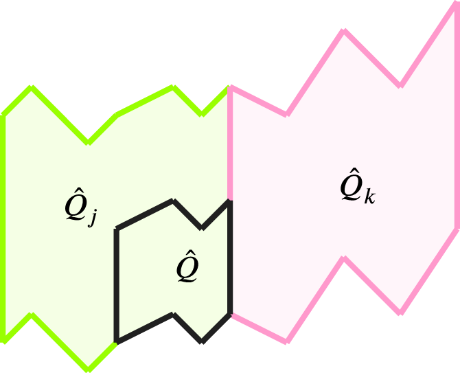


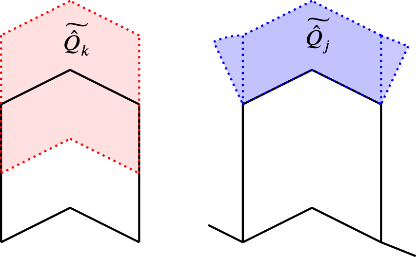


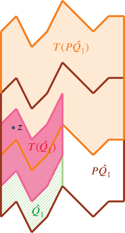


 Open access