


1. Introduction
Heat sinks are ubiquitous in modern computing and telecommunications hardware. More generally, they are an enabling technology in the thermal management of all electronics and elsewhere. When the flow is unidirectional, generally the fins on them are nearly rectangular in cross-section, in which case the heat sink is referred to as a longitudinal-fin heat sink (LFHS). LFHSs are manufactured by various methods (extrusion, skiving, machining, etc.), each imposing constraints on, e.g. minimum fin spacing and thickness, maximum fin height-to-spacing ratio, materials and cost (Iyengar & Bar-Cohen Reference Iyengar and Bar-Cohen2007). Both air-cooled LFHSs (say, in a laptop) and water-cooled ones (say, in a ‘cold plate’ attached to a central processing unit, CPU, in a server blade) are common. The materials of LFHSs are most commonly aluminium or copper, although the former is incompatible with water.
The foundational study on laminar (forced) convection in an LFHS was published by Sparrow, Baliga & Patankar (Reference Sparrow, Baliga and Patankar1978). They considered fully developed flow and heat transfer and allowed for tip clearance between the top of the fins and an adiabatic shroud, but not for bypass flow around the sides of the LFHS. Viscous dissipation was assumed negligible and thermophysical properties were considered to be constant. Their key results pertained to an isothermal base, a valid assumption in modern applications when, as is common, the fins are attached to a vapour chamber. A key assumption invoked by Sparrow et al. (Reference Sparrow, Baliga and Patankar1978) was that, geometrically, the fins were considered to be vanishingly thin, and they neglected heat sink edge effects. Consequently, the fluid domain in one period was rectangular and, due to symmetry, its width was half the fin spacing as per figure 1. The dimensional fin spacing was $S^*$
, the fin height
$S^*$
, the fin height $H^*$
and the clearance
$H^*$
and the clearance $C^*$
. Their hydrodynamic results were provided via tabulations of the Poiseuille number (Po, or product of the friction factor and Reynolds number) as a function of the ratio of the fin-spacing-to-height ratio (
$C^*$
. Their hydrodynamic results were provided via tabulations of the Poiseuille number (Po, or product of the friction factor and Reynolds number) as a function of the ratio of the fin-spacing-to-height ratio ( $\varepsilon = S^*/H^*$
) and fin-clearance-to-height ratio (
$\varepsilon = S^*/H^*$
) and fin-clearance-to-height ratio ( $c = C^*/H^*$
).
$c = C^*/H^*$
).
Schematic cross-section of the periodic fin array (a) considered here and by Sparrow et al. (Reference Sparrow, Baliga and Patankar1978); and the dimensionless single period domain $\mathcal{D}$
(b).
$\mathcal{D}$
(b).

In the thermal problem, Sparrow et al. (Reference Sparrow, Baliga and Patankar1978) assumed that the Biot number based on the thickness of the fins was small; therefore, temperature varied only along its height. Importantly, the conjugate thermal problem (where the convection problem is coupled to a conduction problem in the fin) was solved by matching temperature and balancing the net heat conduction rate along a differential height of the fin with the heat rate into the fluid along the fin–fluid interface. In addition, heat transfer between the prime surface (between fins) and the fluid was captured. The local Nusselt numbers ( ${Nu}$
) along the fin and prime surface were provided as a function of non-dimensional distance
${Nu}$
) along the fin and prime surface were provided as a function of non-dimensional distance $x$
(along the prime surface) or
$x$
(along the prime surface) or $y$
(along the fin),
$y$
(along the fin), $\varepsilon$
,
$\varepsilon$
, $c$
and a dimensionless fin conduction parameter
$c$
and a dimensionless fin conduction parameter $\Omega$
defined as
$\Omega$
defined as
 \begin{equation} \Omega = \frac {k_{\!{f}}}{k}\frac {t^*}{2H^*}, \end{equation}
where $k_{\!{f}}$
is the thermal conductivity of the fin and
$k_{\!{f}}$
is the thermal conductivity of the fin and $k$
is that of the fluid, with
$k$
is that of the fluid, with $t^*$
the thickness of the fin. The fin becomes isothermal as
$t^*$
the thickness of the fin. The fin becomes isothermal as $\Omega \rightarrow \infty$
. They further provide a Nusselt number averaged over the prime surface and fin,
$\Omega \rightarrow \infty$
. They further provide a Nusselt number averaged over the prime surface and fin, $\overline {{Nu}}$
, that is independent of
$\overline {{Nu}}$
, that is independent of $x$
and
$x$
and $y$
, and a key engineering parameter. A key conclusion of Sparrow et al. (Reference Sparrow, Baliga and Patankar1978) was that the ubiquitous assumption of a constant heat transfer coefficient along the prime surface and fin is generally invalid. Alas, it remains common today. In a subsequent and related study, Sparrow & Hsu (Reference Sparrow and Hsu1981) relaxed the assumptions of the fins being vanishingly thin in the hydrodynamic problem and the fin temperature being constant across its width. (Axial conduction remains neglected in the fin and the fluid as in our own analysis to follow). The effects on the Poiseuille number were modest in the parametric ranges considered for realistic heat sink geometries. Moreover, it was shown that the adiabatic fin tip assumption compares well with the case where convection from the fin tip is captured because this assumption causes a marked increase in heat transfer near the tip.
$y$
, and a key engineering parameter. A key conclusion of Sparrow et al. (Reference Sparrow, Baliga and Patankar1978) was that the ubiquitous assumption of a constant heat transfer coefficient along the prime surface and fin is generally invalid. Alas, it remains common today. In a subsequent and related study, Sparrow & Hsu (Reference Sparrow and Hsu1981) relaxed the assumptions of the fins being vanishingly thin in the hydrodynamic problem and the fin temperature being constant across its width. (Axial conduction remains neglected in the fin and the fluid as in our own analysis to follow). The effects on the Poiseuille number were modest in the parametric ranges considered for realistic heat sink geometries. Moreover, it was shown that the adiabatic fin tip assumption compares well with the case where convection from the fin tip is captured because this assumption causes a marked increase in heat transfer near the tip.
Karamanis & Hodes (Reference Karamanis and Hodes2016), albeit restricting their attention to fully shrouded LFHSs (i.e. $c=0$
), discuss relevant studies subsequent to those by Sparrow et al. (Reference Sparrow, Baliga and Patankar1978), including representative ones pertaining to the conjugate problem. Additionally, they provide a procedure using the formulation by Sparrow et al. (Reference Sparrow, Baliga and Patankar1978) to find the unique combination of fin spacing, thickness and length which minimise the thermal resistance of an LFHS for a prescribed pressure drop driving the flow through it, fin height and fluid-to-solid thermal conductivity ratio. The engineering parameters Po and
$c=0$
), discuss relevant studies subsequent to those by Sparrow et al. (Reference Sparrow, Baliga and Patankar1978), including representative ones pertaining to the conjugate problem. Additionally, they provide a procedure using the formulation by Sparrow et al. (Reference Sparrow, Baliga and Patankar1978) to find the unique combination of fin spacing, thickness and length which minimise the thermal resistance of an LFHS for a prescribed pressure drop driving the flow through it, fin height and fluid-to-solid thermal conductivity ratio. The engineering parameters Po and $\overline {{Nu}}$
suffice for this. Dense tabulations of them relevant to the optimisation of the geometry of LFHSs when the fluid-to-solid thermal conductivity ratio is that of air-to-copper, air-to-aluminium, water-to-copper and water-to-silicon are provided by Karamanis (Reference Karamanis2015).
$\overline {{Nu}}$
suffice for this. Dense tabulations of them relevant to the optimisation of the geometry of LFHSs when the fluid-to-solid thermal conductivity ratio is that of air-to-copper, air-to-aluminium, water-to-copper and water-to-silicon are provided by Karamanis (Reference Karamanis2015).
Subsequent research by Karamanis & Hodes (2019a), again for the fully shrouded case ( $C^*=0$
), considered simultaneously developing flow through an LFHS and relaxed the low Biot number assumption, thereby accounting for temperature variation also across the fin’s thickness. Then, the Poiseuille number depends explicitly on the fin thickness-to-height ratio (
$C^*=0$
), considered simultaneously developing flow through an LFHS and relaxed the low Biot number assumption, thereby accounting for temperature variation also across the fin’s thickness. Then, the Poiseuille number depends explicitly on the fin thickness-to-height ratio ( $t=t^*/H^*$
), as well as an additional parameter, i.e.
$t=t^*/H^*$
), as well as an additional parameter, i.e. $L^+ = L^*/ (D_{{h}}{Re}_{D_{{h}}})$
as per numerical results by Curr, Sharma & Tatchell (Reference Curr, Sharma and Tatchell1972) and, subsequently, many others (Shah & London Reference Shah and London1978). Here
$L^+ = L^*/ (D_{{h}}{Re}_{D_{{h}}})$
as per numerical results by Curr, Sharma & Tatchell (Reference Curr, Sharma and Tatchell1972) and, subsequently, many others (Shah & London Reference Shah and London1978). Here $L^*$
is the streamwise channel length, and
$L^*$
is the streamwise channel length, and $Re_{D_h}$
is the Reynolds number based on the hydraulic diameter
$Re_{D_h}$
is the Reynolds number based on the hydraulic diameter $D_h$
. Thus, Karamanis & Hodes (2019a) provide
$D_h$
. Thus, Karamanis & Hodes (2019a) provide $\overline {{Nu}}$
as a function of
$\overline {{Nu}}$
as a function of $\varepsilon$
,
$\varepsilon$
, $t$
,
$t$
, $k/k_{\!{f}}$
,
$k/k_{\!{f}}$
, $L^+$
,
$L^+$
, $Re_{D_{{h}}}$
and
$Re_{D_{{h}}}$
and ${Pr}$
(the Prandtl number). Finally, Karamanis & Hodes (Reference Karamanis and Hodes2019b
) combined the results for Po and
${Pr}$
(the Prandtl number). Finally, Karamanis & Hodes (Reference Karamanis and Hodes2019b
) combined the results for Po and $\overline {{Nu}}$
from the foregoing studies with flow network modelling and multi-variable optimisation to find the optimal fin thickness, spacing, height and length for an array of heat sinks in a circuit pack such as a blade server, laptop or rack-mountable electronics or optoelectronics. Since then, there have been other numerical studies reporting optimal heat sink geometries. Representatively, Martin et al. (Reference Martin, Valeije, Sastre and Velazquez2022) and Sun, Ismail & Mustaffa (Reference Sun, Ismail and Mustaffa2025) optimised the aspect ratio of the ducts by a brute-force numerical method over a limited parameter space, with Sun et al. (Reference Sun, Ismail and Mustaffa2025) employing machine learning optimisation techniques.
$\overline {{Nu}}$
from the foregoing studies with flow network modelling and multi-variable optimisation to find the optimal fin thickness, spacing, height and length for an array of heat sinks in a circuit pack such as a blade server, laptop or rack-mountable electronics or optoelectronics. Since then, there have been other numerical studies reporting optimal heat sink geometries. Representatively, Martin et al. (Reference Martin, Valeije, Sastre and Velazquez2022) and Sun, Ismail & Mustaffa (Reference Sun, Ismail and Mustaffa2025) optimised the aspect ratio of the ducts by a brute-force numerical method over a limited parameter space, with Sun et al. (Reference Sun, Ismail and Mustaffa2025) employing machine learning optimisation techniques.
More recently, the hydrodynamic problem with ( $c\gt 0$
) or without clearance (
$c\gt 0$
) or without clearance ( $c=0$
) was revisited by Miyoshi et al. (Reference Miyoshi, Kirk, Hodes and Crowdy2024). They considered the limit of small fin spacing
$c=0$
) was revisited by Miyoshi et al. (Reference Miyoshi, Kirk, Hodes and Crowdy2024). They considered the limit of small fin spacing $\varepsilon \ll 1$
, which is typical in practice – see table 1. For example, Iyengar & Bar-Cohen (Reference Iyengar and Bar-Cohen2007) report the minimum values to range from
$\varepsilon \ll 1$
, which is typical in practice – see table 1. For example, Iyengar & Bar-Cohen (Reference Iyengar and Bar-Cohen2007) report the minimum values to range from $1/60$
(bonding) up to
$1/60$
(bonding) up to $1/6$
(die casting), or approximately
$1/6$
(die casting), or approximately $\varepsilon \approx 0.015{-}0.15$
. Although no clearance is ideal (
$\varepsilon \approx 0.015{-}0.15$
. Although no clearance is ideal ( $c=0$
), finite clearance (
$c=0$
), finite clearance ( $c\gt 0$
) is common, with the range of
$c\gt 0$
) is common, with the range of $c$
being highly variable. It may be as low as, say, 0.01, when a small gap is left between fin tips and an adjacent circuit board to accommodate thermal expansion. On the other hand, for lower power components, flow bypass is common and the clearance may exceed the fin height
$c$
being highly variable. It may be as low as, say, 0.01, when a small gap is left between fin tips and an adjacent circuit board to accommodate thermal expansion. On the other hand, for lower power components, flow bypass is common and the clearance may exceed the fin height $(c \gt 1)$
. In the small
$(c \gt 1)$
. In the small $\varepsilon$
limit, Miyoshi et al. (Reference Miyoshi, Kirk, Hodes and Crowdy2024) presented new flow solutions and
$\varepsilon$
limit, Miyoshi et al. (Reference Miyoshi, Kirk, Hodes and Crowdy2024) presented new flow solutions and ${Po}$
formulas for a range of clearances, using complex conformal maps and matched asymptotic expansions.
${Po}$
formulas for a range of clearances, using complex conformal maps and matched asymptotic expansions.
Typical parameter values possible in practical LFHSs. The $\varepsilon$
values are the minimum for different manufacturing methods as reported by Iyengar & Bar–Cohen (Reference Iyengar and Bar-Cohen2007). We also used corresponding fin thicknesses
$\varepsilon$
values are the minimum for different manufacturing methods as reported by Iyengar & Bar–Cohen (Reference Iyengar and Bar-Cohen2007). We also used corresponding fin thicknesses $(t^*)$
therein to estimate
$(t^*)$
therein to estimate $\Omega$
.
$\Omega$
. $Re$
ranges from experiments Reyes et al. (Reference Reyes, Arias, Velazquez and Vega2011) (water), Sparrow & Kadle (Reference Sparrow and Kadle1986) (air).
$Re$
ranges from experiments Reyes et al. (Reference Reyes, Arias, Velazquez and Vega2011) (water), Sparrow & Kadle (Reference Sparrow and Kadle1986) (air).

The analysis of Miyoshi et al. (Reference Miyoshi, Kirk, Hodes and Crowdy2024) was limited to the hydrodynamic problem. In this companion paper we consider the corresponding conjugate thermal problem (i.e. precisely the one numerically solved by Sparrow et al. Reference Sparrow, Baliga and Patankar1978) in the limit of small fin spacing ( $\varepsilon \ll 1$
) with finite clearance (
$\varepsilon \ll 1$
) with finite clearance ( $c \gt 0$
). We derive explicit formulas for the coupled temperature fields in the fluid and the fin, and the local and overall heat transfer quantities as a function of
$c \gt 0$
). We derive explicit formulas for the coupled temperature fields in the fluid and the fin, and the local and overall heat transfer quantities as a function of $\varepsilon$
,
$\varepsilon$
, $c$
and
$c$
and $\Omega$
, thereby replacing many of the numerical results of Sparrow et al. (Reference Sparrow, Baliga and Patankar1978). To validate these formulas, we compare them with our numerical solutions of the full model, as well as the (equivalently) results of Sparrow et al. (Reference Sparrow, Baliga and Patankar1978). Two approximations (leading order and higher order, respectively) for the average Nusselt number are found to take the simple forms
$\Omega$
, thereby replacing many of the numerical results of Sparrow et al. (Reference Sparrow, Baliga and Patankar1978). To validate these formulas, we compare them with our numerical solutions of the full model, as well as the (equivalently) results of Sparrow et al. (Reference Sparrow, Baliga and Patankar1978). Two approximations (leading order and higher order, respectively) for the average Nusselt number are found to take the simple forms
 \begin{align} \overline {{Nu}}^{(0)} &=\frac {2.4304\,\varepsilon }{c(2+\varepsilon)} +O(\varepsilon ^2), \end{align}
 \begin{align} \overline {{Nu}}^{(1)} &= \frac {\varepsilon }{c(2 + \varepsilon)} \displaystyle {\left [2.4304 - \frac {\varepsilon }{c}\left ( 0.5362 + \frac {2.6449}{\Omega }\right)\right]} +O(\varepsilon ^3), \end{align}
and their comparisons with numerical solutions are summarised in figures 9, 10 and 11. The numerical constants in the above, shown to 4 decimal places, are readily calculated to arbitrary precision.
We note that, in practice, heat sinks on low-power components in circuit packs, such as voltage regulators, metal–oxide–semiconductor field-effect transistors (MOSFETs) and memory, are not fully shrouded, i.e. $c$
in figure 1 is finite. Minimising the cost, weight, size, etc. of them, albeit a secondary consideration in an overall thermal management solution, requires knowledge of how the conjugate Nusselt numbers depend upon the solid–fluid combination and the geometry of the heat sink via
$c$
in figure 1 is finite. Minimising the cost, weight, size, etc. of them, albeit a secondary consideration in an overall thermal management solution, requires knowledge of how the conjugate Nusselt numbers depend upon the solid–fluid combination and the geometry of the heat sink via $\Omega$
,
$\Omega$
, $\varepsilon$
and
$\varepsilon$
and $c$
. Moreover, it further depends upon the corresponding Poiseuille numbers, which in turn, depend upon
$c$
. Moreover, it further depends upon the corresponding Poiseuille numbers, which in turn, depend upon $\varepsilon$
and
$\varepsilon$
and $c$
, as per our companion study (Miyoshi et al. Reference Miyoshi, Kirk, Hodes and Crowdy2024). Indeed, the caloric resistance of a heat sink, i.e. that associated with the bulk temperature rise of the fluid, is also important (Karamanis & Hodes 2016). Furthermore, the inlet fluid velocity and temperature profiles to the heat sinks on the high-power components (where
$c$
, as per our companion study (Miyoshi et al. Reference Miyoshi, Kirk, Hodes and Crowdy2024). Indeed, the caloric resistance of a heat sink, i.e. that associated with the bulk temperature rise of the fluid, is also important (Karamanis & Hodes 2016). Furthermore, the inlet fluid velocity and temperature profiles to the heat sinks on the high-power components (where $c$
is normally 0), such as central processing units (CPUs), are affected by the pressure drops and temperature rises as fluid flows through the heat sinks on low-power ones.
$c$
is normally 0), such as central processing units (CPUs), are affected by the pressure drops and temperature rises as fluid flows through the heat sinks on low-power ones.
Another practical consideration is whether or not the flow is hydrodynamically and thermally fully developed as assumed here. The values of $L^+$
corresponding to hydrodynamically fully developed flow in rectangular ducts (
$L^+$
corresponding to hydrodynamically fully developed flow in rectangular ducts ( $c=0$
) are well known, as per the aforementioned study by Curr et al. (Reference Curr, Sharma and Tatchell1972). Moreover, since the Prandtl numbers for air and water are approximately 0.7 and 7, respectively, when the flow is hydrodynamically fully developed, it may be assumed to be thermally fully developed. However, to our knowledge, development lengths for the problem when
$c=0$
) are well known, as per the aforementioned study by Curr et al. (Reference Curr, Sharma and Tatchell1972). Moreover, since the Prandtl numbers for air and water are approximately 0.7 and 7, respectively, when the flow is hydrodynamically fully developed, it may be assumed to be thermally fully developed. However, to our knowledge, development lengths for the problem when $c\gt 0$
have not been considered and is beyond the scope of the present study. In the case of
$c\gt 0$
have not been considered and is beyond the scope of the present study. In the case of $c=0$
, it is very common for hydrodynamically and thermally fully developed flow to be a valid assumption as per, e.g. in the direct liquid cooling of a CPU (Zhang et al. Reference Zhang, Hodes, Lower and Wilcoxon2015). Further, the Reynolds number
$c=0$
, it is very common for hydrodynamically and thermally fully developed flow to be a valid assumption as per, e.g. in the direct liquid cooling of a CPU (Zhang et al. Reference Zhang, Hodes, Lower and Wilcoxon2015). Further, the Reynolds number $Re$
(based on the hydraulic diameter) is commonly low enough for laminar flow, e.g. in the range
$Re$
(based on the hydraulic diameter) is commonly low enough for laminar flow, e.g. in the range $400 {-} 2600$
in water microchannel heat sinks (Reyes et al. Reference Reyes, Arias, Velazquez and Vega2011), but it can also be transitional or turbulent for air (Sparrow & Kadle Reference Sparrow and Kadle1986). Nonetheless, for fully developed laminar flow (which we provide formulas for in this paper), the conclusions of Sparrow et al. (Reference Sparrow, Baliga and Patankar1978), that tip clearance results in a significant reduction in heat transfer, have been qualitatively borne out by experimental works in subsequent decades (Reyes et al. Reference Reyes, Arias, Velazquez and Vega2011).
$400 {-} 2600$
in water microchannel heat sinks (Reyes et al. Reference Reyes, Arias, Velazquez and Vega2011), but it can also be transitional or turbulent for air (Sparrow & Kadle Reference Sparrow and Kadle1986). Nonetheless, for fully developed laminar flow (which we provide formulas for in this paper), the conclusions of Sparrow et al. (Reference Sparrow, Baliga and Patankar1978), that tip clearance results in a significant reduction in heat transfer, have been qualitatively borne out by experimental works in subsequent decades (Reyes et al. Reference Reyes, Arias, Velazquez and Vega2011).
The paper is structured as follows. The mathematical problem is formulated in § 2. A summary of the solutions to the flow and thermal problems in the narrow-fin-spacing limit ( $\varepsilon \ll 1$
) is presented in § 3. The Nusselt number definitions and formulas are given in § 4, and they are compared with numerical solutions in § 5, followed by conclusions in § 6.
$\varepsilon \ll 1$
) is presented in § 3. The Nusselt number definitions and formulas are given in § 4, and they are compared with numerical solutions in § 5, followed by conclusions in § 6.
2. Problem formulation
In this section we formulate the problem as given in Sparrow et al. (Reference Sparrow, Baliga and Patankar1978). A schematic of the shrouded heat sink is shown in figure 1, including all dimensional lengths (and their non-dimensional ratios). The fin array is periodic and aligned longitudinally with the flow direction. The fin thickness is assumed to be negligible compared with other lengths, except for the purpose of heat conduction along it. Throughout, an asterisk will denote that a variable or length is dimensional (thermophysical properties are always dimensional). We assume that the flow is hydrodynamically and thermally fully developed, and consider the coupled (conjugate) thermal problems in the fluid and fins simultaneously.
The flow is unidirectional in the $z^*$
direction. The velocity field,
$z^*$
direction. The velocity field, $w^*(x^*,y^*)$
, is governed by
$w^*(x^*,y^*)$
, is governed by
 \begin{align} \frac {\partial ^2 w^*}{\partial x^{*2}} + \frac {\partial ^2 w^*}{\partial y^{*2}} &= \frac {1}{\mu } \frac {\mathrm{d} p^*}{\mathrm{d} z^*} \quad \text{in } \mathcal{D}, \end{align}
where $\mu$
is the dynamic viscosity and
$\mu$
is the dynamic viscosity and $\mathrm{d} p^* / \mathrm{d} z^*$
is the constant pressure gradient. By periodicity, we restrict attention to a single fin period,
$\mathrm{d} p^* / \mathrm{d} z^*$
is the constant pressure gradient. By periodicity, we restrict attention to a single fin period, $\mathcal{D} = \{0\leqslant x^* \leqslant S^*, 0\leqslant y^* \leqslant H^* + C^*\}$
. The flow satisfies no slip (
$\mathcal{D} = \{0\leqslant x^* \leqslant S^*, 0\leqslant y^* \leqslant H^* + C^*\}$
. The flow satisfies no slip ( $w^*=0$
) on the fin (
$w^*=0$
) on the fin ( $x^*=0$
and
$x^*=0$
and $0\lt y^*\lt H^*$
), base (
$0\lt y^*\lt H^*$
), base ( $y^*\,{=}\,0$
) and shroud (
$y^*\,{=}\,0$
) and shroud ( $y^*=H^*$
), and symmetry (
$y^*=H^*$
), and symmetry ( $\partial w^*/\partial x^* = 0$
) along the centreline between adjacent fins (
$\partial w^*/\partial x^* = 0$
) along the centreline between adjacent fins ( $x^*=S^*/2)$
and above each fin (
$x^*=S^*/2)$
and above each fin ( $x^*=0$
and
$x^*=0$
and $H^*\lt y^*\lt H^* + C^*$
).
$H^*\lt y^*\lt H^* + C^*$
).
The thermal energy equation in the fluid takes the form
 \begin{align} w^* \frac {\partial T^*}{\partial z^*} &= \alpha \left ( \frac {\partial ^2 T^*}{\partial x^{*2}} + \frac {\partial ^2 T^*}{\partial y^{*2}}\right) \quad \text{in } \mathcal{D}, \end{align}
where $T^*(x^*,y^*,z^*)$
is the fluid temperature and
$T^*(x^*,y^*,z^*)$
is the fluid temperature and $\alpha$
is its thermal diffusivity. We assume that the base is isothermal, at temperature
$\alpha$
is its thermal diffusivity. We assume that the base is isothermal, at temperature $T_{{base}}^*$
; hence, the fully developed assumption implies
$T_{{base}}^*$
; hence, the fully developed assumption implies
 \begin{align} \frac {\partial T^*}{\partial z^*} &= \frac {T^*(x^*,y^*,z^*)-T_{{base}}^*}{T_{{b}}^*(z^*) - T_{{base}}^*}\frac {\mathrm{d} T_{{b}}^*}{\mathrm{d} z^*}, \end{align}
where
 \begin{align} T_{{b}}^* &= \frac {\int _{\mathcal{D}} w^*T^*\,\mathrm{d}A^*}{\int _{\mathcal{D}} w^*\,\mathrm{d}A^*}, \end{align}
is the bulk fluid temperature. Boundary conditions specifying an isothermal base, adiabatic shroud, and symmetry above the fins ( $x^*=0$
) and between them (
$x^*=0$
) and between them ( $x^*=S^*/2$
) are given by
$x^*=S^*/2$
) are given by
 \begin{align} T^* &= T_{{base}}^* \qquad \text{on } y^*=0, \end{align}
 \begin{align} \frac {\partial T^*}{\partial y^*} &= 0 \qquad\quad\ \ \ \text{on}\ y^*=H^* + C^*, \end{align}
 \begin{align} \frac {\partial T^*}{\partial x^*} &= 0 \qquad\quad\ \ \ \text{on}\ x^* = 0, \quad H^*\lt y^* \lt H^*+C^*, \end{align}
 \begin{align} \frac {\partial T^*}{\partial x^*} &= 0 \qquad\quad\ \ \ \text{on}\ x^* = S^*/2, \quad 0\lt y^* \lt H^*+C^*, \end{align}
respectively. On the fin surface, we have continuity of temperature and heat flux with the conduction problem within the fin. The Biot number based on fin thickness is assumed to be small enough that the temperature across its width is approximately constant, with significant temperature variations occurring only along its height. Performing an energy balance across half the width, $t^*$
, of the fin (only half is relevant to the domain considered), conduction up the fin is governed by the one-dimensional equation
$t^*$
, of the fin (only half is relevant to the domain considered), conduction up the fin is governed by the one-dimensional equation
 \begin{align} \frac {k_{\!{f}} t^*}{2} \frac {\mathrm{d}^2 T_{\!{f}}^*}{\mathrm{d}y^{*2}} &= -k \left. \frac {\partial T^*}{\partial x^*}\right |_{x^*=0},\qquad \text{for }0\lt y^*\lt H^*, \end{align}
where $T_{\!{f}}^*$
is the fin temperature. The sink term on the right-hand side corresponds to heat conducting (at each
$T_{\!{f}}^*$
is the fin temperature. The sink term on the right-hand side corresponds to heat conducting (at each $y^*$
location) out of the fin and into the fluid. We remark that the ‘small Biot number’ assumption can be translated explicitly into an assumption on the conductivity ratio
$y^*$
location) out of the fin and into the fluid. We remark that the ‘small Biot number’ assumption can be translated explicitly into an assumption on the conductivity ratio $k_{\!{f}}/k$
. Typically
$k_{\!{f}}/k$
. Typically $k_{\!{f}} /k$
will be large (e.g.
$k_{\!{f}} /k$
will be large (e.g. $O(10^4)$
for aluminium and air) and, mathematically, to allow conduction up the fin when taking the limit of small thickness (
$O(10^4)$
for aluminium and air) and, mathematically, to allow conduction up the fin when taking the limit of small thickness ( $t^*/H^* \ll 1$
) we must have
$t^*/H^* \ll 1$
) we must have $k_{\!{f}} /k = O((t^*/H^*)^{-1})$
or larger. (This can be shown rigorously by considering the limit
$k_{\!{f}} /k = O((t^*/H^*)^{-1})$
or larger. (This can be shown rigorously by considering the limit $t^*/H^*\to 0$
of the two-dimensional conduction problem in the fin, while taking the distinguished limit
$t^*/H^*\to 0$
of the two-dimensional conduction problem in the fin, while taking the distinguished limit $k_{\!{f}}/k = O((t^*/H^*)^{-1})$
so that the product
$k_{\!{f}}/k = O((t^*/H^*)^{-1})$
so that the product $k_{\!{f}}t^*/(2kH^*) = \Omega$
stays fixed) Or in terms of
$k_{\!{f}}t^*/(2kH^*) = \Omega$
stays fixed) Or in terms of $\Omega$
(given by (1.1)), this is equivalent to
$\Omega$
(given by (1.1)), this is equivalent to $\Omega = O(1)$
or larger. This assumption allows the temperature variations up the fin to be comparable to the temperature variations in the fluid.
$\Omega = O(1)$
or larger. This assumption allows the temperature variations up the fin to be comparable to the temperature variations in the fluid.
There is also temperature continuity between the fin and fluid
 \begin{align} T_{\!{f}}^* &= \left. T^*\right |_{x^*=0},\qquad \text{for }0\lt y^*\lt H^*. \end{align}
(Note, axial conduction in $z^*$
in the fin is also neglected for fully developed flow, as is typical for axially constant temperature boundary conditions – see (Shah & London Reference Shah and London1978, Chapter 2) – because the ratio of axial conduction to transverse conduction scales the same way in both the fin and fluid, and so both are negligible if the axial Péclet number is large). Of course, there is another identical fin at
$z^*$
in the fin is also neglected for fully developed flow, as is typical for axially constant temperature boundary conditions – see (Shah & London Reference Shah and London1978, Chapter 2) – because the ratio of axial conduction to transverse conduction scales the same way in both the fin and fluid, and so both are negligible if the axial Péclet number is large). Of course, there is another identical fin at $x^*=S^*$
with the same temperature
$x^*=S^*$
with the same temperature $T_{\!{f}}^*$
, but in practice we enforce symmetry down the centreline at
$T_{\!{f}}^*$
, but in practice we enforce symmetry down the centreline at $x^*=S^*/2$
instead.
$x^*=S^*/2$
instead.
Finally, the isothermal condition at the base and adiabatic condition at the tip (due to its negligible surface area) are, respectively,
 \begin{align} T_{\!{f}}^* &= T_{{base}}^*,\quad \text{at } y^*=0, \end{align}
 \begin{align} \frac {\mathrm{d} T_{\!{f}}^*}{\mathrm{d}y^{*}} &= 0,\quad\quad\ \ \text{at}\ y^*=H^*. \end{align}
2.1. Non-dimensional equations
The flow problem (2.1) is non-dimensionalised by scaling $x^*$
and
$x^*$
and $y^*$
with
$y^*$
with $H^*$
and the velocity with
$H^*$
and the velocity with $(- \partial p^* / \partial z^*)H^{*2}/\mu$
, i.e. introducing
$(- \partial p^* / \partial z^*)H^{*2}/\mu$
, i.e. introducing
 \begin{align} x &= x^*/H^*, & y &= y^*/H^*, & w = \frac {\mu }{(- \mathrm{d} p^* / \mathrm{d} z^*)H^{*2}}w^*, \end{align}
resulting in a non-dimensional streamwise momentum (Poisson) equation of the form
 \begin{align} \frac {\partial ^2 w}{\partial x^2} + \frac {\partial ^2 w}{\partial y^2} &= - 1 \quad \text{in } \mathcal{D}. \end{align}
It is subjected to the boundary conditions
 \begin{align} w &= 0 \qquad \text{on } y=0,\, 1 + c, \end{align}
 \begin{align} w &= 0 \qquad \text{on } x=0,\varepsilon,\quad 0\lt y \lt 1, \end{align}
 \begin{align} \frac {\partial w}{\partial x} &= 0 \qquad \text{on } x = 0,\varepsilon, \quad 1\lt y \lt 1+c, \end{align}
where the non-dimensional geometric parameters are then $\varepsilon = S^*/H^*$
, the ratio of fin spacing to fin height, and
$\varepsilon = S^*/H^*$
, the ratio of fin spacing to fin height, and $c = C^*/H^*$
, the ratio of clearance to fin height.
$c = C^*/H^*$
, the ratio of clearance to fin height.
As in Sparrow et al. (Reference Sparrow, Baliga and Patankar1978), we define a non-dimensional temperature field in the fluid as
 \begin{align} T &= \frac {T^*-T_{{base}}^*}{T_{{b}}^* - T_{{base}}^*}, \end{align}
and a non-dimensional streamwise coordinate as
 \begin{align} z &= \frac {\alpha z^*}{\overline {w}^*H^{*2}}, \end{align}
where $\overline {w}^*$
is the average velocity
$\overline {w}^*$
is the average velocity
 \begin{align} \overline {w}^* &= \frac {1}{S^*(H^*+C^*)}\int _{\mathcal{D}} w^* \mathrm{d}A^*. \end{align}
Expressing (2.2) in non-dimensional form, we have
 \begin{align} \lambda \mathcal{W} T &= \frac {\partial ^2 T}{\partial x^2} + \frac {\partial ^2 T}{\partial y^2} \quad \text{in } \mathcal{D}, \end{align}
where we have defined $\mathcal{W} = w/\overline {w}$
, and
$\mathcal{W} = w/\overline {w}$
, and
 \begin{align} \lambda &= \frac {1}{T_{{b}}^* - T_{{base}}^*}\frac {\mathrm{d} T_{{b}}^*}{\mathrm{d} z}, \end{align}
is the non-dimensional exponential decay rate of $T_{{b}}^* - T_{{base}}^*$
, which is a negative constant due to the fully developed assumption. This constant is fixed by enforcing the definition of the bulk temperature, which in non-dimensional terms must be equal to one, i.e.
$T_{{b}}^* - T_{{base}}^*$
, which is a negative constant due to the fully developed assumption. This constant is fixed by enforcing the definition of the bulk temperature, which in non-dimensional terms must be equal to one, i.e.
 \begin{align} \frac {1}{\varepsilon (1+c)}\int _{\mathcal{D}} \mathcal{W}T\, \mathrm{d}A &= 1. \end{align}
The corresponding boundary conditions (2.5)–(2.8) become
 \begin{align} T &= 0 \qquad \text{on } y=0, \end{align}
 \begin{align} \frac {\partial T}{\partial y} &= 0 \qquad \text{on } y=1+c, \\[-12pt] \nonumber \end{align}
 \begin{align} \frac {\partial T}{\partial x} &= 0 \qquad \text{on } x = 0, \quad 1\lt y \lt 1+c, \\[-12pt] \nonumber \end{align}
 \begin{align} \frac {\partial T}{\partial x} &= 0 \qquad \text{on } x = \varepsilon /2, \quad 0\lt y \lt 1+c. \end{align}
Defining the non-dimensional fin temperature $T_{\!{f}}$
as in (2.18), where
$T_{\!{f}}$
as in (2.18), where $T$
and
$T$
and $T^*$
are replaced by
$T^*$
are replaced by $T_{\!{f}}$
and
$T_{\!{f}}$
and $T^*_{\!{f}}$
, the thermal problem in the fin, (2.9)–(2.12), becomes
$T^*_{\!{f}}$
, the thermal problem in the fin, (2.9)–(2.12), becomes
 \begin{align} \Omega \frac {\mathrm{d}^2 T_{\!{f}}}{\mathrm{d}y^{2}} &= - \left. \frac {\partial T}{\partial x}\right |_{x=0}, \quad \text{for }0\lt y\lt 1,\\[-10pt]\nonumber \end{align}
 \begin{align} T_{\!{f}} &= \left. T\right |_{x=0}, \quad \text{for }0\lt y\lt 1,\\[-10pt]\nonumber \end{align}
 \begin{align} T_{\!{f}} &= 0,\quad \text{at } y=0, \\[-10pt]\nonumber \end{align}
 \begin{align} \frac {\mathrm{d} T_{\!{f}}}{\mathrm{d}y} &= 0,\quad \text{at } y=1, \end{align}
where $\Omega$
(given by 1.1) is the product of the fin-to-fluid conductivity ratio and the fin’s (small) thickness-to-height ratio. The limit
$\Omega$
(given by 1.1) is the product of the fin-to-fluid conductivity ratio and the fin’s (small) thickness-to-height ratio. The limit $\Omega \rightarrow \infty$
corresponds to an isothermal fin, where
$\Omega \rightarrow \infty$
corresponds to an isothermal fin, where $T=0$
along the entire fin surface.
$T=0$
along the entire fin surface.
The above non-dimensional system of equations can be solved in their current form, but for consistency with the literature and to yield a more convenient equation for $\lambda$
, we instead solve for the scaled temperatures
$\lambda$
, we instead solve for the scaled temperatures
 \begin{align} \phi &= \frac {T}{\lambda }, & \phi _{\!{f}} &= \frac {T_{\!{f}}}{\lambda }. \end{align}
Under this transformation, all equations and boundary conditions remain unchanged ( $T$
and
$T$
and $T_{\!{f}}$
replaced with
$T_{\!{f}}$
replaced with $\phi$
and
$\phi$
and $\phi _{\!{f}}$
, respectively), except for the integral condition (2.23) which becomes
$\phi _{\!{f}}$
, respectively), except for the integral condition (2.23) which becomes
 \begin{align} \lambda &= \frac {\varepsilon (1+c)}{\displaystyle { \int _{\mathcal{D}} \mathcal{W}\phi \, \mathrm{d}A }}, \end{align}
with $\lambda$
now appearing explicitly.
$\lambda$
now appearing explicitly.
3. Solutions in the small-fin-spacing limit
We consider the flow and conjugate thermal problems, i.e. (2.14)–(2.17) and (2.21)–(2.33), respectively, in the geometric limit where the fin spacing is small in comparison with the fin height, i.e. $\varepsilon = S^*/H^* \ll 1$
. This is typical of real heat sinks by design, to increase the total surface area for heat transfer; see table 1 and, e.g. the photographs of heat sinks used in the thermal management of electronics in Iyengar & Bar-Cohen (Reference Iyengar and Bar-Cohen2007). Importantly, we will further assume that the non-dimensional tip clearance,
$\varepsilon = S^*/H^* \ll 1$
. This is typical of real heat sinks by design, to increase the total surface area for heat transfer; see table 1 and, e.g. the photographs of heat sinks used in the thermal management of electronics in Iyengar & Bar-Cohen (Reference Iyengar and Bar-Cohen2007). Importantly, we will further assume that the non-dimensional tip clearance, $c=C^*/H^*$
, will remain of order 1 as we take
$c=C^*/H^*$
, will remain of order 1 as we take $\varepsilon \to 0$
. This is common for lower-power components on a printed wiring board (say, voltage regulators) which use smaller heat sinks than higher-power ones (say, a central processing unit). The hydrodynamic problem in this limit has already been considered by Miyoshi et al. (Reference Miyoshi, Kirk, Hodes and Crowdy2024), and we present here corresponding solutions for the thermal problem. It is instructive to summarise the hydrodynamic solution first, before presenting a summary of the temperature solution. The full derivation of the temperature solution can be found in Appendix A.
$\varepsilon \to 0$
. This is common for lower-power components on a printed wiring board (say, voltage regulators) which use smaller heat sinks than higher-power ones (say, a central processing unit). The hydrodynamic problem in this limit has already been considered by Miyoshi et al. (Reference Miyoshi, Kirk, Hodes and Crowdy2024), and we present here corresponding solutions for the thermal problem. It is instructive to summarise the hydrodynamic solution first, before presenting a summary of the temperature solution. The full derivation of the temperature solution can be found in Appendix A.
3.1. Summary of hydrodynamic solution
It is convenient to rescale the $x$
coordinate by defining
$x$
coordinate by defining $X=x/\varepsilon$
, so that the problem domain is independent of
$X=x/\varepsilon$
, so that the problem domain is independent of $\varepsilon$
. Then, (2.14)–(2.17) become
$\varepsilon$
. Then, (2.14)–(2.17) become
 \begin{align} \frac {1}{\varepsilon ^2}\frac {\partial ^2 w}{\partial X^2} + \frac {\partial ^2 w}{\partial y^2} &= -1 \quad \text{in } \mathcal{D}=\{0\lt X\lt 1,\,0\lt y\lt 1+c\}, \end{align}
 \begin{align} w &= 0 \qquad \text{on } y=0,\, 1 + c, \end{align}
 \begin{align} w &= 0 \qquad \text{on } X=0,1,\quad 0\lt y \lt 1, \end{align}
 \begin{align} \frac {\partial w}{\partial X} &= 0 \qquad \text{on } X = 0,1,\quad 1\lt y \lt 1+c. \end{align}
Considering now $\varepsilon \to 0$
, the asymptotic solution takes a different form depending on the region in the domain. Employing matched asymptotic expansions, the domain decomposes into a gap region (
$\varepsilon \to 0$
, the asymptotic solution takes a different form depending on the region in the domain. Employing matched asymptotic expansions, the domain decomposes into a gap region ( $1 \lt y \lt 1 + c$
) above the fins, a fin region (
$1 \lt y \lt 1 + c$
) above the fins, a fin region ( $0 \lt y \lt 1$
) between the fins (but at least a distance
$0 \lt y \lt 1$
) between the fins (but at least a distance $O(\varepsilon)$
away from their base or tips) and a short tip region near the fin tips (
$O(\varepsilon)$
away from their base or tips) and a short tip region near the fin tips ( $y - 1 = O(\varepsilon)$
) that transitions between them. There is also a small base region, (
$y - 1 = O(\varepsilon)$
) that transitions between them. There is also a small base region, ( $y=O(\varepsilon)$
) but it is not relevant to the thermal analysis (see Miyoshi et al. Reference Miyoshi, Kirk, Hodes and Crowdy2024 for more details). A schematic of the different regions and the resulting problems within each, is shown in figure 2.
$y=O(\varepsilon)$
) but it is not relevant to the thermal analysis (see Miyoshi et al. Reference Miyoshi, Kirk, Hodes and Crowdy2024 for more details). A schematic of the different regions and the resulting problems within each, is shown in figure 2.
Asymptotic structure of the domain showing the gap, tip and fin regions, and the behaviour of the velocity and temperature expansions in each region (the region close to the base, $y=O(\varepsilon)$
, is not considered here).
$y=O(\varepsilon)$
, is not considered here).

3.1.1. Gap region: $1 \lt y \leqslant 1 + c$

In the gap region above the fins, a regular expansion $w = w_0 + \varepsilon w_1 + \cdots$
for
$w = w_0 + \varepsilon w_1 + \cdots$
for $\varepsilon \ll 1$
leads to the result that
$\varepsilon \ll 1$
leads to the result that $w$
is independent of
$w$
is independent of $X$
(i.e. only a function of
$X$
(i.e. only a function of $y$
) to all algebraic orders. Thus the unit pressure gradient, and the no-slip condition on the shroud (
$y$
) to all algebraic orders. Thus the unit pressure gradient, and the no-slip condition on the shroud ( $y=1+c$
) lead to a Poiseuille-type parabolic flow profile. The leading-order flow is
$y=1+c$
) lead to a Poiseuille-type parabolic flow profile. The leading-order flow is
 \begin{align} w_0(y) &= -{\scriptstyle \frac{1}{2}}(y-1)(y-1-c), \end{align}
and the $O(\varepsilon)$
correction is a shear flow
$O(\varepsilon)$
correction is a shear flow
 \begin{align} w_1(y) &= -\frac {\log 2}{2\pi }(y - 1 - c), \end{align}
that is induced by the non-parabolic flow in the tip region, which is discussed after we present the solution in the fin region.
3.1.2. Fin region:
$0 \lt y \lt 1$

Denoting the solution in this region by $\tilde {w}$
, a regular expansion
$\tilde {w}$
, a regular expansion $\tilde {w} = \tilde {w}_0 +\varepsilon \tilde {w}_1 + \cdots$
leads this time to a Poiseuille flow but with variation in the
$\tilde {w} = \tilde {w}_0 +\varepsilon \tilde {w}_1 + \cdots$
leads this time to a Poiseuille flow but with variation in the $X$
direction. This is because the flow must satisfy no-slip conditions on the fins at
$X$
direction. This is because the flow must satisfy no-slip conditions on the fins at $X=0$
and 1. The result is that
$X=0$
and 1. The result is that
 \begin{align} \tilde {w} &= {\scriptstyle \frac {1}{2}}\varepsilon ^2 X(1-X) + \cdots, \end{align}
where any higher orders are beyond all algebraic powers, and thus are exponentially small in $\varepsilon$
.
$\varepsilon$
.
Interestingly, the flow in both the gap and fin regions is parabolic, but with variations oriented perpendicularly to one another. The transition between the two solutions takes place in the tip region, where the solution varies in both the $X$
and
$X$
and $y$
directions.
$y$
directions.
The no-slip condition at the bottom of the domain, $y=0$
, can be easily satisfied by the inclusion of a simple series, which is exponentially small unless
$y=0$
, can be easily satisfied by the inclusion of a simple series, which is exponentially small unless $y=O(\varepsilon)$
, i.e. close to the domain bottom. The modified solution is (Miyoshi et al. Reference Miyoshi, Kirk, Hodes and Crowdy2024)
$y=O(\varepsilon)$
, i.e. close to the domain bottom. The modified solution is (Miyoshi et al. Reference Miyoshi, Kirk, Hodes and Crowdy2024)
 \begin{align} \tilde {w}(X,y) &= \frac {1}{2}\varepsilon ^2 X(1-X) - 4\varepsilon ^2 \sum _{n=1,3,\ldots }\frac { \mathrm{e}^{-n\pi y/\varepsilon }\sin n\pi X}{n^3\pi ^3}. \end{align}
This is typically only relevant for visualising the flow field, since the effect of the base region on the average velocity is negligible.
3.1.3. Tip region:
$y - 1 = O(\varepsilon)$

Near the fin tips, i.e. an $O(\varepsilon)$
distance away, the variation in
$O(\varepsilon)$
distance away, the variation in $X$
becomes important; therefore, we introduce the inner variable
$X$
becomes important; therefore, we introduce the inner variable $Y = (y-1)/\varepsilon$
which is
$Y = (y-1)/\varepsilon$
which is $O(1)$
in this region, and we denote the solution here by
$O(1)$
in this region, and we denote the solution here by $w = W(X,Y)$
.
$w = W(X,Y)$
.
It turns out that asymptotic matching with the gap region above ( $Y \to +\infty$
) implies that the solution is
$Y \to +\infty$
) implies that the solution is $O(\varepsilon)$
here at leading order
$O(\varepsilon)$
here at leading order
 \begin{align} W = \varepsilon W_1(X,Y) + O(\varepsilon ^2), \end{align}
and $W_1(X,Y)$
(from (3.1), (3.3) and (3.4)) satisfies in the infinite strip
$W_1(X,Y)$
(from (3.1), (3.3) and (3.4)) satisfies in the infinite strip $\mathcal{D}_{{tip}} = \{0\,{\lt}\, X\,{\lt}\,1,\,-\infty\,{\lt}\,Y\,{\lt}\,\infty\}$
 \begin{align} \nabla _{XY}^2 W_1 &= 0 \qquad \text{in } \mathcal{D}_{{tip}}, \end{align}
 \begin{align} W_1 &= 0 \qquad \text{on } X=0,1,\quad Y \lt 0, \end{align}
 \begin{align} \frac {\partial W_1}{\partial X} &= 0 \qquad \text{on } X = 0,1,\quad 0\lt Y, \end{align}
where $\nabla _{XY}^2 = \partial ^2/\partial X^2 + \partial ^2/\partial Y^2$
, and the asymptotic matching conditions
$\nabla _{XY}^2 = \partial ^2/\partial X^2 + \partial ^2/\partial Y^2$
, and the asymptotic matching conditions
 \begin{align} W_1 &\sim {\scriptstyle \frac {1}{2}}cY \quad \text{as } Y \to \infty, \end{align}
 \begin{align} W_1 &\to 0 \quad \text{as } Y \to -\infty. \end{align}
This has the convenient solution in terms of a complex variable (Miyoshi et al. Reference Miyoshi, Kirk, Hodes and Crowdy2024)
 \begin{align} W_1 &= -\frac {c}{2\pi }\log \left | \frac {\mathrm{e}^{\mathrm{i}\pi /4} - \tan ^{1/2}(\pi Z /2)}{\mathrm{e}^{\mathrm{i}\pi /4} + \tan ^{1/2}(\pi Z /2)} \right |,\qquad \text{where } Z = X+ \mathrm{i}Y. \end{align}
Notably, a constant term $c\log 2 / (2\pi)$
that perturbs the shear term
$c\log 2 / (2\pi)$
that perturbs the shear term $Y$
in the limit
$Y$
in the limit $Y \to \infty$
follows from this solution, since
$Y \to \infty$
follows from this solution, since
 \begin{align} W_1 &\sim \frac {1}{2}c\left [ Y + \frac {\log 2}{\pi } + O(\mathrm{e}^{-\pi Y}) \right] \quad \text{as } Y \to \infty, \end{align}
and matching at $O(\varepsilon)$
with the gap region solution leads to the response
$O(\varepsilon)$
with the gap region solution leads to the response $w_1$
, given by (3.6).
$w_1$
, given by (3.6).
3.1.4. Composite flow solutions
A pair of composite flow solutions valid through larger regions of the domain can be constructed by adding solutions in adjacent regions and subtracting the solution in the overlap region between them. When patched together in a piece-wise fashion, these can be used to construct a single global flow field if desired. We do so by splitting the domain into $y\geqslant 1$
and
$y\geqslant 1$
and $y\lt 1$
(i.e. at the fin tips), and then constructing a composite solution in each region separately.
$y\lt 1$
(i.e. at the fin tips), and then constructing a composite solution in each region separately.
A gap–tip composite (restricted to $1 \leqslant y \leqslant 1+c$
) is given by
$1 \leqslant y \leqslant 1+c$
) is given by
 \begin{align} w_{\textit{gap-tip}} &= \underbrace {w_0(y) + \varepsilon w_1(y)}_{\text{gap region}} + \underbrace {\varepsilon W_1 \left (X,\frac {y-1}{\varepsilon }\right)}_{\text{tip region}} - \underbrace {\frac { c}{2}\left (y - 1 + \frac {\varepsilon \log 2}{\pi }\right)}_{\text{gap-tip overlap}}, \nonumber \\ &= -\frac {1}{2}(y-1-c)\left (y-1 + \frac {\varepsilon \log 2}{\pi }\right) + \varepsilon W_1 \left (X,\frac {y-1}{\varepsilon }\right),\qquad 0\lt X\lt 1. \end{align}
On the other hand, a one-term composite (say restricted to $0 \leqslant y \lt 1$
) between the tip and fin regions is given simply by the tip solution
$0 \leqslant y \lt 1$
) between the tip and fin regions is given simply by the tip solution $\varepsilon W_1$
, since it matches with ‘zero’ appearing at that order in the fin region. Strictly, to bring in the
$\varepsilon W_1$
, since it matches with ‘zero’ appearing at that order in the fin region. Strictly, to bring in the $O(\varepsilon ^2)$
parabolic flow from the fin region one would require a two-term composite, but we do not possess a second term (of
$O(\varepsilon ^2)$
parabolic flow from the fin region one would require a two-term composite, but we do not possess a second term (of $O(\varepsilon ^2)$
) in the tip region. However, we can form an ad hoc composite with an
$O(\varepsilon ^2)$
) in the tip region. However, we can form an ad hoc composite with an $O(\varepsilon ^2)$
error in the tip region, by simply superimposing the tip and fin region solutions
$O(\varepsilon ^2)$
error in the tip region, by simply superimposing the tip and fin region solutions
 \begin{align} w_{\textit{tip-fin}} &= \underbrace {\varepsilon W_1 \left (X,\frac {y-1}{\varepsilon }\right)}_{\text{tip region}} + \underbrace {\tilde {w}(X,y)}_{\text{fin region}},\qquad 0\lt X\lt 1. \end{align}
This is used here purely to allow visualisation of the flow field in figures (i.e. Figure 3), and not for further detailed calculations. Here, $W_1(X,Y)$
is (3.15) and
$W_1(X,Y)$
is (3.15) and $\tilde {w}(X,y)$
is (3.8). Even though it has an
$\tilde {w}(X,y)$
is (3.8). Even though it has an $O(\varepsilon ^2)$
error in the tip region, the correct leading-order behaviour is exhibited in each of the (tip and fin) regions, and so the main flow features are retained.
$O(\varepsilon ^2)$
error in the tip region, the correct leading-order behaviour is exhibited in each of the (tip and fin) regions, and so the main flow features are retained.
The asymptotic piece-wise composite solution (3.17)–(3.18) for the velocity field $w(x,y)$
in one period (a), compared with the numerical velocity
$w(x,y)$
in one period (a), compared with the numerical velocity $w_{{num}}$
(b), with the local relative error
$w_{{num}}$
(b), with the local relative error $|w(x,y) -w_{{num}}(x,y)|/|w_{{num}}|$
(c). Geometric parameters are
$|w(x,y) -w_{{num}}(x,y)|/|w_{{num}}|$
(c). Geometric parameters are $\varepsilon =0.15$
and
$\varepsilon =0.15$
and $c=0.5$
. The asymptotic solution consists of two composites: one valid for
$c=0.5$
. The asymptotic solution consists of two composites: one valid for $y\geqslant 1$
, and one for
$y\geqslant 1$
, and one for $y\lt 1$
, and the separating line (
$y\lt 1$
, and the separating line ( $y=1$
) is shown as a dashed blue line. The fins (at
$y=1$
) is shown as a dashed blue line. The fins (at $0\leqslant y \leqslant 1$
,
$0\leqslant y \leqslant 1$
, $x=0,1$
) and base are shown in black.
$x=0,1$
) and base are shown in black.

3.1.5. Poiseuille number
The mean velocity is given by
 \begin{align} \overline {w} &= \frac {1}{1+c}\int _0^{1} \int _0^{1+c} w\,\mathrm{d}y\mathrm{d}X = \frac {c^3}{12(1+c)}\left [ 1 + \frac {\varepsilon \log 8}{\pi c} \right]+ O(\varepsilon ^2), \end{align}
where the contributions from the tip region (velocity of $O(\varepsilon)$
over a region of area
$O(\varepsilon)$
over a region of area $O(\varepsilon)$
) and fin region (velocity of
$O(\varepsilon)$
) and fin region (velocity of $O(\varepsilon ^2)$
over a region of area
$O(\varepsilon ^2)$
over a region of area $O(1)$
) are both
$O(1)$
) are both $O(\varepsilon ^2)$
, so
$O(\varepsilon ^2)$
, so $\overline {w}$
up to
$\overline {w}$
up to $O(\varepsilon)$
follows only from the gap solution (3.5), (3.6).
$O(\varepsilon)$
follows only from the gap solution (3.5), (3.6).
The friction factor is defined as (Sparrow et al. Reference Sparrow, Baliga and Patankar1978)
 \begin{align} f &= \frac {(- \mathrm{d}p^*/\mathrm{d}z^*) D_e^*}{\frac {1}{2}\rho \overline {w}^{*2}}, & D_e^* &= \frac {4(H^* + C^*)S^*}{2(H^* + S^*)}, \end{align}
and the Poiseuille number is then ${Po}=f{Re}$
where
${Po}=f{Re}$
where ${Re}=\rho \overline {w}^*D_e^*/\mu$
is the Reynolds number and
${Re}=\rho \overline {w}^*D_e^*/\mu$
is the Reynolds number and $\rho$
is the fluid density. In terms of non-dimensional quantities,
$\rho$
is the fluid density. In terms of non-dimensional quantities,
 \begin{align} {Po} = f{Re} &= \frac {8(1+c)^2\varepsilon ^2}{\overline {w}(1+\varepsilon)^2}. \end{align}
Substituting the asymptotic solution (3.19) for $\overline {w}$
results in the elementary expression (Miyoshi et al. Reference Miyoshi, Kirk, Hodes and Crowdy2024)
$\overline {w}$
results in the elementary expression (Miyoshi et al. Reference Miyoshi, Kirk, Hodes and Crowdy2024)
 \begin{align} {Po} &= \frac {96(1+c)^3\varepsilon ^2}{\displaystyle { c^2\left (c + \frac {\varepsilon \log 8}{\pi }\right)(1+\varepsilon)^2 }} + O(\varepsilon ^4),\quad \text{as }\varepsilon \to 0. \end{align}
This expression was compared with an exact solution valid for arbitrary $\varepsilon$
in Miyoshi et al. (Reference Miyoshi, Kirk, Hodes and Crowdy2024), and shown to be accurate to within 15 % if
$\varepsilon$
in Miyoshi et al. (Reference Miyoshi, Kirk, Hodes and Crowdy2024), and shown to be accurate to within 15 % if $\varepsilon \lesssim 0.3 c$
. As expected, the approximation breaks down when
$\varepsilon \lesssim 0.3 c$
. As expected, the approximation breaks down when $c$
becomes small (i.e. comparable to
$c$
becomes small (i.e. comparable to $\varepsilon$
). Thus, for a given accuracy, the range of
$\varepsilon$
). Thus, for a given accuracy, the range of $\varepsilon$
must shrink to maintain validity.
$\varepsilon$
must shrink to maintain validity.
3.2. Summary of temperature solution
Here, we provide a summary of the temperature solution in the limit $\varepsilon \to 0$
, which has a similar asymptotic domain decomposition as for the hydrodynamic problem – see figure 2 for a schematic summary of the domain regions. Indeed, the hydrodynamic solution plays an important role in the temperature one. It is important to note here at the outset that
$\varepsilon \to 0$
, which has a similar asymptotic domain decomposition as for the hydrodynamic problem – see figure 2 for a schematic summary of the domain regions. Indeed, the hydrodynamic solution plays an important role in the temperature one. It is important to note here at the outset that $\lambda$
, the constant given by the integral formula (2.33), will be mostly determined by the behaviour in the gap region above the fins since the flow there dominates the integral. This leads to
$\lambda$
, the constant given by the integral formula (2.33), will be mostly determined by the behaviour in the gap region above the fins since the flow there dominates the integral. This leads to $\lambda = O(1)$
, and
$\lambda = O(1)$
, and $\phi = O(1)$
in the gap. A full derivation of the following solution is given in Appendix A.
$\phi = O(1)$
in the gap. A full derivation of the following solution is given in Appendix A.
3.2.1. Fin region (
$0\leqslant y\lt 1$
,
$1-y \gg \varepsilon$
)


In the fin region, since the flow is relatively small, i.e. $\mathcal{W}=w/\overline {w} = O(\varepsilon ^2)$
compared with
$\mathcal{W}=w/\overline {w} = O(\varepsilon ^2)$
compared with $O(1)$
in the gap region (
$O(1)$
in the gap region ( $1\lt y\lt 1+c$
), advection is negligible and therefore the heat transfer is purely conductive (until
$1\lt y\lt 1+c$
), advection is negligible and therefore the heat transfer is purely conductive (until $O(\varepsilon ^3)$
). Furthermore, the narrow fin spacing leads to the temperature here (denoted by
$O(\varepsilon ^3)$
). Furthermore, the narrow fin spacing leads to the temperature here (denoted by $\tilde {\phi }$
in the fluid, and
$\tilde {\phi }$
in the fluid, and $\phi _{\!{f}}$
in the fin), to be uniform in
$\phi _{\!{f}}$
in the fin), to be uniform in $X$
and only depend on
$X$
and only depend on $y$
. It varies linearly in
$y$
. It varies linearly in $y$
since the conduction is one dimensional and predominantly due to conduction up the fins. The solution (to the first two orders in
$y$
since the conduction is one dimensional and predominantly due to conduction up the fins. The solution (to the first two orders in $\varepsilon$
) is
$\varepsilon$
) is
 \begin{align} \phi _{\!{f}} &= \tilde {\phi } = \varepsilon \tilde {\phi }_1(y) + \varepsilon ^2 \tilde {\phi }_2(y) + O(\varepsilon ^3) = - (1+c)\left (\frac {\varepsilon }{2\Omega } - \frac {\varepsilon ^2}{4\Omega ^2}\right) y + O(\varepsilon ^3). \end{align}
In the case where the fins have infinite conductivity $\Omega = \infty$
(i.e. are isothermal), then
$\Omega = \infty$
(i.e. are isothermal), then $\tilde {\phi }\equiv \phi _{\!{f}} = 0$
to the order considered.
$\tilde {\phi }\equiv \phi _{\!{f}} = 0$
to the order considered.
3.2.2. Tip region (
$y -1 = \varepsilon Y$
,
$Y=O(1)$
)


Here, close to the fin tips, the temperature field (denoted by $\Phi (X,Y)$
in the fluid and
$\Phi (X,Y)$
in the fluid and $\Phi _{\!{f}}(Y)$
in the fin) becomes two-dimensional but the heat transfer is still purely conductive since advection is still negligible. This is because the flow field here has
$\Phi _{\!{f}}(Y)$
in the fin) becomes two-dimensional but the heat transfer is still purely conductive since advection is still negligible. This is because the flow field here has $\mathcal{W}=w/\overline {w} = O(\varepsilon)$
, leading to advective terms being three orders higher than the diffusive terms, which dominate. To the order considered, the entirety of the heat transfer from the fin to fluid occurs here in the tip region.
$\mathcal{W}=w/\overline {w} = O(\varepsilon)$
, leading to advective terms being three orders higher than the diffusive terms, which dominate. To the order considered, the entirety of the heat transfer from the fin to fluid occurs here in the tip region.
The temperature in the fin near the tip is simply constant at leading order
 \begin{align} \Phi _{\!{f}} &= \varepsilon \Phi _{{f}1} + O(\varepsilon ^2) = -\frac {\varepsilon (1+c)}{2\Omega } + O(\varepsilon ^2), \end{align}
and the $O(\varepsilon ^2)$
correction is given by the simple integral (C14). The temperature in the fluid at leading order
$O(\varepsilon ^2)$
correction is given by the simple integral (C14). The temperature in the fluid at leading order
 \begin{align} \Phi &= \varepsilon \Phi _1(X,Y) + O(\varepsilon ^2) \quad \text{in } \mathcal{D}_{{tip}}=\{0\lt X\lt 1,\,-\infty \lt Y\lt \infty \}, \end{align}
is governed by the same problem as the velocity field $W_1(X,Y)$
(up to an additive constant and scaling factor) and hence, conveniently, the same complex variable solution can be employed again, giving
$W_1(X,Y)$
(up to an additive constant and scaling factor) and hence, conveniently, the same complex variable solution can be employed again, giving
 \begin{align} \Phi _1 &= -\frac {1+c}{2\Omega } - \frac {2(1+c)}{c}W_1(X,Y), \end{align}
where $W_1$
is (3.15). The far-field behaviours (matching with the gap region above, and fin region below) are
$W_1$
is (3.15). The far-field behaviours (matching with the gap region above, and fin region below) are
 \begin{align} \Phi _1 &\sim -(1+c)\left [ Y + \frac {\log 2}{\pi } + \frac {1}{2\Omega } + O(\mathrm{e}^{-2\pi Y}) \right] \quad \text{as } Y \to \infty, \end{align}
 \begin{align} \Phi _1 &\to -\frac {1+c}{2\Omega } \quad \text{as } Y \to -\infty. \end{align}
3.2.3. Gap region (
$1\lt y\leqslant 1+c$
,
$y-1 \gg \varepsilon$
)


Finally, in this region above the fins, advection is now important and balances conduction. Further, the problem depends only on $y$
to all orders in
$y$
to all orders in $\varepsilon$
, e.g.
$\varepsilon$
, e.g. $\phi = \phi _0(y) + \varepsilon \phi _1(y) + O(\varepsilon ^2)$
(just as for the velocity field) and the constant
$\phi = \phi _0(y) + \varepsilon \phi _1(y) + O(\varepsilon ^2)$
(just as for the velocity field) and the constant $\lambda$
, with expansion
$\lambda$
, with expansion $\lambda = \lambda _0 + \varepsilon \lambda _1 + O(\varepsilon ^2)$
, is now relevant and can be determined. The leading-order problem for (
$\lambda = \lambda _0 + \varepsilon \lambda _1 + O(\varepsilon ^2)$
, is now relevant and can be determined. The leading-order problem for ( $\phi _0, \lambda _0$
) is the classical problem with an isothermal, no-slip ‘lower boundary’ (which here is at
$\phi _0, \lambda _0$
) is the classical problem with an isothermal, no-slip ‘lower boundary’ (which here is at $y=1$
) and an adiabatic, no-slip upper wall at
$y=1$
) and an adiabatic, no-slip upper wall at $y=1+c$
. The equations ((A14)–(A16) and (A40)) can be transformed to the usual scaling, independent of the gap thickness (clearance
$y=1+c$
. The equations ((A14)–(A16) and (A40)) can be transformed to the usual scaling, independent of the gap thickness (clearance $c$
), if we define
$c$
), if we define
 \begin{align} \hat {y} &= (y-1)/c, & \widehat {\mathcal{W}}_0(\hat {y}) &= \mathcal{W}_0(y)c/(1+c), \end{align}
 \begin{align} \hat {\phi }_0 &= \phi _0 / [c(1+c)], & \skew2\hat {\lambda }_0 &= c(1+c)\lambda _0, \end{align}
resulting in the problem
 \begin{align} \skew2\hat {\lambda }_0 \widehat {\mathcal{W}}_0(\hat {y}) \hat {\phi }_0 &= \frac {\mathrm{d}^2 \hat {\phi }_0}{\mathrm{d} \hat {y}^2} \quad \text{in } 0\lt \hat {y}\lt 1, \end{align}
 \begin{align} \frac {\mathrm{d}\hat {\phi }_0}{\mathrm{d} \hat {y}} &= 0 \qquad \text{on } \hat {y}=1, \end{align}
 \begin{align} \hat {\phi }_0 &= 0 \qquad \text{on } \hat {y}=0, \end{align}
 \begin{align} \skew2\hat {\lambda }_0 &= \frac {1}{\displaystyle { \int _0^{1} \widehat {\mathcal{W}}_0(\hat {y})\hat {\phi }_0(\hat {y})\, \mathrm{d}\hat {y} }}, \end{align}
with normalised velocity $\widehat {\mathcal{W}}_0(\hat {y}) = 6\hat {y}(1-\hat {y})$
. This problem for
$\widehat {\mathcal{W}}_0(\hat {y}) = 6\hat {y}(1-\hat {y})$
. This problem for $(\hat {\phi }_0,\skew2\hat {\lambda }_0)$
has no parameters and is easily solved numerically. We do so using Chebyshev collocation methods to discretise space (Trefethen Reference Trefethen2000) and employing an iterative procedure similar to that of (Sparrow et al. Reference Sparrow, Baliga and Patankar1978; Karamanis & Hodes Reference Karamanis and Hodes2016) (and a simpler version of that discussed in § 5.1). We compute the value of
$(\hat {\phi }_0,\skew2\hat {\lambda }_0)$
has no parameters and is easily solved numerically. We do so using Chebyshev collocation methods to discretise space (Trefethen Reference Trefethen2000) and employing an iterative procedure similar to that of (Sparrow et al. Reference Sparrow, Baliga and Patankar1978; Karamanis & Hodes Reference Karamanis and Hodes2016) (and a simpler version of that discussed in § 5.1). We compute the value of $\skew2\hat {\lambda }_0$
(to 4 decimal places)
$\skew2\hat {\lambda }_0$
(to 4 decimal places)
 \begin{align} \skew2\hat {\lambda }_0 & \approx -2.4304. \end{align}
The first-order problem for ( $\phi _1, \lambda _1$
) (given by (A17)–(A19) and (A57)) may be transformed in a similar way
$\phi _1, \lambda _1$
) (given by (A17)–(A19) and (A57)) may be transformed in a similar way
 \begin{align} \hat {y} &= (y-1)/c, & \widehat {\mathcal{W}}_1(\hat {y}) &= \mathcal{W}_1(y)c^2/(1+c), \end{align}
 \begin{align} \hat {\phi }_1 &= \phi _1 / (1+c), & \skew2\hat {\lambda }_1 &= c^2(1+c)\lambda _1, \end{align}
resulting in
 \begin{align} (\skew2\hat {\lambda }_1 \widehat {\mathcal{W}}_0 + \skew2\hat {\lambda }_0 \widehat {\mathcal{W}}_1) \hat {\phi }_0 + \skew2\hat {\lambda }_0 \widehat {\mathcal{W}}_0 \hat {\phi }_1 &= \frac {\mathrm{d}^2 \hat {\phi }_1}{\mathrm{d} \hat {y}^2} \quad \text{in } 0\lt \hat {y}\lt 1, \end{align}
 \begin{align} \frac {\mathrm{d}\hat {\phi }_1}{\mathrm{d} \hat {y}} &= 0 \qquad \text{on } \hat {y}=1, \end{align}
 \begin{align} \hat {\phi }_1 &= -\left (\frac {\log 2}{\pi } + \frac {1}{2\Omega }\right) \qquad \text{on } \hat {y}=0, \end{align}
 \begin{align} \skew2\hat {\lambda }_1 &= -\skew2\hat {\lambda }_0^2 \displaystyle { \int _0^{1} (\widehat {\mathcal{W}}_0\hat {\phi }_1 + \widehat {\mathcal{W}}_1\hat {\phi }_0)\, \mathrm{d}\hat {y} }, \end{align}
where $\widehat {\mathcal{W}}_1 = 6(1-\hat {y})(1-3\hat {y})\log 2/\pi$
. This problem only depends on the fin conductivity
$\widehat {\mathcal{W}}_1 = 6(1-\hat {y})(1-3\hat {y})\log 2/\pi$
. This problem only depends on the fin conductivity $\Omega$
, but since it is linear, it can be shown (Appendix D) that the solution takes the form
$\Omega$
, but since it is linear, it can be shown (Appendix D) that the solution takes the form
 \begin{align} \skew2\hat {\lambda }_1 &= b_0 + \frac {b_1}{2\Omega}, \end{align}
where $b_0,b_1$
are numerical constants. Using similar numerical methods to those we employed to find
$b_0,b_1$
are numerical constants. Using similar numerical methods to those we employed to find $\skew2\hat {\lambda }_0$
, although even simpler since no iteration is needed, we find that they evaluate to (4 decimal places)
$\skew2\hat {\lambda }_0$
, although even simpler since no iteration is needed, we find that they evaluate to (4 decimal places)
 \begin{align} b_0 &\approx 0.5362, & b_1 & \approx 5.2898. \end{align}
Consequently, the solution for $\lambda$
and its dependence on all the parameters (
$\lambda$
and its dependence on all the parameters ( $\varepsilon$
,
$\varepsilon$
, $c$
and
$c$
and $\Omega$
) is completely determined. It will be useful to consider two levels of approximation, given by
$\Omega$
) is completely determined. It will be useful to consider two levels of approximation, given by
 \begin{align} \lambda ^{(0)} &= \lambda _0 = \frac {\skew2\hat {\lambda }_0}{c(1+c)}, & \text{(one term)} \end{align}
 \begin{align} \lambda ^{(1)} &= \lambda _0 + \varepsilon \lambda _1 = \frac {1}{c(1+c)}\left [\skew2\hat {\lambda }_0 + \frac {\varepsilon }{c}\left (b_0 + \frac {b_1}{2\Omega }\right)\right], & \text{(two terms)} \end{align}
where $\lambda ^{(0)}$
is a leading-order approximation (keeping only the
$\lambda ^{(0)}$
is a leading-order approximation (keeping only the $O(\varepsilon ^0)$
term) and
$O(\varepsilon ^0)$
term) and $\lambda ^{(1)}$
is a higher-order approximation (keeping terms up to
$\lambda ^{(1)}$
is a higher-order approximation (keeping terms up to $O(\varepsilon ^1)$
).
$O(\varepsilon ^1)$
).
Finally, to transform back to the non-dimensional temperature $T$
anywhere in the domain, you take the product
$T$
anywhere in the domain, you take the product
 \begin{align} T &= \lambda \phi. \end{align}
3.2.4. Composite temperature field
A composite temperature field, valid throughout the entire domain, can be constructed in the same way as that for the flow field, i.e. by forming composites between adjacent asymptotic regions. Splitting the domain (at the fin tips) into $y\geqslant 1$
and
$y\geqslant 1$
and $y\lt 1$
, then we can construct a composite up to
$y\lt 1$
, then we can construct a composite up to $O(\varepsilon)$
in each subdomain.
$O(\varepsilon)$
in each subdomain.
A gap–tip composite (restricted to $1\leqslant y \leqslant 1+c$
) is given by
$1\leqslant y \leqslant 1+c$
) is given by
 \begin{align} \phi _{\textit{gap-tip}} &= \underbrace {\phi _0(y) + \varepsilon \phi _1(y)}_{\text{gap region}} + \underbrace {\varepsilon \Phi _1 \left (X,\frac {y-1}{\varepsilon }\right)}_{\text{tip region}} - \underbrace {(1+c)\left (-(y - 1) - \frac {\varepsilon \log 2}{\pi } - \frac {\varepsilon }{2\Omega }\right)}_{\text{gap-tip overlap}}, \nonumber \\ & \qquad 0\lt X\lt 1, \end{align}
bearing in mind that the gap solutions $\phi _0(y)$
and
$\phi _0(y)$
and $\phi _1(y)$
are only known numerically.
$\phi _1(y)$
are only known numerically.
A tip–fin composite (restricted to $0\leqslant y \lt 1$
) between the tip and fin regions up to
$0\leqslant y \lt 1$
) between the tip and fin regions up to $O(\varepsilon)$
is given by
$O(\varepsilon)$
is given by
 \begin{align} \phi _{\textit{tip-fin}} &= \underbrace {\varepsilon \Phi _1 \left (X,\frac {y-1}{\varepsilon }\right)}_{\text{tip region}} + \underbrace {\varepsilon \tilde {\phi }_1(y)}_{\text{fin region}} + \underbrace {\frac {\varepsilon (1+c)}{2\Omega }}_{\text{overlap}}, \nonumber \\ &= \varepsilon \Phi _1 \left (X,\frac {y-1}{\varepsilon }\right) - \frac {\varepsilon (1+c)}{2\Omega }(y-1),\qquad 0\lt X\lt 1. \end{align}
Also, in the fin itself, a second-order composite solution (for $0\leqslant y \leqslant 1$
) can be found and is given by (C18).
$0\leqslant y \leqslant 1$
) can be found and is given by (C18).
4. Nusselt numbers
In this section we present expressions for various Nusselt numbers as described in Sparrow et al. (Reference Sparrow, Baliga and Patankar1978), and approximations for each in the narrow-fin-spacing limit $\varepsilon \to 0$
.
$\varepsilon \to 0$
.
First, the local Nusselt number on the fin is defined as
 \begin{align} {Nu}_{\!{f}} &= \frac {q_{\!{f}}^*H^*}{k(T_{\!{f}}^* - T_{{b}}^*)} = \frac {1}{1-\lambda \phi _{\!{f}}} \frac {\lambda }{\varepsilon } \left.\frac {\partial \phi }{\partial X}\right |_{X=0} \quad \text{for }0\lt y\lt 1. \end{align}
From the solution in the fin region, $\partial \phi /\partial X = O(\varepsilon ^3)$
at most, hence
$\partial \phi /\partial X = O(\varepsilon ^3)$
at most, hence ${Nu}_f$
is only significant close to the fin tips. Substituting the solution there to
${Nu}_f$
is only significant close to the fin tips. Substituting the solution there to $O(\varepsilon)$
, we find,
$O(\varepsilon)$
, we find,
 \begin{align} {Nu}_{\!{f}}(Y) &= \lambda _0 \left.\frac {\partial \Phi _1}{\partial X}\right |_{X=0} + O(\varepsilon) \end{align}
 \begin{align} &= - \frac {\skew2\hat {\lambda }_0}{c\sqrt {\mathrm{e}^{-2\pi Y}-1}} + O(\varepsilon), \quad \text{for }Y\lt 0. \end{align}
Notice that this leading-order expression does not depend on the fin conductivity $\Omega$
, and it is singular (with negative square root behaviour) and integrable at the fin tip,
$\Omega$
, and it is singular (with negative square root behaviour) and integrable at the fin tip, $Y\to 0$
.
$Y\to 0$
.
Second, the overall heat transfer is captured by the overall Nusselt number
 \begin{align} \overline {{Nu}} &= \frac {\bar {q}^*H^*}{k(T_{{base}}^* - T_{{b}}^*)}, \end{align}
 \begin{align} \text{where }\ \bar {q}^* &= \frac {2\int _0^{H^*}q_{\!{f}}^*\mathrm{d}y^* + \int _0^{S^*}q_{{base}}^*\mathrm{d}x^*}{2H^* + S^*}, \end{align}
or in terms of non-dimensional quantities
 \begin{align} \overline {{Nu}} &= -\lambda \bar {q}, \end{align}
where
 \begin{align} \bar {q} &=\frac {1}{2+\varepsilon } \left (2\int _0^1 -\left.\frac {\partial \phi }{\partial x}\right |_{x=0}\mathrm{d}y + \int _0^1 -\left.\frac {\partial \phi }{\partial y}\right |_{y=0}\mathrm{d}x\right). \end{align}
Here, $\bar {q}$
is the non-dimensional (with
$\bar {q}$
is the non-dimensional (with $\bar {q}^*$
the dimensional) average heat flux, in terms of
$\bar {q}^*$
the dimensional) average heat flux, in terms of $\phi$
, out of the entire heat transfer surface available per period, i.e. two fins (height 1) and the base (width
$\phi$
, out of the entire heat transfer surface available per period, i.e. two fins (height 1) and the base (width $\varepsilon$
). This can be conveniently calculated from the problem statement for
$\varepsilon$
). This can be conveniently calculated from the problem statement for $\phi$
. Integrating (2.21) (with
$\phi$
. Integrating (2.21) (with $T$
replaced by
$T$
replaced by $\phi$
) over the period domain
$\phi$
) over the period domain $\mathcal{D}$
and applying the divergence theorem
$\mathcal{D}$
and applying the divergence theorem
 \begin{align} \int _{\mathcal{D}}\lambda \mathcal{W}\phi \,\mathrm{d}A &= 2\int _0^1 -\left.\frac {\partial \phi }{\partial x}\right |_{x=0}\mathrm{d}y + \int _0^1 -\left.\frac {\partial \phi }{\partial y}\right |_{y=0}\mathrm{d}x. \end{align}
The left-hand side reduces to simply $\varepsilon (1+c)$
by the definition (2.33) of the constant
$\varepsilon (1+c)$
by the definition (2.33) of the constant $\lambda$
, and the right-hand side equals
$\lambda$
, and the right-hand side equals $(2+\varepsilon)\bar {q}$
. Hence,
$(2+\varepsilon)\bar {q}$
. Hence, $\bar {q}=\varepsilon (1+c)/(2+\varepsilon)$
, and substituting into (4.6) gives
$\bar {q}=\varepsilon (1+c)/(2+\varepsilon)$
, and substituting into (4.6) gives
 \begin{align} \nonumber\\[-22pt]\overline {{Nu}} &= -\lambda \frac {\varepsilon (1+c)}{2+\varepsilon }. \end{align}
Substituting the approximation (3.45) for $\lambda$
in the limit
$\lambda$
in the limit $\varepsilon \ll 1$
leads to (at least) two levels of approximation for
$\varepsilon \ll 1$
leads to (at least) two levels of approximation for $\overline {{Nu}}$
, depending on the number of terms kept
$\overline {{Nu}}$
, depending on the number of terms kept
 \begin{align} \overline {{Nu}}^{(0)} &= -\frac {\varepsilon }{c}\frac {\skew2\hat {\lambda }_0}{(2+\varepsilon)} + O(\varepsilon ^2), & \text{(leading-order approx).} \end{align}
 \begin{align} \overline {{Nu}}^{(1)} &= -\frac {\varepsilon }{c} \frac {\displaystyle {\left (\skew2\hat {\lambda }_0 + \frac {\varepsilon }{c}\skew2\hat {\lambda }_1\right)}}{2 + \varepsilon } +O(\varepsilon ^3), & \text{(higher-order approx).} \end{align}
where $\overline {{Nu}}^{(0)}$
is a leading-order approximation (i.e. only the leading term of
$\overline {{Nu}}^{(0)}$
is a leading-order approximation (i.e. only the leading term of $\lambda$
is kept), and
$\lambda$
is kept), and $\overline {{Nu}}^{(1)}$
a higher-order approximation (where both terms in
$\overline {{Nu}}^{(1)}$
a higher-order approximation (where both terms in $\lambda$
are kept). Note that we do not expand the denominator. We will show later that both of these approximations will have their advantages in practice, even though
$\lambda$
are kept). Note that we do not expand the denominator. We will show later that both of these approximations will have their advantages in practice, even though $\overline {{Nu}}^{(1)}$
is strictly of a higher order. Notably, these approximations (4.10)–(4.11) account for heat transfer from both the fin and the base, to the orders considered.
$\overline {{Nu}}^{(1)}$
is strictly of a higher order. Notably, these approximations (4.10)–(4.11) account for heat transfer from both the fin and the base, to the orders considered.
Third, one can define a local Nusselt number on the base as
 \begin{align} {Nu}_{{base}} &= \frac {q_{{base}}^*H^*}{k(T_{{base}}^* - T_{{b}}^*)} = \lambda \left.\frac {\partial \phi }{\partial y}\right |_{y=0} \quad \text{for }0\lt X\lt 1. \end{align}
Substituting the solution (3.23) for $\phi$
in the fin region, and (3.45) for
$\phi$
in the fin region, and (3.45) for $\lambda$
, and retaining different orders in
$\lambda$
, and retaining different orders in $\varepsilon$
leads to the approximations
$\varepsilon$
leads to the approximations
 \begin{align} {Nu}_{{base}}^{(0)} &= -\frac {\varepsilon \skew2\hat {\lambda }_0}{2c\Omega } + O(\varepsilon ^2), & \text{(leading-order approx).} \end{align}
 \begin{align} {Nu}_{{base}}^{(1)} &= -\frac {\varepsilon }{2c\Omega }\left (\skew2\hat {\lambda }_0 + \frac {\varepsilon }{c}\skew2\hat {\lambda }_1\right)\left (1 - \frac {\varepsilon }{2\Omega }\right) + O(\varepsilon ^3). & \text{(higher-order approx).} \end{align}
This is constant in $X$
to the orders given, and hence the base-averaged Nusselt number
$X$
to the orders given, and hence the base-averaged Nusselt number $\overline {{Nu}}_{{base}}$
takes the same value.
$\overline {{Nu}}_{{base}}$
takes the same value.
5. Comparison with numerical solution
To assess the validity of the solutions derived throughout the paper, we compare with numerical solutions of the full hydrodynamic and thermal problems for arbitrary values of the parameters (in particular, arbitrary fin spacing-to-height ratio $\varepsilon$
). For a detailed discussion of the impact of
$\varepsilon$
). For a detailed discussion of the impact of $\varepsilon$
on the general heat transfer behaviour, we refer to Sparrow et al. (Reference Sparrow, Baliga and Patankar1978). Here, we focus on the new asymptotic results, and what we can learn from them.
$\varepsilon$
on the general heat transfer behaviour, we refer to Sparrow et al. (Reference Sparrow, Baliga and Patankar1978). Here, we focus on the new asymptotic results, and what we can learn from them.
5.1. Numerical methodology
To solve the full nonlinear two-dimensional problem we employ a domain decomposition and pseudospectral (Chebyshev) collocation methods suited to boundary value problems. The approach is similar to that used by Game et al. (Reference Game, Hodes, Kirk and Papageorgiou2018) and Mayer, Kadoko & Hodes (Reference Mayer, Kadoko and Hodes2021) in a different flow context (superhydrophobic surfaces), and so we give a brief description here with further details given in Supplementary Material.
One half-period is split into 3 subdomains: two fluid (two-dimensional) domains and one fin (one-dimensional) domain, and each are discretised into $N+1$
points in
$N+1$
points in $x$
(excluding the fin domain) and
$x$
(excluding the fin domain) and $M+1$
points in
$M+1$
points in $y$
using the Gauss–Lobatto spacing for spectral accuracy (Trefethen Reference Trefethen2000). This clusters grid points close to domain boundaries (hence even more so for domain corners), and since the fluid domain is subdivided at
$y$
using the Gauss–Lobatto spacing for spectral accuracy (Trefethen Reference Trefethen2000). This clusters grid points close to domain boundaries (hence even more so for domain corners), and since the fluid domain is subdivided at $y=1$
, many points are clustered close to the singular point (
$y=1$
, many points are clustered close to the singular point ( $(x,y)=(0,1)$
) as it sits at the corner of two domains. This helps ensure numerical resolution of the large gradients close to this point where the boundary conditions change type. Continuity of velocity, temperature, shear stress and heat flux were imposed at common boundaries between the fluid subdomains.
$(x,y)=(0,1)$
) as it sits at the corner of two domains. This helps ensure numerical resolution of the large gradients close to this point where the boundary conditions change type. Continuity of velocity, temperature, shear stress and heat flux were imposed at common boundaries between the fluid subdomains.
The velocity problem discretises into a linear system that is inverted in MATLAB. This is fed into the thermal problem, employing the same mesh (with the addition of the one-dimensional fin domain), which is nonlinear and solved in an iterative fashion. The iteration method is similar to that of Sparrow et al. (Reference Sparrow, Baliga and Patankar1978) and Karamanis & Hodes (Reference Karamanis and Hodes2016), whereby the advection (left-hand side) in (2.21) is assumed known from the previous iteration. In this way, the problem to update $\phi$
is linear and decoupled from
$\phi$
is linear and decoupled from $\lambda$
, which is subsequently updated using (2.33). Convergence is very rapid, with less than 10 iterations required to achieve a relative change in
$\lambda$
, which is subsequently updated using (2.33). Convergence is very rapid, with less than 10 iterations required to achieve a relative change in $\lambda$
of less than 0.01 %.
$\lambda$
of less than 0.01 %.
Convergence of the spatial discretisation was confirmed by doubling $N$
and
$N$
and $M$
until
$M$
until $\lambda$
changed by less than 0.5 %. For all of the results shown, typically
$\lambda$
changed by less than 0.5 %. For all of the results shown, typically $N=20$
was sufficient, with
$N=20$
was sufficient, with $M$
chosen as follows. Since we are concerned with small spacing-to-height ratios
$M$
chosen as follows. Since we are concerned with small spacing-to-height ratios $\varepsilon$
, we found it important to increase
$\varepsilon$
, we found it important to increase $M$
(vertical grid points per subdomain) as
$M$
(vertical grid points per subdomain) as $\varepsilon$
decreases. Indeed, we related
$\varepsilon$
decreases. Indeed, we related $M$
to
$M$
to $N$
via the scaling
$N$
via the scaling $M = N/(2\varepsilon)$
, until a maximum value of
$M = N/(2\varepsilon)$
, until a maximum value of $M\,{=}\,100$
. This led to good results down to an
$M\,{=}\,100$
. This led to good results down to an $\varepsilon$
value of
$\varepsilon$
value of $0.025$
. To decrease
$0.025$
. To decrease $\varepsilon$
further without unreasonable computational effort, one could introduce additional subdomains (e.g. close to the fin tip) to cluster the grid points more efficiently, or instead subtract the local form of the singularity at
$\varepsilon$
further without unreasonable computational effort, one could introduce additional subdomains (e.g. close to the fin tip) to cluster the grid points more efficiently, or instead subtract the local form of the singularity at $(x,y)=(0,1)$
(as in Game et al. Reference Game, Hodes, Kirk and Papageorgiou2018). However, this was not the focus of our study.
$(x,y)=(0,1)$
(as in Game et al. Reference Game, Hodes, Kirk and Papageorgiou2018). However, this was not the focus of our study.
The numerical results for $\overline {{Nu}}$
were compared (see figure 9) with those of Sparrow et al. (Reference Sparrow, Baliga and Patankar1978), with differences of the order of one per cent or less – the discrepancies likely due to the coarser mesh of Sparrow et al. (Reference Sparrow, Baliga and Patankar1978) (who took at most 50 equally spaced points in the
$\overline {{Nu}}$
were compared (see figure 9) with those of Sparrow et al. (Reference Sparrow, Baliga and Patankar1978), with differences of the order of one per cent or less – the discrepancies likely due to the coarser mesh of Sparrow et al. (Reference Sparrow, Baliga and Patankar1978) (who took at most 50 equally spaced points in the $y$
direction).
$y$
direction).
5.2. Velocity and temperature fields:
$w(x,y),\phi (x,y)$

We begin by comparing the asymptotic composite solutions for $w(x,y)$
((3.17)–(3.18)) and
$w(x,y)$
((3.17)–(3.18)) and $\phi (x,y)$
((3.47)–(3.48)) with the numerical solutions. Figure 3 compares
$\phi (x,y)$
((3.47)–(3.48)) with the numerical solutions. Figure 3 compares $w(x,y)$
for the case
$w(x,y)$
for the case $\varepsilon =0.15$
(on the upper end of the practical range) and
$\varepsilon =0.15$
(on the upper end of the practical range) and $c=0.5$
. The structure of the flow is captured excellently by the asymptotic solution: the bulk of the flow occurs above the fins in an almost parabolic profile, and only weakly penetrates down into the space between the fins (where the velocity is an order of magnitude lower). The composite is actually discontinuous on the line
$c=0.5$
. The structure of the flow is captured excellently by the asymptotic solution: the bulk of the flow occurs above the fins in an almost parabolic profile, and only weakly penetrates down into the space between the fins (where the velocity is an order of magnitude lower). The composite is actually discontinuous on the line $y=1$
, due to there being
$y=1$
, due to there being $O(\varepsilon ^2)$
terms in
$O(\varepsilon ^2)$
terms in $y\lt 1$
and not in
$y\lt 1$
and not in $y\geqslant 1$
, but this discontinuity is still small, as expected.
$y\geqslant 1$
, but this discontinuity is still small, as expected.
The asymptotic piece-wise composite solution (3.47)–(3.48) for the scaled temperature field $\phi (x,y)=T/\lambda$
in one period (a), compared with the numerical temperature (b), with the local relative error
$\phi (x,y)=T/\lambda$
in one period (a), compared with the numerical temperature (b), with the local relative error $|\phi (x,y) -\phi _{{num}}(x,y)|/|\phi _{{num}}|$
(c). Here,
$|\phi (x,y) -\phi _{{num}}(x,y)|/|\phi _{{num}}|$
(c). Here, $\varepsilon =0.15$
,
$\varepsilon =0.15$
, $c=0.5$
, and
$c=0.5$
, and $\Omega =1$
. See caption for figure 3.
$\Omega =1$
. See caption for figure 3.

Figure 4 compares $\phi (x,y)$
for the same geometry, and for a fin conductivity parameter
$\phi (x,y)$
for the same geometry, and for a fin conductivity parameter $\Omega = 1$
. We show here the scaled temperature
$\Omega = 1$
. We show here the scaled temperature $\phi$
, not the ‘non-dimensional temperature’
$\phi$
, not the ‘non-dimensional temperature’ $T$
, which is related via
$T$
, which is related via $T = \lambda \phi$
. This was done in an attempt to compare the temperature distributions. The overall magnitude is affected greatly by the approximation to
$T = \lambda \phi$
. This was done in an attempt to compare the temperature distributions. The overall magnitude is affected greatly by the approximation to $\lambda$
, which we assess separately. (Note that
$\lambda$
, which we assess separately. (Note that $T$
is positive but
$T$
is positive but $\lambda$
is negative and so
$\lambda$
is negative and so $\phi$
is negative). As per figure 4, the field structure is captured, where the heat transfer is predominantly one-dimensional (1-D) conduction from the base until close to the fin tips where the conduction becomes two-dimensional (from the fin to the fluid), followed by a 1-D convection behaviour (and nonlinear temperature profile) above the fins. The relatively low value of the fin conductivity parameter,
$\phi$
is negative). As per figure 4, the field structure is captured, where the heat transfer is predominantly one-dimensional (1-D) conduction from the base until close to the fin tips where the conduction becomes two-dimensional (from the fin to the fluid), followed by a 1-D convection behaviour (and nonlinear temperature profile) above the fins. The relatively low value of the fin conductivity parameter, $\Omega =1$
, was chosen to exhibit the 1-D conduction clearly, but in practice
$\Omega =1$
, was chosen to exhibit the 1-D conduction clearly, but in practice $\Omega$
will generally be larger (Karamanis & Hodes 2019a). There is a rather uniform relative error throughout the fin region, reflecting a small error (order
$\Omega$
will generally be larger (Karamanis & Hodes 2019a). There is a rather uniform relative error throughout the fin region, reflecting a small error (order $\varepsilon ^2$
) in the heat flux up the fin. The error is overall small (typically
$\varepsilon ^2$
) in the heat flux up the fin. The error is overall small (typically ${\lesssim}7\,\%$
), and is greatest in the tip region due to error in the fin tip temperature combined with error due to neglected advection. Unlike the velocity composite, the temperature composite is continuous at
${\lesssim}7\,\%$
), and is greatest in the tip region due to error in the fin tip temperature combined with error due to neglected advection. Unlike the velocity composite, the temperature composite is continuous at $y=1$
.
$y=1$
.
5.3. The constant
$\lambda$

In this section we compare the asymptotic approximation(s) for the solution constant $\lambda$
with the numerical solution. Recall that
$\lambda$
with the numerical solution. Recall that $\lambda$
can be interpreted as the exponential decay rate in the streamwise direction (
$\lambda$
can be interpreted as the exponential decay rate in the streamwise direction ( $z$
) of the (self-similar) temperature profile towards the isothermal base temperature. It also directly gives the overall Nusselt number (4.9). Figure 5 compares two approximations for
$z$
) of the (self-similar) temperature profile towards the isothermal base temperature. It also directly gives the overall Nusselt number (4.9). Figure 5 compares two approximations for $\lambda$
against numerical solutions for a range of
$\lambda$
against numerical solutions for a range of $\varepsilon$
(down to
$\varepsilon$
(down to $\varepsilon =0.025$
), and selected
$\varepsilon =0.025$
), and selected $c$
and
$c$
and $\Omega$
values. In all cases, the approximation
$\Omega$
values. In all cases, the approximation $\lambda ^{(0)}$
captures the limiting value of
$\lambda ^{(0)}$
captures the limiting value of $\lambda _{{num}}$
as
$\lambda _{{num}}$
as $\varepsilon \to 0$
(as it should), and
$\varepsilon \to 0$
(as it should), and $\lambda ^{(1)}$
captures the value and slope (as it should). However, even though the slope is captured, as
$\lambda ^{(1)}$
captures the value and slope (as it should). However, even though the slope is captured, as $c$
decreases it is clear that the range of
$c$
decreases it is clear that the range of $\varepsilon$
for which
$\varepsilon$
for which $\lambda ^{(1)}$
is a good approximation also decreases. This is expected, since the asymptotic approximation requires
$\lambda ^{(1)}$
is a good approximation also decreases. This is expected, since the asymptotic approximation requires $\varepsilon \ll 1$
but also
$\varepsilon \ll 1$
but also $\varepsilon \ll c$
, i.e. that the fin spacing is small compared with the clearance. Hence the assumption breaks down if, e.g.
$\varepsilon \ll c$
, i.e. that the fin spacing is small compared with the clearance. Hence the assumption breaks down if, e.g. $c = O(\varepsilon)$
(as seen for
$c = O(\varepsilon)$
(as seen for $f{Re}$
in Miyoshi et al. Reference Miyoshi, Kirk, Hodes and Crowdy2024), as is clear from (3.45) since the correction is proportional to
$f{Re}$
in Miyoshi et al. Reference Miyoshi, Kirk, Hodes and Crowdy2024), as is clear from (3.45) since the correction is proportional to $\varepsilon / c$
. Additionally, the accuracy of
$\varepsilon / c$
. Additionally, the accuracy of $\lambda ^{(1)}$
decreases as
$\lambda ^{(1)}$
decreases as $\Omega$
decreases, also seen from the correction.
$\Omega$
decreases, also seen from the correction.
The solution constant $\lambda$
, comparing the asymptotic solutions for
$\lambda$
, comparing the asymptotic solutions for $\varepsilon \ll 1$
to the numerical solution. Dashed lines are using only the leading order (3.44) and solid lines are the full (two term) approximation (3.45). Shaded region shows the realistic range
$\varepsilon \ll 1$
to the numerical solution. Dashed lines are using only the leading order (3.44) and solid lines are the full (two term) approximation (3.45). Shaded region shows the realistic range $0.015 \lt \varepsilon \lt 0.15$
of fin spacings applicable to manufacturable heat sinks (Iyengar & Bar-Cohen Reference Iyengar and Bar-Cohen2007). Inset in (a) shows a zoom in close to
$0.015 \lt \varepsilon \lt 0.15$
of fin spacings applicable to manufacturable heat sinks (Iyengar & Bar-Cohen Reference Iyengar and Bar-Cohen2007). Inset in (a) shows a zoom in close to $\varepsilon = 0$
.
$\varepsilon = 0$
.

Indeed, from the expansion (3.45) one can summarise the validity requirements as $\varepsilon /c \ll 1$
and
$\varepsilon /c \ll 1$
and $\varepsilon / (c \Omega)\ll 1$
, since otherwise the correction is comparable to the leading term. The first condition,
$\varepsilon / (c \Omega)\ll 1$
, since otherwise the correction is comparable to the leading term. The first condition, $\varepsilon /c \ll 1$
, is purely a geometric requirement necessary for there to be a gap region above the fins where the flow and temperature depends only on
$\varepsilon /c \ll 1$
, is purely a geometric requirement necessary for there to be a gap region above the fins where the flow and temperature depends only on $y$
. The second condition,
$y$
. The second condition, $\varepsilon / (c \Omega)\ll 1$
, is a further constraint that applies to the conductivity of the fin. The leading-order temperature in the fin is
$\varepsilon / (c \Omega)\ll 1$
, is a further constraint that applies to the conductivity of the fin. The leading-order temperature in the fin is $T_{\!{f}} = -\skew2\hat {\lambda }_0 \varepsilon y / (c\Omega) + \cdots$
, implying that the dimensionless temperature drop
$T_{\!{f}} = -\skew2\hat {\lambda }_0 \varepsilon y / (c\Omega) + \cdots$
, implying that the dimensionless temperature drop $\Delta T_{\!{f}}$
across the height of the fin is
$\Delta T_{\!{f}}$
across the height of the fin is $\Delta T_{\!{f}} \sim \varepsilon / (c\Omega)$
. Hence the constraint above implies
$\Delta T_{\!{f}} \sim \varepsilon / (c\Omega)$
. Hence the constraint above implies $\Delta T_{\!{f}} \ll 1$
, or in dimensional terms,
$\Delta T_{\!{f}} \ll 1$
, or in dimensional terms,
 \begin{align} T_{{base}}^* - T_{\textit{f, tip}}^* \ll T_{{base}}^* - T_{{b}}^*, \end{align}
i.e. the temperature drop from the base to the fin tip is small compared with the drop from the base to the fluid bulk. If the dimensionless fin conductivity is not high enough (due to solid/fluid conductivity or fin thickness) then the temperature at the tip of the fin becomes comparable to the bulk temperature $T_{{b}}^*$
. Then the heat transfer between the fin and the bulk cannot predominantly occur near the tip: a significant portion must also occur further down the fin – and thus advection there (not just in the gap region above) would need to be considered. To summarise, the condition
$T_{{b}}^*$
. Then the heat transfer between the fin and the bulk cannot predominantly occur near the tip: a significant portion must also occur further down the fin – and thus advection there (not just in the gap region above) would need to be considered. To summarise, the condition $\Delta T_{\!{f}} = \varepsilon /(c\Omega) \ll 1$
can be viewed as a refinement on the initial assumption (which was that
$\Delta T_{\!{f}} = \varepsilon /(c\Omega) \ll 1$
can be viewed as a refinement on the initial assumption (which was that $\Omega = O(1)$
or larger) to the extended range
$\Omega = O(1)$
or larger) to the extended range $\Omega \gg \varepsilon /c$
. When this is violated, advection between the fins is not negligible.
$\Omega \gg \varepsilon /c$
. When this is violated, advection between the fins is not negligible.
Moving on, a surprising result is the accuracy of the leading-order solution $\lambda ^{(0)}$
. When the fins are highly conductive (say
$\lambda ^{(0)}$
. When the fins are highly conductive (say $\Omega =\infty$
, figure 5
a),
$\Omega =\infty$
, figure 5
a), $\lambda ^{(0)}$
and
$\lambda ^{(0)}$
and $\lambda ^{(1)}$
are similar approximations, but
$\lambda ^{(1)}$
are similar approximations, but $\lambda ^{(0)}$
is slightly closer (for larger
$\lambda ^{(0)}$
is slightly closer (for larger $\varepsilon$
) to the numerics as
$\varepsilon$
) to the numerics as $c$
is decreased. This is further exaggerated as the fins become less conductive (figure 5
b). Mathematically, it is clear that this is due to the strong non-monotonic dependence of
$c$
is decreased. This is further exaggerated as the fins become less conductive (figure 5
b). Mathematically, it is clear that this is due to the strong non-monotonic dependence of $\lambda$
on
$\lambda$
on $\varepsilon$
: the better accuracy of
$\varepsilon$
: the better accuracy of $\lambda ^{(1)}$
for small
$\lambda ^{(1)}$
for small $\varepsilon$
results in worse accuracy for larger
$\varepsilon$
results in worse accuracy for larger $\varepsilon$
. However, this significant advantage of
$\varepsilon$
. However, this significant advantage of $\lambda ^{(0)}$
over
$\lambda ^{(0)}$
over $\lambda ^{(1)}$
seems to occur mainly outside of the realistic range of fin spacings (
$\lambda ^{(1)}$
seems to occur mainly outside of the realistic range of fin spacings ( $0.015 \lt \varepsilon \lt 0.15$
), shown in grey.
$0.015 \lt \varepsilon \lt 0.15$
), shown in grey.
Absolute error of the asymptotic approximations for the constant $\lambda$
, compared with the numerical solution. The error is shown for two levels of approximation,
$\lambda$
, compared with the numerical solution. The error is shown for two levels of approximation, $\lambda ^{(0)} = \lambda _0$
and
$\lambda ^{(0)} = \lambda _0$
and $\lambda ^{(1)} = \lambda _0 + \varepsilon \lambda _1$
. Values of
$\lambda ^{(1)} = \lambda _0 + \varepsilon \lambda _1$
. Values of $c$
and
$c$
and $\Omega$
are indicated.
$\Omega$
are indicated.

The above points are made more apparent by looking at the absolute error of $\lambda ^{(0)}$
and
$\lambda ^{(0)}$
and $\lambda ^{(1)}$
in figure 6. The errors of
$\lambda ^{(1)}$
in figure 6. The errors of $\lambda ^{(0)}$
and
$\lambda ^{(0)}$
and $\lambda ^{(1)}$
show slopes of 1 (indicating
$\lambda ^{(1)}$
show slopes of 1 (indicating $O(\varepsilon)$
) and 2 (indicating
$O(\varepsilon)$
) and 2 (indicating $O(\varepsilon ^2)$
), respectively, as
$O(\varepsilon ^2)$
), respectively, as $\varepsilon \to 0$
. For moderately large
$\varepsilon \to 0$
. For moderately large $\varepsilon$
,
$\varepsilon$
, $\lambda ^{(0)}$
typically shows the smaller error, but below some critical value of
$\lambda ^{(0)}$
typically shows the smaller error, but below some critical value of $\varepsilon$
(which increases with
$\varepsilon$
(which increases with $c$
),
$c$
), $\lambda ^{(1)}$
always becomes more accurate. This has consequences for the
$\lambda ^{(1)}$
always becomes more accurate. This has consequences for the $\overline {{Nu}}$
approximations, discussed in § 5.5.
$\overline {{Nu}}$
approximations, discussed in § 5.5.
5.4. Local Nusselt number on the fin surface
In this section we assess the approximation of local quantities along the surface of the fin. We begin with the local Nusselt number ${Nu}_{\!{f}}$
, given numerically by definition (4.1), and approximated by (4.3). Figure 7 compares (the absolute value of)
${Nu}_{\!{f}}$
, given numerically by definition (4.1), and approximated by (4.3). Figure 7 compares (the absolute value of) ${Nu}_{\!{f}}$
for a range of
${Nu}_{\!{f}}$
for a range of $\varepsilon$
,
$\varepsilon$
, $c$
and
$c$
and $\Omega$
values. It is plotted in terms of the tip variable
$\Omega$
values. It is plotted in terms of the tip variable $Y$
, and the behaviour is reminiscent of that in Sparrow et al. (Reference Sparrow, Baliga and Patankar1978). Our formula shows that it is singular (
$Y$
, and the behaviour is reminiscent of that in Sparrow et al. (Reference Sparrow, Baliga and Patankar1978). Our formula shows that it is singular ( ${Nu}_{\!{f}}=O(|Y|^{-1/2})$
) as
${Nu}_{\!{f}}=O(|Y|^{-1/2})$
) as $Y \to 0$
, and decays very quickly (
$Y \to 0$
, and decays very quickly ( ${Nu}_{\!{f}}=O(\mathrm{e}^{-\pi |Y|})$
) as you move away from the tip,
${Nu}_{\!{f}}=O(\mathrm{e}^{-\pi |Y|})$
) as you move away from the tip, $Y\to -\infty$
. The singularity is expected from the change of thermal boundary condition there from a Dirichlet one (
$Y\to -\infty$
. The singularity is expected from the change of thermal boundary condition there from a Dirichlet one ( $T=T_{\!{f}}, y\lt 1$
) to a Neumann one (
$T=T_{\!{f}}, y\lt 1$
) to a Neumann one ( $\partial T/\partial x=0, y\gt 1$
), and the asymptotic solution captures the behaviour excellently. Indeed, the shape barely changes as the parameters are varied (its magnitude scales with
$\partial T/\partial x=0, y\gt 1$
), and the asymptotic solution captures the behaviour excellently. Indeed, the shape barely changes as the parameters are varied (its magnitude scales with $c$
), only when the asymptotic assumption breaks down, i.e. the case
$c$
), only when the asymptotic assumption breaks down, i.e. the case $c=0.25 \lt \varepsilon =0.5$
. As remarked by Sparrow et al. (Reference Sparrow, Baliga and Patankar1978), this behaviour is very far from the common assumption of a ‘constant heat transfer coefficient’ along the fin surface, and it is consistent across parameters, even when the fin conductivity is low (
$c=0.25 \lt \varepsilon =0.5$
. As remarked by Sparrow et al. (Reference Sparrow, Baliga and Patankar1978), this behaviour is very far from the common assumption of a ‘constant heat transfer coefficient’ along the fin surface, and it is consistent across parameters, even when the fin conductivity is low ( $\Omega = 1$
). In fact,
$\Omega = 1$
). In fact, ${Nu}_{\!{f}}$
often becomes negative close to the tip (see the case
${Nu}_{\!{f}}$
often becomes negative close to the tip (see the case $\Omega =1$
in figure 7(c), but note that only the magnitude is plotted), and increasing
$\Omega =1$
in figure 7(c), but note that only the magnitude is plotted), and increasing $\Omega$
(by increasing fin thickness) might not be optimal for a heat sink since overall surface area is lost.
$\Omega$
(by increasing fin thickness) might not be optimal for a heat sink since overall surface area is lost.
The non-dimensional temperature $T_{\!{f}} = (T_{\!{f}}^*-T_{{base}}^*)/(T_{{b}}^* - T_{{base}}^*)$
, for the same parameter cases, is shown in figure 8. The linear 1-D conduction behaviour in
$T_{\!{f}} = (T_{\!{f}}^*-T_{{base}}^*)/(T_{{b}}^* - T_{{base}}^*)$
, for the same parameter cases, is shown in figure 8. The linear 1-D conduction behaviour in $y$
, exhibited by the asymptotic solution (3.23), is observed in most cases. It departs from linear close to the tip (
$y$
, exhibited by the asymptotic solution (3.23), is observed in most cases. It departs from linear close to the tip ( $y = 1$
), in a small region that widens with
$y = 1$
), in a small region that widens with $\varepsilon$
. The agreement worsens as
$\varepsilon$
. The agreement worsens as $\varepsilon$
increases, and
$\varepsilon$
increases, and $c$
or
$c$
or $\Omega$
decreases. Note that we used the leading-order approximation for
$\Omega$
decreases. Note that we used the leading-order approximation for $\lambda = \lambda _0 + \ldots$
here, since moderate accuracy for a wider range of
$\lambda = \lambda _0 + \ldots$
here, since moderate accuracy for a wider range of $\varepsilon$
was necessary for illustration.
$\varepsilon$
was necessary for illustration.
The (magnitude of) local Nusselt number on the fin surface, ${Nu}_{\!{f}}(Y)$
as a function of the tip variable
${Nu}_{\!{f}}(Y)$
as a function of the tip variable $Y = (y-1)/\varepsilon$
, comparing asymptotic (given by 4.3) and numerical solutions. The values of
$Y = (y-1)/\varepsilon$
, comparing asymptotic (given by 4.3) and numerical solutions. The values of $c,\varepsilon$
and
$c,\varepsilon$
and $\Omega$
are indicated. Different solutions are only distinguishable in (b), (c).
$\Omega$
are indicated. Different solutions are only distinguishable in (b), (c).

The temperature along the fin $T_{\!{f}}(y)$
comparing the numerical solution (spectral collocation), and the asymptotic solution
$T_{\!{f}}(y)$
comparing the numerical solution (spectral collocation), and the asymptotic solution $T_{\!{f}} \sim \lambda _0 \tilde {\phi }_{\!{f}}$
in the fin region (
$T_{\!{f}} \sim \lambda _0 \tilde {\phi }_{\!{f}}$
in the fin region ( $0 \leqslant y$
and
$0 \leqslant y$
and $1-y \gg \varepsilon$
), where
$1-y \gg \varepsilon$
), where $\tilde {\phi }_{\!{f}}$
is (3.23). The values of
$\tilde {\phi }_{\!{f}}$
is (3.23). The values of $c,\varepsilon$
and
$c,\varepsilon$
and $\Omega$
are indicated.
$\Omega$
are indicated.

5.5. Overall Nusselt number
$\overline {{Nu}}$

Finally, we compare the approximations for the overall Nusselt number $\overline {{Nu}}$
, which gives a measure of the overall efficacy of the heat transfer to the fluid. We note that
$\overline {{Nu}}$
, which gives a measure of the overall efficacy of the heat transfer to the fluid. We note that $\overline {{Nu}}$
and
$\overline {{Nu}}$
and $f{Re}$
(provided by Miyoshi et al. Reference Miyoshi, Kirk, Hodes and Crowdy2024), are necessary to calculate the thermal resistance of the heat sink (Karamanis & Hodes Reference Karamanis and Hodes2016). Figure 9 compares (4.10)–(4.11) with the numerical solutions for the same parameters as in figure 5. Since
$f{Re}$
(provided by Miyoshi et al. Reference Miyoshi, Kirk, Hodes and Crowdy2024), are necessary to calculate the thermal resistance of the heat sink (Karamanis & Hodes Reference Karamanis and Hodes2016). Figure 9 compares (4.10)–(4.11) with the numerical solutions for the same parameters as in figure 5. Since $\overline {{Nu}}$
follows directly from
$\overline {{Nu}}$
follows directly from $\lambda$
, the approximations exhibit similar behaviour and regions of validity as those for
$\lambda$
, the approximations exhibit similar behaviour and regions of validity as those for $\lambda$
, but most notably
$\lambda$
, but most notably $\overline {{Nu}}$
contains an additional factor of
$\overline {{Nu}}$
contains an additional factor of $\varepsilon$
and thus
$\varepsilon$
and thus $\overline {{Nu}} \to 0$
as
$\overline {{Nu}} \to 0$
as $\varepsilon \to 0$
. Similar to
$\varepsilon \to 0$
. Similar to $\lambda$
, both approximations show good agreement with the numerics, but
$\lambda$
, both approximations show good agreement with the numerics, but $\overline {{Nu}}^{(1)}$
shows excellent agreement for smaller values of
$\overline {{Nu}}^{(1)}$
shows excellent agreement for smaller values of $\varepsilon$
, and
$\varepsilon$
, and $\overline {{Nu}}^{(0)}$
shows moderate agreement over a larger range of
$\overline {{Nu}}^{(0)}$
shows moderate agreement over a larger range of $\varepsilon$
. Notably,
$\varepsilon$
. Notably, $\overline {{Nu}}^{(0)}$
remains positive whereas
$\overline {{Nu}}^{(0)}$
remains positive whereas $\overline {{Nu}}^{(1)}$
can erroneously become negative far outside its range of validity.
$\overline {{Nu}}^{(1)}$
can erroneously become negative far outside its range of validity.
The overall average Nusselt number $\overline {{Nu}}$
, comparing the asymptotic solutions (4.10)–(4.11) for
$\overline {{Nu}}$
, comparing the asymptotic solutions (4.10)–(4.11) for $\varepsilon \ll 1$
with the numerical solution. Values from Sparrow et al. (Reference Sparrow, Baliga and Patankar1978) are also shown, where available. Shaded region shows the realistic range
$\varepsilon \ll 1$
with the numerical solution. Values from Sparrow et al. (Reference Sparrow, Baliga and Patankar1978) are also shown, where available. Shaded region shows the realistic range $0.015 \lt \varepsilon \lt 0.15$
applicable to manufacturable heat sinks.
$0.015 \lt \varepsilon \lt 0.15$
applicable to manufacturable heat sinks.

The values of $\overline {{Nu}}$
here in the realistic
$\overline {{Nu}}$
here in the realistic $\varepsilon$
range are remarkably low compared with the typical values without tip clearance (
$\varepsilon$
range are remarkably low compared with the typical values without tip clearance ( $c=0$
), where
$c=0$
), where $\overline {{Nu}}\approx 2 - 34$
(Sparrow et al. Reference Sparrow, Baliga and Patankar1978). Thus, to avoid gross overestimation, it is crucial to not use such values when there is tip clearance, but the formulas provided here instead.
$\overline {{Nu}}\approx 2 - 34$
(Sparrow et al. Reference Sparrow, Baliga and Patankar1978). Thus, to avoid gross overestimation, it is crucial to not use such values when there is tip clearance, but the formulas provided here instead.
The accuracy of $\overline {{Nu}}^{(1)}$
is perhaps better shown in figure 10 where the relative error is plotted in the
$\overline {{Nu}}^{(1)}$
is perhaps better shown in figure 10 where the relative error is plotted in the $(c,\varepsilon)$
-plane for
$(c,\varepsilon)$
-plane for $\varepsilon \in [0.025,0.5]$
,
$\varepsilon \in [0.025,0.5]$
, $c\in [0.025, 1]$
. Error is lowest when
$c\in [0.025, 1]$
. Error is lowest when $\varepsilon$
is small and
$\varepsilon$
is small and $c$
and
$c$
and $\Omega$
are large, consistent with the asymptotic requirements that
$\Omega$
are large, consistent with the asymptotic requirements that $\varepsilon / c \ll 1$
and
$\varepsilon / c \ll 1$
and $\varepsilon / (c \Omega) \ll 1$
. Also shown are black marginal lines, to the left of which, the relative error is less than 5 % or 15 %. For the range plotted, the error of
$\varepsilon / (c \Omega) \ll 1$
. Also shown are black marginal lines, to the left of which, the relative error is less than 5 % or 15 %. For the range plotted, the error of $\overline {{Nu}}^{(1)}$
was found to be
$\overline {{Nu}}^{(1)}$
was found to be $\lt 15\,\%$
in the following approximate region (provided
$\lt 15\,\%$
in the following approximate region (provided $\Omega \geqslant 1$
):
$\Omega \geqslant 1$
):
 \begin{align} c \geqslant 4.2 \varepsilon + 0.06. \end{align}
For completeness, we also plot the error of $\overline {{Nu}}^{(0)}$
in figure 11. The behaviour is far less predictable, but the regions where the error is
$\overline {{Nu}}^{(0)}$
in figure 11. The behaviour is far less predictable, but the regions where the error is $\lt 15\,\%$
are generally larger than for
$\lt 15\,\%$
are generally larger than for $\overline {{Nu}}^{(1)}$
. In particular, when
$\overline {{Nu}}^{(1)}$
. In particular, when $\Omega = 1$
and
$\Omega = 1$
and $0.2 \lt c\lt 0.4$
, this region extends up to
$0.2 \lt c\lt 0.4$
, this region extends up to $\varepsilon \lt 0.45$
. Hence,
$\varepsilon \lt 0.45$
. Hence, $\overline {{Nu}}^{(0)}$
can have particular use cases over
$\overline {{Nu}}^{(0)}$
can have particular use cases over $\overline {{Nu}}^{(1)}$
, but these cases may be difficult to predict and require trial and error to determine. It may be useful to know when one should use
$\overline {{Nu}}^{(1)}$
, but these cases may be difficult to predict and require trial and error to determine. It may be useful to know when one should use $\overline {{Nu}}^{(1)}$
over
$\overline {{Nu}}^{(1)}$
over $\overline {{Nu}}^{(0)}$
, and this is indicated by the magenta line in figures 10 and 11, above which
$\overline {{Nu}}^{(0)}$
, and this is indicated by the magenta line in figures 10 and 11, above which $\overline {{Nu}}^{(1)}$
is more accurate and should be used.
$\overline {{Nu}}^{(1)}$
is more accurate and should be used.
Relative error of approximation $\overline {{Nu}}^{(1)}$
(see (4.11)), compared with the numerical solution, i.e. contours of
$\overline {{Nu}}^{(1)}$
(see (4.11)), compared with the numerical solution, i.e. contours of $|\overline {{Nu}}^{(1)}-\overline {{Nu}}_{{num}}|/\overline {{Nu}}_{{num}}$
for
$|\overline {{Nu}}^{(1)}-\overline {{Nu}}_{{num}}|/\overline {{Nu}}_{{num}}$
for $\varepsilon \in [0.025,0.5]$
,
$\varepsilon \in [0.025,0.5]$
, $c\in [0.025, 1]$
. The marginal boundaries where the error is 0.05 and 0.15 (5 % and 15 %) are shown as black lines and labelled. The magenta line indicates a boundary, above which
$c\in [0.025, 1]$
. The marginal boundaries where the error is 0.05 and 0.15 (5 % and 15 %) are shown as black lines and labelled. The magenta line indicates a boundary, above which $\overline {{Nu}}^{(1)}$
is more accurate than
$\overline {{Nu}}^{(1)}$
is more accurate than $\overline {{Nu}}^{(0)}$
.
$\overline {{Nu}}^{(0)}$
.


6. Conclusions
In this paper, we considered the convective heat transfer problem for a LFHS (isothermal base) with tip clearance – a classic and ubiquitous problem in the thermal management of electronics. We considered an analytical approach to the mathematical problem formulated and solved numerically by Sparrow et al. (Reference Sparrow, Baliga and Patankar1978). In particular, we presented a detailed asymptotic solution for the flow and (coupled, i.e. conjugate) temperature fields in the fluid and the fins, in the limit of small fin spacing, $\varepsilon \ll 1$
.
$\varepsilon \ll 1$
.
We used the method of matched asymptotic expansions, and decomposed the flow domain into regions where different transport processes are important: (i) a gap region (above the fins) where the flow is the fastest but one-dimensional, driving a 1-D convection profile; (ii) a tip region (close to the fin tips) where the flow and temperature fields are two-dimensional (and purely diffusive); (iii) a fin region (down between the fins) where the flow is almost stagnant, and so the thermal problem is purely 1-D conduction and governed by relative conductivity of the fin. The structure elaborates on the insights of Sparrow et al. (Reference Sparrow, Baliga and Patankar1978) on why the heat transfer suffers when there is clearance. Because the heat transfer predominantly occurs close to the fin tips, the use of uniform heat transfer coefficients is wholly inappropriate: instead, the local coefficient is singular at the tip and decays to a negligible value after approximately 1 fin spacing from the tip. This has practical implications on the design of unshrouded heat sinks for low-power components in circuit packs. First, the fins need not be much taller than the spacing between them – a maximum height of 2 times the fin spacing would be sufficient due to the lack of flow close to the base. Secondly, the fins may be extremely thin but maintain very high fin efficiency as their tips are so close to their base.
The 1-D convection problems in the gap region at each order only need to be solved once, and this is trivially done numerically. Remarkably, explicit solutions are found for the local heat transfer coefficient (or Nusselt number ${Nu}_{\!{f}}$
); the fin and fluid temperature throughout the entire fin and tip regions; the heat flux along the length of the fin; and the overall Nusselt number (
${Nu}_{\!{f}}$
); the fin and fluid temperature throughout the entire fin and tip regions; the heat flux along the length of the fin; and the overall Nusselt number ( $\overline {{Nu}}$
). Therefore, one does not have to rely purely on numerical solutions, or crude (and inaccurate) uniform assumptions, for this relevant heat transfer problem anymore. These solutions are compared with numerical solutions of the full coupled problem for arbitrary
$\overline {{Nu}}$
). Therefore, one does not have to rely purely on numerical solutions, or crude (and inaccurate) uniform assumptions, for this relevant heat transfer problem anymore. These solutions are compared with numerical solutions of the full coupled problem for arbitrary $\varepsilon$
and are found to agree well for small
$\varepsilon$
and are found to agree well for small $\varepsilon$
in the realistic range (
$\varepsilon$
in the realistic range ( $0.015 \leqslant \varepsilon \leqslant 0.15$
). In general, they are valid under the parametric assumptions
$0.015 \leqslant \varepsilon \leqslant 0.15$
). In general, they are valid under the parametric assumptions $\varepsilon \ll 1$
,
$\varepsilon \ll 1$
, $\varepsilon / c \ll 1$
and
$\varepsilon / c \ll 1$
and $\varepsilon / (c\Omega) \ll 1$
. The first two are geometric assumptions, and the third ensures that the temperature drop along the fin is small compared with the overall driving temperature difference between the base (
$\varepsilon / (c\Omega) \ll 1$
. The first two are geometric assumptions, and the third ensures that the temperature drop along the fin is small compared with the overall driving temperature difference between the base ( $T^*_{{base}}$
) and the fluid bulk (
$T^*_{{base}}$
) and the fluid bulk ( $T^*_{{b}}$
). Thus, accuracy decreases if
$T^*_{{b}}$
). Thus, accuracy decreases if $\varepsilon$
increases,
$\varepsilon$
increases, $c$
decreases, or
$c$
decreases, or $\Omega$
decreases.
$\Omega$
decreases.
The leading-order formula for the overall heat transfer ( $\overline {{Nu}}$
) shows good accuracy for a moderate range of
$\overline {{Nu}}$
) shows good accuracy for a moderate range of $\varepsilon$
. The higher-order formula gives better accuracy when
$\varepsilon$
. The higher-order formula gives better accuracy when $\varepsilon$
is small (i.e. in the realistic range), but at the expense of worse accuracy for moderate
$\varepsilon$
is small (i.e. in the realistic range), but at the expense of worse accuracy for moderate $\varepsilon$
. Nonetheless, the error of the higher-order formula was found to be
$\varepsilon$
. Nonetheless, the error of the higher-order formula was found to be $\lt 15\,\%$
for all
$\lt 15\,\%$
for all $\varepsilon$
we considered, provided the modest conditions
$\varepsilon$
we considered, provided the modest conditions $c\geqslant 4.2\varepsilon + 0.06$
and
$c\geqslant 4.2\varepsilon + 0.06$
and $\Omega \geqslant 1$
.
$\Omega \geqslant 1$
.
We focused here on the scenario with tip clearance ( $c\gt 0$
). The case where the heat sink is fully shrouded, without tip clearance (
$c\gt 0$
). The case where the heat sink is fully shrouded, without tip clearance ( $c=0$
) is another very relevant one. The transport structure is significantly different since the location of highest flow velocity occurs between the fins, and hence advection there appears at leading order and cannot be neglected. The solution is thus not simply the limit
$c=0$
) is another very relevant one. The transport structure is significantly different since the location of highest flow velocity occurs between the fins, and hence advection there appears at leading order and cannot be neglected. The solution is thus not simply the limit $c\to 0$
of the solution presented here. The
$c\to 0$
of the solution presented here. The $c=0$
case will be published in future work.
$c=0$
case will be published in future work.
In summary, our companion paper by Miyoshi et al. (Reference Miyoshi, Kirk, Hodes and Crowdy2024) provided analytical results for the Poiseuille number through rectangular ducts with two (facing) surfaces having mixed (no-slip and shear-free) boundary conditions, which previously had not been done. Extending this configuration to a diabatic problem, the present study provides analytical results for conjugate Nusselt numbers through such ducts having (facing) surfaces where the conjugate heat transfer problem has been resolved. These analytical formulas (Poiseuille numbers from Miyoshi et al. (Reference Miyoshi, Kirk, Hodes and Crowdy2024) and Nusselt numbers from the present study) could enable the thermal resistance optimisation of a LFHS, done numerically in Karamanis & Hodes (Reference Karamanis and Hodes2016), to be performed more easily.
Supplementary material
Supplementary material is available at https://doi.org/10.1017/jfm.2025.10417.
Funding
T.L.K. was supported in part by a Chapman Fellowship in the Department of Mathematics, Imperial College London.
Declaration of interests
The authors report no conflict of interest.
Appendix A. Derivation of the temperature solution in the small-fin-spacing limit
$\boldsymbol{\varepsilon} \boldsymbol{\to} \boldsymbol{0}$

In this appendix, we give the derivation of the temperature solution presented in § 3.2.
Rescaling $x = X/\varepsilon$
, the problem for
$x = X/\varepsilon$
, the problem for $\phi$
is
$\phi$
is
 \begin{align} \lambda \mathcal{W} \phi &= \frac {1}{\varepsilon ^2}\frac {\partial ^2 \phi }{\partial X^2} + \frac {\partial ^2 \phi }{\partial y^2} \quad \text{in } \mathcal{D}, \\[-12pt] \nonumber \end{align}
 \begin{align} \phi &= 0 \qquad \text{on } y=0, \\[-12pt] \nonumber \end{align}
 \begin{align} \frac {\partial \phi }{\partial y} &= 0 \qquad \text{on } y=1+c, \\[-12pt] \nonumber \end{align}
 \begin{align} \frac {\partial \phi }{\partial X} &= 0 \qquad \text{on } X = 0, \quad 1\lt y \lt 1+c, \\[-12pt] \nonumber \end{align}
 \begin{align} \frac {\partial \phi }{\partial X} &= 0 \qquad \text{on } X = 1/2, \quad 0\lt y \lt 1+c, \\[9pt] \nonumber \end{align}
in the fluid, and
 \begin{align} \varepsilon \Omega \frac {\mathrm{d}^2 \phi _{\!{f}}}{\mathrm{d}y^{2}} &= - \left. \frac {\partial \phi }{\partial X}\right |_{X=0}, \quad \text{for }0\lt y\lt 1, \\[-12pt] \nonumber \end{align}
 \begin{align} \phi _{\!{f}} &= \left. \phi \right |_{X=0}, \quad \text{for }0\lt y\lt 1, \\[-12pt] \nonumber \end{align}
 \begin{align} \phi _{\!{f}} &= 0,\quad \text{at } y=0, \\[-12pt] \nonumber \end{align}
 \begin{align} \frac {\mathrm{d} \phi _{\!{f}}}{\mathrm{d}y} &= 0,\quad \text{at } y=1, \end{align}
in the fin, with decay constant
 \begin{align} \lambda &= \frac {1+c}{\displaystyle { \int _0^1 \int _0^{1+c} \mathcal{W}\phi \, \mathrm{d}y\mathrm{d}X }}. \end{align}
A.1. Gap region:
$1\lt y\leqslant 1+c$

Given $\phi = 0$
on the base, we expect
$\phi = 0$
on the base, we expect $\phi$
to have the largest magnitude in the gap region, furthest from the heat transport surfaces. If we anticipate a balance between conduction in the
$\phi$
to have the largest magnitude in the gap region, furthest from the heat transport surfaces. If we anticipate a balance between conduction in the $y$
-direction and streamwise advection, then
$y$
-direction and streamwise advection, then $\partial ^2 \phi /\partial y^2 \sim \lambda \mathcal{W}\phi$
. But
$\partial ^2 \phi /\partial y^2 \sim \lambda \mathcal{W}\phi$
. But $\mathcal{W}=\textit{O}(1)$
in the gap region and
$\mathcal{W}=\textit{O}(1)$
in the gap region and $\lambda = \textit{O}(1/\phi )$
from (A10), and thus
$\lambda = \textit{O}(1/\phi )$
from (A10), and thus $\partial ^2 \phi /\partial y^2 = \textit{O}(1)$
. This gives the leading order estimate that
$\partial ^2 \phi /\partial y^2 = \textit{O}(1)$
. This gives the leading order estimate that $\phi = \textit{O}(1)$
and
$\phi = \textit{O}(1)$
and $\lambda = \textit{O}(1)$
as
$\lambda = \textit{O}(1)$
as $\varepsilon \to 0$
. Considering expansions
$\varepsilon \to 0$
. Considering expansions
 \begin{align} \phi &= \phi _0 + \varepsilon \phi _1 + \textit{O}(\varepsilon ^2), \\[-12pt] \nonumber \end{align}
 \begin{align} \lambda &= \lambda _0 + \varepsilon \lambda _1 + \textit{O}(\varepsilon ^2), \\[-12pt] \nonumber \end{align}
 \begin{align} \mathcal{W} &= \mathcal{W}_0(y) + \varepsilon \mathcal{W}_1(y) + \textit{O}(\varepsilon ^2), \\[9pt] \nonumber \end{align}
similar arguments to those for the velocity field in the gap region follow here and we find that $\phi _0(y)$
,
$\phi _0(y)$
, $\phi _1(y)$
depend on
$\phi _1(y)$
depend on $y$
only. At leading order,
$y$
only. At leading order, $\phi _0(y)$
satisfies the one-dimensional problem
$\phi _0(y)$
satisfies the one-dimensional problem
 \begin{align} \lambda _0 \mathcal{W}_0(y) \phi _0 &= \frac {{\rm d}^2 \phi _0}{{\rm d} y^2} \quad \textrm{in }\ 1\lt y\lt 1+c, \\[-12pt] \nonumber \end{align}
 \begin{align} \frac {{\rm d}\phi _0}{{\rm d} y} &= 0 \qquad \textrm{on }\ y=1+c, \\[-12pt] \nonumber \end{align}
 \begin{align} \lambda _0 &= \frac {1+c}{\displaystyle { \int _1^{1+c} \mathcal{W}_0(y)\phi _0(y)\, {\rm d}y }}, \\[9pt] \nonumber \end{align}
and at first order, $\phi _1(y)$
satisfies
$\phi _1(y)$
satisfies
 \begin{align} (\lambda _1 \mathcal{W}_0 + \lambda _0 \mathcal{W}_1) \phi _0 + \lambda _0 \mathcal{W}_0 \phi _1 &= \frac {{\rm d}^2 \phi _1}{{\rm d} y^2} \quad \textrm{in }\ 1\lt y\lt 1+c, \\[-12pt] \nonumber \end{align}
 \begin{align} \frac {{\rm d}\phi _1}{{\rm d} y} &= 0 \qquad \textrm{on }\ y=1+c, \\[-12pt] \nonumber \end{align}
 \begin{align} \lambda _1 &= -\frac {\lambda _0^2}{1+c} \displaystyle { \int _1^{1+c} (\mathcal{W}_0\phi _1 + \mathcal{W}_1\phi _0)\, {\rm d}y }. \\[9pt] \nonumber \end{align}
Note, since the velocity $\mathcal{W}=\textit{O}(\varepsilon )$
and
$\mathcal{W}=\textit{O}(\varepsilon )$
and $\textit{O}(\varepsilon ^2)$
in the tip (
$\textit{O}(\varepsilon ^2)$
in the tip ( $y-1=\textit{O}(\varepsilon )$
) and fin regions (
$y-1=\textit{O}(\varepsilon )$
) and fin regions ( $0\lt y\lt 1$
), the contributions of those regions to the integral for
$0\lt y\lt 1$
), the contributions of those regions to the integral for $\lambda$
appear at
$\lambda$
appear at $\textit{O}(\varepsilon ^2)$
and hence are ignored.
$\textit{O}(\varepsilon ^2)$
and hence are ignored.
These problems for $\phi _0$
and
$\phi _0$
and $\phi _1$
also have a matching condition with the tip region as
$\phi _1$
also have a matching condition with the tip region as $y \to 1^+$
, which are yet to be determined. The problems for
$y \to 1^+$
, which are yet to be determined. The problems for $\phi _0$
and
$\phi _0$
and $\phi _1$
with these conditions included are detailed in the summary, § 3.2.
$\phi _1$
with these conditions included are detailed in the summary, § 3.2.
A.2. Fin region:
$0\leqslant y\lt 1$

In the fin region, we must solve for the fluid temperature but also the fin temperature $\phi _{\!{f}}(y)$
. Denoting the fluid temperature here by
$\phi _{\!{f}}(y)$
. Denoting the fluid temperature here by $\tilde {\phi }$
, and expanding both temperatures as
$\tilde {\phi }$
, and expanding both temperatures as
 \begin{align} \tilde {\phi } &= \tilde {\phi }_0 + \varepsilon \tilde {\phi }_1 + O(\varepsilon ^2),\\[-12pt] \nonumber \end{align}
 \begin{align} \phi _{\!{f}} &= \phi _{{f}0} + \varepsilon \phi _{{f}1} + O(\varepsilon ^2), \\[9pt] \nonumber \end{align}
and noting that the advection terms are $O(\varepsilon ^2)$
at most (since
$O(\varepsilon ^2)$
at most (since $\mathcal{W} = O(\varepsilon ^2)$
here), at leading order in (A1), (A5) and (A6) we find (where (A6) gives the condition at
$\mathcal{W} = O(\varepsilon ^2)$
here), at leading order in (A1), (A5) and (A6) we find (where (A6) gives the condition at $X=0$
).
$X=0$
).
 \begin{align} \frac {\partial ^2 \tilde {\phi }_0}{\partial X^2} &= 0 \\[-12pt] \nonumber\end{align}
 \begin{align} \frac {\partial \tilde {\phi }_{0}}{\partial X} &= 0, \quad \text{at }X=0,1/2 \\[9pt] \nonumber\end{align}
and so integrating the former and applying the latter gives that $\tilde {\phi }_0(y)$
is a function of
$\tilde {\phi }_0(y)$
is a function of $y$
only, and matches the fin temperature by continuity,
$y$
only, and matches the fin temperature by continuity, $\phi _{{f}0}(y) = \tilde {\phi }_0(y)$
. At the next order,
$\phi _{{f}0}(y) = \tilde {\phi }_0(y)$
. At the next order, $O(\varepsilon ^{-1})$
in (A1) and
$O(\varepsilon ^{-1})$
in (A1) and $O(\varepsilon)$
in (A6), we have
$O(\varepsilon)$
in (A6), we have
 \begin{align} \frac {\partial ^2 \tilde {\phi }_1}{\partial X^2} &= 0, \end{align}
 \begin{align} \Omega \frac {\mathrm{d}^2 \phi _{{f}0}}{\mathrm{d}y^{2}} &= - \left. \frac {\partial \tilde {\phi _1}}{\partial X}\right |_{X=0}, \quad \text{for }0\lt y\lt 1. \end{align}
Integrating (A24), and applying symmetry about the midline $X=1/2$
then
$X=1/2$
then $\tilde {\phi }_1(y)$
is also only a function of
$\tilde {\phi }_1(y)$
is also only a function of $y$
, with
$y$
, with $\phi _{{f}1}(y) = \tilde {\phi }_1(y)$
by continuity. Then the right-hand side of (A25) vanishes; no heat is conducting out of the fin at this order in this region. Integrating (A25) and applying the isothermal condition
$\phi _{{f}1}(y) = \tilde {\phi }_1(y)$
by continuity. Then the right-hand side of (A25) vanishes; no heat is conducting out of the fin at this order in this region. Integrating (A25) and applying the isothermal condition $\phi _{{f}0}=0$
at the base
$\phi _{{f}0}=0$
at the base $y=0$
, we get
$y=0$
, we get
 \begin{align} \phi _{{f}0}(y) &= \tilde {\phi }_0(y) = \varDelta_{{0}} y, \end{align}
where $\varDelta_{{0}}$
is a constant to be determined. Going to the next order,
$\varDelta_{{0}}$
is a constant to be determined. Going to the next order, $O(\varepsilon ^0)$
in (A1) and
$O(\varepsilon ^0)$
in (A1) and $O(\varepsilon ^2)$
in (A6), similar arguments give that
$O(\varepsilon ^2)$
in (A6), similar arguments give that
 \begin{align} \phi _{{f}1}(y) &= \tilde {\phi }_1(y) = \varDelta_{{1}} y, \end{align}
for a constant $\varDelta_{{1}}$
. We cannot apply the boundary condition (A9) at the ridge tip
$\varDelta_{{1}}$
. We cannot apply the boundary condition (A9) at the ridge tip $y=1$
at each order since the assumption that the fluid temperature (
$y=1$
at each order since the assumption that the fluid temperature ( $\tilde {\phi }_0$
and
$\tilde {\phi }_0$
and $\tilde {\phi }_1$
) is independent of
$\tilde {\phi }_1$
) is independent of $X$
breaks down there. Hence, we must match with a solution in the tip region. Nonetheless, it is surprising that there is no conduction out of (the majority of) the fin into the fluid at the first two orders of the expansion; conduction is purely one-dimensional and in the
$X$
breaks down there. Hence, we must match with a solution in the tip region. Nonetheless, it is surprising that there is no conduction out of (the majority of) the fin into the fluid at the first two orders of the expansion; conduction is purely one-dimensional and in the $y$
direction.
$y$
direction.
A.3. Tip region:
$y-1 = O(\varepsilon)$

Estimates from the gap and fin region solutions as $y \to 1$
are that the temperatures, denoted here by
$y \to 1$
are that the temperatures, denoted here by $\phi =\Phi$
and
$\phi =\Phi$
and $\phi _{\!{f}} = \Phi _{\!{f}}$
, are
$\phi _{\!{f}} = \Phi _{\!{f}}$
, are $O(1)$
. Substituting
$O(1)$
. Substituting $y = 1 + \varepsilon Y$
into (A1)–(A9), and noting that
$y = 1 + \varepsilon Y$
into (A1)–(A9), and noting that $\mathcal{W}\sim \varepsilon W_1 / \overline {w} = O(\varepsilon)$
here, we find
$\mathcal{W}\sim \varepsilon W_1 / \overline {w} = O(\varepsilon)$
here, we find
 \begin{align} \nabla _{XY}^2\Phi &= O(\varepsilon ^3)\quad \text{in } \mathcal{D}_{{tip}}=\{0\lt X\lt 1/2,\,-\infty \lt Y\lt \infty \}, \\[-12pt] \nonumber \end{align}
 \begin{align} \frac {\partial \Phi }{\partial X} &= 0 \qquad \text{on } X = 0, \quad 0\lt Y, \\[-12pt] \nonumber \end{align}
 \begin{align} \frac {\partial \Phi }{\partial X} &= 0 \qquad \text{on } X = 1/2, \quad -\infty \lt Y \lt \infty, \\[9pt] \nonumber \end{align}
in the fluid, and
 \begin{align} \Omega \frac {\mathrm{d}^2 \Phi _{\!{f}}}{\mathrm{d}Y^{2}} &= - \varepsilon \left. \frac {\partial \Phi }{\partial X}\right |_{X=0}, \quad \text{for }Y\lt 0, \end{align}
 \begin{align} \Phi _{\!{f}} &= \left. \Phi \right |_{X=0}, \quad \text{for }Y\lt 0, \end{align}
 \begin{align} \frac {\mathrm{d} \Phi _{\!{f}}}{\mathrm{d}Y} &= 0,\quad \text{at } Y=0, \end{align}
in the fin. Expanding as per
 \begin{align} \Phi &= \Phi _0 + \varepsilon \Phi _1 + O(\varepsilon ^2), \end{align}
 \begin{align} \Phi _{\!{f}} &= \Phi _{{f}0} + \varepsilon \Phi _{{f}1} + O(\varepsilon ^2), \end{align}
then $\Phi _{{f}0}$
satisfies
$\Phi _{{f}0}$
satisfies $\mathrm{d}^2 \Phi _{{f}0} / \mathrm{d}Y^2 = 0$
, which integrated with the application of boundary condition (A33) implies that
$\mathrm{d}^2 \Phi _{{f}0} / \mathrm{d}Y^2 = 0$
, which integrated with the application of boundary condition (A33) implies that $\Phi _{{f}0}$
is a constant. Matching (as
$\Phi _{{f}0}$
is a constant. Matching (as $Y\to -\infty$
) with the fin region solution (as
$Y\to -\infty$
) with the fin region solution (as $y\to 1^-$
) at leading order means
$y\to 1^-$
) at leading order means
 \begin{align} \Phi _{{f}0} &\to \varDelta_0, \quad \text{as }Y \to -\infty, \end{align}
and hence $\Phi _{{f}0}\equiv \varDelta_0$
. With the fin isothermal, the fluid temperature
$\Phi _{{f}0}\equiv \varDelta_0$
. With the fin isothermal, the fluid temperature $\Phi _0$
satisfies
$\Phi _0$
satisfies $\nabla _{XY}^2\Phi _0 \,{=}\,0$
in the strip, with
$\nabla _{XY}^2\Phi _0 \,{=}\,0$
in the strip, with $\Phi _0 = \varDelta_0$
on the fin (
$\Phi _0 = \varDelta_0$
on the fin ( $Y\lt 0$
), symmetry above the fins (
$Y\lt 0$
), symmetry above the fins ( $Y\gt 0$
), and matching conditions
$Y\gt 0$
), and matching conditions
 \begin{align} \Phi _0 &\to \phi _0(y=1^+), \quad \text{as }Y \to \infty, \\[-12pt] \nonumber \end{align}
 \begin{align} \Phi _0 &\to \varDelta_0, \quad \text{as }Y \to -\infty, \\[9pt] \nonumber \end{align}
with the gap and fin regions, respectively. However, the problem for $\Phi _0 - \varDelta_0$
is identical in form to the velocity problem
$\Phi _0 - \varDelta_0$
is identical in form to the velocity problem $W_0$
in this region, which was found to be identically zero (Miyoshi et al. Reference Miyoshi, Kirk, Hodes and Crowdy2024). Therefore,
$W_0$
in this region, which was found to be identically zero (Miyoshi et al. Reference Miyoshi, Kirk, Hodes and Crowdy2024). Therefore, $\Phi _0 \equiv \varDelta_0$
and
$\Phi _0 \equiv \varDelta_0$
and $\phi _0(y=1^+) = \varDelta_0$
, with
$\phi _0(y=1^+) = \varDelta_0$
, with $\varDelta_0$
still unknown.
$\varDelta_0$
still unknown.
Proceeding to the next order, the fin temperature correction $\Phi _{{f}1}$
satisfies
$\Phi _{{f}1}$
satisfies $\mathrm{d}^2 \Phi _{{f}1} / \mathrm{d}Y^2\,{=}\,0$
. Integrating and applying (A33) implies that
$\mathrm{d}^2 \Phi _{{f}1} / \mathrm{d}Y^2\,{=}\,0$
. Integrating and applying (A33) implies that $\Phi _{{f}1}$
is also a constant. The matching condition with the fin region solution at
$\Phi _{{f}1}$
is also a constant. The matching condition with the fin region solution at $O(\varepsilon)$
means
$O(\varepsilon)$
means
 \begin{align} \Phi _{{f}1} &\sim \varDelta_0 Y + \varDelta_1 \quad \text{as }Y \to -\infty, \end{align}
but as $\Phi _{{f}1}$
is constant, this is possible only if
$\Phi _{{f}1}$
is constant, this is possible only if $\varDelta_0 = 0$
, giving
$\varDelta_0 = 0$
, giving $\Phi _{{f}1}\equiv \varDelta_1$
. The leading-order fin and fluid temperatures are thus actually
$\Phi _{{f}1}\equiv \varDelta_1$
. The leading-order fin and fluid temperatures are thus actually $O(\varepsilon)$
. Also, since
$O(\varepsilon)$
. Also, since $\varDelta_0=0$
, the matching condition for the gap solution is now
$\varDelta_0=0$
, the matching condition for the gap solution is now
 \begin{align} \phi _0 &= 0 \quad \text{at }y=1^+. \end{align}
The problem for $\Phi _1$
follows from (A28)–(A30), (A32) as
$\Phi _1$
follows from (A28)–(A30), (A32) as
 \begin{align} \nabla _{XY}^2\Phi _1 &= 0\quad \text{in } \mathcal{D}_{{tip}}, \\[-12pt] \nonumber \end{align}
 \begin{align} \frac {\partial \Phi _1}{\partial X} &= 0 \qquad \text{on } X = 0,1, \quad 0\lt Y, \\[-12pt] \nonumber \end{align}
 \begin{align} \Phi _1 &= \varDelta_1 \qquad \text{on } X = 0,1, \quad Y \lt 0, \\[9pt] \nonumber \end{align}
with matching condition to the fin region
 \begin{align} \Phi _{1} &\to \varDelta_1 \quad \text{as }Y \to -\infty. \end{align}
For the matching condition (as $Y \to +\infty$
) with the gap region, it is convenient to derive one for the heat flux. Integrating the leading-order gap equation (A14) across the gap
$Y \to +\infty$
) with the gap region, it is convenient to derive one for the heat flux. Integrating the leading-order gap equation (A14) across the gap $1\lt y\lt 1+c$
and using (A15), (A16), we find
$1\lt y\lt 1+c$
and using (A15), (A16), we find
 \begin{align} \frac {\mathrm{d}\phi _0}{\mathrm{d}y} &= -(1+c),\quad \text{at }y=1^+. \end{align}
Doing the same for the first-order equation (A17), we find
 \begin{align} \frac {\mathrm{d}\phi _1}{\mathrm{d}y} &= 0,\quad \text{at }y=1^+. \end{align}
Transforming to the tip variable $Y = (y-1)/\varepsilon$
, this gives the matching condition on
$Y = (y-1)/\varepsilon$
, this gives the matching condition on $\Phi _1$
 \begin{align} \frac {\partial \Phi _1}{\partial Y} &\to -(1+c) \quad \text{as } Y \to \infty, \end{align}
 \begin{align} \text{or }\Phi _1 &\sim -(1+c)Y \quad \text{as } Y \to \infty. \end{align}
Notice now that the problem (A41)–(A44), (A48), when considered as a problem for the difference $\Phi _1 - \varDelta_1$
, is identical to the problem for
$\Phi _1 - \varDelta_1$
, is identical to the problem for $W_1$
(see (3.10)–(3.14)), but with a `shear rate’ of
$W_1$
(see (3.10)–(3.14)), but with a `shear rate’ of $-(1+c)$
as
$-(1+c)$
as $Y\to \infty$
instead of
$Y\to \infty$
instead of $c/2$
. Therefore, remarkably, the same solution can be used here for the thermal problem, and it is given by
$c/2$
. Therefore, remarkably, the same solution can be used here for the thermal problem, and it is given by
 \begin{align} \Phi _1 &= \varDelta_1 - \frac {2(1+c)}{c}W_1(X,Y), \end{align}
 \begin{align} &= \varDelta_1 + \frac {1+c}{\pi }\log \left | \frac {\mathrm{e}^{\mathrm{i}\pi /4} - \tan ^{1/2}(\pi Z /2)}{\mathrm{e}^{\mathrm{i}\pi /4} + \tan ^{1/2}(\pi Z /2)} \right |,\qquad \text{where } Z = X+ \mathrm{i}Y, \end{align}
with far-field behaviour
 \begin{align} \Phi _1 &\sim -(1+c)\left [ Y + \frac {\log 2}{\pi } - \frac {\varDelta_1}{1+c} + O(\mathrm{e}^{-\pi Y}) \right] \quad \text{as } Y \to \infty. \end{align}
We have yet to determine the constant $\varDelta_1$
. To do so, we must proceed to
$\varDelta_1$
. To do so, we must proceed to $O(\varepsilon ^2)$
in the fin (A31), where
$O(\varepsilon ^2)$
in the fin (A31), where
 \begin{align} \Omega \frac {\mathrm{d}^2 \Phi _{{f}2}}{\mathrm{d}Y^{2}} &= - \left. \frac {\partial \Phi _1}{\partial X}\right |_{X=0}, \quad \text{for }Y\lt 0. \end{align}
The flux on the right-hand side can be evaluated exactly (see Appendix B) given the solution (A50) to give
 \begin{align} - \left. \frac {\partial \Phi _1}{\partial X}\right |_{X=0} & = \frac {1+c}{\sqrt {\mathrm{e}^{-2\pi Y}-1}}, \quad \text{for }Y\lt 0. \end{align}
Substituting, and integrating (A52) from $Y=0$
to
$Y=0$
to $Y\lt 0$
applying (A33), we find the heat flux within the fin
$Y\lt 0$
applying (A33), we find the heat flux within the fin
 \begin{align} -\Omega \frac {\mathrm{d} \Phi _{{f}2}}{\mathrm{d}Y} &= \frac {1+c}{\pi }\tan ^{-1}\left ( \sqrt {\mathrm{e}^{-2\pi Y}-1} \right), \quad \text{for }Y\lt 0. \end{align}
In the limit $Y \to -\infty$
, this gives
$Y \to -\infty$
, this gives
 \begin{align} -\Omega \frac {\mathrm{d} \Phi _{{f}2}}{\mathrm{d}Y} &\to \frac {1+c}{2}, \quad \text{as }Y\to -\infty, \end{align}
which states that the heat flux ( $(1+c)/2$
) entering the tip region via conduction up a fin is equal to the heat flux leaving (one half of) the tip region via the fluid (
$(1+c)/2$
) entering the tip region via conduction up a fin is equal to the heat flux leaving (one half of) the tip region via the fluid ( $(1+c)/2$
). This is because all the heat transfer between the fin and fluid occurs in the tip region. Recall that the solution in the fin region is
$(1+c)/2$
). This is because all the heat transfer between the fin and fluid occurs in the tip region. Recall that the solution in the fin region is $\tilde {\phi }=\tilde {\phi }_{\!{f}}=\varepsilon \varDelta_1 y + \cdots$
, and substituting
$\tilde {\phi }=\tilde {\phi }_{\!{f}}=\varepsilon \varDelta_1 y + \cdots$
, and substituting $y=1+\varepsilon Y$
, the heat flux along the fin must match with (A55) at
$y=1+\varepsilon Y$
, the heat flux along the fin must match with (A55) at $O(\varepsilon ^2)$
, implying that
$O(\varepsilon ^2)$
, implying that
 \begin{align} \varDelta_1 &= -\frac {1+c}{2\Omega }. \end{align}
With $\varDelta_1$
determined, the final necessary condition on
$\varDelta_1$
determined, the final necessary condition on $\phi _1$
in the gap region comes from matching with the constant term in (A51), giving
$\phi _1$
in the gap region comes from matching with the constant term in (A51), giving
 \begin{align} \phi _1 &= -(1+c)\left (\frac {\log 2}{\pi } + \frac {1}{2\Omega }\right)\quad \text{at }y=1^+, \end{align}
which closes the problem for $\phi _1$
– we discuss its solution in § 3.2. This finishes the determination of the temperature field to
$\phi _1$
– we discuss its solution in § 3.2. This finishes the determination of the temperature field to $O(\varepsilon)$
throughout the whole domain.
$O(\varepsilon)$
throughout the whole domain.
A.4. Second order in the fin region
The heat flux leaving the tip can also be determined at the next order, $O(\varepsilon ^2)$
, and so can the corresponding temperature correction throughout the entire fin. Although
$O(\varepsilon ^2)$
, and so can the corresponding temperature correction throughout the entire fin. Although $\Phi _2$
throughout the tip region is difficult to find, from a global energy balance in that region one can determine the total heat flux leaving the fin,
$\Phi _2$
throughout the tip region is difficult to find, from a global energy balance in that region one can determine the total heat flux leaving the fin, $\int _{-\infty }^0 -\partial \Phi _2/\partial X\,\mathrm{d}Y$
. Then the fin equation (A31) at third order can be integrated and matched with the correction in the fin region. The analysis is given in Appendix C, and the
$\int _{-\infty }^0 -\partial \Phi _2/\partial X\,\mathrm{d}Y$
. Then the fin equation (A31) at third order can be integrated and matched with the correction in the fin region. The analysis is given in Appendix C, and the $O(\varepsilon ^2)$
term in the fin region (
$O(\varepsilon ^2)$
term in the fin region ( $0\leqslant y \lt 1$
,
$0\leqslant y \lt 1$
, $1-y \gg \varepsilon)$
is
$1-y \gg \varepsilon)$
is
 \begin{align} \tilde {\phi }_2(y) &= \phi _{{f}2}(y) = \frac {1+c}{4\Omega ^2}y, \end{align}
which is linear in $y$
, similar to leading order.
$y$
, similar to leading order.
Appendix B. Leading-order heat flux on the fin surface
Calculation of the normal derivative $\partial W_1/\partial X$
on the fin surface
$\partial W_1/\partial X$
on the fin surface $X=0$
,
$X=0$
, $Y\lt 0$
, is of interest to the thermal problem in the tip region. In particular, we are interested in the local heat flux out of the fin
$Y\lt 0$
, is of interest to the thermal problem in the tip region. In particular, we are interested in the local heat flux out of the fin
 \begin{align} -\left.\frac {\partial \Phi _1}{\partial X}\right |_{X=0} &= \frac {2(1+c)}{c} \left.\frac {\partial W_1}{\partial X}\right |_{X=0}. \end{align}
The solution for $W_1$
is determined as the imaginary part of a function
$W_1$
is determined as the imaginary part of a function $h(Z)$
, given by
$h(Z)$
, given by
 \begin{align} h(Z) &= \frac {c}{2\pi \mathrm{i}} \log \left [ \frac {\mathrm{e}^{\mathrm{i}\pi /4} - \tan ^{1/2}(\pi Z /2)}{\mathrm{e}^{\mathrm{i}\pi /4} + \tan ^{1/2}(\pi Z /2)} \right]. \end{align}
Note that, by the Cauchy–Riemann relations
 \begin{align} \frac {\partial W_1}{\partial X} &= \frac {\partial }{\partial X}\mathrm{Im}[h(Z)] = -\frac {\partial }{\partial Y}{\rm Re}[h(Z)], \end{align}
but
 \begin{align} -{\rm Re}[h(Z)] &= -\frac {c}{2\pi } \mathrm{Arg}\left [ \frac {-\tan ^{1/2}(\pi Z /2) + \mathrm{e}^{\mathrm{i}\pi /4}}{\tan ^{1/2}(\pi Z /2) + \mathrm{e}^{\mathrm{i}\pi /4}} \right], \end{align}
where $\mathrm{Arg}(z)\in (-\pi,\pi]$
is the principal argument. Restricting ourselves to the fin surface,
$\mathrm{Arg}(z)\in (-\pi,\pi]$
is the principal argument. Restricting ourselves to the fin surface, $Z = -\mathrm{i}\tilde {Y}$
with
$Z = -\mathrm{i}\tilde {Y}$
with $\tilde {Y}\lt 0$
 \begin{align} \left.-{\rm Re}[h(Z)]\right |_{X=0} &= -\frac {c}{2\pi } \mathrm{Arg}\left [ \frac {1-\tanh (\pi \tilde {Y} /2) +2 \mathrm{i} \tanh ^{1/2}(\pi \tilde {Y} /2)}{\tanh (\pi \tilde {Y} /2) + 1} \right]. \end{align}
To evaluate the argument, we note that the term in square brackets always lies in the first quadrant, and hence
 \begin{align} \left.-{\rm Re}[h(Z)]\right |_{X=0} &= -\frac {c}{2\pi } \tan ^{-1}\left ( \frac {2 \tanh ^{1/2}(\pi \tilde {Y} /2)}{1 - \tanh (\pi \tilde {Y} /2)}\right). \end{align}
Taking $\partial / \partial Y = -\partial / \partial \tilde {Y}$
of the above, we arrive at
$\partial / \partial Y = -\partial / \partial \tilde {Y}$
of the above, we arrive at
 \begin{align} \left.\frac {\partial W_1}{\partial X}\right |_{X=0} &= \frac {c/2}{\sqrt {\mathrm{e}^{2\pi \tilde {Y}}-1}} = \frac {c/2}{\sqrt {\mathrm{e}^{-2\pi Y}-1}} \quad \text{for }Y\lt 0. \end{align}
Finally, from (A50), the $O(\varepsilon)$
heat flux out of the fin follows via
$O(\varepsilon)$
heat flux out of the fin follows via
 \begin{align} -\left.\frac {\partial \Phi _1}{\partial X}\right |_{X=0} &= \frac {2(1+c)}{c} \left.\frac {\partial W_1}{\partial X}\right |_{X=0} = \frac {1 + c}{\sqrt {\mathrm{e}^{-2\pi Y}-1}} \quad \text{for }Y\lt 0. \end{align}
Appendix C. Second order in the tip and fin regions
C.1. Second-order heat flux from the fin tips
The second-order temperature $\Phi _2$
in the tip region, although useful, is likely significantly more difficult to find than
$\Phi _2$
in the tip region, although useful, is likely significantly more difficult to find than $\Phi _1$
. This is due to a non-uniform Dirichlet condition appearing on the fin surface (see below). Consequently, we do not attempt to calculate here the local heat flux correction on the fin,
$\Phi _1$
. This is due to a non-uniform Dirichlet condition appearing on the fin surface (see below). Consequently, we do not attempt to calculate here the local heat flux correction on the fin, $(\partial \Phi _2 / \partial X)|_{X=0}$
. However, the total heat flux leaving the fin in the tip region, i.e.
$(\partial \Phi _2 / \partial X)|_{X=0}$
. However, the total heat flux leaving the fin in the tip region, i.e. $\int _{-\infty }^0 (\partial \Phi _2 / \partial X)|_{X=0}\,\mathrm{d}Y$
, is desirable and can be easily extracted without detailed knowledge of
$\int _{-\infty }^0 (\partial \Phi _2 / \partial X)|_{X=0}\,\mathrm{d}Y$
, is desirable and can be easily extracted without detailed knowledge of $\Phi _2$
(For the case of infinitely conducting fins,
$\Phi _2$
(For the case of infinitely conducting fins, $\Omega =\infty$
, the
$\Omega =\infty$
, the $\Phi _2$
problem reduces to one similar to that of
$\Phi _2$
problem reduces to one similar to that of $W_0$
, and hence can be shown to be identically zero,
$W_0$
, and hence can be shown to be identically zero, $\Phi _2 \equiv 0$
). The problem for
$\Phi _2 \equiv 0$
). The problem for $\Phi _2$
follows from (A28), (A29), (A32) as
$\Phi _2$
follows from (A28), (A29), (A32) as
 \begin{align} \nabla _{XY}^2\Phi _2 &= 0\quad \text{in } \mathcal{D}_{{tip}}, \end{align}
 \begin{align} \frac {\partial \Phi _2}{\partial X} &= 0 \qquad \text{on } X = 0,1, \quad 0\lt Y, \end{align}
 \begin{align} \Phi _2 &= \Phi _{{f}2} \qquad \text{on } X = 0,1, \quad Y \lt 0, \end{align}
along with (A54) determining $\Phi _{{f}2}$
. We express the matching conditions in terms of heat fluxes. The heat flux entering the gap region is completely satisfied at leading order, (A45), hence all higher orders must have no heat flux, giving
$\Phi _{{f}2}$
. We express the matching conditions in terms of heat fluxes. The heat flux entering the gap region is completely satisfied at leading order, (A45), hence all higher orders must have no heat flux, giving
 \begin{align} \frac {\partial \Phi _2}{\partial Y} &\to 0 \quad \text{as } Y \to \infty. \end{align}
The heat flux in the fluid leaving the top of the fin region ( $y \to 1^-$
) is given by
$y \to 1^-$
) is given by $\partial \tilde {\phi }/\partial y = \varepsilon \varDelta_1 + \cdots$
, resulting in the matching condition for
$\partial \tilde {\phi }/\partial y = \varepsilon \varDelta_1 + \cdots$
, resulting in the matching condition for $\Phi _2$
 \begin{align} \frac {\partial \Phi _2}{\partial Y} &\to \varDelta_1 \quad \text{as } Y \to -\infty. \end{align}
As $\Phi _2$
is harmonic with known Neumann conditions along the entire boundary of
$\Phi _2$
is harmonic with known Neumann conditions along the entire boundary of $\mathcal{D}_{{tip}}$
except the fins, we may integrate (C1) over
$\mathcal{D}_{{tip}}$
except the fins, we may integrate (C1) over $\mathcal{D}_{{tip}}$
and apply the divergence theorem. The only non-zero contributions from the boundary are from the fins, and the fluid as
$\mathcal{D}_{{tip}}$
and apply the divergence theorem. The only non-zero contributions from the boundary are from the fins, and the fluid as $Y\to -\infty$
 \begin{align} 2\int _0^{-\infty }\left.\frac {\partial \Phi _2}{\partial X}\right |_{X=0}\,\mathrm{d}Y + \int _0^1\left.-\frac {\partial \Phi _2}{\partial Y}\right |_{Y\to -\infty }\,\mathrm{d}X &=0. \end{align}
The second term is known from (C5), thus the total heat flux correction from the fin in the tip region is
 \begin{align} -\int _{-\infty }^0\left.\frac {\partial \Phi _2}{\partial X}\right |_{X=0}\,\mathrm{d}Y &= \frac {\varDelta _1}{2} = -\frac {1+c}{4\Omega }. \end{align}
C.2 Second order temperature in the fin region:
$0\lt y\lt 1$

We have found the leading order solution $\tilde {\phi }=\varepsilon \varDelta _1 y + \cdots$
in the fin region (
$\tilde {\phi }=\varepsilon \varDelta _1 y + \cdots$
in the fin region ( $0\lt y\lt 1$
), but it is now straightforward to calculate the correction to this at
$0\lt y\lt 1$
), but it is now straightforward to calculate the correction to this at $\textit{O}(\varepsilon ^2)$
. Looking at
$\textit{O}(\varepsilon ^2)$
. Looking at $\textit{O}(\varepsilon ^1)$
in (A1) and
$\textit{O}(\varepsilon ^1)$
in (A1) and $\textit{O}(\varepsilon ^3)$
in (A6), identical arguments to at lower orders gives that
$\textit{O}(\varepsilon ^3)$
in (A6), identical arguments to at lower orders gives that $\tilde {\phi }_3(y)$
depends only on
$\tilde {\phi }_3(y)$
depends only on $y$
, and
$y$
, and $\tilde {\phi }_2(y)$
is linear in
$\tilde {\phi }_2(y)$
is linear in $y$
:
$y$
:
 \begin{align} \tilde {\phi }_2(y) &= \phi _{{f}2}(y) = \varDelta _2 y,\qquad {\rm for}\ 0\lt y\lt 1, \end{align}
where $\varDelta _2$
is a constant, which we determine via an integration argument in the tip region, similar to how
$\varDelta _2$
is a constant, which we determine via an integration argument in the tip region, similar to how $\varDelta _1$
was determined at the previous order. First, substituting
$\varDelta _1$
was determined at the previous order. First, substituting $y=1+\varepsilon {Y}$
into the fin temperature
$y=1+\varepsilon {Y}$
into the fin temperature $\phi _{{f}} = \varepsilon \varDelta _1 y +\varepsilon ^2 \varDelta _2 y + \cdots$
and taking
$\phi _{{f}} = \varepsilon \varDelta _1 y +\varepsilon ^2 \varDelta _2 y + \cdots$
and taking ${{\rm d}}/{{\rm d}}{Y}$
, we find
${{\rm d}}/{{\rm d}}{Y}$
, we find
 \begin{align} \frac {{{\rm d}}\phi _{{f}}} {{{\rm d}}Y} &= \varepsilon ^2 \varDelta _1 + \varepsilon ^3 \varDelta _2 + \cdots, \end{align}
which, matching with the fin temperature in the tip region as ${Y}\to -\infty$
, gives the condition at third order
${Y}\to -\infty$
, gives the condition at third order
 \begin{align} \frac {{{\rm d}}\varPhi _{{f}3}} {{{\rm d}}Y} &\to \varDelta _2 \quad \textrm{as }\ {Y}\to -\infty . \end{align}
The equation for $\varPhi _{{f}3}$
is given by (A31) at
$\varPhi _{{f}3}$
is given by (A31) at $\textit{O}(\varepsilon ^2)$
, and integrating it from
$\textit{O}(\varepsilon ^2)$
, and integrating it from ${Y}=0$
to
${Y}=0$
to ${Y}=-\infty$
, applying the no-flux condition at the tip
${Y}=-\infty$
, applying the no-flux condition at the tip ${Y}=0$
,
${Y}=0$
,
 \begin{align} \lim _{{Y}\to -\infty } \varOmega \frac {{\rm d}\varPhi _{{f}3}}{{{\rm d}}Y} &= \int _{-\infty }^0\left .\frac {\partial \varPhi _2}{\partial X}\right |_{X=0}\,{{\rm d}}{Y}. \end{align}
But the limit on the left hand side equals $\varDelta _2$
from matching, (C10), and the right hand side was already determined to be
$\varDelta _2$
from matching, (C10), and the right hand side was already determined to be $-\varDelta _1/2$
in ( C7). Hence,
$-\varDelta _1/2$
in ( C7). Hence,
 \begin{align} \varDelta _2 &= -\frac {\varDelta _1}{2\varOmega } = \frac {1+c}{4\varOmega ^2}, \end{align}
and the correction in the fin region is finally
 \begin{align} \tilde {\phi }_2(y) &= \phi _{{f}2}(y) = \frac {1+c}{4\varOmega ^2}y. \end{align}
C.3. Second-order composite fin temperature
We can now determine a composite solution for the temperature throughout the fin, accurate to $O(\varepsilon ^2)$
. Integrating (A54) from
$O(\varepsilon ^2)$
. Integrating (A54) from $Y=0$
(the tip) to
$Y=0$
(the tip) to $Y\lt 0$
 \begin{align} \Phi _{{f}2}(Y) &= \Phi _{{f}2}(0) + \frac {(1+c)}{\pi \Omega }\int _Y^0 \tan ^{-1}\left (\sqrt {\mathrm{e}^{-2\pi Y^{\prime}}-1}\right)\mathrm{d}Y^{\prime}, \end{align}
which can be shown to have asymptotic behaviour as $Y \to -\infty$
 \begin{align} \Phi _{{f}2}(Y) &\sim \Phi _{{f}2}(0) - \frac {(1+c)}{2\Omega }\left (Y + \frac {\log 2}{\pi }\right) +o(1). \end{align}
Matching with the fin region solution $\phi _{\!{f}} = \varepsilon \varDelta_1 + \varepsilon ^2 (\varDelta_1 Y + \varDelta_2) + \cdots$
as
$\phi _{\!{f}} = \varepsilon \varDelta_1 + \varepsilon ^2 (\varDelta_1 Y + \varDelta_2) + \cdots$
as $Y \to 0$
implies
$Y \to 0$
implies
 \begin{align} \Phi _{{f}2}(0) - \frac {(1+c)}{2\Omega } \frac {\log 2}{\pi } & = \frac {1+c}{4\Omega ^2}, \end{align}
determining $\Phi _{{f}2}(0)$
. Then a second-order tip–fin composite (
$\Phi _{{f}2}(0)$
. Then a second-order tip–fin composite ( $0\leqslant y\leqslant 1$
) is given by
$0\leqslant y\leqslant 1$
) is given by
 \begin{align} \phi _{{f,comp}} &= \varepsilon \Phi _{{f}1} + \varepsilon ^2\Phi _{{f}2}(Y) + \varepsilon \phi _{{f1}}(y) + \varepsilon ^2 \phi _{{f2}}(y) + \underbrace {\frac {\varepsilon (1+c)}{2\Omega }(1+\varepsilon Y) - \frac {\varepsilon ^2(1+c)}{4\Omega ^2}}_{-\text{overlap}}, \end{align}
 \begin{align} &= - (1+c)\left [\frac {\varepsilon }{2\Omega } - \frac {\varepsilon ^2 y}{4\Omega ^2} - \frac {\varepsilon ^2}{2\Omega }\left (\frac {\log 2}{\pi } + \frac {2}{\pi }\int _{(y-1)/\varepsilon }^0 \tan ^{-1}\sqrt {\mathrm{e}^{-2\pi Y^{\prime}}-1}\,\mathrm{d}Y^{\prime}\right) \right]. \end{align}
A comparison of $\phi _{{f,comp}}$
and the numerical solution is shown in figure 12, and the deviation of the temperature from linear is captured well.
$\phi _{{f,comp}}$
and the numerical solution is shown in figure 12, and the deviation of the temperature from linear is captured well.
Comparison of the composite solution for the (scaled) temperature in the fin, given by (C18), with the numerical solution.

Appendix D. Solution method for
$\skew2\hat {\boldsymbol{{\lambda }}}_{\boldsymbol{1}}$
and
$\hat {\boldsymbol{{\phi }}}_{\boldsymbol{1}}$


The problem for the correction in the gap region, $1 \lt y \lt 1 + c$
(or
$1 \lt y \lt 1 + c$
(or $0 \lt \hat {y} \lt 1$
in transformed coordinates) is given by (3.38)–(3.41). After substituting
$0 \lt \hat {y} \lt 1$
in transformed coordinates) is given by (3.38)–(3.41). After substituting $\skew2\hat {\lambda }_1$
, given by (3.41), into the
$\skew2\hat {\lambda }_1$
, given by (3.41), into the $\hat {\phi }_1$
equation (3.38), and rearranging slightly, the problem can be written in the form
$\hat {\phi }_1$
equation (3.38), and rearranging slightly, the problem can be written in the form
 \begin{align} \mathcal{L}_1[\hat {\phi }_1] &= \skew2\hat {\lambda }_0 \widehat {\mathcal{W}}_1 \hat {\phi }_0 - \skew2\hat {\lambda }_0^2\widehat {\mathcal{W}}_0 \hat {\phi }_0\int _0^1 \widehat {\mathcal{W}}_1 \hat {\phi }_0\,\mathrm{d}\hat {y} \quad \text{in } 0\lt \hat {y}\lt 1, \end{align}
 \begin{align} \frac {\mathrm{d}\hat {\phi }_1}{\mathrm{d} \hat {y}} &= 0 \qquad \text{on } \hat {y}=1, \end{align}
 \begin{align} \hat {\phi }_1 &= - \left (\frac {\log 2}{\pi } + \frac {1}{2\Omega }\right) \qquad \text{on } \hat {y}=0, \end{align}
where the linear (integro-differential) operator $\mathcal{L}_1$
operating on
$\mathcal{L}_1$
operating on $\hat {\phi }_1$
is
$\hat {\phi }_1$
is
 \begin{align} \mathcal{L}_1[\phi] &= \frac {\mathrm{d}^2 \phi }{\mathrm{d} \hat {y}^2} - \skew2\hat {\lambda }_0 \widehat {\mathcal{W}}_0 \phi + \skew2\hat {\lambda }_0^2{\widehat {\mathcal{W}}_0 \hat {\phi }_0}\int _0^1 \widehat {\mathcal{W}}_0 \phi \,\mathrm{d}\hat {y}, \end{align}
and the forcing appearing on the right-hand side of (D1) is known. This linear problem has two inhomogeneities: one in the governing equation (D1) and one in the boundary condition (D3) on $\hat {y}=0$
. Hence, we can satisfy each inhomogeneity separately and linearly superimpose the corresponding solutions. In particular, if we find a
$\hat {y}=0$
. Hence, we can satisfy each inhomogeneity separately and linearly superimpose the corresponding solutions. In particular, if we find a $\phi ^A$
that satisfies the inhomogeneous (normalised) boundary condition but homogeneous equation, given by
$\phi ^A$
that satisfies the inhomogeneous (normalised) boundary condition but homogeneous equation, given by
 \begin{align} \mathcal{L}_1[\phi ^A] &= 0, \quad \text{in } 0\lt \hat {y}\lt 1, \end{align}
 \begin{align} \frac {\mathrm{d}\phi ^A}{\mathrm{d} \hat {y}} &= 0 \qquad \text{on } \hat {y}=1, \end{align}
 \begin{align} \phi ^A &= -1 \qquad \text{on } \hat {y}=0, \end{align}
and a $\phi ^B$
that satisfies the homogeneous boundary condition but inhomogeneous equation, given by
$\phi ^B$
that satisfies the homogeneous boundary condition but inhomogeneous equation, given by
 \begin{align} \mathcal{L}_1[\phi ^B] &= \skew2\hat {\lambda }_0 \widehat {\mathcal{W}}_1 \hat {\phi }_0 - \skew2\hat {\lambda }_0^2\widehat {\mathcal{W}}_0 \hat {\phi }_0\int _0^1 \widehat {\mathcal{W}}_1 \hat {\phi }_0\,\mathrm{d}\hat {y}, \quad \text{in } 0\lt \hat {y}\lt 1, \end{align}
 \begin{align} \frac {\mathrm{d}\phi ^B}{\mathrm{d} \hat {y}} &= 0 \qquad \text{on } \hat {y}=1, \end{align}
 \begin{align} \phi ^B &= 0 \qquad \text{on } \hat {y}=0, \end{align}
then the solution for $\hat {\phi }_1$
we desire is
$\hat {\phi }_1$
we desire is
 \begin{align} \hat {\phi }_1 &= \left (\frac {\log 2}{\pi } + \frac {1}{2\Omega }\right)\phi ^A + \phi ^B. \end{align}
The solution for $\skew2\hat {\lambda }_1$
follows from (3.41)
$\skew2\hat {\lambda }_1$
follows from (3.41)
 \begin{align} \skew2\hat {\lambda }_1 &= -\skew2\hat {\lambda }_0^2\left [ \left (\frac {\log 2}{\pi } + \frac {1}{2\Omega }\right) \int _0^1 \widehat {\mathcal{W}}_0 \phi ^A\,\mathrm{d}\hat {y} + \int _0^1 \widehat {\mathcal{W}}_0 \phi ^B\,\mathrm{d}\hat {y} + \int _0^1 \widehat {\mathcal{W}}_1 \hat {\phi }_0\,\mathrm{d}\hat {y} \right], \end{align}
or after rearranging
 \begin{align} \skew2\hat {\lambda }_1 &= b_0 + \frac {b_1}{2\Omega }, \end{align}
where
 \begin{align} b_0 &= -\skew2\hat {\lambda }_0^2\left [ \frac {\log 2}{\pi }\int _0^1 \widehat {\mathcal{W}}_0 \phi ^A\,\mathrm{d}\hat {y} + \int _0^1 \widehat {\mathcal{W}}_0 \phi ^B\,\mathrm{d}\hat {y} + \int _0^1 \widehat {\mathcal{W}}_1 \hat {\phi }_0\,\mathrm{d}\hat {y} \right], \end{align}
 \begin{align} b_1 &= -\skew2\hat {\lambda }_0^2 \int _0^1 \widehat {\mathcal{W}}_0 \phi ^A\,\mathrm{d}\hat {y}. \end{align}
Given the solutions $\phi ^A$
,
$\phi ^A$
, $\phi ^B$
and the leading-order solution
$\phi ^B$
and the leading-order solution $\skew2\hat {\lambda }_0$
,
$\skew2\hat {\lambda }_0$
, $\hat {\phi }_0$
, the above quantities
$\hat {\phi }_0$
, the above quantities $b_0$
,
$b_0$
, $b_1$
are easily computed and have no parameters, therefore they are simply numerical constants that only need to be computed once. To do so, we use the same Chebyshev collocation methods used to compute
$b_1$
are easily computed and have no parameters, therefore they are simply numerical constants that only need to be computed once. To do so, we use the same Chebyshev collocation methods used to compute $\skew2\hat {\lambda }_0$
, but here note that the problems for
$\skew2\hat {\lambda }_0$
, but here note that the problems for $\phi ^A$
and
$\phi ^A$
and $\phi ^B$
are both linear and iteration is unnecessary, with
$\phi ^B$
are both linear and iteration is unnecessary, with $b_0$
,
$b_0$
, $b_1$
computed afterwards. Mesh refinement was performed by doubling the number of grid points until the relative change in
$b_1$
computed afterwards. Mesh refinement was performed by doubling the number of grid points until the relative change in $b_0$
and
$b_0$
and $b_1$
were both less than
$b_1$
were both less than $10^{-4}$
. The final values are given by (3.43).
$10^{-4}$
. The final values are given by (3.43).
Appendix E. Problem in the tip region when
$\boldsymbol{c} \boldsymbol{\sim \varepsilon}$

Here, we briefly describe the thermal problem when $c$
becomes comparable to
$c$
becomes comparable to $\varepsilon$
and the asymptotic solutions in the main body of the paper break down. The chief modifications occur in the tip region,
$\varepsilon$
and the asymptotic solutions in the main body of the paper break down. The chief modifications occur in the tip region, $y-1 = O(\varepsilon)$
, where now the top wall is only a distance
$y-1 = O(\varepsilon)$
, where now the top wall is only a distance $c\,{=}\,O(\varepsilon)$
away. Define
$c\,{=}\,O(\varepsilon)$
away. Define $\hat {c} = c / \varepsilon = O(1)$
as
$\hat {c} = c / \varepsilon = O(1)$
as $\varepsilon \to 0$
. Then Miyoshi et al. (Reference Miyoshi, Kirk, Hodes and Crowdy2024) considered the hydrodynamic problem for this case.
$\varepsilon \to 0$
. Then Miyoshi et al. (Reference Miyoshi, Kirk, Hodes and Crowdy2024) considered the hydrodynamic problem for this case.
E.1. Flow problem
In the hydrodynamic problem, the fin region ( $0\lt y$
,
$0\lt y$
, $1-y \gg \varepsilon$
) is unaffected, and the flow is
$1-y \gg \varepsilon$
) is unaffected, and the flow is $O(\varepsilon ^2)$
and takes the form
$O(\varepsilon ^2)$
and takes the form $\tilde {w} = \varepsilon ^2X(1-X)/2 + \cdots$
. However, in the tip region,
$\tilde {w} = \varepsilon ^2X(1-X)/2 + \cdots$
. However, in the tip region, $(y-1)/\varepsilon = Y = O(1)$
, we now have a semi-infinite strip,
$(y-1)/\varepsilon = Y = O(1)$
, we now have a semi-infinite strip, $\mathcal{D}_{{tip}} = \{0\lt X\lt 1,\,-\infty \lt Y\,{\leqslant}\,\hat {c}\}$
, in which the flow problem
$\mathcal{D}_{{tip}} = \{0\lt X\lt 1,\,-\infty \lt Y\,{\leqslant}\,\hat {c}\}$
, in which the flow problem $w = W(X,Y)$
is
$w = W(X,Y)$
is
 \begin{align} \nabla _{XY}^2 W &= -\varepsilon ^2 \qquad \text{in } \mathcal{D}_{{tip}}, \end{align}
 \begin{align} W &= 0 \qquad \text{on } X=0,1,\quad Y \lt 0, \end{align}
 \begin{align} \frac {\partial W}{\partial X} &= 0 \qquad \text{on } X = 0,1,\quad 0\lt Y\lt \hat {c}, \end{align}
with now no slip at $Y=\hat {c}$
, and matching with Poiseuille flow as
$Y=\hat {c}$
, and matching with Poiseuille flow as $Y \to -\infty$
 \begin{align} W &= 0 \qquad \text{on }Y=\hat {c}, \end{align}
 \begin{align} W &\to {\scriptstyle \frac {1}{2}}\varepsilon ^2 X(1-X) + \cdots \qquad \text{as }Y\to -\infty. \end{align}
Notice that the flow in this tip region is now $O(\varepsilon ^2)$
(compared with
$O(\varepsilon ^2)$
(compared with $\varepsilon$
), and thus is comparable to the flow in the fin region; indeed the flow is the same order in each region. Writing
$\varepsilon$
), and thus is comparable to the flow in the fin region; indeed the flow is the same order in each region. Writing $W = \varepsilon ^2 W_2 + \cdots$
, then a form of the problem for
$W = \varepsilon ^2 W_2 + \cdots$
, then a form of the problem for $W_2$
was solved by Miyoshi et al. (Reference Miyoshi, Kirk, Hodes and Crowdy2024) (in different coordinates) with considerable difficulty, employing a conformal map to an annulus. Although, a simpler solution was found in the sub-limit
$W_2$
was solved by Miyoshi et al. (Reference Miyoshi, Kirk, Hodes and Crowdy2024) (in different coordinates) with considerable difficulty, employing a conformal map to an annulus. Although, a simpler solution was found in the sub-limit $\hat {c}\ll 1$
.
$\hat {c}\ll 1$
.
E.2. Thermal problem
Moving to the thermal problem in the limit $\hat {c}=c/\varepsilon = O(1)$
, we now attempt to give estimates for the various terms in the thermal energy equation in the aforementioned regions. First, from the leading-order result (3.44) for
$\hat {c}=c/\varepsilon = O(1)$
, we now attempt to give estimates for the various terms in the thermal energy equation in the aforementioned regions. First, from the leading-order result (3.44) for $\lambda$
, if we now consider
$\lambda$
, if we now consider $c=O(\varepsilon)$
in that expression we get
$c=O(\varepsilon)$
in that expression we get $\lambda = O(\varepsilon ^{-1})$
. Then from (A10) we estimate
$\lambda = O(\varepsilon ^{-1})$
. Then from (A10) we estimate $\phi = O(\varepsilon)$
throughout the fluid.
$\phi = O(\varepsilon)$
throughout the fluid.
With these estimates, the problem in the fin region ( $0\lt y$
,
$0\lt y$
, $1-y \gg \varepsilon$
) gives
$1-y \gg \varepsilon$
) gives $\partial \phi /\partial X\equiv 0$
to leading order, i.e.
$\partial \phi /\partial X\equiv 0$
to leading order, i.e. $\phi \sim \varepsilon \phi _1(y) + \varepsilon ^2 \phi _2(X,y)+\cdots$
. Then the leading-order balance in (A1) occurs at
$\phi \sim \varepsilon \phi _1(y) + \varepsilon ^2 \phi _2(X,y)+\cdots$
. Then the leading-order balance in (A1) occurs at $O(1)$
, which includes advection and conduction in
$O(1)$
, which includes advection and conduction in $X$
$X$
 \begin{align} \underbrace {\lambda \mathcal{W}\phi }_{O(1)} &= \underbrace {\frac {1}{\varepsilon ^2}\frac {\partial ^2\phi }{\partial X^2}}_{O(1)} + \underbrace {\frac {\partial ^2\phi }{\partial y^2}}_{O(\varepsilon)}, \end{align}
but not conduction in $y$
, which is of higher order. Hence, there is a local 1-D convection problem, coupled to a conduction problem in the fin.
$y$
, which is of higher order. Hence, there is a local 1-D convection problem, coupled to a conduction problem in the fin.
In the tip region ( $(y-1)/\varepsilon = Y = O(1)$
), the problem will be similar, but with
$(y-1)/\varepsilon = Y = O(1)$
), the problem will be similar, but with $\phi$
being constant at leading order,
$\phi$
being constant at leading order, $\phi = \varepsilon C + \varepsilon ^2 \phi _2(X,Y)$
. This would lead to a leading-order balance at
$\phi = \varepsilon C + \varepsilon ^2 \phi _2(X,Y)$
. This would lead to a leading-order balance at $O(1)$
again, between advection and conduction in both directions (
$O(1)$
again, between advection and conduction in both directions ( $X$
and
$X$
and $Y$
)
$Y$
)
 \begin{align} \underbrace {\lambda \mathcal{W}\phi }_{O(1)} &= \underbrace {\frac {1}{\varepsilon ^2}\frac {\partial ^2\phi }{\partial X^2}}_{O(1)} + \underbrace {\frac {1}{\varepsilon ^2}\frac {\partial ^2\phi }{\partial Y^2}}_{O(1)}. \end{align}
It would also apply in a semi-strip, as one would also need to enforce the adiabatic condition at $Y = \hat {c}$
. The problem in the tip region would be analytically intractible, as the flow there depends on
$Y = \hat {c}$
. The problem in the tip region would be analytically intractible, as the flow there depends on $(X,Y)$
.
$(X,Y)$
.
From the above estimates, we see that advection becomes important (appearing at leading order) throughout the fluid, i.e. in both the fin and tip regions. The main difference between the regions then is only whether conduction is one- or two-dimensional. In our asymptotics for $c=O(1)$
(the main limit of the paper), advection is negligible in both of these regions, instead only appearing in the ‘gap region’ above. Clearly the breakdown of the solution as
$c=O(1)$
(the main limit of the paper), advection is negligible in both of these regions, instead only appearing in the ‘gap region’ above. Clearly the breakdown of the solution as $c$
is decreased is largely due to this neglect of advection, which can no longer be avoided when
$c$
is decreased is largely due to this neglect of advection, which can no longer be avoided when $c$
becomes comparable to
$c$
becomes comparable to $\varepsilon$
.
$\varepsilon$
.


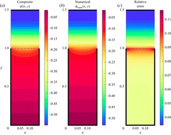


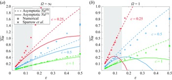


 Open access