


1. Introduction
The prediction of hydrodynamic forces acting on a body in relative motion to the surrounding fluid has tremendous practical relevance in a wide range of engineering applications. Oddly, even when the overall configuration is symmetric, the flow field may be asymmetric on long time scales despite the symmetry of the arrangement. Such asymmetric flow fields in symmetric configurations have been observed for diffusers, bumps, jets in cross-flow and wakes of both slender and bluff bodies, to mention a few examples. Despite its occurrence in a wide range of practically relevant problems, this phenomenon is not well understood (Williams & Smits Reference Williams and Smits2025).
The flow around the prolate spheroid has received a lot of attention because of its relevance to the maritime and aerospace industries, where asymmetry is of great importance to the loads. Asymmetry has been reported by several authors; however, its occurrence is not well understood. The object of this study is to comprehensively analyse the development of the asymmetry in the case of the flow around the spheroid.
The dynamics of the flow in the vicinity of the spheroid has been studied over a wide Reynolds number range. At very low Reynolds numbers ( $ \textit{Re}\lt 100$
), the flow around the spheroid has been investigated to obtain drag, lift and torque correlations which are useful for particle-laden flows (e.g. Fröhlich et al. (Reference Fröhlich, Meinke and Schröder2020)). In this Reynolds number regime, no asymmetry has been reported in the flow field. In the intermediate Reynolds numbers region (
$ \textit{Re}\lt 100$
), the flow around the spheroid has been investigated to obtain drag, lift and torque correlations which are useful for particle-laden flows (e.g. Fröhlich et al. (Reference Fröhlich, Meinke and Schröder2020)). In this Reynolds number regime, no asymmetry has been reported in the flow field. In the intermediate Reynolds numbers region ( $ \textit{Re} \approxeq \mathcal{O}(10^3{-}10^4)$
), several numerical studies have observed asymmetry in the flow field. In the range of
$ \textit{Re} \approxeq \mathcal{O}(10^3{-}10^4)$
), several numerical studies have observed asymmetry in the flow field. In the range of $ \textit{Re}\in [1000,8000]$
at an angle of attack of
$ \textit{Re}\in [1000,8000]$
at an angle of attack of $45^\circ$
, a series of studies utilising direct numerical simulation (DNS) (Jiang et al. Reference Jiang, Gallardo and Andersson2014, Reference Jiang, Gallardo, Andersson and Zhang2015, Reference Jiang, Andersson, Gallardo and Okulov2016; Strandenes et al. Reference Strandenes, Jiang, Pettersen and Andersson2019a
,
Reference Strandenes, Jiang, Pettersen and Anderssonb
; Andersson et al. Reference Andersson, Jiang and Okulov2019) observed and characterised the asymmetry of the counter-rotating vortex pair in the wake of the spheroid. However, no explanation for the emergence of the asymmetry was provided. In addition, Nidhan et al. (Reference Nidhan, Jain, Ortiz-Tarin and Sarkar2025) reported asymmetry in the wake of the spheroid at an angle of attack of
$45^\circ$
, a series of studies utilising direct numerical simulation (DNS) (Jiang et al. Reference Jiang, Gallardo and Andersson2014, Reference Jiang, Gallardo, Andersson and Zhang2015, Reference Jiang, Andersson, Gallardo and Okulov2016; Strandenes et al. Reference Strandenes, Jiang, Pettersen and Andersson2019a
,
Reference Strandenes, Jiang, Pettersen and Anderssonb
; Andersson et al. Reference Andersson, Jiang and Okulov2019) observed and characterised the asymmetry of the counter-rotating vortex pair in the wake of the spheroid. However, no explanation for the emergence of the asymmetry was provided. In addition, Nidhan et al. (Reference Nidhan, Jain, Ortiz-Tarin and Sarkar2025) reported asymmetry in the wake of the spheroid at an angle of attack of $10^\circ$
and
$10^\circ$
and $ \textit{Re}=30\,000$
(length-based
$ \textit{Re}=30\,000$
(length-based $ \textit{Re}$
) in their large eddy simulation (LES), when the Froude number was high (the stratification was weak).
$ \textit{Re}$
) in their large eddy simulation (LES), when the Froude number was high (the stratification was weak).
Ashok, Buren & Smits (Reference Ashok, Buren and Smits2015) investigated the DARPA SUBOFF experiments at angles of attack $\alpha \in [0,4,8,12]^\circ$
and
$\alpha \in [0,4,8,12]^\circ$
and $1.1\times 10^6\lt Re\lt 67\times 10^6$
. They documented an asymmetry in the flow field that was robust to variations in the pitch, yaw, trip wire geometry, level of free-stream turbulence and surface roughness; furthermore, the asymmetry was observed with two separate scale models in two different wind tunnels. The reason for the flow asymmetry was unknown.
$1.1\times 10^6\lt Re\lt 67\times 10^6$
. They documented an asymmetry in the flow field that was robust to variations in the pitch, yaw, trip wire geometry, level of free-stream turbulence and surface roughness; furthermore, the asymmetry was observed with two separate scale models in two different wind tunnels. The reason for the flow asymmetry was unknown.
Asymmetry of the flow field has been studied in configurations similar to the spheroid flow, such as cones, delta wings and cylinders with conical/ogive/hemisphere caps. In these flows, the side forces can be attributed to the asymmetry of the vortex pair that forms near the front of the body. Several important aspects have been described, such as the influence of the boundary layer state (laminar/transitional/turbulent) on the separation, and thus, the asymmetry (Lamont Reference Lamont1982), and scaling parameters have been proposed to characterise the asymmetry (Kumar, Viswanath & Ramesh Reference Kumar, Viswanath and Ramesh2005; Ma, Wang & Gursul Reference Ma, Wang and Gursul2017). The mechanism behind the asymmetry is not understood. As highlighted by Woolard (Reference Woolard1982), there are two main explanations for the emergence of the asymmetry. On the one hand, Keener & Chapman (Reference Keener and Chapman1977) suggested that asymmetry is driven by an inviscid vortex instability, which is related to the ‘crowdedness’ of the vortices. This is commonly referred to as the hydrodynamic instability argument. On the other hand, it has also been proposed that the asymmetry develops because of an asymmetry in the separation/reattachment of the flow (e.g. Ericsson (Reference Ericsson1992)). Another aspect of asymmetry in aerospace applications is the debate over whether it is due to a convective or a global instability (Huerre & Monkewitz Reference Huerre and Monkewitz1990). Earlier studies support the convective instability argument since they have established that even microscopic imperfections (that occur due to the limited precision of the manufacturing of the test piece) may trigger the asymmetry, and changing the roll angle of the model may induce significant variation in the side force coefficient (e.g. Moskovitz, Dejarnette & Hall (Reference Moskovitz, Dejarnette and Hall1989)).
A different class of flows that has received considerable attention regarding long-time-scale flow asymmetry is bluff body wakes – either bodies with axisymmetry (Rigas et al. Reference Rigas, Oxlade, Morgans and Morrison2014) or reflectional symmetry such as Ahmed bodies (Grandemange, Gohlke & Cadot Reference Grandemange, Gohlke and Cadot2013). It has been found that the stationary asymmetric flow structures that can be observed in the low $ \textit{Re}$
flow also appear at high
$ \textit{Re}$
flow also appear at high $ \textit{Re}$
in both the reflectionally symmetric (Grandemange et al. Reference Gómez, Gvmez and Theofilis2012, Reference Grandemange, Gohlke and Cadot2013) and axisymmetric cases (Rigas et al. Reference Rigas, Oxlade, Morgans and Morrison2014, Reference Rigas, Esclapez and Magri2016; Zhu, Rigas & Morrison Reference Zhu, Rigas and Morrison2025). Recently, a few studies have concentrated on the low Reynolds number stability analysis of bluff body wakes. Chiarini, Gauthier & Boujo (Reference Chiarini, Gauthier and Boujo2025) used global stability analysis to identify the active regions of the flow and confirm the stability criterion of the symmetry loss of axisymmetric wakes conjectured by Magnaudet & Mougin (Reference Magnaudet and Mougin2007). The criterion is based on the maxima of the azimuthal vorticity gradient: the instability originates from the azimuthal vorticity wanting to follow both the rigid body and the free stream, which creates large gradients.
$ \textit{Re}$
in both the reflectionally symmetric (Grandemange et al. Reference Gómez, Gvmez and Theofilis2012, Reference Grandemange, Gohlke and Cadot2013) and axisymmetric cases (Rigas et al. Reference Rigas, Oxlade, Morgans and Morrison2014, Reference Rigas, Esclapez and Magri2016; Zhu, Rigas & Morrison Reference Zhu, Rigas and Morrison2025). Recently, a few studies have concentrated on the low Reynolds number stability analysis of bluff body wakes. Chiarini, Gauthier & Boujo (Reference Chiarini, Gauthier and Boujo2025) used global stability analysis to identify the active regions of the flow and confirm the stability criterion of the symmetry loss of axisymmetric wakes conjectured by Magnaudet & Mougin (Reference Magnaudet and Mougin2007). The criterion is based on the maxima of the azimuthal vorticity gradient: the instability originates from the azimuthal vorticity wanting to follow both the rigid body and the free stream, which creates large gradients.
The usefulness of low $ \textit{Re}$
linear stability analysis in the case of bluff body wakes suggests that it may provide insight into the mechanism of flow asymmetries in other configurations. Tezuka & Suzuki (Reference Tezuka and Suzuki2006) conducted low Reynolds number stability analysis of a 4 : 1 prolate spheroid at zero and
$ \textit{Re}$
linear stability analysis in the case of bluff body wakes suggests that it may provide insight into the mechanism of flow asymmetries in other configurations. Tezuka & Suzuki (Reference Tezuka and Suzuki2006) conducted low Reynolds number stability analysis of a 4 : 1 prolate spheroid at zero and $\alpha =10^\circ$
angle of attack. They found that, in both cases, if the Reynolds number is sufficiently high, the flow becomes unstable to a stationary asymmetric eigenmode. Then, when the Reynolds number is further increased, the flow starts to produce an additional shedding mode. They noted that the structure of the asymmetric mode was the same in the two cases; however, they did not provide an explanation for why the asymmetry arises in the flow field.
$\alpha =10^\circ$
angle of attack. They found that, in both cases, if the Reynolds number is sufficiently high, the flow becomes unstable to a stationary asymmetric eigenmode. Then, when the Reynolds number is further increased, the flow starts to produce an additional shedding mode. They noted that the structure of the asymmetric mode was the same in the two cases; however, they did not provide an explanation for why the asymmetry arises in the flow field.
Thus, this work investigates the prolate 6 : 1 spheroid flow using global linear modal stability analysis for incompressible flow. The goal of the study is to find the first bifurcation and characterise the flow field to provide insight into the emergence of the asymmetry, and compare the trends with previous studies that reported an asymmetric flow field in similar flow configurations. The calculations are carried out using the open-source finite element library FreeFEM (Hecht Reference Hecht2012). First, starting from the sphere, the aspect ratio of the spheroid is progressively increased to six, and the stability of the flow is characterised. Then, the angle of attack of the 6 : 1 spheroid is varied between $0^\circ$
and
$0^\circ$
and $90^\circ$
.
$90^\circ$
.
The rest of this paper is organised as follows. Section 2 discusses the problem definition, modelling assumptions and the numerical solution techniques. Section 3 is concerned with varying the aspect ratio of the spheroid at zero angle of attack, and in § 4, the effect of angle of attack variation is presented on the stability of the flow around the 6 : 1 spheroid. The results are summarised in § 5.
2. Methodology
2.1. Problem set-up
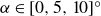
The flow configuration is illustrated in figure 1, where a rigid spheroid is placed in a uniform incompressible flow. The origin of the Cartesian coordinate system, in which the results are presented, is located at the centre of the spheroid. The $x$
axis is aligned with the major axis of the spheroid; a change in the angle of attack
$x$
axis is aligned with the major axis of the spheroid; a change in the angle of attack $\alpha$
corresponds to rotations around the
$\alpha$
corresponds to rotations around the $z$
axis; the normal coordinate
$z$
axis; the normal coordinate $y$
is perpendicular to the free stream at
$y$
is perpendicular to the free stream at $\alpha =0^\circ$
and aligned with it at
$\alpha =0^\circ$
and aligned with it at $\alpha =90^\circ$
. Some of the results are presented in a right-handed cylindrical coordinate system
$\alpha =90^\circ$
. Some of the results are presented in a right-handed cylindrical coordinate system $(x,r,\theta )$
, in which the axial direction is the same as in the Cartesian coordinate system. Dimensional quantities are denoted with a hat (
$(x,r,\theta )$
, in which the axial direction is the same as in the Cartesian coordinate system. Dimensional quantities are denoted with a hat ( $\hat {\square }$
), while non-dimensional quantities are denoted with regular letters. In the non-dimensionalisation of the equations, the velocity scale is the undisturbed free-stream velocity
$\hat {\square }$
), while non-dimensional quantities are denoted with regular letters. In the non-dimensionalisation of the equations, the velocity scale is the undisturbed free-stream velocity $\hat {U}_\infty$
, and the length scale is the diameter at the largest cross-section of the spheroid
$\hat {U}_\infty$
, and the length scale is the diameter at the largest cross-section of the spheroid $\hat {D}$
, which yields the following Reynolds number:
$\hat {D}$
, which yields the following Reynolds number:
 \begin{align} Re = \frac {\hat {D}\hat {U}_\infty }{\hat {\nu }}, \end{align}
where $\hat {\nu }$
is the kinematic viscosity of the fluid.
$\hat {\nu }$
is the kinematic viscosity of the fluid.
Sketch of the configuration.

2.2. Governing equations
Global modal linear stability analysis is utilised to characterise the stability of the flow. In this framework, the total velocity field is decomposed into a stationary equilibrium solution, called base flow, and a small-amplitude perturbation around the base flow, whose behaviour determines the stability of the flow. Let $\boldsymbol{U}=[U,V,W]^\intercal$
and
$\boldsymbol{U}=[U,V,W]^\intercal$
and $P$
denote the base flow velocity and pressure, and
$P$
denote the base flow velocity and pressure, and $\boldsymbol{u}'=[u',v',w']^\intercal$
and
$\boldsymbol{u}'=[u',v',w']^\intercal$
and $p'$
denote the velocity and pressure of the small-amplitude perturbations. Then, the non-dimensional governing equations of the base flow are
$p'$
denote the velocity and pressure of the small-amplitude perturbations. Then, the non-dimensional governing equations of the base flow are
 \begin{align} (\boldsymbol{U\boldsymbol{\cdot }\boldsymbol{\nabla }}) \boldsymbol{U} = -{\boldsymbol{\nabla }}P + \frac {1}{Re}{\boldsymbol{\nabla} }^2 \boldsymbol{U},\quad {\boldsymbol{\nabla }\boldsymbol{\cdot }\boldsymbol{U}} = 0. \end{align}
Once the stationary equilibrium base flow is obtained, its stability can be assessed using the linearised Navier–Stokes equations
 \begin{align} \frac {\partial \boldsymbol{u}'}{\partial t} + (\boldsymbol{U\boldsymbol{\cdot }\boldsymbol{\nabla }}) \boldsymbol{u}' + (\boldsymbol{u}'{\boldsymbol{\cdot }\boldsymbol{\nabla }}) \boldsymbol{U}= -{\boldsymbol{\nabla }}p' + \frac {1}{Re}{\boldsymbol{\nabla} }^2\boldsymbol{u}', \quad {\boldsymbol{\nabla }\boldsymbol{\cdot }\boldsymbol{u}}' = 0. \end{align}
Since the base flow is stationary, (2.3) can be further simplified by seeking the disturbances in the form
 \begin{align} \boldsymbol{q}'(x,y,z,t) = \boldsymbol{q}(x,y,z)e^{\sigma t} + \textrm{c.c}., \end{align}
where $ \boldsymbol{q} = [u,v,w,p]$
, the complex number
$ \boldsymbol{q} = [u,v,w,p]$
, the complex number $\sigma$
characterises the temporal variation of the disturbances and
$\sigma$
characterises the temporal variation of the disturbances and $\text{c.c.}$
stands for complex conjugate. The real part of
$\text{c.c.}$
stands for complex conjugate. The real part of $\sigma$
,
$\sigma$
, $\sigma _r$
, is the growth rate of the disturbances, and can be used to determine the stability of the flow: if it is positive, the flow is unstable, while negative values correspond to a stable flow. The imaginary part,
$\sigma _r$
, is the growth rate of the disturbances, and can be used to determine the stability of the flow: if it is positive, the flow is unstable, while negative values correspond to a stable flow. The imaginary part, $\sigma _i$
, is the angular frequency that characterises the oscillatory nature of the disturbances. Searching for the disturbances in this form, in essence, corresponds to utilising the Laplace transform, since the coefficients in the linearised Navier–Stokes equations are homogeneous in time. The ansatz (2.4) simplifies the solution of (2.3): the temporal variation is eliminated, but instead an eigenvalue problem needs to be solved, so the relevant flow structures can be computed directly. Typically, the least stable eigenvalues are sought at different Reynolds numbers, and the goal is to find the critical Reynolds number
$\sigma _i$
, is the angular frequency that characterises the oscillatory nature of the disturbances. Searching for the disturbances in this form, in essence, corresponds to utilising the Laplace transform, since the coefficients in the linearised Navier–Stokes equations are homogeneous in time. The ansatz (2.4) simplifies the solution of (2.3): the temporal variation is eliminated, but instead an eigenvalue problem needs to be solved, so the relevant flow structures can be computed directly. Typically, the least stable eigenvalues are sought at different Reynolds numbers, and the goal is to find the critical Reynolds number $ \textit{Re}_c$
, where the least stable eigenmode is marginally stable (
$ \textit{Re}_c$
, where the least stable eigenmode is marginally stable ( $\sigma _r=0$
), since this is where the disturbances reach only small amplitudes, and linear stability analysis can accurately predict the complete (nonlinear) flow field.
$\sigma _r=0$
), since this is where the disturbances reach only small amplitudes, and linear stability analysis can accurately predict the complete (nonlinear) flow field.
The disturbances in the form (2.4) can be obtained by solving the modal version of the linearised Navier–Stokes equations
 \begin{align} \sigma \boldsymbol{u} + (\boldsymbol{U\boldsymbol{\cdot }\boldsymbol{\nabla }}) \boldsymbol{u} + (\boldsymbol{u}{\boldsymbol{\cdot }\boldsymbol{\nabla }}) \boldsymbol{U}= -{\boldsymbol{\nabla }}p + \frac {1}{Re}{\boldsymbol{\nabla} }^2\boldsymbol{u},\quad {\boldsymbol{\nabla }\boldsymbol{\cdot }\boldsymbol{u}} = 0, \end{align}
which are also called TriGlobal stability equations (Theofilis Reference Theofilis2003). Equations (2.5) are complemented by their adjoint counterparts
 \begin{align} \sigma ^\dagger \boldsymbol{u}^\dagger + (\boldsymbol{U\boldsymbol{\cdot }\boldsymbol{\nabla }}) \boldsymbol{u}^\dagger + ({\boldsymbol{\nabla }} \boldsymbol{U}^\intercal ) \boldsymbol{u}^\dagger = -{\boldsymbol{\nabla }}p^\dagger - \frac {1}{Re}{\boldsymbol{\nabla} }^2\boldsymbol{u}^\dagger , \quad {\boldsymbol{\nabla }\boldsymbol{\cdot }\boldsymbol{u}}^\dagger = 0, \end{align}
where $\square ^\dagger$
denotes the adjoint quantities; note that
$\square ^\dagger$
denotes the adjoint quantities; note that $\sigma ^\dagger = \sigma ^*$
, where
$\sigma ^\dagger = \sigma ^*$
, where $\square ^*$
represents complex conjugation. The adjoint eigenmode that corresponds to the direct one characterises the receptivity of the direct mode to be excited by volumetric forcing in the domain or on the boundaries (Schmid & Henningson Reference Schmid and Henningson2001). In addition, the adjoint mode can be used to derive various sensitivity metrics (Marquet, Denis & Jacquin Reference Marquet, Denis and Jacquin2008; Fabre et al. Reference Fabre, Citro, Sabino, Bonnefis, Sierra, Giannetti and Pigou2019).
$\square ^*$
represents complex conjugation. The adjoint eigenmode that corresponds to the direct one characterises the receptivity of the direct mode to be excited by volumetric forcing in the domain or on the boundaries (Schmid & Henningson Reference Schmid and Henningson2001). In addition, the adjoint mode can be used to derive various sensitivity metrics (Marquet, Denis & Jacquin Reference Marquet, Denis and Jacquin2008; Fabre et al. Reference Fabre, Citro, Sabino, Bonnefis, Sierra, Giannetti and Pigou2019).
It is also convenient to write the modal version of the direct and adjoint linearised equations in the following form that clearly displays they correspond to linear eigenvalue problems:
 \begin{align} \sigma \boldsymbol{B} \boldsymbol{q} = \boldsymbol{A} \boldsymbol{q}, \quad \sigma ^\dagger \boldsymbol{B} \boldsymbol{q}^\dagger = \boldsymbol{A}^\dagger \boldsymbol{q}^\dagger . \end{align}
The elements of the matrices in the equation above are straightforward to derive. Note that $\boldsymbol{A}^\dagger = \boldsymbol{A}^{\mathsf{H}}$
, where
$\boldsymbol{A}^\dagger = \boldsymbol{A}^{\mathsf{H}}$
, where $\square ^{\mathsf{H}}$
denotes Hermitian (conjugate) transpose. Explicitly forming
$\square ^{\mathsf{H}}$
denotes Hermitian (conjugate) transpose. Explicitly forming $\boldsymbol{A}^\dagger$
in the discretisation process corresponds to the so-called continuous adjoint formulation, while forming
$\boldsymbol{A}^\dagger$
in the discretisation process corresponds to the so-called continuous adjoint formulation, while forming $\boldsymbol{A}$
first and using
$\boldsymbol{A}$
first and using $\boldsymbol{A}^\dagger = \boldsymbol{A}^{\mathsf{H}}$
is the discrete adjoint formulation. In principle, the two formulations are equivalent; in this study, the discrete adjoint method was used.
$\boldsymbol{A}^\dagger = \boldsymbol{A}^{\mathsf{H}}$
is the discrete adjoint formulation. In principle, the two formulations are equivalent; in this study, the discrete adjoint method was used.
In this work, the structural sensitivity (Giannetti & Luchini Reference Giannetti and Luchini2007) will also be used to characterise the important regions in the self-sustaining instability. The structural sensitivity $S$
is defined as follows:
$S$
is defined as follows:
 \begin{align} S(x,y,z) = |\boldsymbol{u}^{\dagger *} {\boldsymbol{\cdot }} \boldsymbol{u}|. \end{align}
The scalar field $S$
characterises the regions of the flow in which the local feedback is strong, and these regions are important in the development of the self-sustaining disturbance growth. The region of high structural sensitivity is often called the ‘wavemaker’ region, since it was first used to characterise the self-sustained flow oscillations in the wake of the flow behind a circular cylinder (Giannetti & Luchini Reference Giannetti and Luchini2007).
$S$
characterises the regions of the flow in which the local feedback is strong, and these regions are important in the development of the self-sustaining disturbance growth. The region of high structural sensitivity is often called the ‘wavemaker’ region, since it was first used to characterise the self-sustained flow oscillations in the wake of the flow behind a circular cylinder (Giannetti & Luchini Reference Giannetti and Luchini2007).
Using the standard inner product over the computational domain $\varOmega$
 \begin{align} \langle \boldsymbol{q}_1,\boldsymbol{q}_2 \rangle = \int _{\varOmega} \boldsymbol{u}_1^* \boldsymbol{\cdot }\boldsymbol{u}_2\, \mathrm{d}V, \end{align}
the direct and adjoint modes are normalised so that $\langle \boldsymbol{q},\boldsymbol{q} \rangle = 1$
and
$\langle \boldsymbol{q},\boldsymbol{q} \rangle = 1$
and $\langle \boldsymbol{q}^\dagger ,\boldsymbol{q} \rangle = 1$
. The normalisation
$\langle \boldsymbol{q}^\dagger ,\boldsymbol{q} \rangle = 1$
. The normalisation $\langle \boldsymbol{q}^\dagger ,\boldsymbol{q} \rangle = 1$
is convenient, since with a different normalisation of the adjoint mode, the term
$\langle \boldsymbol{q}^\dagger ,\boldsymbol{q} \rangle = 1$
is convenient, since with a different normalisation of the adjoint mode, the term $\langle \boldsymbol{q}^\dagger ,\boldsymbol{q} \rangle$
would appear in (2.8) (and also in (2.10), introduced later.)
$\langle \boldsymbol{q}^\dagger ,\boldsymbol{q} \rangle$
would appear in (2.8) (and also in (2.10), introduced later.)
The adjoint mode can also be used to determine the amplitude of the eigenmode triggered by a forcing with the same time dependency as the eigenmode. A detailed derivation of the amplitude equation for a parallel boundary layer is given by Hill (Reference Hill1995); here, only the results for the global stability problem are given. If (2.3) are forced on their right-hand sides with $\boldsymbol{f}'=[f_x(x,y,z),f_y(x,y,z),f_z(x,y,z)]^\intercal e^{\sigma _i t}$
and
$\boldsymbol{f}'=[f_x(x,y,z),f_y(x,y,z),f_z(x,y,z)]^\intercal e^{\sigma _i t}$
and $\varphi '=\varphi e^{\sigma _i t}$
, respectively, inside the domain without its boundaries (on
$\varphi '=\varphi e^{\sigma _i t}$
, respectively, inside the domain without its boundaries (on $\varOmega \setminus \partial \varOmega$
), then the amplitude of the mode (
$\varOmega \setminus \partial \varOmega$
), then the amplitude of the mode ( $a\boldsymbol{q}e^{\sigma t}$
) can be found as follows:
$a\boldsymbol{q}e^{\sigma t}$
) can be found as follows:
 \begin{align} a = \int _{\varOmega \setminus \partial \varOmega } \boldsymbol{u}^{\dagger *} {\boldsymbol{\cdot }} \boldsymbol{f} + p^{\dagger *} \varphi \,\mathrm{d}V. \end{align}
Equation (2.10) states that the adjoint mode can be used to weight the forcing to find the amplitude of the mode. It is important to state that (2.10) is only valid if the adjoint mode is normalised to the direct mode with (2.9). When inhomogeneous boundary conditions also force the disturbance mode, the adjoint stress and adjoint pressure can be used to evaluate the contribution from the boundary conditions to the amplitude, respectively. For more details regarding the rigorous derivation of the equations to find the mode amplitude, the interested reader is referred to Hill (Reference Hill1995).
2.3. Numerical method
The equations in the previous section are solved using computer programs developed in the open-source finite element package FreeFEM (Hecht Reference Hecht2012). The equations are discretised using Arnold–Brezzi–Fortin MINI-elements (first-order linear finite elements for both the velocity and pressure spaces; the elements for the velocity are augmented with a bubble function) on a tetrahedral mesh. For each configuration (aspect ratio and angle of attack), a separate unstructured tetrahedra mesh is created using the open-source software GMSH (Geuzaine & Remacle Reference Geuzaine and Remacle2009). Creating a separate mesh for each configuration is necessary to capture the structure of the wake region while keeping the size of the problem modest.
The equations are solved in a coordinate system $(\xi ,\eta ,\zeta )$
in which the
$(\xi ,\eta ,\zeta )$
in which the $\xi$
axis is aligned with the free stream, since this simplifies the specification of the boundary conditions; however, the results are presented in the coordinate system aligned with the spheroid. The rectangular computational domain, in which the spheroid is placed, is illustrated in figure 2. The centre of the spheroid is also the centre of the computational domain. The spheroid is placed symmetrically with respect to the computational domain in the
$\xi$
axis is aligned with the free stream, since this simplifies the specification of the boundary conditions; however, the results are presented in the coordinate system aligned with the spheroid. The rectangular computational domain, in which the spheroid is placed, is illustrated in figure 2. The centre of the spheroid is also the centre of the computational domain. The spheroid is placed symmetrically with respect to the computational domain in the $\eta$
and
$\eta$
and $\zeta$
directions; the sizes of the bounding box are detailed in table 1.
$\zeta$
directions; the sizes of the bounding box are detailed in table 1.
The size of the computational domain.

The computational domain. The coordinate systems $(\xi ,\eta ,\zeta )$
and
$(\xi ,\eta ,\zeta )$
and $(x,y,z)$
are aligned with the free stream and the spheroid, respectively.
$(x,y,z)$
are aligned with the free stream and the spheroid, respectively.

The boundary conditions are the following. At the inlet, the free-stream velocity is specified as the base flow ( $\boldsymbol{U}=[1, 0, 0]$
), and the perturbations are zero (
$\boldsymbol{U}=[1, 0, 0]$
), and the perturbations are zero ( $\boldsymbol{u}=\boldsymbol{u}^\dagger =0$
). At the wall of the spheroid, no-slip conditions are enforced for both the base flow and the perturbations (
$\boldsymbol{u}=\boldsymbol{u}^\dagger =0$
). At the wall of the spheroid, no-slip conditions are enforced for both the base flow and the perturbations ( $\boldsymbol{U}=\boldsymbol{u}'=\boldsymbol{u}^\dagger = [0,0,0]^\intercal$
). On the sidewall of the computational box, a free-slip boundary condition is prescribed (the normal velocity is zero, and the normal derivative of the tangential velocity components is zero). Finally, at the downstream end of the computational domain, a free-stress condition, which is automatically satisfied in the finite element formulation, constitutes the boundary condition.
$\boldsymbol{U}=\boldsymbol{u}'=\boldsymbol{u}^\dagger = [0,0,0]^\intercal$
). On the sidewall of the computational box, a free-slip boundary condition is prescribed (the normal velocity is zero, and the normal derivative of the tangential velocity components is zero). Finally, at the downstream end of the computational domain, a free-stress condition, which is automatically satisfied in the finite element formulation, constitutes the boundary condition.
The base flow is obtained using the Newton–Raphson technique, and the leading eigenvalues are found using the Krylov–Schur method. The implementations of these two methods in the PETSc (Balay et al. Reference Balay2021) and SLEPc (Roman et al. Reference Roman, Campos, Dalcin, Romero and Tomas2022) libraries are utilised in the computations. Both of these methods require the application of the inverse of the linearised Navier–Stokes operator, which is the most computationally intensive part of the solution procedure. The solution of linear systems of equations was obtained using LU factorisation with the MUMPS library (Amestoy et al. Reference Amestoy, Duff, L’Excellent and Koster2001). Special care was taken to tailor a mesh to each configuration (for each aspect ratio and angle of attack) to refine the mesh to the dynamically relevant flow regions.
As an illustration of the computational procedure, the mesh for the case with an angle of attack of $50^\circ$
is displayed in figure 3(a). In the plane
$50^\circ$
is displayed in figure 3(a). In the plane $z=0$
, the various mesh regions with different refinements can be clearly observed. The mesh is the finest near the spheroid; special attention was paid to resolve the near wake, while downstream of the body, the mesh becomes coarser. Also, the eigenspectrum obtained with the shift-invert method is presented in figure 3(b). The squares are the shifts, and the other symbols are the eigenvalues closest to the shifts. The dashed circles indicate the convergence radius of each shift-invert calculation. The regions of convergence overlap, so they cover the relevant part of the imaginary axis, so no eigenvalue is missed when it crosses the imaginary axis and becomes unstable.
$z=0$
, the various mesh regions with different refinements can be clearly observed. The mesh is the finest near the spheroid; special attention was paid to resolve the near wake, while downstream of the body, the mesh becomes coarser. Also, the eigenspectrum obtained with the shift-invert method is presented in figure 3(b). The squares are the shifts, and the other symbols are the eigenvalues closest to the shifts. The dashed circles indicate the convergence radius of each shift-invert calculation. The regions of convergence overlap, so they cover the relevant part of the imaginary axis, so no eigenvalue is missed when it crosses the imaginary axis and becomes unstable.
The calculations are performed on the Lighthouse cluster of the University of Michigan Advanced Research Computing. The simulations are run on 20 nodes, using 48 of the 192 processors per node. The FreeFEM and PETSc libraries were compiled using Intel compilers and MPI.
The base flow computations are conducted only on a domain halved at $z=0$
, where the symmetry of the base flow was enforced as a boundary condition. Then, the mesh and the base flow are mirrored for the stability calculations. This makes the base flow perfectly symmetric in the stability calculations at an angle of attack. Despite the large downstream extent of the computational domain in the downstream direction, flow structures may reach the downstream boundary and potentially hinder the convergence of the Newton–Raphson method. To circumvent convergence issues in the base flow calculations, the viscosity is artificially increased far downstream of the spheroid. The viscosity was varied, following Meliga, Gallaire & Chomaz (Reference Meliga, Gallaire and Chomaz2012) as
$z=0$
, where the symmetry of the base flow was enforced as a boundary condition. Then, the mesh and the base flow are mirrored for the stability calculations. This makes the base flow perfectly symmetric in the stability calculations at an angle of attack. Despite the large downstream extent of the computational domain in the downstream direction, flow structures may reach the downstream boundary and potentially hinder the convergence of the Newton–Raphson method. To circumvent convergence issues in the base flow calculations, the viscosity is artificially increased far downstream of the spheroid. The viscosity was varied, following Meliga, Gallaire & Chomaz (Reference Meliga, Gallaire and Chomaz2012) as
 \begin{align} \nu = \begin{cases} \nu _0 & \text{if $\xi \lt \xi _0$},\\ \nu _0 + (\nu _1-\nu _0) \boldsymbol{\cdot }\left ( 0.5 + 0.5 \tanh \left ( \tau \tan \left ( - \frac {\pi }{2} + \pi \boldsymbol{\cdot }\frac {\xi -\xi _0}{\xi _1-\xi _0} \right ) \right ) \right ) & \text{if $\xi _0\lt \xi \lt \xi _1$},\\ \nu _1 & \text{if $\xi \gt \xi _1$}, \end{cases} \end{align}
where $\nu _0=1/Re$
is the physical kinematic viscosity,
$\nu _0=1/Re$
is the physical kinematic viscosity, $\nu _1$
is the maximum value to which the viscosity is smoothly increased,
$\nu _1$
is the maximum value to which the viscosity is smoothly increased, $\xi _0$
and
$\xi _0$
and $\xi _1$
are the upstream and downstream ends of the region in which the viscosity varies and
$\xi _1$
are the upstream and downstream ends of the region in which the viscosity varies and $\tau$
influences the rate of the viscosity variation. The value of these parameters can be found in table 2.
$\tau$
influences the rate of the viscosity variation. The value of these parameters can be found in table 2.
The values the function that prescribes a spatially varying viscosity (2.11).

Illustrations of the numerical solution of the stability problem. (a) Mesh refinement near the spheroid and in its wake. Angle of attack is $50^\circ$
. (b) Eigenspectrum of the linearised Navier–Stokes equation calculated with the shift-invert method. Here,
$50^\circ$
. (b) Eigenspectrum of the linearised Navier–Stokes equation calculated with the shift-invert method. Here, $\alpha =90^\circ$
,
$\alpha =90^\circ$
, $ \textit{Re}_D=90$
.
$ \textit{Re}_D=90$
.

The numerical implementation of the modelling equations was verified by reproducing the results of previous studies. Good agreement was found in the leading eigenvalues for the plane channel flow at and the lid-driven cavity at $ \textit{Re}=1000$
with Giannetti, Luchini & Marino (Reference Giannetti, Luchini and Marino2009) and Juniper, Hanifi & Theofilis (Reference Juniper, Hanifi and Theofilis2014), Gómez et al. (Reference Gómez, Gvmez and Theofilis2014) and Regan & Mahesh (Reference Regan and Mahesh2017), respectively. The first two bifurcations in the case of the sphere were found at
$ \textit{Re}=1000$
with Giannetti, Luchini & Marino (Reference Giannetti, Luchini and Marino2009) and Juniper, Hanifi & Theofilis (Reference Juniper, Hanifi and Theofilis2014), Gómez et al. (Reference Gómez, Gvmez and Theofilis2014) and Regan & Mahesh (Reference Regan and Mahesh2017), respectively. The first two bifurcations in the case of the sphere were found at $ \textit{Re}=212.1$
and
$ \textit{Re}=212.1$
and $ \textit{Re}=280.1$
, consistent with Natarajan & Acrivos (Reference Natarajan and Acrivos1993), Meliga, Chomaz & Sipp (Reference Meliga, Chomaz and Sipp2009) and Citro et al. (Reference Citro, Tchoufag, Fabre, Giannetti and Luchini2016), while the growth rates of the stationary asymmetric mode of the 4 : 1 spheroid are in good agreement with Tezuka & Suzuki (Reference Tezuka and Suzuki2006).
$ \textit{Re}=280.1$
, consistent with Natarajan & Acrivos (Reference Natarajan and Acrivos1993), Meliga, Chomaz & Sipp (Reference Meliga, Chomaz and Sipp2009) and Citro et al. (Reference Citro, Tchoufag, Fabre, Giannetti and Luchini2016), while the growth rates of the stationary asymmetric mode of the 4 : 1 spheroid are in good agreement with Tezuka & Suzuki (Reference Tezuka and Suzuki2006).
3. Effect of varying the aspect ratio
The aspect ratio is varied between 1 (sphere) and 6 : 1 at zero angle of attack. The base flows are calculated at a wide range of Reynolds numbers, the relevant part of the eigenspectrum of the flow is calculated and the most unstable mode is identified. At each aspect ratio, there is a leading duplicate eigenvalue pair with zero frequency, which corresponds to the azimuthal wavenumber of one, in agreement with the previous investigation of axisymmetric bluff bodies (Rigas, Esclapez & Magri Reference Rigas, Esclapez and Magri2016). The reason for two eigenvalues instead of a single one is that the mesh is not axisymmetric (which would be the case if the problem was solved in a cylindrical coordinate system); it only possesses reflectional symmetry. The fact that the symmetry of the mesh does not obey the symmetry of the leading mode results in the eigenvalue breaking up into a pair.
The critical Reynolds number of the leading mode as a function of the aspect ratio is displayed in figure 4. As the aspect ratio increases and the body becomes more streamlined, the flow becomes unstable at higher and higher Reynolds numbers. It is worth mentioning that the present prediction of the critical Reynolds number in the case of the 4 : 1 spheroid matches with Tezuka & Suzuki (Reference Tezuka and Suzuki2006).
Critical Reynolds number of the leading eigenmode of the flow around the spheroid as a function of the aspect ratio at zero angle of attack.

The structure of the leading mode is illustrated by its axial velocity component in figure 5 for aspect ratios 1 : 1 (sphere), 2 : 1 and 4 : 1 (the 6 : 1 case is shown in figure 10 a). Each case is displayed close to the critical Reynolds number, where linear stability analysis is the most meaningful. The flow field is the same in all cases: the wake is deflected to one side, and has only a reflectional symmetry instead of the axisymmetry, where the reflectional symmetry axis may take any direction depending on the initial condition that triggered it. The similarity of the flow fields in figure 5 establishes that the same mechanism is behind the asymmetry of the flow at different aspect ratios.
The axial component of the leading eigenmode at $x=\textit{const.}$
cross-sections at different aspect ratios near the critical Reynolds number. (a) Sphere,
$x=\textit{const.}$
cross-sections at different aspect ratios near the critical Reynolds number. (a) Sphere, $ \textit{Re}_D=210$
; (b) 2 : 1 spheroid,
$ \textit{Re}_D=210$
; (b) 2 : 1 spheroid, $ \textit{Re}_D=400$
; (c) 4 : 1 spheroid,
$ \textit{Re}_D=400$
; (c) 4 : 1 spheroid, $ \textit{Re}_D=1000$
.
$ \textit{Re}_D=1000$
.

To characterise the base flow, the recirculation length $L_r$
is plotted in figure 6(a). As a verification of the computations, it is shown that in the case of the sphere, the values of
$L_r$
is plotted in figure 6(a). As a verification of the computations, it is shown that in the case of the sphere, the values of $L_r$
agree well with the ones obtained by Fornberg (Reference Fornberg1988) and Natarajan & Acrivos (Reference Natarajan and Acrivos1993) (
$L_r$
agree well with the ones obtained by Fornberg (Reference Fornberg1988) and Natarajan & Acrivos (Reference Natarajan and Acrivos1993) ( $\times$
and
$\times$
and $+$
symbols, respectively). It is apparent that increasing the aspect ratio corresponds to a more streamlined body with a weaker recirculation in its wake. Thus, since recirculation is crucial in the self-sustained global mode as it is responsible for the feedback of disturbances by convecting them upstream (Chomaz Reference Chomaz2005), the destabilisation of the flow at higher Reynolds numbers when the aspect ratio is increased may be attributed to a weaker recirculation.
$+$
symbols, respectively). It is apparent that increasing the aspect ratio corresponds to a more streamlined body with a weaker recirculation in its wake. Thus, since recirculation is crucial in the self-sustained global mode as it is responsible for the feedback of disturbances by convecting them upstream (Chomaz Reference Chomaz2005), the destabilisation of the flow at higher Reynolds numbers when the aspect ratio is increased may be attributed to a weaker recirculation.
Characterisation of the base flow around the spheroid for different aspect ratios at zero angle of attack. (a) Recirculation length in the wake of the spheroid with different aspect ratios as a function of $ \textit{Re}_D$
. In the legend, Fo. and N. & A. refer to the data of Fornberg (Reference Fornberg1988) and Natarajan & Acrivos (Reference Natarajan and Acrivos1993), respectively. (b) Drag correction factor
$ \textit{Re}_D$
. In the legend, Fo. and N. & A. refer to the data of Fornberg (Reference Fornberg1988) and Natarajan & Acrivos (Reference Natarajan and Acrivos1993), respectively. (b) Drag correction factor $F_d/F_{\textit{Stokes}}$
as a function of
$F_d/F_{\textit{Stokes}}$
as a function of $ \textit{Re}_D$
. In the legend, Fr. refers to the data of Fröhlich et al. (Reference Fröhlich, Meinke and Schröder2020).
$ \textit{Re}_D$
. In the legend, Fr. refers to the data of Fröhlich et al. (Reference Fröhlich, Meinke and Schröder2020).

Stability chart of the 6 : 1 spheroid as a function of the Reynolds number and the angle of attack. The dots denote parameter combinations at which the stability calculation was carried out. The black dots correspond to a stable flow; blue and red dots mark stationary asymmetric and oscillatory shedding modes, respectively. The $\times$
symbols mark the critical Reynolds number obtained using interpolation. (a) complete parameter space. The regions
$\times$
symbols mark the critical Reynolds number obtained using interpolation. (a) complete parameter space. The regions $[64{-}73]^\circ$
and
$[64{-}73]^\circ$
and $[44{-}52]^\circ$
, which are marked with the boxes in subfigure (a), are displayed in subfigures (b) and (c), respectively.
$[44{-}52]^\circ$
, which are marked with the boxes in subfigure (a), are displayed in subfigures (b) and (c), respectively.

In figure 6(b) the drag correction factor $F_d/F_{\textit{Stokes}}$
is presented. In the ratio
$F_d/F_{\textit{Stokes}}$
is presented. In the ratio $F_d/F_{\textit{Stokes}}$
,
$F_d/F_{\textit{Stokes}}$
, $F_d$
is the drag force obtained from the simulation, and
$F_d$
is the drag force obtained from the simulation, and $F_{\textit{Stokes}}$
is the drag force in Stokes flow (which can be calculated in closed form, see (Happel & Brenner Reference Happel and Brenner1983, § 4.30)). As the aspect ratio is increased, the drag surplus caused by finite Reynolds number effects becomes slightly less important. It is noted that the
$F_{\textit{Stokes}}$
is the drag force in Stokes flow (which can be calculated in closed form, see (Happel & Brenner Reference Happel and Brenner1983, § 4.30)). As the aspect ratio is increased, the drag surplus caused by finite Reynolds number effects becomes slightly less important. It is noted that the $F_d/F_{\textit{Stokes}}$
values agree well with the calculations of Fröhlich et al. (Reference Fröhlich, Meinke and Schröder2020).
$F_d/F_{\textit{Stokes}}$
values agree well with the calculations of Fröhlich et al. (Reference Fröhlich, Meinke and Schröder2020).
4. Angle of attack effects
4.1. Regime map
For the 6 : 1 spheroid, the main objective of the present work is to find the first bifurcation of the flow at every angle of attack to construct a stability chart as a function of $ \textit{Re}$
and
$ \textit{Re}$
and $\alpha$
, and then characterise the eigenmodes and the base flow. The stability chart is presented in figure 7(a) in the
$\alpha$
, and then characterise the eigenmodes and the base flow. The stability chart is presented in figure 7(a) in the $ \textit{Re}-\alpha$
plane. The black dots denote where the base flow is stable; the blue and red dots correspond to stationary asymmetric and oscillatory shedding modes, respectively; the
$ \textit{Re}-\alpha$
plane. The black dots denote where the base flow is stable; the blue and red dots correspond to stationary asymmetric and oscillatory shedding modes, respectively; the $\times$
symbols mark the marginally stable states, which are approximated by interpolating the growth rate and finding
$\times$
symbols mark the marginally stable states, which are approximated by interpolating the growth rate and finding $\sigma _r=0$
. For the sake of completeness, abscissas with both
$\sigma _r=0$
. For the sake of completeness, abscissas with both $ \textit{Re}_D$
and
$ \textit{Re}_D$
and $ \textit{Re}_L$
are presented, and critical Reynolds number values are tabulated in tables 3 and 4 for the stationary asymmetric and oscillatory shedding modes, respectively. There are two
$ \textit{Re}_L$
are presented, and critical Reynolds number values are tabulated in tables 3 and 4 for the stationary asymmetric and oscillatory shedding modes, respectively. There are two $\alpha$
intervals in which rapid changes can be observed in the trends of the stability characteristics of the flow. The two regions with
$\alpha$
intervals in which rapid changes can be observed in the trends of the stability characteristics of the flow. The two regions with $\alpha \in [45{-}50]^\circ$
and
$\alpha \in [45{-}50]^\circ$
and $\alpha \in [65{-}72]^\circ$
, are displayed separately in figures 7(c) and 7(b), respectively.
$\alpha \in [65{-}72]^\circ$
, are displayed separately in figures 7(c) and 7(b), respectively.
Critical Reynolds number of the first bifurcation of the spheroid flow at various angles of attack. Stationary asymmetric mode.

Critical Reynolds number of the first bifurcation of the spheroid flow at various angles of attack. Oscillatory shedding mode.

Several interesting observations can be made from figure 7. As the angle of attack is increased from zero, the critical Reynolds number of the stationary asymmetric leading mode continuously decreases until it reaches $25^\circ$
; then, it stays around
$25^\circ$
; then, it stays around $ \textit{Re}_D \approxeq 950$
in the interval
$ \textit{Re}_D \approxeq 950$
in the interval $\alpha \in [25{-}45]^\circ$
. When the angle of attack is increased from
$\alpha \in [25{-}45]^\circ$
. When the angle of attack is increased from $\alpha =45^\circ$
to
$\alpha =45^\circ$
to $\alpha =50^\circ$
, the critical Reynolds number decreases drastically; therefore, additional calculations were performed in this
$\alpha =50^\circ$
, the critical Reynolds number decreases drastically; therefore, additional calculations were performed in this $\alpha$
interval, which are displayed in figure 7(c). When the angle of attack is increased beyond
$\alpha$
interval, which are displayed in figure 7(c). When the angle of attack is increased beyond $\alpha =47^\circ$
, initially the change in the critical Reynolds number is slow, but then there is a large drop in
$\alpha =47^\circ$
, initially the change in the critical Reynolds number is slow, but then there is a large drop in $ \textit{Re}_c$
when moving from
$ \textit{Re}_c$
when moving from $\alpha =49.25^\circ$
to
$\alpha =49.25^\circ$
to $\alpha =49.5^\circ$
. In all the cases, the leading eigenmode is a stationary asymmetric one. Moving toward higher angle of attack values, the
$\alpha =49.5^\circ$
. In all the cases, the leading eigenmode is a stationary asymmetric one. Moving toward higher angle of attack values, the $ \textit{Re}_c$
value of the leading stationary asymmetric mode continues to decrease. The decline of
$ \textit{Re}_c$
value of the leading stationary asymmetric mode continues to decrease. The decline of $ \textit{Re}_c$
with an increase in
$ \textit{Re}_c$
with an increase in $\alpha$
only changes in the
$\alpha$
only changes in the $\alpha \in [65{-}70]^\circ$
region, which is shown in figure 7(b). Contrary to the previous trend, the critical Reynolds number of the stationary mode starts to increase with the angle of attack. The next angle of attack at which substantial changes occur is
$\alpha \in [65{-}70]^\circ$
region, which is shown in figure 7(b). Contrary to the previous trend, the critical Reynolds number of the stationary mode starts to increase with the angle of attack. The next angle of attack at which substantial changes occur is $\alpha =70^\circ$
: this is the last
$\alpha =70^\circ$
: this is the last $\alpha$
value at which the stationary asymmetric mode loses its stability, and for higher
$\alpha$
value at which the stationary asymmetric mode loses its stability, and for higher $\alpha$
, the leading eigenmode remains an oscillatory shedding mode. Finally, increasing the angle of attack past
$\alpha$
, the leading eigenmode remains an oscillatory shedding mode. Finally, increasing the angle of attack past $80^\circ$
does not influence the critical Reynolds number of the leading oscillatory shedding mode in a meaningful manner: its value stays around
$80^\circ$
does not influence the critical Reynolds number of the leading oscillatory shedding mode in a meaningful manner: its value stays around $ \textit{Re}_D \approxeq 90$
.
$ \textit{Re}_D \approxeq 90$
.
The calculated critical $ \textit{Re}$
values match the observations of previous studies. In the case of a 6 : 1 spheroid at an angle of attack of
$ \textit{Re}$
values match the observations of previous studies. In the case of a 6 : 1 spheroid at an angle of attack of $45^\circ$
, Andersson et al. (Reference Andersson, Jiang and Okulov2019) reported that in the DNS, the flow around the spheroid was perfectly symmetric at
$45^\circ$
, Andersson et al. (Reference Andersson, Jiang and Okulov2019) reported that in the DNS, the flow around the spheroid was perfectly symmetric at $ \textit{Re}_D=800$
, while at
$ \textit{Re}_D=800$
, while at $ \textit{Re}_D=1000$
a modest asymmetry was observed, meaning that the asymmetry in the flow field could be discerned only starting from
$ \textit{Re}_D=1000$
a modest asymmetry was observed, meaning that the asymmetry in the flow field could be discerned only starting from $x/D=8$
downstream of the spheroid (the origin of their coordinate system is at the centre of the spheroid, and the
$x/D=8$
downstream of the spheroid (the origin of their coordinate system is at the centre of the spheroid, and the $x$
direction aligns with the undisturbed free stream). The fact that the asymmetry they observed was weak means that their simulation is close to the neutrally stable Reynolds number and that the bifurcation is supercritical, which is consistent with the present prediction of
$x$
direction aligns with the undisturbed free stream). The fact that the asymmetry they observed was weak means that their simulation is close to the neutrally stable Reynolds number and that the bifurcation is supercritical, which is consistent with the present prediction of $ \textit{Re}_D=972.4$
.
$ \textit{Re}_D=972.4$
.
In the case of the $90^\circ$
spheroid, Khoury, Andersson & Pettersen (Reference Khoury, Andersson and Pettersen2012) performed DNS at low
$90^\circ$
spheroid, Khoury, Andersson & Pettersen (Reference Khoury, Andersson and Pettersen2012) performed DNS at low $ \textit{Re}$
values. They reported a symmetric flow field at
$ \textit{Re}$
values. They reported a symmetric flow field at $ \textit{Re}_D=75$
while at
$ \textit{Re}_D=75$
while at $ \textit{Re}_D=100$
the flow field was oscillatory, which accords with our prediction of the bifurcation at
$ \textit{Re}_D=100$
the flow field was oscillatory, which accords with our prediction of the bifurcation at $ \textit{Re}_D=86.7$
. Nidhan et al. (Reference Nidhan, Jain, Ortiz-Tarin and Sarkar2025) found using LES that at
$ \textit{Re}_D=86.7$
. Nidhan et al. (Reference Nidhan, Jain, Ortiz-Tarin and Sarkar2025) found using LES that at $\alpha =10^\circ$
and
$\alpha =10^\circ$
and $ \textit{Re}_D=5000$
(
$ \textit{Re}_D=5000$
( $ \textit{Re}_L=30\,000$
in their paper) the mean flow field was asymmetric, which is also consistent with predictions of the stability analysis.
$ \textit{Re}_L=30\,000$
in their paper) the mean flow field was asymmetric, which is also consistent with predictions of the stability analysis.
4.2. Low angle of attack
4.2.1. Skin friction lines
The skin friction lines are presented in figure 8 for angles of attack $\alpha \in [0,5,10]^\circ$
. The
$\alpha \in [0,5,10]^\circ$
. The $x$
axis is the axial direction, while on the
$x$
axis is the axial direction, while on the $y$
axis, the azimuthal angle
$y$
axis, the azimuthal angle $\varphi$
is presented; since the base flow is symmetric, only the
$\varphi$
is presented; since the base flow is symmetric, only the $\varphi \in [0,\pi ]$
interval is displayed. At zero angle of attack (figure 8
a), a circular separation line can be seen at an
$\varphi \in [0,\pi ]$
interval is displayed. At zero angle of attack (figure 8
a), a circular separation line can be seen at an $x=\textit{const.}$
location, from which the separating flow reattaches at the aft of the spheroid, forming the recirculating wake in the close downstream vicinity of the spheroid. At
$x=\textit{const.}$
location, from which the separating flow reattaches at the aft of the spheroid, forming the recirculating wake in the close downstream vicinity of the spheroid. At $\alpha =5^\circ$
, the topology of the flow separation changes compared with the zero angle of attack case, which is apparent by examining the skin friction lines that are shown in figure 8(b). The separation line is split into two parts at the two sides of the spheroid, which are fed mainly by the upstream flow, but it is also connected to the recirculation of the wake. The two separation lines at the two sides of the spheroid are connected at
$\alpha =5^\circ$
, the topology of the flow separation changes compared with the zero angle of attack case, which is apparent by examining the skin friction lines that are shown in figure 8(b). The separation line is split into two parts at the two sides of the spheroid, which are fed mainly by the upstream flow, but it is also connected to the recirculation of the wake. The two separation lines at the two sides of the spheroid are connected at $\varphi =\pi$
by the saddle point being their unstable directions, and the stable directions of the saddle point are the upstream inflow and the wake reverse flow.
$\varphi =\pi$
by the saddle point being their unstable directions, and the stable directions of the saddle point are the upstream inflow and the wake reverse flow.
Skin friction lines of the base flow. The 6 : 1 spheroid at low angles of attack near the critical Reynolds number: (a) $\alpha =0^\circ$
,
$\alpha =0^\circ$
, $ \textit{Re}_D=1800$
; (b)
$ \textit{Re}_D=1800$
; (b) $\alpha =5^\circ$
,
$\alpha =5^\circ$
, $ \textit{Re}_D=1550$
; (c)
$ \textit{Re}_D=1550$
; (c) $\alpha =10^\circ$
,
$\alpha =10^\circ$
, $ \textit{Re}_D=1300$
.
$ \textit{Re}_D=1300$
.

When the angle of attack is increased to $\alpha =10^\circ$
(figure 8
c), substantial changes can be observed in the skin friction lines. Although the saddle point at
$\alpha =10^\circ$
(figure 8
c), substantial changes can be observed in the skin friction lines. Although the saddle point at $\varphi =\pi$
, the separation line that connects the upstream inflow with the reverse flow at the trailing edge can all be identified as at
$\varphi =\pi$
, the separation line that connects the upstream inflow with the reverse flow at the trailing edge can all be identified as at $\alpha =5^\circ$
, two new flow features emerge. Below the saddle point at
$\alpha =5^\circ$
, two new flow features emerge. Below the saddle point at $\varphi =\pi$
, a stable focus can be identified, which corresponds to a specific flow separation that may only arise in three-dimensional flows. This type of separation has previously been observed in the experimental investigation of 2 : 1, 3 : 1 and 4 : 1 aspect ratio spheroids by Wang et al. (Reference Wang, Zhou, Hu, Harrington and Lighthill1990). In addition, a new saddle point can also be observed, that forms a boundary between the stable focus and the main separation line. Comparison of the skin friction lines at the three
$\varphi =\pi$
, a stable focus can be identified, which corresponds to a specific flow separation that may only arise in three-dimensional flows. This type of separation has previously been observed in the experimental investigation of 2 : 1, 3 : 1 and 4 : 1 aspect ratio spheroids by Wang et al. (Reference Wang, Zhou, Hu, Harrington and Lighthill1990). In addition, a new saddle point can also be observed, that forms a boundary between the stable focus and the main separation line. Comparison of the skin friction lines at the three $\alpha$
values clearly shows that the flow field changes significantly as the angle of attack is varied.
$\alpha$
values clearly shows that the flow field changes significantly as the angle of attack is varied.
4.2.2. Axial component of the base flow
The axial component of the base flow is presented at several axial stations in figure 9. The zero angle of attack case, displayed in figure 9(a) is, as expected, axisymmetric. When the angle of attack is increased to $\alpha =5^\circ$
(figure 9
b), the wake of the body initially looks like an axisymmetric bluff body wake; however, further downstream, the two counter-rotating vortices emerging from the separating flow can be clearly distinguished. Further increasing the angle of attack to
$\alpha =5^\circ$
(figure 9
b), the wake of the body initially looks like an axisymmetric bluff body wake; however, further downstream, the two counter-rotating vortices emerging from the separating flow can be clearly distinguished. Further increasing the angle of attack to $\alpha =10^\circ$
, the vortices become more pronounced compared with the
$\alpha =10^\circ$
, the vortices become more pronounced compared with the $\alpha =5^\circ$
case. The separation from the focus cannot be distinguished in the axial component of the base flow.
$\alpha =5^\circ$
case. The separation from the focus cannot be distinguished in the axial component of the base flow.
The axial component of the base flow around the 6 : 1 spheroid at $x=\textit{const.}$
cross-sections near the critical Reynolds number at low angles of attack: (a)
$x=\textit{const.}$
cross-sections near the critical Reynolds number at low angles of attack: (a) $\alpha =0^\circ$
,
$\alpha =0^\circ$
, $ \textit{Re}_D=1800$
; (b)
$ \textit{Re}_D=1800$
; (b) $\alpha =5^\circ$
,
$\alpha =5^\circ$
, $ \textit{Re}_D=1550$
; (c)
$ \textit{Re}_D=1550$
; (c) $\alpha =10^\circ$
,
$\alpha =10^\circ$
, $ \textit{Re}_D=1300$
.
$ \textit{Re}_D=1300$
.

4.2.3. Axial component of the asymmetric eigenmode
The axial component of the leading asymmetric eigenmode is presented at successive axial stations in figure 10. At zero angle of attack (figure 10
a), the same mode can be observed as in the lower aspect ratios presented in figure 5. As the angle of attack is increased to $\alpha =5^\circ$
and
$\alpha =5^\circ$
and $\alpha =10^\circ$
(figures 10
b and 10
c, respectively), the eigenmode is characterised by the same two patches of positive and negative velocity, similarly to
$\alpha =10^\circ$
(figures 10
b and 10
c, respectively), the eigenmode is characterised by the same two patches of positive and negative velocity, similarly to $\alpha =0^\circ$
. However, the emergence of the counter-rotating vortex pair at these angles of attack clearly changes the structure of the perturbation. At
$\alpha =0^\circ$
. However, the emergence of the counter-rotating vortex pair at these angles of attack clearly changes the structure of the perturbation. At $\alpha =10^\circ$
, two main patches are complemented by smaller regions of velocity below them whose sign is the opposite. Simultaneous examination of the figures clearly shows that the structure of the eigenmode changes continuously with the variation of the angle of attack, indicating that the same mechanism governs the asymmetry across all the cases.
$\alpha =10^\circ$
, two main patches are complemented by smaller regions of velocity below them whose sign is the opposite. Simultaneous examination of the figures clearly shows that the structure of the eigenmode changes continuously with the variation of the angle of attack, indicating that the same mechanism governs the asymmetry across all the cases.
The axial component of the leading eigenmode at $x=\textit{const.}$
cross-sections near the critical Reynolds number at low angles of attack: (a)
$x=\textit{const.}$
cross-sections near the critical Reynolds number at low angles of attack: (a) $\alpha =0^\circ$
,
$\alpha =0^\circ$
, $ \textit{Re}_D=1800$
; (b)
$ \textit{Re}_D=1800$
; (b) $\alpha =5^\circ$
,
$\alpha =5^\circ$
, $ \textit{Re}_D=1550$
; (c)
$ \textit{Re}_D=1550$
; (c) $\alpha =10^\circ$
,
$\alpha =10^\circ$
, $ \textit{Re}_D=1300$
.
$ \textit{Re}_D=1300$
.

4.2.4. Comparison with the experiments of Ashok et al. (Reference Ashok, Buren and Smits2015)
Studies of axisymmetric wakes (Rigas et al. Reference Rigas, Oxlade, Morgans and Morrison2014; Zhu et al. Reference Zhu, Rigas and Morrison2025) show that, in high Reynolds number flow, the dominant flow structures extracted using modal decomposition are qualitatively similar to the modes obtained from linear stability analysis. In order to compare the eigenmodes with an experimentally measured asymmetric mean flow of Ashok (Reference Ashok2014), the axial component of the base flow plus the asymmetric mode with an arbitrary amplitude chosen to visualise the flow is presented in figure 11. The total flow field resembles the well-documented vortex asymmetry of slender body flows, in which one vortex becomes stronger and ‘overcomes’ the other. The asymmetric mean flow field measured by Ashok (Reference Ashok2014) in their high Reynolds number DARPA SUBOFF experiments is displayed in figure 12. Despite the three orders of magnitude in the Reynolds number, and the geometric differences in the configuration (different geometry, difference in the angle of attack, blockage effects in the experiments and arbitrary amplitude of the perturbation added to the base flow), the qualitative similarity between the flow fields is striking. The qualitative agreement suggests that the stationary asymmetric mode was triggered in the experiments by some kind of imperfection.
The axial component of the base flow plus the leading eigenmode at $x=\textit{const.}$
cross-sections near the critical Reynolds number.
$x=\textit{const.}$
cross-sections near the critical Reynolds number. $\alpha =5^\circ$
,
$\alpha =5^\circ$
, $ \textit{Re}_D=1550$
.
$ \textit{Re}_D=1550$
.

Mean streamwise velocity component at $x/D=8$
, measured from the trailing edge of the DARPA SUBOFF model. Here,
$x/D=8$
, measured from the trailing edge of the DARPA SUBOFF model. Here, $ \textit{Re}_L = 2.4\times 10^6$
. Panels show (a)
$ \textit{Re}_L = 2.4\times 10^6$
. Panels show (a) $\alpha =2^\circ$
; (b)
$\alpha =2^\circ$
; (b) $\alpha =4^\circ$
; (c)
$\alpha =4^\circ$
; (c) $\alpha =8^\circ$
; (d)
$\alpha =8^\circ$
; (d) $\alpha =-2^\circ$
; (e)
$\alpha =-2^\circ$
; (e) $\alpha =-4^\circ$
; (f)
$\alpha =-4^\circ$
; (f) $\alpha =-8^\circ$
. Reproduced with permission.
$\alpha =-8^\circ$
. Reproduced with permission.

Flow field in the $y{-}z$
plane at
$y{-}z$
plane at $x/D=8$
(measured from the trailing edge) in the DARPA SUBOFF experiments of Ashok et al. (Reference Ashok, Buren and Smits2015). (a) Contour plot of the mean axial velocity; (b) contour plot of the mean in-plane velocity. In both figures, arrows illustrate the in-plane flow. Reproduced with permission of Cambridge University Press.
$x/D=8$
(measured from the trailing edge) in the DARPA SUBOFF experiments of Ashok et al. (Reference Ashok, Buren and Smits2015). (a) Contour plot of the mean axial velocity; (b) contour plot of the mean in-plane velocity. In both figures, arrows illustrate the in-plane flow. Reproduced with permission of Cambridge University Press.

The asymmetry was quite robust to changes in the parameters such as the pitch, yaw and trip geometry, and Ashok et al. (Reference Ashok, Buren and Smits2015) did not provide an explanation for the emergence of the asymmetry in the flow field. However, a possible reason for the asymmetry is the weak cross-plane flow, which is presented in figure 13. The orientation of the cross-plane flow compared with the model is preferential in one direction. As discussed in § 2.2, the adjoint mode complementing the direct mode can be used to determine the amplitude of the mode for a specific forcing (2.10). The spanwise component of the adjoint mode, which is relevant to the side flow in the experiments, is presented in figure 14. The characteristics of the adjoint mode are qualitatively similar in all cases. The adjoint modes have the largest amplitudes near the trailing edge in the close vicinity of the spheroid their amplitude is negligible near $x/L=1.167$
, and the spatial structure of the modes is also similar. However, the shape of the adjoint mode becomes more complicated as the angle of attack is increased.
$x/L=1.167$
, and the spatial structure of the modes is also similar. However, the shape of the adjoint mode becomes more complicated as the angle of attack is increased.
The structure of the spanwise component of the adjoint modes suggests that a forcing in the $z$
direction can trigger the mode. To provide quantitative evidence that the direct mode can be triggered by the side flow, the amplitude of the mode is evaluated with a forcing that mimics the side flow in the experiments and the adjoint mode. Since the side flow in the experiments is oriented in the
$z$
direction can trigger the mode. To provide quantitative evidence that the direct mode can be triggered by the side flow, the amplitude of the mode is evaluated with a forcing that mimics the side flow in the experiments and the adjoint mode. Since the side flow in the experiments is oriented in the $z$
direction, and it is given only at a specific axial station, the following forcing is prescribed:
$z$
direction, and it is given only at a specific axial station, the following forcing is prescribed:
 \begin{align} \boldsymbol{f} = \left [0,0,\delta (x_0)\right ]^\intercal , \end{align}
where $\delta (x_0)$
is the Dirac–delta function. (4.1) states that the forcing is only considered at a specific axial station. The amplitudes evaluated using (2.10) and (4.1), with the forcing localised at
$\delta (x_0)$
is the Dirac–delta function. (4.1) states that the forcing is only considered at a specific axial station. The amplitudes evaluated using (2.10) and (4.1), with the forcing localised at $x_0/L=1$
(the trailing edge of the spheroid), are displayed in table 5. For all three angles of attack considered, the forcing yields a non-zero amplitude, clearly showing that the mode can be triggered by a side flow. Thus, we formulate the conjecture that in the experiments of Ashok (Reference Ashok2014) and Ashok et al. (Reference Ashok, Buren and Smits2015), the side flow is responsible for the asymmetry. An additional detail that supports this conjecture is that the orientation of the mode depended on the sign of the pitch in the experiments, which is apparent in figure 12. Changing the pitch means a relative change in the direction of the side force compared with the DARPA SUBOFF model, which would change the orientation of the mode.
$x_0/L=1$
(the trailing edge of the spheroid), are displayed in table 5. For all three angles of attack considered, the forcing yields a non-zero amplitude, clearly showing that the mode can be triggered by a side flow. Thus, we formulate the conjecture that in the experiments of Ashok (Reference Ashok2014) and Ashok et al. (Reference Ashok, Buren and Smits2015), the side flow is responsible for the asymmetry. An additional detail that supports this conjecture is that the orientation of the mode depended on the sign of the pitch in the experiments, which is apparent in figure 12. Changing the pitch means a relative change in the direction of the side force compared with the DARPA SUBOFF model, which would change the orientation of the mode.


The spanwise ( $z$
) component of the leading adjoint eigenmode at
$z$
) component of the leading adjoint eigenmode at $x=\textit{const.}$
cross-sections near the critical Reynolds number at low angles of attack. Panels show (a)
$x=\textit{const.}$
cross-sections near the critical Reynolds number at low angles of attack. Panels show (a) $\alpha =0^\circ$
,
$\alpha =0^\circ$
, $ \textit{Re}_D=1800$
; (b)
$ \textit{Re}_D=1800$
; (b) $\alpha =5^\circ$
,
$\alpha =5^\circ$
, $ \textit{Re}_D=1550$
; (c)
$ \textit{Re}_D=1550$
; (c) $\alpha =10^\circ$
,
$\alpha =10^\circ$
, $ \textit{Re}_D=1300$
.
$ \textit{Re}_D=1300$
.

4.2.5. Structural sensitivity and the base flow vorticity
In the case of axisymmetric bodies, Chiarini et al. (Reference Chiarini, Gauthier and Boujo2025) have shown that the development of the asymmetric stationary instability is related to the gradients in the vorticity – because of the axisymmetry of their configurations, the azimuthal vorticity component. Thus, concluding the discussion of the low $\alpha$
regime, the vorticity fields and the structural sensitivity are analysed to shed light on the development of the instability mechanism. Only the azimuthal component of the vorticity (
$\alpha$
regime, the vorticity fields and the structural sensitivity are analysed to shed light on the development of the instability mechanism. Only the azimuthal component of the vorticity ( $\omega _\theta$
) is presented in figure 15 for the sake of brevity. The solid black contours show the isocontours of the structural sensitivity of the leading mode, which is the region of the flow that drives the instability. The
$\omega _\theta$
) is presented in figure 15 for the sake of brevity. The solid black contours show the isocontours of the structural sensitivity of the leading mode, which is the region of the flow that drives the instability. The $y=\textit{const.}$
locations are chosen so that areas with high values of structural sensitivity are shown.
$y=\textit{const.}$
locations are chosen so that areas with high values of structural sensitivity are shown.
Azimuthal vorticity of the base flow at $y=\textit{const.}$
cross-sections. The black contours show the structural sensitivity of the leading mode near the critical Reynolds number. Panels show (a)
$y=\textit{const.}$
cross-sections. The black contours show the structural sensitivity of the leading mode near the critical Reynolds number. Panels show (a) $\alpha =0^\circ$
,
$\alpha =0^\circ$
, $ \textit{Re}_D=1800$
; (b)
$ \textit{Re}_D=1800$
; (b) $\alpha =5^\circ$
,
$\alpha =5^\circ$
, $ \textit{Re}_D=1550$
; (c)
$ \textit{Re}_D=1550$
; (c) $\alpha =10^\circ$
,
$\alpha =10^\circ$
, $ \textit{Re}_D=1300$
.
$ \textit{Re}_D=1300$
.

Since the angle of attack is low, the evolution of the flow can be interpreted by examining the changes in the axial direction. In the case of $\alpha =0^\circ$
(figure 15
a), as pointed out by Chiarini et al. (Reference Chiarini, Gauthier and Boujo2025), the instability is driven by the strong gradients in the azimuthal vorticity near the recirculation bubble. The region of high structural sensitivity is aligned with the gradients in the azimuthal vorticity: it is located near the trailing edge of the spheroid, which overlaps with the region where
$\alpha =0^\circ$
(figure 15
a), as pointed out by Chiarini et al. (Reference Chiarini, Gauthier and Boujo2025), the instability is driven by the strong gradients in the azimuthal vorticity near the recirculation bubble. The region of high structural sensitivity is aligned with the gradients in the azimuthal vorticity: it is located near the trailing edge of the spheroid, which overlaps with the region where $\omega _\theta$
varies from negligible values (around
$\omega _\theta$
varies from negligible values (around $z=0$
) to the low values of negative azimuthal vorticity arriving from upstream, where it is generated by the spheroid. At
$z=0$
) to the low values of negative azimuthal vorticity arriving from upstream, where it is generated by the spheroid. At $\alpha =5^\circ$
and
$\alpha =5^\circ$
and $10^\circ$
, the structure of the azimuthal vorticity is much more complicated: the regions with negative values are accompanied by patches of positive
$10^\circ$
, the structure of the azimuthal vorticity is much more complicated: the regions with negative values are accompanied by patches of positive $\omega _\theta$
values. Still, however, the regions of high structural sensitivity are overlapping with the changes in the vorticity, suggesting that the observations made at
$\omega _\theta$
values. Still, however, the regions of high structural sensitivity are overlapping with the changes in the vorticity, suggesting that the observations made at $\alpha =0^\circ$
are applicable to
$\alpha =0^\circ$
are applicable to $\alpha =5^\circ$
and
$\alpha =5^\circ$
and $\alpha =10^\circ$
.
$\alpha =10^\circ$
.
The analysis of the vorticity and structural sensitivity fields shows that the region that drives the instability is related to the recirculation region, and is connected to the transport of vorticity, thus, gradients in the vorticity field. Therefore, we hypothesise that in the case of aerodynamic bodies, at least in the low angle of attack regime, the asymmetry is driven by an instability mechanism that is related to vorticity gradients, in concordance with the observations of Chiarini et al. (Reference Chiarini, Gauthier and Boujo2025). The hypothesis is supported by the observations made in the analysis of the skin friction lines, as different separation structures can support the same asymmetric mode. However, unlike in the axisymmetric case, a simple criterion for the development of the asymmetry, like the one established by Chiarini et al. (Reference Chiarini, Gauthier and Boujo2025), is a highly non-trivial task because of the strong three-dimensionality of the flow.
4.3. Intermediate angle of attack
For $\alpha \lt 70^\circ$
, the stationary asymmetric mode loses its stability first; however, contrary to
$\alpha \lt 70^\circ$
, the stationary asymmetric mode loses its stability first; however, contrary to $\alpha \lt 45^\circ$
, in the
$\alpha \lt 45^\circ$
, in the $\alpha \in [45,70]^\circ$
interval, not only the stationary asymmetric mode but also other modes approach marginal stability. Cases
$\alpha \in [45,70]^\circ$
interval, not only the stationary asymmetric mode but also other modes approach marginal stability. Cases $\alpha =49.25^\circ$
and
$\alpha =49.25^\circ$
and $\alpha =49.5^\circ$
are compared to explain the rapid decrease in the critical Reynolds number as the angle of attack is changed between the two cases.
$\alpha =49.5^\circ$
are compared to explain the rapid decrease in the critical Reynolds number as the angle of attack is changed between the two cases.
4.3.1. The eigenspectrum and the modes
The eigenspectrum of the flow is plotted in figure 16 near the critical Reynolds number, at $ \textit{Re}_D=875$
and
$ \textit{Re}_D=875$
and $ \textit{Re}_D=615$
for
$ \textit{Re}_D=615$
for $\alpha =49.25^\circ$
(figure 16
a) and
$\alpha =49.25^\circ$
(figure 16
a) and $\alpha =49.5^\circ$
(figure 16
b), respectively. At
$\alpha =49.5^\circ$
(figure 16
b), respectively. At $\alpha =49.25^\circ$
, the leading eigenmode, marked with the symbol 1, is a stationary asymmetric one. In addition, there are two additional modes that can be found at this
$\alpha =49.25^\circ$
, the leading eigenmode, marked with the symbol 1, is a stationary asymmetric one. In addition, there are two additional modes that can be found at this $\alpha$
and
$\alpha$
and $ \textit{Re}$
. The second most unstable stationary mode, 2, is a symmetric mode; in addition, there are oscillatory asymmetric modes, 3. In the examination of the eigenspectrum, the lowest angle of attack at which the stable symmetric mode was identified was
$ \textit{Re}$
. The second most unstable stationary mode, 2, is a symmetric mode; in addition, there are oscillatory asymmetric modes, 3. In the examination of the eigenspectrum, the lowest angle of attack at which the stable symmetric mode was identified was $\alpha =45^\circ$
. At
$\alpha =45^\circ$
. At $\alpha =49.5^\circ$
, the two modes that are the most unstable are the stationary asymmetric, 1, and the stationary symmetric, 2, ones. In the following, our attention is focused on the two stationary modes. In addition to the asymmetric mode, the symmetric mode may influence the susceptibility of the flow to asymmetry: although it is never the leading mode, through a nonlinear mechanism, it might be responsible for creating another symmetric base flow whose susceptibility to the stationary asymmetric instability is different from the original state.
$\alpha =49.5^\circ$
, the two modes that are the most unstable are the stationary asymmetric, 1, and the stationary symmetric, 2, ones. In the following, our attention is focused on the two stationary modes. In addition to the asymmetric mode, the symmetric mode may influence the susceptibility of the flow to asymmetry: although it is never the leading mode, through a nonlinear mechanism, it might be responsible for creating another symmetric base flow whose susceptibility to the stationary asymmetric instability is different from the original state.
Eigenspectrum near the critical Reynolds number at intermediate angles of attack. The $\times$
symbols denote the eigenvalues, and numbers 1, 2 and 3 denote stationary asymmetric, stationary symmetric and oscillatory shedding modes, respectively. Panels show (a)
$\times$
symbols denote the eigenvalues, and numbers 1, 2 and 3 denote stationary asymmetric, stationary symmetric and oscillatory shedding modes, respectively. Panels show (a) $ \textit{Re}_D=875$
,
$ \textit{Re}_D=875$
, $\alpha =49.25^\circ$
; (b)
$\alpha =49.25^\circ$
; (b) $ \textit{Re}_D=615$
,
$ \textit{Re}_D=615$
, $\alpha =49.5^\circ$
.
$\alpha =49.5^\circ$
.

The axial component of the leading asymmetric eigenmode at $x=\textit{const.}$
cross-sections near the critical Reynolds number at intermediate angles of attack. Panels show (a)
$x=\textit{const.}$
cross-sections near the critical Reynolds number at intermediate angles of attack. Panels show (a) $\alpha =49.25^\circ$
,
$\alpha =49.25^\circ$
, $ \textit{Re}_D=875$
; (b)
$ \textit{Re}_D=875$
; (b) $\alpha =49.5^\circ$
,
$\alpha =49.5^\circ$
, $ \textit{Re}_D=615$
.
$ \textit{Re}_D=615$
.

The two stationary asymmetric eigenmodes are displayed at $x=\textit{const.}$
stations near the critical Reynolds number for the two cases in figure 17. Before the comparison, it is noted that there is almost a two orders of magnitude difference in the colour scales between the two cases. It stands out from the comparison that, relative to the downstream end of the interval that is plotted, at
$x=\textit{const.}$
stations near the critical Reynolds number for the two cases in figure 17. Before the comparison, it is noted that there is almost a two orders of magnitude difference in the colour scales between the two cases. It stands out from the comparison that, relative to the downstream end of the interval that is plotted, at $\alpha =49.25^\circ$
(figure 17
a), the eigenmode has higher amplitudes than at
$\alpha =49.25^\circ$
(figure 17
a), the eigenmode has higher amplitudes than at $\alpha =49.5^\circ$
(figure 17
b). The structure of the leading mode is also more complicated at
$\alpha =49.5^\circ$
(figure 17
b). The structure of the leading mode is also more complicated at $\alpha =49.25^\circ$
and at
$\alpha =49.25^\circ$
and at $\alpha =49.5^\circ$
, which is likely related to the difference in the Reynolds number: the more pronounced effect of viscosity at the lower
$\alpha =49.5^\circ$
, which is likely related to the difference in the Reynolds number: the more pronounced effect of viscosity at the lower $ \textit{Re}$
results in a smoother base flow that affects the eigenmodes. Despite these differences, the mode structures are very similar at the downstream stations, suggesting that the same asymmetric mode can be observed in both cases. It was also checked that the structure of the stationary eigenmode varies continuously between
$ \textit{Re}$
results in a smoother base flow that affects the eigenmodes. Despite these differences, the mode structures are very similar at the downstream stations, suggesting that the same asymmetric mode can be observed in both cases. It was also checked that the structure of the stationary eigenmode varies continuously between $\alpha =45^\circ$
and
$\alpha =45^\circ$
and $\alpha =49.25^\circ$
.
$\alpha =49.25^\circ$
.
The two symmetric modes are shown in figure 18. In general, the observations that were made in the case of the asymmetric modes also apply to the symmetric modes: comparison of the eigenfunctions strongly implies that the same mode can be observed in the two cases. The structure of the symmetric stationary modes is very similar to the asymmetric modes: the two large velocity patches, the four smaller velocity regions encompassing them from all sides, can all be found in both cases, suggesting that the same regions of the base flow are active in the two cases.
The axial component of the leading symmetric eigenmode at $x=\textit{const.}$
cross-sections near the critical Reynolds number at intermediate angles of attack. Panels show (a)
$x=\textit{const.}$
cross-sections near the critical Reynolds number at intermediate angles of attack. Panels show (a) $\alpha =49.25^\circ$
,
$\alpha =49.25^\circ$
, $ \textit{Re}_D=875$
; (b)
$ \textit{Re}_D=875$
; (b) $\alpha =49.5^\circ$
,
$\alpha =49.5^\circ$
, $ \textit{Re}_D=615$
.
$ \textit{Re}_D=615$
.

4.3.2. The axial component of the base flow
Next, the axial component of the base flow is examined to find the differences that can potentially explain the remarkable difference in the susceptibility of the flow to asymmetry, despite the small difference in the angle of attack. In figure 19, three cases are compared: in the figure 19(a–c), the $(\alpha ,Re_D)$
values are
$(\alpha ,Re_D)$
values are $(49.25^\circ ,875)$
,
$(49.25^\circ ,875)$
, $(49.5^\circ ,615)$
and
$(49.5^\circ ,615)$
and $(49.25^\circ ,615)$
, respectively. In all cases, the two counter-rotating vortices can be clearly identified. The main differences between the two angles of attack at the critical Reynolds number (figures 19
a and 19
b) can be attributed to the difference in the Reynolds number, and the viscous affects creating smoother flow structures in the latter case. Comparing the two angles of attack at the same Reynolds number (figures 19
b and 19
c) some minor differences can be observed in the centre of the vortices (
$(49.25^\circ ,615)$
, respectively. In all cases, the two counter-rotating vortices can be clearly identified. The main differences between the two angles of attack at the critical Reynolds number (figures 19
a and 19
b) can be attributed to the difference in the Reynolds number, and the viscous affects creating smoother flow structures in the latter case. Comparing the two angles of attack at the same Reynolds number (figures 19
b and 19
c) some minor differences can be observed in the centre of the vortices ( $x/L=1$
and
$x/L=1$
and $1.333$
), but the visual comparison of the two fields does not provide any clue regarding why former can promote the asymmetric stationary mode and the latter cannot.
$1.333$
), but the visual comparison of the two fields does not provide any clue regarding why former can promote the asymmetric stationary mode and the latter cannot.
The axial component of the base flow at $x=\textit{const.}$
cross-sections at intermediate angles of attack. Panels show (a)
$x=\textit{const.}$
cross-sections at intermediate angles of attack. Panels show (a) $\alpha =49.25^\circ$
,
$\alpha =49.25^\circ$
, $ \textit{Re}_D=875$
; (b)
$ \textit{Re}_D=875$
; (b) $\alpha =49.5^\circ$
,
$\alpha =49.5^\circ$
, $ \textit{Re}_D=615$
; (c)
$ \textit{Re}_D=615$
; (c) $\alpha =49.25^\circ$
,
$\alpha =49.25^\circ$
, $ \textit{Re}_D=615$
.
$ \textit{Re}_D=615$
.

4.3.3. The difference in the base flow and the impact on the modes
A more meaningful comparison of the base flow fields at $ \textit{Re}_D=615$
for the two angles of attack is presented in figure 20, where the difference between the axial component of the base flow at
$ \textit{Re}_D=615$
for the two angles of attack is presented in figure 20, where the difference between the axial component of the base flow at $\alpha =49.25^\circ$
and
$\alpha =49.25^\circ$
and $\alpha =49.5^\circ$
is displayed. The difference between the two base flows may answer the question: What makes the former case robust to asymmetry compared with the latter? Unexpectedly, the difference between the two flow fields coincides with the stable stationary symmetric mode found at
$\alpha =49.5^\circ$
is displayed. The difference between the two base flows may answer the question: What makes the former case robust to asymmetry compared with the latter? Unexpectedly, the difference between the two flow fields coincides with the stable stationary symmetric mode found at $\alpha =49.5^\circ$
, displayed in figure 18(b). Given that the stationary symmetric mode never loses its stability first, its appearance as the difference between the two base flows can be interpreted as follows. There are two possible symmetric base flow solutions in the
$\alpha =49.5^\circ$
, displayed in figure 18(b). Given that the stationary symmetric mode never loses its stability first, its appearance as the difference between the two base flows can be interpreted as follows. There are two possible symmetric base flow solutions in the $45^\circ \leqslant \alpha \leqslant 49.5^\circ$
region: one with and one without the stationary symmetric mode. The one with the symmetric mode is more robust to asymmetry, whereas without the symmetric mode, the flow is more susceptible to asymmetry. These results imply that when in experiments involving cones or cylinder with cone/ogive noses, increasing the angle of attack beyond a certain value, the receptivity of the flow to asymmetry was increased (Bridges Reference Bridges2006), is the result that a different symmetric base flow is present that is more receptive to the same asymmetry, and not because a different mechanism triggers the asymmetry.
$45^\circ \leqslant \alpha \leqslant 49.5^\circ$
region: one with and one without the stationary symmetric mode. The one with the symmetric mode is more robust to asymmetry, whereas without the symmetric mode, the flow is more susceptible to asymmetry. These results imply that when in experiments involving cones or cylinder with cone/ogive noses, increasing the angle of attack beyond a certain value, the receptivity of the flow to asymmetry was increased (Bridges Reference Bridges2006), is the result that a different symmetric base flow is present that is more receptive to the same asymmetry, and not because a different mechanism triggers the asymmetry.
The difference in axial component of the base flow between angles of attack $\alpha =49.5^\circ$
and
$\alpha =49.5^\circ$
and $\alpha =49.25^\circ$
, shown at
$\alpha =49.25^\circ$
, shown at $x=\textit{const.}$
cross-sections for
$x=\textit{const.}$
cross-sections for $ \textit{Re}_D=615$
, which is near the critical Reynolds number at
$ \textit{Re}_D=615$
, which is near the critical Reynolds number at $\alpha =49.5^\circ$
.
$\alpha =49.5^\circ$
.

Since the symmetric mode is never the leading eigenmode, it becomes unstable through a subcritical bifurcation. The subcritical nature of the bifurcation suggests that there can be hysteresis between the two states when the Reynolds number and the angle of attack are varied. It is noted that hysteretic behaviour with respect to the variation of $\alpha$
and
$\alpha$
and $ \textit{Re}$
has not been described either for the spheroid or similar slender bodies of revolution, such as cones, in the sense that the complete hysteresis loop has not been identified. However, the increased susceptibility of slender bodies to vortex asymmetry at sufficiently high angles of attack is itself an indicator of subcritical bifurcation. In addition, Bernhardt & Williams (Reference Bernhardt and Williams1993) have reported hysteresis in the local side force coefficient with respect to blowing/suction used to control the asymmetry. In a similar configuration, a slanted–base–cylinder afterbody configuration which produces two counter-rotating vortices, Ranjan & Gaitonde (Reference Ranjan and Gaitonde2020) reported hysteresis between the ’vortex’ and ’wake’ states with respect to upsweep angle variations. Concluding our discussion of the two nonlinear states, we note that the Newton iteration utilised to find the base flow is simply initialised from a previous base flow calculation at a lower Reynolds number, which is not a rigorous approach to finding the two nonlinear states. Tracking the two symmetric base flow solutions and characterising the hysteresis loop is possible using continuation methods (e.g. Douglas, Emerson & Lieuwen (Reference Douglas, Emerson and Lieuwen2021)), but beyond the scope of the present work; identifying the stationary symmetric eigenmode is sufficient to distinguish the two states.
$ \textit{Re}$
has not been described either for the spheroid or similar slender bodies of revolution, such as cones, in the sense that the complete hysteresis loop has not been identified. However, the increased susceptibility of slender bodies to vortex asymmetry at sufficiently high angles of attack is itself an indicator of subcritical bifurcation. In addition, Bernhardt & Williams (Reference Bernhardt and Williams1993) have reported hysteresis in the local side force coefficient with respect to blowing/suction used to control the asymmetry. In a similar configuration, a slanted–base–cylinder afterbody configuration which produces two counter-rotating vortices, Ranjan & Gaitonde (Reference Ranjan and Gaitonde2020) reported hysteresis between the ’vortex’ and ’wake’ states with respect to upsweep angle variations. Concluding our discussion of the two nonlinear states, we note that the Newton iteration utilised to find the base flow is simply initialised from a previous base flow calculation at a lower Reynolds number, which is not a rigorous approach to finding the two nonlinear states. Tracking the two symmetric base flow solutions and characterising the hysteresis loop is possible using continuation methods (e.g. Douglas, Emerson & Lieuwen (Reference Douglas, Emerson and Lieuwen2021)), but beyond the scope of the present work; identifying the stationary symmetric eigenmode is sufficient to distinguish the two states.
The axial component of the leading adjoint eigenmodes at $x=\textit{const.}$
cross-sections at
$x=\textit{const.}$
cross-sections at $\alpha =49.5^\circ$
,
$\alpha =49.5^\circ$
, $ \textit{Re}_D=615$
. (a) Stationary asymmetric mode; (b) stationary symmetric mode.
$ \textit{Re}_D=615$
. (a) Stationary asymmetric mode; (b) stationary symmetric mode.

4.3.4. The axial component of the adjoint modes
In figure 21, the axial component of the stationary adjoint modes are displayed at $\alpha =49.5^\circ$
and
$\alpha =49.5^\circ$
and $ \textit{Re}_D=615$
. In the case of the asymmetric mode, the structure of the adjoint mode is simple: it consists of two main patches with positive and negative values that coincide with the vortex cores that can be identified in the axial component of the base flow in figure 19(b). Another notable aspect of the asymmetric adjoint mode is its amplitude: it has very large values, especially compared with the low velocities of the corresponding direct mode (figure 17
b). This is a consequence of the normalisation (2.9), and the so-called convective-type non-normality (Chomaz Reference Chomaz2005). Convective-type non-normality means that the spatial support of the direct and adjoint modes is separated in space: the direct and adjoint modes are localised downstream and upstream, respectively. This phenomenon is the result of the strong advection in the base flow. In the direct and adjoint equations, the sign of the base flow convection is opposite; thus, the direct and adjoint modes evolve in the opposing direction. The difference in the spatial support in the modes induces a large adjoint mode amplitude so that the integral in (2.9) can reach unity. The large amplitude of the adjoint modes means that even a very small external excitation can trigger a very large response in the mode, since the combination of shear and convection can amplify the initial disturbance. Extreme sensitivity of the flow asymmetry around slender bodies at angle of attack has been reported in several studies (Bridges Reference Bridges2006): even manufacturing imperfections can substantially influence the flow asymmetry.
$ \textit{Re}_D=615$
. In the case of the asymmetric mode, the structure of the adjoint mode is simple: it consists of two main patches with positive and negative values that coincide with the vortex cores that can be identified in the axial component of the base flow in figure 19(b). Another notable aspect of the asymmetric adjoint mode is its amplitude: it has very large values, especially compared with the low velocities of the corresponding direct mode (figure 17
b). This is a consequence of the normalisation (2.9), and the so-called convective-type non-normality (Chomaz Reference Chomaz2005). Convective-type non-normality means that the spatial support of the direct and adjoint modes is separated in space: the direct and adjoint modes are localised downstream and upstream, respectively. This phenomenon is the result of the strong advection in the base flow. In the direct and adjoint equations, the sign of the base flow convection is opposite; thus, the direct and adjoint modes evolve in the opposing direction. The difference in the spatial support in the modes induces a large adjoint mode amplitude so that the integral in (2.9) can reach unity. The large amplitude of the adjoint modes means that even a very small external excitation can trigger a very large response in the mode, since the combination of shear and convection can amplify the initial disturbance. Extreme sensitivity of the flow asymmetry around slender bodies at angle of attack has been reported in several studies (Bridges Reference Bridges2006): even manufacturing imperfections can substantially influence the flow asymmetry.
Azimuthal vorticity of the base flow at $y=\textit{const.}$
cross-sections near the critical Reynolds number. The 6 : 1 spheroid at intermediate angles of attack. The black contours show the structural sensitivity of the leading asymmetric stationary mode. Panels show (a)
$y=\textit{const.}$
cross-sections near the critical Reynolds number. The 6 : 1 spheroid at intermediate angles of attack. The black contours show the structural sensitivity of the leading asymmetric stationary mode. Panels show (a) $\alpha =49.25^\circ$
,
$\alpha =49.25^\circ$
, $ \textit{Re}_D=875$
; (b)
$ \textit{Re}_D=875$
; (b) $\alpha =49.5^\circ$
,
$\alpha =49.5^\circ$
, $ \textit{Re}_D=615$
.
$ \textit{Re}_D=615$
.

The adjoint symmetric eigenmode, presented in figure 21(b) may provide a possible method to eliminate asymmetry in the flow field. When it is part of the base flow at $\alpha =49.25^\circ$
and
$\alpha =49.25^\circ$
and $ \textit{Re}_D=615$
, the asymmetric stationary mode is stable; therefore, triggering the symmetric mode at higher
$ \textit{Re}_D=615$
, the asymmetric stationary mode is stable; therefore, triggering the symmetric mode at higher $\alpha$
values might stabilise the flow. The adjoint displays dominantly positive values, suggesting that accelerating the flow in the streamwise direction above the spheroid makes the flow more stable to symmetric perturbations.
$\alpha$
values might stabilise the flow. The adjoint displays dominantly positive values, suggesting that accelerating the flow in the streamwise direction above the spheroid makes the flow more stable to symmetric perturbations.
4.3.5. Structural sensitivity and the base flow vorticity
Finally, in figure 22, the contours of the azimuthal vorticity of the base flow are plotted along isolines of the structural sensitivity of the leading asymmetric mode. Compared with the lower angle of attack cases, where the region of high structural sensitivity is localised near the trailing edge of the spheroid (see figure 15; a trend that persists up to $\alpha =45^\circ$
), the region that drives the self-sustaining instability occupies a much larger extent of the flow. The values of high
$\alpha =45^\circ$
), the region that drives the self-sustaining instability occupies a much larger extent of the flow. The values of high $S$
are encompassed by the vortex sheets where the coherent counter-rotating vortices are formed. The alignment of the structural sensitivity with the vortex sheets and the location of the coherent vortices suggests that the stationary asymmetric mode is linked to the vorticity dynamics.
$S$
are encompassed by the vortex sheets where the coherent counter-rotating vortices are formed. The alignment of the structural sensitivity with the vortex sheets and the location of the coherent vortices suggests that the stationary asymmetric mode is linked to the vorticity dynamics.
4.4. High angle of attack
4.4.1. Eigenvalues and eigenmodes
When the angle of attack is increased to $\alpha =70^\circ$
, the leading eigenmode is an oscillatory shedding mode instead of the stationary asymmetric mode. The stationary asymmetric eigenmode is also apparent in the spectrum, and it loses its stability at
$\alpha =70^\circ$
, the leading eigenmode is an oscillatory shedding mode instead of the stationary asymmetric mode. The stationary asymmetric eigenmode is also apparent in the spectrum, and it loses its stability at $ \textit{Re}_D=163.5$
. The leading eigenvalues move continuously in the complex plane as the Reynolds number is varied, which implies that there are no coexisting symmetric base flow solutions like at the intermediate angles of attack. The real and complex parts of the oscillatory shedding mode are displayed as functions of the Reynolds number in figures 23(a) and 23(b), respectively. For
$ \textit{Re}_D=163.5$
. The leading eigenvalues move continuously in the complex plane as the Reynolds number is varied, which implies that there are no coexisting symmetric base flow solutions like at the intermediate angles of attack. The real and complex parts of the oscillatory shedding mode are displayed as functions of the Reynolds number in figures 23(a) and 23(b), respectively. For $\alpha \geqslant 72^\circ$
, both the real and imaginary part of the eigenvalue varies linearly with the Reynolds number, which illustrates that significant changes can be observed in the characteristics of the base flow. At the lower range of the investigated angle of attack interval (
$\alpha \geqslant 72^\circ$
, both the real and imaginary part of the eigenvalue varies linearly with the Reynolds number, which illustrates that significant changes can be observed in the characteristics of the base flow. At the lower range of the investigated angle of attack interval ( $\alpha \in [69{-}71]$
), however, after an initial increase, the growth rate starts to decrease with the Reynolds number. The non-trivial variation of the eigenmode indicates changes in the characteristics of the flow; therefore, we focus on
$\alpha \in [69{-}71]$
), however, after an initial increase, the growth rate starts to decrease with the Reynolds number. The non-trivial variation of the eigenmode indicates changes in the characteristics of the flow; therefore, we focus on $\alpha =65^\circ$
and
$\alpha =65^\circ$
and $\alpha =70^\circ$
to understand why the preferred mode of the flow changes between the two cases.
$\alpha =70^\circ$
to understand why the preferred mode of the flow changes between the two cases.
Real (a) and imaginary (b) part of the oscillatory shedding mode as functions of the Reynolds number at high angles of attack.

The two modes near the critical Reynolds number at the two angles of attack are displayed in figure 24. In both cases, the amplitude of the modes increases with the axial location, and the modes occupy a larger region in the $y$
direction than at lower angles of attack. The oscillatory nature of the leading mode at
$y$
direction than at lower angles of attack. The oscillatory nature of the leading mode at $\alpha =70^\circ$
is clearly visible by the difference in the phases of the mode between successive axial stations.
$\alpha =70^\circ$
is clearly visible by the difference in the phases of the mode between successive axial stations.
The axial component of the leading eigenmode at $x=\textit{const.}$
cross-sections near the critical Reynolds number: (a)
$x=\textit{const.}$
cross-sections near the critical Reynolds number: (a) $\alpha =65^\circ$
,
$\alpha =65^\circ$
, $ \textit{Re}_D=160$
; (b)
$ \textit{Re}_D=160$
; (b) $\alpha =70^\circ$
,
$\alpha =70^\circ$
, $ \textit{Re}_D=125$
.
$ \textit{Re}_D=125$
.

4.4.2. The axial component of the base flow
The axial component of the base flow is presented in figure 25. The two vortex sheets separating from the spheroid are clearly visible in both cases, and the structure of the velocity field has the same characteristics. There is, however, one important difference between the two cases. The flow that dives behind the spheroid between the two vortex sheets, which is responsible for the vortex sheets forming counter-rotating vortices, is much stronger at $\alpha =65^\circ$
(figure 25
a) than at
$\alpha =65^\circ$
(figure 25
a) than at $\alpha =70^\circ$
(figure 25
b). The discrepancy between the two cases in the downward flow is evident from the proximity of the high-velocity regions to the spheroid at
$\alpha =70^\circ$
(figure 25
b). The discrepancy between the two cases in the downward flow is evident from the proximity of the high-velocity regions to the spheroid at $z=0$
.
$z=0$
.
The axial component of the base flow around the 6 : 1 spheroid at $x=\textit{const.}$
cross-sections near the critical Reynolds number at high angles of attack: (a)
$x=\textit{const.}$
cross-sections near the critical Reynolds number at high angles of attack: (a) $\alpha =65^\circ$
,
$\alpha =65^\circ$
, $ \textit{Re}_D=160$
; (b)
$ \textit{Re}_D=160$
; (b) $\alpha =70^\circ$
,
$\alpha =70^\circ$
, $ \textit{Re}_D=125$
.
$ \textit{Re}_D=125$
.

4.4.3. Skin friction lines
The skin friction lines are displayed in figure 26. The two cases share similar characteristics: the orientation of the skin friction lines indicates that, due to the high angle of attack, they are aligned with the azimuthal direction, and a clear separation line can be observed along the spheroid. There are two important features that can be found on the leeward of the spheroid at $\varphi =\pi$
: the source
$\varphi =\pi$
: the source $\mathrm{So}$
, which marks the reattachment point in a closed recirculation region, and the saddle point
$\mathrm{So}$
, which marks the reattachment point in a closed recirculation region, and the saddle point ${Sa}$
, which separates the downward and upward reattachment regions on the leeward side of the spheroid. The main difference between the two cases is the position of the saddle point
${Sa}$
, which separates the downward and upward reattachment regions on the leeward side of the spheroid. The main difference between the two cases is the position of the saddle point ${Sa}$
; at
${Sa}$
; at $\alpha =70^\circ$
(figure 26
a), it is located much closer to the leading edge than at
$\alpha =70^\circ$
(figure 26
a), it is located much closer to the leading edge than at $\alpha =65^\circ$
. The change in the saddle point location implies that the vortex sheets separating from the spheroid behave differently in the two cases. At
$\alpha =65^\circ$
. The change in the saddle point location implies that the vortex sheets separating from the spheroid behave differently in the two cases. At $\alpha =65^\circ$
, the vortex sheets can reattach on the spheroid because of the strong downward flow, forming coherent vortices. At
$\alpha =65^\circ$
, the vortex sheets can reattach on the spheroid because of the strong downward flow, forming coherent vortices. At $\alpha =70^\circ$
, however, since the downward flow on the leeward side of the spheroid is weaker (see figure 25), the downward flow is insufficient to create the counter-rotating vortices. If the asymmetry is closely related to the interaction of coherent vortices, the above differences explain why the stationary asymmetry is not the leading eigenmode at
$\alpha =70^\circ$
, however, since the downward flow on the leeward side of the spheroid is weaker (see figure 25), the downward flow is insufficient to create the counter-rotating vortices. If the asymmetry is closely related to the interaction of coherent vortices, the above differences explain why the stationary asymmetry is not the leading eigenmode at $\alpha =70^\circ$
and above.
$\alpha =70^\circ$
and above.
Skin friction lines of the base flow. The 6 : 1 spheroid at high angles of attack near the critical Reynolds number: (a) $\alpha =65^\circ$
,
$\alpha =65^\circ$
, $ \textit{Re}_D=160$
; (b)
$ \textit{Re}_D=160$
; (b) $\alpha =70^\circ$
,
$\alpha =70^\circ$
, $ \textit{Re}_D=125$
.
$ \textit{Re}_D=125$
.

4.4.4. Structural sensitivity and the base flow vorticity
Examination of the azimuthal vorticity, along with contours of the region of high structural sensitivity, displayed in figure 27, clearly shows that indeed the emergence of the asymmetry is related to the creation of the coherent vortices. At $\alpha =65^\circ$
(figure 27
a), the region of high structural sensitivity of the leading asymmetric mode is aligned with the two vortices close to each other around
$\alpha =65^\circ$
(figure 27
a), the region of high structural sensitivity of the leading asymmetric mode is aligned with the two vortices close to each other around $z=0$
. In contrast, at
$z=0$
. In contrast, at $\alpha =70^\circ$
, there are no coherent vortices close to each other, and no simple relationship can be established between the vorticity field and the structural sensitivity of the flow. These observations support the argument that asymmetry is linked to the dynamics in the vorticity field.
$\alpha =70^\circ$
, there are no coherent vortices close to each other, and no simple relationship can be established between the vorticity field and the structural sensitivity of the flow. These observations support the argument that asymmetry is linked to the dynamics in the vorticity field.
Azimuthal vorticity of the base flow at $y=\textit{const.}$
cross-sections near the critical Reynolds number. The 6 : 1 spheroid at high angles of attack. The black contours show the structural sensitivity of the leading mode: (a)
$y=\textit{const.}$
cross-sections near the critical Reynolds number. The 6 : 1 spheroid at high angles of attack. The black contours show the structural sensitivity of the leading mode: (a) $\alpha =65^\circ$
,
$\alpha =65^\circ$
, $ \textit{Re}_D=160$
; (b)
$ \textit{Re}_D=160$
; (b) $\alpha =70^\circ$
,
$\alpha =70^\circ$
, $ \textit{Re}_D=125$
.
$ \textit{Re}_D=125$
.

5. Conclusion
This study is concerned with characterising the first bifurcation of the flow around the 6 : 1 spheroid at low Reynolds numbers while the angle of attack is varied to gain a deeper understanding of how flow asymmetries arise in symmetric flow configurations. An efficient modelling framework was established using meshes tailored to the flow configuration, the Newton–Raphson method to find the equilibrium base flow, and the shift-invert technique combined with the Krylov–Schur method to calculate the relevant part of the eigenspectrum.
First, the aspect ratio of the spheroid was varied between 1 : 1 and 6 : 1 at zero angle of attack, and it was found that the leading eigenmode is a stationary asymmetric mode, which shares the features of axisymmetric wakes. The critical Reynolds number of the leading mode increases monotonically with the aspect ratio, which is linked to the more streamlined shape of the body and weaker recirculation. Then, the effect of changing the angle of attack is investigated in the case of the 6 : 1 spheroid, and the stability map of the flow is constructed. Three angle of attack regions were chosen to analyse the flow field to characterise the changes in the asymmetry of the flow field. At low angles of attack ( $\alpha \in [0,5,10]^\circ$
), the structure of the mode changes continuously with
$\alpha \in [0,5,10]^\circ$
), the structure of the mode changes continuously with $\alpha$
, implying that the same mechanism is behind the asymmetry in all cases. Thus, for the first time, an explicit connection has been made between the asymmetry in the case of bluff body wakes and vortex wake at an angle of attack. In addition, a conjecture has been formulated regarding why Ashok (Reference Ashok2014) and Ashok et al. (Reference Ashok, Buren and Smits2015) observed a robust asymmetry in the flow around the DARPA SUBOFF geometry in their high
$\alpha$
, implying that the same mechanism is behind the asymmetry in all cases. Thus, for the first time, an explicit connection has been made between the asymmetry in the case of bluff body wakes and vortex wake at an angle of attack. In addition, a conjecture has been formulated regarding why Ashok (Reference Ashok2014) and Ashok et al. (Reference Ashok, Buren and Smits2015) observed a robust asymmetry in the flow around the DARPA SUBOFF geometry in their high $ \textit{Re}$
wind tunnel experiments. Comparison of the mean flow field and the total flow field from the stability calculations suggests that the stationary asymmetric mode was triggered in the experiments, and using the adjoint mode, it was shown that the weak side flow in the experiments could be responsible for triggering the asymmetric mode.
$ \textit{Re}$
wind tunnel experiments. Comparison of the mean flow field and the total flow field from the stability calculations suggests that the stationary asymmetric mode was triggered in the experiments, and using the adjoint mode, it was shown that the weak side flow in the experiments could be responsible for triggering the asymmetric mode.
At intermediate $\alpha$
values, the flow was investigated to explain the rapid decrease in the critical Reynolds number with the increase of the angle of attack. The comparison of the cases
$\alpha$
values, the flow was investigated to explain the rapid decrease in the critical Reynolds number with the increase of the angle of attack. The comparison of the cases $\alpha =49.25^\circ$
and
$\alpha =49.25^\circ$
and $\alpha =49.5^\circ$
suggests that the same stationary eigenmode can be found in the two cases. The difference in the critical Reynolds number can be attributed to the simultaneous existence of two symmetric base flow solutions with different susceptibilities to asymmetry. The two different solutions were discovered by finding that the difference between the base flows at two
$\alpha =49.5^\circ$
suggests that the same stationary eigenmode can be found in the two cases. The difference in the critical Reynolds number can be attributed to the simultaneous existence of two symmetric base flow solutions with different susceptibilities to asymmetry. The two different solutions were discovered by finding that the difference between the base flows at two $\alpha$
values at the same
$\alpha$
values at the same $ \textit{Re}$
coincides with a stable symmetric mode. The simultaneous existence of multiple base flow solutions implies that hysteresis may be observed with respect to variations in
$ \textit{Re}$
coincides with a stable symmetric mode. The simultaneous existence of multiple base flow solutions implies that hysteresis may be observed with respect to variations in $ \textit{Re}$
and
$ \textit{Re}$
and $\alpha$
. In addition, since the symmetric mode stabilises the base flow with respect to the stationary asymmetry, triggering the symmetric mode with steady streamwise forcing in the axial direction may be a viable passive flow control strategy that makes the flow more robust to asymmetry.
$\alpha$
. In addition, since the symmetric mode stabilises the base flow with respect to the stationary asymmetry, triggering the symmetric mode with steady streamwise forcing in the axial direction may be a viable passive flow control strategy that makes the flow more robust to asymmetry.
Finally, when the angle of attack reaches $\alpha =70^\circ$
, the leading instability is an oscillatory shedding mode instead of a stationary asymmetric mode. Analysis of the vorticity and structural sensitivity shows that, compared with the lower angle of attack cases, at
$\alpha =70^\circ$
, the leading instability is an oscillatory shedding mode instead of a stationary asymmetric mode. Analysis of the vorticity and structural sensitivity shows that, compared with the lower angle of attack cases, at $\alpha =70^\circ$
, there are no coherent vortices rolled up by the flow diving behind the spheroid. Since the coherent vortex pair corresponds to the region that drives the stationary asymmetry mode, the fact that they cannot develop explains the lack of asymmetry.
$\alpha =70^\circ$
, there are no coherent vortices rolled up by the flow diving behind the spheroid. Since the coherent vortex pair corresponds to the region that drives the stationary asymmetry mode, the fact that they cannot develop explains the lack of asymmetry.
The changes in the flow with the angle of attack – the drop in the critical Reynolds number implying increased susceptibility of the flow to asymmetry, and the change between stationary asymmetry and oscillatory shedding – both agree qualitatively well with trends observed in the case of different slender bodies (Bridges Reference Bridges2006). The qualitative agreement suggests that linear stability analysis can provide insight into the underlying physics and may be helpful in developing control strategies to influence flow asymmetry. Regarding the debate in the aerospace literature, whether the asymmetry of the counter-rotating vortices is an instability related to the dynamics of the vortices, or one connected to the displacement of the attachment/reattachment line, the presence of asymmetry under various separation patterns supports the former argument. In addition, the fact that the region of high structural sensitivity of the stationary asymmetric mode is aligned with the gradients in the vorticity field and patches of concentrated vorticity, also reinforces that long time-scale asymmetry is a vortex instability. Furthermore, the arguments of Chiarini et al. (Reference Chiarini, Gauthier and Boujo2025) about the asymmetry in axisymmetric wakes being the vortex instability also support the vortex instability argument because of the connection between asymmetry of axisymmetric wakes and the wake of the spheroid at an angle of attack that was established by the stability analysis. The fact that the same asymmetric mode was observed under various vorticity distributions suggests that it may be possible to link the asymmetry to classical vortex instabilities (Leweke, Dizès & Williamson Reference Leweke, Dizès and Williamson2016), or even provide a general, intuitive explanation why long time-scale asymmetry emerges in various flow configurations.
Acknowledgements
G.J. Wu is acknowledged for helpful discussions.
Funding
This work was supported by the Center for Naval Research and Education at the University of Michigan funded by ONR Grant N00014-24-1-2013.
Declaration of interests
The authors report no conflicts of interest.


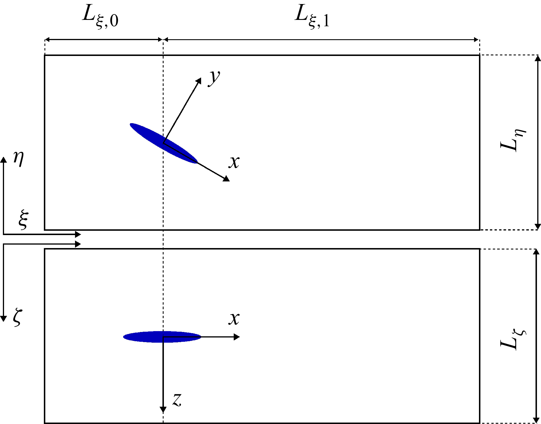


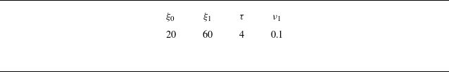


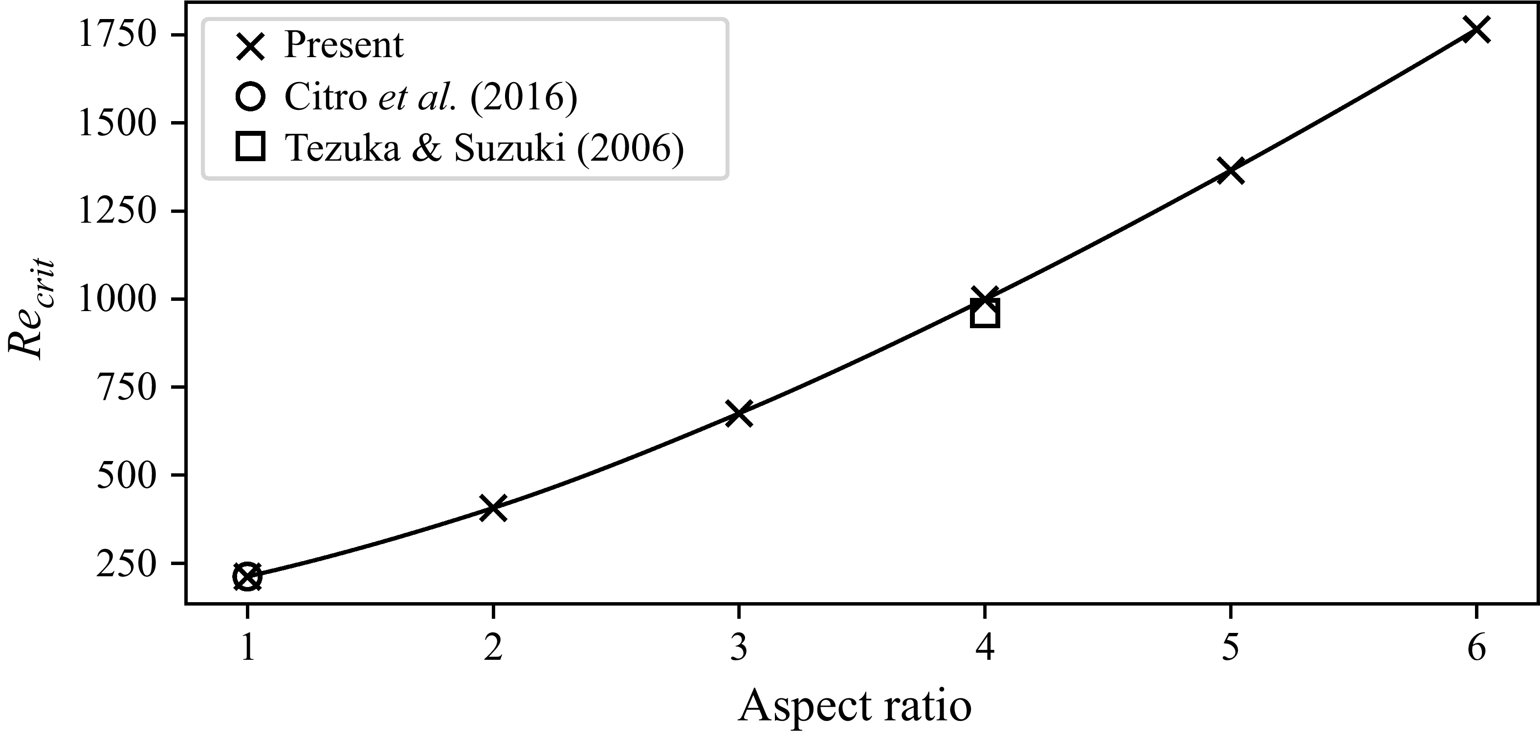


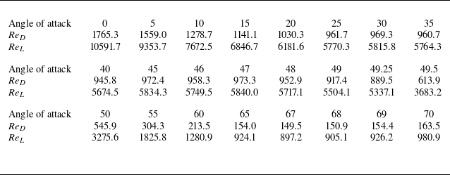
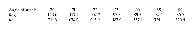


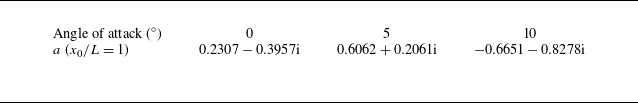


 Open access