4.1. Mean profiles and instantaneous fields

Profiles of mean quantities from cases A–E over the final hour of simulation (between hours 8–9, following Beare et al. Reference Beare2006) are included in figure 2. The mean wind speed profiles $U_h/G = \sqrt {\langle \tilde {u} \rangle ^2 + \langle \tilde {v} \rangle ^2} / \sqrt {U_g^2 + V_g^2}$ (figure 2a) generally increase beyond the background geostrophic wind in the middle of the SBL, with the maximum speed at $z = z_j$ increasing with stability. The mean potential temperature profiles $\varTheta = \langle \tilde {\theta } \rangle$ (figure 2b) display a strong sensitivity to the surface cooling rate, as mean lapse rates increase monotonically from cases A–E for $0.2 \lesssim z/h \lesssim 0.8$. The normalised root-mean-square velocity, $u_{rms} = \sqrt {0.5 (\langle \tilde {u}'^2 \rangle + \langle \tilde {v}'^2 \rangle + \langle \tilde {w}'^2 \rangle )} = e^{1/2}$, where $e$ is the TKE (figure 2c), generally decreases with stability throughout the depth of the SBL likely due in part to the buoyant suppression of TKE with increasing stability.

Figure 2.

Mean profiles from all simulations A–E of (a) horizontal wind speed $U_h = \sqrt {\langle \tilde {u} \rangle ^2 + \langle \tilde {v} \rangle ^2}$ as a fraction of the geostrophic wind vector magnitude $G$ (see table 2), (b) potential temperature $\varTheta = \langle \tilde {\theta } \rangle$ differences from the lowest grid point, (c) root-mean-square resolved velocity $u_{rms} = \sqrt {0.5 (\langle \tilde {u}'^2 \rangle + \langle \tilde {v}'^2 \rangle + \langle \tilde {w}'^2 \rangle )}$, (d) total momentum flux $u_\tau ^2$ (2.1), (e) total potential temperature flux and ( f) gradient Richardson number $Ri_g$, with a reference line at $Ri_g = 0.2$. Statistics are calculated using the final hour of each simulation.

Profiles of the gradient Richardson number (figure 2g),

(4.1)\begin{equation} Ri_g = \frac{g}{\varTheta_0} \frac{\partial \varTheta}{\partial z} \left[ \left(\frac{ \partial \langle \tilde{u} \rangle}{\partial z} \right)^2 + \left(\frac{ \partial \langle \tilde{v} \rangle}{\partial z} \right)^2 \right]^{{-}1}, \end{equation}

in general increase monotonically with surface cooling rate for a given height. The weakly stable cases are largely within the subcritical regime associated with Kolmogorov turbulence, $Ri_g < 0.2$, as identified by Grachev et al. (Reference Grachev, Andreas, Fairall, Guest and Persson2013), whereas simulation E lies above this threshold for $z/h > 0.6$. Finally, the mean profiles of non-dimensional total (resolved plus SGS) momentum and heat flux (figure 2d,e) generally collapse, although the weakly stable cases A and B are more linear than the rest as they are closer to neutral stratification. The irregularities in the lowest grid points for these profiles can be attributed to the wall model. These mean flux profiles are in reasonable agreement with the semi-empirical formulations presented by Nieuwstadt (Reference Nieuwstadt1984) and Sorbjan (Reference Sorbjan1986) that were validated against data from the 1973 Minnesota experiment (Caughey, Wyngaard & Kaimal Reference Caughey, Wyngaard and Kaimal1979).

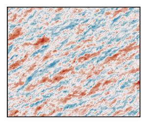
To visually highlight coherent structures within these SBL flows, in figure 3 we present horizontal and vertical cross-sections of the instantaneous fluctuating streamwise velocity and potential temperature fields from simulations A, C and E. Inspection of the horizontal ($x$–$y$) cross-section of $\tilde {u}'/u_{\tau 0}$ located at $z/h=0.05$ (figure 3a–c) indicate elongated streaks of high and low momentum that decrease in size and magnitude with stability. In simulation A (figure 3a) these streaks are $\approx 0.5$–$1.5h$ in length and are rotated with respect to the geostrophic wind (table 2), which is consistent with the streamwise extent of LSMs under neutral and unstable stratification. This is analogous to how HCRs in the CBL are typically rotated $\approx$15–20$^\circ$ to the left of the geostrophic wind due to surface drag and momentum flux divergence (e.g. Salesky et al. (Reference Salesky, Chamecki and Bou-Zeid2017), and references therein). Ansorge & Mellado (Reference Ansorge and Mellado2014) include discussion of these features within stably stratified turbulent flows, but is otherwise beyond the scope of this study. With increasing stability, in cases C and E (figure 3b,c) the velocity field is organised into fine ribbons of weaker fluctuations than in case A, and areas of locally similar magnitudes are less well defined.

Figure 3.

Instantaneous cross-sections from simulations A (left column), C (middle column) and E (right column) including: (a–c) streamwise velocity perturbations and (g–i) potential temperature perturbations in the unrotated $x$–$y$ plane at $z/h=0.05$, and (d–f) streamwise velocity perturbations and (j–l) potential temperature perturbations in the rotated $x'-z$ plane as indicated by the superimposed axes in (a–c) and (g–i). The horizontal lines in (d–f) and (j–l) denote the heights above which $Ri_g \ge 0.2$. The thin angled lines in (d) and (j) annotate the presence of a wall-attached coherent structure.

Unlike streamwise velocity, the horizontal cross-sections of potential temperature fluctuations (figure 3g–i) do not demonstrate corresponding elongated streaks. This result is strikingly different than what is found in the CBL (Salesky et al. Reference Salesky, Chamecki and Bou-Zeid2017), where the vertical velocity and potential temperature fields are visually analogous. Instead, the potential temperature field is composed of a patchy network of warm and cold pockets whose magnitudes depend on stability. In case A there are a few locations where seemingly organised patches of temperature overlap with the long streaks in velocity, e.g. around $(x/h \approx 1, y/h \approx 1)$. It is clear, however, that the frequency of these overlapping patterns is lower in cases C and E than for case A. Here we note that in addition to $\tilde {u}'$ and $\tilde {\theta }'$, cross-sections of $\tilde {w}'$ (not shown) demonstrate generally weak vertical motions without significant organization and, thus, are omitted.

It is apparent from the vertical cross-sections in streamwise coordinates (figure 3d–f) that the elongated velocity streaks extend into the vertical under weak stability. For example, in case A between $0.1 < x'/h < 1.1$, a region of $\tilde {u}'/u_\tau > 0$ extends from the surface up to $z/h \approx 0.25$. These dimensions ($\Delta x'/h \approx 1$, $\Delta z/h \approx 0.25$) correspond to an inclination angle of $\gamma = \arctan (0.25/1) = 14.0^\circ$ with respect to the surface, which agrees well with the values based on two-point correlation statistics as presented by Gibbs et al. (Reference Gibbs, Stoll and Salesky2022) under weakly stable stratification. With increasing stability, however, analogous structures become decreasingly prominent within the flow (figure 3i). The vertical cross-sections of potential temperature fluctuations (figure 3j–l) highlight similar features as those from the streamwise velocity fluctuations. In case A there are elongated regions of high and low perturbations with sharp boundaries in between, which is highly reminiscent of the temperature microfronts presented by Sullivan et al. (Reference Sullivan, Weil, Patton, Jonker and Mironov2016). It is apparent by examining the warm anomaly attached to the surface around $x'/h \approx 0.1$ (corresponding to the one discussed in figure 3d) that the temperature structures do not necessarily incline at the same relative angles as for momentum. As will be discussed further, this eludes to differing mechanisms for vertical transport of heat and momentum under stable stratification. The overall spatial correlation between the momentum and temperature fluctuations in this region align with a sweep of relatively warmer, high-momentum fluid moving towards the surface.

From an analysis of the instantaneous fields presented in figure 3, it is clear that buoyancy acts to suppress vertical organization more strongly than in the horizontal. This has been previously documented (e.g. Huang & Bou-Zeid Reference Huang and Bou-Zeid2013; Chinita, Matheou & Miranda Reference Chinita, Matheou and Miranda2022) and will be important to consider when analysing the results in the following sections.

4.2. Spectrograms

One common method for identifying the presence of coherent structures within turbulent flows is through the analysis of spectrograms (Hutchins & Marusic Reference Hutchins and Marusic2007a; Mathis et al. Reference Mathis, Hutchins and Marusic2009a; Anderson Reference Anderson2016; Baars, Hutchins & Marusic Reference Baars, Hutchins and Marusic2017; Salesky & Anderson Reference Salesky and Anderson2018). Spectrograms are premultiplied power spectra presented as functions of both wavelength and height above the surface, and evidence for LSMs exists when an outer peak is present at large wavelengths. Included in figure 4 are spectrograms for cases A–E of streamwise and vertical velocities, potential temperature and cospectra of $\langle {\tilde {u}'\tilde {w}'} \rangle$ as well as $\langle {\tilde {\theta }'\tilde {w}'} \rangle$.

Figure 4.

Premultiplied spectrograms from simulations A–E (columns) for (a–e) streamwise velocity,( f–j) vertical velocity, (k–o) potential temperature, as well as cospectra of (p–t) $\langle {\tilde {u}'\tilde {w}'} \rangle$ and (u–y) $\langle {\tilde {\theta }'\tilde {w}'} \rangle$. Each is plotted versus streamwise wavelength $\lambda _x$ and wall-normal height $z$ normalised by the SBL depth $h$. Horizontal lines at $\lambda _x = h/4$ indicate the cutoff frequency utilised in the decoupling procedure outlined in § 4.5 that roughly separates the inner and outer peaks (where they exist). Vertical lines are plotted at heights where $Ri_g \ge 0.2$.

Inspection of figure 4 reveals distinct inner and outer peaks in case A across all parameters except for vertical velocity. In case A (figure 4a, f,k,p,u), the outer peak is located approximately at $z/h \approx 0.05$ and $\lambda _x / h \approx 1$, which is as expected within the logarithmic region of the wall-bounded flow at streamwise wavelengths approximately scaling with the flow depth. The wavelength $\lambda _x / h \approx 1$ associated with these outer peaks in case A is also consistent in scale with the velocity streaks in figure 3(a). With this evidence we can reasonably conclude that LSMs are present under weak stability. The outer peak scales are also slightly smaller than those reported by, e.g. Baars et al. (Reference Baars, Hutchins and Marusic2017) for neutrally stratified channel flow, but roughly an order of magnitude smaller than those in the CBL reported by Salesky & Anderson (Reference Salesky and Anderson2018). These differences may likely be due to the lack of VLSMs in the domain considered, so energy peaks at the scale of individual coherent structures instead of a collective superstructure.

For increasing stability, the outer peaks in all of the spectrograms attenuate until they disappear entirely. This behaviour, specifically in streamwise velocity (figure 4a–e), is also in contrast with the findings of Salesky & Anderson (Reference Salesky and Anderson2018), who found that within the CBL, the peak distinctly moved toward smaller wavelengths until it merged with the inner peak with increasing instability. This is undoubtedly the signature of buoyant suppression of vertical motions, which has been shown to act at the large scales (García-Villalba & del Álamo Reference García-Villalba and del Álamo2011) so that large eddies do not traverse the full depth of the SBL. This behaviour is also consistent with the work of Kaimal et al. (Reference Kaimal, Wyngaard, Izumi and Coté1972), who noted decreasing energy at large scales under increasing stability. Recall from the discussion in § 3 and from the results of Li et al. (Reference Li, Salesky and Banerjee2016) that the Ozmidov scale is a characteristic eddy size within the SBL that denotes the beginning of the inertial subrange. Since $L_O$ increases with stability, this implies that the beginning of the inertial subrange shifts towards higher wavenumbers as energy carried by large eddies is damped by buoyancy. This notion is further supported by the lack of an outer peak in the vertical velocity across all cases, although a noticeable ridge does extend from the surface towards larger scales and heights that decreases with increasing stability. The combined effect of these results is evident in the $\langle {\tilde {u}'\tilde {w}'} \rangle$ cospectra (figure 4p–t), indicating a decreasing correlation between $u$ and $w$ with increasing stability. The outer peak in the potential temperature spectrogram $k_x \varPhi _{\theta \theta } / \theta _{\tau 0}^2$ (figure 4k–o) notably is higher in the SBL and occurs at longer wavelengths than those for $u$ for each case. For example, in case B (figure 4l) this peak is centred on $z/h \approx 0.3, \lambda _x/h \approx 1$. Moreover, an outer peak in the potential temperature spectrogram persists through at least case C in similar fashion to the $u$ spectrograms. There also appears to be an outer peak in the $\langle {\tilde {\theta }'\tilde {w}'} \rangle$ cospectra $k_x \varPhi _{\theta w}/\theta _{\tau 0} u_{\tau 0}$ (figure 4u–y) through cases A–C. These differences in momentum and scalar spectrograms indicate underlying differences in their respective transports, which will be discussed further in § 4.4.

Recall from figure 2( f) that the majority of the SBL for cases A–D are in the range $Ri_g < 0.2$, whereas the upper third of the SBL in case E becomes supercritical. Turbulence in these regions is not necessarily persistent in time and is heavily suppressed by buoyancy, thereby inhibiting the development of elongated coherent structures as observed close to the wall. Studies on intermittent turbulence in these regimes typically rely on DNS (e.g. Deusebio et al. Reference Deusebio, Schlatter, Brethouwer and Lindborg2011; Ansorge & Mellado Reference Ansorge and Mellado2014, Reference Ansorge and Mellado2016; Deusebio, Augier & Lindborg Reference Deusebio, Augier and Lindborg2014a; Deusebio et al. Reference Deusebio, Brethouwer, Schlatter and Lindborg2014b; Deusebio, Caulfield & Taylor Reference Deusebio, Caulfield and Taylor2015), as the LES technique can struggle to adequately represent the local nature of turbulence production, transition and dissipation under strong stratification. Herein we therefore take extra caution when interpreting further results from these regions of supercritical stability.

From these spectrograms, it is apparent that buoyancy acts strongly to attenuate vertical motions at large streamwise wavelengths, resulting in turbulence that is increasingly local with increasing stability. There is evidence that velocity and potential temperature organise into large-scale coherent structures through at least case C (recall from table 1 that $C_r = 0.33$ K h$^{-1}$, $h/L=1.83$) based on the presence of outer peaks. In § 4.3 we explore further how these fields are affected by stability across scales.

4.3. Linear coherence spectra

In addition to spectrograms, another method of diagnosing the relevant scales affected by coherent structures is through computation of the linear coherence spectrum (LCS; Baars et al. Reference Baars, Hutchins and Marusic2017). The LCS is a measure of the linear coupling between variables across scales, and is defined as

(4.2)\begin{equation} \gamma_{uu}^2(z,z_R;\lambda_x) = \frac{| \langle \hat{u}(z;\lambda_x) \hat{u}^*(z_R;\lambda_x) \rangle_{yt} |^2}{\langle |\hat{u}(z;\lambda_x)|^2 \rangle_{yt} \langle |\hat{u}(z_R;\lambda_x)|^2 \rangle_{yt}}, \end{equation}

where $\hat {u}(z;\lambda _x) = \mathcal {F} \{ u(x,z) \}$ is the Fourier transform of $u(x,z)$ along the streamwise dimension with the asterisk $*$ denoting its complex conjugate, $z_R$ represents a constant reference height above ground level for comparison against all heights $z$ and $|{\cdot }|$ refers to the modulus of a complex value. In this context, $\gamma _{uu}^2$ falls within the range $\gamma _{uu}^2 \in [0, 1]$, and can be interpreted as the squared value of the correlation coefficient at a specific scale $\lambda _x$ between fluctuating values of $u$ at two different heights $z$ and $z_R$. An example of this is included in figure 5, where we calculate $\gamma _{uu}^2$ and $\gamma _{\theta \theta }^2$ using a reference height $z_R = \varDelta _z/2$ as the lowest grid point in each simulation. The strongest coupling across all simulations and parameters is noticeably found at horizontal wavelengths of $O(h)$, as was found with the outer peaks in the premultiplied spectrograms in the previous section. Moreover, the vertical extent of the LCS peaks diminishes with increasing stability. For example, $\gamma _{uu}^2$ for case A extends beyond $z/h=0.1$ whereas by case C the contour for $\gamma _{uu}^2=0.1$ only extends to $z/h \approx 0.04$. The $\gamma _{uu}^2$ and $\gamma _{\theta \theta }^2$ peaks for case A (figure 5a, f) can also be attributed to the coherent features identified in the instantaneous fields that extend from the surface up into the outer region of the flow (figure 3a,e). We note here that due to vertical resolution limitations using a wall-modelled LES, the contours near the surface do not provide significant amounts of information at higher stabilities. Baars et al. (Reference Baars, Hutchins and Marusic2017) argue that a 1 : 1 slope of these peaks in log-log coordinates, specifically in streamwise velocity under near-neutral stratification (case A), is consistent with the attached-eddy hypothesis (Townsend Reference Townsend1976) across a self-similar hierarchy of scales. Analysis of these cases in the framework of the attached-eddy hypothesis is beyond the scope of this study, but certainly warrants further investigation, ideally with higher resolutions close to the wall.

Figure 5.

Linear coherence spectra for (a–e) $u$, ( f–j) $w$ and (k–o) $\theta$ for cases A–E (columns) calculated with the reference point $z_R$ as the lowest grid point and plotted against non-dimensional wavelength and wall-normal distance. The horizontal line in each panel is the same as in figure 4.

It is also possible to define (4.2) for two independent variables at the same height, which provides information on the coupling of two parameters across scales. For example, the LCS between $u$ and $w$ at wall-normal distance $z$ would be determined as $\gamma _{uw}^2 = \gamma _{uw}^2(z,z;\lambda _x)$. The resulting values of $\gamma _{uw}^2$ and $\gamma _{\theta w}^2$ are included in figure 6 for cross-sections at constant heights $z/h$ within the SBL. Near the top of the surface layer ($z/h=0.1$, figure 6a) it is apparent that the coupling between $u$ and $w$ is strongest for $\lambda _x / h \ge 0.5$ in all cases. With increasing stability, the maximum in $\gamma _{uw}^2$ monotonically shifts towards smaller wavelengths and decreases in magnitude from a value of $\approx 0.4$ in case A to $\approx 0.3$ in case E. The magnitude of $\gamma _{uw}^2$ for wavelengths larger than their respective peaks also decreases monotonically with increasing stability. For vertical transport of potential temperature at this height (figure 6c), the impacts from buoyancy are noticeable in the attenuation of $\gamma _{\theta w}^2$ with increasing stability at larger scales ($\lambda _x/h > 0.5$). In general, we observe that the peaks at this height for $\gamma _{uw}^2$ are larger than those for $\gamma _{\theta w}^2$, but at small wavelengths $\lambda _x/h < 0.1$ this trend is reversed.

Figure 6.

Cross-sections of LCS from cases A–H at constant heights: (a,c) $z/h=0.1$ and (b,d) $z/h=0.25$ for (a,b) $\gamma _{uw}^2$ and (c,d) $\gamma _{\theta w}^2$. Vertical lines at $\lambda _x / h = 0.25$ are included for reference.

Higher in the SBL at $z/h = 0.25$ (figure 6b,d), we largely observe the same patterns in $\gamma _{uw}^2$ and $\gamma _{\theta w}^2$ as those for $z/h = 0.1$ but with slightly smaller peak values at high stability. These results again reflect how buoyancy suppresses vertical transport of both momentum and heat at large scales, but the differences in $\gamma _{uw}^2$ and $\gamma _{\theta w}^2$ at fine scales allude to differing transport mechanisms. This topic is discussed in further detail in § 4.4.

4.4. Transport efficiency

In § 4.2 we identified the existence of an outer peak in the premultiplied spectrograms in cases A–C, and in § 4.3 found enhanced linear coupling at the scales of these outer peaks. Previous studies of the CBL have shown that turbulent transports of momentum and scalars become increasingly dissimilar with increasing instability (Li & Bou-Zeid Reference Li and Bou-Zeid2011; Dupont & Patton Reference Dupont and Patton2012; Patton et al. Reference Patton, Sullivan, Shaw, Finnigan and Weil2016; Salesky Reference Salesky2023), and Salesky et al. (Reference Salesky, Chamecki and Bou-Zeid2017) were able to connect this breakdown of Reynolds’ analogy to varying modes of convective organization. However, the relationship between momentum and heat transport in stably stratified turbulent shear flows remains relatively unexplored. To study these effects, it is useful to consider the partitioning of turbulent fluxes into contributions by individual positive and negative fluctuations in either term. This technique is known as quadrant analysis (also conditional sampling; see Wallace (Reference Wallace2016), and references therein), and is outlined as follows. Using the resolved vertical momentum flux $\langle {\tilde {u}'\tilde {w}'} \rangle$ as an example, we define the four quadrants as

• (i) Quadrant I: $\tilde {u}' > 0, \tilde {w}' > 0$,

• (ii) Quadrant II: $\tilde {u}' < 0, \tilde {w}' > 0$,

• (iii) Quadrant III: $\tilde {u}' < 0, \tilde {w}' < 0$,

• (iv) Quadrant IV: $\tilde {u}' > 0, \tilde {w}' < 0$.

With this definition, quadrants II and IV are respectively referred to as ejections and sweeps. The quadrants for potential temperature flux are defined likewise by replacing $u$ with $\theta$, and for stable thermal stratification, quadrants II and IV also refer to the downgradient direction. The turbulent transport efficiencies based on these quadrants are defined based on the fraction of the total flux occurring in the downgradient direction (Wyngaard & Moeng Reference Wyngaard and Moeng1992; Li & Bou-Zeid Reference Li and Bou-Zeid2011; Salesky et al. Reference Salesky, Chamecki and Bou-Zeid2017). For the SBL where $\partial U_h / \partial z > 0$ and $\partial \varTheta / \partial z > 0$, the transport efficiencies for momentum and heat are defined (adopting the notation of the present paper) as

(4.3)\begin{equation} \eta_{uw} = \frac{\langle {\tilde{u}'\tilde{w}'} \rangle}{\langle {\tilde{u}'\tilde{w}'} \rangle^{II} + \langle {\tilde{u}'\tilde{w}'} \rangle^{IV}} \end{equation}

and

(4.4)\begin{equation} \eta_{\theta w} = \frac{\langle {\tilde{\theta}'\tilde{w}'} \rangle}{\langle {\tilde{\theta}'\tilde{w}'} \rangle^{II} + \langle {\tilde{\theta}'\tilde{w}'} \rangle^{IV}}. \end{equation}

Here the superscripts II and IV refer to the individual quadrant contributions to the total flux from specifically quadrants II and IV. Note that we intentionally neglect the SGS flux contributions in (4.3) and (4.4) for use with LES output, as the quadrant assignment for, e.g. $\tau _{xz}$ is not directly discernible from the signs of $\tilde {u}'$ and $\tilde {w}'$.

Profiles of these transport efficiencies along with their ratio are displayed in figure 7. There is a modest dependence on stability for both $\eta _{uw}$ and $\eta _{\theta w}$ that is most apparent in the profile of their ratio (figure 7c). The ratio $\eta _{uw}/\eta _{\theta w}$ is close to unity for $0.2 < z/h < 0.6$ for all cases A–E, and generally does not vary with stability in the layer $z/h < 0.2$. For $z/h > 0.6$, this ratio has a strong dependence on stability as $\eta _{\theta w}$ does not decrease as sharply with height for cases C–E as compared with cases A and B. In general, this decrease with height in $\eta _{uw}$ is mostly consistent across cases for this region of the SBL. In the middle of the SBL, there is a minor dependence on both $\eta _{uw}$ and $\eta _{\theta w}$ with stability, for example, at $z/h=0.4$ both transport efficiencies are highest for case A and lowest for case E. Closer to the surface ($z/h=0.05$), this trend is somewhat reversed. Regardless of these differences, the transport efficiencies in both momentum and heat are markedly lower than those reported in both observed and simulated CBLs at weak instability (e.g.  Li & Bou-Zeid Reference Li and Bou-Zeid2011; Salesky et al. Reference Salesky, Chamecki and Bou-Zeid2017). Therefore, it is apparent that even weak stratification plays a strong role in inhibiting the flow's ability to vertically redistribute momentum or heat.

Figure 7.

Profiles of transport efficiencies (a) $\eta _{uw}$ (4.3), (b) $\eta _{\theta w}$ (4.4) and (c) their ratio $\eta _{uw}/\eta _{\theta w}$ for cases A–E.

These differences in transport efficiencies can be traced to changes in turbulent motions from each quadrant I–IV as displayed in figure 8. Plotted here are the individual quadrant fractions $Q_{uw}^k$ and $Q_{\theta w}^k$, which are defined as

(4.5)\begin{equation} Q_{uw}^k = \frac{| \langle {\tilde{u}'\tilde{w}'} \rangle^k |}{\sum | \langle {\tilde{u}'\tilde{w}'} \rangle^k |} \end{equation}

and

(4.6)\begin{equation} Q_{\theta w}^k = \frac{| \langle {\tilde{\theta}'\tilde{w}'} \rangle^k |}{\sum | \langle {\tilde{\theta}'\tilde{w}'} \rangle^k |}, \end{equation}

where $k \in \{ \mathrm {I, II, III, IV}\}$ represents the individual quadrant contributions to the absolute sum.

Figure 8.

Individual quadrant fractions (a–d) $Q_{uw}^k$ (4.5) and (e–h) $Q_{\theta w}^k$ (4.6) for cases A–E. Vertical lines at $Q^k=0.25$ are included for reference.

Recalling that quadrants II and IV in the momentum flux (figure 8b,d) denote ejections and sweeps, respectively, it is apparent that motions in these quadrants dominate the total flux profile with quadrant fractions $Q_{uw}^{II}, Q_{uw}^{IV} > 0.25$ for all cases A–E. The fraction of ejections remains roughly constant with height for each case for $0.1 < z/h < 0.8$, whereas the sweeps decrease with height in this range. In the range $0.1 < z/h < 0.9$, the fraction of ejections also tends to decrease gradually with stability, and the upper bound on this range also decreases with stability as the profiles break towards $Q_{uw}^{II}=0.25$ at progressively lower heights. In the upper half of the SBL, the decreasing ejections with stability are primarily compensated for in the countergradient motions of quadrant I and by sweeps (figure 8a,d). The differences in quadrant III (figure 8c) are comparatively smaller with changes in stability, indicating that changes in transport efficiency largely depend on how positive vertical motions interact with relatively high or low streamwise momentum parcels within the SBL. At the top of the SBL ($z/h \approx 1$), all four quadrants reach equilibrium with an even distribution of $Q_{uw}^k = 0.25$.

The heat flux profiles display a somewhat different pattern, however, with quadrants II and IV dominating the contributions at all levels (figure 8f,h). Otherwise, the general trends in the heat flux quadrant fractions are largely similar to those of momentum fluxes: ejections (upwelling relatively cold parcels) are relatively constant with height whereas sweeps decrease with height, reaching a minimum around $z/h \approx 0.85$. In the middle of the SBL around $z/h \approx 0.5$, the thermal ejections decrease in fraction with stability, which is accounted for by an increase in countergradient motions in quadrants I and IV at this level whereas quadrant III is relatively invariant (similar to those for momentum).

We explore the contributions to each quadrant further by examining joint probability density functions (JPDFs) and their corresponding covariance integrands. These two are related by considering two random variables $a$ and $b$ such that their covariance $\langle a'b' \rangle = \int _{-\infty }^{\infty } abP(a,b) \,\mathrm {d}a \,\mathrm {d}b$ depends on their JPDF, $P(a,b)$ (Wallace Reference Wallace2016). By considering both of these quantities we can identify the pairs of, e.g. $u'$ and $w'$ that contribute most strongly to each quadrant fraction $Q_{uw}^k$.

The JPDFs and their covariance integrands of $uw$ and $\theta w$ are included in figure 9 for cases A, C and E at heights of $z/h = 0.1$ and $0.5$. Corresponding to the decrease in $uw$ ejections (figure 8b), it is apparent from figure 9(a,e,i) that the quadrant II peak in $uwP(u,w)$ shifts towards smaller values of $u'/u_{\tau 0}$ and $w'/u_{\tau 0}$ with increasing stability. Additionally, the extent of $uwP(u,w)$ in quadrant IV reaches towards larger values of $u'/u_{\tau 0}$ with increasing stability, which accounts for the increase in $Q_{uw}^{IV}$ at $z/h=0.1$. These changes are even more drastic at $z/h=0.5$ (figure 9b, f,j), where the quadrant I peak of $uwP(u,w)$ increases in magnitude with stability as the quadrant II peak weakens and the overall distribution of $u'$ and $w'$ becomes more evenly distributed in all four quadrants.

Figure 9.

Joint PDFs and their premultiplied covariance integrands selected at (first and third columns) ${z/h=0.1}$ and (second and fourth columns) $z/h=0.5$ for cases (row one) A, (row two) C and (row three) E. Joint PDFS are shaded in greyscale, and the covariance integrands are overlaid in red and blue contours. Included are (first two columns) $uw$ and (last two columns) $\theta w$.

The joint distribution of $\theta$ and $w$ at $z/h=0.1$ does not change drastically with stability (figure 9c,g,k), which is expected given their quadrant fractions observed in figure 8. In the middle of the SBL, however, these distributions are extremely sensitive to increasing stability (figure 9d,h,l). The spread in values of $w'/u_{\tau 0}$ decreases markedly with stability, most notably in quadrants II and IV in $\theta wPDF(\theta,w)$, and there is not a corresponding decrease in the spread of $\theta '/\theta _{\tau 0}$. Additionally, the peaks of $\theta wPDF(\theta,w)$ tend towards smaller values of $|\theta '/\theta _{\tau 0}|$ and $|w'/u_{\tau 0}|$ in all quadrants, which corresponds to overall weaker and less efficient transport of heat in the middle of the SBL (figure 7b).

It is apparent from the turbulent transfer efficiencies (figure 7), individual quadrant fractions (figure 8) and JPDFs (figure 9) that momentum and heat are transported differently as stability increases. Under weakly stable stratification (case A), our results generally match those from Li & Bou-Zeid (Reference Li and Bou-Zeid2011) and Salesky et al. (Reference Salesky, Chamecki and Bou-Zeid2017) under weakly unstable conditions. Therefore, it is likely that coherent turbulent structures such as hairpin vortices exist in case A (Adrian Reference Adrian2007), but increasing stratification flattens motions into largely horizontal features. Vertical motions become more localised and contributions from countergradient fluxes reduce the overall efficiencies in turbulent transport of both momentum and heat. This is also consistent with the small-scale circulations around microfronts in the SBL as observed by Sullivan et al. (Reference Sullivan, Weil, Patton, Jonker and Mironov2016) from their high-resolution LES.

4.5. Amplitude modulation

To further examine how LSMs affect the smaller scales within the SBL, in this section we perform the decoupling procedure outlined by Mathis et al. (Reference Mathis, Hutchins and Marusic2009a) and more recently by Salesky & Anderson (Reference Salesky and Anderson2018). The decoupling procedure as implemented with single-point correlations is summarised as follows.

First we consider two random variables $a=a(z;t)$ and $b=b(z;t)$. We are interested in computing the extent to which the large scales of signal $b$ at height $z$ modulate the small-scale amplitude of signal $a$ also at height $z$. To extract the large-scale components of these signals $a_l$ and $b_l$, we lowpass filter each such that $a_l(z;t) = G * a(z;t)$, where $G$ is the impulse response function of a sharp spectral filter that is convolved with $a$. For the present study, we define the filter function to have a cutoff wavelength equal to half the height of the LLJ, $\lambda _c = h/4$, which generally is in the range separating the inner and outer peaks in the premultiplied spectrograms (figure 4). We further extract the small-scale component of each signal as $a_s(z;t) = a(z;t) - a_l(z;t)$.

The next step involves a Hilbert transform $\mathcal {H}$, which for the small-scale signal $a_s$, is defined as

(4.7)\begin{equation} \mathcal{A}_s(t) = \mathcal{H}\{ a_s(t)\} = \frac{1}{\rm \pi}\mathcal{P} \int_{-\infty}^{+\infty} \frac{a_s(\tau)}{t - \tau}\, {\rm d}\tau, \end{equation}

where $\mathcal {P}$ is the Cauchy principal value of the integral for time shift $\tau$. Mathematically, (4.7) is the convolution integral between $a_s(t)$ and the quantity $1/{\rm \pi} t$ such that $\mathcal {A}_s(t) = a_s(t) * (1/{\rm \pi} t)$. From the fundamental properties of the Hilbert transform (Mathis et al. Reference Mathis, Hutchins and Marusic2009a; Bendat & Piersol Reference Bendat and Piersol2010), $a_s(t)$ and $\mathcal {A}_s(t)$ form a complex analytic signal $Z(t)$ such that

(4.8)\begin{equation} Z(t) = a_s(t) + i\,\mathcal{A}_s(t) = A_s(t)\,\mathrm{e}^{{\rm i}\phi_s(t)}, \end{equation}

where $A_s(t)$ and $\phi _s(t)$ are the instantaneous modulus and phase of $Z(t)$ (Sreenivasan Reference Sreenivasan1985; Tardu Reference Tardu2008; Mathis et al. Reference Mathis, Hutchins and Marusic2009a). The modulus $A_s (t)$ of the analytic signal,

(4.9)\begin{equation} A_s(t) = \sqrt{a_s^2(t) + \mathcal{A}_s^2(t)}, \end{equation}

represents the envelope of the original signal, $E(a_s)$. Next, we lowpass filter the envelope of $a_s$ such that $E_l(a_s) = G * E(a_s)$, which is the final element required to determine the AM coefficients.

The AM coefficient in this example is given as the correlation coefficient between the large-scale component of $b$ and the large-scale component of the envelope of small-scale $a$, i.e.

(4.10)\begin{equation} R_{b_l,a_s}(z) = \frac{\langle b_l'(z;t) E_l'(a_s(z;t)) \rangle_{t}}{\sqrt{\langle b_l'^2(z;t) \rangle_{t}} \sqrt{\langle E_l'^2(a_s(z;t)) \rangle_{t}}}. \end{equation}

We note that (4.10) differs from that presented by Salesky & Anderson (Reference Salesky and Anderson2018) in generality since they considered both two- and one-point statistics, whereas in this present study we consider only one-point AM coefficients (i.e. at the same height). Their results indicate that the one-point statistics provide a stronger signal in terms of correlations when compared with the two-point AM coefficients. Since increasing stability further limits vertical turbulent transport, we expect two-point AM coefficients in the present study to be small.

For the decoupling procedure to be implemented appropriately, there needs to be adequate scale separation between the inner and outer peaks (Mathis et al. Reference Mathis, Hutchins and Marusic2009a). Investigation of figure 4 indicates this condition is only met for cases A–C, with cases D and E ($C_r = 0.50,\ 1.00$ K h$^{-1}$, $h/L = 2.49, 4.17$, respectively) on the fringe. Herein, we present results using virtual tower output at 50 Hz frequency from cases A–E with the added caveat of marginal scale separation existing in cases D and E. In figure 10 we include the AM coefficients between large-scale $u_l$ and $w_l$ with small-scale $u_s$, $w_s$, $\theta _s$, $(uw)_s$ and $(\theta w)_s$. The AM coefficients are presented for each case as functions of wall-normal distance $z/h$ to identify the role of global stability on coupling between the large and small scales. As one can discern from the AM by large-scale $u_l$ (figure 10a–e), the largest correlations are found in the upper portion of the SBL, namely for $z/h > 0.4$. In this region, the values of $R$ are mostly negative and decrease moderately in magnitude with stability for a given height. Using the example of $R_{u_l,u_s}$ (figure 10a), a positive correlation near the surface can physically be interpreted as follows: the small-scale velocity $u_s$ increases due to modulation by a high-momentum LSM with $u_l > 0$, or decreases due to modulation by a low-momentum LSM with $u_l < 0$. Conversely, a negative correlation implies that on average, a high-momentum LSM will act to suppress small-scale perturbations, and a low-momentum LSM will excite small-scale perturbations. For the weakly stable case A, $R_{u_l,u_s}$ is negligible near the surface, decreases towards small negative values around $z/h \approx 0.2$ and further decreases to $R_{u_l,u_s} \approx -0.2$ in the upper half of the SBL. This behaviour is consistent with both the weakly convective case presented by Salesky & Anderson (Reference Salesky and Anderson2018) as well as the neutrally stratified case by Mathis et al. (Reference Mathis, Monty, Hutchins and Marusic2009b). This similarity also holds for all the other AM coefficients with modulation by $u_l$ except for $R_{u_l,\theta _s}$ (figure 10c), which is weakly positive throughout most of the SBL across all cases. In terms of overall magnitude for modulations by $u_l$, the largest impact is observed near the top of the SBL for $R_{u_l,(uw)_s}$, which reaches values as low as $-0.4$ in cases A and B (figure 10d). Negative coupling between large- and small-scale streamwise velocity at these heights is most likely associated with turbulence production by the LLJ.

Figure 10.

The AM coefficients $R$ from cases A–E bin averaged versus $z/h$ for correlations with (a–e) $u_l$ and ( f–j) $w_l$. Small-scale envelopes include (a, f) $u_s$, (b,g) $w_s$, (c,h) $\theta _s$, (d,i) $(uw)_s$ and (e,j) $(\theta w)_s$.

By contrast, the AM coefficients for large-scale vertical velocity $w_l$ (figure 10f–j) are markedly smaller than those for $u_l$ across all cases. The only non-negligible coefficients occur under weak stability (cases A and B) for coupling between $w_l$ and the instantaneous second-order moments $(uw)_s$ and $(\theta w)_s$ (figure 10i,j) for the near-neutral case A. Even these values are modest, however, and again may likely be associated with turbulent transport below the LLJ. These weak $w_l$ AM coefficients may also stem from to the lack of an appreciable outer peak in the vertical velocity spectrograms of cases D and E (figure 4f–j).

There are a few core similarities and differences between the AM coefficients displayed in figure 10 versus those presented by Salesky & Anderson (Reference Salesky and Anderson2018) under varying convective stratifications. First, the coupling with small-scale instantaneous momentum flux $(uw)_s$ is the largest observed among all considered combinations of parameters in both the CBL and SBL. Moreover, the correlations with large-scale $w_l$ were relatively unaffected by global stability in both the CBL and SBL. However, in the SBL this is because the correlations were negligible across all simulations, whereas they were substantial in the CBL. With increasing stability, the results from figure 10 indicate that AM may occur due to large-scale $u_l$ but not necessarily for $w_l$, which is also consistent with the notion that buoyancy suppresses large-scale vertical motions (e.g. García-Villalba & del Álamo Reference García-Villalba and del Álamo2011).

In an attempt to better characterise the effects of local stability on AM, included in figure 11 are the AM coefficients plotted against $Ri_g$. Recall from figure 2( f) that $Ri_g$ nearly monotonically increases with height and stability for cases A–E throughout the SBL. We composited all five simulations A–E and bin averaged the AM coefficients based on evenly logarithmically spaced bins in $Ri_g$ with vertical error bars denoting the standard deviation of each bin in figure 11. It is apparent that on average, $u_l$ weakly correlates positively with small-scale parameters under weak local stability ($Ri_g < 0.05$, figure 11a–e), and these correlations decrease and eventually become negative under higher stability ($Ri_g > 0.1$). The largest spread in the correlations with $u_l$ occur around the critical Richardson number (Grachev et al. Reference Grachev, Andreas, Fairall, Guest and Persson2013), $Ri_g \approx 0.2$. All of these AM coefficients tend to level off with further increasing stability at relatively small values $-0.1 < R < 0.1$. The correlations with large-scale $w_l$ (figure 11f–j) are virtually zero for $Ri_g > 0.01$ across all parameters.

Figure 11.

As in figure 10 but composited across all cases and plotted against $Ri_g$. Bin medians are plotted in blue and means in black with error bars denoting $\pm 1$ standard deviation.

The results following from the decoupling procedure discussed in this section are consistent with those throughout this study and in the literature: negative buoyancy in the SBL suppresses vertical motions at large scales, forcing coherent structures to become increasingly confined to horizontal planes and at increasingly local scales (recall figure 1a).

4.6. Conditional averaging

A common feature of LSMs in wall-bounded flows is their association with low- and high-speed streaks in the logarithmic layer (Adrian Reference Adrian2007), so it is therefore advantageous to composite snapshots of the flow when these conditions are present. This process is known as conditional sampling (Antonia Reference Antonia1981), which we can define for the streamwise velocity (in notation following Salesky & Anderson (Reference Salesky and Anderson2020), and with adapted conventions) as

(4.11)\begin{equation} \frac{\tilde{u}'^{{\dagger}}(\boldsymbol{x},t)}{u_{\tau 0}} = \left\langle \left.\frac{\tilde{u}'(\boldsymbol{x},t)}{u_{\tau 0}} \right| \frac{\tilde{u}'(\boldsymbol{x}_c,t)}{u_{\tau 0}} <{-}2 \frac{\sigma_{\tilde{u}'(\boldsymbol{x}_c)}}{u_{\tau 0}} \right\rangle_{N_{\alpha^-}}, \end{equation}

where $\tilde {u}'^{{\dagger}} (\boldsymbol {x},t)/u_{\tau 0}$ is the streamwise velocity averaged over $N_{\alpha ^-}$ instances where the flow is below the threshold $\alpha ^- = -2 \sigma _{\tilde {u}'(\boldsymbol {x}_c)}/u_{\tau 0}$ at the coordinate $\boldsymbol {x}_c = (x', y', z=0.05h)$ and $\sigma _{\tilde {u}'(\boldsymbol {x}_c)}$ is the standard deviation of velocity fluctuations. Here, $({\cdot })^{{\dagger}}$ is used to denote a conditionally averaged variable.

Conditionally averaged streamwise velocity, vertical velocity and potential temperature fields based on $\alpha ^-$ in (4.11) are included in figure 12 for cases A–E. The effects of stability are immediately apparent in all three averaged fields, with the extent of the conditionally averaged coherent structures diminishing in spatial extent (both horizontally and vertically) with increasing stability. In case A the streamwise extent of the central $\tilde {u}'^{{\dagger}} /u_{\tau 0}$ feature is $\approx 2h$, which corresponds well to the wavelength associated with the outer peak in the streamwise velocity spectrogram (figure 4a) of $\lambda _x / h \approx 1$–2. When conditioning on low-speed streaks near the surface, the $\tilde {u}'^{{\dagger}} /u_{\tau 0}$ minimum extends vertically up to $z/h \approx 0.3$ in case A, and appears to tilt upwards downstream from the central peak (figure 12a). This $\tilde {u}'^{{\dagger}} /u_{\tau 0}$ minimum diminishes under increasing stratification until the conditional low-speed streak becomes confined vertically and longitudinally (follow figure 12a,d,g,j,m sequentially). Combined with the evidence from the spectrograms, these results largely agree with the conceptual model of LSMs by, e.g. Marusic et al. (Reference Marusic, Mathis and Hutchins2010a). Interestingly, the corresponding field of $\tilde {w}'^{{\dagger}} /u_{\tau 0}$ in case A (figure 12b) features a maximum in vertical velocity directly overlaid with the low-speed streak, which highlights the dynamics of an ejection (recall § 4.4) in both momentum and temperature (figure 12c). These $\tilde {w}'^{{\dagger}} /u_{\tau 0}$ features include a similar downstream inclination as those in the $\tilde {u}'^{{\dagger}} /u_{\tau 0}$ minima, but also exhibit another vertically extending lobe upstream. The vertical and horizontal extents of these upstream and downstream lobes, respectively, decrease rapidly with increasing stratification. The correlation between $u$ and $\theta$ throughout the SBL is highlighted by how similarly the $\tilde {u}'^{{\dagger}} /u_{\tau 0}$ and $\tilde {\theta }'^{{\dagger}} /\theta _{\tau 0}$ fields evolve under increasing stability, as they are nearly identical qualitatively. In combination with the asymmetrical distribution of $\tilde {w}'^{{\dagger}} /u_{\tau 0}$, this again may be related to the presence of temperature microfronts (Sullivan et al. Reference Sullivan, Weil, Patton, Jonker and Mironov2016) within the SBL that concentrate gradients in velocity and temperature.

Figure 12.

Average fields conditioned on $\tilde {u}'/u_{\tau 0} < \alpha ^-$ as in (4.11) from simulations (a–c) A, (d–f) B, (g–i) C, (j–l) D and (m–o) E. Conditional fields include (a,d,g,j,m) $\tilde {u}'^{{\dagger}} /u_{\tau 0}$, (b,e,h,k,n) $\tilde {w}'^{{\dagger}} /u_{\tau 0}$ and (c, f,i,l,o) $\tilde {\theta }'^{{\dagger}} /\theta _{\tau 0}$. Here $\Delta x'$ represents the distance upstream and downstream from each instance meeting the conditioning criteria of a low-speed streak.

The conditionally averaged fields in figure 12 are a visual representation of the statistical results presented in §§ 4.2–4.5: buoyancy suppresses large-scale vertical circulations within SBL flows. Even under weak stability, the updrafts associated with ejections do not penetrate far above the surface and are roughly 70 % as wide as their corresponding low-speed streaks and cold air parcels. These fields are also reminiscent of the two-point correlations of $u$ and $w$ presented by Huang & Bou-Zeid (Reference Huang and Bou-Zeid2013), which identified elongated coherence in the streamwise direction in the lower SBL. A similar analysis of our simulations (not shown) demonstrated the same pattern, which also decreased in extent with increasing stability.