


1. Introduction
The impact of a drop on a liquid pool has served as one of the canonical problems of free surface flows for over a century since the pioneering work of Worthington (Reference Worthington1882), which explored the dynamics of an impacting drop and the subsequent jet using high-speed photography. The studies on the classical impacts of a single liquid drop (Engel Reference Engel1966; Prosperetti & O $\tilde{g}$uz Reference Prosperetti and Og̃uz1993; Leng Reference Leng2001) and a solid object (Gilbarg & Anderson Reference Gilbarg and Anderson1948; Aristoff & Bush Reference Aristoff and Bush2009; Truscott, Epps & Belden Reference Truscott, Epps and Belden2014) onto a liquid pool have revealed a variety of fascinating dynamic processes of liquid splashes and air cavities. In addition, prior investigations on the impacts of fragmented shaped charges onto a solid target (Birkhoff et al. Reference Birkhoff, MacDougall, Pugh and Taylor1948) and multiple drops on a liquid pool (Bick et al. Reference Bick, Ristenpart, van Nierop and Stone2010) have shown how the interaction of multiple incoming bodies affect the dynamic responses of the target surfaces. Here, we study the dynamic response of a water surface to the impact of a drop train, i.e. a series of identical liquid drops with a constant frequency. The impact of a drop train not only generates interfacial phenomena distinct from those by a single drop impact, but is also practically relevant to a semiconductor cleaning process. The successive collision of microdrops with a liquid film covering a semiconductor wafer continually generates pressure waves, which are supposed to remove the contaminant particles from the solid surface (Kondo & Ando Reference Kondo and Ando2019).
When drops impact successively on a liquid pool with a sufficiently high frequency, a slender cavity is generated (Hurd et al. Reference Hurd, Fanning, Pan, Mabey, Bodily, Hacking, Speirs and Truscott2015). Six different types of cavities were identified by Speirs et al. (Reference Speirs, Pan, Belden and Truscott2018) depending on the drop impact frequency, the maximum expansion time of a crater owing to a single drop impact and the Weber number. Bouwhuis et al. (Reference Bouwhuis, Huang, Chan, Frommhold, Ohl, Lohse, Snoeijer and van der Meer2016) numerically computed the shape and growth rate of the slender cavity produced by micrometre-sized drops and compared the results with experiment. The elongation rate of the cavity was found to be constant during its growth and to depend on the impact velocity of drops and a dimensionless frequency,  $\phi =fd/U$, which corresponds to a ratio of the drop diameter ( $d$) to the centre-to-centre spacing of adjacent drops ( $U/f$). Here, $U$ and $f$ are the impact velocity and generation frequency of drops, respectively.
The elongation of the cavity ceases when it closes, owing to pinch-off near the free surface. The pinch-off occurs when capillary forces near the cavity neck prevail over inertia of the growing cavity. Speirs et al. (Reference Speirs, Pan, Belden and Truscott2018) obtained the maximum depth of the cavity before the pinch-off by balancing the surface potential energy with the kinetic energy. However, no account has been given yet to the shape of the liquid surface after pinch-off under a continual impact of the drop train.
The goal of our study is to provide physical insights and experimental results to further our understanding of the dynamics of a liquid surface under the impact of a drop train. First, we aim to construct an analytical model to predict the growth rate and the profile of the cavity arising from the impact of a drop train when inertia dominates over viscosity, gravity and capillarity. The model will explain the dynamics of cavity growth by going beyond the prior numerical (Bouwhuis et al. Reference Bouwhuis, Huang, Chan, Frommhold, Ohl, Lohse, Snoeijer and van der Meer2016) and simple (Speirs et al. Reference Speirs, Pan, Belden and Truscott2018) models. Second, we describe the shape of the liquid surface after a collapse of the cavity and mathematically elaborate the interfacial topography. This corresponds to the steady-state response of the liquid surface to the impact of the drop train.
2. Experimental
Figure 1 shows the experimental set-up to generate a stream of uniform drops and to investigate the deformation of a liquid surface upon impact of the drops. The liquid tank was pressurised by nitrogen to produce a jet of liquid from a nozzle, which was vibrated using a piezoelectric transducer driven by an amplifier connected to a function generator (Kim, Park & Min Reference Kim, Park and Min2003). The jet was broken up into uniform drops at a frequency set by the function generator (AFG3021B, Tektronix). The drop train then impacted on a pool of the identical liquid. The dynamic interaction of the drops and the liquid pool was recorded by a high-speed camera (Fastcam SA-Z, Photron) at a frame rate of 60 000 s $^{-1}$.
Schematic of the experimental set-up to generate a train of uniform liquid drops that impact on a liquid pool.

We used water, ethanol, and aqueous solutions of ethanol and sucrose, whose density ( $\rho$), viscosity ( $\mu$) and surface tension coefficient ( $\sigma$) are listed in table 1. The diameter of the drops ( $d$), determined by the nozzle diameter and the vibration frequency ( $f$), ranged from 20 to 500 $\mathrm {\mu }$m with $f$ varying from 5 to 725 kHz. The impact velocity $U$ ranged from 4 to 44 m s $^{-1}$. As a result, the Weber number, a ratio of inertia to surface tension; the Reynolds number, a ratio of inertia to viscosity; and the Froude number, a ratio of inertia to gravity ranged respectively as ${We}=\rho U^{2}d/\sigma \in (100 - 1700)$; ${Re}=\rho Ud/\mu \in (700 - 4700)$; and ${Fr}=U^{2}/(gd) \in (10^{3} - 10^{7})$, where $g$ is the gravitational acceleration. Hence, inertia dominated over capillary, viscous and gravitational effects in our experiments.
Properties of liquids used in the experiments at 20  $^{\circ }$C.

3. Growth of elongated cavity
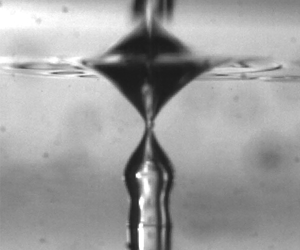
When a drop train collides with an initially unperturbed free surface of a liquid pool, a cavity starts to grow in the longitudinal direction, as shown in figure 2(a). Upon reaching a depth 20–150 times the diameter of the impacting drop, the slender cavity experiences pinch-off at a neck near the free surface, figure 2(b). The sealed air cavity breaks up into tiny air bubbles under the action of capillarity. The upper part of the cavity in a funnel shape (indicated in figure 2b) shrinks with time as its cusp ascends toward the free surface. Then the cavity assumes a steady-state shape except for a central region subjected to a continuous impact of drops, as shown in figure 2(c). The incoming drops afterwards merely penetrate the funnel to generate air cavities.
Temporal evolution of the cavity formed by the impact of 30 wt $\%$ ethanol (liquid IV) drops on a pool of the same liquid with d = 270 $\mathrm {\mu }$m, $f=18$ kHz and $U=7.6$ m s $^{-1}$. (a) Elongated cavity at $t=3.6$ ms with a magnified image of the tip crater. (b) Pinch-off of the neck of the cavity at $t=6.3$ ms. (c) Steady funnel and air bubbles at $t=116$ ms with a magnified image of the funnel. (d) The depth of the cavity, $H$, versus time, $t$.
$t$.

Such evolution of the cavity with impact of a drop train can be simply quantified as in figure 2(d), where the distance of the apex of the cavity from the unperturbed interface,  $H$, is plotted with time. Upon pinch-off of the elongated cavity near $t=7$ ms, $H$ drops rapidly corresponding to the formation of a funnel, whose depth reaches a constant value after $t\approx 15$ ms. We theoretically model the profile of the elongating cavity in this section, and rationalise the constant topography of the funnel in the next section.
3.1. Growth of tip crater
The growth of a cavity is an accumulative result of the successive creation of unit craters arising from impacts of individual drops, as can be seen through the striations of the elongated cavity in figure 2(a). Hence, we start our analysis with the evolution of a crater forming at the tip of the cavity by the impact of a single drop, referred to as a tip crater henceforth. As shown in figure 3(a), the impact of a single drop onto a liquid pool generates a crater which resembles a cylinder in the early stages but turns hemispherical afterwards (Fedorchenko & Wang Reference Fedorchenko and Wang2004). The hemispherical growth of the crater, which begins after  $t=5$ ms in figure 3(a), follows the power law, $h=R\sim t^{2/5}$ with $h$ and $R$ being the depth and radius of the crater, respectively. Leng (Reference Leng2001) rationalised this power law by balancing the kinetic energies of the impacting drop and the liquid surrounding the growing crater. In our experiments with drop trains, however, it takes only $1/f\in (1 - 300)\ \mathrm {\mu }$s for the tip crater to grow before the arrival of the next drop. Thus, the crater tip assumes a cylindrical, rather than hemispherical, shape, consistent with the magnified image in figure 2(a).
(a) The depth ( $h$) and the radius ( $R$) of a crater versus time after a single water drop impact on an unperturbed free surface. The diameter and impact velocity of the drop are respectively 4.5 mm and 3.3 m s $^{-1}$. (b) The experimentally measured temporal evolution of the depth of tip craters formed by the impact of the tenth drop in each experiment. (c) The depth of tip craters plotted according to the theoretical model, (3.3). (d) Experimental conditions for symbols in (b) and (c).

To find the temporal evolution of the depth of the tip crater,  $h$, we consider the momentum conservation for a cylindrical control volume (CV) surrounding the impacting drop as shown in figure 4(a,b). The velocity of the drop upon colliding with the liquid (at the cavity tip) is denoted as $u$. The CV moves with the interface between the drop and the liquid, and its velocity is $v$. The optically identifiable tip location corresponds to the red dot on the side of the CV, as indicated in figure 4(b). We assume that the crater tip moves with the CV, so that $v\simeq \mathrm {d}h/\mathrm {d}\tau$. Here, $\tau$ is the time measured from the collision of the drop with the elongating cavity, which should be discriminated from $t$, the time measured from the first impact of the drop train on an unperturbed liquid pool. For the CV moving with the time-varying velocity $v$, we write the $z$-directional momentum conservation equation for a non-inertial coordinate system accelerating with $\mathrm {d}v/\mathrm {d}\tau$:
 \begin{equation} \frac{\mathrm{d}}{\mathrm{d}\tau}[m(u-v)] =F-m\frac{\mathrm{d}v}{\mathrm{d}\tau}, \end{equation}
where  $m$ is the mass of the CV, and the external force acting on the CV is given by $F=-\rho A v^{2}$, with $\rho$ being the liquid density and $A$ the base area of the CV, under our assumption of inertia-dominant flow. Here, we ignored the $z$-directional momentum flux because the drainage from the impacting drop owing to the difference between $u$ and $v$ occurs dominantly in the $r$-direction (O $\tilde{g}$uz, Prosperetti & Kolaini Reference Og̃uz, Prosperetti and Kolaini1995; Bisighini et al. Reference Bisighini, Cossali, Tropea and Roisman2010). The mass drainage rate is given by $\mathrm {d}m/\mathrm {d}\tau =-\rho A(u-v)$. Then (3.1) becomes
 \begin{equation} m \frac{\mathrm{d}u}{\mathrm{d}\tau} = \rho A (u-v)^{2} - \rho A v^{2}. \end{equation}
(a) Schematic of an elongated cavity. A drop hitting the tip of the cavity generates a tip crater. (b) Schematic of a tip crater whose depth is indicated as  $h$. The colliding drop is coloured yellow. The control volume is represented with dashed lines. (c) Schematic of liquid flow with radial expansion of an elongated cavity. (d) Schematic of a funnel, whose depth $L$ is maintained constant despite continual impacts of drops. The cross-section of the funnel is illustrated in the box with the dashed lines.

We suppose that the discrepancy between  $u$ and $v$ cannot grow significantly during the brief growth of the tip crater, which allows us to write $u\approx v \approx \mathrm {d}h/\mathrm {d}\tau$. Then (3.2) is simplified to a differential equation for $h$:
$h$:  $\mathrm {d}^{2}h/\mathrm {d}\tau ^{2}+(\mathrm {d}h/\mathrm {d}\tau )^{2}/d=0$, where we used $\rho A/m\approx 1/d$. It is readily solved with the initial conditions of $h=0$ and $\mathrm {d}h/\mathrm {d}\tau =U$ at $\tau =0$, to give
 \begin{equation} \frac{h}{d} = \ln{\left( 1+\frac{U \tau}{d} \right)}. \end{equation}
We measured the tip crater depth versus time for various impact conditions and plotted the results in figure 3(b). The figure shows the experimental results for  $f<22$ kHz, which could be temporally resolved with the current high-speed camera. Still, the measurement duration is fairly short ( $\tau < 0.3$ ms) because of the quick arrival of the subsequent drop. Figure 3(c) shows that the scattered raw data in figure 3(b) are collapsed onto a single line with the slope of unity when plotted according to (3.3), which verifies our theoretical model. The vertical growth of tip crater gets faster with the increase of the drop diameter and impact velocity.
The growth of  $h$ with $\tau$ given in (3.3) allows us to obtain the maximum depth ( $h_0$) of the tip crater for each drop impact. The time interval between the impacts of two successive drops is given by ${\rm \Delta} t=1/f+h_0/U$. Substituting ${\rm \Delta} t$ for $\tau$ in (3.3) yields an equation for $h_0$:
 \begin{equation} \frac{h_0}{d}=\ln{\left(1+\frac{U}{fd}+\frac{h_0}{d}\right)}, \end{equation}
which can be solved numerically. We see that the maximum depth of a tip crater scaled by the drop diameter,  $h_0/d$, depends only on $\phi =fd/U$.
3.2. Growth of entire cavity
The entire depth of the elongated cavity,  $H$, at time $t$ measured from the first impact of drop is determined by superposing $h_0$ of all the previous tip craters. Thus, we write $H=h_0N$, where $N=t/{\rm \Delta} t$ is the number of drops that have arrived for the total time $t$. The elongation rate of the cavity can be expressed as $\dot {H}=\mathrm {d}H/\mathrm {d}t \approx h_0/{\rm \Delta} t$, so that the rate scaled by the drop impact velocity $U$ is given by
 \begin{equation} \frac{\dot{H}}{U} = \frac{\phi h_0/d}{1+\phi h_0/d}, \end{equation}
Because  $h_0/d$ is a function of $\phi$ in (3.4), $\dot {H}/U$ is also a function of $\phi$ only. Consequently, the depth of elongated cavity grows linearly with time.
Figure 5(a) plots our experimental data of the scaled elongation rate of the cavity as a function of  $\phi$ along with our theoretical result from (3.5). We have also included previously reported experimental data and theoretical prediction in the figure. Speirs et al. (Reference Speirs, Pan, Belden and Truscott2018) modelled the drop train as a continuous liquid stream rather than separate drops and balanced the pressures of the two media (pool and stream) at the stagnation point, to yield a simple relationship of $\dot {H}/U=\sqrt {\phi }/(1+\sqrt {\phi })$. We find that the experimental results using drop diameters of tens of micrometres (Bouwhuis et al. Reference Bouwhuis, Huang, Chan, Frommhold, Ohl, Lohse, Snoeijer and van der Meer2016), hundreds of micrometres (ours) and millimetres (Speirs et al. Reference Speirs, Pan, Belden and Truscott2018) follow the same trend. Both of the theoretical models predict the experimental results well, which confirms that the impact inertia of drops is dominantly converted to the momentum of the surrounding liquid.
(a) The scaled penetration speed of the elongated cavity,  $\dot {H}/U$, versus $\phi =fd/U$. The black solid line corresponds to (3.5), and the red dashed line to the model from Speirs et al. (Reference Speirs, Pan, Belden and Truscott2018). (b) The radius of a cavity $R$ at a fixed $z$ versus time, $\tau _r$. (c) The experimental cavity radius plotted according to (3.8). (d) The experimentally measured cavity profiles for various experimental conditions at $t=3$ ms. (e) The experimental cavity profile plotted according to (3.9), where $\psi$ is the right-hand side of (3.9). (f–h) Comparison of the experimentally imaged cavity shapes and the theoretical predictions given by the red line: (f) 30 wt% ethanol in water, d = 410 $\mathrm {\mu }$m, $U=10.6$ m s $^{-1}$ and $f=17$ kHz; (g) 4 wt% ethanol in water, d = 340 $\mathrm {\mu }$m, $U=9.4$ m s $^{-1}$ and $f=17$ kHz; (h) water, d = 430 $\mathrm {\mu }$m, $U=6.4$ m s $^{-1}$ and $f=7$ kHz. Experimental conditions for symbols in (a–e) are given in figure 3(d). The code and data necessary to plot (f–h) are available at https://github.com/Jay-JaeHongLee/JFMdroptrain.git.

We go beyond the mere prediction of the cavity depth, by analytically modelling the temporal evolution of the entire shape, i.e. radius as well as depth, of the cavity. We first consider the radial growth of each crater comprising the entire cavity. The crater formed by the drop impact at the cavity tip dominantly grows axially as a tip crater in the beginning, but it grows only radially once the next drop arrives to form a new tip crater. The radial expansion of the old crater implies the radially outward recession of the surrounding liquid as illustrated in figure 4(c). The corresponding kinetic energy of the liquid is written as
 \begin{equation} E_l={\rm \pi} \rho h_0\int^{R_\infty}_R rv_r^{2}\, \mathrm{d}r, \end{equation}
where  $R$ is the radius of the crater of interest at time $\tau _r$ measured from the moment it begins radial expansion, $R_\infty$ is a characteristic distance of the far field unaffected by the expansion of the crater and $v_r$ is the radial velocity of liquid at a distance $r$ from the centre of the cavity. Using the continuity equation, $v_r = R \dot {R} / r$ with $\dot {R} = \mathrm {d} R / \mathrm {d} \tau _r$, we find $E_l = {\rm \pi}\rho h_0 R^{2} \dot {R}^{2} \ln {(R_\infty /R)}$.
Because  $E_l$ comes from the kinetic energy of the impacting drop, $E_d={\rm \pi} \rho d^{3}U^{2}/12$, after a fairly brief period of tip crater formation, we estimate $E_l\sim E_d$, where $\sim$ signifies ‘is scaled as’:
 \begin{equation} \ln{\left( \frac{R_\infty}{R} \right)} \sim \frac{1}{12} \frac{d^{3} U^{2}}{h_0 R^{2} \dot{R}^{2}}. \end{equation}
Bouwhuis et al. (Reference Bouwhuis, Huang, Chan, Frommhold, Ohl, Lohse, Snoeijer and van der Meer2016) showed that the radius of the elongated cavity  $R\sim \tau _r^{1/2}$ via the two-dimensional Rayleigh equation. Then, $R^{2}\dot {R}^{2}$ is independent of time, and so is $\ln (R_\infty /R)$ approximately. Solving (3.7), we find
 \begin{equation} R^{2} =\frac{k dU}{(h_0/d)^{1/2}}\tau_r+R_0^{2}, \end{equation}
where  $k$ is a time-independent prefactor to be empirically determined, and $R_0$ is the initial radius of the cavity, which corresponds to the radius of the tip crater at the moment the next drop arrives.
Figure 5(b) shows the experimental results of the radius of a single crater (at fixed  $z$) versus time, $\tau _r$, for varying drop size, velocity, frequency and surface tension. The radius tends to increase rapidly in the initial stages but its growth slows down in the late stages, consistent with a power-law behaviour, $R \sim \tau _r^{1/2}$. We see in figure 5(c) that the scattered raw data are collapsed onto a single line when plotted according to our theoretical model, (3.8). The slope of the best fitting line by the least squares method gives $k=0.3$.
With the axial elongation and radial expansion of the cavity given by (3.5) and (3.8), respectively, we can reconstruct the temporal evolution of the cavity profile. The depth and radius of the cavity profile with its tip descending at a rate of  $\dot {H}$ are respectively given by $z=U \phi (h_0/d) \tau / [1+\phi (h_0/d)]$ from (3.5) and $r^{2} = kdU \tau _r /(h_0/d)^{1/2} +R_0^{2}$ from (3.8), where $\tau _r=\tau - {\rm \Delta} t$. Eliminating $\tau$ in the equations, we obtain an equation of the cavity profile:
 \begin{equation} \frac{z}{d} = \frac{\phi (h_0/d)^{3/2}}{k(1 + \phi h_0/d)}\frac{r^{2}-R_0^{2}}{d^{2}} + \frac{\phi h_0/d}{1 + \phi h_0/d} \left( \frac{1}{\phi} + \frac{h_0}{d} \right). \end{equation}
We can draw the cavity profile using (3.9) while the origin (the cavity tip) is descending at a rate given by (3.5). Two interesting observations follow (3.9). First, the parabolic profile of the elongated cavity is preserved as an observer travels with the cavity tip. Second, the profile depends only on  $\phi$ when the lengths ( $z$ and $r$) are scaled by the drop diameter $d$.
$d$.
In figure 5(d), we plot the measured cavity profiles for various experimental conditions including types of liquid, drop diameter and impact velocity. Figure 5(e) shows that the scattered raw data are collapsed onto a single line with the slope of unity, when plotted according to (3.9). We overlap the actual cavity images with the theoretical profiles in figure 5(f–h), to find their good agreement. The theoretical results tend to slightly overestimate the cavity radius as the maximum radius is approached before sealing because our model is based on the Rayleigh equation which considers only inertial expansion of the cavity.
4. Steady shape of funnel
Once the elongated cavity is sealed by necking near the unperturbed free surface, the cusp-shaped liquid–air interface above the pinch-off point retreats upward until it reaches a steady funnel shape, as shown in figure 2(c). Here, we theoretically model the steady profile of the funnel, which has rarely been discussed thus far, except for the air cavity around a liquid jet plunging into a liquid bath (Sheridan Reference Sheridan1966; Zhu, O $\tilde{g}$uz & Prosperetti Reference Zhu, Og̃uz and Prosperetti2000; Lorenceau & Quéré Reference Lorenceau and Quéré2004; Kiger & Duncan Reference Kiger and Duncan2012). Considering that the initial transient of elongated cavity formation and collapse takes less than 10 ms in our experiments, it is the steady funnel that is likely to play more important roles in practical applications.
As schematically illustrated in figure 4(d), the interfacial profile of the funnel arises as the downward force from the drop impact is balanced with the capillary forces. For the cylindrical control volume around the funnel, a dashed box in the figure, the drop impact force  $F_i$ is scaled as $F_i\sim \rho U^{2}d^{2}\phi$, where $\phi =fd/U$ has been included to account for the duration that the drop passes through the lower neck of the funnel ( $d/U$) relative to a period between successive drops ( $1/f$). The control volume is extended radially from the lower neck of funnel by the capillary length $l_c=[\sigma /(\rho g)]^{1/2}$, a characteristic length scale over which a static meniscus develops under the gravitational field. The vertical length of the control volume corresponds to the funnel depth $L$. The downward and upward capillary forces are respectively given by $F_d={\rm \pi} d\sigma$ and $F_u=2{\rm \pi} \sigma (r\sin \alpha ) |_{z=L}$ with $\sin \alpha =[(1+(\mathrm {d}r/\mathrm {d}z)^{2}]^{-1/2}$. We note that the vertical origin ( $z=0$) is positioned at $r = d/2$, the deepest point of the funnel. Balancing $F_i$ and $F_u-F_d$ with $r'=\mathrm {d}r/\mathrm {d}z\gg 1$ at $z=L$, we get
 \begin{equation} \frac{r}{r'}-\frac{d}{2} \sim \frac{1}{16}\phi d {We}. \end{equation}
Integrating (4.1) from  $z=0$ to $L$ and $r=d/2$ to $l_c$, we find a relationship between the funnel depth, $L$, and the drop train impact conditions:
 \begin{equation} \frac{L}{d}-\frac{1}{2}\ln\left(\frac{2l_c}{d} \right)\sim \frac{1}{16}\phi \textit{We} \ln{\left(\frac{2l_c}{d} \right)}. \end{equation}
 Figure 6(a) displays the experimental results of the funnel depth  $L$ versus the impact velocity $U$ of drops with various conditions. The funnel depth tends to increase with the impact velocity for drops with similar sizes (hundreds of micrometres in diameter) but are also sensitive to the drop size as seen in the lower right corner of the plot (d = 20 $\mathrm {\mu }$m). However, plotting the raw data according to (4.2) collapses them onto a single line, as shown in figure 6(b). Then we can write $L/d=\frac {1}{2}(1+c\phi {We}/8)\ln (2 l_c/d)$, with $c=0.015$. In figure 6, the results of the additional experiments have been included, where the atmospheric gas was substituted by SF $_6$ with a density five times greater than air (6.1 kg m $^{-3}$) to check the effects of the momentum of gas entrained with the drops. The agreement of the experimental results with our theoretical model confirms a negligible effects of entrained gas on the funnel shape.
(a) Experimental results of a funnel depth  $L$ versus the velocity of drops with varying conditions. (b) The data in (a) plotted according to (4.2). The slope of the best fitting line is 0.015. (c) Interfacial profiles of funnels for a range of drop train impact conditions. (d) The scaled profiles of funnel interface plotted according to (4.3), which are collapsed onto a straight line with the slope unity. (e–g) Experimental images of funnels formed by impact of drop trains: (e) water, d = 20 $\mathrm {\mu }$m, $U = 32.9$ m s $^{-1}$ and $f = 635$ kHz; (f) ethanol, d = 180 $\mathrm {\mu }$m, $U=4.6$ m s $^{-1}$ and $f = 14$ kHz; (g) ethanol, d = 220 $\mathrm {\mu }$m, $U=9.7$ m s $^{-1}$ and $f = 17.2$ kHz; ( $h$) water, d = 240 $\mathrm {\mu }$m, $U = 9.5$ m s $^{-1}$ and $f = 27.7$ kHz. The red lines correspond to the theoretical prediction (4.3), and they extend up to $r=l_c$ in (f–h).

Now we can obtain the meniscus profile of the funnel by integrating (4.1) from  $z=0$ to $z$ and $r=d/2$ to $r$:
$r$:
 \begin{equation} \frac{z}{d}=\frac{1}{2} \left(1+\frac{c}{8}\phi{We}\right)\ln\left(\frac{2r}{d}\right). \end{equation}
We see that the scaled funnel profile depends on  ${We}$ as well as $\phi$, unlike the elongated cavity that depends only on $\phi$, as seen in (3.9). Figure 6(c) plots interfacial profiles of the funnels for various experimental conditions. In figure 6(d), the scattered profiles are seen to collapse onto a single line when plotted according to (4.3). We further see in figure 6(e–g) that the theoretically predicted meniscus profiles match well with experimental images under different impact conditions. The funnel profiles corresponding to $r>d/2$ are kept steady despite interfacial oscillations arising from drop impacts in the inner region ( $r< d/2$).
5. Conclusions
We have theoretically modelled and experimentally corroborated the dynamic evolution of an elongated cavity that is formed by impact of a drop train on a liquid pool. Although the prior works obtained a scaling law for cavity elongation rate and numerically simulated the cavity shape, our model with experiments allows us to find the temporal evolution of the cavity profile in a closed form. We have also analysed the liquid interface profile, a funnel, which arises after the elongated cavity is collapsed owing to capillary action. The funnel geometry has been shown to depend on the Weber number as well as the dimensionless frequency  $\phi$.
Although the funnel has been largely ignored in the previous studies of a drop train impact, it is indeed one of the most important interfacial phenomena that discriminates the impact of a drop train from relatively scattered impacts of drops onto a liquid pool (Bick et al. Reference Bick, Ristenpart, van Nierop and Stone2010; Ray et al. Reference Ray, Biswas, Sharma and Welch2013). Although such a funnel was observed when a liquid jet plunges into a liquid pool, the effects of jet inertia on the steady shape of the funnel have been rarely considered because major attention has rather been paid to air entrainment behaviour arising from jet impacts (Sheridan Reference Sheridan1966; Zhu et al. Reference Zhu, Og̃uz and Prosperetti2000; Lorenceau & Quéré Reference Lorenceau and Quéré2004; Kiger & Duncan Reference Kiger and Duncan2012). In practice, understanding the fields of flow and pressure around the elongated cavity and funnel is essential in designing effective semiconductor cleaning processes. For such applications, it is worth further investigation to elucidate how the kinetic energy of the incoming drops is transferred within a liquid to dislodge contaminant particles attached to the bottom surface.
Funding
This work was supported by National Research Foundation of Korea (Grant No. 2018052541) via SNU IAMD.
Declaration of interests
The authors report no conflict of interest.


 Open access