


1. INTRODUCTION
The Quaternary period, spanning the last 2.6 million years of Earth history, was marked by warm and short interludes between long and cold periods. While literature provides tight constraints on how climate varied during glacial periods in marine settings (Zachos and others, Reference Zachos, Pagani, Sloan, Thomas and Billups2001; Lisiecki and Raymo, Reference Lisiecki and Raymo2005; Herbert and others, Reference Herbert2016), changes in temperature and precipitation on continents remain poorly constrained. Use and availability of proxies such as pollen (Peyron and others, Reference Peyron1998) and speleothems (Luetscher and others, Reference Luetscher2015) can help shed more light on past climate conditions. However, past glacial advances have left a strong imprint on the Earth's surface in the form of moraines, trimlines and other glacial geomorphic features, which provide us invaluable information on past climate on continents (Penck, Reference Penck1905; Plummer and Phillips, Reference Plummer and Phillips2003; Laabs and Carson, Reference Laabs and Carson2005). Furthermore, thanks to geochronological methods (Gosse and Phillips, Reference Gosse and Phillips2001), such as14C (Hajdas, Reference Hajdas2009), cosmogenic nuclide (Blanckenburg and Willenbring, Reference Blanckenburg and Willenbring2014) and optically stimulated luminescence dating (Rhodes, Reference Rhodes2011), the timing of past glacial advances can be dated.
Ice-flow models have been used before to infer past climate conditions on continents (Plummer and Phillips, Reference Plummer and Phillips2003; Anderson and others, Reference Anderson, Molnar and Kessler2006; Kessler and others, Reference Kessler, Anderson and Stock2006; Jouvet and others, Reference Jouvet, Picasso, Rappaz and Blatter2008; Golledge and others, Reference Golledge2012; Rowan and others, Reference Rowan, Brocklehurst, Schultz, Plummer, Anderson and Glasser2014; Eaves and others, Reference Eaves, Mackintosh and Anderson2016; Mey and others, Reference Mey2016). These studies consisted of running ice-flow models forward and fitting observed moraines by optimizing some of the model parameters. A key component in such models is the mass balance, which defines ice accumulation and ablation, and is thus primarily a function of precipitation and temperature (Cuffey and Paterson, Reference Cuffey and Paterson2010). Several models exist to simulate mass balance, from the simple positive degree-day model (Braithwaite, Reference Braithwaite1995) to more sophisticated energy mass-balance models (Oerlemans, Reference Oerlemans1992, Reference Oerlemans1997; Becker and others, Reference Becker, Seguinot, Jouvet and Funk2016; Pellicciotti and others, Reference Pellicciotti2016). These models have been successfully applied to reconstruct glacial history (Becker and others, Reference Becker, Seguinot, Jouvet and Funk2016; Seguinot and others, Reference Seguinot2018), but require knowledge of a large number of uncertain parameters, which might change over a glacial cycle. In-depth analysis of ice-flow models used for paleoclimatic reconstructions can be found in the paper by Kirchner and others (Reference Kirchner2016).
In practice, past ice thicknesses are poorly constrained. Recent studies on the European Alps have emphasized the systematic mismatch between paleo ice-flow model and reconstruction from trimlines (e.g., Cohen and others, Reference Cohen, Gillet-Chaulet, Haeberli, Machguth and Fischer2017; Seguinot and others, Reference Seguinot2018), in terms of ice thickness. Here we introduce an inversion method to infer spatially varying mass-balance information from the former extent of glaciers derived from geomorphological observations, such as moraines. We apply a gradient descent method to minimize a cost function, which includes the misfit between modeled and geomorphological maximal glacial extents and a regularization term to ensure sufficient smoothness of the inverted variables. As a result, the method consists of running a forward model a large number of times with a tuning of the mass balance at each iteration. The ice-flow model is modeled by solving the mass conservation equation using the shallow ice approximation (SIA) (Mahaffy, Reference Mahaffy1976; Hutter, Reference Hutter1983) and the developed codes are accelerated using Graphic Processing Units (GPUs).
Below, we first introduce the basic equations governing our forward model. Then we present the theoretical basis behind the method and provide a step-by-step recipe for its numerical implementation. We then illustrate the method's efficiency for constraining spatial variations in mass balance over mountain ranges with a series of examples.
2. FORWARD MODEL
2.1. Ice dynamics
At the time scale relevant for ice-sheet dynamics, ice can be described as a viscous and incompressible non-Newtonian fluid (Cuffey and Paterson, Reference Cuffey and Paterson2010). Ice thickness can be modeled by solving the mass conservation equation:
 $$\displaystyle{{\partial H} \over {\partial t}} =- \nabla \cdot {\bf q} + b,$$
 where H is the ice thickness, q is the horizontal ice flux and b represents the mass-balance rate. Horizontal ice flux is defined as vertically integrated velocity field  ${\bf q} = \int _{B}^{S}{\bf u}\,{\rm d}z$, and we approximate velocities using the SIA:
 $$ \eqalign{{\bf u}(z) &= -\underbrace{A (\rho g)^n [H^{n+1} + (S - z)^{n+1}] |\nabla S|^{n-1} \nabla S}_{\it (i)} \cr &\quad + \underbrace{A_s (\rho g)^n H^{n-1} |\nabla S|^{n-1} \nabla S }_{\it (ii)}, $$
where (i) represents the deformation velocity and (ii) represents the sliding velocity, S is the surface altitude, ρ is density of ice, g is the gravitational acceleration, A is the ice-flow parameter, A s is a sliding parameter and n is the Glen flow law exponent. Values for the flow parameters A and A s are taken from Oerlemans (1997) (who used values from Budd and others (Reference Budd, Keage and Blundy1979)), and can be found listed in Table 1, along with the other parameter values used in the model.
Ice-flow model parameters
The SIA is based on the assumption that large ice bodies are mainly deformed by vertical shear stress, and therefore neglects longitudinal stresses in the mass conservation equation (Eqn 1). We are using this approximation with the assumption that the horizontal scale of the ice extent is much larger than the vertical scale (H ≪ L). Solving of full set of Stokes equations, a full set of momentum equations, would give more realistic results (especially near the margin and ice divide). However, the ice extent is primarily a function of mass balance, topography and ice dynamics. Since we only consider the extent of ice as forward model output in our inversion method, we restrict our analysis to the SIA.
The mass-balance rate, b, is defined as the annual gain, accumulation, or loss of mass, ablation, at the glacier surface (e.g., Oerlemans, Reference Oerlemans2001; Cuffey and Paterson, Reference Cuffey and Paterson2010). We define the mass-balance rate, b, as a spatially varying variable:
 $$ b=\min(\beta (S(x,y)-E(x,y)),c), $$
where β is the balance rate gradient, E is the equilibrium line altitude (i.e., the location where accumulation is equal to ablation) and c is a maximum ice accumulation rate (e.g., Meier, Reference Meier1962; Kessler and others, Reference Kessler, Anderson and Stock2006; Oerlemans, Reference Oerlemans2008). The evolution of the ice cap or glacier surface is in part determined by the mass-balance rate and its values depend on the local climate conditions. Mass-balance rate is positive in the accumulation area and negative in the ablation area. The mass-balance gradient, β, tends to be steeper in the ablation than accumulation area (Mayo, Reference Mayo1984). To keep the problem simple for introducing the inversion method, we choose the balance gradient to be constant.
Solving Eqn (1) using the SIA (Mahaffy, Reference Mahaffy1976; Hutter, Reference Hutter1983) leads to a non-linear diffusion-reaction type equation that can be solved numerically (Hindmarsh and Payne, Reference Hindmarsh and Payne1996). In that case, the ice flux q is defined as
 $${\bf q}=-D\nabla{S}, \quad S=H+B, $$
where B is the bedrock and D is the diffusivity expressed as:
 $$D=(\rho g)^n[AH^{n+2} + A_{\rm s}H^n]\vert \nabla{S} \vert^{(n-1)}. $$
The main advantage of models based on using SIA to solve the mass conservation equation Eqn (1) is their computational efficiency, which we further enhance using GPUs. The details of the numerical implementation we use can be found in the Appendix A. Note, however, that the inversion method approach we propose can be used with other types of approximations for ice flow, such as solving a full set of Stokes equations or a higher order approximation of these equations (e.g., Pattyn, Reference Pattyn2003; Egholm and others, Reference Egholm, Knudsen, Clark and Lesemann2011), as long as it is computationally possible. For the moment, running 1000–3000 inversion model runs with higher order models without the use of GPUs is not practical.
3. INVERSION METHOD
In this section, we provide the theoretical basis of the inversion method and its numerical implementation.
3.1. Theoretical basis
Our objective is to invert a known ice extent into a spatially variable E using the forward model explained in Section 2. The forward problem is defined as:
 $$h_{\rm m}(x,y) = F(E(x,y),\beta), $$
where h m(x, y) is the data we are trying to fit (note that h(x, y) is used for ice extent and H(x, y) for ice thickness), F is the forward model (the ice-flow model), and E(x, y) and β are the unknown parameters of the mass-balance equation, Eqn (3), we wish to constrain. Below we derive the method to infer E(x, y) and show it can be extended to β.
As with any inversion method, the primary objective is to minimize the misfit between the model predictions and the observations. To do so, we define a misfit function G(E) as a spatially integrated difference between the ice extent calculated for a forward model, h m(x, y), and the observations, h o(x, y) as:
 $$G(E) = \displaystyle{1 \over 2}\int_0^{L_x} {\int_0^{L_y} {(h_{\rm o}(} } x,y)-h_{\rm m}(x,y))^2{\rm d}x{\rm d}y,$$
where [0, L x] × [0, L y] is our computational domain. The chosen computational domain strictly contains the area where thickness is positive, i.e., we have S = B in the neighborhood of the border of the domain. The goal is then to minimize the misfit function G by varying E(x, y) iteratively.
We now look for a descent direction to define a sequence of E i, which minimizes the misfit function G. For that purpose, we formally compute 〈G′(E), δE〉, the directional derivative of G with respect to E along a given direction δE:
 $$\left\langle {{G}^{\prime}(E),\delta E} \right\rangle = -\int_0^{L_x} {\int_0^{L_y} {(h_{\rm o}(} } x,y)-h_{\rm m}(x,y))\displaystyle{{\partial h_{\rm m}(x,y)} \over {\partial E}}\delta E{\rm d}x{\rm d}y.$$
The term ∂h m/∂E represents the change of ice extent with respect to E, which are both function of x and y.
The goal of the inversion is to minimize G, and thus make 〈G′(E), δE〉 negative. However, the inverse problem is underdetermined (Hansen, Reference Hansen1994; Zhang and Xu, Reference Zhang and Xu2011). We solve this by imposing some form of regularization. Here we assume a smooth solution and impose smoothness on E using a Tikhonov regularization (Tikhonov, Reference Tikhonov1963; Poplavskii and others, Reference Poplavskii, Podladchikov and Stephenson2001). We do this by defining a new misfit function G, now containing the regularization term:
 $$\eqalign{G(E) &= \displaystyle{1 \over 2}\int_0^{L_x} {\int_0^{L_y} \bigg[ } \underbrace{{{(h_{\rm o}(x,y)-h_{\rm m}(x,y))}^2}}_{{(i)}} \cr & \quad + \underbrace{{\tau _2 \bigg[{\bigg(\displaystyle{{\partial E} \over {\partial x}}\bigg)}^2 + {\bigg(\displaystyle{{\partial E} \over {\partial y}}\bigg)}^2}}_{{(ii)}}\bigg]\bigg]{\rm d}x{\rm d}y,}$$
(i) in Eqn (9) is the same as in Eqn (7), while (ii) imposes the smoothness on the solution. The parameter τ 2 is a positive constant which acts as the additional constraint of smoothness. A large constant would force the solution to be very smooth, while a small or zero constant would cancel this constraint. Following the same derivation as above for (ii):
 $${ \left\langle {{G}^{\prime}(E),\delta E} \right\rangle = \int_0^{L_x} {\int_0^{L_y} {\tau _2} } \left( {\displaystyle{{\partial E} \over {\partial x}}\displaystyle{\partial \over {\partial x}}\delta E + \displaystyle{{\partial E} \over {\partial y}}\displaystyle{\partial \over {\partial y}}\delta E} \right){\rm d}x{\rm d}y,$$
and using the integration by parts:
 $$\eqalign{& \int_0^{L_x} {\int_0^{L_y} {\left[ {\displaystyle{{\partial E} \over {\partial x}}\displaystyle{\partial \over {\partial x}}\delta E + \displaystyle{{\partial E} \over {\partial y}}\displaystyle{\partial \over {\partial y}}\delta E} \right]} } \,\;{\rm d}x{\rm d}y \cr & \quad = \left[ {\left( {\displaystyle{{\partial E} \over {\partial x}} + \displaystyle{{\partial E} \over {\partial y}}} \right)\delta E} \right]_{0,0}^{L_x,L_y} {\rm -}\int_0^{L_x} {\int_0^{L_y} {\left( {\displaystyle{{\partial ^2E} \over {\partial x^2}}\delta E + \displaystyle{{\partial ^2E} \over {\partial y^2}}\delta E} \right)} } \,{\rm d}x{\rm d}y.} $$
Because the first term on the right-hand side becomes negligible, as there is no ice on the boundaries of the model, we can choose E in the neighborhood of the border such that ∂E/∂x = ∂E/∂y = 0, so 〈G′(E), δE〉 becomes:
 $$\left\langle {{G}^{\prime}(E),\delta E} \right\rangle = \int_0^{L_x} {\int_0^{L_y} {\left[ {-\tau _2\left( {\displaystyle{{\partial ^2E} \over {\partial x^2}} + \displaystyle{{\partial ^2E} \over {\partial y^2}}} \right)} \right]} } \delta E{\rm d}x{\rm d}y,$$
which combined with Eqn (8) gives:
 $$\eqalign{\left\langle {G^{\prime}(E),\delta E} \right \rangle & = \int_0^{L_x} {\int_0^{L_y} {\left[ {\left( {h_{\rm o}(x,y)-h_{\rm m}(x,y)} \right)\left( {-\displaystyle{{\partial h_{\rm m}(x,y)} \over {\partial E}}} \right)} \right.} } \cr & \quad \left. {- \; \tau _2\left( {\displaystyle{{\partial ^2E} \over {\partial x^2}} + \displaystyle{{\partial ^2E} \over {\partial y^2}}} \right)} \right]\delta E{\rm d}x{\rm d}y.} $$
Following the same logic, one can perform the same development for β instead of E:
 $$\eqalign{\left\langle {G^{\prime}(\beta ),\delta \beta } \right\rangle & = \int_0^{L_x} {\int_0^{L_y} {\left[ {\left( {h_{\rm o}(x,y)-h_{\rm m}(x,y)} \right)\left( {-\displaystyle{{\partial h_{\rm m}(x,y)} \over {\partial \beta }}} \right)} \right.} } \cr & \quad \left. {- \; \tau _2\left( {\displaystyle{{\partial ^2\beta } \over {\partial x^2}} + \displaystyle{{\partial ^2\beta } \over {\partial y^2}}} \right)} \right]\delta \beta {\rm d}x{\rm d}y.} $$
3.2. Numerical implementation of the inverse algorithm
To this end, we use the gradient descent method (Press, Reference Press2007; Fletcher, Reference Fletcher2013), in which E(x, y) is updated with the following increment:
 $$\delta E = -\left[ {\tau _1\left( {h_{\rm o}-h_{\rm m}} \right)-\tau _2\left( {\displaystyle{{\partial ^2E} \over {\partial x^2}} + \displaystyle{{\partial ^2E} \over {\partial y^2}}} \right)} \right].$$
This choice of δE leads to a decrease of the misfit G, assuming an appropriate choice of the iteration parameters τ 1 and τ 2, which are positive constants. We show below that recombining and substituting Eqn (15) into Eqn (13) results in negative increment of the misfit G:
 $$\eqalign{\left\langle {G^{\prime}(E),\delta E} \right\rangle & = \int_0^{L_x} {\int_0^{L_y} {\left[ {-\delta E-\left( {h_{\rm o}(x,y)-h_{\rm m}(x,y)} \right)} \right.} } \cr & \quad\times \left. {\left( {\displaystyle{{\partial h_{\rm m}(x,y)} \over {\partial E}} + \tau _1} \right)} \right]\delta E{\rm d}x{\rm d}y.} $$
Sorting Eqn (16) leads to:
 $$\eqalign{\left\langle {{G}^{\prime}(E),\delta E} \right\rangle &= -\int_0^{L_x} {\int_0^{L_y} {{\left[ {\delta E} \right]}^2} } {\rm d}x{\rm d}y \cr &\quad -\int_0^{L_x} {\int_0^{L_y} {\left( {h_{\rm o}(x,y)-h_{\rm m}(x,y)} \right)} } \cr & \quad \times\left( {\displaystyle{{\partial h_{\rm m}(x,y)} \over {\partial E}} + \tau _1} \right)\delta E{\rm d}x{\rm d}y.}$$
One can see that Eqn (17) is negative if the term (h o(x, y) − h m(x, y)) is sufficiently small, in other words the method converges if our initial guess is not too far from the final solution.
In practice, we follow the steps of the inversion algorithm presented in Table 2. First, we start by assigning an initial guess for E (step I). We arbitrarily choose an equilibrium line altitude field, E, and add some white noise to avoid imposing a spatial pattern to the solution, and therefore avoid the influence of the initial guess on the solution. Adding random noise enables to test whether the method can retrieve a meaningful solution or not, even with a poor initial guess. Next, the mass conservation equation Eqn (1) is solved using the mass-balance rate field, (b), calculated using the input E, Eqn (3), and the model is run until a steady state is reached, i.e., the ice thickness and ice extent do not change (step II). The output of the forward model, i.e., the ice extent, is used to calculate γ (step III). We define γ as the difference between observed ice extent data and ice extent calculated from a forward model run. Note that although the algorithm works using ice thickness (H), we rarely know it. In that case, we calculate ice extent (h) by setting ice thickness equal to 1 where there is ice, and equal to 0 where there is no ice. Step IV consists of updating the equilibrium line altitude locally by increasing (or decreasing) it where the modeled ice extent/ice thickness was found large (or small). If the glacier is too thick or goes beyond the ice extent, E is raised. Conversely, E is lowered if the glacier extent is too small. We then regularize the problem by applying diffusion on E using τ 2 (step V) for a chosen number of diffusion iterations, n sm. Steps IV and V correspond to one step of the descent direction given by Eqn (15). Finally, we return to step II, and iterate until γ is minimized (step VI). In the case where we want to invert for β instead of E, the described steps remain the same. One only needs to replace E with β in the equations since the equations are identical.
Implementation of the inversion algorithm
The parameters τ 1 and τ 2 are positive scalar values, which must be chosen. Both τ 1 and τ 2 are problem dependent. The choice is based mainly on the spatial dimensions of the problem and the spatial variability of the solution.
Furthermore, the choice of the inversion update parameter τ 1 reflects on the precision of the result. Too high a value will make it difficult for the inversion algorithm to converge to the solution because of too large jumps in value of E after each inversion step. On the other hand, a small value, after applying diffusion, might not result in a change in E that is sufficiently large enough to modify the ice extent of an area, thus not enable to fit the data successfully.
Diffusion in step V represents the smoothness one wishes to impose on E. We do this by iteratively solving the diffusion equation using a fully explicit scheme. The degree of smoothness is set by the number of iterations used in the explicit scheme. A large number of diffusion iterations may lead to a very smooth solution, and might not enable to capture local variations in mass-balance rate. In contrast, a small number of diffusion iterations leads to overfitting the data. We must keep in mind that we are fitting the ice extent by varying only one physical parameter, E, and that differences between observations and our model output could come also from the assumptions made in our forward model. The choice of number of diffusion iteration is illustrated later on.
We would like to stress here, the algorithm shows that the method only requires computing ice thickness and the Laplacian of E.
4. RESULTS
In this section, we illustrate the efficiency of the method with a series of synthetic examples. We start with a simple 2-D problem and then present a 2-D synthetic example using real topography (Uinta Mountains). In the simple 2-D example we show, in separate experiments, that the method can invert the ice extent in order to recover both E and β, while in the Uinta Mountains example we show that one can use ice thickness as well as ice extent to reconstruct E. Finally, we show how the method can be applied to a natural example at the Last Glacial Maximum (LGM) in the South Island of New Zealand. In the following experiments, ice extents are presumed to be reached at the same time, steady state solution, and sliding is parametrized to be constant. The balance gradient, β, is also kept constant in all examples except where we use the method to recover β. Since we can only do our inversion in the area of the map where we have ice, the results will also be presented only within the ice extent.
4.1. Two-dimensional inversion
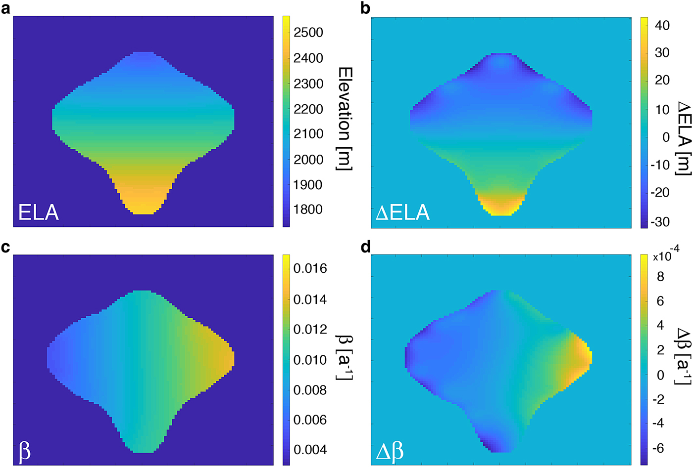
For this 2-D case, we present two experiments. First, we invert the synthetic ice extent and assess whether the method enables us to recover the prescribed E, and in the second experiment we show that the method is capable to recover β as well. The ice thickness, hence ice extent as well, are simulated by prescribing an arbitrary E and β.
A combination of two simple Gaussian shapes is used for the bedrock:
 $$B = B_0\left[ {\exp \left( {-\displaystyle{{X^2} \over {{10}^{10}}}-\displaystyle{{Y^2} \over {{10}^9}}} \right) + \exp \left( {-\displaystyle{{X^2} \over {{10}^9}}-\displaystyle{{(Y-(L_y/8))^2} \over {{10}^{10}}}} \right)} \right],$$
where B 0 is the maximum bedrock elevation, X and Y represent the matrices of distance vectors, and L y is the length scale in the y-direction. The prescribed E o we wish to recover is defined as follows:
 $$E_{\rm o} = 2150 + 900\arctan \left( {\displaystyle{Y \over {L_y}}} \right).$$
In this experiment, β is constant and set to 0.01. The initial guess is equal to 3000 m with 400 m amplitude white noise.
In the second experiment, we show that the method enables to recover the mass-balance gradient, β. For this, we use the same setup as above, i.e., bedrock is defined as in Eqn (18), and E as in Eqn (19). We prescribe β o we wish to recover:
 $$\beta _{\rm o} = 0.01 + 0.015\arctan \left( {\displaystyle{X \over {L_x}}} \right),$$
where L x is the length scale in the x-direction.
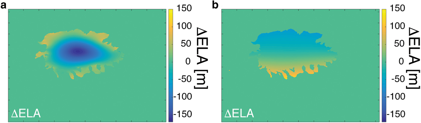
Figure 1 shows the calculated E and β (Figs 1a and 1c) and the differences between our inversions and the prescribed values (Figs 1b and 1d). In both cases, during the inversion, convergence is reached when the differences between the forward model output ice extent differ from our synthetic ‘observations’ by <10 points. The results show that convergence is reached after 293 iterations for E and 149 iterations for β. More importantly, the two results demonstrate that it is possible to recover E and β using this approach, and capture the spatial variation that was imposed by Eqns (19) and (20) and illustrated in Figs 1a and 1c. The parameters used in this test are summarized in Table 3.
(a) shows the calculated (modeled) E using our inversion algorithm, (b) difference between synthetic and calculated E where there is ice (within the ice extent), (c) shows the calculated (modeled) β using our inversion algorithm, (d) difference between synthetic and calculated β where there is ice (within the ice extent).
Two-dimensional inversion parameters
4.2. Two-dimensional inversion, Uinta Mountains synthetic test
Now the method is applied to a real topography. In this example, we show that the method is capable of restoring spatially variable E by using the ice extent as well as ice thickness as data. The Uinta Mountains, North America, was used as bedrock topography (Fig. 2a). The topography was extracted from the SRTM data (Jarvis and others, Reference Jarvis, Reuter, Nelson and Guevara2008) and smoothened using a median filter.
(a) shows the bedrock map used (Uinta Mountains) with the synthetic ice extent, (b) is the calculated (modeled) E using our inversion algorithm, (c) difference between synthetic and calculated E where there is ice (within the moraines extent).
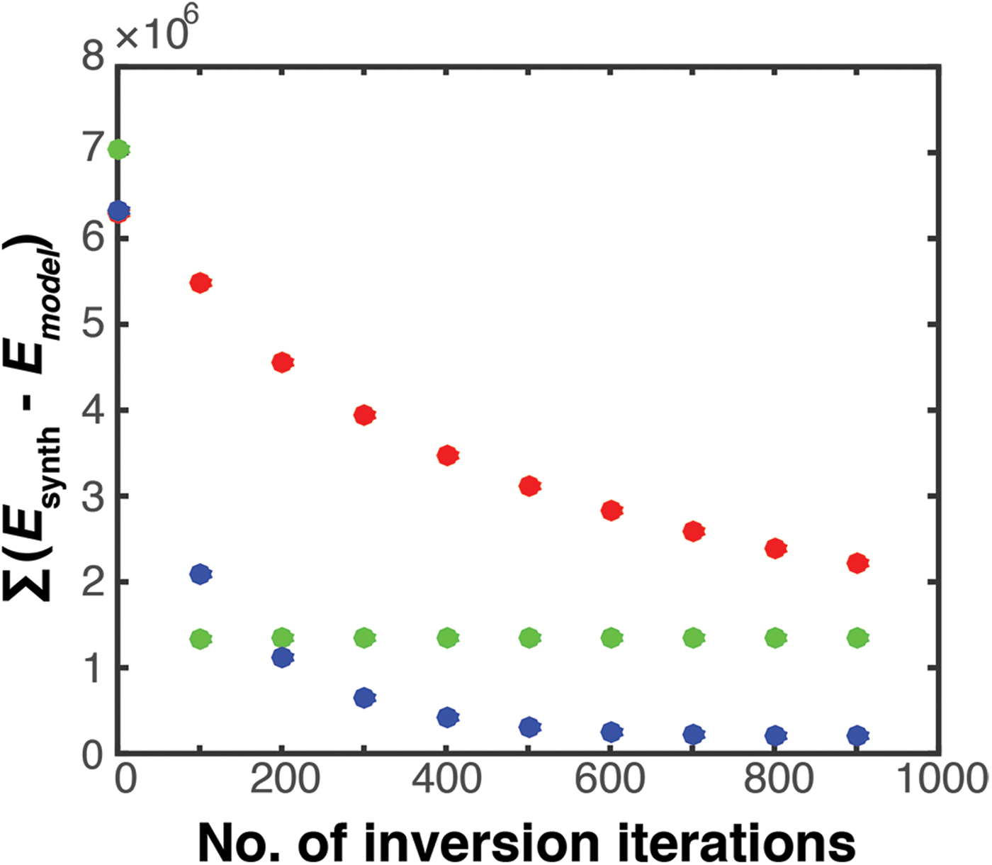
First, a forward model was run with a prescribed E o, which includes some spatial variability. The imposed pattern follows a N–S arctangent form. The ice extent is derived from the calculated ice thickness, which then represents the synthetic observations that we wish to invert for mass balance. The ice extent is calculated by setting the ice thickness equal to 1 where there is ice, and to 0 where there is not. Furthermore, high peaks that pierce through the ice are not included in our misfit calculations. The initial guess for E m field is 3100 m with 400 m amplitude random white noise added to it. To assess the performance of the inversion scheme, the sum of differences between the synthetic E o field and the calculated E m are monitored. All parameters used can be found in Table 4.
Uinta Mountains inversion experiment parameters
The results of the inversion for the E m field are presented in Fig. 2. The differences between the prescribed solution E o and inversion model solution E m are <30 m, which falls under 5% difference from the prescribed solution (Fig. 2c).
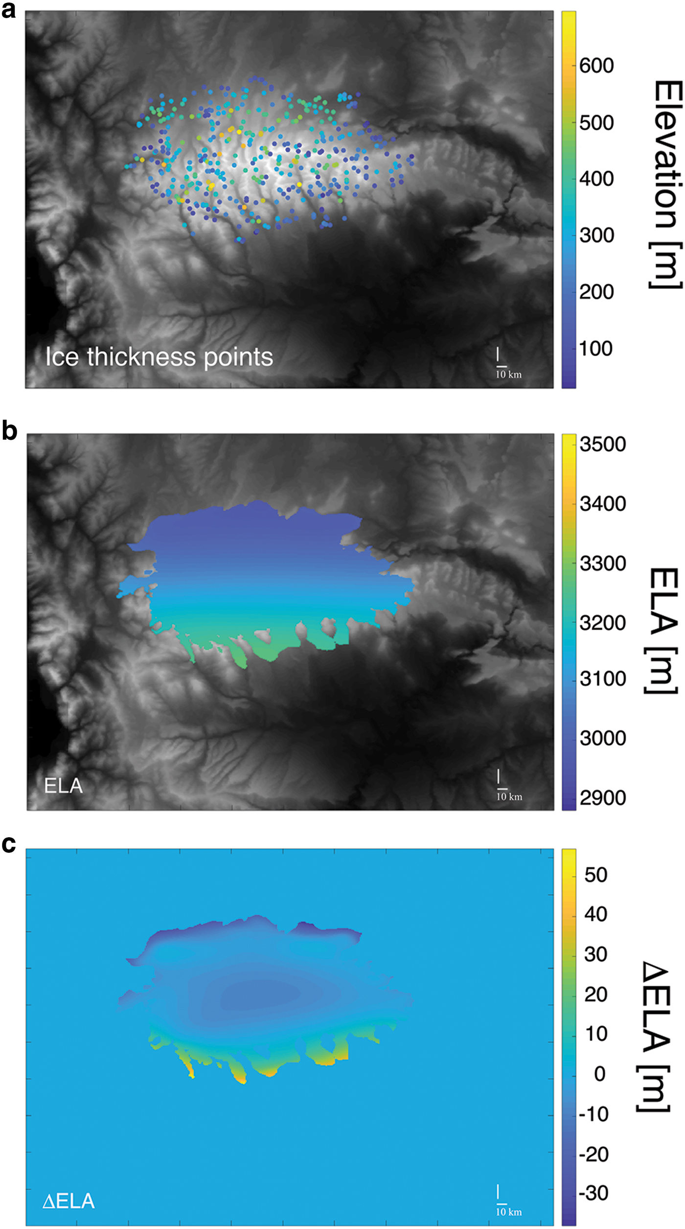
We now repeat the same test with the same forcing, but instead of using the ice extent we randomly chose ice thickness points on our synthetic glacier. Out of 40 317 ice thickness points within the ice extent we chose 433 (Fig. 9a). The only difference in the approach from the previous example is that now we calculate γ as a difference of ice thickness values in the chosen points between calculated and synthetic ice. The resulting figures (Fig. 9 in Appendix B) and tables with used parameters can be found in Appendix B.
Now we investigate the influence of the number of the diffusion iterations. We report two different end-member cases. The first one uses only five diffusion iterations (Fig. 3a) and the second uses 5000 iterations (Fig. 3b). Fig. 3 shows the differences between the E o for the two end-member tests. It appears that the choice of the number of diffusion iterations strongly influences the precision of the result. A large number of diffusion iterations reduces the spatial variability in mass balance, and is thus filtering out any local gradient, whereas a small number of diffusion iterations reduces the rate at which the residuals are decreased (Fig. 4).
(a) is the difference between synthetic and calculated E where there is ice ( within the moraines ice extent) with number of diffusion iterations set to 5, (b) is the difference between synthetic and calculated E where there is ice with number diffusion of iterations set to 5000.

4.3. Inversion of LGM ice extent in the South Island of New Zealand
To verify the method for a real situation, we reconstruct the LGM mass balance using the observed ice extent of the South Island of New Zealand (Barrell, Reference Barrell2011). This example offers us the possibility of comparing the results with previous reconstructions (Golledge and others, Reference Golledge2012).
The South Island's climate is heavily influenced by the Westerlies. As the air flows across the Southern Alps, precipitation is orographically enhanced with up to 10 m a−1 of precipitation on the west side (Henderson and Thompson, Reference Henderson and Thompson1999). The eastern slopes see considerably lower rates of precipitation (about 1 m a−1) as a consequence of the westerly airflow across the mountain range.
In the past, the Southern Alps have experienced extensive glaciations, including full transitions from glacial to fluvial processes (Whitehouse, Reference Whitehouse1988). Climate has controlled the growth and decay of mountain glaciers in New Zealand since at least 2.4–2.6 Ma (Suggate, Reference Suggate1990), as testified by an exceptional moraine record across the entire South Island (Barrell, Reference Barrell2011). During the LGM, the North Atlantic meridional overturning circulation was weakened compared with present, the Intertropical Convergence Zone shifted southward, which in the southern mid-latitudes modified the location of wind and temperature (Rojas and others, Reference Rojas2009; Denton and others, Reference Denton, Anderson and Toggweiler2010; McGlone and others, Reference McGlone, Turney and Wilmshurst2010). The LGM was thus marked by changes in regional atmospheric conditions that affected winds and precipitation in the Southern Alps, which may have led to a change in humidity, possibly up to 25% drier than today (Golledge and others, Reference Golledge2012). Temperatures were between 4°C and 8°C lower than today (Newnham and others, Reference Newnham, Lowe and Green1989; Barrows and others, Reference Barrows, Juggins, De Deckker, Calvo and Pelejero2007; Golledge and others, Reference Golledge2012; Seltzer and others, Reference Seltzer, Stute, Morgenstern, Stewart and Schaefer2015). Most importantly, despite these changes, the orographically enhanced precipitation was preserved during the LGM. This contrast of precipitation is also observed in the position of the equilibrium line altitude, E, on either side of the mountain range (Golledge and others, Reference Golledge2012). Therefore, the spatial variation in E provides us with an appropriate test.
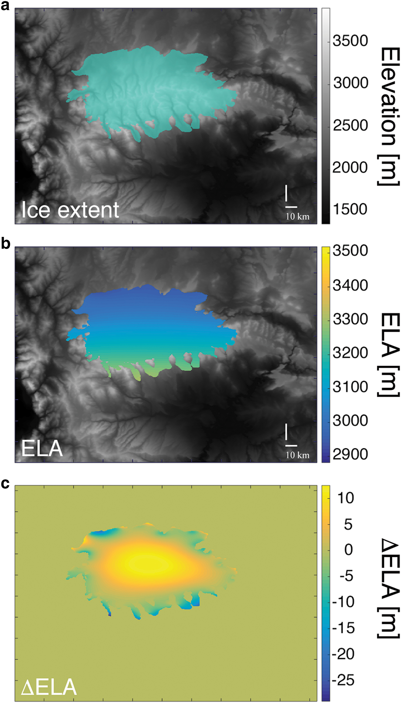
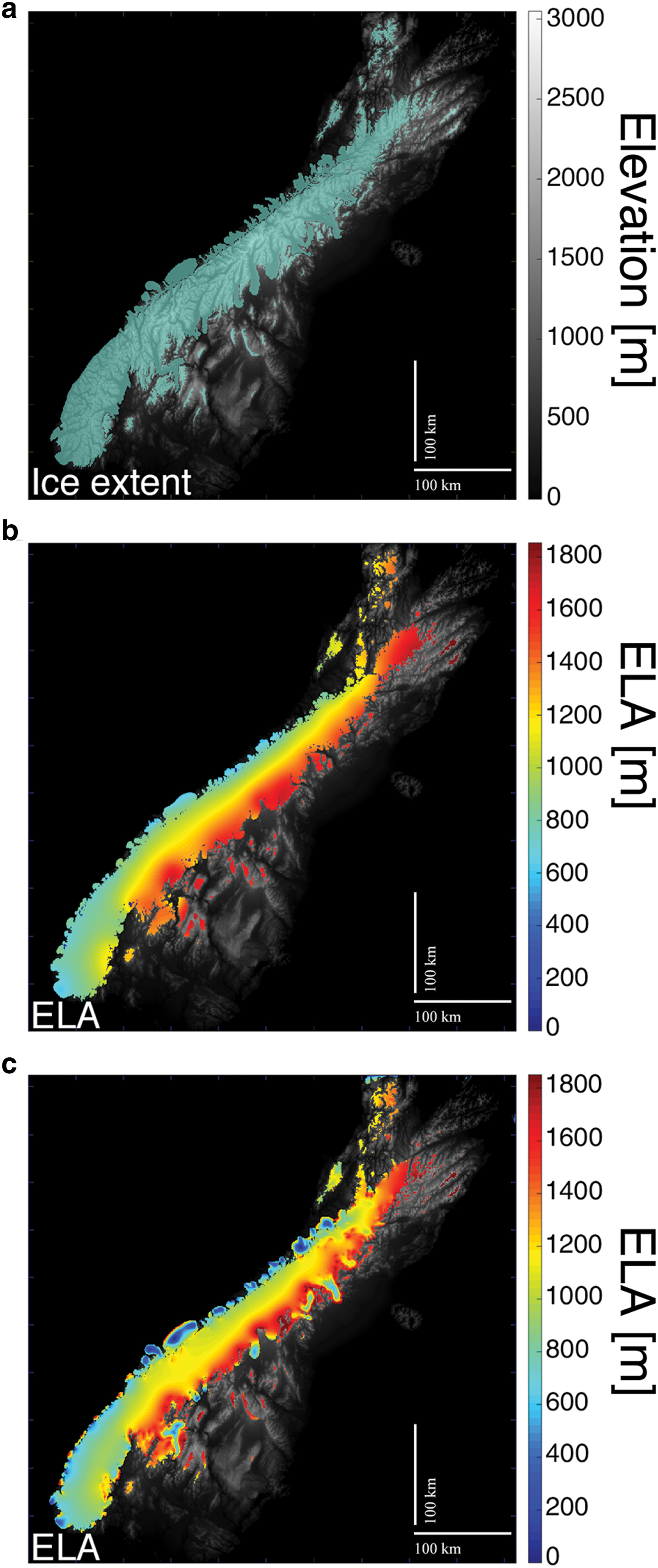
In this inversion, we constrain E(x, y) using the LGM ice extent (Barrell, Reference Barrell2011) shown in Fig. 5a. For simplicity, we use the present day bedrock with all elevations below sea level set to zero. Note, we assume that the ice extent obtained from data is reached at the same time over its entire length. All parameter values used for this test can be found in Table 5.
Application of the inverse algorithm to the South Island of New Zealand. (a) Bedrock map used (gray) with the LGM ice extent obtained from Barrell (Reference Barrell2011) (green), (b) calculated (modeled) E field using our inverse algorithm where there is ice (Test A), (c) E field calculated with the second set of parameters using our inverse algorithm where there is ice (Test B).
New Zealand inversion experiment parameters
We present two model results, test A and test B, for two different sets of τ 1, τ 2 and n sm. Both test results (Fig. 5) exhibit a clear north–south gradient in the elevation of E, as well as the west–east gradient. The N–S change could be the result of the temperature change because of the latitudinal differences, making the southern areas colder and with larger accumulation zones, and in turn lower E values. The W–E gradient reflects the influence of the westerly winds bringing precipitation to the west side, thus increasing the accumulation and lowering the altitude of E, while the east side is drier with less accumulation and higher E.
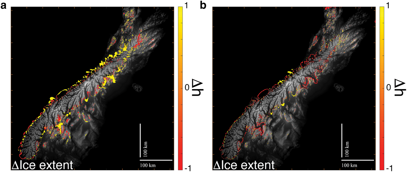
In the second test, test B, we reduce the values of the update parameters, τ 1 and τ 2, and the number of diffusion steps n sm. Reducing n sm leads to more local variations. Smaller τ 2 (five times smaller than the first test) reduces the influence of smoothing, while a smaller τ 1 results in smaller changes in E between iterations, all resulting in a more precise fit. Figs 6a and 6b show the differences between the observed (data) and calculated ice extent (model) for each test. Test B enables to better fit the data, although it does it at the expense of creating local depressions in E. This information is lost in the first test because higher smoothing, n sm, acts as a filter of local variations. It is worth keeping in mind that we are showing the results of the inversion algorithm varying only one parameter, E. This results in overfitting the data and neglecting the influence of other physical processes ignored in the model as well as approximations made in the forward model, as stated above.
Differences between the observed and modeled ice extents. (a) Test A. (b) Test B. Yellow represents areas where the data have ice but the model output does not, the red is where the model output calculates ice and the data show there was no ice in those areas.
5. DISCUSSION AND CONCLUSIONS
The main goal of this paper is to present a simple inversion method to reconstruct the spatially variable mass balance and equilibrium line altitude (E) fields using ice extent data. This approach offers the possibility of constraining past climates in glaciated mountain ranges. The inverse method is based on a Tikhonov regularization and computationally, besides the forward model, only requires the calculation of a diffusion equation. In order to show the range of applications of the method, we have constructed six experiments, both synthetic and natural, whose results are presented. To significantly reduce the calculation time necessary for our inverse model, we have implemented the codes to run on GPUs.
In the first experiment, the 2-D synthetic case, we have shown the method is capable of reconstructing a spatially variable E as well as a spatially variable β on a simple topography, consisting of a combination of two Gaussian bumps, using ice extent (Fig. 1). The second experiment is the 2-D synthetic case using real topography (Uinta Mountains) where we show that the method can successfully reconstruct spatially variable E, defined as an arctangent function from N–S, using only ice extent as constraint for our inversion. We first ran our forward ice-flow model with a chosen setup and then used the calculated ice extent as synthetic observations to invert E we originally used. The error while recovering E is less than 5% (Fig. 2c). The same was done in the experiment using ice thickness points presented in Appendix B. The difference is that instead of the ice extent we are using randomly chosen ice thickness points (Fig. 9a). Fig. 9 in Appendix B shows that the method can do the inversion successfully. When analyzing errors of the results obtained using ice extent (Fig. 2c) and ice thickness (Fig. 9c), we can see that using the ice extent the largest error is in the middle of the ice extent and the opposite effect using ice thickness. This happens because the method is more precise in places where it is better constrained by data. In the ice extent case, the errors are smaller on the edges, and in the ice thickness case, errors are larger on the edges and smaller inside the ice because of the distribution of our ice thickness points.
The influence of different number of diffusion iteration has been presented (Figs 3a, 3b). It is clear that too many diffusion iterations will result in losing the spatial variability of the result, while too little iterations will not propagate the update from the edges of the ice efficiently to its middle.
In order to verify the method, we applied it to a real case, the LGM ice extent of the South Island of New Zealand (Barrell, Reference Barrell2011). The assumption made in this experiment is that the entire ice extent is reached at the same time, representing something close to the LGM steady state. Our inversion result for the first test is similar in both pattern and values to the reconstruction done by other authors (Golledge and others, Reference Golledge2012). Fig. 5b shows a clear N–S gradient, which corresponds to the latitudinal change and is thus controlled by temperature, and a clear W–E gradient, which corresponds to the influence of the Westerlies and is thus controlled by precipitation. The second result is an example of overfitting the data. It is important to emphasize that the model setup for this experiment is simplified, which is one of the reasons for the mismatches between the observed and calculated ice extent (Fig. 6b). The bedrock topography used was the current one and the values below sea level were set to 0, thus ignoring calving. Basal sliding was parameterized as a constant value, while basal melting was not taken into account. The influence of isostasy was ignored, which is not a valid assumption for such an ice mass, and is most likely the reason E elevations are higher than expected. Despite these limitations, our method is still able to invert the spatial pattern, both the N–S and W–E gradients, and recover values close to other reconstructions.
The experiments presented show several possible applications. In order to obtain a more accurate reconstruction of mass-balance parameters for large mountain ranges, the forward model needs to be improved to include the effects of isostasy. The choice of bedrock topography for a certain time period remains a setback. The use of present day topography for LGM neglects the change in the amount, distribution and thickness of eroded and deposited sediments since the LGM. Sediment-filled valleys today might have been empty or not even eroded. This influences where our ice can flow in forward model calculations, changing the resulting ice extent and therefore our inverse calculations.
The role of β has not been fully addressed in cases where we attempt to recover E. In the presented experiments the balance gradient β was set to be constant value, and chosen arbitrarily. Future work will include an expansion of the method in order to recover both spatially variable E and β fields. Computationally, adding the inversion of another parameter in the algorithm would only require the calculation of an additional diffusion equation for β.
Similar methods to quantify climate parameters (temperature, precipitation, mass balance, equilibrium line altitude) using ice extents have been developed by other authors (Plummer and Phillips, Reference Plummer and Phillips2003; Kessler and others, Reference Kessler, Anderson and Stock2006; Golledge and others, Reference Golledge2012; Rowan and others, Reference Rowan, Brocklehurst, Schultz, Plummer, Anderson and Glasser2014). The approaches differ in defining the climate forcing (energy balance model, positive degree-day model, net mass balance Eqn (3)), and the ice-flow models used vary in complexity. Some authors use current day conditions or present-day mean annual temperature and precipitation measurements to produce scenarios where these parameters are uniformly changed, temperature reduction by −1°C or precipitation lowered by 25%, and then compare ice-flow model calculations with observations. The main difference with our approach is that our inversion algorithm works as a spatially variable optimization.
Overall, we show that by calculating only an additional diffusion equation, the method is capable to reproduce the general pattern of a spatially variable E over a mountain range using ice extent data.
ACKNOWLEDGMENTS
VV was funded through SNF grant CRSII $\_$2154434. We thank N. Golledge for providing us with the presented ice extent data. We also thank G. Prasicek and A. Licul for feedback on the text and discussion. We thank Guillaume Jouvet and an anonymous reviewer, for their constructive reviews. Matlab codes will be provided on github (https://github.com/vjeranv/IceExtentJOG.git).
APPENDIX A. NUMERICAL IMPLEMENTATION OF THE FORWARD MODEL
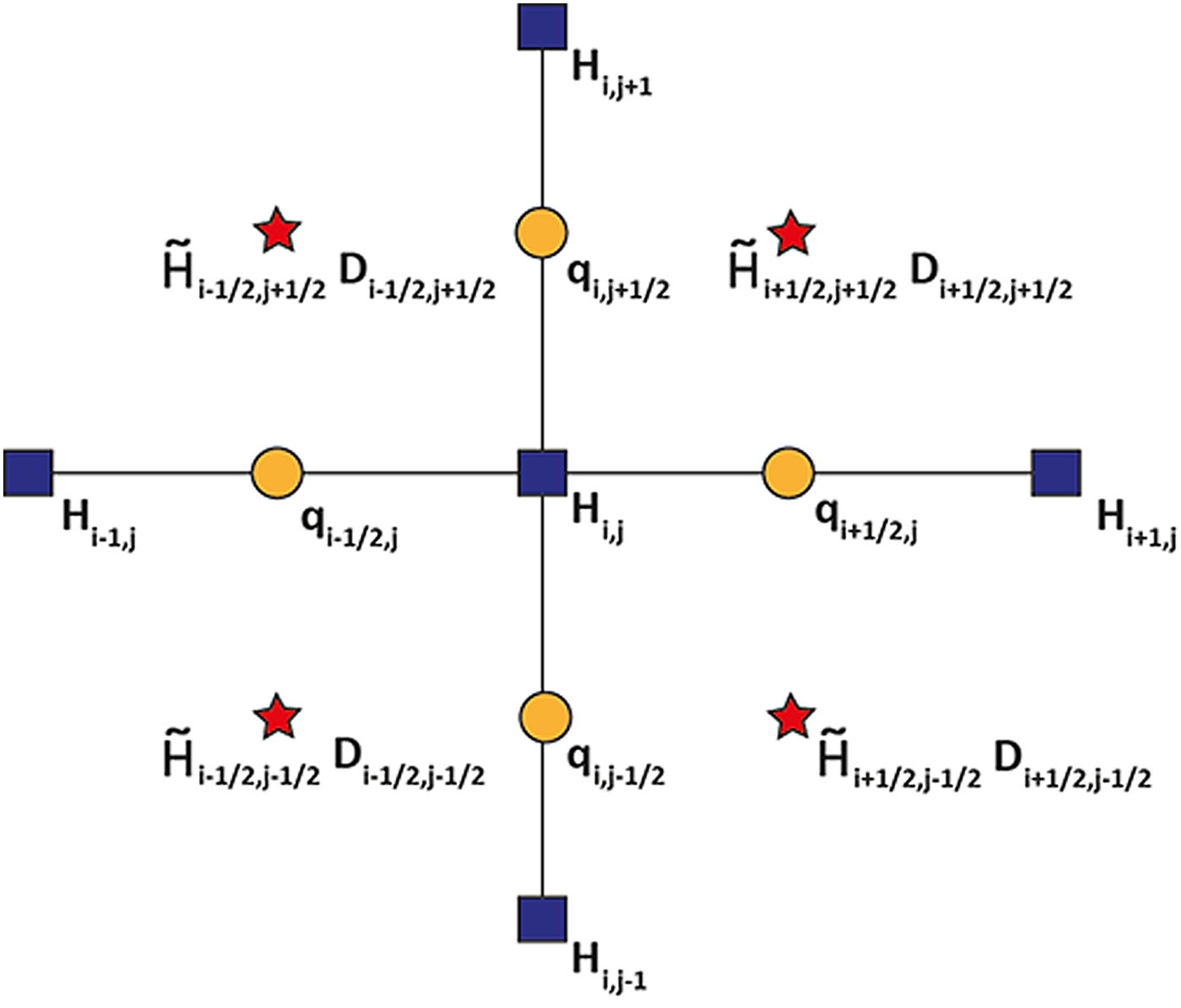
Equation (1) is solved explicitly using the finite difference method (FDM) on a staggered grid (Hindmarsh and Payne, Reference Hindmarsh and Payne1996). Figure 7 is a schematic presentation of a staggered grid. The ice thickness points are in the nodes of the grid, while fluxes are in between the nodes and the diffusivities are in the middle of the cell. To conserve mass and avoid unrealistically large fluxes that can occur when using the SIA on high resolutions and steep terrains (Plummer and Phillips, Reference Plummer and Phillips2003; Jarosch and others, Reference Jarosch, Schoof and Anslow2013), we have implemented a flux correction for diffusivity calculations based on an algorithm inspired by Wang and others (Reference Wang, Liang, Kesserwani and Hall2011). This changes how B, H and the slope  $\nabla {S}$ in Eqns (4) and (5) are calculated compared with Hindmarsh and Payne (Reference Hindmarsh and Payne1996) and substantially helps the convergence of our forward model. The topography and ice thickness are computed as follows:
 $$\tilde{B}_{i + {1 \over 2},j + {1 \over 2}} = \max [B_{i,j},B_{i + 1,j},B_{i,j + 1},B_{i + 1,j + 1}],$$
 $$\eqalign{\tilde{H}_{i + {1 \over 2},j + {1 \over 2}} &= \displaystyle{1 \over 4}\max [0,S_{i,j}-\tilde{B},S_{i + 1,j}-\tilde{B},S_{i,j + 1}\cr& \quad -\tilde{B},S_{i + 1,j + 1}-\tilde{B}],$$
Scheme representation of the staggered grid.
and the slope:
 $$\displaystyle{{\partial S} \over {\partial x}}\approx \displaystyle{\matrix{\max (\tilde{B},S_{i + 1,j})-\max (\tilde{B},S_{i,j}) + \max (\tilde{B},S_{i + 1,j + 1})-\max (\tilde{B},S_{i,j + 1})} \over {2{\rm d}x}},$$
 $$\displaystyle{{\partial S} \over {\partial y}}\approx \displaystyle{\matrix{\max (\tilde{B},S_{i,j + 1})-\max (\tilde{B},S_{i,j}) + \max (\tilde{B},S_{i + 1,j + 1})-\max (\tilde{B},S_{i + 1,j})} \over {2{\rm d}y}},$$
and the squared norm:
 $$\left\vert {\nabla S} \right\vert^2 = \bigg (\displaystyle{{\partial S} \over {\partial x}}\bigg )^2 + \bigg (\displaystyle{{\partial S} \over {\partial y}}\bigg )^2.$$
Finally, the fluxes in x and y directions are defined as:
 $$\eqalign{q_{x(i + {1 \over 2},j)} &= \displaystyle{{D_{i + {1 \over 2},j + {1 \over 2}} + D_{i + {1 \over 2},j- {1 \over 2}}} \over 2} \;\displaystyle{\matrix{\max (\max (B_{i + 1,j + 1},B_{i,j + 1}),S_{i + 1,j + 1}) -\max (\max (B_{i + 1,j + 1},B_{i,j + 1}),S_{i,j + 1})} \over {{\rm d}x}},$$
 $$\eqalign{q_{y(i,j + {1 \over 2})} &= \displaystyle{{D_{i + {1 \over 2},j + {1 \over 2}} + D_{i-{1 \over 2},j + {1 \over 2}}} \over 2} \displaystyle{\matrix{\max (\max (B_{i + 1,j + 1},B_{i + 1,j}),S_{i + 1,j + 1}) -\max (\max (B_{i + 1,j + 1},B_{i + 1,j}),S_{i + 1,j})} \over {{\rm d}y}}.$$
Combining the above expressions gives us the divergence of the flux:
 $$\nabla \cdot q\approx \displaystyle{{q_{x(i + {1 \over 2},j)}-q_{x(i-{1 \over 2},j)}} \over {{\rm d}x}} + \displaystyle{{q_{y(i,j + {1 \over 2})}-q_{y(i,j-{1 \over 2})}} \over {{\rm d}y}}.$$
Because we are solving our equations explicitly, our time step dt is strongly restricted by the Courant–Friedrichs–Lewy (CFL) condition, resulting in many forward model iterations before converging to a solution. We balance this by writing our codes for GPUs, which significantly increase our computational efficiency. GPUs are specialized for intensive highly parallel computation (graphics rendering) with more transistors devoted to data processing rather than data caching and flow control (NVIDIA, Reference NVIDIA2017). Since we are only interested in steady-state solutions of Eqn (1), we accelerate the convergence using a local time step, such that
 $${\rm d}t_{i,j}^{\rm t} = \min \left( {\displaystyle{1 \over c},c_{{\rm stab}}\displaystyle{{\min ({\rm d}x^2,{\rm d}y^2)} \over {{\rm \epsilon } + \tilde{D}_{i,j}^{\rm t} }}} \right),$$
where dx and dy is the spatial step,  ${{\rm d}t}_{i,j}^{{\rm t}}$ is the local time at each iteration, c is the maximum ice accumulation rate from Eqn (3), c stab is the time-step coefficient (Courrant number, for 2-D cases in this paper set to 1/8.1), ε is a small number (10−3) and ${\tilde {D}}_{i,j}^{\rm t}$ is the spatially averaged value of diffusivity for a given point (i, j) for the current (t) iteration. Note here that one can solve the steady-state state solution of the reaction-diffusion equation directly as a non-linear elliptic equation (Jouvet and others, Reference Jouvet, Picasso, Rappaz and Blatter2008, Reference Jouvet, Rappaz, Bueler and Blatter2011; Jouvet and Bueler, Reference Jouvet and Bueler2012).
Because solving our inverse problem explicitly may require a large number of iterations, thousands of inverse model iterations and tens to hundreds of thousands forward model iterations, or if we are interested in either high-resolution or continental scale problems, we accelerate the code on GPUs using the parallel computing platform CUDA created by NVIDIA (Micikevicius, Reference Micikevicius2009; NVIDIA, Reference NVIDIA2017). Other authors have also implemented ice-flow models for GPUs (Brædstrup and others, Reference Brædstrup, Damsgaard and Egholm2014).
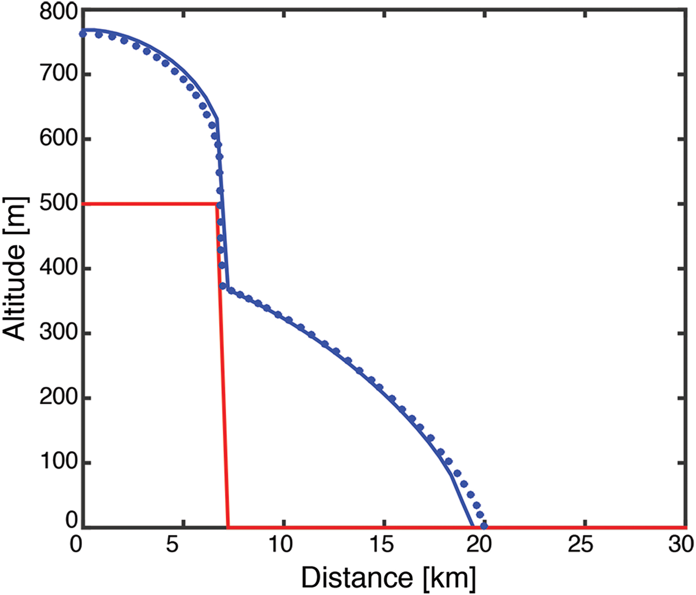
When implemented on GPU, the computation time for our forward model to calculate 110k iterations, and reach steady state, on a 1024 × 1024 grid takes around 113 s using GeForce GTX TITAN black card, and 76 s using TITAN X card, both cards were used to for our experiments and both are gaming cards, while one inverse model iteration step takes around 121 s and under 80 s, respectively. This number varies with the model of the GPU used. Just as an example to solve the same forward problem with the same setup on a professional GPU NVIDIA Tesla V100 takes 24 s. The forward model was benchmarked using the experiment proposed by Jarosch and others (Reference Jarosch, Schoof and Anslow2013) (Fig. 8).
Comparison between our numerical solution and the benchmark provided from Jarosch and others (2013). The red line represents the bedrock topography; the blue line is the analytical solution. The blue dots are the numerical solution of our forward model.
APPENDIX B. UINTA EXAMPLE USING ICE THICKNESS
Here we present the result and the values used for the inversion experiment using ice thickness values instead of ice extent. Fig. 9a represents the result of the method, while Fig. 9b shows the differences between the calculated E and a synthetic one. Parameter values used in the setup can be found in Table 6.
Results of the inversion algorithm using ice thickness points instead of ice extent (a) position of the randomly chosen ice thickness points with color corresponding to their altitude (point size not to scale), (b) is the calculated (modeled) E using our inversion algorithm, (c) difference between synthetic and calculated E where there is ice (within the moraines extent).
Uinta Mountains ice thickness experiment


 Open access